Machine Learning Summary 2017

Pieter Schaap (2014), updated by Andrew Gold (2017)

March 13, 2018

Contents

1 Lecture 1: Version Spaces 51.1 Classification Task . . . . . . . . . . . . . . . . . . . . . . . . . . . . . . . . . . . . . . . . . . . . . . . 51.2 Learning Classifiers . . . . . . . . . . . . . . . . . . . . . . . . . . . . . . . . . . . . . . . . . . . . . . . 51.3 Conjunction of Discrete Attributes . . . . . . . . . . . . . . . . . . . . . . . . . . . . . . . . . . . . . . 61.4 Find s algorithm . . . . . . . . . . . . . . . . . . . . . . . . . . . . . . . . . . . . . . . . . . . . . . . . 61.5 Version Spaces . . . . . . . . . . . . . . . . . . . . . . . . . . . . . . . . . . . . . . . . . . . . . . . . . 61.6 List elimination Algorithm . . . . . . . . . . . . . . . . . . . . . . . . . . . . . . . . . . . . . . . . . . . 61.7 Boundary Sets . . . . . . . . . . . . . . . . . . . . . . . . . . . . . . . . . . . . . . . . . . . . . . . . . 61.8 Candidate Elimination Algorithm . . . . . . . . . . . . . . . . . . . . . . . . . . . . . . . . . . . . . . . 6

1.8.1 Picking training instances . . . . . . . . . . . . . . . . . . . . . . . . . . . . . . . . . . . . . . . 71.8.2 Unanimous-Voting rule . . . . . . . . . . . . . . . . . . . . . . . . . . . . . . . . . . . . . . . . 71.8.3 Inductive Bias . . . . . . . . . . . . . . . . . . . . . . . . . . . . . . . . . . . . . . . . . . . . . 81.8.4 Unanimous Voting . . . . . . . . . . . . . . . . . . . . . . . . . . . . . . . . . . . . . . . . . . . 81.8.5 Accuracy . . . . . . . . . . . . . . . . . . . . . . . . . . . . . . . . . . . . . . . . . . . . . . . . 8

1.9 Volume Extension Approach . . . . . . . . . . . . . . . . . . . . . . . . . . . . . . . . . . . . . . . . . . 81.9.1 In Practice . . . . . . . . . . . . . . . . . . . . . . . . . . . . . . . . . . . . . . . . . . . . . . . 8

1.10 K-Version Spaces . . . . . . . . . . . . . . . . . . . . . . . . . . . . . . . . . . . . . . . . . . . . . . . . 8

2 Lecture 2: Decision Trees 92.1 Decision Trees for Classification . . . . . . . . . . . . . . . . . . . . . . . . . . . . . . . . . . . . . . . . 9

2.1.1 Now when can we use decision trees? . . . . . . . . . . . . . . . . . . . . . . . . . . . . . . . . . 92.1.2 Decision Tree Learning . . . . . . . . . . . . . . . . . . . . . . . . . . . . . . . . . . . . . . . . . 92.1.3 Entropy . . . . . . . . . . . . . . . . . . . . . . . . . . . . . . . . . . . . . . . . . . . . . . . . . 102.1.4 Information Gain . . . . . . . . . . . . . . . . . . . . . . . . . . . . . . . . . . . . . . . . . . . . 10

2.2 ID3 Algorithm . . . . . . . . . . . . . . . . . . . . . . . . . . . . . . . . . . . . . . . . . . . . . . . . . 102.2.1 Hypothesis Space . . . . . . . . . . . . . . . . . . . . . . . . . . . . . . . . . . . . . . . . . . . . 102.2.2 Inductive Bias in ID3 . . . . . . . . . . . . . . . . . . . . . . . . . . . . . . . . . . . . . . . . . 10

2.3 Overfitting, Underfitting, and Pruning . . . . . . . . . . . . . . . . . . . . . . . . . . . . . . . . . . . . 112.3.1 Causes of Overfitting . . . . . . . . . . . . . . . . . . . . . . . . . . . . . . . . . . . . . . . . . . 112.3.2 Avoiding Overfitting . . . . . . . . . . . . . . . . . . . . . . . . . . . . . . . . . . . . . . . . . . 112.3.3 Underfitting . . . . . . . . . . . . . . . . . . . . . . . . . . . . . . . . . . . . . . . . . . . . . . . 112.3.4 Identifying Overfitness, Underfitness, and Optimality . . . . . . . . . . . . . . . . . . . . . . . . 112.3.5 Growing Set vs Validation Set . . . . . . . . . . . . . . . . . . . . . . . . . . . . . . . . . . . . 122.3.6 Reduced-Error Pruning . . . . . . . . . . . . . . . . . . . . . . . . . . . . . . . . . . . . . . . . 122.3.7 Rule Post-Pruning . . . . . . . . . . . . . . . . . . . . . . . . . . . . . . . . . . . . . . . . . . . 132.3.8 Impurity . . . . . . . . . . . . . . . . . . . . . . . . . . . . . . . . . . . . . . . . . . . . . . . . . 132.3.9 Reduction of impurity . . . . . . . . . . . . . . . . . . . . . . . . . . . . . . . . . . . . . . . . . 132.3.10 Gini Index . . . . . . . . . . . . . . . . . . . . . . . . . . . . . . . . . . . . . . . . . . . . . . . 13

2.4 Dealing with continuous attributes . . . . . . . . . . . . . . . . . . . . . . . . . . . . . . . . . . . . . . 132.5 Oblique Decision Trees . . . . . . . . . . . . . . . . . . . . . . . . . . . . . . . . . . . . . . . . . . . . . 132.6 Attributes with Many Values . . . . . . . . . . . . . . . . . . . . . . . . . . . . . . . . . . . . . . . . . 14

2.6.1 Gain Ratio . . . . . . . . . . . . . . . . . . . . . . . . . . . . . . . . . . . . . . . . . . . . . . . 142.7 Missing Attribute Values . . . . . . . . . . . . . . . . . . . . . . . . . . . . . . . . . . . . . . . . . . . . 142.8 Windowing . . . . . . . . . . . . . . . . . . . . . . . . . . . . . . . . . . . . . . . . . . . . . . . . . . . 14

1

3 Lecture 3: Evaluation of Learning Models 153.1 Motivation . . . . . . . . . . . . . . . . . . . . . . . . . . . . . . . . . . . . . . . . . . . . . . . . . . . 153.2 Evaluation of Classifiers Evaluation Performance . . . . . . . . . . . . . . . . . . . . . . . . . . . . . . 15

3.2.1 Confusion Matrix . . . . . . . . . . . . . . . . . . . . . . . . . . . . . . . . . . . . . . . . . . . . 153.2.2 Metrics . . . . . . . . . . . . . . . . . . . . . . . . . . . . . . . . . . . . . . . . . . . . . . . . . 153.2.3 Confidence Intervals for Estimates on Classification Performance . . . . . . . . . . . . . . . . . 163.2.4 Metric Evaluation TL;DR . . . . . . . . . . . . . . . . . . . . . . . . . . . . . . . . . . . . . . . 16

3.3 Comparing Data-Mining Classifier . . . . . . . . . . . . . . . . . . . . . . . . . . . . . . . . . . . . . . 163.3.1 Counting the Costs . . . . . . . . . . . . . . . . . . . . . . . . . . . . . . . . . . . . . . . . . . . 163.3.2 Cost-Sensitive Classification . . . . . . . . . . . . . . . . . . . . . . . . . . . . . . . . . . . . . . 16

3.4 Lift Charts . . . . . . . . . . . . . . . . . . . . . . . . . . . . . . . . . . . . . . . . . . . . . . . . . . . 173.4.1 Generating a Lift Chart . . . . . . . . . . . . . . . . . . . . . . . . . . . . . . . . . . . . . . . . 17

3.5 ROC Curves . . . . . . . . . . . . . . . . . . . . . . . . . . . . . . . . . . . . . . . . . . . . . . . . . . 173.5.1 ROC Convex Hull . . . . . . . . . . . . . . . . . . . . . . . . . . . . . . . . . . . . . . . . . . . 173.5.2 Iso-Accuracy Lines . . . . . . . . . . . . . . . . . . . . . . . . . . . . . . . . . . . . . . . . . . . 173.5.3 Contructing ROC Curve for 1 Classifier . . . . . . . . . . . . . . . . . . . . . . . . . . . . . . . 173.5.4 Area Under Curve Metric (AUC) . . . . . . . . . . . . . . . . . . . . . . . . . . . . . . . . . . . 17

4 Lecture 4: Bayesian Learning 184.1 Introduction . . . . . . . . . . . . . . . . . . . . . . . . . . . . . . . . . . . . . . . . . . . . . . . . . . . 184.2 Bayes Theorem . . . . . . . . . . . . . . . . . . . . . . . . . . . . . . . . . . . . . . . . . . . . . . . . . 184.3 Maximum a Posteriori Hypothesis (MAP) . . . . . . . . . . . . . . . . . . . . . . . . . . . . . . . . . . 184.4 Useful Formulas . . . . . . . . . . . . . . . . . . . . . . . . . . . . . . . . . . . . . . . . . . . . . . . . . 184.5 Brute Force MAP hypothesis learner . . . . . . . . . . . . . . . . . . . . . . . . . . . . . . . . . . . . . 184.6 Minimum Description Length Principle . . . . . . . . . . . . . . . . . . . . . . . . . . . . . . . . . . . . 184.7 Bayes Optimal Classifier . . . . . . . . . . . . . . . . . . . . . . . . . . . . . . . . . . . . . . . . . . . . 194.8 Gibbs Classifier . . . . . . . . . . . . . . . . . . . . . . . . . . . . . . . . . . . . . . . . . . . . . . . . . 194.9 Naıve Bayes Classifier . . . . . . . . . . . . . . . . . . . . . . . . . . . . . . . . . . . . . . . . . . . . . 19

5 Lecture 5: Linear Regression 205.1 Supervised Learning: Regression . . . . . . . . . . . . . . . . . . . . . . . . . . . . . . . . . . . . . . . 20

5.1.1 Regression versus Classification . . . . . . . . . . . . . . . . . . . . . . . . . . . . . . . . . . . . 205.2 Linear Regression . . . . . . . . . . . . . . . . . . . . . . . . . . . . . . . . . . . . . . . . . . . . . . . . 205.3 Cost function intuition . . . . . . . . . . . . . . . . . . . . . . . . . . . . . . . . . . . . . . . . . . . . . 20

5.3.1 Least Squares Error . . . . . . . . . . . . . . . . . . . . . . . . . . . . . . . . . . . . . . . . . . 225.4 Gradient descent . . . . . . . . . . . . . . . . . . . . . . . . . . . . . . . . . . . . . . . . . . . . . . . . 22

5.4.1 Choosing Learning Rate . . . . . . . . . . . . . . . . . . . . . . . . . . . . . . . . . . . . . . . . 225.4.2 Multiple Features . . . . . . . . . . . . . . . . . . . . . . . . . . . . . . . . . . . . . . . . . . . . 22

5.5 Normal Equation . . . . . . . . . . . . . . . . . . . . . . . . . . . . . . . . . . . . . . . . . . . . . . . . 235.5.1 Feature Scaling . . . . . . . . . . . . . . . . . . . . . . . . . . . . . . . . . . . . . . . . . . . . . 235.5.2 The Algorithm . . . . . . . . . . . . . . . . . . . . . . . . . . . . . . . . . . . . . . . . . . . . . 23

5.6 Normal Equation vs Gradient Descent . . . . . . . . . . . . . . . . . . . . . . . . . . . . . . . . . . . . 235.7 Finding the ”right” model . . . . . . . . . . . . . . . . . . . . . . . . . . . . . . . . . . . . . . . . . . . 23

5.7.1 Regularization . . . . . . . . . . . . . . . . . . . . . . . . . . . . . . . . . . . . . . . . . . . . . 23

6 Lecture 6: Logistic Regression and Artificial Neural Networks 256.1 Logistic Regression . . . . . . . . . . . . . . . . . . . . . . . . . . . . . . . . . . . . . . . . . . . . . . . 25

6.1.1 Sigmoid Logistic Regression . . . . . . . . . . . . . . . . . . . . . . . . . . . . . . . . . . . . . . 256.1.2 Non-Linear Decision Boundaries . . . . . . . . . . . . . . . . . . . . . . . . . . . . . . . . . . . 25

6.2 Cost Function . . . . . . . . . . . . . . . . . . . . . . . . . . . . . . . . . . . . . . . . . . . . . . . . . . 256.3 Gradient Descent for Logistic Regression . . . . . . . . . . . . . . . . . . . . . . . . . . . . . . . . . . . 266.4 Multi-Class Problems . . . . . . . . . . . . . . . . . . . . . . . . . . . . . . . . . . . . . . . . . . . . . 266.5 Artificial Neural Networks . . . . . . . . . . . . . . . . . . . . . . . . . . . . . . . . . . . . . . . . . . . 26

6.5.1 Forward Propagation . . . . . . . . . . . . . . . . . . . . . . . . . . . . . . . . . . . . . . . . . . 266.5.2 Learning The Weights . . . . . . . . . . . . . . . . . . . . . . . . . . . . . . . . . . . . . . . . . 276.5.3 Properties Of Neural Networks . . . . . . . . . . . . . . . . . . . . . . . . . . . . . . . . . . . . 27

2

7 Lecture 7: Recommender Systems 287.1 Collaborative Filtering . . . . . . . . . . . . . . . . . . . . . . . . . . . . . . . . . . . . . . . . . . . . . 287.2 Content Based Approach . . . . . . . . . . . . . . . . . . . . . . . . . . . . . . . . . . . . . . . . . . . 287.3 Collaborative Filtering . . . . . . . . . . . . . . . . . . . . . . . . . . . . . . . . . . . . . . . . . . . . . 28

7.3.1 Collaborative Filtering Algorithm . . . . . . . . . . . . . . . . . . . . . . . . . . . . . . . . . . . 297.3.2 Mean Normalization . . . . . . . . . . . . . . . . . . . . . . . . . . . . . . . . . . . . . . . . . . 29

7.4 Support Vector Machines . . . . . . . . . . . . . . . . . . . . . . . . . . . . . . . . . . . . . . . . . . . 297.4.1 Linear SVMs . . . . . . . . . . . . . . . . . . . . . . . . . . . . . . . . . . . . . . . . . . . . . . 297.4.2 Non-Linear SVMs . . . . . . . . . . . . . . . . . . . . . . . . . . . . . . . . . . . . . . . . . . . 297.4.3 Logistic Regression to SVM . . . . . . . . . . . . . . . . . . . . . . . . . . . . . . . . . . . . . . 297.4.4 Kernels . . . . . . . . . . . . . . . . . . . . . . . . . . . . . . . . . . . . . . . . . . . . . . . . . 297.4.5 Cost Function . . . . . . . . . . . . . . . . . . . . . . . . . . . . . . . . . . . . . . . . . . . . . . 30

7.5 Compare SVM . . . . . . . . . . . . . . . . . . . . . . . . . . . . . . . . . . . . . . . . . . . . . . . . . 30

8 Lecture 8: 318.1 Nearest Neighbor Algorithm . . . . . . . . . . . . . . . . . . . . . . . . . . . . . . . . . . . . . . . . . . 31

8.1.1 Properties . . . . . . . . . . . . . . . . . . . . . . . . . . . . . . . . . . . . . . . . . . . . . . . . 318.1.2 Decision Boundaries . . . . . . . . . . . . . . . . . . . . . . . . . . . . . . . . . . . . . . . . . . 318.1.3 Lazy vs Eager Learning . . . . . . . . . . . . . . . . . . . . . . . . . . . . . . . . . . . . . . . . 318.1.4 Inductive vs Transductive learning . . . . . . . . . . . . . . . . . . . . . . . . . . . . . . . . . . 318.1.5 Semi-Supervised Learning . . . . . . . . . . . . . . . . . . . . . . . . . . . . . . . . . . . . . . . 318.1.6 Distance Definition . . . . . . . . . . . . . . . . . . . . . . . . . . . . . . . . . . . . . . . . . . . 328.1.7 Normalization of Attributes . . . . . . . . . . . . . . . . . . . . . . . . . . . . . . . . . . . . . . 328.1.8 Weighted Distances . . . . . . . . . . . . . . . . . . . . . . . . . . . . . . . . . . . . . . . . . . 328.1.9 More distances . . . . . . . . . . . . . . . . . . . . . . . . . . . . . . . . . . . . . . . . . . . . . 32

8.2 Distance-weighted kNN . . . . . . . . . . . . . . . . . . . . . . . . . . . . . . . . . . . . . . . . . . . . 338.2.1 Edited k-nearest neighbor . . . . . . . . . . . . . . . . . . . . . . . . . . . . . . . . . . . . . . . 33

8.3 Pipeline Filters . . . . . . . . . . . . . . . . . . . . . . . . . . . . . . . . . . . . . . . . . . . . . . . . . 338.4 kD-trees . . . . . . . . . . . . . . . . . . . . . . . . . . . . . . . . . . . . . . . . . . . . . . . . . . . . . 338.5 Local Learning . . . . . . . . . . . . . . . . . . . . . . . . . . . . . . . . . . . . . . . . . . . . . . . . . 348.6 Comments on k-NN . . . . . . . . . . . . . . . . . . . . . . . . . . . . . . . . . . . . . . . . . . . . . . 348.7 Decision Boundaries . . . . . . . . . . . . . . . . . . . . . . . . . . . . . . . . . . . . . . . . . . . . . . 348.8 Sequential Covering Approaches . . . . . . . . . . . . . . . . . . . . . . . . . . . . . . . . . . . . . . . 34

8.8.1 Candidate Literals . . . . . . . . . . . . . . . . . . . . . . . . . . . . . . . . . . . . . . . . . . . 358.8.2 Sequential covering . . . . . . . . . . . . . . . . . . . . . . . . . . . . . . . . . . . . . . . . . . . 358.8.3 Heuristics . . . . . . . . . . . . . . . . . . . . . . . . . . . . . . . . . . . . . . . . . . . . . . . . 36

8.9 Example-driven Top-down Rule induction . . . . . . . . . . . . . . . . . . . . . . . . . . . . . . . . . . 368.10 Avoiding over-fitting . . . . . . . . . . . . . . . . . . . . . . . . . . . . . . . . . . . . . . . . . . . . . . 36

9 Lecture 9: Clustering 379.1 Unsupervised Learning . . . . . . . . . . . . . . . . . . . . . . . . . . . . . . . . . . . . . . . . . . . . . 379.2 Clustering . . . . . . . . . . . . . . . . . . . . . . . . . . . . . . . . . . . . . . . . . . . . . . . . . . . . 379.3 Similarity Measures . . . . . . . . . . . . . . . . . . . . . . . . . . . . . . . . . . . . . . . . . . . . . . 379.4 Flat vs. Hierarchical Clustering . . . . . . . . . . . . . . . . . . . . . . . . . . . . . . . . . . . . . . . . 379.5 Extensional vs Intensional Clustering . . . . . . . . . . . . . . . . . . . . . . . . . . . . . . . . . . . . . 379.6 Cluster Assignment . . . . . . . . . . . . . . . . . . . . . . . . . . . . . . . . . . . . . . . . . . . . . . . 389.7 Major Clustering Approaches . . . . . . . . . . . . . . . . . . . . . . . . . . . . . . . . . . . . . . . . . 389.8 Hierarchical Clustering . . . . . . . . . . . . . . . . . . . . . . . . . . . . . . . . . . . . . . . . . . . . . 38

9.8.1 Dendogram . . . . . . . . . . . . . . . . . . . . . . . . . . . . . . . . . . . . . . . . . . . . . . . 389.8.2 Bottom up Hierarchical Clustering . . . . . . . . . . . . . . . . . . . . . . . . . . . . . . . . . . 38

9.9 Distance between two clusters . . . . . . . . . . . . . . . . . . . . . . . . . . . . . . . . . . . . . . . . . 38

3

10 Lecture 10: 3910.1 Reinforcement learning . . . . . . . . . . . . . . . . . . . . . . . . . . . . . . . . . . . . . . . . . . . . . 3910.2 Optimal Policy . . . . . . . . . . . . . . . . . . . . . . . . . . . . . . . . . . . . . . . . . . . . . . . . . 3910.3 Q-learning Algorithm . . . . . . . . . . . . . . . . . . . . . . . . . . . . . . . . . . . . . . . . . . . . . 39

10.3.1 Q-Learning Intuition . . . . . . . . . . . . . . . . . . . . . . . . . . . . . . . . . . . . . . . . . . 3910.3.2 Learning the Q-Values . . . . . . . . . . . . . . . . . . . . . . . . . . . . . . . . . . . . . . . . . 4010.3.3 Q-Learning Optimality . . . . . . . . . . . . . . . . . . . . . . . . . . . . . . . . . . . . . . . . . 4010.3.4 Accelerating the Q-Learning Process . . . . . . . . . . . . . . . . . . . . . . . . . . . . . . . . . 4010.3.5 Q-Learning Summary . . . . . . . . . . . . . . . . . . . . . . . . . . . . . . . . . . . . . . . . . 40

10.4 Online Learning and SARSA . . . . . . . . . . . . . . . . . . . . . . . . . . . . . . . . . . . . . . . . . 4010.5 Expectation Maximization . . . . . . . . . . . . . . . . . . . . . . . . . . . . . . . . . . . . . . . . . . . 41

4

1 Lecture 1: Version Spaces

Version space learning is a logical approach to machine learning, specifically binary classification. Version spacelearning algorithms search a predefined space of hypotheses, viewed as a set of logical sentences. Formally, thehypothesis space is a disjunction:

• H1 ∨H2 ∨ ... ∨Hn

(i.e., either hypothesis 1 is true, or hypothesis 2, or any subset of the hypotheses 1 through n). A version spacelearning algorithm is presented with examples, which it will use to restrict its hypothesis space; for each example x,the hypotheses that are inconsistent with x are removed from the space. This iterative refining of the hypothesis spaceis called the candidate elimination algorithm (see 1.8), the hypothesis space maintained inside the algorithm itsversion space.

Overview

• Classification Task

• FindS algorithm

• Version Spaces

• List Elimination Algorithm

• Boundary Sets and Candidate Elimination Algorithm

• Properties of Version Spaces

• Inductive Bias

• Version Spaces and Consistency Tests

• Volume Extension and k-Version Spaces

1.1 Classification Task

• Class is a set of objects with the same appearance structure or function.

• Elements are aspects of one (or more) objects.

• Classifiers are a set of elements that indicate that an object belongs to a certain class.

• The hypothesis space used by a machine learning system is the set of all hypotheses that might possibly bereturned by it (as being true).

So a classification task consists out of 4 properties: X, Y, H and D where: X:= The version space Y:= The evaluationof an object in the version space (done by H) H:= The hypothesis space D:= The training data

Binary Classification task; e.g. |Y | = 2 Multi-Class Classification task; e.g. |Y | >= 2

1.2 Learning Classifiers

Essentially a search in the hypothesis space where the goal is to find a hypothesis to best fit the training data D. If thishypothesis is consistent with a sufficiently large set of training data it will give a good approximation of other unob-served instances. Consistency Criterion: Hypothesis h is consistent with D ⇔ h(x) = y for each instance (x, y) in D

When ordering the hypothesis from ”General” to ”Specific” the following logic can be applied:(∀h1, h2 ∈ H)((h1 ≥ h2)⇔ (∀x ∈ X)(h1(x) = 1⇐ h1(x) = 1))

5

1.3 Conjunction of Discrete Attributes

How to generalize a hypothesis (h) with respect to an instance (x)?For every attribute Ai in the hypothesis h where Ai is specified and contradicts the instance x: Set Ai of h to ?(unspecified).

And how do we make it more specific? First we create an empty set that we call the specializations. Assumingthat the instance x is a positive object;For every attribute value v of Ai of h that is not specified (=?) we create a specialization s that is equal to h andset the value of attribute Ai of s to v. We then set the specializations set to be the union of itself and s. (end for)

1.4 Find s algorithm

initialize s to the most specific hypothesis in H.For every training instance x we check if x is positive; if so, we generalize s against x. if it is not we check if s(x) =1 (equals true) and if that is the case we stop.

1.5 Version Spaces

Definition: The version space VS(D) for the training data D is the set of all the consistent hypotheses in H. or inmathematical notation:V S(D) = {h ∈ H|consistent(h,D)}

The classification rule of a version space is the unanimous voting rule i.e. every hypothesis must evaluate objectx as true in order to be classified.

1.6 List elimination Algorithm

More commonly known as the ”List-then-eliminate algorithm”. Basically takes a list of all the Hypotheses in H andfor every training instance it removes every hypothesis from the list that is not consistent with the training instance.

1.7 Boundary Sets

Two types:

• Minimal Boundary Set (Most specific Set)

• Maximal Boundary Set (Most General Set)

In essence this means that if an hypothesis space H is admissible (fits) the training data D, then there exists anhypothesis s in the minimal boundary set and an hypothesis g in the maximal boundary set such that for everyhypothesis in H the following holds: s ≤ h ≤ g

or more formally: (∀h ∈ H)((h ∈ V S(D)) ⇐⇒ (∃s ∈ S(D))(∃g ∈ G(D))(s ≤ h ≤ g)).

1.8 Candidate Elimination Algorithm

The candidate elimination algorithm incrementally builds the version space given a hypothesis space H and a set Eof examples. The examples are added one by one; each example possibly shrinks the version space by removing thehypotheses that are inconsistent with the example. The candidate elimination algorithm does this by updating thegeneral and specific boundary for each new example.

• Candidate Elimination Algorithm(X,Y,E,H)

– Inputs:

∗ X: set of input features, X=X1,...,Xn

∗ Y: target feature

∗ E: set of examples from which to learn

∗ H: hypothesis space

– Output:

∗ general boundary GH

6

∗ specific boundary SH consistent with E

– Local

∗ G: set of hypotheses in H

∗ S: set of hypotheses in H

– Let G={true}, S={false};1. for each e ∈ E do:

(a) if (e is a positive example) then compare e to Gi−1 (of the previous example).

i. Elements of G that classify e as negative are removed from G;

ii. Each element g in Gi−1 that contradicts with the same element in example e is removed fromthe new general set G for example e.

iii. Non-maximal hypotheses are removed from S;

(b) else if (e is a negative example) then compare e to S of previous example:

i. Elements of S that classify e as positive are removed from S;

ii. Each element s of Si−1 that contradicts with the same element in the negative example e goesinto a new general set G where the contradicting element is the only specific element, and allother elements are marked with a ?. If there are multiple elements e that contradict with thesame element in S, a new general set G is made. All contradictions get their own set G withonly ?’s and the single contradicting element.

∗ Each new general set is bound to the specific contradiction of the previous S.

∗ Then we eliminate from the new S (belonging to ei) the negative elements in e that alignwith the specific set S from the previous example.

iii. Non-minimal hypotheses are removed from G.

More elaborate explanation: http://artint.info/html/ArtInt_193.html

The candidate elimination algorithm converges to a correct description if:

• there are no errors in the training data.

• When the classifier of the target class is H (i have no idea what he means)

1.8.1 Picking training instances

When picking the next training instance the learner should request instances that correspond to exactly half of thedescriptions in the Version Space. Therefore the description of the target concept can be found with log2|V S| numberof instances.

1.8.2 Unanimous-Voting rule

• Definition 1: This basically means that both (upper and lower) boundaries should agree on whether a traininginstance is true or false and do not contradict the training instance. (true if the training instance is true, falseif the training instance is false).

• Definition 2: Given version space VS(D), an instance x ∈ X receives a classification VS(D)(x) defined as follows:

V S(D)(x) =

{y : V S(D) 6= ∅ ∧ (∀h ∈ V S(D))y = h(x)”?” : Otherwise.

• Definition 3: Volume V(VS(D)) of version space VS(D) is the set of all instances that are not classified byVS(D).

7

1.8.3 Inductive Bias

Completeness of a version space: Version Space = complete ↔ for any dataset D there exists a hypothesis in H s.t.H is consistent with D

Now the inductive Bias of Version Spaces is the assumption that a version space is incomplete! So when do wespeak of a correct inductive bias? Well, that is when the target hypothesis t is in the hypothesis space H and thetraining data are noise free (all fields are known and are correct). According to the internet: Inductive Bias = Theassumption that the target concept is contained in the hypothesis space (doesn’t this contradict the slides? (abovestatement))

However, upon reviewing this with someone we concluded that it is possible that the inductive bias is simplythe set of rules that we found from inductive learning over the training data which can then be used to classify newinstances. WE THINK!

1.8.4 Unanimous Voting

Theorem: For any instance x ∈ X and class y ∈ Y :(∀h ∈ V S(D))(h(x) = y) ↔ (∀y′ ∈ Y \ {y})V S(D ∪ {(x, y′)}) = ∅. In other words what this says is that for everyhypothesis in the version space that classifies instance x as class y it holds that for every other class x cannot beclassified as true. or in other other words: The Theorem states the unanimous-voting rule can be implemented if wehave an algorithm to test version spaces for collapse.

Unanimous voting can be used to determine whether we can correctly classify an instance.

1.8.5 Accuracy

So when can we reach 100% accuracy and when not? Well there are 3 cases:

• Case 1: Data is noise free and the hypothesis space H contains the target classifier. (100% accuracy)

• Case 2: The hypothesis space H does not contain the target classifier and thus we do not know for sure whichclass the instance has.

• Case 3: The training data contains noise. Therefore we cannot be certain if we are classifying correctly.

1.9 Volume Extension Approach

The volume-extension approach is a new approach to overcome the problems with noisy training data and inexpressivehypothesis spaces. If a version space V S(I+, I ) ⊆ H misclassifies instances, the approach is to find a new hypothesisspace H0 s.t. the volume of version space V S0(I+, I ) ⊆ H0 grows and blocks instance misclassifications.

Theorem: Consider hypothesis space H and H’ such that:(∀D)((∃h ∈ H) that is consistend(h,D) then: (∃h′ ∈ H ′) that is consistent(h’,D)) as well. Then, for any data set

D: V (V S(D)) ⊆ V (V S′(D))

1.9.1 In Practice

• Case 2: H does not contain the target classifier. The solution in this case is to add a classifier that classifiesthe instance differently than the classifiers in VS(D). In other words, we extend the volume of VS(D)

• Case 3: When the datasets are noisy. The solution is again to add a classifier that classifies the instancesdifferently than the classifiers in VS(D) and we extend the volume of VS(D) again.

1.10 K-Version Spaces

k-Version spaces were introduced to handle noisy data. They were defined as sets of k-consistent hypotheses; i.e.hypotheses consistent with all but k instances. Definition 1: Given a classifier space H and training data D, thek-version space V Sk(D) is:

V Sk(D) = {h ∈ H|consistenk(h,D)},whereconsistentk(h,D)↔ (∃Dk ⊆ Pk(D))(∀(x, y) ∈ Dk)(y = h(x))

Theorem: if k2 > k1 then, for any data set D:V (V Sk1(D))TODOV (V Sk2(D))

8

2 Lecture 2: Decision Trees

Overview

Decision Trees for Classification

• Definition

• Classification Problems for Decision Trees

• Entropy and Information Gain

• Learning Decision Trees

• Overfitting, Underfitting, and Pruning

• Validation Set vs Growing Set

• Handling Continuous-Valued Attributes

• Handling Missing Attribute Values

• Alternative Measures for Selecting Attributes

• Handling Large Data: Windowing

2.1 Decision Trees for Classification

Definition: A decision tree is a tree where:

• Each interior node tests an attribute of some data set

• Each branch corresponds to an attribute value

• Each leaf node is labeled with a class (class node) of the data

2.1.1 Now when can we use decision trees?

Each instance consists of an attribute with discrete values; e.g. weather forecast = sunny or weather forecast =rainy. The classification has to happen over discrete values (true or false; yes or no; 0 or 1 etc.) Decision trees canhave disjunctive descriptions; i.e. a path in a tree represents a disjunctive description. If the training set containserrors or missing data then the decision tree is robust enough to deal with this.

2.1.2 Decision Tree Learning

There is a basic algorithm for learning a decision tree:

1. A ← the ”best” decision attribute for a node N.

2. Assign A as decision attribute for the node N.

3. For each value of A, create new descendant of the node N.

4. Sort training examples to leaf nodes.

5. IF training examples perfectly classified, THEN STOP.ELSE iterate over new leaf nodes

So in short what it does is for every decision attribute (e.g. weather forecast) create a child node and ”list” allinstances that apply to the leaf node. If it is all classified correctly (no leaf node contains a true and a false at thesame time).

9

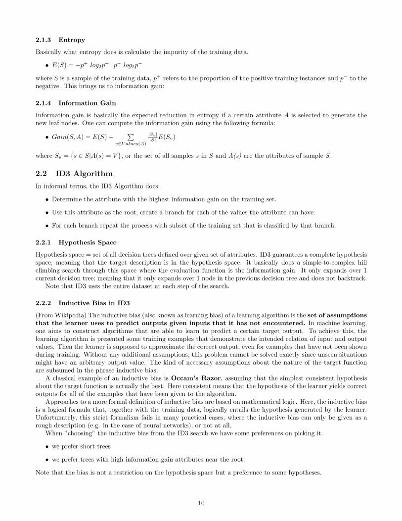
2.1.3 Entropy

Basically what entropy does is calculate the impurity of the training data.

• E(S) = −p+ log2p+ p− log2p

−

where S is a sample of the training data, p+ refers to the proportion of the positive training instances and p− to thenegative. This brings us to information gain:

2.1.4 Information Gain

Information gain is basically the expected reduction in entropy if a certain attribute A is selected to generate thenew leaf nodes. One can compute the information gain using the following formula:

• Gain(S,A) = E(S)−∑

v∈V alues(A)

|Sv||S| E(Sv)

where Sv = {s ∈ S|A(s) = V }, or the set of all samples s in S and A(s) are the attributes of sample S.

2.2 ID3 Algorithm

In informal terms, the ID3 Algorithm does:

• Determine the attribute with the highest information gain on the training set.

• Use this attribute as the root, create a branch for each of the values the attribute can have.

• For each branch repeat the process with subset of the training set that is classified by that branch.

2.2.1 Hypothesis Space

Hypothesis space = set of all decision trees defined over given set of attributes. ID3 guarantees a complete hypothesisspace; meaning that the target description is in the hypothesis space. it basically does a simple-to-complex hillclimbing search through this space where the evaluation function is the information gain. It only expands over 1current decision tree; meaning that it only expands over 1 node in the previous decision tree and does not backtrack.

Note that ID3 uses the entire dataset at each step of the search.

2.2.2 Inductive Bias in ID3

(From Wikipedia) The inductive bias (also known as learning bias) of a learning algorithm is the set of assumptionsthat the learner uses to predict outputs given inputs that it has not encountered. In machine learning,one aims to construct algorithms that are able to learn to predict a certain target output. To achieve this, thelearning algorithm is presented some training examples that demonstrate the intended relation of input and outputvalues. Then the learner is supposed to approximate the correct output, even for examples that have not been shownduring training. Without any additional assumptions, this problem cannot be solved exactly since unseen situationsmight have an arbitrary output value. The kind of necessary assumptions about the nature of the target functionare subsumed in the phrase inductive bias.

A classical example of an inductive bias is Occam’s Razor, assuming that the simplest consistent hypothesisabout the target function is actually the best. Here consistent means that the hypothesis of the learner yields correctoutputs for all of the examples that have been given to the algorithm.

Approaches to a more formal definition of inductive bias are based on mathematical logic. Here, the inductive biasis a logical formula that, together with the training data, logically entails the hypothesis generated by the learner.Unfortunately, this strict formalism fails in many practical cases, where the inductive bias can only be given as arough description (e.g. in the case of neural networks), or not at all.

When ”choosing” the inductive bias from the ID3 search we have some preferences on picking it.

• we prefer short trees

• we prefer trees with high information gain attributes near the root.

Note that the bias is not a restriction on the hypothesis space but a preference to some hypotheses.

10

2.3 Overfitting, Underfitting, and Pruning

Overfitting is the concept where a model contains more parameters than the data can reasonably suggest, or insimpler terms: your models are learning too much from noise, and interpreting noise as actually meaningful data.Therefore, overfit statistical models can suggest things that aren’t true, because it has learned too much from noise.

Overfitting generally happens when you have too many adjustable parameters than what would be optimal, ormore simply by being more complicated than necessary. Therefore, your model may ”learn” from noise a specificexample and assume that is actually an important characteristic, when in fact it was merely an outlier. Overfittingcan be avoided by being as general as possible, and then furthermore by finding some form of average between anoverfit and underfit model.

In science the principle of Occam’s Razor is the concept that the simplest solution is often the best or ”mostcorrect.” Essentially: ”Do not make things more complicated than necessary”. This view is also often used in machinelearning. When working with decision trees this holds as well. Big (complex) decision trees shelter the thread ofover-fitting. The bigger the tree, the bigger the risk of over-fitting.

2.3.1 Causes of Overfitting

(from Wikipedia) Overfitting is especially likely in cases where learning was performed too long or where trainingexamples are rare, causing the learner to adjust to very specific random features of the training data, that haveno causal relation to the target function. In this process of overfitting, the performance on the trainingexamples still increases while the performance on unseen data becomes worse.

Generally, a learning algorithm is said to overfit relative to a simpler one if it is more accurate in fitting knowndata (hindsight) but less accurate in predicting new data (foresight). One can intuitively understand overfitting fromthe fact that information from all past experience can be divided into two groups: information that is relevant for thefuture and irrelevant information (”noise”). Everything else being equal, the more difficult a criterion is to predict(i.e., the higher its uncertainty), the more noise exists in past information that needs to be ignored. The problem isdetermining which part to ignore. A learning algorithm that can reduce the chance of fitting noise is called robust.

• Noisy training data.

• Small number of instances are associated with leaf nodes. (coincidental regularities may occur that are unrelatedto target concept).

2.3.2 Avoiding Overfitting

• Pre-pruning: Stop the tree from growing before it matches the training data perfectly.

– When to stop? (difficult) Some of the solutions:

∗ Stop when the number of leaf nodes becomes less than M training instances.

∗ Use a Validation Set: a set of instances used to evaluate the utility of nodes in decision trees.Usually the training data is randomly split into a growing set and a validation set. The set must bechosen in a manner that it is unlikely to have the same errors as the growing set. For example seeReduced-Error Pruning further on in this document.

• Post-pruning: Allow the tree to over-fit, then tweak the tree afterwards. Can also couple an overfit model(s)with underfit model(s) and finding some form of average between the two.

2.3.3 Underfitting

Underfitting occurs when a statistical model or machine learning algorithm cannot adequately capture the underlyingstructure of the data. It occurs when the model or algorithm does not fit the data enough. Underfitting occurs if themodel or algorithm shows low variance but high bias (to contrast the opposite, overfitting from high variance andlow bias). It is often a result of an excessively simple model.

2.3.4 Identifying Overfitness, Underfitness, and Optimality

• Overfitness:

– When performance on training data increases while performance on unseen data/testing data decreases.The training data is being learned while the unseen data is being misclassified. On a graph it can also beidentified by a wide gap between the training data’s accuracy vs the testing data accuracy.

11

• Underfitness:

– When performance is poor (error is high, accuracy is low) on both the training AND unseen/testing data.The model is too generic, and it is not learning enough, leading to poor performance all around. Can beidentified on a graph by seeing low accuracy rates for both sets of data.

• Optimality:

– When performance on both training data and the unseen/testing data follows a very similar pattern,meaning that something that is affecting the training data is also affecting unseen data, leading to theconclusion that something else besides model fitness is at play.

2.3.5 Growing Set vs Validation Set

In making a decision tree, we can split the data into two sets: the Growing Set and the Validation Set. Whencreating these sets, we (randomly or via some heuristic) remove some examples from the overall data set and putthem into a validation set. We then use the remaining examples as the growing set. The validation set is evaluatedand used as a metric to inform the model when constructing predictions for future models.

When the validation set is of a sufficient size (dependent on the specific model, difficult to generalize here) wecan get sufficient results from the decision tree. However, there are a few things to take into account.

1. As the validation set grows, the growing set shrinks, and vice-versa.

2. If the validation set is too small, it can make extremely general inferences on the data it contains, which itthen uses to inform the decision tree which can lead to an overly-pruned and too-small decision tree.

3. If the validation set is too large, it can lead to an under-pruned and too-large decision tree, leading to inefficiencywhen making the decision tree.

4. The size of the validation set is subjective relative to the data, and is often best ”played around with” in orderto generate the most efficient results, measured by other metrics such as relative error rates.

2.3.6 Reduced-Error Pruning

One of the simplest forms of pruning is reduced error pruning. Starting at the leaves, each node is replaced withits most popular class. If the prediction accuracy is not affected then the change is kept. While somewhat naive,reduced error pruning has the advantage of simplicity and speed.

• Sub-tree replacement So for pruning a decision node d we do the following:

1. Remove the sub-tree that has node d as root.

2. d is a leaf node now.

3. assign d the most common classification of the training instances associated with d. I.e. see if it is morelikely that at this point the class is true or false and use that as the new leaf node.

We do the above until further pruning is harmful: Evaluate impact on validation set for each node that can bepruned and remove the sub-tree that most improves validation set accuracy.

• Sub-tree raising

1. Remove the sub-tree that has the parent of node d as root.

2. Place d at the place of its parent

3. Sort the training instances associated with the parent of d using the sub-tree with rood d.

Then again evaluate if the accuracy of the tree on the validation set has increased.

12

2.3.7 Rule Post-Pruning

1. Convert tree to equivalent set of rules.

2. Prune each rule independently of others.

3. Sort final rules by their estimated accuracy, and consider them in this sequence when classifying subsequentinstances.

So for converting into rules we do the following: Start at the root node; for every path to a leaf node we create arule using AND operators. Then for every rule try to prune it independently (see if you can achieve higher accuracyby removing conditions in the rule).

2.3.8 Impurity

Impurity: The diversity of training instances. A high impurity means that of every class there is an equal amount ofinstances. A low impurity means that every instance is of the same class. More formally we can describe impurityas follows: Let S be a sample of training instances; pj the proportions of instances of class j (j=1, ..., J) in S. Animpurity measure ( I(S) ) must satisfy the following:

• I(S) is minimum only when pi = 1 and pj = 0forj 6= i (all objects are of same class)

• I(S) is maximum only when pj = 1J (there is exactly the same number of objects of all classes)

• I(S) is symmetric with respect to p1, ..., pJ

2.3.9 Reduction of impurity

Basically the best split is the split that expects to decrease the impurity the most. This expected decrease in impuritycan be calculated as follows:

∆I(S,A) = I(S)−∑a

( |Sa||S| I(Sa))

Where Sa is the subset of objects from S s.t. A=a ∀∆I is called a score measure or a splitting criterion.

2.3.10 Gini Index

Another way of measuring impurity is the Gini index. It measures how often a randomly chosen element from theset would be incorrectly labeled if it were randomly labeled according to the distribution of labels in the subset. i.e.I(LS) =

∑j

pj(1− pj)

2.4 Dealing with continuous attributes

2 solutions:

1. Pre-discretize, e.g. Cold if temp < 10 degrees Celsius.

2. Discretize during tree growing

Now the problem is to find out where to make the ”cut point” during discretization. We cut at the point withthe highest information gain (highest impurity decrease (∆I))

2.5 Oblique Decision Trees

Rather than testing just 1 attribute some test conditions may involve multiple attributes. This allows more expressiverepresentation. However finding the optimal test condition is computationally expensive.

13

2.6 Attributes with Many Values

If attributes have a lot of values this poses 2 problems:

1. No good splits: they fragment the data too quickly, leaving insufficient data at the next level.

2. High reduction of impurity

However we also have 2 solutions:

1. Add a penalty to attributes with many values when applying the splitting criterion.

2. Consider only binary splits.

2.6.1 Gain Ratio

One of these ways of applying a penalty is the Gain Ratio. GainRatio = InfoGain(S,A)SplitInformation(S,A) But this method is

not flawless; the gain ratio favours unbalanced tests.

2.7 Missing Attribute Values

Another problem that we will come across is missing attribute values. there are a few strategies to deal with this:

• Assign the most common value of A among other instances belonging to the same concept.

• If node n tests the attribute A, assign most common value of A among other instances sorted to node n.

• If node n tests the attribute A, assign a probability to each of possible values of A. These probabilities areestimated based on the observed frequencies of the values of A. These probabilities are used in the information

gain measure (via info gain) (∑

v∈V alues(A)

( |Sv||S| E(Sv))

2.8 Windowing

Lastly if we don’t have enough memory to fit all the training data in we can use a technique named windowing:

1. Select randomly n instances from the training data D and put them in window set W.

2. Train a decision tree DT on W.

3. Determine a set M of instances from D misclassified by DT.

4. W = W ∪ M

5. IF Not(StopCondition) THEN Go to 2;

14

3 Lecture 3: Evaluation of Learning Models

Overview

• Motivation

• Metrics for Classifier’s Evaluation

• Methods for Classifier’s Evaluation

• Comparing Data Mining Schemes

• Costs in Data Mining

– Cost-Sensitive Classification and Learning

– Lift Charts

– ROC Curves

3.1 Motivation

Why evaluate classifier’s generalization performance (how good is the classifier in practice)

• Determine whether to employ classifier. I.e.: When using a limited data set for training we need to know howaccurate the classifier is in order to determine whether we can deploy the classifier)

• Optimization purposes. E.g. When post pruning, the accuracy must be determined on every pruning step.

3.2 Evaluation of Classifiers Evaluation Performance

3.2.1 Confusion Matrix

Basically a matrix that visualises the correctly and incorrectly identified classes. It makes a distinction between TruePositive, True Negative (both correct) and false positive and false negative (Both incorrect). i.e.:

Predicted Class

Positive NegativeActual Class Positive True Positive False Negative

Negative False Positive True Negative

3.2.2 Metrics

There are various metrics to evaluate a classifier:

• Accuracy = TP+TNP+N = Ratio of correctly classified instances

• Error = FP+FNP+N = Ratio of incorrectly classified instances

• Precision = TPTP+FP = Ratio of correctly positively classified instances

• Recall/TP rate (TPR) = TPP = Ratio of correctly classified positive instances

• FP Rate (FPR) = FPN = Ratio of incorrectly classified negative instances

So to which data can we apply these metrics? Before we start we need to define stratification:When stratificating data make sure that each class is represented with approximately equal proportions. This is amore advanced version of balancing the data.

• Training Data (Not a good indicator because training data are not a good performance indicator for futuredata)

• Independent test data (Requires plenty of data and a natural way to forming training and test data)

• Hold-out method (Data is split in training and test data usually 2/3 and 1/3 respectively. However if the datais unbalanced samples may not be representative, e.g. few or no instances of a certain class)

15

• Repeated hold-out method (More reliable than regular hold-out method due to the fact that it repeats theprocess with randomly selected different sub-samples possibly with stratification. But this method does notavoid overlapping test data nor does it guarantee that all instances are used at least once)

• k-fold cross-validation method (Split data into k equally sized stratified subsets then each subset is used fortesting and the remainder for training. The metric estimates are averaged to yield an overall estimate. Standardmethod = 10-fold stratified cross-validation. 10-fold gives best results, stratification reduces estimate’s variance.Further improvement: Repeated 10-fold stratified cross-validation reduces the estimate’s variance even further)

• Leave-one-out cross-validation (number of folds = number of training instances. Makes best use of the dataBUT computationally expensive. Involves no random sub-sampling. Does not allow stratification. Worst casescenario: data set split equally into 2 classes: 50% accurate on fresh data but estimated error is 100%)

• Bootstrap method aka 0.632 bootstrap (Cross-validation, but with replacement. Idea: take n samples (size1) of a dataset with replacement to create a training set. Instances from original dataset the don’t occurin the new training set are used for testing. Probability of instance ending up in test data = e−1 = 0.368i.e. test data ≈ 36.8% of instances ⇔ training data ≈ 63.2%. requires special error estimation: error =0.632 ∗ etestinstances + 0.368 ∗ etraininginstances where ex is the error of subset x. Repeat process several timeswith different replacement samples and average the results.)

• And many more

3.2.3 Confidence Intervals for Estimates on Classification Performance

If the test data contains more than 30 examples drawn independently of each other: then with approximately N%

probability, errorD(h) lies in the interval errors(h)± ZN ∗√

errors(h)(1−errors(h))n

whereN% 50% 68% 80% 90% 95% 98% 99%ZN 0.67 1.00 1.28 1.64 1.96 2.33 2.58

errors(h) = estimated error and errorD(h) is the ac-

tual error

3.2.4 Metric Evaluation TL;DR

Data size: large medium smallFavourable method: test sets cross validation leave-one-out

hold-out bootstrapAlso, don’t use test data for parameter tuning, use separate validation data instead.

3.3 Comparing Data-Mining Classifier

Intuition says: train & test using cross validation or bootstrap and rank classifier according to performance. Howeverwe don’t make things easy, do we?

3.3.1 Counting the Costs

Different classification errors come at different costs. e.g. terrorist profiling, loan decisions etc. In some case youprefer false positives in some cases you prefer false negatives. From this one can create a so called Cost matrix:

Actual → Positive NegativeHypothesis ↓

Positive TP Cost FN CostNegative FP Cost TN Cost

The cost of TP and TN are usually set to 0.

Now we can talk about Cost-Sensitive Classification.

3.3.2 Cost-Sensitive Classification

If a classifier outputs probabilities for each class, we can adjust it to minimize the expected costs of the predictions.Meaning that if we falsely classify we do it at the least possible cost.

The Expected cost is computed as the dot product of the vector of class probabilities and the appropriate columnin the cost matrix.

There are some simple methods for cost sensitive learning:

16

• Re-sampling of instances according to costs

• Weighting of instances according to costs.

3.4 Lift Charts

In practice decisions are made by comparing possile scenarios and taking into account different costs. In order todeal with this we generate lift charts.

3.4.1 Generating a Lift Chart

What we do is, we sort instances to probability of true positive. And then we can draw a graph with on the x-axisthe sample size and on the y axis the number of true positives.

3.5 ROC Curves

An ROC curve describes the rates of True Positive Rate (TPR) (y-axis) versus the False Positive Rate (FPR) (x-axis).With this information you can also extract the rates of False negative (1-y) and true negative (1-x). A convex curvemeans that there is a good separation between classes. Concavities indicate that there is poor separation betweenthe classes.

ROC curves and lift charts can be used for internal optimization of classifiers.A classifier A dominates a classifier B ⇔ TPRA > TPRB

∧FPRA < FPRB

If certain classifiers lie on a diagonal line in a ROC-space (i.e. the rates are equal 0.5 = 0.5), this means that theTPR = FPR. In this case, since P = N, we have:

• (TPR∗P )+(TNR∗N)P+N =

• = (TPR∗P )+((1−FPR)∗N)P+N (because TNR = 1-FPR)

• = (TPR∗P )+((1−TPR)∗N)P+N (because FPR = TPR in this case)

• = (TPR∗(P−N))+NP+N (because P = N in this case)

• = NP+N (because TPR ∗ (P −N) = 0)

3.5.1 ROC Convex Hull

Also denoted as ROCCH and is determined by the dominant classifiers. Classifiers that are on the ROCCH achievethe best accuracy and classifiers below the ROCCH are always sub-optimal. Any performance on a line segmentconnecting two ROC points can be achieved by randomly choosing between them. The classifiers on ROCCH can becombined to form a hybrid.

3.5.2 Iso-Accuracy Lines

Iso accuracy lines are lines that denote that same accuracy over the ROC space. This means that if it connects 2ROC points they have the same accuracy. Iso accuracy lines have the slope N

P . Higher iso-accuracy lines are better(higher as in higher accuracy/true positive rate).

3.5.3 Contructing ROC Curve for 1 Classifier

1. Sort instances on probability of being positive

2. move a threshold on the sorted instances.

3. For each threshold define a classifier with confusion matrix.

4. Plot the True positive rate and the False positive rate of the classifiers.

3.5.4 Area Under Curve Metric (AUC)

The area under the curve assesses the separation of the classes. A high area under the ROC curve means that thereis a good separation. The area under the curve estimates that randomly chosen positive instances will be rankedbefore randomly chosen negative instances.

17

4 Lecture 4: Bayesian Learning

4.1 Introduction

• Each observed training instance can incrementally decrease or increase the estimated probability that a hy-pothesis is correct.

• Prior knowledge is combined with observed data to determine the final probability of a hypothesis.

• Bayesian methods accomodate hypotheses that make probabilistic predictions (e.g. 93% chance of recovery)

• Instances are classified by combining predictions of multiple hypotheses, weighted by their probabilities.

• Requires initial knowledge of many probabilities.

• High computational cost.

• Is a standard for optimal learning.

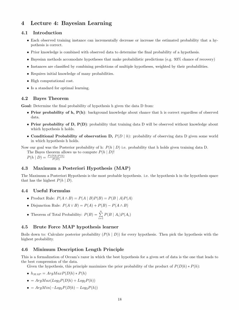
4.2 Bayes Theorem

Goal: Determine the final probability of hypothesis h given the data D from:

• Prior probability of h, P(h): background knowledge about chance that h is correct regardless of observeddata.

• Prior probability of D, P(D): probability that training data D will be observed without knowledge aboutwhich hypothesis h holds.

• Conditional Probability of observation D, P (D | h): probability of observing data D given some worldin which hypothesis h holds.

Now our goal was the Posterior probability of h: P (h | D) i.e. probability that h holds given training data D.The Bayes theorem allows us to compute P (h | D)!

P (h | D) = P (D|h)P (h)P (D)

4.3 Maximum a Posteriori Hypothesis (MAP)

The Maximum a Posteriori Hypothesis is the most probable hypothesis. i.e. the hypothesis h in the hypothesis spacethat has the highest P (h | D).

4.4 Useful Formulas

• Product Rule: P (A ∧B) = P (A | B)P (B) = P (B | A)P (A)

• Disjunction Rule: P (A ∨B) = P (A) + P (B)− P (A ∧B)

• Theorem of Total Probability: P (B) =n∑i=1

P (B | Ai)P (Ai)

4.5 Brute Force MAP hypothesis learner

Boils down to: Calculate posterior probability (P (h | D)) for every hypothesis. Then pick the hypothesis with thehighest probability.

4.6 Minimum Description Length Principle

This is a formalization of Occam’s razor in which the best hypothesis for a given set of data is the one that leads tothe best compression of the data.

Given the hypothesis, this principle maximizes the prior probability of the product of P (D|h) ∗ P (h):

• hMAP = ArgMaxP (D|h) ∗ P (h)

• = ArgMax(Log2P (D|h) + Log2P (h))

• = ArgMin(−Log2P (D|h)− Log2P (h))

18

4.7 Bayes Optimal Classifier

Another problem is the following: Given data D, hypothesis space H, and a new instance x, what is the most probableclassification of x? It is not the most probable hypothesis in H. The Bayes optimal classifier assigns to an instancethe classification cj that has the maximum posterior probability P (cj | D). Now the maximum posterior probabilityP (cj | D) is calculated using the theorem for total probability. It is calculated using all the hypotheses weighted bytheir posterior probabilities w.r.t. the data D:

vOB = arg maxcj∈{+,−}P (cj | D)= arg maxcj∈{+,−}

∑hi∈H

P (cj | hi)P (hi | D)

Best classification method according to its average accuracy. However the bayes optimal classifier may not be inthe hypothesis space!

4.8 Gibbs Classifier

1. Choose hypothesis at random according to P (h | D)

2. Use this hypothesis to classify new instance

Actual error: E[errorGibbs] ≤ 2E[errorBayesOptimal]

4.9 Naıve Bayes Classifier

Given attributes a ∈ A and values v ∈ V, calculate the maximum probability for values Vi such that:

• vMAP = arg max P (Vj)∏i

P (ai | vj)

It assumes that attributes are conditionally independent!

To estimate the probability P (A = v | C) of an attribute-value A = v for a given class C we use:

• Relative Frequency: i.e. nCn where nC is the number of instances that belong to class C and have value v

for the attribute A, and n is the number of training instances of the class C.

• M-estimate of accuracy nc+mpn+m where p is the prior probability of P (A = v | C) and m is the weight of p.

We take the normalized probability of the outcomes of the above, and the one with the higher probability is theone that is classified as positive.

19

5 Lecture 5: Linear Regression

TL;DR

Linear regression is the act of trying to define a function Y given an input vector X based on the values x ∈ X thatbest describe the patterns of X. We usually do this by finding the least-square error between data point x and theapproximated function Y, or by minimizing a penalized version of the least squares loss function.

5.1 Supervised Learning: Regression

Linear regression models the relationship between a scalar dependent variable y and one or more explanatory variables(or independent variables) denoted X. The case of one explanatory variable is called simple linear regression. Formore than one explanatory variable, the process is called multiple linear regression.

In linear regression, the relationships are modeled using linear predictor functions whose unknown model param-eters are estimated from the data. Such models are called linear models. Most commonly, the conditional mean of ygiven the value of X is assumed to be an affine function of X ; less commonly, the median or some other quantile ofthe conditional distribution of y given X is expressed as a linear function of X. Like all forms of regression analysis,linear regression focuses on the conditional probability distribution of y given X .

5.1.1 Regression versus Classification

When do we consider a problem as a classification or regression problem? A classification problem is for identifyingindividual cases (true or false, 0 or 1) whereas regression problems deal with predicting (continuous) amounts/valuesfor products.

5.2 Linear Regression

Given a training set of values (vector) X, apply a learning algorithm and try to learn a hypothesis h, represented asa linear function where h is a function that maps x values to y results:

• y = hΘ(x) = Θ0x0 + Θ1x1...Θnxn for every decision variable xi where ( 0 ≤ i ≤ n).

Except how do we calculate the parameters Θ?

5.3 Cost function intuition

We want to choose Θ0,Θ1 such that hΘ(x) is close to y for our training examples (x, y). The idea behind the costfunction is that we want to minimize the total distance between the (estimation) line and the training data. Whenminimizing the cost, we often normalize by m so that we can view the cost function as an approximation of the”generalization error,” or the expected square loss on a randomly chosen new example. Put more simply, we areminimizing the error rate instead of the total error. For models with 1 variable:

• Hypothesis:

– hΘ(x) = Θ0 + Θ1x

• Parameters:

– Θ0,Θ1

• Cost Function J(Θ0,Θ1):

– J(Θ0,Θ1) = 12m

m∑i=1

(hΘ(x(i))− y(i))2, where:

– hΘ(x(i))− y(i)

is the minimized difference between the calculated result and the actual test data. To find out optimal values forthe parameters Θ0 and Θ1 we want to minimize the difference between the calculated result and the actual result ofour test data.

We attach the coefficient 12 to prevent the square 2 from having an effect on the resulting derivative. We also

divide by the number of summands m to get the average cost per data point.

20

The error measure in the cost function is a ”statistical distance”; in contrast to the popular and preliminaryunderstanding of distance between two vectors in Euclidean space. With statistical distance we are attempting tomap the ”dis-similarity” between estimated model and optimal model to Euclidean space.

There is no constricting rule regarding the formulation of this statistical distance, but if the choice is appropriatethen a progressive reduction in this ’distance’ during optimization translates to a progressively improving modelestimation. Consequently, the choice of ’statistical distance’ or error measure is related to the underlying datadistribution.

21

5.3.1 Least Squares Error

Given a collection of data points (xi, yi) once you have your hypothesis h for some Θ, your least squares error of hon a single data point Θ is:

• (hΘ(xi)− yi)2

If we sum up the errors for all Θ, we multiply by 12 to prevent the square 2 from having an effect on the derivative,

resulting in the total error:

• 12

m∑i=1

(hΘ(x(i))− y(i))2

We also divide the total error by the number of summands m to get the average error per data point, givingus the resulting coefficient of 1

2m .

• 12m

m∑i=1

(hΘ(x(i))− y(i))2

When comparing performance on two data sets of different size, the raw sum of squared errors are not directlycomparable because larger data sets tend to lead to higher error totals. When you normalize, you can comparethe average error per data point.

5.4 Gradient descent

Gradient Descent is a very well-known algorithm for finding maxima and minima, however it can get stuck in localities(local minimum). It is used in all sorts of optimization problems, not just regression. It is relatively simple comparedto other more sophisticated techniques, yet is still useful.

Gradient Descent is an iterative algorithm for finding max/min of a function:

1. Start with some Θ0,Θ1

2. Keep updating Θ0,Θ1 to reduce J(Θ0,Θ1) until you (hopefully) reach a minimum.

Mathematically:

1. hΘ(x) = Θ0 + Θ1x

2. J(Θ0,Θ1) = 12m

m∑i=1

(hΘ(x(i))− y(i))2

3. Θ0 := Θ0 − α( 12m

m∑i=1

(hΘ(x(i))− y(i))2) (repeat until convergence)

where m is the no. of data points and α is the learning rate. (Usually pre-defined)

5.4.1 Choosing Learning Rate

We don’t want the learning rate α to be too small or too big:

• Too small: Slow convergence

• Too big: gradient step may overshoot (and thus we do not converge, leading to an endless loop)

5.4.2 Multiple Features

Gradient descent can also be used for multivariate linear regression, where the cost function would be:

• J(Θj) = hΘ(x) = Θ0 + Θ1x1 + Θ2x2 + ...+ Θnxn

and the gradient descent algorithm would look like this:Repeat until converged :

1. Θj := Θj − α 1m

m∑i=1

(hΘ(x(i))− y(i))x(i)j

NOTE: Simultaneously update every Θj! Only after updating ALL Θ’s should you update hΘ(x)!

22

5.5 Normal Equation

5.5.1 Feature Scaling

With feature scaling we get all features in the [-1, 1] range. Basically what we do is we standardize the range ofindependent variables or features of data, because scaling ensures that if some feature values are large it won’t leadto them being used as a main predictor. This may optimize performance for the gradient descent algorithm and isknown as the normal equation.

5.5.2 The Algorithm

The normal equation is performed as follows:

• we’ll have to minimize for Θ: 12 [XΘ− y]T [XΘ− y] which effectively boils down to:

• XTXΘ−XT y and then setting the gradient to zero:

• XTXΘ = XT y from which follows that:

• Θ = (XTX)−1XT y - note: the -1 means matrix inversion here.

5.6 Normal Equation vs Gradient Descent

• Gradient Descent

– Need to choose α

– needs many iterations

– works well even when the number of features is large

• Normal Equation

– No need for α

– No need to iterate

– Needs to compute (XTX)−1

∗ O(n3)

∗ might be non-invertible

5.7 Finding the ”right” model

There are 2 problems that we are facing, overfitting and underfitting. This can be solved by one of the following:

1. Reducing the number of features.

• Manually select which features to keep

• Model selection algorithm

2. Regularization

• Keeps all the features but reduces the magnitude of parameters Θj .

• Works well when we have a lot of features, each of which contributes a bit to predicting y.

5.7.1 Regularization

When applying regularization we alter the cost function into the following:

• J(Θ) = 12m [

m∑i=1

(hΘ(x(i))− y(i))2 + λn∑j=1

Θ2j ] Where the regularization term we add is: λ

n∑j=1

Θ2j ]

Regularization parameter λ is an input parameter to the model. Lambda can be selected by sub-sampling thedata and finding the variation. The value of lambda can reduce overfitting as it increases, however it doesthis at the expense of greater bias.

23

For the gradient descent algorithm it would look as follows:

• Θj := Θj − α[ 1m

m∑i=1

(hΘ(x(i))− y(i))x(i)j + λ

mΘj ], then

• Θj := Θj(1− α λm )− α[ 1

m

m∑i=1

(hΘ(x(i))− y(i))x(i)j ]

For the normal equation:

Θ = (XTX + λ

0 0 0 0 00 1 0 0 00 0 1 0 00 0 0 ... 00 0 0 0 1

−1

XT y

Two advantages:

1. Fights over-fitting

2. Guarantees matrix of full rank, and thus invertible

24

6 Lecture 6: Logistic Regression and Artificial Neural Networks

6.1 Logistic Regression

We can cast a binary classification problem into a continuous regression problem. However we can not simply use thelinear regression that we mentioned before. Logistic regression is used when the variable y that we want to predictcan only take on discrete values (i.e. Classification). Considering a binary classification problem (y = 0 or y = 1),the hypothesis function could be defined so that it is bounded between [0, 1] in which we use some form of logisticfunction, such as the Sigmoid Function. Other, more efficient functions exist such as the ReLU (Rectified LinearUnit), however there are not covered in this course as the sigmoid function is a historical standard.

6.1.1 Sigmoid Logistic Regression

One option is to use a sigmoid function. Why? Because it allows hΘ(x) to only have values between 0 and 1. Thismeans a more fluent transition is made from false to true.

Sigmoid function:

• g(x) = 11+e−z

Now for the hypothesis:

• hΘ(x) = g(ΘTx) = 1

1+e−ΘT x

The decision boundary for the logistic sigmoid function is where hΘ(x) = 0.5 (values less than 0.5 means false,values equal to or more than 0.5 means true). Another interesting property is that it also gives a chance of the instancebeing of that class e.g. hΘ(x) = 0.7 means that there is a 70% chance that the instance is of the corresponding class,so we get:

• hΘ(x) = g(Θ0 + Θ1x1 + Θ2x2) and we predict y=1 if:

• −3 + x1 + x2 ≥ 0

6.1.2 Non-Linear Decision Boundaries

Now in the above cases of logistic regression we are speaking of a linear decision boundary (meaning we can drawa straight line between the class and other instances. However sometimes this is not the case. When dealing withnon-linear decision boundaries we use higher order polynomials in order to be able to classify these cases, e.g.:

• hΘ(x) = g(Θ0 + Θ1x1 + Θ2x2 + Θ3x21 + Θ4x

22) and we predict y=1 if:

• −1 + x21 + x2

2 ≥ 0

6.2 Cost Function

Given a new hypothesis, we now need a cost function. However, just by using the sigmoid function, we end up witha non-convex cost function. This means that local minima are found must faster than the global minimum, andleads to slow or incorrect learning.

• J(Θ0,Θ1) = 12m

m∑i=1

Cost(hΘ, y) where

• Cost(hΘ, y) is 12 (hΘ(x)− y)2

However, by using the sigmoid function, we end up with a non-convex cost function. This means that localminima are found must faster than the global minimum, and leads to slow or incorrect learning.

Cost(hΘ(x), y) =

{−log(hΘ(x)), if y = 1

−log(1− hΘ(x)), if y = 0

This means that the optimization objective function can be defined as the mean of the costs/errors in thetraining set:

• J(Θ) = 1m

m∑i=1

Err(hΘ(x(i), y(i))

25

6.3 Gradient Descent for Logistic Regression

How do we find the right Θ parameter value? We use gradient descent!

• Repeat until convergence:

1. Θj := Θj − α[

1m

m∑i−1

(hΘ(x(i))− y(i))x(i)j

]NOTE: Simultaneously update all Θj!Looks identical to linear regression but with hΘ(x) = 1

1+e−ΘT xand with regularization:

Repeat until convergence:

1. Θj := Θj − α δδΘj

J(Θ), or:

(a) δδΘ0

J(Θ) = 1m

m∑i=1

(hΘ(x(i))− y(i))x(i)0

(b) δδΘ1

J(Θ) = 1m

m∑i=1

(hΘ(x(i))− y(i))x(i)1 + λ

mΘ1

(c) δδΘ2

J(Θ) = 1m

m∑i=1

(hΘ(x(i))− y(i))x(i)1 + λ

mΘ2 ...

6.4 Multi-Class Problems

Simply make k copies of ”One vs All”. When predicting pick the class with the highest probability (highest outcomeof hΘ).

6.5 Artificial Neural Networks

Artificial neural networks (ANNs) are computing systems inspired by the biological neural networks that constituteanimal brains. Such systems learn (progressively improve performance on) tasks by considering examples, generallywithout task-specific programming. An ANN is based on a collection of connected units or nodes called artificialneurons (analogous to biological neurons in an animal brain). Each connection (synapse) between neurons cantransmit a signal from one to another. The receiving (postsynaptic) neuron can process the signal(s) and then signalneurons connected to it.

In common ANN implementations, the synapse signal is a real number, and the output of each neuron is calculatedby a non-linear function of the sum of its inputs. Neurons and synapses typically have a weight that adjusts as learningproceeds. The weight increases or decreases the strength of the signal that it sends across the synapse. Neurons mayhave a threshold such that only if the aggregate signal crosses that threshold is the signal sent.

Typically, neurons are organized in layers. Different layers may perform different kinds of transformations ontheir inputs. Signals travel from the first (input), to the last (output) layer, possibly after traversing the layersmultiple times. Alternative architectures include :

• Recurrent Networks (gives memory effect (e.g. counting, adding etc.)

• Multi class Problems

6.5.1 Forward Propagation

With Neural Networks, we’re trying to find a minimum of some certain function, where each neuron is connected toall other neurons in the previous layer, where the weights in the weighted sum are acting like the strength of each ofthose connections. The bias is some indication whether that specific neuron tends to be active or inactive.

• a(j)i = ”activation” of unit i in layer j:

• Θ(j) = matrix of weights controlling function mapping from layer j to layer j+1. It has dimension sj+1by(sj+1)where sj is the number of nodes on layer j

26

so:

• a(2)1 = g(Θ

(1)10 x0 + Θ

(1)11 x1 + Θ

(1)12 x2)

• a(2)2 = g(Θ

(1)20 x0 + Θ

(1)21 x1 + Θ

(1)22 x2)

• hΘ(x) = g(Θ(2)10 a

(2)0 + Θ

(2)11 a

(2)1 + Θ

(2)12 a

(2)2 )

6.5.2 Learning The Weights

Back propagation; uses gradient descent similar to lin. & log. regression. Where do we get errors for internal nodes?It is given that d

dxg(x) = g(x)(1− g(x)) and we can back propagate as follows:Algorithm for learning the weights:

Training set {((x(1), y(1)), ..., (x(m), y(m)) } Set ∆(l)ij = 0 (for all l, i, j)

For i = 1 to m {set a(1) = x(i)

Set a(1) = x(i)

Perform forward propagation to compute a(l) for l = 2,3,...,LUsing y(i), compute δ(L) = a(L) − y(i)

Compute δ(L−1), δ(L−2), ..., δ(2)

∆(l)ij := ∆

(l)ij + a

(l)j δ

(l+1)i

}D

(l)ij := 1

m [∆(l)ij + λΘ

(l)ij ] if j 6= 0

D(l)ij := 1

m [∆(l)ij if j = 0

δ

δΘ(l)ij

J(Θ) = D(l)ij

6.5.3 Properties Of Neural Networks

• Useful for modelling complex, non-linear function of numerical inputs and outputs

– symbolic inputs/outputs represented using some encoding

– 2 or 3 layer networks can approximate a huge class of functions (if enough neurons in hidden layers)

• Robust to noise; but risk of over fitting (due to high expressiveness)! e.g. training for too long. Usually handledusing validation sets.

• All inputs have some effect: Decision trees: selection of most important attribtutes, ANN ”Selects” attributesby giving them higher/lower weights

• Explanatory power of ANNs is limited

– Model represented as weights in network

– No simple explanation why network makes a certain prediction (cf. trees can give a rule that was used)

– Networks can not easily be translated into a symbolic model (tree, ruleset)

Use ANNs when:

• High dimensional input and output (numeric or symbolic)

• Interpretability of model unimportant

27

7 Lecture 7: Recommender Systems

7.1 Collaborative Filtering

In short what this means is that we look at what other users/customers liked/rated and try to use this informationto recommend other products.

7.2 Content Based Approach

Given a list of films:

Movie Θ(1) Alice(1) Θ(2) Bob(2) Carol(3)Love at last 5 5 0 0

Romance Forever 5 ? ? 0Cute puppies of Love ? 4 0 ?

Nonstop car chases 0 0 5 4Swords vs. karate 0 0 5 ?

• Now the Optimization Criterion: To learn Θ(j) (parameter for user j)

– minΘ(j)12

∑i:r(i,j)=1

((Θ(j))Tx(i) − y(i,j)

)2+ λ

2

n∑k=1

(Θ(j)k )2

• Now in order to learn all parameters (Θ(1),Θ(2), ...,Θ(nu):

– minΘ(1),...,Θ(nu )12

nu∑j=1

∑i:r(i,j)=1

((Θ(j))Tx(i) − y(i,j)

)2Note: the 2nd formula combines the knowledge from all users!

• So now we can update the gradient descent algorithm for this case:

– Θ(j)k := Θ

(j)k − α

( ∑i:r(i,j)=1

((Θ(j))Tx(i) − y(i,j))x(i)k

)for k = 0

– Θ(j)k := Θ

(j)k − α

( ∑i:r(i,j)=1

((Θ(j))Tx(i) − y(i,j))x(i)k + λΘ

(j)k

)for k 6= 0

7.3 Collaborative Filtering

Given x(1), ..., xnm estimate Θ(1), ...,Θ(nu):

• minΘ(1),...,Θ(nu)12

nu∑j=1

∑i:r(i,j)=1

((Θ(j))Tx(i) − y(i,j)

)2+ λ

2

nu∑j=1

n∑k=1

(Θ(j)k )2

Given Θ(1), ...,Θ(nu) estimate x(1), ..., x(nm):

• minx(1),...,x(nm)12

nm∑j=1

∑j:r(i,j)=1

((Θ(j))Tx(i) − y(i,j)

)2+ λ

2

nm∑j=1

n∑k=1

(x(i)k )2

Estimating x(1), ..., xnm and Θ(1), ...,Θ(nu) simultaneously:

• J(x(1), ..., x(nm),Θ(1), ...,Θ(nu)) =

12

∑(i,j):r(i,j)=1

((Θ(j))Tx(i) − y(i,j))2 + λ2

nm∑i=1

n∑k=1

(x(i)k )2 + λ

2

nu∑j=1

n∑k=1

(Θ(j)k )2

28

7.3.1 Collaborative Filtering Algorithm

1. Initialize the input featuers x(1), ..., xnm , and weights Θ(1), ...,Θ(nu) to small random values.

2. Minimize the cost function J(x(1), ..., xnm ,Θ(1), ...,Θ(nu)) using gradient descent (or another optimization al-gorithm).

3. For a user with (learned) parameter Θ and a movie with (learned) features x, predict a star rating of ΘTx.

7.3.2 Mean Normalization

Brand new users will receive a prediction of 0 (not very useful). In order to avoid this we can normalize themean. What we do is, we calculate the average rating, and we normalize by subtracting the average rating from theset of ratings that each existing user has given so far. Then for user j, on movie i predict: (Θ(j))T (x(i)) + µi So ifthere is no information from a user we give recommendations equal to the average rating!

7.4 Support Vector Machines

Usable in similar situations as neural networks. Important concepts:

• Finding a ”maximal margin” separation.

• Transformation into high dimensional space.

7.4.1 Linear SVMs

The idea is to find a hyperplane that discriminates + from - where the margin/distance of hyperplane to closestpoints is maximal. The solution is unique and determined by just a few points (Support vectors).

7.4.2 Non-Linear SVMs

1. Transfrom data to a higher-dimensional space where they are hopefully linearly separable.

2. Learn linear SVM in that space.

3. Transform linear SVM back to original space.

7.4.3 Logistic Regression to SVM

Alternative view on logistic regression:

• Cost of example: −(y log hΘ(x) + (1− y) log(1− hΘ(x))) = −y log 1

1+e−ΘT x− (1− y)log(1− 1

1+e−ΘT x)

This can be done for similar reasons why we would use logistic regression in other classification cases.

7.4.4 Kernels

Pick data points in the space (named landmarks). Idea is that by applying a positive or negative weight to thedistance to a data point/kernel we can predict whether or not a new instance is a class:

• predict y = 1 if:

– Θ0 + Θ1f1 + Θ2f2 + ...+ Θifi ≥ 0

• given x:

– fi = similarity(x, l(i)) = exp(− ||x−l(i)||2

2δ2 ) where l(i) is kernel i

29

7.4.5 Cost Function

Hypothesis: Given x, compute features f ∈ Rm+1:

• predict ”y=1” if ΘT f ≥ 0

Training:

• minΘ Cm∑i−1

y(i)cost1(ΘT f (i)) + (1− y(i))cost0(ΘT f (i)) + 12

n∑j=1

Θ2j

7.5 Compare SVM

It is interesting to comapre SVM with:

• Multi-layered Neural Networks:

– Perceptron: linear separation, not with maximal margin.

– ANN obtains better expressiveness by changing representation throughout its layers.

– SVM obtains better expressiveness through non-linear transformation.

• Instance Based Learning:

– SVM stores examples that identify boundary between classes; classification based on which side of theboundary new example is.

– IBL: stores all examples; classification based on distance to stored examples.

30

8 Lecture 8:

8.1 Nearest Neighbor Algorithm

Idea: Instances that lie ”close” to each other are most likely similar to each other.

8.1.1 Properties

• Learning is very fast

• No info is lost (brings disadvantage: ”Details” may be noisy)

• Hypothesis space:

– Variable size

– Complexity of the hypothesis rises with the number of stored examples

8.1.2 Decision Boundaries

The sample space is basically ”cut” into pieces for all data points. These boundaries are not computed!So in essence we keep all information. However this comes with the problem that more details means more noise.

In order to improve robustness against noisy learning examples we use a set of nearest neighbors. For classificationwe use voting, and for regression we use the mean.

The method in the book contains a mistake, see the slide about the book.

8.1.3 Lazy vs Eager Learning

Lazy learning: Don’t do anything until we need to make a prediction (e.g. Nearest Neighbor)

• Learning is fast

• Predictions require work and can be slow

Eager learning: Start computing as soon as we receive data. (Decision tree, neural networks etc.)

• Learning can be slow

• predictions are usually fast!

8.1.4 Inductive vs Transductive learning

Induction: for input x find a model/function to calculate y.

• Computations take only learning data into account

• a single model must work well for all new data: global model

Transduction: for input x find some output y

• computations can take extra info about the needed predictions into account.

• Can use local models that work well in the neighborhood of the target example.

8.1.5 Semi-Supervised Learning

The learner gets a set of labeled data and a set of unlabeled data. Information about the probability distribution ofexamples can help the learner. Seen the little info on the slides this is probably not important.

31

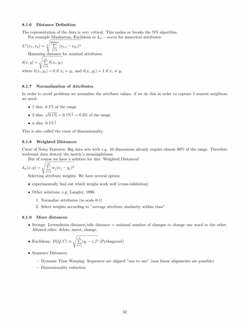
8.1.6 Distance Definition

The representation of the data is very critical. This makes or breaks the NN algorithm.For example Manhattan, Euclidean or Ln − norm for numerical attributes:

Ln(x1, x2) = n

√#dim∑i=1

|x1,i − x2,i|n

Hamming distance for nominal attributes:

d(x, y) =

√n∑i=1

δ(xi, yi)

where δ(xi, yi) = 0 if xi = yi, and δ(xi, yi) = 1 if xi 6= yi

8.1.7 Normalization of Attributes

In order to avoid problems we normalize the attribute values. if we do this in order to capture 5 nearest neighborswe need:

• 1 dim: 0.1% of the range

• 2 dim:√

0.1% = 0.1%12 = 0.3% of the range

• n dim: 0.1%1n

This is also called the curse of dimensionality.

8.1.8 Weighted Distances

Curse of Noisy Features: Big data sets with e.g. 10 dimensions already require almost 60% of the range. Thereforeirrelevant data destroy the metric’s meaningfulness.

But of course we have a solution for this: Weighted Distances!

dw(x, y) =

√D∑j=1

wj(xj − yj)2

Selecting attribute weights. We have several option:

• experimentally find out which weighs work well (cross-validation)

• Other solutions, e.g. Langley, 1996:

1. Normalize attributes (to scale 0-1)

2. Select weights according to ”average attribute similarity within class”

8.1.9 More distances

• Strings: Levenshtein distance/edit distance = minimal number of changes to change one word to the other.Allowed edits: delete, insert, change.

• Euclidean: D(Q,C) ≡√

n∑i=1

(qi − ci)2 (Pythagoras!)

• Sequence Distances:

– Dynamic Time Warping: Sequences are aligned ”one to one” (non linear alignments are possible)

– Dimensionality reduction

32

8.2 Distance-weighted kNN

Idea: give higher weight to closer instances so we can now use all training instances instead of only k aka ”Shepard’smethod”.

• f(xq) =

k∑i=1

wif(xi)∑ki=1 wi

with wi = 1d(xq,xi)2

This results in a fast learning algorithm but it has slow predictions. Efficiency:

• for each prediction, kNN needs to compute the distance for ALL stored examples.

• Prediction time = linear in the size of the data set, for large training sets and/or complex distances this canbe too slow to be practical.

8.2.1 Edited k-nearest neighbor

• Less storage (good).

• Order dependent (bad).

• Sensitive to noisy data (bad).

• More advanced alternatives exist (= IB3).

The algorithm:Incremental Deletion of ExamplesEdited k-NN(S) S: Set of instancesFor each instance x in S if x is correctly classified by S\x

Remove x from SReturn S

Incremental addition of examples Edited k-NN(S) S: Set of instancesT = ∅For each instance x in S

if x is not correctly classified by TAdd x to T

Return T

8.3 Pipeline Filters

Pipeline filters: Reduce time spent on far-away examples by using more efficient distance-estimates first. We caneliminate most examples using rough distance approximations and compute more precise distances for examples inthe neighborhood.

8.4 kD-trees

kD-trees: use a clever data structure to eliminate the need to compute all distances. kD-trees are similar to decisiontrees except:

• Splits are made on the median/mean value of dimension with highest variance

• Each node stores one data point, leaves can be empty

Finds closest neighbor in logarithmic (depth of tree) time. However building a good kD-tree may take some time:Learning time is no longer 0 and incremental learning is no longer trivial:

• kD-tree will no longer be balanced

• re-building the tree is recommended when the max depth becomes larger than 2 * the minimal required depth(= log(N) with N training examples).

33

Using Prototypes: the rough decision surfaces of nearest neighbor can sometimes be considered a disadvantage. Wecan solve two problems at once by using prototypes (= representative for a whole group of instances) For exampleprototypes can be:

• single instances, replacing a group

• other structure, (e.g., rectangle/shape, rule, ..)

• Radial basis function networks Basically builds a global approximation as linear combination of local approxi-

mations. f(x) = w0 +k∑u=1

wuKu(d(xu, x))

A common choice for Ku(d(xu, x)) = e−1

2δ2ud2(xu,x)

. by using this the influence of each local approximation ugoes down quickly with distance.

8.5 Local Learning

• Collect k nearest neighbors

• Give them a supervised algorithm

• Apply learned model to test example

Locally weighted Regression Build local model in region around x (e.g. linear or quadratic model). Minimiz-ing:

• squared error for k neighbors: E1(xq) ≡∑

x∈kNN(xq)

(f(x)− f(x))2.

• Distance-weighted squared error for all neighbors: E2(xq) ≡∑x∈D

(f(x)− f(x))2K(d(xq, x))

8.6 Comments on k-NN

Positive

• Easy to implement

• Good ”baseline” algorithm / experimental control

• Incremental learning easy

• Psychologically plausible model of human memory

Negative

• Led astray by irrelevant features

• No insight into domain (no explicit model)

• Choice of distance function is problematic

• Doesn’t exploit/notice structure in examples

8.7 Decision Boundaries

Basically tries to make a partition (of as few divisions as possible) of the version space that indicates for each partitionto what class it belongs.

8.8 Sequential Covering Approaches

Also known as the ”Separate and Conquer” approach. General principle: Learn a rule set one rule at a time. It triesto learn one rule that has a high accuracy (when it predicts something, it should be correct) and any coverage (doesnot make a prediction for all examples just for some of them). Then mark the covered examples (these have beentaken care of; now focus on the rest). Repeat until all examples covered.

34

8.8.1 Candidate Literals

There are two separate methods to determining candidate literals for these algorithms.

Top-Down Learn One Rule

For this algorithm, we simply go through all of the possible combinations of categories and their values, i.e. (wind =weak), (wind = strong), (temp = mild), (temp = cool), (humidity = normal), (humidity = high) are all the possiblecandidate literals for the above algorithm from the example in the homework assignment.

Top-down Example-driven Learn One Rule

For this algorithm, we want to find the literals that have the highest accuracy. First, we select an arbitrary examplee (usually starting with e1) and we find out which literal value has the highest accuracy. For example, if (humidity= normal) has accuracy of 3

4 , we count that as our first literal. However, because the accuracy is not 100%, we mustfind a second example such that (hum = norm) AND (literal #2) have 100% accuracy.

In the example in the homework, when (temp = mild) it has 23 positive cases, where 2

2 are covered when inconjunction with (hum = norm). Therefore, the first rule is:

1. IF (hum = norm) AND (temp = mild)

which covers e1 and e2. However, this does not cover all positive cases. There still exists a third positiveexample (e3). In this example, when (wind = weak) there are 2

2 positive examples. Since when (wind = weak)we cover all remaining positive examples (e3), which leads to the conclusion that the second rule is:

2. IF (wind = weak)

and we are done.

8.8.2 Sequential covering

function LearnRuleSet(Target, Attrs, Examples, Threshold):LearnedRules:= ∅Rule:= LearnOneRule(Target, Attrs, Examples)while performance(Rule,Examples) > Threshold, do

LearnedRules := LearnedRules⋃{Rule}

Examples := {Examples} \ {examples classified correctly by Rule}Rule := LearnOneRule(Target, Attrs, Examples)

Optional: Sort learned rules according to performancereturn LearnedRules

Learning One Rule

• Perform greedy search

• Could be top-down or bottom-up

– Top-down:

∗ Start with maximaly general rule (has maximal coverage but low accuracy)

∗ Add literals one by one

∗ Gradually maximize accuracy without sacrificing coverage (using some heuristic)

Top down has typically more general rules

– Bottom-up:

∗ Start with maximally specific rule (has minimal coverage but maximal accuracy)

∗ Remove literals one by one

∗ Gradually maximize coverage without sacrificing accuracy (using some heuristic)

Bottom up has typically more specific rules

35

8.8.3 Heuristics

When is rule considered a good rule?

• High accuracy

• High coverage (less important than accuracy)

Possible evaluation functions:

• Accuracy: pp+n where p=# positives, n=# negatives

• Variant on Accuracy: m-estimate: p+mqp+n+m . Weighted mean between accuracy on covered set of examples and

a priori estimate of true accuracy q (m is weight).

• Entropy: more symmetry between positive and negative

8.9 Example-driven Top-down Rule induction

Idea: for a given class c:As long as there are uncovered examples for C

• pick one such example e

• consider He = rules that cover this example

• search top-down in He to find best rule

Much more efficient search (He much smaller than H (set of all rules).Less robust with respect to noise; noisy example may require a restart.

8.10 Avoiding over-fitting

Post-pruning:

1. Split instances into Growing Set and Pruning Set

2. Learn set SR of rules using Growing Set

3. Find the best simplification BSR of SR

4. while(Accuracy(BSR, Pruning Set) ¿ Accuracy(SR, Pruning Set)) do

(a) SR = BSR

(b) Find the best simplification BSR of SR

5. return BSR

36

9 Lecture 9: Clustering

9.1 Unsupervised Learning

Data just contains x, there is no given classification or other information. The main goal is to find structure in thedata. The definition of ground truth is often missing (no clear error function like in supervised learning.

9.2 Clustering

Problem definition:Let X = (x1, x2, ..., xd) be a d-dimensional feature vector.Let D be a set of vectors, D = X1, X2, ..., Xn Given data D, group the N vectors into K groups such that thegrouping is optimal.

Clustering is used for:

• Establish prototypes or detect outliers

• Simplify data for further analysis/learning

• Visualize data

• Preprocessing step for algorithms

• stand alone tool to get insight into data distribution

A good clustering method will produce clusters with

• High intra-class similarity

• Low inter-class similarity

• precise definition of clustering quality is difficult (application-dependent and ultimately subjective)

9.3 Similarity Measures

Possible options

• Distance Metric (Ln metric, ...)

• More general forms of similarity (Do not necessarily satisfy triangle inequality, symmetry, ...)

9.4 Flat vs. Hierarchical Clustering

Flat clustering: Given data set, return partition Hierarchical Clustering:

• Combine clusters into larger clusters, etc. until 1 cluster = full data set

• Gives rise to cluster hierarchy or taxonomy (taxonomy = grouping of classes; e.g. mammals - Felines - Tigersetc.)

9.5 Extensional vs Intensional Clustering

Extensional clustering: Clusters are defined as sets of examples. Intensional clustering Clusters described insome language. Typical criteria for good intensional clustering:

• High intra cluster similarity

• Simple conceptual description of clusters.

37

9.6 Cluster Assignment

• Hard clustering: Each item is a member of one cluster

• Soft Clustering: Each item has a probability of membership in each cluster

• Disjunctive clustering: An item belongs to only one cluster

• An item can be in more than one cluster

• Exhaustive clustering: Each item is a member of a cluster

• Partial Clustering: Some items do not belong to a cluster (in practice this is equal to exhaustive clusteringwith singleton clusters)

9.7 Major Clustering Approaches

• Hierarchical: Create a hierarchical decomposition of the set of objects using some criterion

• Partitioning: Construct various partitions and then evaluate them by some criterion

• Model-based: Hypothesize a model for each cluster and find best fir of models to data

• Density based: Guided by connectivity and density functions

9.8 Hierarchical Clustering

Can do top-down (devisive) or bottom-up (agglomerative). In either case we maintain a matrix of distance (orsimilarity) scores for all pairs of instances, clusters (formed so far) or both.

9.8.1 Dendogram

Tree view on hierarchical clusters; how higher the topbar is (horizontal line) the higher the degree of difference withincluster.

9.8.2 Bottom up Hierarchical Clustering

Given: instances x1, ..., xnfor(i=1 to n) ci = {xi}C = {c1, ..., cn}j = nwhile size of C ≥ 1

j = j+1(ca, cb) = argminu,vdist(cu, cv)cj = ca

⋃cv

add node to tree joining a and bC = C \{ca, cb} ∪ cj

Return tree with root node j

9.9 Distance between two clusters

The distance between two clusters can be determined in several ways

• Single link: Distance of two most similar instances: dist(cu, cv) = min{dist(a, b) | a ∈ cu, b ∈ cv}

• Complete link: distance of 2 least similar instances: dist(cu, cv) = max{dist(a, b) | a ∈ cu, b ∈ cv}

• Average link: average distance between instances: dist(cu, cv) = avg{dist(a, b) | a ∈ cu, b ∈ cv}

Computational complexity: Naive implementation has O(n3) time complexity, where n is the number of instances.More advanced computations:

• Single link: Can update and pick pair in O(n), which results in O(n2) algorithm

• Complete and average link: Can do these steps in O(n log n), which yields an O(n2logn) algorithm.

38

10 Lecture 10:

10.1 Reinforcement learning

Reinforcement learning stems from the situation where an agent only receives a reward after a sequence/series ofactions have been performed. It stems from biological and societal systems where an agent is given a reward (i.e.Dopamine) based on a previous decision(s), instead of given constant guidance towards what is the correct or incorrectdecision.

In reinforcement learning, the agent typically does not possess full knowledge of the environment or the result ofeach action. More formally:

• Given:

1. a Set of States S (known to the agent only after exploration)

2. a Set of Actions A (per state)

3. a Transition function: St = δ(st, at) (unknown to agent) where δ represents the state transition

4. a Reward function: rt = r(st, at) (unknown to agent)

• Find:

1. Policy π : S → A that outputs an appropriate action a from set A, given the current state s from set Ssuch that π(st) = at.

10.2 Optimal Policy

The optimal policy π is found by maximizing the cumulative value/reward:

• V π(st) = rt + γrt+1 + γ2rt+2 + ... ≡∞∑i=0

γirt+i

where gamma 0 ≤ γ ≤ 1 is a ”discount factor” that leads us to prefer either immediate reward or delayed reward(higher values of γ → later reward preference). Therefore, the optimal policy becomes:

• π∗ ≡ ArgMaxaVπ(s), (∀s) where V π

∗is the value function of the optimal policy for state s:

• V π∗(s) or V ∗(s)

However, this demonstrates a problem. How can we learn the optimal policy π∗ : S → A for arbitrary environ-ments? Since training data 〈s, a〉 is not available, π∗ cannot be directly learned because the agent can only directlychoose a and not s. This leads us to the concept of Q-Learning.

10.3 Q-learning Algorithm

Q-learning does not require a model aka it is model-free. It is also exploration-independent (off-policy).

10.3.1 Q-Learning Intuition

We want to maximize the sum of the rewards, doing maximization iteratively while exploring state-action pairs (s,a) to explore the cumulative reward:

• π∗ ≡ ArgMaxa[r(s, a) + γV ∗(δ(s, a))]

The problem with this is that the agent typically does not have perfect knowledge of δ (the state transitions) orr (the reward in all states). This means that agents cannot predict the reward and the immediate successor state→ V ∗ cannot be directly learned directly. Solution - learn the Q-values instead by computing the optimalQ-values for all state-action pairs using the Bellman equation:

• Q(s, a)← r + γmax(α′)Q(s′, a′) so the optimal policy becomes:

• π∗ ≡ ArgMaxaQ(s, a)

39

10.3.2 Learning the Q-Values

We use iterative approximation to learn the Q values for a given state-action pair:

• V ∗ = Maxa′Q(s, a′)

So that we can rewrite:

• Q(s, a) = r(s, a) + γMaxa′Q(δ(s, a), a′)

And we then obtain the recursive update rule that allows an iterative approximation of Q:

• Q(s, a)← r(s, a) +Maxa′Q(s′, a′)

This way, the agent stores the value Q(s, a) in a large look-up table. Then the agent repeatedly observes its owncurrent state s, chooses some action a, and observes the resulting reward r(s, a) and the new state s′ = δ(s, a). Thisway, the agent repeatedly samples from unknown functions δ(s, a) and r(s, a) without having full knowledge of thesefunctions.

10.3.3 Q-Learning Optimality

In deterministic environments (if the next state is perfectly predictable given knowledge of the previous state and theagent’s action), Q-Learning is guaranteed to converge for infinite amounts of updates of each state-actionpair. In practice, infinite amounts of updates are not required to determine the optimal policy.

10.3.4 Accelerating the Q-Learning Process

One way to accelerate this process is to back-propagate the Q-values after a visit of a sequence of states. For thisyou have to remember previously visited states within one run.

In this case, do we choose the next action that maximizesQ(s, a)? NO, because this risks the situation where nonew values are learned and it can become biased by initial random exploration, meaning that Q-Learning wouldnot converge.

The better choice is to balance exploration with the explotation of known Q-values. A probabilistic model:

• P (ai|s) = kQ(s,ai)∑jKQ(s,aj)

Actions with higher Q(s, a) are more likely to be picked compared to other actions. High k = higher exploitationfactor, lower k = higher exploration factor.

10.3.5 Q-Learning Summary

• Q-Learning is model-free: Q-Learning does not need any information about the environment except for the setof valid actions for each state.

• Given a chosen state-action pair, the environment will provide the rewards.

• Once these are given, a reinforcement learning technique such as Q-Learning explores the environment and theconnected reward autonomously and thus performs autonomous learning of the optimal policy.

• Q-Learning is guaranteed to converge given infinite iterations. It however converges in a reasonablenumber of iterations.

10.4 Online Learning and SARSA

An off-policy learner learns the value of the optimal policy independently of the agent’s actions. An on-policylearner learns the value of the policy being carried out by the agent, including the exploration steps.Limitation of off-policy learning: There may be cases where ignoring what the agent actually does is dangerous (therewill be large negative rewards).

SARSA chooses the action that was actually chosen by the agent (rather than the best possible action argmaxQ(s, a)).

• Can take exploration into account

• Online and continuous learning

40

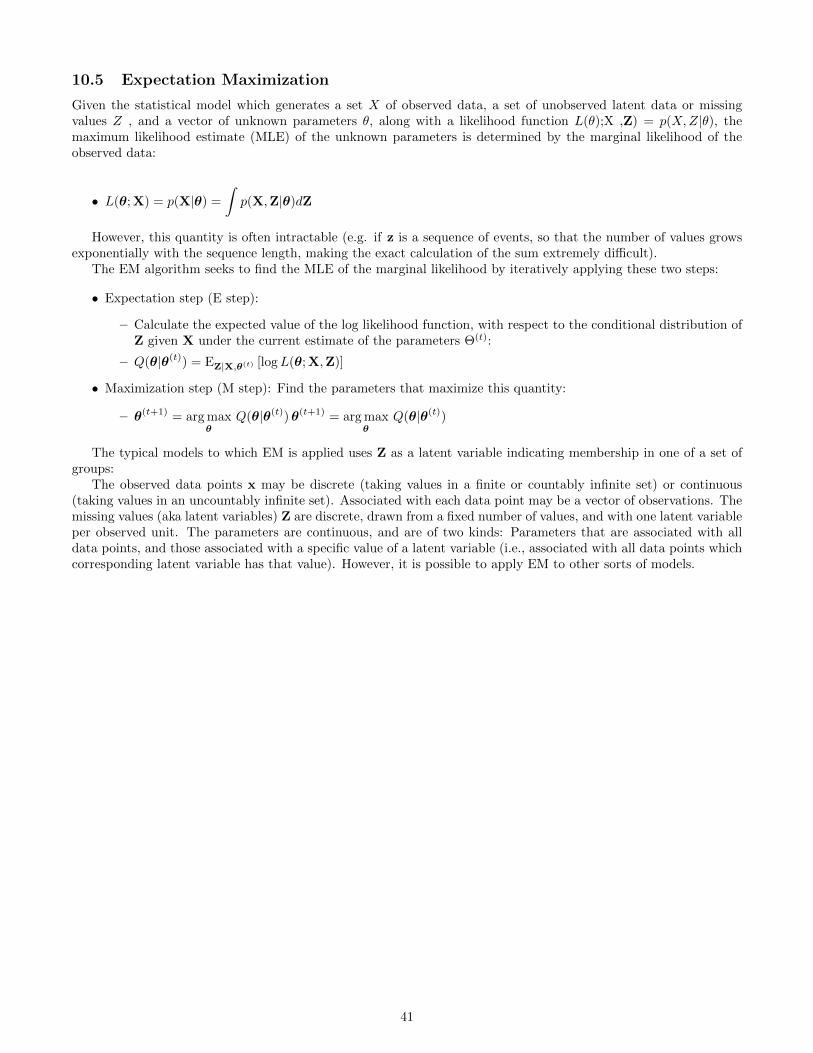
10.5 Expectation Maximization

Given the statistical model which generates a set X of observed data, a set of unobserved latent data or missingvalues Z , and a vector of unknown parameters θ, along with a likelihood function L(θ);X ,Z) = p(X,Z|θ), themaximum likelihood estimate (MLE) of the unknown parameters is determined by the marginal likelihood of theobserved data:

• L(θ; X) = p(X|θ) =

∫p(X,Z|θ)dZ

However, this quantity is often intractable (e.g. if z is a sequence of events, so that the number of values growsexponentially with the sequence length, making the exact calculation of the sum extremely difficult).

The EM algorithm seeks to find the MLE of the marginal likelihood by iteratively applying these two steps:

• Expectation step (E step):

– Calculate the expected value of the log likelihood function, with respect to the conditional distribution ofZ given X under the current estimate of the parameters Θ(t):

– Q(θ|θ(t)) = EZ|X,θ(t) [logL(θ; X,Z)]

• Maximization step (M step): Find the parameters that maximize this quantity:

– θ(t+1) = arg maxθ

Q(θ|θ(t))θ(t+1) = arg maxθ

Q(θ|θ(t))

The typical models to which EM is applied uses Z as a latent variable indicating membership in one of a set ofgroups:

The observed data points x may be discrete (taking values in a finite or countably infinite set) or continuous(taking values in an uncountably infinite set). Associated with each data point may be a vector of observations. Themissing values (aka latent variables) Z are discrete, drawn from a fixed number of values, and with one latent variableper observed unit. The parameters are continuous, and are of two kinds: Parameters that are associated with alldata points, and those associated with a specific value of a latent variable (i.e., associated with all data points whichcorresponding latent variable has that value). However, it is possible to apply EM to other sorts of models.

41