machine learning guided approach for studying solvation
TRANSCRIPT
doi.org/10.26434/chemrxiv.8292362.v1
Machine Learning Guided Approach for Studying SolvationEnvironmentsYasemin Basdogan, Mitchell C. Groenenboom, Ethan Henderson, Sandip De, Susan Rempe, John Keith
Submitted date: 19/06/2019 • Posted date: 19/06/2019Licence: CC BY-NC-ND 4.0Citation information: Basdogan, Yasemin; Groenenboom, Mitchell C.; Henderson, Ethan; De, Sandip; Rempe,Susan; Keith, John (2019): Machine Learning Guided Approach for Studying Solvation Environments.ChemRxiv. Preprint.
Toward practical modeling of local solvation effects of any solute in any solvent, we report a static andall-quantum mechanics based cluster-continuum approach for calculating single ion solvation free energies.This approach uses a global optimization procedure to identify low energy molecular clusters with differentnumbers of explicit solvent molecules and then employs the Smooth Overlap for Atomic Positions (SOAP)kernel to quantify the similarity between different low energy solute environments. From these data, we usesketch-map, a non-linear dimensionality reduction algorithm, to obtain a two-dimensional visual representationof the similarity between solute environments in differently sized microsolvated clusters. Without needingeither dynamics simulations or an a priori knowledge of local solvation structure of the ions, this approach canbe used to calculate solvation free energies with errors within five percent of experimental measurements formost cases.
File list (1)
download fileview on ChemRxivSolvation_ChemRxiv.pdf (8.41 MiB)
Machine Learning Guided Approach for Studying
Solvation Environments
Yasemin Basdogan,†Mitchell C. Groenenboom,
†Ethan Henderson,
†Sandip
De,‡Susan Rempe,
¶and John A. Keith
⇤,†
†Department of Chemical and Petroleum Engineering Swanson School of Engineering,
University of Pittsburgh, Pittsburgh, USA
‡Laboratory of Computational Science and Modelling, Institute of Materials, Ecole
Polytechnique Federale de Lausanne, Lausanne, Switzerland
¶Department of Nanobiology, Sandia National Laboratories, Albuquerque, USA
E-mail: [email protected]
Abstract
Molecular level understanding and characterization of solvation environments is
often needed across chemistry, biology, and engineering. Toward practical modeling of
local solvation e↵ects of any solute in any solvent, we report a static and all-quantum
mechanics based cluster-continuum approach for calculating single ion solvation free
energies. This approach uses a global optimization procedure to identify low energy
molecular clusters with di↵erent numbers of explicit solvent molecules and then employs
the Smooth Overlap for Atomic Positions (SOAP) kernel to quantify the similarity
between di↵erent low-energy solute environments. From these data, we use sketch-
map, a non-linear dimensionality reduction algorithm, to obtain a two-dimensional
visual representation of the similarity between solute environments in di↵erently sized
microsolvated clusters. After testing this approach on di↵erent ions having charges of
1
2+, 1+, 1-, and 2-, we find that the solvation environment around the ion can be seen
to converge along with the single-ion solvation free energy. Without needing either
dynamics simulations or an a priori knowledge of local solvation structure of the ions,
this approach can be used to calculate solvation free energies with errors within five
percent of experimental measurements for most cases, and it should be transferable for
the study of other systems where dynamics simulations are not easily carried out.
1 Introduction
Solvation plays an essential role in chemical and biological processes ranging from homo-
geneous catalysis to ion channel transport to energy storage. In many cases, the explicit
interactions between small ions with nearby solvent molecules are crucial for molecular-scale
understanding of the systems. In such cases, single-ion solvation free energies can be several
hundreds of kcal/mol (or greater than 10 eV), which can make accurate predictions quite
challenging. Molecular dynamics (MD) or Monte Carlo (MC) simulations have been used,
notably for systems that have anions and complex small molecules,1–3 but the accuracy of
these simulations depends on the availability of high-quality force field parameters. In the
absence of reliable parameters, MD simulations involving quantum mechanics (QM) calcu-
lations can be accurate, but they are far more computationally laborious. Semi-empirical
continuum solvation models (CSMs)4–9 have been developed as practical means to determine
absolute solvation free energies, but CSMs can sometimes result in large errors, especially
with systems that have non-uniform charge distributions. Such errors can significantly im-
pede predictions of thermodynamic properties and severely bias mechanistic predictions.10
A standard approach to address these problems has been to include explicit solvent
molecules with the QM calculation of the solute, using cluster-continuum or mixed im-
plicit/explicit modeling, since this often provides better solvation free energies from ther-
modynamic cycles. Of the methods in this classification, the cluster formulation of quasi-
chemical theory (QCT), developed by Pratt, Rempe, and colleagues, is a rigorous treat-
2
ment that uses an electronic structure calculation on the ion with one or more solvation
shells.11–13 This approach has produced accurate predictions of solvation free energies for
hydration of alkali metal ions (Li+, Na+, K+, Rb+),14–19 alkaline earth metals (Mg2+, Ca2+,
Sr2+, Ba2+),20–23 transition metals,24,25 halide ions (F�, Cl�),26–28 small molecules (Kr, H2,
CO2),29–32 ion solvation from non-aqueous solvents,22,33 and binding sites of proteins and
other macromolecules,34–40 generally to within 5% error.23 However, the correct use of QCT
requires determining an appropriate solvation shell for the system, and this can be non-
trivial.41,42
Adding to the complexity of single-ion solvation predictions is that there are two di↵erent
free energy scales that are frequently misunderstood or not acknowledged in the literature.
One is often called the ‘absolute’ scale, while the other is called the ‘real’ scale. The real scale
includes the phase potential43 or surface potential,44–46 which is the total reversible work to
move an ion across the vacuum/liquid interface, whereas the absolute scale does not. The
absolute scale is associated with data from Marcus, who studied and reported experimental
solvation free energies for a large number of ions.47 Those data rely on the ‘classical’ extra-
thermodynamic assumption, referred to as the TATB hypothesis, that two specific ions of
opposite charges have similar absolute free energies. That hypothesis assumes the system is
independent of any interfacial potential that arises from the anisotropic distribution of the
solvent molecules near the interface.48 In a real physical system, a solvation free energy will
also include a phase potential contribution that depends on the interfacial potential at the
water-air interface. The real scale can be associated with data from Tissandier et al., who
have extrapolated conventional free energy measurements on small ionic hydrates to obtain
real solvation free energies of ions in bulk phase.49 This idea is often referred as the cluster
pair-based (CPB) approximation.
The absolute solvation free energy scale can be converted into the real solvation free
3
energy scale by incorporating the phase potential using the following equation:
�Grealsolv = �Gabs
solv + zF� (1)
where F is the Faraday constant, z is the atomic charge and � is the interfacial potential.
Table S1 compares Marcus’s data with data from Tissandier et al., and it highlights the phase
potential contribution in real solvation free energy calculations, which is ⇠-13.5 kcal/mole
for alkali metals and ⇠9 kcal/mole for halides. With two sets of experimental data to
compare to, there has often been a lack of consensus on which calculation schemes result
in which solvation free energy scale and why. It is generally understood that free energy
calculations using periodic boundary conditions (such as MD and MC simulations) do not
include the phase potential contribution, and thus represent absolute solvation data because
there is no physical vacuum/liquid interface.50 For cluster-based calculations this is murkier.
Specifically, QCT literature cites the absence of phase potentials in theoretical predictions
and reports data in closest agreement with the absolute solvation data of Marcus,23 while
other computational studies using a similar thermodynamic cycle and cluster-continuum
approach have reported closer agreement with the real solvation scale.51,52 As demonstrated
here, the di↵erence comes from di↵erent cluster sizes used in cluster-continuum calculations.
When the cluster becomes large enough, the continuum solvent model contribution to the
ion’s free energy of solvation goes to zero (0), and then the phase potential becomes relevant.
Developing an automatable cluster continuum approach requires an understanding of
which thermodynamic cycle corresponds to which energy scale and why. This work eluci-
dates the theory between two di↵erent thermodynamic cycles (schemes 1 and 2) and how
they result in two di↵erent solvation free energy scales. To automatically generate micro-
solvated clusters, we used a global optimization method, called ABCluster.53,54 We then
calculated the real solvation free energies with cluster-continuum modeling using the ther-
modynamic cycle outlined in scheme 2. We initially hypothesized that solvation free energies
4
will improve if we systematically add explicit water molecules around each ion while ensur-
ing that each microsolvated state is a reasonable approximation of a thermodynamically low
energy structure. A similar idea was previously studied by Bryantsev and co-workers by
increasing water cluster sizes to 18 explicit solvent molecules around the Cu2+ ion, which
significantly decreased the error compared to the CSM-computed solvation free energy.55
Here, we introduce an alternative measure of convergence based on the structural similar-
ities of solvent molecules near the solute using a procedure involving Smooth Overlap of
Atomic Positions descriptors56 and corresponding sketch-maps.57 We then demonstrate that
low energy molecular clusters produced by our procedure have structurally similar local sol-
vation environments, suggesting that this calculation scheme can be used to quantify the
number of explicit solvent molecules needed to accurately model the relevant local solvation
environment of a charged solute.
2 Theory
Cluster continuum modeling has been used in di↵erent formulations to calculate solvation
free energies of small ions.58–61 These methods involve di↵erent approximations, ranging
from including a single water molecule to using MD simulations to obtain physical solvent
structures at room temperatures. QCT is the most robust approach of these because it is
based on statistical mechanics,62 and it has been proven to be reliable in di↵erent applica-
tions.13,23,24,27,28,33,34
The starting point for QCT is to partition the region around the solute into inner and
outer shell solvent domains. Akin to cluster-continuum modeling schemes, the inner shell
is typically treated quantum mechanically, while the outer shell is treated with a dielectric
continuum model. Applied to hydration of ions X with charge m±, the inner-shell reactions
are given as cluster association equilibria:
5

Xm± + nH2O *) X(H2O)m±n (2)
A clustering algorithm is applied to identify the populations of the clusters on the right
side of Eq. 2. The theory then treats the cluster X(H2O)m±n as a molecular system under
analysis. A natural procedure to identify inner-shell configurations for an ion is to define
waters within a distance � from an ion as an inner-shell partner. With n water ligands in
the cluster, the excess chemical potential, or hydration free energy, consists of several terms,
µ(ex)X = �kT ln
⇥K(0)
n ⇢H2On⇤+ kT ln [pX(n)] +
⇣µ(ex)X(H2O)n
� nµ(ex)H2O
⌘(3)
This formula is correct for any physical choices of � and n.
The terms in Eq. 3 describe contributions to the total ion hydration free energy from the
inner and outer shell solvation environments. The first term gives ion association reactions
with water molecules in the inner shell taking place in an ideal gas phase. The association
reactions are scaled by the water density, ⇢H2O, to account for the availability of water
ligands to occupy the inner shell. The second term accounts for the thermal probability that
a specific ion has n inner-shell partners in solution. The last terms describe the solvation
of the X(H2O)m±n cluster and the de-solvation of n individual water molecules from aqueous
solution in the outer-shell environment.
A judicious selection of � and n in Eq. 3 can simplify the free energy analysis. First, by
considering a specific �, the minimum value in kT ln [pX(n)] identifies the most probable n,
denoted as n. Then that contribution, associated with the work of selecting n waters for ion
association, can be dropped to result in Eq. 4,
µ(ex)X ⇡ �kT ln
hK(0)
n ⇢H2Oni+⇣µ(ex)X(H2O)n
� nµ(ex)H2O
⌘(4)
Alternatively, the magnitude of the contribution, kT ln [pX(n)] from Eq. 3 can be estimated
from molecular simulation results for any n. Second, CSMs can be used to determine outer
6

shell contributions. With most CSMs, the external boundary of the model cavity is defined by
spheres centered on each of the atoms. Typically, CSM results are sensitive to the radii of the
spheres that define the solute cavity, but when the ion is surrounded by a full shell of solvating
ligands, the sensitivity is lessened (when the radii for the ligands are adequate), and this
results in a fortuitous error cancellation in the last terms of (Eq. 3 and 4). Third, selecting
clusters with small n generally results in stronger solute-solvent interactions, which helps
ensure that vibrational motions are characterized by small displacements from equilibrium,
which is required when assuming a harmonic potential energy surface for the analysis of a
free energy. Prior work suggests that anharmonic vibrational motions become prominent
with clusters as small as n=5 for Na+ and K+ ions in clusters with water molecules,37 and
they can be even smaller sizes for anion-water clusters.28
As an aside, the solvation energy represented in Eq. 4 can also be equivalently represented
using the thermodynamic cycle shown in Scheme 1 which is mathematically expressed (using
di↵erent notation) with Eq 5.
Scheme 1: Monomer cycle for calculating an absolute solvation free energy.
�G⇤solv(X
m±) = �G�g,bind�n�G�!⇤+�G⇤
solv(X(H2O)m±n )�n�G⇤
solv(H2O)�nRT ln[H2O] (5)
Scheme 1 is sometimes called the “monomer cycle” since it involves individual water monomers
rather than a water cluster. The free energy of binding a gas phase cluster is expressed as
�G�g,bind, where the circle denotes a the free energy di↵erence at a gas phase standard state
7
of 1 bar. The solvation free energies (�G⇤solv) are labeled with asterisks to denote ener-
gies conventionally expressed at an aqueous standard state of 1 M. Additional corrections
(�G�!⇤, each having a magnitude of 1.9 kcal/mol or 0.08 eV) are needed to account for the
change from a gas phase standard state to an aqueous phase standard state.
Molecular simulations can guide applications of QCT. Prior works used Born-Oppenheimer
molecular dynamics simulations to develop an a priori understanding of the first shell of sol-
vating waters around an ion to guide selection of the inner-shell boundary, �.14–16,18,20,21,24,26–28,63,64
The best free energy results were obtained when � was set to encompass the waters that de-
fine the first maximum in the radial distribution function (RDF) between the ion solute and
the oxygen atoms from surrounding water molecules. Then, treatment of the fully occupied
inner solvation shell with QM consistently yielded good agreement with absolute single ion
hydration free energy data. To reiterate a point made above, modeling an incomplete inner
solvation shell using a CSM can introduce errors in the outer-shell solvation contributions
because the sensitivity to atom radii that define the solvation cavity.20 The waters that de-
fine the first maxima in the radial distribution functions of small monovalent and divalent
ions like Li+ and Mg2+ also define the first solvation shells, which are well understood from
experiments to consist of tetra-coordinated (Li+)65 and hexa-coordinated (Mg2+)66 water
molecules. However, the coincidence between waters that define the maxima in RDF and
the first solvation shell might be less applicable for larger cations such as K+ that have less
easily distinguishable first and second solvation shells, and where only a subset of waters in
the first solvation shell contribute to the RDF maximum, thus motivating molecular sim-
ulation studies. Solvation shells around anions also are often more challenging to model
than cations because hydrogen-bonded waters are normally distributed further away from
anions and thus less strongly bound. The weaker bonding of local waters to anions leads
to anharmonic vibrational modes of motion, which motivate dynamics simulations that by-
pass traditional harmonic approximations to compute contributions to hydration free energy
from the inner-shell complex.28,64 The identification of complete solvation shells surrounding
8
polyatomic species can be challenging, though Merz has reported a straightforward approach
using molecular dynamics simulations.67 While accurate and robust, a limitation of QCT
in applied studies is that dynamics sampling is needed for most cases, and this in turn re-
quires either well-parameterized force fields or relatively long and computationally intensive
classical trajectory simulations that include electron coordinates, such as Born-Oppenheimer
molecular dynamics (BOMD) or extended Lagrangian dynamics (LD).
Of the di↵erent cluster continuum procedures that do not require dynamics, the procedure
by Bryantsev et al. is promising since it appears to yield converged solvation free energies
for both the proton and Cu2+, and with results that appear to match the real solvation
scale. Their cycle, outlined in Scheme 2, is similar to the monomer cycle in Scheme 1, but it
involves pre-formed water clusters containing n interacting water molecules that have been
optimized at 0 K and free energy contributions are obtained using standard ideal gas, rigid
rotor, and harmonic oscillator approximations. The single ion solvation free energy from the
Scheme 2 cluster cycle is calculated with Eq. 6:
�G⇤solv(X
m±) = �G�g,bind ��G�!⇤ +�G⇤
solv(X(H2O)m±n )��G⇤
solv(H2O)n �RTln([H2O]/n)
(6)
Scheme 2 also evaluates the same QCT theory shown in Eq. 3, but by applying QCT
to both the water dehydration problem (µ(ex)H2O
) as well as the ion hydration problem (µ(ex)X ).
This dual QCT approach has advantages due to anticipated error cancellations.32 By using
similar sizes of clusters for ion hydration and water dehydration, the boundary � between
inner and outer shells is approximately balanced on both sides of the equation, leading to
a cancellation of errors to the outer-shell solvation contribution from a CSM model. The
same balance in cluster sizes may also lead to an approximate cancellation of anharmonic
contributions in the inner-shell contributions to the solvation free energy. Eq. 3 depends on
using the most probable n to eliminate the kT ln [pX(n)] term (as done in Eq.4), or requires
9
molecular simulations to explicitly evaluate that term. It also needs a filled inner-shell
occupancy so that the CSM model is minimally dependent on specific radii used to compute
the outer shell contribution to hydration free energy. Scheme 2 approximately eliminates
these constraints by error cancellations. With Scheme 2, large n values can be used; however,
care must be applied when the cavity radius is around 6 A. In such length scales and above,
the surface or phase potential contributions to the solvation free energy, �, should be included
in the calculation.68–72 In the analysis here, outer-shell contributions to the solvation free
energy go to zero as cluster size increases,20,23 and then the phase potential enters into the
calculation and then is accounted for naturally. This explains why results from Scheme 2
agree better with real solvation scale than the absolute solvation scale.
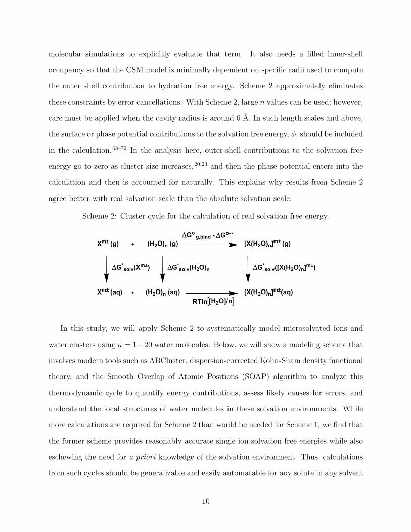
Scheme 2: Cluster cycle for the calculation of real solvation free energy.
In this study, we will apply Scheme 2 to systematically model microsolvated ions and
water clusters using n = 1�20 water molecules. Below, we will show a modeling scheme that
involves modern tools such as ABCluster, dispersion-corrected Kohn-Sham density functional
theory, and the Smooth Overlap of Atomic Positions (SOAP) algorithm to analyze this
thermodynamic cycle to quantify energy contributions, assess likely causes for errors, and
understand the local structures of water molecules in these solvation environments. While
more calculations are required for Scheme 2 than would be needed for Scheme 1, we find that
the former scheme provides reasonably accurate single ion solvation free energies while also
eschewing the need for a priori knowledge of the solvation environment. Thus, calculations
from such cycles should be generalizable and easily automatable for any solute in any solvent
10

environment.
3 Computational Methodology
We generated microsolvated solutes using the rigid molecular optimizer module of the AB-
Cluster program.53,54 We generated 1,000 low energy candidates using CHARMM force-
field parameters from MacKerell’s CGenFF website.73 Five low energy structures obtained
from the CHARMM forcefield optimization were then further optimized at the BP8674,75-
D3BJ76/def2-SVP77 or B3LYP78-D3BJ76/def2-SVP77 level of theory, as implemented in
ORCA79 using the RI-J or RIJCOSX approximations. Free energy contributions were cal-
culated using the ideal gas, rigid rotor, and harmonic oscillator approximations at the same
level of theory as the geometry optimizations. Finally, to assess the significance of higher
levels of theory, we calculated single point energies on fully optimized geometries at the
B3LYP78-D3BJ76/def2-TZVP77 and !B97X-D380/def2-TZVP77 levels of theory. Every en-
ergy reported in this manuscript is the Boltzmann-weighted average of the five low energy
structures identified with a global optimization code (ABCluster). The thermodynamic cycle
reported in Scheme 2 requires calculations on water clusters. To generate the water clusters,
we followed the same procedure outlined above using with TIP4P parameters for the water
molecules.81 Cluster geometries were then optimized at the same level of QM theory as the
solute-solvent clusters, as discussed above.
4 Results and Discussion
We first benchmarked low energy water clusters generated from ABCluster compared to
global minimum energy water clusters from the Cambridge Cluster Database that also used
the TIP4P forcefield.82 In all cases (n = 1, 2, 4, 8, 12, 16, 20), the energy di↵erences between
our structures and the reference structures from the database were all at most +1.2 kcal/mol
(Table S2). This agreement demonstrates that ABCluster is an e↵ective tool for identifying
11

low energy structures and that our water clusters are comparable to well-established and
globally optimized water cluster structures.
Next, we calculated solvation free energies of (H2O)n clusters using the thermodynamic
cycle outlined in Scheme S1 and compared it with solvation energy calculations using the
SMD solvation model. Table S3 shows solvation free energies for water clusters derived using
the thermodynamic cycle shown in Scheme S1, solvation free energies calculated directly
using a CSM, and the di↵erence between the two calculation schemes. For cases where
n = 2, 4, 8, the di↵erence in the two sets of solvation free energies is under 5 kcal/mol.
However, for larger clusters (n = 12, 16, 20), the di↵erence in free energies from these two
calculation schemes significantly increases by as much as 30 kcal/mol. This trend shows
that when relatively large clusters of water are solvated with a CSM, the model seems to
introduce significant errors that would then make them less reliable if used for calculations
with Scheme 2. The observation also in part justifies the use of QCT methods that use
Scheme 1 and relatively small cluster sizes. The lowest error arises with n = 4 because
it is the most probable size for water clusters, making the ln [pX(n)] term in Eq. 3 go
approximately to zero.
We then benchmarked calculated gas phase binding free energies of water molecules to
di↵erent ions against experimental data.83,84 Table S4 shows gas phase binding free energies
for one water molecule and di↵erent ions. For all the ions (Li+, Na+, K+, Cl�, Br�, F�),
calculations are in good agreement with the experimental data, and our errors are mostly
under 5 kcal/mol. We further compared the Na+ and K+ binding free energies with one wa-
ter molecule to other computational studies, and Table S4 shows that di↵erent calculations
agree reasonably well with experimental data.17,19 We also calculated binding free energies
involving four water molecules using Schemes 1 and 2, and compared them with both exper-
imental and other computational studies (Table S5). The reference experimental data used
for comparison add water molecules one by one to the system.83,84 Using Scheme 1, we get
very good agreement with the experimental values and our errors are under 5 kcal/mol for
12

all ions (Li+, Na+, K+, F�, Cl�, Br�). The data are also in relatively close agreement with
gas phase binding free energies calculated by Rempe and coworkers.24 However, when we
used Scheme 2 to calculate binding of ions to four water molecules, we obtained free energies
that di↵er from the prior work by 10 kcal/mol. This di↵erence is anticipated on the basis
that Scheme 2 applies to solvation reactions, not gas phase association reactions.
After benchmarking our calculations, we calculated hydration free energies using Eq. 6,
which relies on the cluster thermodynamic cycle as outlined in Scheme 2. We considered a
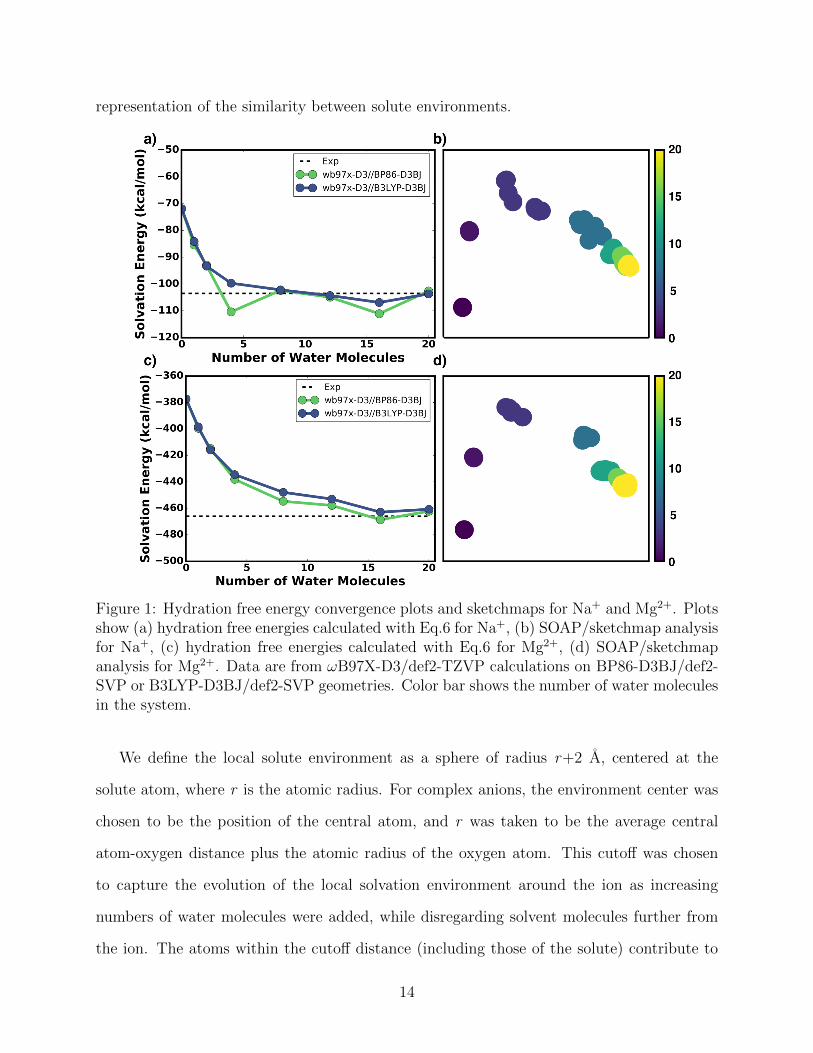
data set of ions having di↵erence sizes and charges of 2+, 1+, 1-, and 2-. Figures 1 and 2
show hydration free energies for Na+, Mg2+, Cl�, SO2�4 , and similar data are reported for all
ions and shown in Figures S1-S7. Table S6 shows hydration free energies for all the solutes,
and the percent error calculated by taking absolute hydration free energies from Marcus’s
study and adding the phase potential contribution taken from Lamoureux and Roux,50 using
Eq.1. In Figure 1a and 1c, for Na+ and Mg2+ cations, respectively, the hydration free energies
appear to converge steadily when we gradually increase the number of water molecules in the
system. In Figures 2a and 2c, for Cl� and SO2�4 anions, respectively, the same inference does
not hold. The anion hydration free energies are not particularly sensitive to water cluster
size, and hydration free energies begin to deviate more from experiment when using 16 and
20 water molecules. Thus, our initial hypothesis that adding more solvent molecules into
the system should generally improve the accuracy compared to experiment was mainly true
only for the cations we modeled.
We then hypothesized that di↵erent microsolvated ion clusters might have significantly
di↵erent solute structures, which result in di↵erent hydration free energies, as shown in
Figures 1 and 2. To test this idea, we studied geometric similarities in cluster sizes. We
used the Smooth Overlap for Atomic Positions (SOAP) kernel to quantify the similarity
between solute environments.56,57 For the high-dimensional pair-similarity data on solute
environments, we used “sketch-maps”, a non-linear dimensionality reduction technique.85,86
Sketch-maps allow us to obtain a two-dimensional map that provides a meaningful visual
13
representation of the similarity between solute environments.
Figure 1: Hydration free energy convergence plots and sketchmaps for Na+ and Mg2+. Plotsshow (a) hydration free energies calculated with Eq.6 for Na+, (b) SOAP/sketchmap analysisfor Na+, (c) hydration free energies calculated with Eq.6 for Mg2+, (d) SOAP/sketchmapanalysis for Mg2+. Data are from !B97X-D3/def2-TZVP calculations on BP86-D3BJ/def2-SVP or B3LYP-D3BJ/def2-SVP geometries. Color bar shows the number of water moleculesin the system.
We define the local solute environment as a sphere of radius r+2 A, centered at the
solute atom, where r is the atomic radius. For complex anions, the environment center was
chosen to be the position of the central atom, and r was taken to be the average central
atom-oxygen distance plus the atomic radius of the oxygen atom. This cuto↵ was chosen
to capture the evolution of the local solvation environment around the ion as increasing
numbers of water molecules were added, while disregarding solvent molecules further from
the ion. The atoms within the cuto↵ distance (including those of the solute) contribute to
14
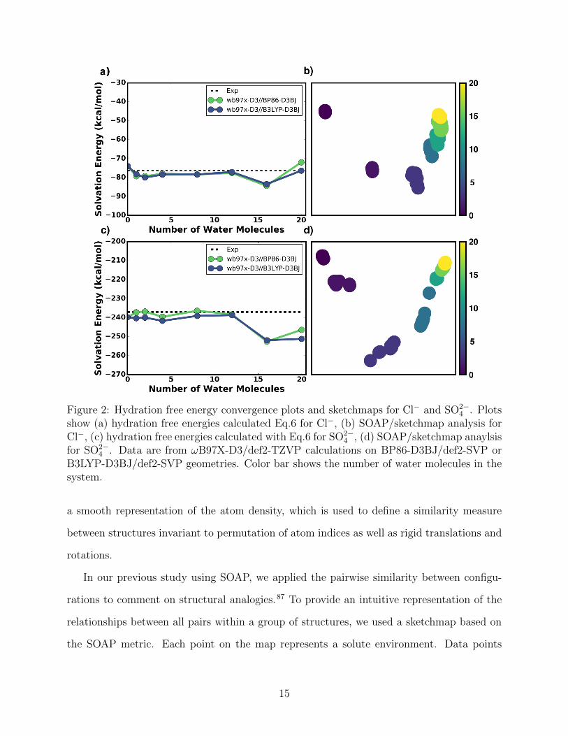
Figure 2: Hydration free energy convergence plots and sketchmaps for Cl� and SO2�4 . Plots
show (a) hydration free energies calculated Eq.6 for Cl�, (b) SOAP/sketchmap analysis forCl�, (c) hydration free energies calculated with Eq.6 for SO2�
4 , (d) SOAP/sketchmap anaylsisfor SO2�
4 . Data are from !B97X-D3/def2-TZVP calculations on BP86-D3BJ/def2-SVP orB3LYP-D3BJ/def2-SVP geometries. Color bar shows the number of water molecules in thesystem.
a smooth representation of the atom density, which is used to define a similarity measure
between structures invariant to permutation of atom indices as well as rigid translations and
rotations.
In our previous study using SOAP, we applied the pairwise similarity between configu-
rations to comment on structural analogies.87 To provide an intuitive representation of the
relationships between all pairs within a group of structures, we used a sketchmap based on
the SOAP metric. Each point on the map represents a solute environment. Data points
15

in close proximity indicate systems with high similarity in local solvent environments. The
sketchmap algorithm follows a non-linear optimization procedure where the discrepancy be-
tween pairwise Euclidean distances in low dimension and the kernel-induced metric is mini-
mized. A sigmoid function is applied to focus the optimization on the most relevant range
of distances, e.g. disregarding thermal fluctuations. The parameters of this filter are in the
format, sigma-a-b. In all cases, we used a=3 and b=8, while sigma values were adapted to
di↵erent systems following the heuristics described in Ref.88 In Figures 1 and 2, we used a
coloring scheme in which the color gets lighter when the size of the cluster increases. Yellow
dots represent the clusters that have 20 water molecules, and dark purple dots represent the
clusters with only one water molecule.
Figures 1b and 1d demonstrate that, for cations (Na+, Mg2+), convergence of the hy-
dration free energies goes hand-in-hand with the convergence of the structure of the first
solvation shell that evolves with increasingly larger numbers of water clusters. Given the
short-range cuto↵ for the SOAP descriptors, these results show that the convergence of the
hydration free energies for the cations correlates with the convergence of the local solvent
environment. However, this correspondence between structural and energetic convergence
is not observed for the anions (Cl�, SO2�4 ). The sketchmap for Cl� in Figure 2b shows
that local solvation environments start converging with n = 8, but there is a 10 kcal/mol
deviation in energy with clusters that involve 16 and 20 water molecules. A similar trend is
seen for the sketchmap for SO2�4 in Figure 2d. As with the cations, we see local solvation
structures converge starting with about n = 8, but the energies for 16 and 20 water clusters
are o↵ by 15 kcal/mol. This discrepancy suggests that the errors shown in Figure 2 with
16 and 20 water clusters likely arise from an imbalance in anharmonic e↵ects in Scheme 2
because the ion-water clusters have more anharmonicity than the water-water clusters.
To obtain a more detailed understanding of where the errors come from, we performed
MD simulations using the AMEOBA force field89 with the TINKER90 software package to
account for both chemical and thermal energy scales. We performed simulations for Na+
16
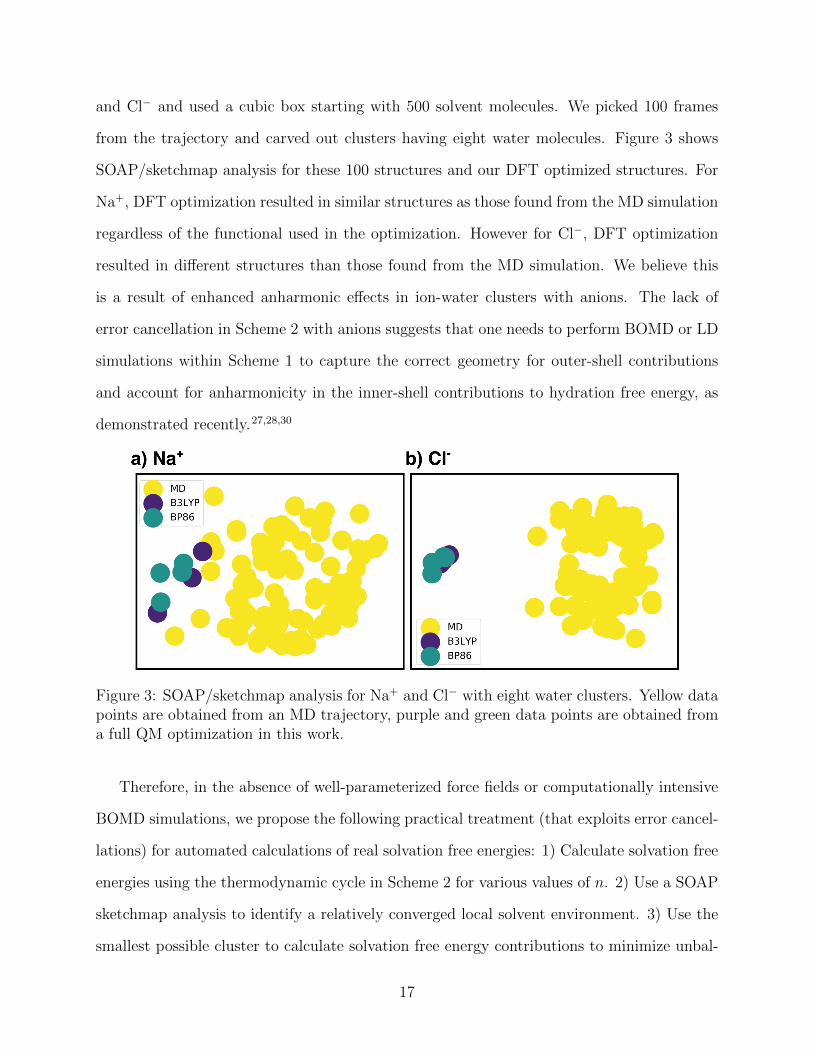
and Cl� and used a cubic box starting with 500 solvent molecules. We picked 100 frames
from the trajectory and carved out clusters having eight water molecules. Figure 3 shows
SOAP/sketchmap analysis for these 100 structures and our DFT optimized structures. For
Na+, DFT optimization resulted in similar structures as those found from the MD simulation
regardless of the functional used in the optimization. However for Cl�, DFT optimization
resulted in di↵erent structures than those found from the MD simulation. We believe this
is a result of enhanced anharmonic e↵ects in ion-water clusters with anions. The lack of
error cancellation in Scheme 2 with anions suggests that one needs to perform BOMD or LD
simulations within Scheme 1 to capture the correct geometry for outer-shell contributions
and account for anharmonicity in the inner-shell contributions to hydration free energy, as
demonstrated recently.27,28,30
Figure 3: SOAP/sketchmap analysis for Na+ and Cl� with eight water clusters. Yellow datapoints are obtained from an MD trajectory, purple and green data points are obtained froma full QM optimization in this work.
Therefore, in the absence of well-parameterized force fields or computationally intensive
BOMD simulations, we propose the following practical treatment (that exploits error cancel-
lations) for automated calculations of real solvation free energies: 1) Calculate solvation free
energies using the thermodynamic cycle in Scheme 2 for various values of n. 2) Use a SOAP
sketchmap analysis to identify a relatively converged local solvent environment. 3) Use the
smallest possible cluster to calculate solvation free energy contributions to minimize unbal-
17

anced errors that appear to arise from a CSM analysis of outer-shell contributions combined
with harmonic analysis of inner-shell contributions to solvation free energy.
5 Conclusion
We have demonstrated an automatable cluster-continuum (i.e., mixed implicit/explicit) mod-
eling approach to calculating solvation free energies of ions and small molecules that should
be applicable for other molecules not considered in this study. We elucidated Scheme 1
in practical applications limits analysis to small n and CSM models to account for outer-
shell contributions, and the results agree with absolute solvation free energies. In contrast,
Scheme 2 analyzes large n and large cluster sizes, where CSM models drop out and phase
potentials enter the calculation. We also showed how adding explicit solvent molecules
improves calculated solvation free energies by creating a more physical local solvation en-
vironment, but adding too many solvent molecules leads to significant errors in the CSM
combined with harmonic analysis of inner-shell. Overall, we show an approach to system-
atically investigate solvation environments alongside with converging solvation free energies.
The SOAP/sketchmap analysis can be combined with global optimization techniques such
as ABCluster to minimize the required prior knowledge needed to compute an accurate sol-
vation free energy using quantum chemistry. We expect this approach will be applicable to
other ions in water as well as ions in di↵erent solvents.
Acknowledgement
We acknowledge support from the R. K. Mellon Foundation and the National Science Foun-
dation (CBET-1653392 and CBET-1705592). We thank the University of Pittsburgh Center
for Research Computing for computing time and technical support.
18
Supporting Information Available
• Table S1: Comparison of di↵erent solvation scales in kcal/mol.
• Table S2: Comparison of calculated electronic energies of water clusters in kcal/mol.
• Scheme S1: Thermodynamic cycle for the formation of water clusters.
• Table S3: Energy contributions (in kcal/mol) used in solvation free energy calculations
of (H2O)n clusters at T = 298.15 K in kcal/mol.
• Table S4: Comparison of gas phase binding free energies for [X(H2O)] in kcal/mol.
• Table S5: Gas phase binding free energies of [X(H2O)4] in kcal/mol.
• Figure S1-S7: Hydration free energy convergence plots and sketchmaps for the remain-
ing solutes.
References
(1) Balbuena, P. B.; Johnston, K. P.; Rossky, P. J. Molecular dynamics simulation of
electrolyte solutions in ambient and supercritical water. 1. Ion solvation. J. Phys. Chem.
1996, 100, 2706–2715.
(2) Pickard IV, F. C.; Konig, G.; Simmonett, A. C.; Shao, Y.; Brooks, B. R. An e�cient
protocol for obtaining accurate hydration free energies using quantum chemistry and
reweighting from molecular dynamics simulations. Bioorg. Med. Chem. 2016, 24, 4988–
4997.
(3) Eggimann, B. L.; Siepmann, J. I. Size E↵ects on the Solvation of Anions at the Aqueous
Liquid- Vapor Interface. J. Phys. Chem. C 2008, 112, 210–218.
(4) Tomasi, J.; Persico, M. Molecular interactions in solution: an overview of methods
based on continuous distributions of the solvent. Chem. Rev. 1994, 94, 2027–2094.
19

(5) Miertus, S.; Scrocco, E.; Tomasi, J. Electrostatic interaction of a solute with a contin-
uum. A direct utilizaion of AB initio molecular potentials for the prevision of solvent
e↵ects. Chem. Phys. 1981, 55, 117–129.
(6) Cammi, R.; Tomasi, J. Remarks on the use of the apparent surface charges (ASC)
methods in solvation problems: Iterative versus matrix-inversion procedures and the
renormalization of the apparent charges. J. Comput. Chem. 1995, 16, 1449–1458.
(7) Klamt, A.; Schuurmann, G. COSMO: a new approach to dielectric screening in solvents
with explicit expressions for the screening energy and its gradient. J. Chem. Soc., Perkin
Trans. 2 1993, 799–805.
(8) Barone, V.; Cossi, M. Quantum calculation of molecular energies and energy gradients
in solution by a conductor solvent model. J. Phys. Chem. A 1998, 102, 1995–2001.
(9) Marenich, A. V.; Cramer, C. J.; Truhlar, D. G. Universal solvation model based on
solute electron density and on a continuum model of the solvent defined by the bulk
dielectric constant and atomic surface tensions. J. Phys. Chem. B 2009, 113, 6378–
6396.
(10) Plata, R. E.; Singleton, D. A. A case study of the mechanism of alcohol-mediated Morita
Baylis–Hillman reactions. The importance of experimental observations. J. Am. Chem.
Soc. 2015, 137, 3811–3826.
(11) Pratt, L. R.; Rempe, S. B. Quasi-chemical theory and implicit solvent models for sim-
ulations. AIP Conference Proceedings 1999, 492, 172–201.
(12) Asthagiri, D.; Dixit, P.; Merchant, S.; Paulaitis, M.; Pratt, L.; Rempe, S.; Varma, S.
Ion selectivity from local configurations of ligands in solutions and ion channels. Chem.
Phys. Lett. 2010, 485, 1 – 7.
20
(13) Rogers, D. M.; Jiao, D.; Pratt, L. R.; Rempe, S. B. Annual Reports in Computational
Chemistry ; Elsevier, 2012; Vol. 8; pp 71–127.
(14) Rempe, S. B.; Pratt, L. R.; Hummer, G.; Kress, J. D.; Martin, R. L.; Redondo, A. The
hydration number of Li+ in liquid water. J. Am. Chem. Soc. 2000, 122, 966–967.
(15) Rempe, S. B.; Pratt, L. R. The hydration number of Na+ in liquid water. Fluid Phase
Equilib. 2001, 183, 121–132.
(16) Rempe, S. B.; Asthagiri, D.; Pratt, L. R. Inner shell definition and absolute hydration
free energy of K+(aq) on the basis of quasi-chemical theory and ab initio molecular
dynamics. Phys. Chem. Chem. Phys. 2004, 6, 1966–1969.
(17) Varma, S.; Rempe, S. B. Structural transitions in ion coordination driven by changes
in competition for ligand binding. J. Am. Chem. Soc. 2008, 130, 15405–15419.
(18) Sabo, D.; Jiao, D.; Varma, S.; Pratt, L.; Rempe, S. Case study of Rb+(aq), quasi-
chemical theory of ion hydration, and the no split occupancies rule. Annual Reports
Section C (Physical Chemistry) 2013, 109, 266–278.
(19) Soniat, M.; Rogers, D. M.; Rempe, S. B. Dispersion-and exchange-corrected density
functional theory for sodium ion hydration. J. Chem. Theory Comput. 2015, 11, 2958–
2967.
(20) Chaudhari, M. I.; Soniat, M.; Rempe, S. B. Octa-coordination and the aqueous Ba2+
ion. J. Phys. Chem. B 2015, 119, 8746–8753.
(21) Chaudhari, M. I.; Rempe, S. B. Strontium and barium in aqueous solution and a
potassium channel binding site. J. Chem. Phys. 2018, 148, 222831.
(22) Chaudhari, M. I.; Pratt, L. R.; Rempe, S. B. Utility of chemical computations in
predicting solution free energies of metal ions. Mol. Simulat. 2018, 44, 110–116.
21
(23) Biomolecular Hydration Mimicry in Ion Permeation through Membrane Channels. Acc.
Chem. Res. 2019,
(24) Asthagiri, D.; Pratt, L. R.; Paulaitis, M. E.; Rempe, S. B. Hydration structure and free
energy of biomolecularly specific aqueous dications, including Zn2+ and first transition
row metals. J. Am. Chem. Soc. 2004, 126, 1285–1289.
(25) Jiao, D.; Leung, K.; Rempe, S. B.; Neno↵, T. M. First principles calculations of atomic
nickel redox potentials and dimerization free energies: A study of metal nanoparticle
growth. J. Chem. Theory Comput. 2010, 7, 485–495.
(26) Chaudhari, M. I.; Rempe, S. B.; Pratt, L. R. Quasi-chemical theory of F�(aq): The
“no split occupancies rule” revisited. J. Chem. Phys. 2017, 147, 161728.
(27) Muralidharan, A.; Pratt, L. R.; Chaudhari, M. I.; Rempe, S. B. Quasi-chemical theory
with cluster sampling from ab initio molecular dynamics: Fluoride (F�) anion hydra-
tion. J. Phys. Chem. A 2018, 122, 9806–9812.
(28) Muralidharan, A.; Pratt, L. R.; Chaudhari, M. I.; Rempe, S. B. Quasi-Chemical Theory
for Anion Hydration and Specific Ion E↵ects: Cl�(aq) vs. F�(aq). Chem. Phys. Lett.
2019,
(29) Ashbaugh, H. S.; Asthagiri, D.; Pratt, L. R.; Rempe, S. B. Hydration of krypton and
consideration of clathrate models of hydrophobic e↵ects from the perspective of quasi-
chemical theory. Biophys. Chem. 2003, 105, 323–338.
(30) Sabo, D.; Varma, S.; Martin, M. G.; Rempe, S. B. Studies of the thermodynamic
properties of hydrogen gas in bulk water. The Journal of Physical Chemistry B 2008,
112, 867–876.
(31) Clawson, J. S.; Cygan, R. T.; Alam, T. M.; Leung, K.; Rempe, S. B. Ab initio study of
hydrogen storage in water clathrates. J. Comput. Theor. Nanosci. 2010, 7, 2602–2606.
22

(32) Jiao, D.; Rempe, S. B. CO2 solvation free energy using quasi-chemical theory. J. Chem.
Phys. 2011, 134, 224506.
(33) Chaudhari, M. I.; Nair, J. R.; Pratt, L. R.; Soto, F. A.; Balbuena, P. B.; Rempe, S. B.
Scaling atomic partial charges of carbonate solvents for lithium ion solvation and dif-
fusion. J. Chem. Theory Comput. 2016, 12, 5709–5718.
(34) Varma, S.; Rempe, S. B. Tuning ion coordination architectures to enable selective
partitioning. Biophys. J. 2007, 93, 1093 – 1099.
(35) Varma, S.; Sabo, D.; Rempe, S. B. K+/Na+ Selectivity in K Channels and Valinomycin:
Over-coordination Versus Cavity-size constraints. J. Mol. Biol. 2008, 376, 13 – 22.
(36) Varma, S.; Rogers, D. M.; Pratt, L. R.; Rempe, S. B. Design principles for K+ selectivity
in membrane transport. J. Gen. Physiol. 2011, 137, 479–488.
(37) Rogers, D. M.; Rempe, S. B. Probing the thermodynamics of competitive ion binding
using minimum energy structures. J. Phys. Chem. B 2011, 115, 9116–9129.
(38) Jiao, D.; Rempe, S. B. Combined Density Functional Theory (DFT) and Continuum
Calculations of pKa in Carbonic Anhydrase. Biochem. 2012, 51, 5979–5989.
(39) Rossi, M.; Tkatchenko, A.; Rempe, S. B.; Varma, S. Role of methyl-induced polarization
in ion binding. Proc. Natl. Acad. Sci. U.S.A. 2013, 110, 12978–12983.
(40) Stevens, M. J.; Rempe, S. L. Ion-specific e↵ects in carboxylate binding sites. J. Phys.
Chem. B 2016, 120, 12519–12530.
(41) Mennucci, B.; Martınez, J. M. How to model solvation of peptides? Insights from
a quantum-mechanical and molecular dynamics study of N-methylacetamide. 1. Ge-
ometries, infrared, and ultraviolet spectra in water. J. Phys. Chem. B 2005, 109,
9818–9829.
23

(42) Fennell, C. J.; Dill, K. A. Physical modeling of aqueous solvation. J. Stat. Phys. 2011,
145, 209–226.
(43) Pratt, L. R. Contact potentials of solution interfaces: phase equilibrium and interfacial
electric fields. J. Phys. Chem. 1992, 96, 25–33.
(44) Leung, K.; Rempe, S. B.; von Lilienfeld, O. A. Ab initio molecular dynamics calculations
of ion hydration free energies. J. Chem. Phys. 2009, 130, 204507.
(45) Lyklema, J. Interfacial Potentials: Measuring the Immeasurable? Substantia 2017, 1 .
(46) Doyle, C. C.; Shi, Y.; Beck, T. L. The Importance of the Water Molecular Quadrupole
for Estimating Interfacial Potential Shifts Acting on Ions Near the Liquid-Vapor Inter-
face. J. Phys. Chem. B 2019,
(47) Marcus, Y. Thermodynamics of solvation of ions. Part 5.Gibbs free energy of hydration
at 298.15 K. J. Chem. Soc., Faraday Trans. 1991, 87, 2995–2999.
(48) Marcus, Y. The thermodynamics of solvation of ions. Part 4.Application of the
tetraphenylarsonium tetraphenylborate (TATB) extrathermodynamic assumption to
the hydration of ions and to properties of hydrated ions. J. Chem. Soc., Faraday Trans.
1 1987, 83, 2985–2992.
(49) Tissandier, M. D.; Cowen, K. A.; Feng, W. Y.; Gundlach, E.; Cohen, M. H.;
Earhart, A. D.; Coe, J. V.; Tuttle, T. R. The proton’s absolute aqueous enthalpy
and Gibbs free energy of solvation from cluster-ion solvation data. J. Phys. Chem. A
1998, 102, 7787–7794.
(50) Lamoureux, G.; Roux, B. Absolute hydration free energy scale for alkali and halide ions
established from simulations with a polarizable force field. J. Phys. Chem. B 2006, 110,
3308–3322.
24
(51) Bryantsev, V. S.; Diallo, M. S.; Goddard III, W. A. Computational study of copper
(II) complexation and hydrolysis in aqueous solutions using mixed cluster/continuum
models. J. Phys. Chem. A 2009, 113, 9559–9567.
(52) Wu, W.; Kie↵er, J. New Hybrid Method for the Calculation of the Solvation Free
Energy of Small Molecules in Aqueous Solutions. J. Chem. Theory Comput. 2018, 15,
371–381.
(53) Zhang, J.; Dolg, M. ABCluster: the artificial bee colony algorithm for cluster global
optimization. Phys. Chem. Chem. Phys. 2015, 17, 24173–24181.
(54) Zhang, J.; Dolg, M. Global optimization of clusters of rigid molecules using the artificial
bee colony algorithm. Phys. Chem. Chem. Phys. 2016, 18, 3003–3010.
(55) Bryantsev, V. S.; Diallo, M. S.; Goddard Iii, W. A. Calculation of solvation free energies
of charged solutes using mixed cluster/continuum models. J. Phys. Chem. B 2008, 112,
9709–9719.
(56) Bartok, A. P.; Kondor, R.; Csanyi, G. On representing chemical environments. Phys.
Rev. B 2013, 87, 184115.
(57) De, S.; Bartok, A. P.; Csanyi, G.; Ceriotti, M. Comparing molecules and solids across
structural and alchemical space. Phys. Chem. Chem. Phys. 2016, 18, 13754–13769.
(58) Pliego, J. R.; Riveros, J. M. The cluster- continuum model for the calculation of the
solvation free energy of ionic species. J. Phys. Chem. A 2001, 105, 7241–7247.
(59) Zhan, C.-G.; Dixon, D. A. Absolute hydration free energy of the proton from first-
principles electronic structure calculations. J. Phys. Chem. A 2001, 105, 11534–11540.
(60) Kelly, C. P.; Cramer, C. J.; Truhlar, D. G. Aqueous solvation free energies of ions and
ion- water clusters based on an accurate value for the absolute aqueous solvation free
energy of the proton. J. Phys. Chem. B 2006, 110, 16066–16081.
25
(61) Riccardi, D.; Guo, H.-B.; Parks, J. M.; Gu, B.; Liang, L.; Smith, J. C. Cluster-
continuum calculations of hydration free energies of anions and group 12 divalent
cations. J. Chem. Theory Comput. 2012, 9, 555–569.
(62) Beck, T. L.; Paulaitis, M. E.; Pratt, L. R. The Potential Distribution Theorem and
Models of Molecular Solutions ; Cambridge University Press, 2006.
(63) Varma, S.; Rempe, S. B. Coordination numbers of alkali metal ions in aqueous solutions.
Biophy. Chem. 2006, 124, 192 – 199, Ion Hydration Special Issue.
(64) Sabo, D.; Rempe, S.; Greathouse, J.; Martin, M. Molecular studies of the structural
properties of hydrogen gas in bulk water. Mol. Simulat. 2006, 32, 269–278.
(65) Mason, P. E.; Ansell, S.; Neilson, G.; Rempe, S. B. Neutron Scattering Studies of the
Hydration Structure of Li+. J. Phys. Chem. B 2015, 119, 2003–2009.
(66) Caminiti, R.; Licheri, G.; Piccaluga, G.; Pinna, G. X-ray Di↵raction Study of MgCl2
Aqueous Solutions. J. Appl. Cryst. 1979, 12, 34–38.
(67) da Silva, E. F.; Svendsen, H. F.; Merz, K. M. Explicitly representing the solvation shell
in continuum solvent calculations. J. Phys. Chem. A 2009, 113, 6404–6409.
(68) Pollard, T.; Beck, T. L. Quasichemical analysis of the cluster-pair approximation for
the thermodynamics of proton hydration. J. Chem. Phys. 2014, 140, 224507.
(69) Pollard, T. P.; Beck, T. L. The thermodynamics of proton hydration and the electro-
chemical surface potential of water. J. Chem. Phys. 2014, 141, 18C512.
(70) Pollard, T. P.; Beck, T. L. Re-examining the tetraphenyl-arsonium/tetraphenyl-borate
(TATB) hypothesis for single-ion solvation free energies. J. Chem. Phys. 2018, 148,
222830.
(71) Shi, Y.; Beck, T. L. Length scales and interfacial potentials in ion hydration. J. Chem.
Phys. 2013, 139, 044504.
26

(72) Beck, T. L. The influence of water interfacial potentials on ion hydration in bulk water
and near interfaces. Chem. Phys. Lett 2013, 561, 1–13.
(73) Vanommeslaeghe, K.; Hatcher, E.; Acharya, C.; Kundu, S.; Zhong, S.; Shim, J.; Dar-
ian, E.; Guvench, O.; Lopes, P.; Vorobyov, I.; Mackerell, A. CHARMM general force
field: A force field for drug-like molecules compatible with the CHARMM all-atom
additive biological force fields. J. Comput. Chem. 2010, 31, 671–690.
(74) Perdew, J. P. Density-functional approximation for the correlation energy of the inho-
mogeneous electron gas. Phys. Rev. B 1986, 33, 8822.
(75) Becke, A. D. Density-functional exchange-energy approximation with correct asymp-
totic behavior. Phys. Rev. A 1988, 38, 3098.
(76) Grimme, S.; Ehrlich, S.; Goerigk, L. E↵ect of the damping function in dispersion cor-
rected density functional theory. J. Comput. Chem. 2011, 32, 1456–1465.
(77) Weigend, F.; Ahlrichs, R. Balanced basis sets of split valence, triple zeta valence and
quadruple zeta valence quality for H to Rn: Design and assessment of accuracy. Phys.
Chem. Chem. Phys. 2005, 7, 3297–3305.
(78) Becke, A. D. Density-functional thermochemistry. III. The role of exact exchange. J.
Chem. Phys. 1993, 98, 5648–5652.
(79) Neese, F. The ORCA program system.Wiley Interdiscip. Rev. Comput. Mol. Sci. 2012,
2, 73–78.
(80) Chai, J.-D.; Head-Gordon, M. Long-range corrected hybrid density functionals with
damped atom–atom dispersion corrections. Phys. Chem. Chem. Phys. 2008, 10, 6615–
6620.
(81) Abascal, J. L.; Vega, C. A general purpose model for the condensed phases of water:
TIP4P/2005. J. Chem. Phys. 2005, 123, 234505.
27
(82) Wales, D. J.; Hodges, M. P. Global minima of water clusters (H2O)n, n 21, described
by an empirical potential. Chem. Phys. Lett 1998, 286, 65–72.
(83) Arshadi, M.; Yamdagni, R.; Kebarle, P. Hydration of the halide negative ions in the gas
phase. II. Comparison of hydration energies for the alkali positive and halide negative
ions. J. Phys. Chem. 1970, 74, 1475–1482.
(84) Dzidic, I.; Kebarle, P. Hydration of the alkali ions in the gas phase. Enthalpies and
entropies of reactions M+(H2O)n�1+ H2O = M+ (H2O)n. J. Phys. Chem. 1970, 74,
1466–1474.
(85) Ceriotti, M.; Tribello, G. A.; Parrinello, M. Simplifying the representation of complex
free-energy landscapes using sketch-map. Proc. Natl. Acad. Sci. U.S.A. 2011, 108,
13023–13028.
(86) Ceriotti, M.; Tribello, G. A.; Parrinello, M. Demonstrating the transferability and the
descriptive power of sketch-map. J. Chem. Theory Comput. 2013, 9, 1521–1532.
(87) Basdogan, Y.; Keith, J. A. A paramedic treatment for modeling explicitly solvated
chemical reaction mechanisms. Chem. Sci. 2018, 9, 5341–5346.
(88) De, S.; Musil, F.; Ingram, T.; Baldauf, C.; Ceriotti, M. Mapping and classifying
molecules from a high-throughput structural database. J. Cheminform. 2017, 9, 6.
(89) Ponder, J. W.; Wu, C.; Ren, P.; Pande, V. S.; Chodera, J. D.; Schnieders, M. J.;
Haque, I.; Mobley, D. L.; Lambrecht, D. S.; DiStasio Jr, R. A.; Head-Gordon, M.
Current status of the AMOEBA polarizable force field. J. Phys. Chem. B 2010, 114,
2549–2564.
(90) Ponder, J. W. TINKER: Software tools for molecular design. 2004,
28
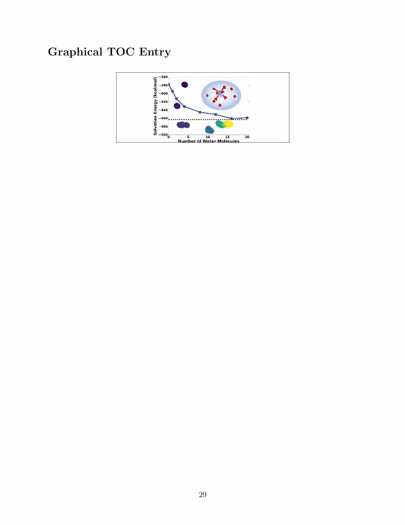
Graphical TOC Entry
29

Machine Learning Guided Approach for
Studying Solvation Environments
Yasemin Basdogan,†
Mitchell C. Groenenboom,†
Ethan Henderson,†
Sandip De,‡
Susan Rempe,¶
and John A. Keith⇤,†
†Department of Chemical and Petroleum Engineering Swanson School of Engineering,
University of Pittsburgh, Pittsburgh, USA
‡Laboratory of Computational Science and Modelling, Institute of Materials, École
Polytechnique Fédérale de Lausanne, Lausanne, Switzerland
¶Department of Nanobiology, Sandia National Laboratories, Albuquerque, USA
E-mail: [email protected]
Table S1: Comparison of different solvation scales in kcal/mol.
Ion TATB [a] CPB [b] DifferenceLi+ �113.5 �126.5 �13.0Na+ �87.2 �101.3 �14.1K+ �70.5 �84.1 �13.6F� �111.1 �102.5 8.6Cl� �81.3 �72.7 8.6Br� �75.3 �66.3 9.0[a] Data taken from Ref.1[b] Cluster pair-base data (CPB). Data taken from taken from Ref.2
S1

Table S2: Comparison of calculated electronic energies of water clusters in kcal/mol. [a]
n Globally optimized clusters [b] ABCluster clusters [c] Difference2 -95924.5 -95924.1 0.44 -191852.8 -191852.1 0.78 -383710.1 -383708.9 1.212 -575564.3 -575564.0 0.316 -767420.3 -767420.2 0.120 -959279.6 -959279.0 0.6
[a] Single point electronic energies calculated using !B97X-D3/def2-TZVP.[b] Geometries taken from Ref.3 and then reoptimized using BP86-D3BJ/def2-SVP.[c] Geometries obtained using the procedure stated in the main text.
Scheme 1: Thermodynamic cycle for the formation of water clusters.
S2
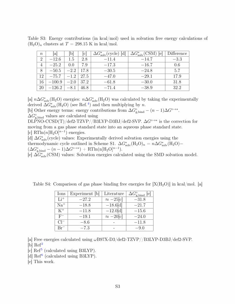
Table S3: Energy contributions (in kcal/mol) used in solvation free energy calculations of(H2O)n clusters at T = 298.15 K in kcal/mol.
n [a] [b] [c] �G⇤solv(cycle) [d] �G⇤
solv(CSM) [e] Difference2 �12.6 1.5 2.8 �11.4 �14.7 �3.34 �25.2 0.0 7.9 �17.3 �16.7 0.68 �50.5 �2.2 17.8 �30.5 �24.8 5.712 �75.7 �1.2 27.5 �47.0 �29.1 17.916 �100.9 �2.0 37.2 �61.8 �30.0 31.820 �126.2 �8.1 46.8 �71.4 �38.9 32.2
[a] n�G⇤solv(H2O) energies: n�G⇤
solv(H2O) was calculated by taking the experimentallyderived �G⇤
solv(H2O) (see Ref.4) and then multiplying by n.[b] Other energy terms: energy contributions from �G�
g,bind � (n� 1)�G�!⇤.�G�
g,bind values are calculated usingDLPNO-CCSD(T)/def2-TZVP//B3LYP-D3BJ/def2-SVP. �G�!⇤ is the correction formoving from a gas phase standard state into an aqueous phase standard state.[c] RTln(n[H2O]n�1) energies.[d] �G⇤
solv(cycle) values: Experimentally derived solvation energies using thethermodynamic cycle outlined in Scheme S1. �G⇤
solv(H2O)n = n�G⇤solv(H2O)�
(�G�g,bind � (n� 1)�G�!⇤) + RTln(n[H2O]n�1).
[e] �G⇤solv(CSM) values: Solvation energies calculated using the SMD solvation model.
Table S4: Comparison of gas phase binding free energies for [X(H2O)] in kcal/mol. [a]
Ions Experiment [b] Literature �G�g,bind [e]
Li+ �27.2 ⇡ �25[c] �31.8Na+ �18.8 �18.6[d] �21.7K+ �11.8 �12.0[d] �15.6F� �19.1 ⇡ �20[c] �24.0Cl� �8.6 - �11.8Br� �7.3 - �9.0
[a] Free energies calculated using !B97X-D3/def2-TZVP//B3LYP-D3BJ/def2-SVP.[b] Ref2
[c] Ref5 (calculated using B3LYP).[d] Ref6 (calculated using B3LYP).[e] This work.
S3
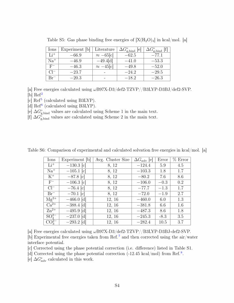
Table S5: Gas phase binding free energies of [X(H2O)4] in kcal/mol. [a]
Ions Experiment [b] Literature �G�g,bind [e] �G�
g,bind [f]Li+ �66.9 ⇡ �65[c] �62.5 �77.1Na+ �46.9 �49.4[d] �41.0 �53.3F� �46.3 ⇡ �45[c] �49.8 �52.0Cl� �23.7 - �24.2 �29.5Br� �20.3 - �18.2 �26.3
[a] Free energies calculated using !B97X-D3/def2-TZVP//B3LYP-D3BJ/def2-SVP.[b] Ref2
[c] Ref5 (calculated using B3LYP).[d] Ref6 (calculated using B3LYP).[e] �G�
g,bind values are calculated using Scheme 1 in the main text.[f] �G�
g,bind values are calculated using Scheme 2 in the main text.
Table S6: Comparison of experimental and calculated solvation free energies in kcal/mol. [a]
Ions Experiment [b] Avg. Cluster Size �Gsolv [e] Error % ErrorLi+ �130.3 [c] 8, 12 �124.4 5.9 4.5Na+ �105.1 [c] 8, 12 �103.3 1.8 1.7K+ �87.8 [c] 8, 12 �80.2 7.6 8.6F� �106.3 [c] 8, 12 �106.0 �0.3 0.2Cl� �76.4 [c] 8, 12 �77.7 �1.3 1.7Br� �70.1 [c] 8, 12 �72.0 �1.9 2.7
Mg2+ �466.0 [d] 12, 16 �460.0 6.0 1.3Ca2+ �388.4 [d] 12, 16 �381.8 6.6 1.6Zn2+ �495.9 [d] 12, 16 �487.3 8.6 1.8SO2�
4 �237.0 [d] 12, 16 �245.3 -8.3 3.5CO2�
3 �293.2 [d] 12, 16 �282.4 10.5 3.7
[a] Free energies calculated using !B97X-D3/def2-TZVP//B3LYP-D3BJ-def2-SVP.[b] Experimental free energies taken from Ref.7 and then corrected using the air/waterinterface potential.[c] Corrected using the phase potential correction (i.e. difference) listed in Table S1.[d] Corrected using the phase potential correction (-12.45 kcal/mol) from Ref.8.[e] �G⇤
solv calculated in this work.
S4

Figure S1: Hydration free energy convergence plot and sketchmap for Li+. Figure S1a showshydration free energy convergence plot calculated with Eq.6 in the main text for Li+. FigureS1b is the SOAP/sketchmap analysis for Li+.
Figure S2: Hydration free energy convergence plot and sketchmap for K+. Figure S2a showshydration free energy convergence plot calculated with Eq.6 in the main text for K+. FigureS2b is the SOAP/sketchmap analysis for K+.
S5

Figure S3: Hydration free energy convergence plot and sketchmap for F�. Figure S3a showshydration free energy convergence plot calculated with Eq.6 in the main text for F�. FigureS3b is the SOAP/sketchmap analysis for F�.
Figure S4: Hydration free energy convergence plot and sketchmap for Br�. Figure S4a showshydration free energy convergence plot calculated with Eq.6 in the main text for Br�. FigureS4b is the SOAP/sketchmap analysis for Br�.
S6

Figure S5: Hydration free energy convergence plot and sketchmap for Ca2+. Figure S5ashows hydration free energy convergence plot calculated with Eq.6 in the main text forCa2+. Figure S5b is the SOAP/sketchmap analysis for Ca2+.
Figure S6: Hydration free energy convergence plot and sketchmap for Zn2+. Figure S6ashows hydration free energy convergence plot calculated with Eq.6 in the main text forZn2+. Figure S6b is the SOAP/sketchmap analysis for Zn2+.
S7
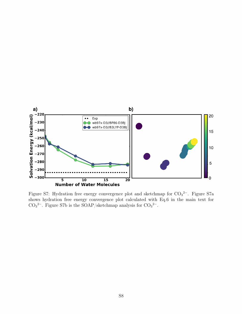
Figure S7: Hydration free energy convergence plot and sketchmap for CO32�. Figure S7a
shows hydration free energy convergence plot calculated with Eq.6 in the main text forCO3
2�. Figure S7b is the SOAP/sketchmap analysis for CO32�.
S8

References
(1) Marcus, Y. The thermodynamics of solvation of ions. Part 4.—Application of the
tetraphenylarsonium tetraphenylborate (TATB) extrathermodynamic assumption to the
hydration of ions and to properties of hydrated ions. J. Chem. Soc., Faraday Trans. 1
1987, 83, 2985–2992.
(2) Tissandier, M. D.; Cowen, K. A.; Feng, W. Y.; Gundlach, E.; Cohen, M. H.;
Earhart, A. D.; Coe, J. V.; Tuttle, T. R. The proton’s absolute aqueous enthalpy and
Gibbs free energy of solvation from cluster-ion solvation data. J. Phys. Chem. A 1998,
102, 7787–7794.
(3) Wales, D. J.; Hodges, M. P. Global minima of water clusters (H2O)n, n 21, described
by an empirical potential. Chem. Phys. Lett 1998, 286, 65–72.
(4) Keith, J. A.; Carter, E. A. Quantum Chemical Benchmarking, Validation, and Prediction
of Acidity Constants for Substituted Pyridinium Ions and Pyridinyl Radicals. Journal
of chemical theory and computation 2012, 8, 3187–3206.
(5) Muralidharan, A.; Pratt, L. R.; Chaudhari, M. I.; Rempe, S. B. Quasi-chemical theory
with cluster sampling from ab initio molecular dynamics: Fluoride (F�) anion hydration.
J. Phys. Chem. A 2018, 122, 9806–9812.
(6) Varma, S.; Rempe, S. B. Structural transitions in ion coordination driven by changes in
competition for ligand binding. J. Am. Chem. Soc. 2008, 130, 15405–15419.
(7) Marcus, Y. Thermodynamics of solvation of ions. Part 5.—Gibbs free energy of hydration
at 298.15 K. J. Chem. Soc., Faraday Trans. 1991, 87, 2995–2999.
(8) Lamoureux, G.; Roux, B. Absolute hydration free energy scale for alkali and halide ions
established from simulations with a polarizable force field. J. Phys. Chem. B 2006, 110,
3308–3322.
S9

download fileview on ChemRxivSolvation_ChemRxiv.pdf (8.41 MiB)