Machine Learning for Auxiliary Sources

Daniele Casati 1

AbstractWe rewrite the numerical ansatz of the Methodof Auxiliary Sources (MAS), typically used incomputational electromagnetics, as a neural net-work, i.e. as a composed function of linear andactivation layers. MAS is a numerical methodfor Partial Differential Equations (PDEs) that em-ploys point sources, which are also exact solutionsof the considered PDE, as radial basis functions tomatch a given boundary condition. In the frame-work of neural networks we rely on optimizationalgorithms such as Adam to train MAS and findboth its optimal coefficients and positions of thecentral singularities of the sources. In this workwe also show that the MAS ansatz trained as aneural network can be used, in the case of anunknown function with a central singularity, todetect the position of such singularity.

1. IntroductionComputational electromagnetics studies how to numericallysolve Maxwell’s boundary value problems for engineeringand scientific applications. An example is the simulation ofplasmonic nanoparticles, which can exhibit an interestingbehavior (such as scattering) with electromagnetic radiationat a wavelength far larger than the particle size, dependingon, e.g., the particle geometry (Koch et al., 2018). Thisphenomenon is relevant for many applications, such as solarcells or cancer treatment.

For this kind of problems, several numerical methods havebeen developed based on a partition of the geometric do-main: for example, the finite-difference time-domain method(Yee, 1966), using a regular grid, or the Finite ElementMethod (FEM) for frequency-domain Maxwell’s equations(Hiptmair, 2002), using an unstructured mesh typically

1Integrated Systems Laboratory, D-ITET, ETHZurich, Switzerland. Correspondence to: Daniele Casati<dcasati@iis.ee.ethz.ch>.

Copyright 2021 by the author.0Abbreviations. FEM: Finite Element Method. PDE: Partial

Differential Equation. MMP: Multiple Multipole Program. MAS:Method of Auxiliary Sources.

made of triangles (2D) or tetrahedra (3D). These approachesemploy basis functions locally supported on the entities ofthe partition and therefore lead to large, sparse linear sys-tems to solve.

Conversely, another line of research in computational elec-tromagnetics involves methods that do not need a mesh,as they make use of global basis functions (nonzero every-where) that are exact solutions of the Partial DifferentialEquation (PDE) of interest. Given their nature, these ba-sis functions do not need to be as many as the elements ofFEM to achieve a good approximation, but, as we will seein a moment, require additional care. The numerical solu-tion here is obtained by matching on a hypersurface eithera boundary condition or interface conditions with anotherdomain, discretized by 1) different basis functions, as thePDE may be different there, or 2) an entirely other method(Casati & Hiptmair, 2019).

More details on these so-called Trefftz methods (Hiptmairet al., 2016) are given in the next section. Here it sufficesto say that a common choice of Trefftz basis functions arepoint sources, i.e. exact solutions that exhibit a central sin-gularity. The centers of these singularities are placed in thecomplement of the respective domain of approximation, sothat they are ignored by the computations.

Furthermore, one would like to position these singularitiesin a way that the unknown function is well approximated bya linear combination of the sources. This holds true evenif it can be proven that Trefftz methods enjoy exponentialconvergence when the unknown function has an analyticcontinuation beyond its approximation domain (Casati &Hiptmair, 2019): as an example, please refer to the results intable 1 below. In a way, the goal here is similar to choosing ahigh-quality unstructured mesh for FEM (Brenner & Scott,2008) before assemblying and solving the related linearsystem.

To find this “optimal” positioning of the sources, the state-of-the-art is based on elaborate heuristic rules developedover the years to support the user’s manual positioning, es-pecially in the context of computational electromagnetics,where one Trefftz method is the Multiple Multipole Pro-gram1 (MMP) (Hafner, 1999). These heuristic rules are

1MMP is implemented by the open-source academic softwareOpenMaXwell (Hafner, 1999), whose first development dates

arX

iv:2

102.

0285

5v1

[ph

ysic

s.co

mp-

ph]

4 F

eb 2

021

Machine Learning for Auxiliary Sources

Table 1. Relative L2(Ω)-error of 3 point sources to approximate(1) for 10 different centers σ before and after the optimization(5 · 105 epochs).

INITIALPOSITIONS

AFTERALGORITHM

51.19% 1.32%32.07% 1.09%44.83% 1.01%10.70% 0.85%78.28% 0.94%15.37% 2.40%28.23% 1.26%32.15% 3.63%10.11% 1.29%

based on the curvature radius (Moreno et al.) or on anunstructured surface mesh (Koch et al., 2018) of the hyper-surface where the boundary condition needs to be imposed.Another line of research made use of genetic algorithms(Heretakis et al., 2005).

Here we propose an approach based on an optimization al-gorithm usually employed to train neural networks. As anumerical example for validation, let us consider for sim-plicity a Poisson’s problem in a 2D bounded domain Ω – incomputational electromagnetics it can model, e.g., a vec-tor magnetic potential orthogonal to the 2D plane – with amanufactured solution of the type

ρ−1xσ sin(θxσ), (1)

expressed in polar coordinates (r ∈ [0,∞), θ ∈ [0, 2π)) ofxσ := x− σ, with x,σ ∈ R2 position vectors in Cartesiancoordinates. Specifically, the center σ is taken in R2 \ Ω.

Let us then approximate2 this problem with 3 point sources,randomly placed in R2 \Ω not too far from the hypersurfaceΓ := ∂Ω, and obtain their coefficients in a least-squaressense by matching the values of (1) on selected points of Γ.

Table 1 presents the corresponding L2(Ω)-error (given abounded Ω) of this ansatz with respect to (1), considering10 different random centers σ not too far from Γ. The firstcolumn lists the relative errors (with respect to the L2(Ω)-norm of (1)) for this random placement of the sources, whichare as high as 78.28%. Conversely, as shown by the errorsin the second column, placing the sources with the optimiza-tion algorithm proposed in this work allows to achieve abetter approximation with the same ansatz.

back to 1980 and which provides a graphical interface for theuser to manually position the sources and check the correspondingnumerical solution.

2More details on the approximation ansatz are given in Sec-tion 2, on the experimental setup in Section 4.

1.1. Summary and Structure

Compared to the state-of-the-art of Trefftz methods, byusing the approach proposed in this paper we claim

• a higher accuracy, as shown by the results of table 1,which can also improve the more epochs are consideredfor the optimization,

• at a low additional runtime, given the efficient imple-mentations of the optimization algorithms for neuralnetworks: it takes a matter of seconds for the 5 · 105

epochs of table 1.

• This is also supported by the fact that the centers ofthe sources form a limited quantity of additional de-grees of freedom for the optimization algorithm (ontop of the coefficients of the sources). In fact, theirnumber is not high (typically of an order of magnitudeof 2) because of the exponential convergence of Trefftzmethods. This allows to handle large system sizes forreal-world engineering applications without particularrestrictions.

The work is organized as follows: after this introduction,the fundamentals of Trefftz methods, specifically of MMP,are presented in Section 2. Next, details on how to use theoptimization algorithms of neural networks for MMP aregiven in Section 3. This approach is then supported by thenumerical results presented in Section 4. Finally, Section 5concludes the paper.

2. Trefftz MethodsTrefftz methods employ exact solutions of the PDE as(global) basis functions. Hence, the main feature that char-acterizes a Trefftz method is its own discrete function space.As an example, for a 2D homogeneous Poisson’s problem ona bounded domain Ω, we work with the continuous Trefftzspace of functions

T (Ω) :=f ∈ H1

loc(Ω): ∇2v = 0. (2)

The functional form of the corresponding discrete basisfunctions leads to different types of Trefftz methods:

• Plane waves (Griffiths, 2013) or (generalized) har-monic polynomials (Moiola, 2011) constitute the mostcommon choice (Hiptmair et al., 2016).

• If Trefftz basis functions solve an inhomogeneous prob-lem, then we obtain the method of fundamental solu-tions (Kupradze & Aleksidze, 1964).

• Conversely, if they are point sources solving homoge-neous equations (the right-hand side can be expressed

Machine Learning for Auxiliary Sources

by a known offset function), we get the Method ofAuxiliary Sources (MAS) (Zaridze et al., 2000).

Concretely, from now on let us focus on a special case ofMAS, i.e. the Multiple Multipole Program already intro-duced in Section 1.

The concept of this method was proposed by Ch. Hafnerin his dissertation (Hafner, 1980) and popularized by hisfree code OpenMaXwell (Hafner, 1999) for 2D axisym-metric problems based on Maxwell’s equations, especiallyin the fields of photonics and plasmonics3. Hafner’s MMPis in turn based on the much older work of G. Mie andI. N. Vekua (Mie, 1900; Vekua, 1967). Essentially, theMie–Vekua approach expands some scalar field in a 2Dmultiply-connected domain (Gamelin, 2001) by a multipoleexpansion supplemented with generalized harmonic polyno-mials. Extending these ideas, MMP introduces more basisfunctions (multiple multipoles) than required according toVekua’s theory (Vekua, 1967) to span the Trefftz spaces (2).

More specifically, multipoles are potentials spawned by(anisotropic) point sources. These point sources are takenfrom the exact solutions of the homogeneous PDE, hereLaplace’s equation, which are subject to a condition at in-finity when they are used to approximate the solution in anunbounded domain.

A multipole can generally be written as f(x) :=g(ρxc)h(θxc) or f(x) := g(ρxc)h(θxc, ϕxc) in a po-lar/spherical coordinate system for x ∈ Rd, d = 2, 3(r ∈ [0,∞), θ ∈ [0, 2π), ϕ ∈ [0, π]) with respect to itscenter c ∈ Rd (x, c are position vectors in Cartesian co-ordinates). Here, (ρxc, θxc)

> and (ρxc, θxc, ϕxc)> are po-

lar/spherical coordinates of the vector xc := x− c.

The radial dependence g(ρxc) has a center that presentsa singularity, |g(ρ)| → ∞ for ρ → 0, and, possibly, thedesired condition at infinity. Given the central singularity,multipoles are centered outside the domain in which theyare used for approximation.

On the other hand, the polar/spherical dependence h or his usually formulated in terms of trigonometric functions(Abramowitz & Stegun, 1964) or (vector) spherical harmon-ics (Carrascal et al., 1991).

For the 2D Poisson’s problem introduced in Section 1, mul-tipoles can have the form

(r, θ) 7→

log ρxc,

ρ−jxc cos(jθxc), j = 1, . . . ,∞,ρ−jxc sin(jθxc), j = 1, . . . ,∞,

(3)

3For example, one can consider the study of photonic structurespresented in (Alparslan & Hafner, 2016) or plasmonic particles in(Koch et al., 2018).

which also satisfy the condition at infinity4

c log‖x‖+O(‖x‖−1), c ∈ R. (4)

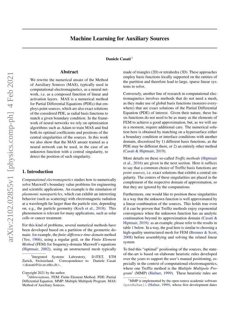
Figure 1 shows three examples of multipoles according to(3) with center c = 0.

-1 -0.5 0 0.5 1

-1

-0.8

-0.6

-0.4

-0.2

0

0.2

0.4

0.6

0.8

1

-4.5

-4

-3.5

-3

-2.5

-2

-1.5

-1

-0.5

0

(a) log ρ

-1 -0.5 0 0.5 1

-1

-0.8

-0.6

-0.4

-0.2

0

0.2

0.4

0.6

0.8

1

-0.01

-0.005

0

0.005

0.01

(b) ρ−2 cos(2θ) (c) ρ−3 cos(3θ)

Figure 1. Sample multipoles according to (3), i.e. discrete basisfunctions of the MMP Trefftz space (2).

Each multipole from (3) is characterized by a location, i.e.its center c, and the parameter j (its degree), which canbe assumed 0 for the case log ρxc. When we place severalmultipoles at a given location up to a certain order p, whichis the maximum degree of multipoles with that center, weuse the term multipole expansion. Summing the number ofterms of all multipole expansions used for approximation(each with a different center) yields the total number ofdegrees of freedom of the discretized Trefftz space T n(Ω)from (2).

Once a discrete basis of multipoles has been chosen, thereare several ways to find their coefficients such that the errorwith the boundary condition is minimized (Hiptmair et al.,2016): the most common is arguably collocation on selectedmatching points of the hypersurface (Hafner, 1980), whichaims at minimizing the `2-error at the matching points in aleast-squares sense.

In this work we propose to use a gradient-based optimiza-tion algorithm, typically employed to train neural networksthat have many degrees of freedom, to optimize with respectto both the coefficients of the multipoles and the centers oftheir singularities. In other words, we do not preselect thecenters and then find the corresponding optimal coefficients,in a similar way to precomputing a finite-element mesh, butwe optimize both at the same time. This is doable becausethe number of centers scales logarithmically with respectto the number of matching points used for collocation, con-sidering the exponential convergence of MMP (Casati &Hiptmair, 2019).

4This condition is here unnecessary, as we work with a boundedΩ to compute L2(Ω)-errors for validation.

Machine Learning for Auxiliary Sources

3. MMP as a Neural NetworkIn this section we rewrite the numerical ansatz of MMP asa neural network, i.e. as a composed function of linear andactivation layers. In this way, we are able to rely on effi-cient implementations of popular optimization algorithmsfor neural networks, such as the Adam algorithm (Kingma& Ba, 2015), as well as the automatic differentiation (Rall,1981) component of these implementations.

The MMP ansatz approximates an unknown function asfollows:

n∑i=1

pi∑j=0

wijfij(x− ci), (5)

where

• n is the number of multipole expansions,

• pi is the order of the i-th multipole expansion, i.e. weconsider terms in (3) from j = 0 (corresponding tolog ρxc) to pi, and

• wij ∈ R is the coefficient of fij(x − ci) ∈ T n(Ω),with x, ci ∈ R2 and ci center of the i-th multipoleexpansion.

Following the formalism of neural networks (Haykin, 2008),we can rewrite (5) as a 3-layer neural network, given x ∈ R2

as the input variable:

1. The first linear layer is represented by the followingaffine transformation with a nonzero shift:

x 7→

I2,2...

I2,2

p1

...I2,2

...I2,2

pn

x−

c1...c1

p1

...cn...cn

pn

= u ∈ R2m,

(6)where m :=

∑ni=1(pi + 1) and the shift (bias) is made

of the centers of the multipoles, to be determined bythe optimization.

2. The activation layer is composed of several “many-to-one” activation functions, as they map pairs of vari-ables to a single one:

f(u) = v ∈ Rm, (7)

where each activation function fij : R2 → R, j =0, . . . , pi, i = 1, . . . , n, is a multipole. Examples of“many-to-one” activation functions from the literatureof neural networks include softmax, max pooling, max-out, and gating (Ramachandran et al., 2017).

3. Finally, the third layer is linear without bias:

w> · v = y ∈ R, (8)

where the weights w ∈ Rm are the coefficients of themultipole expansions.

Figure 2 schematizes the neural network representation ofthe MMP ansatz described above.

𝑥1𝑥2

𝑝1

𝑥1 − 𝑐1(1)

𝑥2 − 𝑐2(1)

⋮

𝑥1 − 𝑐1(1)

𝑥2 − 𝑐2(1)

𝑝𝑛

𝑥1 − 𝑐1(𝑛)

𝑥2 − 𝑐2(𝑛)

⋮

𝑥1 − 𝑐1(𝑛)

𝑥2 − 𝑐2(𝑛)

⋮

𝑓0(1)

𝒙 − 𝒄(1)

⋮

𝑓𝑝1(1)

𝒙 − 𝒄(1)

𝑓0(𝑛)

𝒙 − 𝒄(𝑛)

⋮

𝑓𝑝𝑛(𝑛)

𝒙 − 𝒄(𝑛)

⋮

𝑗=0

𝑝1

𝑤𝑗𝑓𝑗(1)

𝒙 − 𝒄(1)

𝑗=0

𝑝𝑛

𝑤𝑗𝑓𝑗(𝑛)

𝒙 − 𝒄(𝑛)

⋮

𝑖=1

𝑛

𝑗=0

𝑝𝑖

𝑤𝑗(𝑖)𝑓𝑗(𝑖)

𝒙 − 𝒄(𝑖)

InputWidth: 2

Repetition + BiasWidth: 2σ𝑖=1

𝑛 𝑝𝑖

ActivationWidth: σ𝑖=1

𝑛 𝑝𝑖

Linear

Figure 2. Neural network representation of the MMP ansatz.

Based on this representation, one can see that the centersof singularities ci, i = 1, . . . , n, are, together with thecoefficients wij , j = 0, . . . , pi, degrees of freedom of thisneural network. The total number of degrees of freedom is2n +

∑ni=1(pi + 1): note that, in case of few high-order

multipole expansions, the additional degrees of freedomconstituted by their centers (2n) do not have much impacton the total number.

For the loss function of this neural network we follow thecollocation method, whose goal is to minimize the `2(Γ)-error between the MMP ansatz (5) and the boundary condi-tion on the chosen matching points:

L(c,w) :=

N∑l=1

n∑i=1

pi∑j=0

wijfij(xl − ci)− yl

2

, (9)

where yl, l = 1, . . . , N , are the evaluations of the unknown(assuming a Dirichlet boundary condition) on the N match-ing points xl.

4. Numerical ResultsAs bounded domain Ω for a 2D Poisson’s problem wechoose the interior region of a flower-shaped curve Γ := ∂Ω,parameterized by the formula

(R(θ) cos θ,R(θ) sin θ)>, R(θ) = α(β + γ cos(Kθ))

(10)in Cartesian coordinates, with θ ∈ [0, 2π), α, β, γ ∈ R, andK ∈ N. We set α = 0.5, β = 1, γ = 0.5, and K = 5,

Machine Learning for Auxiliary Sources

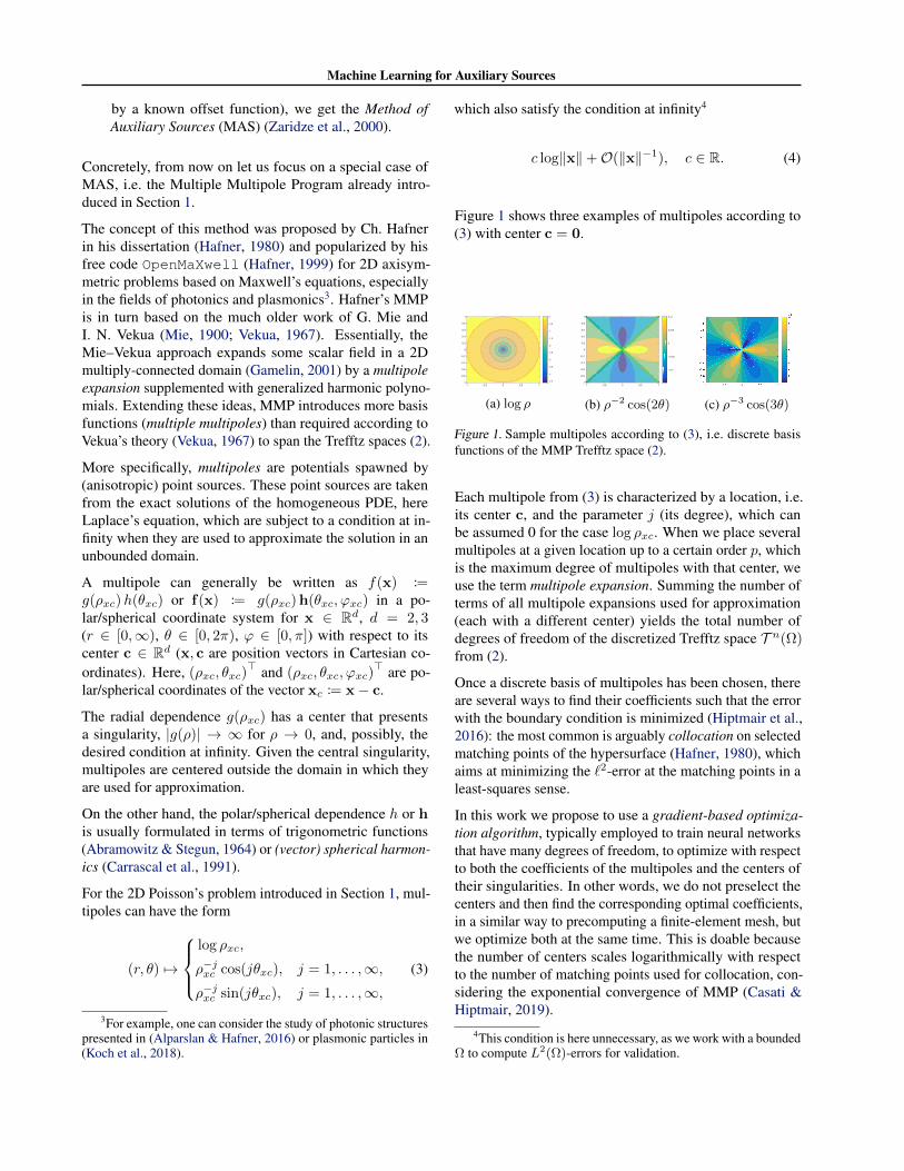
and choose N = 100 points of Γ from equidistant values ofθ ∈ [0, 2π) to serve as matching points.

Figure 3a shows the flower-shaped curve according to (10),Figure 3b the meshed domain with triangles. This meshis used to compute the L2(Ω)-error of the MMP approxi-mation with respect to manufactured solutions of type (1)(see Section 1) with different centers σ ∈ R2 \ Ω. For thenumerical quadrature of the error, we employ the Gaussianquadrature rule of order 5 (polynomials up to the 5-th orderare integrated exactly) on triangles.

−1.0 −0.5 0.0 0.5 1.0

−1.

0−

0.5

0.0

0.5

1.0

(a) Flower-shaped curve ac-cording to (10) (100 matchingpoints).

(b) Sample mesh of theflower-shaped domain.

Figure 3. Flower-shaped curve and sample mesh.

In the following we discuss two experiments solving thisboundary value problem with MMP: first, we investigate thedependence of the Adam optimization on the number of mul-tipole expansions used for approximation (Section 4.1), thenon the order of a single multipole expansion (Section 4.2).

4.1. Dependence on the number of multipoleexpansions

With the Adam algorithm we find the coefficients and cen-ters of singularities of the MMP expansions that minimizethe boundary `2(Γ)-error with a manufactured solution onselected matching points. The “dataset” to train the MMPansatz as a neural network is made of coordinates of match-ing points as input observations and the corresponding eval-uations of the manufactured solution as output.

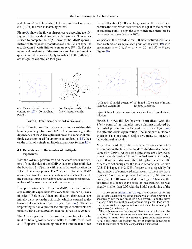
To approximate (1), we choose an MMP ansatz made of sev-eral multipole expansions (we vary their number n), eachof order 1. Before the Adam optimization, their centers areinitially disposed on the unit circle, which is external to thebounded domain Ω of Figure 3 (see Figure 4a). The cor-responding initial values for the multipole coefficients areobtained from the collocation method, given these centers.

The Adam algorithm is then run for a number of epochsuntil the training loss becomes smaller than 0.05, for at most5 · 105 epochs. The learning rate is 0.1 and the batch size

is the full dataset (100 matching points): this is justifiedbecause the number of observations is equal to the numberof matching points, set by the user, which must therefore behumanely manageable (here 100).

We perform this procedure for 100 manufactured solutions,each centered on an equidistant point of the curve (10) withparameters α = 0.8, β = 1, γ = 0.2, and K = 5 (seeFigure 4b).

−1.0 −0.5 0.0 0.5 1.0

−1.

0−

0.5

0.0

0.5

1.0

(a) In red, 10 initial centers ofmultipole expansions.

−1.0 −0.5 0.0 0.5 1.0

−1.

0−

0.5

0.0

0.5

1.0

(b) In red, 100 centers of manu-factured solutions.

Figure 4. Initial centers of multipoles and centers of manufacturedsolutions.

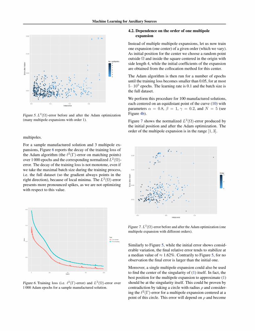
Figure 5 shows the L2(Ω)-error (normalized with theL2(Ω)-norm of the manufactured solution) produced bythe initial positioning on the unit circle5 (see Figure 4a)and after the Adam optimization. The number of multipoleexpansions is in the range [3, 9] to investigate its impact onthe optimization result.

Notice that, while the initial relative error shows consider-able variation, the final error tends to stabilize at a medianvalue of ≈ 0.98%. At the same time, there are a few caseswhere the optimization fails and the final error is noticeablylarger than the initial one: they take place when 5 · 105

epochs are not enough for the loss to become smaller than0.05. This happens in 2.17% of observations, especially forhigh numbers of considered expansions, as there are moredegrees of freedom to optimize. Furthermore, 101 observa-tions (out of 700) are excluded from Figure 5 because theoptimization stopped at the first step: the training loss wasalready smaller than 0.05 with the initial positioning of the

5As proven in (Sakakibara, 2016), if the solution (1) of the2D Poisson’s equation possesses an analytic extension beyond Ω,specifically into the region of R2 \ Ω between Γ and the curveΣ along which the multipole expansions are placed, then we ex-pect exponential convergence in terms of the number of multipoleexpansions (or their orders).

This is however not the case of Figure 4a, which shows theunit circle Σ in red, given the solutions with the centers shownin Figure 4a. In this way, the proposed approach is tested for aninitial positioning that does not present exponential convergencewhen the number of multipole expansions is increased.

Machine Learning for Auxiliary Sources

0.01

0.03

0.10

0.30

0.0 0.1 0.2 0.3Initial error

Err

or a

fter

Ada

m

3

4

5

6

7

8

9No. multipoles

Figure 5. L2(Ω)-error before and after the Adam optimization(many multipole expansions with order 1).

multipoles.

For a sample manufactured solution and 3 multipole ex-pansions, Figure 6 reports the decay of the training loss ofthe Adam algorithm (the `2(Γ)-error on matching points)over 1 000 epochs and the corresponding normalized L2(Ω)-error. The decay of the training loss is not monotone, even ifwe take the maximal batch size during the training process,i.e. the full dataset (so the gradient always points in theright direction), because of local minima. The L2(Ω)-errorpresents more pronounced spikes, as we are not optimizingwith respect to this value.

0.05

0.10

0.15

0.20

0 250 500 750 1000Epoch

Err

or

Type

L^2 in domain

l^2 on boundary

Figure 6. Training loss (i.e. `2(Γ)-error) and L2(Ω)-error over1 000 Adam epochs for a sample manufactured solution.

4.2. Dependence on the order of one multipoleexpansion

Instead of multiple multipole expansions, let us now trainone expansion (one center) of a given order (which we vary).As initial position for the center we choose a random pointoutside Ω and inside the square centered in the origin withside length 4, while the initial coefficients of the expansionare obtained from the collocation method for this center.

The Adam algorithm is then run for a number of epochsuntil the training loss becomes smaller than 0.05, for at most5 · 105 epochs. The learning rate is 0.1 and the batch size isthe full dataset.

We perform this procedure for 100 manufactured solutions,each centered on an equidistant point of the curve (10) withparameters α = 0.8, β = 1, γ = 0.2, and N = 5 (seeFigure 4b).

Figure 7 shows the normalized L2(Ω)-error produced bythe initial position and after the Adam optimization. Theorder of the multipole expansion is in the range [1, 3].

0.01

0.03

0.10

0.30

0.0 0.5 1.0Initial error

Err

or a

fter

Ada

m

1

2

3Order

Figure 7. L2(Ω)-error before and after the Adam optimization (onemultipole expansion with different orders).

Similarly to Figure 5, while the initial error shows consid-erable variation, the final relative error tends to stabilize ata median value of ≈ 1.62%. Contrarily to Figure 5, for noobservation the final error is larger than the initial one.

Moreover, a single multipole expansion could also be usedto find the center of the singularity of (1) itself. In fact, thebest position for the multipole expansion to approximate (1)should be at the singularity itself. This could be proven bycontradiction by taking a circle with radius ρ and consider-ing the `2(Γ)-error for a multipole expansion centered at apoint of this circle. This error will depend on ρ and become

Machine Learning for Auxiliary Sources

minimal when ρ = 0.

Figure 8 shows the `2-distance between the singularity of thesolution and the center of one multipole expansion beforeand after the Adam optimization. In 12.16% of observationsthe initial distance is smaller than the one after the Adamoptimization: however, in all these cases the training lossdid not become smaller than 0.05 in 5 · 105 epochs.

1e−03

1e−02

1e−01

1e+00

1e+01

0 1 2 3Initial distance

Dis

tanc

e af

ter

Ada

m

1

2

3Order

Figure 8. `2-distance between solution and expansion before andafter the Adam optimization (one multipole expansion with differ-ent orders).

4.3. Implementation

Our code is written in Python 3.

For meshing and numerical integration, we rely onNetgen/NGSolve (TU Wien, 2019). For the Adam op-timization, we rely on PyTorch (Facebook AI Research,2020). By defining a new torch.nn.Module for the firstand second layer of the MMP ansatz as a neural network(Section 3), we can use the automatic differentiation toolof PyTorch for the Jacobians needed by the backpropaga-tion step of the Adam algorithm. Furthermore, we exploitthe PyTorch parallelization on GPUs when training eachneural network and the Python multiprocessing module toparallelize over the manufactured solutions.

5. ConclusionsWe have shown that gradient-based optimization algorithmscommonly used to train neural networks, such as the Adamalgorithm, can help with overcoming a flaw of MAS, namelythe heuristics needed to place its point sources, by opti-mizing with respect to these positions (together with thecoefficients of the point sources).

Future work will involve 1) applying this approach to otherproblems, i.e. with different boundaries, manufactured so-lutions, and PDEs, and 2) using a genetic algorithm to op-timize also with respect to the number and orders of themultipole expansions (total number of degrees of freedomof MMP). These are the metaparameters of the MMP ansatzas a neural network, which now have to be chosen by theuser. A too large number of degrees of freedom for MMPshould be penalized by the genetic procedure.

ReferencesAbramowitz, M. and Stegun, I. A. Handbook of Mathemati-

cal Functions with Formulas, Graphs, and MathematicalTables. Dover, New York, NY, 9th edition, 1964.

Alparslan, A. and Hafner, C. Current status of MMP anal-ysis of photonic structures in layered media. In 2016IEEE/ACES International Conference on Wireless Infor-mation Technology and Systems (ICWITS) and AppliedComputational Electromagnetics (ACES), pp. 1–2, 2016.doi: 10.1109/ROPACES.2016.7465317.

Brenner, S. C. and Scott, L. R. The Mathematical Theory ofFinite Element Methods, volume 15 of Texts in AppliedMathematics. Springer, New York, NY, 3rd edition, 2008.doi: 10.1007/978-0-387-75934-0.

Carrascal, B., Estevez, G., Lee, P., and Lorenzo, V. Vec-tor spherical harmonics and their application to classicalelectrodynamics. European Journal of Physics, 12(4):184–191, 1991. doi: 10.1088/0143-0807/12/4/007.

Casati, D. and Hiptmair, R. Coupling finite elements andauxiliary sources. Computers & Mathematics with Appli-cations, 77(6):1513–1526, 2019.

Facebook AI Research. PyTorch v17.0, 2020. URL https://pytorch.org.

Gamelin, T. W. Complex Analysis. Undergraduate Texts inMathematics. Springer, New York, NY, 1st edition, 2001.doi: 10.1007/978-0-387-21607-2.

Griffiths, D. J. Introduction to Electrodynamics. Pearson,Boston, MA, 4th edition, 2013. Republished by Cam-bridge University Press in 2017.

Hafner, C. Beitrage zur Berechnung der Ausbreitungelektromagnetischer Wellen in zylindrischen Strukturenmit Hilfe des “Point-Matching”-Verfahrens. PhD the-sis, ETH Zurich, Switzerland, 1980. URL https://doi.org/10.3929/ethz-a-000220926.

Hafner, C. Chapter 3 - The Multiple Multipole Pro-gram (MMP) and the Generalized Multipole Technique(GMT). In Wriedt, T. (ed.), Generalized Multipole

Machine Learning for Auxiliary Sources

Techniques for Electromagnetic and Light Scattering,pp. 21–38. Elsevier, Amsterdam, 1999. doi: 10.1016/B978-044450282-7/50015-4.

Haykin, S. Neural Networks and Learning Machines. Pear-son, 3rd edition, 2008.

Heretakis, I. I., Papakanellos, P. J., and Capsalis, C. N.A stochastically optimized adaptive procedure for thelocation of mas auxiliary monopoles: the case of electro-magnetic scattering by dielectric cylinders. IEEE Trans-actions on Antennas and Propagation, 53(3):938–947,2005. doi: 10.1109/TAP.2004.842699.

Hiptmair, R. Finite elements in computational electro-magnetism. Acta Numerica, 11, 2002. doi: 10.1017/S0962492902000041.

Hiptmair, R., Moiola, A., and Perugia, I. A survey of Trefftzmethods for the Helmholtz equation. In Barrenechea,G. R., Brezzi, F., Cangiani, A., and Georgoulis, E. H.(eds.), Building Bridges: Connections and Challengesin Modern Approaches to Numerical Partial DifferentialEquations, pp. 237–279. Springer, Cham, 2016. doi:10.1007/978-3-319-41640-3 8.

Kingma, D. P. and Ba, J. Adam: A method for stochas-tic optimization. In Bengio, Y. and LeCun, Y. (eds.),3rd International Conference on Learning Represen-tations, ICLR 2015, San Diego, CA, USA, May 7–9,2015, Conference Track Proceedings, 2015. URL http://arxiv.org/abs/1412.6980.

Koch, U., Niegemann, J., Hafner, C., and Leuthold, J. MMPsimulation of plasmonic particles on substrate under e-beam illumination. In Wriedt, T. and Eremin, Y. (eds.),The Generalized Multipole Technique for Light Scatter-ing: Recent Developments, pp. 121–145. Springer, Cham,2018. doi: 10.1007/978-3-319-74890-0 6.

Kupradze, V. D. and Aleksidze, M. A. The method of func-tional equations for the approximate solution of certainboundary value problems. USSR Computational Math-ematics and Mathematical Physics, 4(4):82–126, 1964.doi: 10.1016/0041-5553(64)90006-0.

Mie, G. Elektrische Wellen an zwei parallelen Drahten.Annalen der Physik, 307:201–249, 1900. doi: 10.1002/andp.19003070602.

Moiola, A. Trefftz-Discontinuous Galerkin Methods forTime-Harmonic Wave Problems. PhD thesis, Seminarfor Applied Mathematics, ETH Zurich, Switzerland,2011. URL https://www.doi.org/10.3929/ethz-a-006698757.

Moreno, E., Erni, D., Hafner, C., and Vahldieck, R. Mul-tiple multipole method with automatic multipole settingapplied to the simulation of surface plasmons in metallicnanostructures. Journal of the Optical Society of AmericaA, 19(1):101–111. doi: 10.1364/JOSAA.19.000101.

Rall, L. B. Automatic differentiation: Techniques and ap-plications, volume 120 of Lecture Notes in ComputerScience. Springer, 1st edition, 1981. doi: 10.1007/3-540-10861-0.

Ramachandran, P., Zoph, B., and Le, Q. V. Searching for ac-tivation functions. Computing Research Repository, 2017.URL http://arxiv.org/abs/1710.05941.

Sakakibara, K. Analysis of the dipole simulation methodfor two-dimensional Dirichlet problems in Jordan regionswith analytic boundaries. BIT Numerical Mathematics, 56(4):1369–1400, 2016. doi: 10.1007/s10543-016-0605-1.

TU Wien. Netgen/NGSolve v6.2, 2019. URL https://ngsolve.org.

Vekua, I. N. New Methods for Solving Elliptic Equations.North Holland Publishing Company, 1st edition, 1967.

Yee, K. Numerical solution of initial boundary value prob-lems involving Maxwell’s equations in isotropic media.IEEE Transactions on Antennas and Propagation, 14(3):302–307, 1966. doi: 10.1109/TAP.1966.1138693.

Zaridze, R. S., Bit-Babik, G., Tavzarashvili, K., Uzunoglu,N. K., and Economou, D. P. The Method of Auxil-iary Sources (MAS) — Solution of propagation, diffrac-tion and inverse problems using MAS. In Uzunoglu,N. K., Nikita, K. S., and Kaklamani, D. I. (eds.), Ap-plied Computational Electromagnetics: State of the Artand Future Trends, volume 171 of NATO ASI Series,pp. 33–45. Springer, Berlin, Heidelberg, 2000. doi:10.1007/978-3-642-59629-2 3.