machine learning: decision trees and random forests - jo£o aires de

1

1st Session

Machine learning: decision trees and

random forests

2

Can a computer learn chemistry ?

3

For example, learn to predict properties from the molecular structural formula

Learn what ?

Is it toxic ?

How does it react with a

base ?

How are its spectra (IR,

NMR, MS,...) ?CH3

CH3

O

O

Pharmacological properties ?

4

Empirically !

A computer can learn, just like experimental chemists have typically learned...

Starting from a dataset of experimental data with molecular structures and the corresponding observable properties.

A computer can find relationships between molecular structures and the properties.

It learns! And can apply the knowledge to new situations!

5

Structure – property relationships

Computers typically work with numbers...

Molecular

structurePropertiesRepresentation

Machine

learning

CH3

CH3

O

NH Moleculardescriptors

(numbers!)

• Neural networks

• Decision trees

• Regressions

• ...

Physical

Chemical

Biological

6

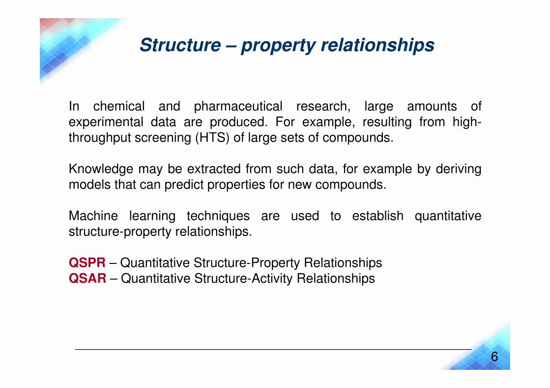
Structure – property relationships

In chemical and pharmaceutical research, large amounts of experimental data are produced. For example, resulting from high-throughput screening (HTS) of large sets of compounds.

Knowledge may be extracted from such data, for example by deriving models that can predict properties for new compounds.

Machine learning techniques are used to establish quantitativestructure-property relationships.

QSPR – Quantitative Structure-Property RelationshipsQSAR – Quantitative Structure-Activity Relationships

7

8.00

9.00

10.00

11.00

12.00

13.00

14.00

15.00

16.00

8.00 9.00 10.00 11.00 12.00 13.00 14.00 15.00 16.00 17.00

Multilinear regressions

Variables x1, x2, x3, x4, … xn Variable y

Find the equation that best expresses the linear relationship between x1,… xn and y.

y = a1 x1 + a2 x2 + a3 x3 + a4 x4 + … + an xn + b

The goal is to find the best possible values of a1 … an and b such that the equation allows to predict y from X.

The least squares algorithm minimizes the sum of the squared distances of the points to the line in an n dimensional space.

experimental

pre

dic

ted

8

Multilinear regressionsApplication to QSPR

Descriptors x1, x2, x3, x4, … xn Property y

To find an equation that can predict the property y from descriptorsx1,… xn.

It is wise to look for descriptors that are expected to be related to the property.

For example, the melting point is related to the size and polarity of compounds; if we want to model mp we should use molecular descriptors encoding size and polarity.

9

8.00

9.00

10.00

11.00

12.00

13.00

14.00

15.00

16.00

8.00 9.00 10.00 11.00 12.00 13.00 14.00 15.00 16.00 17.00


Example: prediction of the rate constant of the reaction of a compound with the OH radical

-logk(OH) = 5.00 – 0.68 HOMO + 0.35 nX –

– 0.39 CIC0 + 0.13 nCaH

Training set

234 objects (compounds)

HOMO – Energy of the highest occupied molecular orbital

nX – number of halogen atoms

CIC0 – a complementaryinformation content index,

nCaH – number of unsubstitutedaromatic C (sp2)

P.Gramatica, P. Pilutti, E. Papa,J. Chem. Inf. Comput. Sci. 2004, 44, 1794-1802 experimental

pre

dic

ted

10

8.00

9.00

10.00

11.00

12.00

13.00

14.00

15.00

16.00

8.00 9.00 10.00 11.00 12.00 13.00 14.00 15.00 16.00

-logk(OH) = 5.00 – 0.68 HOMO + 0.35 nX –

– 0.39 CIC0 + 0.13 nCaH

Test set

226 compounds

experimental


Example: prediction of the rate constant of the reaction of a compound with the OH radical

HOMO – Energy of the highest occupied molecular orbital

nX – number of halogen atoms

CIC0 – a complementaryinformation content index,

nCaH – number of unsubstitutedaromatic C (sp2)

pre

dic

ted

11

Decision trees(or classification and regression trees, CART)

Descriptors x1, x2, x3, x4, … xn Classes A, B, C, …

� Decision trees build rules that are able to classify

objects on the basis of descriptors x1,… xn.

� Rules are inferred from objects in the training set. After

training, the trees can be applied to new objects for their

classification.

12


A non-parametric technique that produces either

classification or regression trees, depending on whether the

dependent variable is categorical or numeric, respectively.

Trees are formed by a collection of rules based on values of

attributes (variables) in the training data set

Wikipedia

13


� Rules are selected based on how well splits based on

variables’ values can differentiate observations based

on the dependent variable.

� Once a rule is selected and splits a node into two, the

same logic is applied to each “child” node (i.e. it is a

recursive procedure).

� Splitting stops when no further gain can be made, or

some pre-set stopping rules are met.

Wikipedia

14


Each branch of the tree ends in a terminal node.

Classification: each terminal node is classified according

to the majority of objects falling into it.

Regression: each terminal node is associated with a

numerical prediction – the average of the dependent

variable of the objects falling into it.

15

Decision trees

Example: prediction of mutagenicityfrom 381 molecular descriptors

32 polycyclic aromatic hydrocarbons (PAH)

Gs≥0.3325< 0.3325

Gs≥0.2045< 0.2045

R5m+≥0.015< 0.015

Mut MutNon-Mut Non-Mut

Gs: G total symmetry index/weighted by atomic electrotopological states (3D-WHIM descriptor)

R5m+: R maximal autocorrelation of lag 5/weighted by atomic masses (3D-GETAWAY descriptor)

P. Gramatica, E. Papa, A. Marrocchi, L. Minuti, A. Taticchi, Ecotoxicology and Environmental Safety 2007, 66 (3), 353-361.

‘Leave-one-out’ validation: 3/32 wrong classifications

16

Decision treeExample: Prediction of CYP3A4 inhibition

� Data set:

Training set: 741 compounds(273 CYP3A4 inhibitors and 468 non-inhibitors)

Test set: 186 compounds(121 CYP3A4 inhibitors and 65 non-inhibitors)

� 240 Molecular descriptors: (1) constitutional descriptors like

formal charges, fraction of rotatable bonds, number of rigid bonds, number of rings, number of charged groups, etc., (2) electrostatic descriptors that include charge polarization, relative charge, etc., (3) physicochemical descriptors like AlogP98 value, and (4) geometrical descriptors containing information from the 3D structure of a compound, such as the polar surface area.

I. Choi, S. Y. Kim, H. Kim, N. S. Kang, M. A. Bae, S.-E. Yo, J. Jung, K. T. No, Eur. J. Med. Chem. 2009, 44, 2354–2360.

17

The classified number of inhibitors and non-inhibitors for training set (black) and test set (purple) is shown in parentheses.

Decision tree prediction of CYP3A4 inhibition

18

Results

53.85 (35/65)82.64 (100/121)72.58 (135/186)Test

70.3 (329/468)75.82 (207/273)72.33 (536/741)Training

Specificity, %Sensitivity, %Accuracy, %Data set


19


Selected molecular descriptors

Fraction of 2D van der Waals hydrophobic of surface areaFraction of 2D_VSA hydrophobic

Fraction of 2D van der Waals chargeable groups of surface areaFraction of 2D VSA chargeable groups

Geometric

The partial positive VDW surface area divided by the total VDW surface area

FPSA1

The difference between total charge weighted partial positive and negative surface areas

DPSA2

Electrostatic

The number of single bonds between C atoms and C atomsNo_CsH

The number of double bonds between C atoms and C atomsNo_CdC

The number of amine groupsNo_amine_groups

Molecular weightMolecular_weight

Constitutional

RepresentationNameDescriptor group

20

Why CART is a successful tool?

1. Universally applicable to classification and regression problems with no assumptions on the data structure.

2. The picture of the tree structure gives valuable insights into which variables were important and where.

3. Terminal nodes gave a natural clustering of the data into homogenous groups.

4. Handles missing data and categorical variables efficiently.

5. Can handle large data sets—computational requirements are order of MNlogN where N is number of cases and M is number of variables.

http://stat-www.berkeley.edu/users/breiman/RandomForests/

21

Drawbacks of CART

accuracy: current methods such as SVMs average

30% lower error rates than CART.

instability: change the data a little and you get a

different tree picture. So the interpretation of

what goes on is built on shifting sands.

http://stat-www.berkeley.edu/users/breiman/RandomForests/

22

Random Forests (RF)

Random Forests grows many classification trees and predictions are

made by majority vote of the individual trees.

RootRoot

RootRoot

23

Random Forest

� Random Forests grows many classification trees.

� To classify a new object from an input vector, put the input vector down each of the trees in the forest.

� Each tree gives a classification – the tree "votes" for that class.

� The forest chooses the classification having the most

votes (over all the trees in the forest).

Leo Breiman and Adele Cutlerhttp://stat-www.berkeley.edu/users/breiman/RandomForests/

24

Random Forest

Each tree is grown as follows:

1. If the number of cases in the training set is N, sample N cases at random - but with replacement, from the original data. This sample

will be the training set for growing the tree.

2. If there are M input variables, a number m<<M is specified such that at each node, m variables are selected at random out of the M and the best split on these m is used to split the node. The value of m is

held constant during the forest growing.

3. Each tree is grown to the largest extent possible. There is no pruning.

25

Random Forest

The forest error rate depends on two things:

1. The correlation between any two trees in the forest. Increasing the correlation increases the forest error rate.

2. The strength of each individual tree in the forest. A tree with a low error rate is a strong classifier. Increasing the strength of the individual trees decreases the forest error rate.

Reducing m reduces both the correlation and the strength. Increasing it increases both.

26

Random Forest

The out-of-bag (oob) error estimate

No need for cross-validation or a separate test set to get an unbiased estimate ofthe test set error.

� Each tree is constructed using a different bootstrap sample from the original data.

� Each tree predicts the objects left out of its growing.

� Errors for all objects left out in all trees produce an error estimate – OOB error estimate.

27

Random Forest

Random Forest (RF) is an ensemble of unpruned classification

trees with predictions made by majority vote of the individual trees.

� Probability: number of votes obtained by the predicted class.

� Variable importance

� Similarity between two compounds: assessed by the

number of times they are classified in the same terminal nodes of the RF individual trees.

28

Similarity assessed by Random Forests

In 2 out of 4 trees of the forest, objects b1 and b2 fall in the same terminal node - their similarity is 2/4 = 0.5.

Root

b1

b2

Root

b1,b2

Root

b1

b2

Root

b1,b2

29

Features of Random Forests

� It is amongst the most accurate of current algorithms.

� It runs efficiently on large data bases.

� It can handle thousands of input variables without variable

deletion.

� It gives estimates of what variables are important in the

classification.

� It generates an internal unbiased estimate of the

generalization error as the forest building progresses.

� It has methods for balancing error in class population unbalanced data sets.

30

Features of Random Forests

� Generated forests can be saved for future use on other data.

� Prototypes are computed that give information about the

relation between the variables and the classification.

� It computes proximities between pairs of cases that can be

used in clustering, locating outliers, or (by scaling) give

interesting views of the data.

� The capabilities of the above can be extended to unlabeled

data, leading to unsupervised clustering, data views and outlier

detection.

� It offers an experimental method for detecting variable

interactions.

31

RF prediction of mutagenicity (Ames test)

• Training set: 4083 structures (57% positive, 43% negative)

• Test set: 472 structures (65% positive, 35% negative)

• Descriptors:

• MOLMAPs of dimension 25×25

• 17 global molecular descriptors

• Machine learning method: Random Forest

Q.-Y. Zhang, J. Aires-de-Sousa, J. Chem. Inf. Model. 2007, 47(1), 1-8.

32

Results(correct predictions)

91%

85%

Test set

(472 structures)

Only predictions with

probability ≥ 0.7

(296 structures)

All structures

Training set*

(4083 structures)

-

84%

* Internal cross-validation by out-of-bag estimation.

Inter-laboratory experimental error: 15%

33

Results for the test set

0.93

0.86

Specificity

0.91

0.84

Sensitivity

91%(296 out of

324 structures)

MOLMAPs 25×25 + 17 GMD (only predictions with

probability ≥ 0.7)

85%MOLMAPs 25×25 + 17 GMD

Correct predictionsDescriptors

Sensitivity: Ratio of true positives to the sum of true positives and false negatives.

Specificity: Ratio of true negatives to the sum of true negatives and false positives.

34

Receiver Operator Characteristic (ROC) curve

0

0.1

0.2

0.3

0.4

0.5

0.6

0.7

0.8

0.9

1

0 0.2 0.4 0.6 0.8 1

1 - Specificity (false positives)

Sen

sit

ivit

y (

tru

e p

osit

ives)

No discrimination

Predict

ROC for the 472 test compounds. Area = 0.914

35

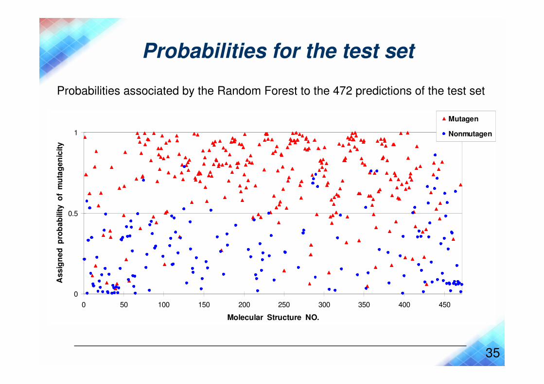
Probabilities for the test set

Probabilities associated by the Random Forest to the 472 predictions of the test set

0

0.5

1

0 50 100 150 200 250 300 350 400 450

Molecular Structure NO.

As

sig

ne

d p

rob

ab

ilit

y o

f m

uta

ge

nic

ity

Mutagen

Nonmutagen

36

False negatives

False negatives predicted with low probability (<0.1)

Predicted non-mutagens, but listed as mutagens

Most similar compounds in the training set

OO

O

A 9

O

OO

OO

A 1 1

OO

O O

A 1 0

OOO O

OOH O

OH

OO

OHO

OOH OH OH

OH

OH

OH

OH

OH

O

OH OH

37

S P

O

O

O

S P

O

O

S

O

S

P

S

O

S

O

S

P

OO

O O

O

O

Predicted non-mutagens, but listed as mutagens

Most similar compounds in the training set

OH

O

OH

OO

O

False negatives

False negatives predicted with low probability (<0.1)

38

Most important descriptors

• MOLMAP components associated with N-O bonds

• GMD min/max charge on a H atom

• GMD ring strain energy

Relative importance of descriptors

39

Random Forests with 200 trees

Correct predictions

84%

84%

84%

Training set (OOB)

0.87

0.86

0.87

Specificity

0.8183%The 50 most important descriptors

0.8484%The 100 most important descriptors

0.8384%642 descriptors

SensitivityCorrect

predictions

Test set

Descriptors

40

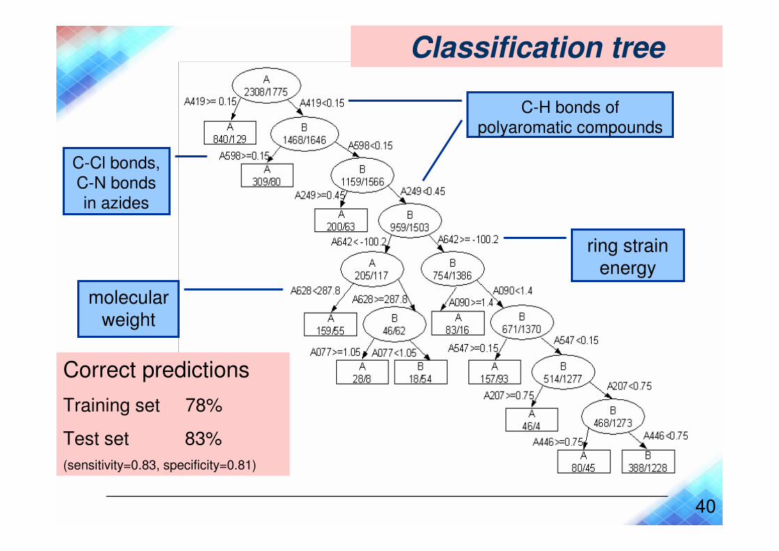
Classification tree

C-H bonds of

polyaromatic compounds

C-Cl bonds,

C-N bonds

in azides

molecular weight

ring strain energy

Correct predictions

Training set 78%

Test set 83%

(sensitivity=0.83, specificity=0.81)

41

Web interfaceInput SMILES string

42

Web interfaceOutput for one structure

43

Web interfaceInput several SMILES strings

44

Web interfaceOutput for several structures

45

Web interfaceSimilarities in the training set

46


47


machine learning: decision trees and random forests - jo£o aires de

Documents