Machine Learning Classification over Encrypted Data

Raphaël Bost∗ Raluca Ada Popa†‡ Stephen Tu‡ Shafi Goldwasser‡

Abstract

Machine learning classification is used in numerous settings nowadays, such as medical or genomics predictions,spam detection, face recognition, and financial predictions. Due to privacy concerns, in some of these applications, it isimportant that the data and the classifier remain confidential.

In this work, we construct three major classification protocols that satisfy this privacy constraint: hyperplanedecision, Naïve Bayes, and decision trees. We also enable these protocols to be combined with AdaBoost. At the basisof these constructions is a new library of building blocks for constructing classifiers securely; we demonstrate that thislibrary can be used to construct other classifiers as well, such as a multiplexer and a face detection classifier.

We implemented and evaluated our library and classifiers. Our protocols are efficient, taking milliseconds to a fewseconds to perform a classification when running on real medical datasets.

1 IntroductionClassifiers are an invaluable tool for many tasks today, such as medical or genomics predictions, spam detection, facerecognition, and finance. Many of these applications handle sensitive data [WGH12, SG11, SG13], so it is importantthat the data and the classifier remain private.

Consider the typical setup of supervised learning, depicted in Figure 1. Supervised learning algorithms consist oftwo phases: (i) the training phase during which the algorithm learns a model w from a data set of labeled examples,and (ii) the classification phase that runs a classifier C over a previously unseen feature vector x, using the model w tooutput a prediction C(x,w).

In applications that handle sensitive data, it is important that the feature vector x and the model w remain secret toone or some of the parties involved. Consider the example of a medical study or a hospital having a model built out ofthe private medical profiles of some patients; the model is sensitive because it can leak information about the patients,and its usage has to be HIPAA1 compliant. A client wants to use the model to make a prediction about her health (e.g.,if she is likely to contract a certain disease, or if she would be treated successfully at the hospital), but does not wantto reveal her sensitive medical profile. Ideally, the hospital and the client run a protocol at the end of which the clientlearns one bit (“yes/no”), and neither party learns anything else about the other party’s input. A similar setting arises fora financial institution (e.g., an insurance company) holding a sensitive model, and a customer wanting to estimate ratesor quality of service based on her personal information.

Throughout this paper, we refer to this goal shortly as privacy-preserving classification. Concretely, a client has aprivate input represented as a feature vector x, and the server has a private input consisting of a private modelw. The waythe model w is obtained is independent of our protocols here. For example, the server could have computed the modelw after running the training phase on plaintext data as usual. Only the classification needs to be privacy-preserving: theclient should learn C(x,w) but nothing else about the model w, while the server should not learn anything about theclient’s input or the classification result.∗Direction Générale de l’Armement - Maitrise de l’Information. Work done while visiting MIT CSAIL. The views and conclusions contained

herein are those of the author and should not be interpreted as necessarily representing the official policies or endorsements, either expressed orimplied, of the DGA or the French Government.†ETH Zürich‡MIT CSAIL1Health Insurance Portability and Accountability Act of 1996

1

server

data set

training phase

model w classification C

client

feature vector x

prediction C(w,x)

Figure 1: Model overview. Each shaded box indicates private data that should be accessible to only one party: thedataset and the model to the server, and the input and prediction result to the client. Each straight non-dashed rectangleindicates an algorithm, single arrows indicate inputs to these algorithms, and double arrows indicate outputs.

Machine learning algorithm ClassifierPerceptron Hyperplane decisionLeast squares Hyperplane decisionFischer linear discriminant Hyperplane decisionSupport vector machine Hyperplane decisionNaive Bayes Naïve BayesDecision trees (ID3/C4.5) Decision trees

Table 1: Machine learning algorithms and their classifiers, defined in Section 3.1.

In this work, we construct efficient privacy-preserving protocols for three of the most common classifiers: hyperplanedecision, Naïve Bayes, and decision trees, as well as a more general classifier combining these using AdaBoost. Theseclassifiers are widely used – even though there are many machine learning algorithms, most of them end up using oneof these three classifiers, as described in Table 1.

While generic secure multi-party computation [Yao82, GMW87, HKS+10, MNPS04, BDNP08] can implementany classifier in principle, due to their generality, such schemes are not efficient for common classifiers. As described inSection 10.5, on a small classification instance, such tools ([HKS+10, BDNP08]) ran out of memory on a powerfulmachine with 256GB of RAM; also, on an artificially simplified classification instance, these protocols ran ≈ 500 timesslower than our protocols ran on the non-simplified instance.

Hence, protocols specialized to the classification problem promise better performance. However, most existing workin machine learning and privacy [LP00, DHC04, WY04, ZW05, BDMN05, VKC08, GLN12] focuses on preservingprivacy during the training phase, and does not address classification. The few works on privacy-preserving classificationeither consider a weaker security setting in which the client learns the model [BLN13] or focus on specific classifiers(e.g., face detectors [EFG+09, SSW09, AB06, AB07]) that are useful in limited situations.

Designing efficient privacy-preserving classification faces two main challenges. The first is that the computationperformed over sensitive data by some classifiers is quite complex (e.g., decision trees), making it hard to supportefficiently. The second is providing a solution that is more generic than the three classifiers: constructing a separatesolution for each classifier does not provide insight into how to combine these classifiers or how to construct otherclassifiers. Even though we contribute privacy-preserving protocols for three of the most common classifiers, varioussettings use other classifiers or use a combination of these three classifiers (e.g., AdaBoost). We address these challengesusing two key techniques.

Our main technique is to identify a set of core operations over encrypted data that underlie many classificationprotocols. We found these operations to be comparison, argmax, and dot product. We use efficient protocols for eachone of these, either by improving existing schemes (e.g., for comparison) or by constructing new schemes (e.g., forargmax).

Our second technique is to design these building blocks in a composable way, with regard to both functionality andsecurity. To achieve this goal, we use a set of sub-techniques:

• The input and output of all our building blocks are data encrypted with additively homomorphic encryption. Inaddition, we provide a mechanism to switch from one encryption scheme to another. Intuitively, this enables abuilding block’s output to become the input of another building block;

• The API of these building blocks is flexible: even though each building block computes a fixed function, it allows

2

a choice of which party provides the inputs to the protocol, which party obtains the output of the computation,and whether the output is encrypted or decrypted;

• The security of these protocols composes using modular sequential composition [Can98].

We emphasize that the contribution of our building blocks library goes beyond the classifiers we build in this paper:a user of the library can construct other privacy-preserving classifiers in a modular fashion. To demonstrate this point,we use our building blocks to construct a multiplexer and a classifier for face detection, as well as to combine ourclassifiers using AdaBoost.

We then use these building blocks to construct novel privacy-preserving protocols for three common classifiers.Some of these classifiers incorporate additional techniques, such as an efficient evaluation of a decision tree with fullyhomomorphic encryption (FHE) based on a polynomial representation requiring only a small number of multiplicationsand based on SIMD FHE slots (see Section 7.2). All of our protocols are secure against passive adversaries (seeSection 3.2.3).

We also provide an implementation and an evaluation of our building blocks and classifiers. We evaluate ourclassifiers on real datasets with private data about breast cancer, credit card approval, audiology, and nursery data; ouralgorithms are efficient, running in milliseconds up to a few seconds, and consume a modest amount of bandwidth.

The rest of the paper is organized as follows. Section 2 describes related work, Section 3 provide the necessarymachine learning and cryptographic background, Section 4 presents our building blocks, Sections 5–8 describe ourclassifiers, and Sections 9–10 present our implementation and evaluation results.

2 Related workOur work is the first to provide efficient privacy-preserving protocols for a broad class of classifiers.

Secure two-party computation protocols for generic functions exist in theory [Yao82, GMW87, LP07, IPS08, LP09]and in practice [HKS+10, MNPS04, BDNP08]. However, these rely on heavy cryptographic machinery, and applyingthem directly to our problem setting would be too inefficient as exemplified in Section 10.5.

Previous work focusing on privacy-preserving machine learning can be broadly divided into two categories: (i)techniques for privacy-preserving training, and (ii) techniques for privacy-preserving classification (recall the distinctionfrom Figure 1). Most existing work falls in the first category, which we discuss in Section 2.1. Our work falls in thesecond category, where little work has been done, as we discuss in Section 2.2. We also mention work related to thebuilding blocks we use in our protocols in Section 2.3.

It is worth mentioning that our work on privacy-preserving classification is complementary to work on differentialprivacy in the machine learning community (see e.g. [CMS11]). Our work aims to hide each user’s input data to theclassification phase, whereas differential privacy seeks to construct classifiers/models from sensitive user training datathat leak a bounded amount of information about each individual in the training data set.

2.1 Privacy-preserving trainingA set of techniques have been developed for privacy-preserving training algorithms such as Naïve Bayes [VKC08,WY04, ZW05], decision trees [BDMN05, LP00], linear discriminant classifiers [DHC04], and more general kernelmethods [LLM06].

Grapel et al. [GLN12] show how to train several machine learning classifiers using a somewhat homomorphicencryption scheme. They focus on a few simple classifiers (e.g. the linear means classifier), and do not elaborate on morecomplex algorithms such as support vector machines. They also support private classification, but in a weaker securitymodel where the client learns more about the model than just the final sign of the classification. Indeed, performingthe final comparison with fully homomorphic encryption (FHE) alone is inefficient, a difficulty we overcome with aninteractive setting.

3

2.2 Privacy-preserving classificationLittle work has been done to address the general problem of privacy-preserving classification in practice; previous workfocuses on a weaker security setting (in which the client learns the model) and/or only supports specific classifiers.

In Bos et al. [BLN13], a third party can compute medical prediction functions over the encrypted data of a patientusing fully homomorphic encryption. In their setting, everyone (including the patient) knows the predictive model, andtheir algorithm hides only the input of the patient from the cloud. Our protocols, on the other hand, also hide the modelfrom the patient. Their algorithms cannot be applied to our setting because they leak more information than just the bitof the prediction to the patient. Furthermore, our techniques are notably different; using FHE directly for our classifierswould result in significant overheads.

Barni et al. [BFK+09, BFL+09] construct secure evaluation of linear branching programs, which they use toimplement a secure classifier of ECG signals. Their technique is based on finely-tuned garbled circuits. By comparison,our construction is not limited to branching programs (or decision trees), and our evaluation shows that our constructionis twice as fast on branching programs. In a subsequent work [BFL+11], Barni et al. study secure classifiers based onneural networks, which is a generalization of the perceptron classifiers, and hence also covered by our work.

Other works [EFG+09, SSW09, AB06, AB07] construct specific face recognition or detection classifiers. We focuson providing a set of generic classifiers and building blocks to construct more complex classifiers. In Section 10.1.2, weshow how to construct a private face detection classifier using the modularity of our techniques.

2.3 Work related to our building blocksTwo of the basic components we use are private comparison and private computation of dot products. These items havebeen well-studied previously; see [Yao82, DGK07, DGK09, Veu11, LT05, AB06, KSS09] for comparison techniquesand [AD01, GLLM04, Kil05, AB06] for techniques to compute dot products. Section 4.1 discusses how we build onthese tools.

3 Background and preliminaries

3.1 Classification in machine learning algorithmsThe user’s input x is a vector of d elements x = (x1, . . . , xd) ∈ Rd, called a feature vector. To classify the input xmeansto evaluate a classification function Cw : Rd 7→ {c1, ..., ck} on x. The output is ck∗ = Cw(x), where k∗ ∈ {1 . . . k};ck∗ is the class to which x corresponds, based on the model w. For ease of notation, we often write k∗ instead of ck∗ ,namely k∗ = Cw(x).

We now describe how three popular classifiers work on regular, unencrypted data. These classifiers differ in themodel w and the function Cw. For more details, we refer the reader to [BN06].Hyperplane decision-based classifiers. For this classifier, the model w consists of k vectors in Rd (w = {wi}ki=1).The classifier is (cf. [BN06]):

k∗ = argmaxi∈[k]

〈wi, x〉, (1)

where 〈wi, x〉 denotes inner product between wi and x.We now explain how Eq. (1) captures many common machine learning algorithms. A hyperplane based classifier

typically works with a hypothesis spaceH equipped with an inner product 〈·, ·〉. This classifier usually solves a binaryclassification problem (k = 2): given a user input x, x is classified in class c2 if 〈w, φ(x)〉 ≥ 0, otherwise it is labeledas part of class c1. Here, φ : Rd 7→ H denotes the feature mapping from Rd toH [BN06]. In this work, we focus onthe case when H = Rd and note that a large class of infinite dimensional spaces can be approximated with a finitedimensional space (as in [RR07]), including the popular gaussian kernel (RBF). In this case, φ(x) = x or φ(x) = Pxfor a randomized projection matrix P chosen during training. Notice that Px consists solely of inner products; we willshow how to support private evaluation of inner products later, so for simplicity we drop P from the discussion. Toextend such a classifier from 2 classes to k classes, we use one of the most common approaches, one-versus-all, wherek different models {wi}ki=1 are trained to discriminate each class from all the others. The decision rule is then given by

4

c1 c2 c3

c4 c5

x1 > w1 x1 w1

x2 w2x2 > w2 x3 w3

x4 w4x4 > w4

Figure 2: Decision tree

(cf. [BN06]) to be Eq. (1). This framework is general enough to cover many common algorithms, such as support vectormachines (SVMs), logistic regression, and least squares.Naïve Bayes classifiers. For this classifier, the model w consists of various probabilities: the probability that eachclass ci occurs, namely {p(C = ci)}ki=1, and the probabilities that an element xj of x occurs in a certain class ci. Moreconcretely, the latter is the probability of the j-th component xj of x to be v when x belongs to category ci; this isdenoted by {{{p(Xj = v|C = ci)}v∈Dj

}dj=1}ki=1, where Dj is Xj’s domain2. The classification function, using amaximum a posteriori decision rule, works by choosing the class with the highest posterior probability:

k∗ = argmaxi∈[k]

p(C = ci|X = x)

= argmaxi∈[k]

p(C = ci, X = x)

= argmaxi∈[k]

p(C = ci, X1 = x1, . . . , Xd = xd)

where the second equality follows from applying Bayes’ rule (we omitted the normalizing factor p(X = x) because itis the same for a fixed x).

The Naïve Bayes model assumes that p(C = ci, X = x) has the following factorization:

p(C = ci, X1 = x1, . . . , Xd = xd)

= p(C = ci)

d∏j=1

p(Xj = xj |C = ci),

namely, each of the d features are conditionally independent given the class. For simplicity, we assume that the domainof the features values (the xi’s) is discrete and finite, so the p(Xj = xj |C = ci)’s are probability masses.Decision trees. A decision tree is a non-parametric classifier which works by partitioning the feature vector space oneattribute at a time; interior nodes in the tree correspond to partitioning rules, and leaf nodes correspond to class labels.A feature vector x is classified by walking the tree starting from the root, using the partitioning rule at each node todecide which branch to take until a leaf node is encountered. The class at the leaf node is the result of the classification.

Figure 2 gives an example of a decision tree. The model consists of the structure of the tree and the decision criteriaat each node (in this case the thresholds w1, . . . , w4).

2Be careful to distinguish between Xj , the probabilistic random variable representing the values taken by the j-th feature of user’s input, and xj ,the actual value taken by the specific vector x.

5

3.2 Cryptographic preliminaries3.2.1 Cryptosystems

In this work, we use three additively homomorphic cryptosystems. A public-key encryption scheme HE is additivelyhomomorphic if, given two encrypted messages HE.Enc(a) and HE.Enc(b), there exists a public-key operation ⊕such that HE.Enc(a) ⊕ HE.Enc(b) is an encryption of a + b. We emphasize that these are homomorphic only foraddition, which makes them efficient, unlike fully homomorphic encryption [Gen09], which supports any function. Thecryptosystems we use are:1. the QR (Quadratic Residuosity) cryptosystem of Goldwasser-Micali [GM82],2. the Paillier cryptosystem [Pai99], and3. a leveled fully homomorphic encryption (FHE) scheme, HELib [Hal13]

3.2.2 Cryptographic assumptions

We prove that our protocols are secure based on the semantic security [Gol04] of the above cryptosystems. Thesecryptosytems rely on standard and well-studied computational assumptions: the Quadratic Residuosity assumption, theDecisional Composite Residuosity assumption, and the Ring Learning With Error (RLWE) assumption.

3.2.3 Adversarial model

We prove security of our protocols using the secure two-party computation framework for passive adversaries (or honest-but-curious [Gol04]) defined in Appendix B.1.To explain what a passive adversary is, at a high level, consider that aparty called party A is compromised by such an adversary. This adversary tries to learn as much private informationabout the input of the other party by watching all the information party A receives; nevertheless, this adversary cannotprevent party A from following the prescribed protocol faithfully (hence, it is not an active adversary).

To enable us to compose various protocols into a bigger protocol securely, we invoke modular sequential composition(see Appendix B.2).

3.3 NotationAll our protocols are between two parties: parties A and B for our building blocks and parties C (client) and S (server)for our classifiers.

Inputs and outputs of our building blocks are either unencrypted or encrypted with an additively homomorphicencryption scheme. We use the following notation. The plaintext space of QR is F2 (bits), and we denote by [b] a bit bencrypted under QR; the plaintext space of Paillier is ZN where N is the public modulus of Paillier, and we denote byJmK an integer m encrypted under Paillier. The plaintext space of the FHE scheme is F2. We denote by SKP and PKP ,a secret and a public key for Paillier, respectively. Also, we denote by SKQR and PKQR, a secret and a public key forQR.

For a constant b, a← b means that a is assigned the value of b. For a distribution D, a← D means that a gets asample from D.

4 Building blocksIn this section, we develop a library of building blocks, which we later use to build our classifiers. We designed thislibrary to also enable constructing other classifiers than the ones described in our paper. The building blocks in thissection combine existing techniques with either new techniques or new optimizations.

6

Type Input A Input B Output A Output B Implementation1 PKP , PKQR, a SKP ,SKQR, b [a < b] – Sec. 4.1.12 PKP , SKQR, JaK, JbK SKP ,PKQR – [a ≤ b] Sec. 4.1.23 PKP , SKQR, JaK, JbK SKP ,PKQR a ≤ b [a ≤ b] Sec. 4.1.24 PKP , PKQR, JaK, JbK SKP ,SKQR [a ≤ b] – Sec. 4.1.35 PKP , PKQR,JaK, JbK SKP ,SKQR [a ≤ b] a ≤ b Sec. 4.1.3

Table 2: The API of our comparison protocol and its implementation. There are five types of comparisons each having a differentsetup.

4.1 ComparisonWe now describe our comparison protocol. In order for this protocol to be used in a wide range of classifiers, its setupneeds to be flexible: namely, it has to support a range of choices regarding which party gets the input, which partygets the output, and whether the input or output are encrypted or not. Table 2 shows the various ways our comparisonprotocol can be used. In each case, each party learns nothing else about the other party’s input other than what Table 2indicates as the output.

We implemented each row of Table 2 by modifying existing protocols. We explain only the modifications here, anddefer full protocol descriptions to Appendix A and proofs of security to Appendix C.1.

There are at least two approaches to performing comparison efficiently: using specialized homomorphicencryption [DGK07, DGK09, EFG+09, Veu11], or using garbled circuits [BHKR13]. We compared empiricallythe performance of these approaches and concluded that the former is more efficient for comparison of encrypted values,and the second is more efficient for comparison of unencrypted values.

4.1.1 Comparison with unencrypted inputs (Row 1)

To compare unencrypted inputs, we use garbled circuits implemented with the state-of-the-art garbling scheme ofBellare et al. [BHKR13], the short circuit for comparison of Kolesnikov et al. [KSS09] and a well-known oblivioustransfer (OT) scheme due to Naor and Pinkas [NP01]. Since most of our other building blocks expect inputs encryptedwith homomorphic encryption, one also needs to convert from a garbled output to homomorphic encryption to enablecomposition. We can implement this easily using the random shares technique in [KSS13].

The above techniques combined give us the desired comparison protocol. Actually, we can directly combine themto build an even more efficient protocol: we use an enhanced comparison circuit that also takes as input a masking bit.Using a garbled circuit and oblivious transfer, A will compute (a < b)⊕ c where c is a bit randomly chosen by B. Bwill also provide an encryption [c] of c, enabling A to compute [a < b] using the homomorphic properties of QR.

4.1.2 Comparison with encrypted inputs (Rows 2, 3)

Our classifiers also require the ability to compare two encrypted inputs. More specifically, suppose that party A wantsto compare two encrypted integers a and b, but party B holds the decryption key. To implement this task, we slightlymodify Veugen’s [Veu11] protocol: it uses a comparison with unencrypted inputs protocol as a sub-procedure, and wereplaced it with the comparison protocol we just described above. This yields a protocol for the setup in Row 2. Toensure that A receives the plaintext output as in Row 3, B sends the encrypted result to A who decrypts it. Appendix Aprovides the detailed protocol.

4.1.3 Reversed comparison over encrypted data (Row 4, 5)

In some cases, we want the result of the comparison to be held by the party that does not hold the encrypted data. Forthis, we modify Veugen’s protocol to reverse the outputs of party A and party B: we achieve this by exchanging the roleof party A and party B in the last few steps of the protocol, after invoking the comparison protocol with unencryptedinputs. We do not present the details in the paper body because they are not insightful, and instead include them inAppendix A.

7

This results in a protocol whose specification is in Row 4. To obtain Row 5, A sends the encrypted result to B whocan decrypt it.

4.1.4 Negative integers comparison and sign determination

Negative numbers are handled by the protocols above unchanged. Even though the Paillier plaintext size is “positive”, anegative number simply becomes a large number in the plaintext space due to cyclicity of the space. As long as thevalues encrypted are within a preset interval (−2`, 2`) for some fixed `, Veugen’s protocol and the above protocolswork correctly.

In some cases, we need to compute the sign of an encrypted integer JbK. In this case, we simply compare to theencryption of 0.

4.2 argmax over encrypted dataIn this scenario, party A has k values a1, . . . , ak encrypted under party B’s secret key and wants party B to know theargmax over these values (the index of the largest value), but neither party should learn anything else. For example, ifA has values J1K, J100K and J2K, B should learn that the second is the largest value, but learn nothing else. In particular,B should not learn the order relations between the ai’s.

Our protocol for argmax is shown in Protocol 1. We now provide intuition into the protocol and its security.Intuition. Let’s start with a strawman. To prevent B from learning the order of the k values {ai}ki=1, A applies a

random permutation π. The i-th element becomes Ja′iK = Jaπ(i)K instead of JaiK.Now, A and B compare the first two values Ja′1K and Ja′2K using the comparison protocol from row 4 of Table 2.

B learns the index, m, of the larger value, and tells A to compare Ja′mK to Ja′3K next. After iterating in this mannerthrough all the k values, B determines the index m of the largest value. A can then compute π−1(m) which representsthe argmax in the original, unpermuted order.

Since A applied a random permutation π, B does not learn the ordering of the values. The problem, though, is thatA learns this ordering because, at every iteration, A knows the value of m up to that step and π. One way to fix thisproblem is for B to compare every pair of inputs from A, but this would result in a quadratic number of comparisons,which is too slow.

Instead, our protocol preserves the linear number of comparisons from above. The idea is that, at each iteration,once B determines which is the maximum of the two values compared, B should randomize the encryption of thismaximum in such a way that A cannot link this value to one of the values compared. B uses the Refresh procedure forthe randomization of Paillier ciphertexts. In the case where the “refresher” knows the secret key, this can be seen as adecryption followed by a re-encryption. If not, it can be seen as a multiplication by an encryption of 0.

A difficulty is that, to randomize the encryption of the maximum Ja′mK, B needs to get this encryption – however,B must not receive this encryption because B has the key SKP to decrypt it, which violates privacy. Instead, the idea isfor A itself to add noise ri and si to Ja′mK, so decryption at B yields random values, then B refreshes the ciphertext,and then A removes the randomness ri and si it added.

In the end, our protocol performs k − 1 encrypted comparisons of l bits integers and 7(k − 1) homomorphicoperations (refreshes, multiplications and subtractions). In terms of round trips, we add k − 1 roundtrips to thecomparison protocol, one roundtrip per loop iteration.

Proposition 4.1. Protocol 1 is correct and secure in the honest-but-curious model.

Proof intuition. The correctness property is straightforward. Let’s argue security. A does not learn intermediaryresults in the computation because of the security of the comparison protocol and because she gets a refreshed ciphertextfrom B which A cannot couple to a previously seen ciphertext. B does learn the result of each comparison – however,since A applied a random permutation before the comparison, B learns no useful information. See Appendix C for acomplete proof.

8

Protocol 1 argmax over encrypted dataInput A: k encrypted integers (Ja1K, . . . , JakK), the bit length l of the ai, and public keys PKQR and PKPInput B: Secret keys SKP and SKQR, the bit length lOutput A: argmaxi ai

1: A: chooses a random permutation π over {1, . . . , k}2: A: JmaxK← Jaπ(1)K3: B: m← 14: for i = 2 to k do5: Using the comparison protocol (Sec. 4.1.3), B gets the bit bi = (max ≤ aπ(i))

6: A picks two random integers ri, si ← (0, 2λ+l) ∩ Z7: A: Jm′iK← JmaxK · JriK . m′i = max + ri8: A: Ja′iK← Jaπ(i)K · JsiK . a′i = aπ(i) + si9: A sends Jm′iK and Ja′iK to B

10: if bi is true then11: B: m← i12: B: JviK← RefreshJa′iK . vi = a′i13: else14: B: JviK← RefreshJm′iK . vi = m′i15: end if16: B sends to A JviK17: B sends to A JbiK18: A: JmaxK← JviK · (g−1 · JbiK)ri · JbiK−si19: . max = vi + (bi − 1) · ri − bi · ti20: end for21: B sends m to A22: A outputs π−1(m)

4.3 Changing the encryption schemeTo enable us to compose various building blocks, we developed a protocol for converting ciphertexts from one encryptionscheme to another while maintaining the underlying plaintexts. We first present a protocol that switches between twoencryption schemes with the same plaintext size (such as QR and FHE over bits), and then present a different protocolfor switching from QR to Paillier.

Concretely, consider two additively homomorphic encryption schemes E1 and E2, both semantically secure with thesame plaintext space M . Let J.K1 be an encryption using E1 and J.K2 an encryption using E2. Consider that party B hasthe secret keys SK1 and SK2 for both schemes and A has the corresponding public keys PK1 and PK2. Party A alsohas a value encrypted with PK1, JcK1. Our protocol, protocol 2, enables A to obtain an encryption of c under E2, JcK2

without revealing anything to B about c.Protocol intuition. The idea is for A to add a random noise r to the ciphertext using the homomorphic property of

E1. Then B decrypts the resulting value with E1 (obtaining x+ r ∈M ) and encrypts it with E2, sends the result to Awhich removes the randomness r using the homomorphic property of E2. Even though B was able to decrypt Jc′K1, Bobtains x+ r ∈M which hides x in an information-theoretic way (it is a one-time pad).

Note that, for some schemes, the plaintext space M depends on the secret keys. In this case, we must be sure thatparty A can still choose uniformly elements of M without knowing it. For example, for Paillier, M = Z∗N ' Z∗p × Z∗qwhere p and q are the private primes. However, in this case, A can sample noise in ZN that will not be in Z∗N withnegligible probability (1− 1

p )(1− 1q ) ≈ 1− 2√

N(remember N is large – 1024 bits in our instantiation).

Proposition 4.2. Protocol 2 is secure in the honest-but-curious model.

In our classifiers, we use this protocol for M = {0, 1} and the encryption schemes are QR (for E1) and an FHEscheme over bits (for E2). In some cases, we might also want to switch from QR to Paillier (e.g. reuse the encrypted

9

Protocol 2 Changing the encryption schemeInput A: JcK1 and public keys PK1 and PK2

Input B: Secret keys SK1 and SK2

Output A: JcK2

1: A uniformly picks r ←M2: A sends Jc′K1 ← JcK1 · JrK1 to B3: B decrypts c′ and re-encrypts with E2

4: B sends Jc′K2 to A5: A: JcK2 = Jc′K2 · JrK−1

2

6: A outputs JcK2

result of a comparison in a homomorphic computation), which has a different message space. Note that we can simulatethe homomorphic XOR operation and a message space M = {0, 1} with Paillier: we can easily compute the encryptionof b1 ⊕ b2 under Paillier when at most one of the bi is encrypted (which we explain in the next subsection). This is thecase in our setting because party A has the randomness r in the clear.

4.3.1 XOR with Paillier.

Suppose a party gets the bit b1 encrypted under Paillier’s encryption scheme, and that this party only has the public key.This party knows the bit b2 in the clear and wants to compute the encryption of Jb1 ⊕ b2K.

To do so, we just have to notice that

b1 ⊕ b2 =

{b1 if b2 = 0

1− b1 if b2 = 1

Hence, it is very easy to compute an encryption of b1 ⊕ b2 if we know the modulus N and the generator g (cf. Paillier’sscheme construction):

Jb1 ⊕ b2K =

{Jb1K if b2 = 0

gJb1K−1 mod N2 if b2 = 1

If we want to unveil the result to an adversary who knows the original encryption of b1 (but not the secret key), wehave to refresh the result of the previous function to ensure semantic security.

4.4 Computing dot productsFor completeness, we include a straightforward algorithm for computing dot products of two vectors, which relies onPaillier’s homomorphic property.

Protocol 3 Private dot productInput A: x = (x1, . . . , xd) ∈ Zd, public key PKPInput B: y = (y1, . . . , yd) ∈ Zd, secret key SKPOutput A: J〈x, y〉K

1: B encrypts y1, . . . , yd and sends the encryptions JyiK to A2: A computes JvK =

∏iJyiK

xi mod N2 . v =∑yixi

3: A re-randomizes and outputs JvK

Proposition 4.3. Protocol 3 is secure in the honest-but-curious model.

10

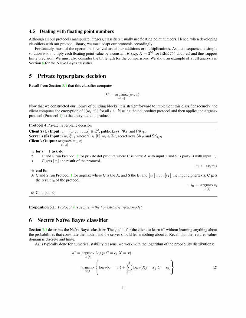
4.5 Dealing with floating point numbersAlthough all our protocols manipulate integers, classifiers usually use floating point numbers. Hence, when developingclassifiers with our protocol library, we must adapt our protocols accordingly.

Fortunately, most of the operations involved are either additions or multiplications. As a consequence, a simplesolution is to multiply each floating point value by a constant K (e.g. K = 252 for IEEE 754 doubles) and thus supportfinite precision. We must also consider the bit length for the comparisons. We show an example of a full analysis inSection 6 for the Naïve Bayes classifier.

5 Private hyperplane decisionRecall from Section 3.1 that this classifier computes

k∗ = argmaxi∈[k]

〈wi, x〉.

Now that we constructed our library of building blocks, it is straightforward to implement this classifier securely: theclient computes the encryption of J〈wi, x〉K for all i ∈ [k] using the dot product protocol and then applies the argmaxprotocol (Protocol 1) to the encrypted dot products.

Protocol 4 Private hyperplane decisionClient’s (C) Input: x = (x1, . . . , xd) ∈ Zd, public keys PKP and PKQRServer’s (S) Input: {wi}ki=1 where ∀i ∈ [k], wi ∈ Zn, secret keys SKP and SKQRClient’s Output: argmax

i∈[k]

〈wi, x〉

1: for i = 1 to k do2: C and S run Protocol 3 for private dot product where C is party A with input x and S is party B with input wi.3: C gets JviK the result of the protocol.

. vi ← 〈x,wi〉4: end for5: C and S run Protocol 1 for argmax where C is the A, and S the B, and Jv1K, . . . , JvkK the input ciphertexts. C gets

the result i0 of the protocol.. i0 ← argmax

i∈[k]

vi

6: C outputs i0

Proposition 5.1. Protocol 4 is secure in the honest-but-curious model.

6 Secure Naïve Bayes classifierSection 3.1 describes the Naïve Bayes classifier. The goal is for the client to learn k∗ without learning anything aboutthe probabilities that constitute the model, and the server should learn nothing about x. Recall that the features valuesdomain is discrete and finite.

As is typically done for numerical stability reasons, we work with the logarithm of the probability distributions:

k∗ = argmaxi∈[k]

log p(C = ci|X = x)

= argmaxi∈[k]

log p(C = ci) +

d∑j=1

log p(Xj = xj |C = ci)

(2)

11

6.1 Preparing the modelSince the Paillier encryption scheme works with integers, we convert each log of a probability from above to an integerby multiplying it with a large number K (recall that the plaintext space of Paillier is large ≈ 21024 thus allowing for alarge K), thus still maintaining high accuracy. The issues due to using integers for bayesian classification have beenpreviously studied in [TRMP12], even though their setting was even more restricting than ours. However, they use asimilar idea to ours: shifting the probabilities logarithms and use fixed point representation.

As the only operations used in the classification step are additions and comparisons (cf. Equation (2)), we can justmultiply the conditional probabilities p(xj |ci) by a constant K so to get integers everywhere, while keeping the sameclassification result.

For example, if we are able to compute the conditional probabilities using IEEE 754 double precision floating pointnumbers, with 52 bits of precision, then we can represent every probability p as

p = m · 2e

where m binary representation is (m)2 = 1.d and d is a 52 bits integer. Hence we have 1 ≤ m < 2 and we can rewritem as

m =m′

252with m′ ∈ N ∩ [252, 253)

We are using this representation to find a constant K such that K · vi ∈ N for all i. As seen before, we can write thevi’s as

vi = m′i · 2ei−52

Let e∗ = mini ei, and δi = ei − e∗ ≥ 0. Then,

vi = m′i · 2δi · 2e∗−52

So let K = 252−e∗ . We have K · vi = m′i · 2δi ∈ N. An important thing to notice is that the vi’s can be very largeintegers (due to δi), and this might cause overflows errors. However, remember that we are doing all this to storelogarithms of probabilities in Paillier cyphertexts, and as Paillier plaintext space is very large (more than 1024 bits inour setting) and δi’s remain small3. Also notice that this shifting procedure can be done without any loss of precision aswe can directly work with the bit representation of the floating points numbers.

Finally, we must also ensure that we do not overflow Paillier’s message space when doing all the operations(homomorphic additions, comparisons, . . . ). If – as before – d is the number of features, the maximum number of bitswhen doing the computations will be lmax = d+ 1 + (52 + δ∗) where δ∗ = max δi: we have to add the probabilitiesfor the d features and the probability of the class label (the d+ 1 term), and each probability is encoded using (52 + δ∗)bits. Hence, the value l used for the comparison protocols must be chosen larger than lmax.

Hence, we must ensure that log2N > lmax + 1 + λ where λ is the security parameter and N is the modulusfor Paillier’s cryptosystem plaintext space (cf. Section 4.1.2). This condition is easily fulfilled as, for a good level ofsecurity, we have to take log2N ≥ 1024 and we usually take λ ≈ 100.

Let Dj be the domain of possible values of xj (the j-th attribute of the feature vector x). The server prepares kd+ 1tables as part of the model, where K is computed as described just before:• One table for the priors on the classes P : P (i) = dK log p(C = ci)e.• One table per feature j per class i, Ti,j : Ti,j(v) ≈ dK log p(Xj = v|C = ci)e, for all v ∈ Dj .

The tables remain small: P has one entry by category i.e. k entries total, and T has one entry by category and featurevalue i.e. k · D entries where D =

∑ |Dj |. In our examples, this represents less than 3600 entries. Moreover, thispreparation step can be done once and for all at server startup, and is hence amortized.

3If the biggest δi is 10, the ratio between the smallest and the biggest probability is of order 2210

= 21024 ...

12

6.2 ProtocolLet us begin with some intuition. The server encrypts each entry in these tables with Paillier and gives the resultingencryption (the encrypted model) to the client. For every class ci, the client uses Paillier’s additive homomorphism tocompute JpiK = JP (i)K

∏dj=1JTi,j(xj)K. Finally, the client runs the argmax protocol, Protocol 1, to get argmax pi. For

completeness, the protocol is shown in Protocol 5.

Protocol 5 Naïve Bayes ClassifierClient’s (C) Input: x = (x1, . . . , xd) ∈ Zd, public key PKP , secret key SKQRServer’s (S) Input: The secret key SKP , public key PKQR and probability tables {log p(C = ci)}1≤i≤k and{{log p(Xj = v|C = ci)}v∈Dj

}1≤j≤d,1≤i≤k

Client’s Output: i0 such that p(x, ci0) is maximum

1: The server prepares the tables P and {Ti,j}1≤i≤k,1≤j≤d and encrypts their entries using Paillier.2: The server sends JP K and {JTi,jK}i,j to the client.3: For all 1 ≤ i ≤ k, the client computes JpiK = JP (i)K

∏dj=1JTi,j(xj)K.

4: The client runs the argmax protocol (Protocol 1) with the server and gets i0 = argmaxi pi5: C outputs i0

Proposition 6.1. Protocol 5 is secure in the honest-but-curious model.

Proof intuition. Given the security property of the argmax protocol, Protocol 1, and the semantic security of thePaillier cryptosystem, the security of this classifier follows trivially, by invoking a modular composition theorem.

Efficiency. Note that the tables P and {Ti,j}1≤i≤k,1≤j≤d can be prepared in advance. Hence the cost of constructingthe tables can be amortized over many uses. To compute the encrypted probabilities pi’s, the client runs d homomorphicoperations (here multiplications) for each i, hence doing kd modular multiplications. Then the parties run a singleargmax protocol i.e. k − 1 comparisons and O(k) homomorphic operations. Thus, compared to non-encryptedcomputation, the overhead comes only from the use of homomorphic encryption operations instead of plaintextoperations. Regarding the number of round trips, these are due to the argmax protocol: k − 1 runs of the comparisonprotocol and k − 1 additional roundtrips.

7 Private decision treesA private decision tree classifier allows the server to traverse a binary decision tree using the client’s input x such thatthe server does not learn the input x, and the client does not learn the structure of the tree and the thresholds at eachnode. A challenge is that, in particular, the client should not learn the path in the tree that corresponds to x – the positionof the path in the tree and the length of the path leaks information about the model. The outcome of the classificationdoes not necessarily leak the path in the tree

The idea is to express the decision tree as a polynomial P whose output is the result of the classification, the classpredicted for x. Then, the server and the client privately compute inputs to this polynomial based on x and the thresholdswi. Finally, the server evaluates the polynomial P privately.

7.1 Polynomial form of a decision treeConsider that each node of the tree has a boolean variable associated to it. The value of the boolean at a node is 1 if, oninput x, one should follow the right branch, and 0 otherwise. For example, denote the boolean variable at the root of thetree by b1. The value of b1 is 1 if x1 ≤ w1 (recall Figure 2), and 0 otherwise.

We construct a polynomial P that, on input all these boolean variables and the value of each class at a leafnode, outputs the class predicted for x. The idea is that P is a sum of terms, where each term (say t) corresponds

13

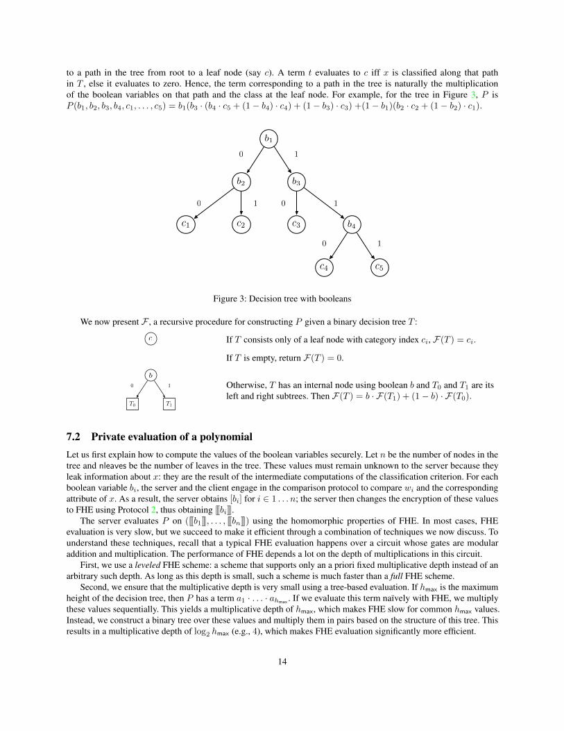
to a path in the tree from root to a leaf node (say c). A term t evaluates to c iff x is classified along that pathin T , else it evaluates to zero. Hence, the term corresponding to a path in the tree is naturally the multiplicationof the boolean variables on that path and the class at the leaf node. For example, for the tree in Figure 3, P isP (b1, b2, b3, b4, c1, . . . , c5) = b1(b3 · (b4 · c5 + (1− b4) · c4) + (1− b3) · c3) +(1− b1)(b2 · c2 + (1− b2) · c1).

b1

b2

c1 c2

b3

c3 b4

c4 c5

0 1

0 1

1

1

0

0

Figure 3: Decision tree with booleans

We now present F , a recursive procedure for constructing P given a binary decision tree T :

c If T consists only of a leaf node with category index ci, F(T ) = ci.

If T is empty, return F(T ) = 0.

T1T0

b

0 1 Otherwise, T has an internal node using boolean b and T0 and T1 are itsleft and right subtrees. Then F(T ) = b · F(T1) + (1− b) · F(T0).

7.2 Private evaluation of a polynomialLet us first explain how to compute the values of the boolean variables securely. Let n be the number of nodes in thetree and nleaves be the number of leaves in the tree. These values must remain unknown to the server because theyleak information about x: they are the result of the intermediate computations of the classification criterion. For eachboolean variable bi, the server and the client engage in the comparison protocol to compare wi and the correspondingattribute of x. As a result, the server obtains [bi] for i ∈ 1 . . . n; the server then changes the encryption of these valuesto FHE using Protocol 2, thus obtaining [JbiK].

The server evaluates P on ([Jb1K], . . . , [JbnK]) using the homomorphic properties of FHE. In most cases, FHEevaluation is very slow, but we succeed to make it efficient through a combination of techniques we now discuss. Tounderstand these techniques, recall that a typical FHE evaluation happens over a circuit whose gates are modularaddition and multiplication. The performance of FHE depends a lot on the depth of multiplications in this circuit.

First, we use a leveled FHE scheme: a scheme that supports only an a priori fixed multiplicative depth instead of anarbitrary such depth. As long as this depth is small, such a scheme is much faster than a full FHE scheme.

Second, we ensure that the multiplicative depth is very small using a tree-based evaluation. If hmax is the maximumheight of the decision tree, then P has a term a1 · . . . · ahmax . If we evaluate this term naïvely with FHE, we multiplythese values sequentially. This yields a multiplicative depth of hmax, which makes FHE slow for common hmax values.Instead, we construct a binary tree over these values and multiply them in pairs based on the structure of this tree. Thisresults in a multiplicative depth of log2 hmax (e.g., 4), which makes FHE evaluation significantly more efficient.

14

Finally, we use F2 as the plaintext space and SIMD slots for parallelism. FHE schemes are significantly faster whenthe values encrypted are bits (namely, in F2); however, P contains classes (e.g., c1) which are usually more than a bitin length. To enable computing P over F2, we represent each class in binary. Let l = dlog2 ke (k is the number ofclasses) be the number of bits needed to represent a class. We evaluate P l times, once for each of the l bits of a class.Concretely, the j-th evaluation of P takes as input b1, . . . , bn and for each leaf node ci, its j-th bit cij . The result isP (b1, . . . , bn, c1j , c2j , . . . , cnleavesj), which represents the j-th bit of the outcome class. Hence, we need to run the FHEevaluation l times.

To avoid this factor of l, the idea is to use a nice feature of FHE called SIMD slots (as described in [SV11]): theseallow encrypting multiple bits in a single ciphertext such that any operation applied to the ciphertext gets applied inparallel to each of the bits. Hence, for each class cj , the server creates an FHE ciphertext [Jcj0, . . . , cjl−1K]. For eachnode bi, it creates an FHE ciphertext [Jbi, . . . , biK] by simply repeating the bi value in each slot. Then, the server runsone FHE evaluation of P over all these ciphertexts and obtains [Jco0, . . . , col−1K] where co is the outcome class. Hence,instead of l FHE evaluations, the server runs the evaluation only once. This results in a performance improvement oflog k, a factor of 2 and more in our experiments. We were able to apply SIMD slots parallelism due to the fortunate factthat the same polynomial P had to be computed for each slot.

Finally, evaluating the decision tree is done using 2n FHE multiplications and 2n FHE additions where n is thenumber of criteria. The evaluation circuit has multiplication depth dlog2(n) + 1e.

7.3 Formal descriptionProtocol 6 describes the resulting protocol.

Protocol 6 Decision Tree ClassifierClient’s (C) Input: x = (x1, . . . , xn) ∈ Zn, secret keys SKQR,SKFHEServer’s (S) Input: The public keys PKQR,PKFHE , the model as a decision tree, including the n thresholds {wi}ni=1.Client’s Output: The value of the leaf of the decision tree associated with the inputs b1, . . . , bn.

1: S produces an n-variate polynomial P as described in section 7.1.2: S and C interact in the comparison protocol, so that S obtains [bi] for i ∈ [1 . . . n] by comparing wi to the

corresponding attribute of x.3: Using Protocol 2, S changes the encryption from QR to FHE and obtains [Jb1K], . . . , [JbnK].4: To evaluate P , S encrypts the bits of each category ci using FHE and SIMD slots, obtaining

[Jci1, . . . , cilK]. S uses SIMD slots to compute homomorphically [JP (b1, . . . , bn, c10, . . . , cnleaves0), . . . ,P (b1, . . . , bn, c1l−1, . . . , cnleavesl−1)K]. It rerandomizes the resulting ciphertext using FHE’s rerandomizationfunction, and sends the result to the client.

5: C decrypts the result as the bit vector (v0, . . . , vl−1) and outputs∑l−1i=0 vi · 2i.

Proposition 7.1. Protocol 6 is secure in the honest-but-curious model.

Proof intuition. The proof is in Appendix C, but we give some intuition here. During the comparison protocol, theserver only learns encrypted bits, so it learns nothing about x. During FHE evaluation, it similarly learns nothing aboutthe input due to the security of FHE. The client does not learn the structure of the tree because the server performs theevaluation of the polynomial. Similarly, the client does not learn the bits at the nodes in the tree because of the securityof the comparison protocol.

The interactions between the client and the server are due to the comparisons almost exclusively: the decision treeevaluation does not need any interaction but sending the encrypted result of the evaluation.

15

bool Linear_Classifier_Client::run(){

exchange_keys();

// values_ is a vector of integers// compute the dot productmpz_class v = compute_dot_product(values_);mpz_class w = 1; // encryption of 0

// compare the dot product with 0return enc_comparison(v, w, bit_size_, false);

}

void Linear_Classifier_Server_session::run_session()

{exchange_keys();

// enc_model_ is the encrypted model vector// compute the dot producthelp_compute_dot_product(enc_model_, true);

// help the client to get// the sign of the dot producthelp_enc_comparison(bit_size_, false);

}

Figure 4: Implementation example: a linear classifier

Bit size A Computation B Computation Total Time Communication Interactions10 14.11 ms 8.39 ms 105.5 ms 4.60 kB 320 18.29 ms 14.1 ms 117.5 ms 8.82 kB 332 22.9 ms 18.8 ms 122.6 ms 13.89 kB 364 34.7 ms 32.6 ms 134.5 ms 27.38 kB 3

Table 3: Comparison with unencrypted input protocols evaluation.

8 Combining classifiers with AdaBoostAdaBoost is a technique introduced in [FS97]. The idea is to combine a set of weak classifiers hi(x) : Rd 7→ {−1,+1}to obtain a better classifier. The AdaBoost algorithm chooses t scalars {αi}ti=1 and constructs a strong classifier as:

H(x) = sign

(t∑i=1

αihi(x)

)

If each of the hi(·)’s is an instance of a classifier supported by our protocols, then given the scalars αi, we can easilyand securely evaluate H(x) by simply composing our building blocks. First, we run the secure protocols for each ofhi, except that the server keeps the intermediate result, the outcome of hi(x), encrypted using one of our comparisonprotocols (Rows 2 or 4 of Table 2). Second, if necessary, we convert them to Paillier’s encryption scheme with Protocol 2,and combine these intermediate results using Paillier’s additive homomorphic property as in the dot product protocolProtocol 3. Finally, we run the comparison over encrypted data algorithm to compare the result so far with zero, so thatthe client gets the final result.

9 ImplementationWe have implemented the protocols and the classifiers in C++ using GMP4, Boost, Google’s Protocol Buffers5, andHELib [Hal13] for the FHE implementation.

The code is written in a modular way: all the elementary protocols defined in Section 4 can be used as black boxeswith minimal developer effort. Thus, writing secure classifiers comes down to invoking the right API calls to theprotocols. For example, for the linear classifier, the client simply calls a key exchange protocol to setup the variouskeys, followed by the dot product protocol, and then the comparison of encrypted data protocol to output the result, asshown in Figure 4.

4http://gmplib.org/5https://code.google.com/p/protobuf/

16

Protocol Bit sizeComputation

Total Time Communication InteractionsParty A Party B

Comparison 64 45.34 ms 43.78 ms 190.9 ms 27.91 kB 6Reversed Comp. 64 48.78 ms 42.49 ms 195.7 ms 27.91 kB 6

Table 4: Comparison with encrypted input protocols evaluation.

Party A Computation Party B Computation Total Time Communication Interactions30.80 ms 255.3 ms 360.7 ms 420.1 kB 2

Table 5: Change encryption scheme protocol evaluation.

10 EvaluationTo evaluate our work, we answer the following questions: (i) can our building blocks be used to construct otherclassifiers in a modular way (Section 10.1), (ii) what is the performance overhead of our building blocks (Section 10.3),and (iii) what is the performance overhead of our classifiers (Section 10.4)?

10.1 Using our building blocks libraryHere we demonstrate that our building blocks library can be used to build other classifiers modularly and that it isa useful contribution by itself. We will construct a multiplexer and a face detector. A face detection algorithm overencrypted data already exists [AB06, AB07], so our construction here is not the first such construction, but it serves asa proof of functionality for our library.

10.1.1 Building a multiplexer classifier

A multiplexer is the following generalized comparison function:

fα,β(a, b) =

{α if a > b

β otherwise

We can express fα,β as a linear combination of the bit d = (a ≤ b):

fα,β(d) = d · β + (1− d) · α = α+ d · (β − α).

To implement this classifier privately, we compute JdK by comparing a and b, keeping the result encrypted with QR,and then changing the encryption scheme (cf. Section 4.3) to Paillier.

Then, using Paillier’s homomorphism and knowledge of α and β, we can compute an encryption of fα,β(d):

Jfα,β(d)K = JαK · JdKβ−α.

10.1.2 Viola and Jones face detection

The Viola and Jones face detection algorithm [VJ01] is a particular case of an AdaBoost classifier. Denote by X animage represented as an integer vector and x a particular detection window (a subset of X’s coefficients). The strongclassifier H for this particular detection window is

H(x) = sign

(t∑i=1

αihi(x)

)

where the ht are weak classifiers of the form hi(x) = sign (〈x, yi〉 − θi) .

17

Data set Model sizeComputation Time per protocol Total

Comm. InteractionsClient Server Compare Dot product running time

Breast cancer (2) 30 46.4 ms 43.8 ms 194 ms 9.67 ms 204 ms 35.84 kB 7Credit (3) 47 55.5 ms 43.8 ms 194 ms 23.6 ms 217 ms 40.19 kB 7

(a) Linear Classifier. Time per protocol includes communication.

Data setSpecs. Computation Time per protocol Total

Comm. InteractionsC F Client Server Prob. Comp. Argmax running time

Breast Cancer (1) 2 9 150 ms 104 ms 82.9 ms 396 ms 479 ms 72.47 kB 14Nursery (5) 5 9 537 ms 368 ms 82.8 ms 1332 ms 1415 ms 150.7 kB 42

Audiology (4) 24 70 1652 ms 1664 ms 431 ms 3379 ms 3810 ms 1911 kB 166

(b) Naïve Bayes Classifier. C is the number of classes and F is the number of features. The Prob. Comp. column corresponds to thecomputation of the probabilities p(ci|x) (cf. Section 6). Time per protocol includes communication.

Data setTree Specs. Computation Time per protocol FHE

Comm. InteractionsN D Client Server Compare ES Change Eval. Decrypt

Nursery (5) 4 4 1579 ms 798 ms 446 ms 1639 ms 239 ms 33.51 ms 2639 kB 30ECG (6) 6 4 2297 ms 1723 ms 1410 ms 7406 ms 899 ms 35.1 ms 3555 kB 44

(c) Decision Tree Classifier. ES change indicates the time to run the protocol for changing encryption schemes. N is the number ofnodes of the tree and D is its depth. Time per protocol includes communication.

Table 6: Classifiers evaluation.

In our setting, Alice owns the image and Bob the classifier (e.g. the vectors {yi} and the scalars {θi} and {αi}).Neither of them wants to disclose their input to the other party. Thanks to our building blocks, Alice can run Bob’sclassifier on her image without her learning anything about the parameters and Bob learning any information about herimage.

The weak classifiers can be seen as multiplexers; with the above notation, we have ht(x) = f1,−1(〈x, yt〉 − θt).Using the elements of Section 10.1.1, we can easily compute the encrypted evaluation of every one of these weak

classifiers under Paillier, and then, as described in Section 8, compute the encryption of H(x).

10.2 Performance evaluation setupOur performance evaluations were run using two desktop computers each with identical configuration: two Intel Corei7 (64 bit) processors for a total 4 cores running at 2.66 GHz and 8 GB RAM. Since the machines were on the samenetwork, we inflated the roundtrip time for a packet to be 40 ms to mimic real network latency. We used 1024-bitcryptographic keys, and chose the statistical security parameter λ to be 100. When using HELib, we use 80 bits ofsecurity, which corresponds to a 1024-bit asymmetric key.

10.3 Building blocks performanceWe examine performance in terms of computation time at the client and server, communication bandwidth, and alsonumber of interactions (round trips). We can see that all these protocols are efficient, with a runtime on the order ofmilliseconds.

10.3.1 Comparison protocols

Comparison with unencrypted input. Table 3 gives the running time of the comparison protocol with unencryptedinput for various input size.

18

Comparison with encrypted input. Table 4 presents the performance of the comparison with encrypted inputsprotocols.

10.3.2 argmax

Figure 5 presents the running times and the communication overhead of the argmax of encrypted data protocol (cf.Section 4.2). The input integers were 64 bit integers.

0

1000

2000

3000

4000

5000

6000

7000

4 5 6 7 8 9 10 11 12 13 14 15 16 17 18 19 20 25 30 35 50

Tim

e (m

s)

Elements

Party AParty B

CommunicationTree

Figure 5: Argmax of encrypted data protocol evaluation. The bars represent the execution of the protocol when the comparisons areexecuted one after each other, linearly. The line represents the execution when comparisons are executed in parallel, tree-wise.

10.3.3 Consequences of the latency on performances

It is worth noticing that for most blocks, most of the running time is spend communicating: the network’s latency has ahuge influence on the performances of the protocols (running time almost linear in the latency for some protocols). Toimprove the performances of a classifier implemented with our blocks, we might want to run several instances of somebuilding blocks in parallel. This is actually what we did with the tree-based implementation of the argmax protocol,greatly improving the performances of the protocol (cf. Figure 5).

10.4 Classifier performanceHere we evaluate each of the classifiers described in Sections 5–7. The models are trained non-privately usingscikit-learn6. We used the following datasets from the UCI machine learning repository [BL13]:1. the Wisconsin Diagnostic Breast Cancer data set,2. the Wisconsin Breast Cancer (Original) data set, a simplified version of the previous dataset,3. Credit Approval data set,4. Audiology (Standardized) data set,5. Nursery data set, and

6http://scikit-learn.org

19

6. ECG (electrocardiogram) classification data from Barni et al. [BFK+09]These data sets are scenarios when we want to ensure privacy of the server’s model and client’s input.Based on the suitability of each classifier, we used data sets 2 and 3 to test the hyperplane decision classifier, sets 1,

4 and 5 for the Naïve Bayes classifier, and sets 5 and 6 for the decision tree classifier.Table 6 shows the performance results. Our classifiers run in at most a few seconds, which we believe to be practical

for sensitive applications. Note that even if the datasets become very large, the size of the model stays the same – thedataset size only affects the training phase which happens on unencrypted data before one uses our classifiers. Hence,the cost of our classification will be the same even for very large data sets.

For the decision tree classifier, we compared our construction to Barni et al. [BFK+09] on the ECG dataset (byturning their branching program into a decision tree). Their performance is 2609 ms7 for the client and 6260 ms for theserver with communication cost of 112.2KB. Even though their evaluation does not consider the communication delays,we are still more than three times as fast for the server and faster for the client.

10.5 Comparison to generic two-party toolsA set of generic secure two- or multi-party computation tools have been developed, such as TASTY [HKS+10] andFairplay [MNPS04, BDNP08]. These support general functions, which include our classifiers.

However, they are prohibitively slow for our specific setting. Our efficiency comes from specializing to classificationfunctionality. To demonstrate their performance, we attempted to evaluate the Naïve Bayes classifier with these. Weused FairplayMP to generate the circuit for this classifier and then TASTY to run the private computation on the circuitthus obtained. We tried to run the smallest Naïve Bayes instance, the Nursery dataset from our evaluation, which hasonly 3 possible values for each feature, but we ran out of memory during the circuit generation phase on a powerfulmachine with 256GB of RAM.

Hence, we had to reduce the classification problem to only 3 classes (versus 5). Then, the circuit generation tookmore than 2 hours with FairplayMP, and the time to run the classification with TASTY was 413196 msec (with nonetwork delay), which is ≈ 500 times slower than our performance (on the non-reduced classification problem with 5classes). Thus, our specialized protocols improve performance by orders of magnitude.

11 ConclusionIn this paper, we constructed three major privacy-preserving classifiers as well as provided a library of building blocksthat enables constructing other classifiers. We demonstrated the efficiency of our classifiers and library on real datasets.

AcknowledgmentWe thank Thijs Veugen, Thomas Schneider, and the anonymous reviewers for their helpful comments.

7In Barni et al. [BFK+09], the evaluation was run over two 3GHz computers directly connected via Gigabit Ethernet. We scaled the given resultsby 3

2.3to get a better comparison basis.

20

References[AB06] Shai Avidan and Moshe Butman. Blind vision. In Computer Vision–ECCV 2006, pages 1–13. 2006.

[AB07] Shai Avidan and Moshe Butman. Efficient methods for privacy preserving face detection. In Advances inNeural Information Processing Systems, page 57, 2007.

[AD01] Mikhail J Atallah and Wenliang Du. Secure multi-party computational geometry. In Algorithms and DataStructures, pages 165–179. 2001.

[BDMN05] Avrim Blum, Cynthia Dwork, Frank McSherry, and Kobbi Nissim. Practical privacy: the sulq framework.In Proceedings of the twenty-fourth ACM SIGMOD-SIGACT-SIGART symposium on Principles of databasesystems, pages 128–138, 2005.

[BDNP08] Assaf Ben-David, Noam Nisan, and Benny Pinkas. Fairplaymp: A system for secure multi-partycomputation. In CCS, pages 17–21, 2008.

[BFK+09] Mauro Barni, Pierluigi Failla, Vladimir Kolesnikov, Riccardo Lazzeretti, Ahmad-Reza Sadeghi, andThomas Schneider. Secure evaluation of private linear branching programs with medical applications. InComputer Security (ESORICS), pages 424–439. 2009.

[BFL+09] Mauro Barni, Pierluigi Failla, Riccardo Lazzeretti, Annika Paus, A-R Sadeghi, Thomas Schneider, andVladimir Kolesnikov. Efficient privacy-preserving classification of ecg signals. In Information Forensicsand Security, 2009. WIFS 2009. First IEEE International Workshop on, pages 91–95, 2009.

[BFL+11] Mauro Barni, Pierluigi Failla, Riccardo Lazzeretti, Ahmad-Reza Sadeghi, and Thomas Schneider. Privacy-preserving ECG classification with branching programs and neural networks. IEEE Transactions onInformation Forensics and Security (TIFS), 6(2):452–468, June 2011.

[BGV12] Zvika Brakerski, Craig Gentry, and Vinod Vaikuntanathan. (Leveled) fully homomorphic encryptionwithout bootstrapping. In ITCS, pages 309–325, 2012.

[BHKR13] Mihir Bellare, Viet Tung Hoang, Sriram Keelveedhi, and Phillip Rogaway. Efficient garbling from afixed-key blockcipher. In IEEE SP, pages 478–492, 2013.

[BL13] K. Bache and M. Lichman. UCI machine learning repository, 2013.

[BLN13] Joppe W. Bos, Kristin Lauter, and Michael Naehrig. Private predictive analysis on encrypted medical data.In Microsoft Tech Report 200652, 2013.

[BN06] Christopher M Bishop and Nasser M Nasrabadi. Pattern recognition and machine learning. In Journal ofElectronic Imaging, volume 1, 2006.

[Can98] Ran Canetti. Security and composition of multi-party cryptographic protocols. JOURNAL OFCRYPTOLOGY, 13:2000, 1998.

[CMS11] Kamalika Chaudhuri, Claire Monteleoni, and Anand D. Sarwate. Differentially private empirical riskminimization. J. Mach. Learn. Res., 12, 2011.

[DGK07] Ivan Damgård, Martin Geisler, and Mikkel Krøigaard. Efficient and secure comparison for on-line auctions.In Information Security and Privacy, pages 416–430, 2007.

[DGK09] Ivan Damgard, Martin Geisler, and Mikkel Kroigard. A correction to efficient and secure comparison foron-line auctions. 1(4):323–324, 2009.

[DHC04] Wenliang Du, Yunghsiang S Han, and Shigang Chen. Privacy-preserving multivariate statistical analysis:Linear regression and classification. In Proceedings of the 4th SIAM International Conference on DataMining, volume 233, 2004.

21

[EFG+09] Zekeriya Erkin, Martin Franz, Jorge Guajardo, Stefan Katzenbeisser, Inald Lagendijk, and Tomas Toft.Privacy-preserving face recognition. In Privacy Enhancing Technologies, pages 235–253, 2009.

[FS97] Yoav Freund and Robert E Schapire. A decision-theoretic generalization of on-line learning and anapplication to boosting. Journal of computer and system sciences, (1):119–139, 1997.

[Gen09] Craig Gentry. Fully homomorphic encryption using ideal lattices. In STOC, pages 169–178, 2009.

[GLLM04] Bart Goethals, Sven Laur, Helger Lipmaa, and Taneli Mielikäinen. On private scalar product computationfor privacy-preserving data mining. In Information Security and Cryptology (ICISC), pages 104–120.2004.

[GLN12] Thore Graepel, Kristin Lauter, and Michael Naehrig. ML confidential: Machine learning on encrypteddata. In Information Security and Cryptology (ICISC), pages 1–21. 2012.

[GM82] Shafi Goldwasser and Silvio Micali. Probabilistic encryption and how to play mental poker keeping secretall partial information. In STOC, pages 365–377. ACM, 1982.

[GMW87] O. Goldreich, S. Micali, and A. Wigderson. How to play any mental game. In STOC, pages 218–229,1987.

[Gol04] Oded Goldreich. Foundations of Cryptography - Basic Applications. Cambridge University Press, 2004.

[Hal13] Shai Halevi. Helib - an implementation of homomorphic encryption. https://github.com/shaih/HElib,2013.

[HKS+10] Wilko Henecka, Stefan Kögl, Ahmad-Reza Sadeghi, Thomas Schneider, and Immo Wehrenberg. Tasty:Tool for automating secure two-party computations. In CCS, pages 451–462, 2010.

[IPS08] Yuval Ishai, Manoj Prabhakaran, and Amit Sahai. Founding cryptography on oblivious transfer – efficiently.In Advances in Cryptology – CRYPTO 2008, volume 5157, pages 572–591. 2008.

[Kil05] Eike Kiltz. Unconditionally secure constant round multi-party computation for equality, comparison, bitsand exponentiation. IACR Cryptology ePrint Archive, page 66, 2005.

[KSS09] Vladimir Kolesnikov, Ahmad-Reza Sadeghi, and Thomas Schneider. How to combine homomorphicencryption and garbled circuits - improved circuits and computing the minimum distance efficiently. In 1stInternational Workshop on Signal Processing in the EncryptEd Domain (SPEED’09), 2009.

[KSS13] Vladimir Kolesnikov, Ahmad-Reza Sadeghi, and Thomas Schneider. A systematic approach to practicallyefficient general two-party secure function evaluation protocols and their modular design. In Journal ofComputer Security, 2013.

[LLM06] Sven Laur, Helger Lipmaa, and Taneli Mielikäinen. Cryptographically private support vector machines. InProceedings of the 12th ACM SIGKDD international conference on Knowledge discovery and data mining,pages 618–624. ACM, 2006.

[LP00] Yehuda Lindell and Benny Pinkas. Privacy preserving data mining. In Advances in Cryptology (CRYPTO),pages 36–54, 2000.

[LP07] Yehuda Lindell and Benny Pinkas. An efficient protocol for secure two-party computation in the presenceof malicious adversaries. In Advances in Cryptology (EUROCRYPT), volume 4515, pages 52–78. 2007.

[LP08] Yehuda Lindell and Benny Pinkas. Secure multi-party computation for privacy-preserving data mining. InCrypto ePrint Archive, 2008.

[LP09] Yehuda Lindell and Benny Pinkas. A proof of security of Yao’s protocol for two-party computation. J.Cryptol., 22:161–188, April 2009.

22

[LT05] Hsiao-Ying Lin and Wen-Guey Tzeng. An efficient solution to the millionaires’ problem based onhomomorphic encryption. In Applied Cryptography and Network Security, pages 456–466, 2005.

[MNPS04] Dahlia Malkhi, Noam Nisan, Benny Pinkas, and Yaron Sella. Fairplay-secure two-party computationsystem. In USENIX Security Symposium, pages 287–302, 2004.

[NP01] Moni Naor and Benny Pinkas. Efficient oblivious transfer protocols. In Proceedings of the twelfth annualACM-SIAM symposium on Discrete algorithms, pages 448–457, 2001.

[Pai99] Pascal Paillier. Public-key cryptosystems based on composite degree residuosity classes. In EUROCRYPT,pages 223–238, 1999.

[RR07] Ali Rahimi and Benjamin Recht. Random features for large-scale kernel machines. In NIPS, 2007.

[SG11] Anima Singh and John Guttag. Cardiovascular risk stratification using non-symmetric entropy-basedclassification trees. In NIPS workshop on personalized medicine, 2011.

[SG13] Anima Singh and John Guttag. Leveraging hierarchical structure in diagnostic codes for predicting incidentheart failure. In ICML workshop on role of machine learning in transforming healthcare, 2013.

[SSW09] Ahmad-Reza Sadeghi, Thomas Schneider, and Immo Wehrenberg. Efficient privacy-preserving facerecognition. In Information, Security and Cryptology (ICISC), pages 229–244. 2009.

[SV11] Nigel P. Smart and Frederik Vercauteren. Fully homomorphic SIMD operations. Cryptology ePrintArchive, Report 2011/133, 2011.

[TRMP12] Sebastian Tschiatschek, Peter Reinprecht, Manfred Mücke, and Franz Pernkopf. Bayesian networkclassifiers with reduced precision parameters. In Machine Learning and Knowledge Discovery inDatabases, pages 74–89. 2012.

[Veu11] Thijs Veugen. Comparing encrypted data. http://msp.ewi.tudelft.nl/sites/default/files/Comparingencrypteddata.pdf, 2011.

[VJ01] Paul Viola and Michael Jones. Rapid object detection using a boosted cascade of simple features. In IEEEComputer Vision and Pattern Recognition (CVPR), volume 1, pages I–511, 2001.

[VKC08] Jaideep Vaidya, Murat Kantarcıoglu, and Chris Clifton. Privacy-preserving naive bayes classification. TheInternational Journal on Very Large Data Bases, 17(4):879–898, 2008.

[WGH12] Jenna Wiens, John Guttag, and Eric Horvitz. Learning evolving patient risk processes for c. diffcolonization. In ICML, 2012.

[WY04] Rebecca Wright and Zhiqiang Yang. Privacy-preserving bayesian network structure computation ondistributed heterogeneous data. In Proceedings of the tenth ACM SIGKDD international conference onKnowledge discovery and data mining, pages 713–718, 2004.

[Yao82] Andrew C. Yao. Protocols for secure computations. In FOCS, pages 160–164, 1982.

[ZW05] Zhiqiang Yang1 Sheng Zhong and Rebecca N Wright. Privacy-preserving classification of customer datawithout loss of accuracy. In SIAM International Conference on Data Mining (SDM), 2005.

23

A Comparison protocols

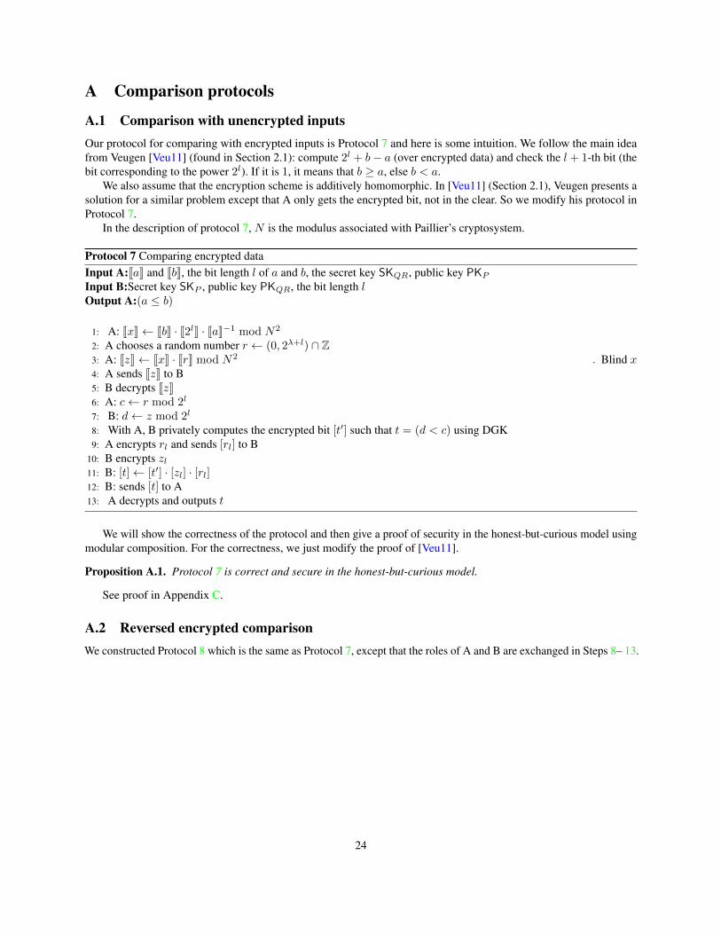
A.1 Comparison with unencrypted inputsOur protocol for comparing with encrypted inputs is Protocol 7 and here is some intuition. We follow the main ideafrom Veugen [Veu11] (found in Section 2.1): compute 2l + b− a (over encrypted data) and check the l + 1-th bit (thebit corresponding to the power 2l). If it is 1, it means that b ≥ a, else b < a.

We also assume that the encryption scheme is additively homomorphic. In [Veu11] (Section 2.1), Veugen presents asolution for a similar problem except that A only gets the encrypted bit, not in the clear. So we modify his protocol inProtocol 7.

In the description of protocol 7, N is the modulus associated with Paillier’s cryptosystem.

Protocol 7 Comparing encrypted dataInput A:JaK and JbK, the bit length l of a and b, the secret key SKQR, public key PKPInput B:Secret key SKP , public key PKQR, the bit length lOutput A:(a ≤ b)

1: A: JxK← JbK · J2lK · JaK−1 mod N2

2: A chooses a random number r ← (0, 2λ+l) ∩ Z3: A: JzK← JxK · JrK mod N2 . Blind x4: A sends JzK to B5: B decrypts JzK6: A: c← r mod 2l

7: B: d← z mod 2l

8: With A, B privately computes the encrypted bit [t′] such that t = (d < c) using DGK9: A encrypts rl and sends [rl] to B

10: B encrypts zl11: B: [t]← [t′] · [zl] · [rl]12: B: sends [t] to A13: A decrypts and outputs t

We will show the correctness of the protocol and then give a proof of security in the honest-but-curious model usingmodular composition. For the correctness, we just modify the proof of [Veu11].

Proposition A.1. Protocol 7 is correct and secure in the honest-but-curious model.

See proof in Appendix C.

A.2 Reversed encrypted comparisonWe constructed Protocol 8 which is the same as Protocol 7, except that the roles of A and B are exchanged in Steps 8– 13.

24

Proposition A.2. Protocol 8 is secure in the honest-but-curious model.

The proof is in Appendix C.

Protocol 8 Reversed comparing encrypted dataInput A:JaK and JbK, public keys PKQR and PKPInput B:Secret keys SKP and SKQROutput B:(a ≤ b)

Run Steps 1– 7 of Protocol 7.8: With B, A privately computes the encrypted bit [t′] such that t′ = (d < c) using DGK9: B encrypts zl and sends [zl] to A

10: A encrypts rl11: A: [t]← [t′] · [zl] · [rl]12: A: sends [t] to B13: B decrypts and outputs t

B Preliminaries for proofs

B.1 Secure two-party computation frameworkAll our protocols are two-party protocols, which we label as party A and party B. In order to show that they do privatecomputations, we work in the honest-but-curious (semi-honest) model as described in [Gol04].

Let f = (fA, fB) be a (probabilistic) polynomial function and Π a protocol computing f . A and B want tocompute f(a, b) where a is A’s input and b is B’s input, using Π and with the security parameter λ. The view ofparty A during the execution of Π is the tuple VA(λ, a, b) = (1λ; a; rA;mA

1 , . . . ,mAt ) where r is A’s random tape

and mA1 , . . . ,m

At are the messages received by A. We define the view of B similarly. We also define the outputs of

parties A and B for the execution of Π on input (a.b) as OutputΠA(λ, a, b) and OutputΠB(λ, a, b), and the global outputas OutputΠ(λ, a, b) = (OutputΠA(λ, a, b),OutputΠB(λ, a, b)).

To ensure security, we have to show that whatever A can compute from its interactions with B can be computedfrom its input and output, which leads us to the following security definition.

Definition B.1. The two-party protocol Π securely computes the function f if there exists two probabilistic polynomialtime algorithms SA and SB such that for every possible input a, b of f ,

{SA(1λ,a, fA(a, b)), f(a, b)} ≡c{VA(λ, a, b),OutputΠ(λ, a, b)}

and

{SB(1λ,a, fB(a, b)), f(a, b)} ≡c{VB(λ, a, b),OutputΠ(λ, a, b)}

where ≡c means computational indistinguishability against probabilistic polynomial time adversaries with negligibleadvantage in the security parameter λ.

To simplify the notation (and the proofs), hereinafter we omit the security parameter. As we mostly considerdeterministic functions f , we can simplify the distributions we want to show being indistinguishable (see [Gol04]):when f is deterministic, to prove the security of Π that computes f , we only have to show that

SA(a, fA(a, b)) ≡c VA(a, b)

SB(b, fB(a, b)) ≡c VB(a, b)

Unless written explicitly, we will always prove security using this simplified definition.

25

B.2 Modular Sequential CompositionIn order to ease the proofs of security, we use sequential modular composition, as defined in [Can98]. The idea isthat the parties run a protocol Π and use calls to an ideal functionality f in Π (e.g. A and B compute f privately bysending their inputs to a trusted third party and receiving the result). If we can show that Π respects privacy in thehonest-but-curious model and if we have a protocol ρ that privately computes f in the same model, then we can replacethe ideal calls for f by the execution of ρ in Π; the new protocol, denoted Πρ is then secure in the honest-but-curiousmodel.

We call hybrid model with ideal access to f1, . . . , fm or (f1, . . . , fm)-hybrid model the semi-honest modelaugmented with an incorruptible trusted party T for evaluating functionalities f1, . . . , fm. The parties run a protocol Πthat contain calls to T for the evaluation of one of f1, . . . , fm. For each call, each party sends its input and wait untilthe trusted party sends the output back. We emphasize on the fact that the parties must not communicate until receivingT ’s output (we consider only sequential composition). Ideal calls to the trusted party can be done several times, evenfor the same function, but each call is independent: T does not maintain state between two calls.

Let Π be a two-party protocol in the (f1, . . . , fm)-hybrid model. Let ρ1, . . . , ρm be real protocols (i.e. protocols inthe semi-honest model) computing f1, . . . , fm and define Πρ1,...,ρm as follows. All ideals calls of Π to the trusted partyfor fi is replaced by a real execution of ρi: if party Pj has to compute fi with input xj , Pj halts, starts an execution ofρi with the other parties, gets the result βj when ρi concludes, and continues as if βj was received from T .

Theorem B.2. [Can98] (Theorem 5) restated as in [LP08] (Theorem 3) – Let f1, . . . , fm be two-party probabilisticpolynomial time functionalities and ρ1, . . . , ρm protocols that compute respectively f1, . . . , fm in the presence ofsemi-honest adversaries.

Let g be a two-party probabilistic polynomial time functionality and Π a protocol that securely computes g in the(f1, . . . , fm)-hybrid model in the presence of semi-honest adversaries.

Then Πρ1,...,ρm securely computes g in the presence of semi-honest adversaries.

B.3 Cryptographic assumptionsAssumption 1. (Quadratic Residuosity Assumption – from [GM82]) Let N = p× q be the product of two distinct oddprimes p and q. Let QRN be the set of quadratic residues modulo N and QNRN be the set of quadratic non residues(i.e. x ∈ QNRN if x is not a square modulo N and its Jacobi symbol is 1).{(N,QRN ) : |N | = λ} and {(N,QNRN ) : |N | = λ} are computationally indistinguishable with respect to

probabilistic polynomial time algorithms.

Assumption 2. (Decisional Composite Residuosity Assumption – from [Pai99]) Let N = p × q, |N | = λ be theproduct of two distinct odd primes p and q. A number z is said to be a N -th residue modulo N2 if there exists a numbery ∈ ZN2

z = yN mod N2

N -th residues are computationally indistinguishable from non N -th residues with respect to probabilistic polynomialtime algorithms.

For further explanations about the last assumption, used for the FHE scheme, we refer the reader to [BGV12].

Assumption 3. (RLWE) For security parameter λ, let f(x) = xd + 1 where d is a power of 2. Let q ≥ 2 be an integer.Let R = Z[x]/(f(x)) and let Rq = R/qR. Let χ be a distribution over R. The RLWEd,q,χ problem is to distinguishbetween two distributions: In the first distribution, one samples (ai, bi) uniformly from R2

q . In the second distribution,one first draws s← Rq uniformly and then samples (ai, bi) ∈ R2

q by sampling ai ← Rq uniformly, ei ← χ, and settingbi = ai.s+ ei.

The RLWEd,q,χ assumption is that the RLWEd,q,χ problem is infeasible.

26

C Proofs

C.1 Comparison protocols

Proof of Proposition A.1 . Correctness As a and b are l bits integers, x = 2l + b−a is a l+ 1 bits integer and its mostsignificant bit (the l + 1-th bit) is 1 iff a ≤ b. What protocol 7 actually does is computing this bit. The computations aredone over encrypted data, using Paillier’s encryption scheme. In the rest of the proof, we will do as if the data were notencrypted under Paillier. The correctness will hold as long as we do not experience carry-overs modulo N . In particular,this implies that l+ 1 + λ < log2N . For operations over bits using QR, we don’t have this problem as we are operatingon F2.

Again, since x is a l+ 1 bit number, its most significant bit is x÷ 2l where ÷ denotes the integer division. We havex = 2l(x÷ 2l) + (x mod 2l) where 0 ≤ (x mod 2l) < 2l. As z = x+ r,

z = 2l(z ÷ 2l) + (z mod 2l)

= 2l((x÷ 2l) + (r ÷ 2l)) + ((x mod 2l) + (r mod 2l))

Hence, z ÷ 2l = x÷ 2l + r ÷ 2l if (x mod 2l) + (r mod 2l) < 2l and z ÷ 2l = (x÷ 2l) + (r ÷ 2l) + 1 otherwise.More generally, z ÷ 2l = (x÷ 2l) + (r ÷ 2l) + t′ where t′ = 0⇔ (x mod 2l) + (r mod 2l) < 2l.

We can also notice that, if t′ = 0, z mod 2l = (x mod 2l) + (r mod 2l) and z mod 2l = (x mod 2l) + (r mod2l)− 2l otherwise. As a consequence,

t′ = 0⇔ z mod 2l = (x mod 2l) + (r mod 2l)

⇔ z mod 2l ≥ (r mod 2l)

In the end, as x÷ 2l is either 0 or 1, we can compute everything modulo 2

x÷ 2l = (z ÷ 2l)− (r ÷ 2l)− t′ mod 2

= zl ⊕ rl ⊕ t′

Security We suppose that the encrypted bit [t′] is ideally computed (using calls to a trusted party in the hybrid model).We show that the protocol is secure in this model and conclude using the sequential modular composition theorem.

A’s view is VA = (JaK, JbK, l, SKQR,PKP ; r, coins; [t]) where SKQR is the secret key for the QR cryptosystem,PKP is the public key for Paillier’s cryptosystem, and coins are the random coins used for the encryptions of 2l, r andrl. Given (JaK, JbK, l, SKQR,PKP , a ≤ b), we build the simulator SA:1. Compute [t] an encryption of the bit (a ≤ b) under QR.2. Pick r ← (0, 2λ+l) ∩ Z.

3. Let coins be random coins for two Paillier encryptions and one QR encryption.

4. Output (JaK, JbK, l, SKQR,PKP ; r, coins; [t])

The distributions VA(JaK, JbK, l, SKQR,PKQR,SKP ,PKP ) and SA(JaK, JbK,SKQR,PKP , a ≤ b) are exactly the samebecause the randomness is taken from the same distribution in both cases, and the QR cyphertext encrypts the same bit.

B’s view is VB = (PKQR,SKP , l, JzK; coins; [t′], [rl]) where coins are the random coins used for the encryption ofzl. The simulator SB(PKQR,SKP , l) runs as follows:1. Pick z ← (0, 2λ+l) ∩ Z.2. Encrypt z under Paillier: JzK.3. Generate [t′] and [rl], two encryptions of random bits under QR

4. Let coins be random coins for one QR encryption.

5. Output (PKQR,SKP , l, JzK; coins; [t′], [rl])

27

The random tapes coins and coins are generated in the exact same manner and independently from any otherparameter, so

(PKQR,SKP , JzK; coins; [t′][rl])

= (PKQR,SKP , JzK; coins; [t′][rl])

Recall that z = x + r mod N where x is an l bits integer and r is an l + λ bits integer. But as we chosel + 1 + λ < log2N , we have z = x+ r. The distribution of z is statistically indistinguishable from the distribution ofz (the distributions are distinguishable with an advantage of 2−λ at most).

We also directly have that (SKP , JzK) ≡s (SKP , JzK) and as a consequence, as the distribution of z and z isindependent from t′ and rl,

(PKQR,SKP , JzK; coins; [t′], [rl])

≡s (PKQR,SKP , JzK; coins; [t′], [rl])

By semantic security of QR,

(PKQR,SKP , l, JzK; coins; [t′], [rl])

≡c (PKQR,SKP , l, JzK; coins; [t′], [rl])

and

SB(PKQR,SKP , l)

≡c VB(JaK, JbK, l, SKQR,PKQR,SKP ,PKP )

We conclude the proof of security using modular sequential composition. We replace the ideal calls for computingthe encrypted bit [t′] by the provable secure DGK protocol and invoke Theorem B.2 to prove security in the semi-honestmodel.

Proof of Proposition A.2. The proof of security is similar to the one of Proposition A.1. Again we first suppose that [t′]is ideally computed (hybrid model).

A’s view is VA = (JaK, JbK, l,PKQR,PKP ; r, coins; [t′], [zl]) where PKQR is the public key for the QR cryptosystem,PKP is the public key for Paillier’s cryptosystem and coins is the random tape used for the Paillier encryptions of r and2l, and the QR encryption of rl.

Given (JaK, JbK,PKQR,PKP ), we build the simulator SA:1. Pick r ← (0, 2λ+l) ∩ Z.2. Generate [t′] and [zl], two encryptions of random bits under QR

3. Let coins be random coins for two Paillier encryptions and one QR encryption.

4. Output (JaK, JbK, l,PKQR,PKP ; r, coins; [zl])

For both cases (A’s view and the simulator SA), r and r are taken from the same uniform distribution over(0, 2λ+l) ∩ Z, and coins and coins are random tapes of the same length, so

SA(JaK, JbK,PKQR,PKP )

= (JaK, JbK, l,PKQR,PKP ; r, coins; [zl])

By semantic security of the QR cryptosystem, we conclude with the computational indistinguishability of SA and VAdistributions:

SA(JaK, JbK,PKQR,PKP )

= (JaK, JbK, l,PKQR,PKP ; r, coins; [zl])

≡c (JaK, JbK, l,PKQR,PKP ; r, coins; [zl])

= VA(JaK, JbK, l, SKQR,PKQR,SKP ,PKP )

28

B’s view is VB = (SKQR,SKP , JzK, [t]; coins) where SKQR is the secret key for the QR cryptosystem, SKP isthe secret key for Paillier’s cryptosystem, and coins are the random coins necessary for the QR encryption of zl. Thesimulator SB(SKQR,SKP , a ≤ b) runs as follows:1. Compute [t] an encryption of the bit (a ≤ b) under QR.2. Pick z ← (0, 2λ+l) ∩ Z.3. Encrypt z under Paillier: JzK.

4. Let coins be random coins for one QR encryption.

5. Output (SKQR,SKP , l, JzK, [t]; coins)

Once again, the distributions of coins and coins are identical:

(SKQR,SKP , l, JzK, [t]; coins)

= (SKQR,SKP , l, JzK, [t]; coins)

Recall that z = x + r where x is an l bits integer and r is an l + λ bits integer. The distribution of z is statisticallyindistinguishable from the distribution of z. We also directly have that (SKP , JzK) ≡s (SKP , JzK) and as a consequence,as the distribution of z and z is independent from t′,

(SKQR,SKP , l, JzK, [t]; coins)

≡s (SKQR,SKP , l, JzK, [t]; coins)

Moreover, by construction, (SKQR, [t]) = (SKQR, [a < b]) and

(SKQR,SKP , l, JzK, [t]; coins)= (SKQR,SKP , l, JzK, [a < v]; coins).

Finally, we have

SB(SKQR,SKP , a ≤ b)≡s VB(JaK, JbK, l, SKQR,PKQR,SKP ,PKP ).

Again, we conclude the proof of security using modular sequential composition. We replace the ideal calls forcomputing the encrypted bit [t′] by the provable secure DGK protocol and invoke Theorem B.2 to prove security in thesemi-honest model.

C.1.1 Argmax

Proof of Proposition 4.1. Correctness To prove correctness, we have to show that the following invariant holds: atthe end of the loop for iteration i, m is the maximum of {aπ(j)}1≤j≤i and aπ(i0) = m.

If this holds, at the end of the loop iterations aπ(i0) is the maximum of {aπ(j)}1≤j≤k = {aj}1≤j≤k, hencei0 = argmaxj aπ(j) and π−1(i0) = argmaxj aj .

At initialization (line 4), the invariant trivially holds as the family {aπ(j)}1≤j≤i contains only one element.Suppose the property is true for iteration i− 1. Let us distinguish two cases:

• If bi is true (i.e. m ≤ aπ(i)), max{aπ(j)}1≤j≤i−1 ≤ aπ(i), as the invariant holds for the previous iteration, and thenmax{aπ(j)}1≤j≤i = aπ(i).Then i0 is set to i, vi = a′i and bi = 1. As a consequence, m is set by A to

vi + (bi − 1).ri − bi.si = a′i − si = aπ(i)

We have clearly that aπ(i0) = aπ(i) = m and m = max{aπ(j)}1≤j≤i, the invariant holds at the end of the i-thiteration in this case.

29

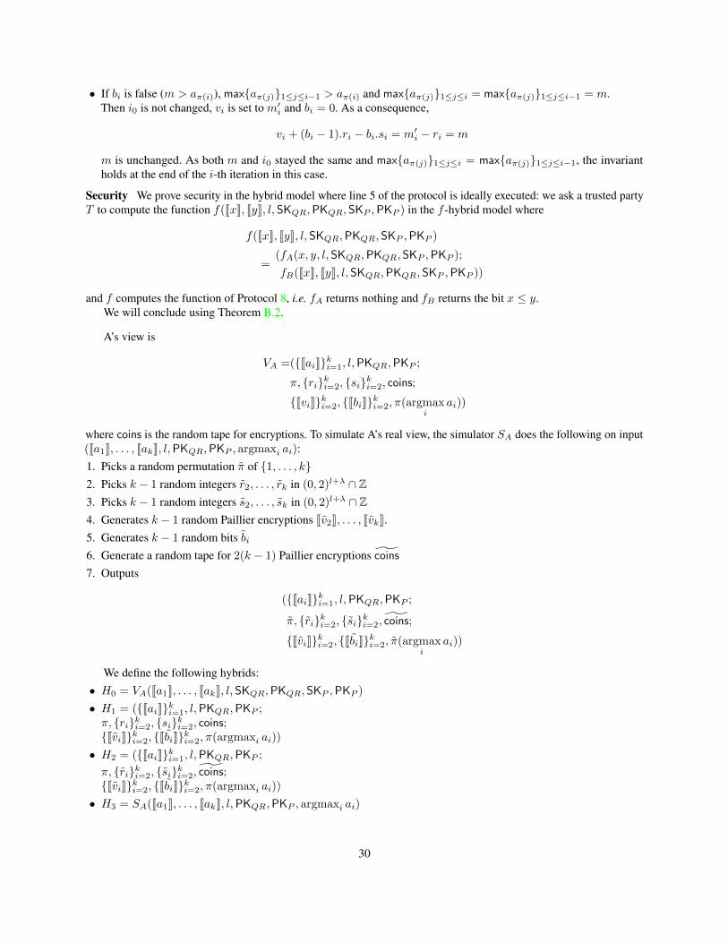
• If bi is false (m > aπ(i)), max{aπ(j)}1≤j≤i−1 > aπ(i) and max{aπ(j)}1≤j≤i = max{aπ(j)}1≤j≤i−1 = m.Then i0 is not changed, vi is set to m′i and bi = 0. As a consequence,

vi + (bi − 1).ri − bi.si = m′i − ri = m

m is unchanged. As both m and i0 stayed the same and max{aπ(j)}1≤j≤i = max{aπ(j)}1≤j≤i−1, the invariantholds at the end of the i-th iteration in this case.

Security We prove security in the hybrid model where line 5 of the protocol is ideally executed: we ask a trusted partyT to compute the function f(JxK, JyK, l, SKQR,PKQR,SKP ,PKP ) in the f -hybrid model where

f(JxK, JyK, l, SKQR,PKQR,SKP ,PKP )

=(fA(x, y, l,SKQR,PKQR,SKP ,PKP );

fB(JxK, JyK, l, SKQR,PKQR,SKP ,PKP ))

and f computes the function of Protocol 8, i.e. fA returns nothing and fB returns the bit x ≤ y.We will conclude using Theorem B.2.

A’s view is

VA =({JaiK}ki=1, l,PKQR,PKP ;

π, {ri}ki=2, {si}ki=2, coins;

{JviK}ki=2, {JbiK}ki=2, π(argmaxi

ai))

where coins is the random tape for encryptions. To simulate A’s real view, the simulator SA does the following on input(Ja1K, . . . , JakK, l,PKQR,PKP , argmaxi ai):1. Picks a random permutation π of {1, . . . , k}2. Picks k − 1 random integers r2, . . . , rk in (0, 2)l+λ ∩ Z3. Picks k − 1 random integers s2, . . . , sk in (0, 2)l+λ ∩ Z4. Generates k − 1 random Paillier encryptions Jv2K, . . . , JvkK.5. Generates k − 1 random bits bi6. Generate a random tape for 2(k − 1) Paillier encryptions coins7. Outputs

({JaiK}ki=1, l,PKQR,PKP ;

π, {ri}ki=2, {si}ki=2, coins;

{JviK}ki=2, {JbiK}ki=2, π(argmaxi

ai))

We define the following hybrids:• H0 = VA(Ja1K, . . . , JakK, l, SKQR,PKQR,SKP ,PKP )

• H1 = ({JaiK}ki=1, l,PKQR,PKP ;π, {ri}ki=2, {si}ki=2, coins;{JviK}ki=2, {JbiK}ki=2, π(argmaxi ai))

• H2 = ({JaiK}ki=1, l,PKQR,PKP ;

π, {ri}ki=2, {si}ki=2, coins;{JviK}ki=2, {JbiK}ki=2, π(argmaxi ai))

• H3 = SA(Ja1K, . . . , JakK, l,PKQR,PKP , argmaxi ai)

30

By semantic security of Paillier’s cryptosystem,

({JaiK}ki=1, l,PKQR,PKP ;π, {ri}ki=2, {si}ki=2;

{JviK}ki=2, {JbiK}ki=2, π(argmaxi

ai))

≡c({JaiK}ki=1, l,PKQR,PKP ;π, {ri}ki=2, {si}ki=2;

{JviK}ki=2, {JbiK}ki=2π(argmaxi

ai))

and H0 ≡c H1 as π(argmaxi ai) = i0Given that the ri, si and coins are generated according to the same distribution as ri, si (uniform over (0, 2)l+λ ∩Z)

and coins (random tape for 2(k − 1) Paillier encryptions), and that they are completely independent from the vi or π,the hybrids H1 and H2 are equal.

Similarly, the distribution of (π, π(argmaxi ai)) and(π, π(argmaxi ai)) are exactly the same. As π and π are independent from the other parameters, we also haveH2 = H3.

Hence, we showed that

VA({JaiK}ki=1, l, SKQR,PKQR,SKP ,PKP )

≡c SA({JaiK}ki=1, l,PKQR,PKP , argmaxi

ai).

B’s view is

VB = (SKP ,SKQR, l; coins; {bi}ki=2, {Jm′iK}ki=2, {Ja′iK}ki=2)

where coins are the random coins for k − 1 Paillier cyphertext refresh. The simulator SB(SKP ,SKQR, l) runs asfollows:1. Generates a random permutation π of {1, . . . , k}2. Set JaiK = JiK3. Run the protocol with the JaiK as input data, π as the permutation, and same parameters otherwise. Let

(SKP ,SKQR, l; coins; {bi}ki=2, {Jm′iK}ki=2, {Ja′iK}ki=2) be B’s view of this run.4. Outputs

(SKP ,SKQR, l; coins; {bi}ki=2, {Jm′iK}ki=2, {Ja′iK}ki=2)

Let p : {ai}1≤i≤k 7→ {1, . . . , k} be the function that associates ai to its rank among the ai (in ascendent order).Let us fix the permutation π for a while and define the following hybrids:0. H0 = VB({JaiK}ki=1, l, SKQR,PKQR,SKP ,PKP )

1. H1 = VB({Jp(a1)K}ki=1, l, SKQR,PKQR,SKP ,PKP )

We will show that these hybrids are statistically equal for every permutation π.As p(.) is a map that does not change the order of the ai, we have that for all i, j, ai ≤ aj ⇔ p(ai) ≤ p(aj). As

a consequence, for a given permutation π, the bits bi do not change if we replace the ai by p(ai). Similarly, the waythe a′i and m′i are generated for H0 and H1 is the same: blinding by adding random noise from (0, 2λ+l ∩ Z). Thus,H0 ≡s H1.

Now, we want to show that H1 ≡s SB(SKP ,SKQR, l) - we do not fix π anymore. Let π0 be the permutation suchthat p(ai) = π0(i). We can then rewrite H1 as

H1 = VB(Jπ0(1)K, . . . , Jπ0(k)K, l, SKQR,PKQR,SKP ,PKP )

As π and π ◦ π0 are statistically indistinguishable, we have H1 ≡s SB(SKP ,SKQR, l): recall that SB’s output is theview of B when the protocol is run with the set {ai = i} as input set and π as the permutation. Hence

VB(Ja1K, . . . , JakK, l, SKQR,PKQR,SKP ,PKP )

≡s SB(SKP ,SKQR, l)

31

We conclude the proof of security using modular sequential composition. We replace the ideal calls for computingthe encrypted bits bi by the provable secure Protocol 8 and invoke Theorem B.2 to prove security in the semi-honestmodel.

C.2 Changing the encryption scheme

Proof of Proposition 4.2. In this protocol the computed function is probabilistic, and we have to show security accordingto the full definition (cf. section B.1). The function is f :

f(JcK1,PK1,PK2,SK1,SK2) = (JcK2, ∅)

For the sake of simplicity, we do not take into account the randomness used for the encryptions of r for A and c′ for B.As before, the distribution of these coins for one party is completely independent of the other elements to be taken inaccount in the simulations, so we just do not mention them in security proof.

A’s view is VA = (PK1,PK2, JcK1; r; Jc′K2). A’s output is JcK2. The simulator SA(PK1,PK2, JcK1) runs as follows:1. Picks uniformly at random r ←M and c′ ←M .2. Generates the encryption Jc′K2 of c′ under E2.3. Outputs (PK1,PK2, JcK1; r; Jc′K2).

r and r are taken from the same distribution, independently from any other parameter, so

{(PK1,PK2, JcK1; r; Jc′K2); f(JcK1,PK1,PK2,SK1,SK2)}= {(PK1,PK2, JcK1; r; Jc′K2); f(JcK1,PK1,PK2,SK1,SK2)}

(c′ depends on r but does not appear in the previous distributions). By semantic security of scheme E2 we have that

{(PK1,PK2, JcK1; r; Jc′K2); f(JcK1,PK1,PK2,SK1,SK2)}≡c {(PK1,PK2, JcK1; r; Jc′K2); JcK2}

and so

{SA(JcK1,PK1,PK2), f(JcK1,PK1,PK2,SK1,SK2)}≡c {VA(JcK1,PK1,PK2,SK1,SK2),Output(JcK1,PK1,PK2,SK1,SK2)}

B’s view is VB = (SK1,SK2; Jc+ rK1). We build a simulator SB(SK1,SK2):1. Picks a random c←M .2. Encrypt c under E1.3. Outputs (SK1,SK2, JcK1).

Again, the distribution of c and c + r are identical, so the real distribution {(SK1,SK2; Jc + rK1); JcK2} and theideal distribution {(SK1,SK2; JrK1); f(JcK1,PK1,PK2,SK1,SK2)} are statistically indistinguishable.

C.3 Computing dot productsProof of Proposition 4.3. As B does not receive any message, its view only consists in its input and its random tapeused for the encryptions. Hence the simulator SB simply generate random coins and

SB(y,SKP ) = (y,SKP ; coins) = VB(x, y, SKP ,PKP ).

where rand are the random coins.

A’s view is VA = (x,PKP ; rA; Jy1K, . . . , JynK). On input (x,PKP , JvK), the simulator SA does the following:

32

1. Generates n encryptions of 0 using Paillier: c1, . . . , cn.

2. Generates the random coins necessary for a Paillier re-randomization and put them in coins.

3. Outputs (x,PKP ; coins; c1, . . . , cn).

coins and coins come from the same distribution, independently from other parameters. Thus,

{(x,PKP ; coins; c1, . . . , cn); J〈x, y〉K}= {(x,PKP ; coins; c1, . . . , cn); J〈x, y〉K}

and by semantic security of Paillier,

{(x,PKP ; coins; c1, . . . , cn); J〈x, y〉K}≡c {(x,PKP ; coins; Jy1K, . . . , JynK); JvK}

i.e., when f is f(x, y,SKP ,PKP ) = (J〈x, y〉K, ∅)

{SA(x,PKP , JvK); f(x, y, SKP ,PKP )}≡c {VA(x, y,SKP ,PKP );Output(x, y, SKP ,PKP )}

C.4 Classifiers

Hyperplane decision

Proof of Proposition 5.1. The client’s view is

VC = (PKP ,PKQR, x; {JviK}ki=1, i0).

The simulator SC , on input (PKP ,SKQR, x, k∗) where k∗ = argmax

i∈[k]

〈wi, x〉 does the following:

1. Generate k random Paillier encryptions JviK2. Output (PKP ,SKQR, x; {JvK}ki=1, k

∗)

As the index i0 that the client receives is its output, and as Paillier’s cryptosystem is semantically secure, thedistributions SC = (PKP ,SKQR, x; {JvK}ki=1, k

∗) and VC = (PKP ,SKQR, x; {JviK}ki=1, i0) are computationallyindistinguishable.

As the server views nothing but its inputs (the server does not receive any message in the hybrid model), we use forthe trivial simulator that just outputs its inputs for the proof of security.

As Protocols 1 and 3 are secure in the honest-but-curious model, we obtain the security of the hyperplane decisionprotocol using modular sequential composition (Theorem B.2).

Bayes classifier

Proof of Proposition 6.1. The client’s view is

VC = (PKP ,SKQR, x; JP K, {JTi,jK}, i0).

The simulator SC , on input (PKP ,SKQR, x, imax) where imax = argmaxj P(C = cj |X = x),

• generates tables of random Paillier encryptions JP K and {JTi,jK};• outputs (PKP ,SKQR, x; JP K, {JTi,jK}, imax).

33

As the integer i0 that the client receives is its output, and as Paillier’s cryptosystem is semantically secure,the distributions SC = (PKP ,SKQR, x; JP K, {JTi,jK}, imax) and VC = (PKP ,SKQR, x; JP K, {JTi,jK}, i0) arecomputationally indistinguishable.

Again, as the server views nothing but its inputs (the server does not receive any message in the hybrid model), weuse the trivial simulator that outputs its inputs and the random coins for the encryption for the proof of security.

As Protocol 1 is secure in the honest-but-curious model, we obtain the security of the hyperplane decision protocolusing modular sequential composition (Theorem B.2).

Decision tree

Proof of Proposition 7.1. The proof of security for the server is very easily obtained using modular sequentialcomposition of the comparison protocol and Protocol 2: in the hybrid model, the client receives nothing but theencrypted result.

For the client also the proof is trivial, using modular sequential composition and the semantical security of QR andof the FHE scheme: the encryptions of bits bi are computational indistinguishable from random bits whether they areencrypted under QR or the FHE scheme.

34