ma 5037: optimization methods and applications chapter 10

MA 5037: Optimization Methods and ApplicationsChapter 10: Optimality Conditions for LCPs

Suh-Yuh Yang (楊肅煜)

Department of Mathematics, National Central UniversityJhongli District, Taoyuan City 32001, Taiwan

[email protected]://www.math.ncu.edu.tw/∼syyang/

Suh-Yuh Yang (楊肅煜), Math. Dept., NCU, Taiwan MA 5037/Chapter 10: Optimality Conditions for LCPs – 1/24

Optimality conditions

One of the main drawbacks of the concept of stationarity is thatfor most feasible sets, it is rather difficult to validate whether thiscondition is satisfied or not, and it is even more difficult to use itin order to actually solve the underlying optimization problem.

Our main objective is to derive an equivalent optimality conditionthat is much easier to handle.

We will establish the so-called Karush-Kuhn-Tucker (KKT)conditions for the special case of linearly constrained problems(LCPs).


Strict separation theorem

Definition: Given S ⊆ Rn, a hyperplane H := {x ∈ Rn : a>x = b},where a ∈ Rn \ {0} and b ∈ R, is said to strictly separate a pointy 6∈ S from S if a>y > b and a>x ≤ b, ∀ x ∈ S.

NLO2014/9/17page 192�

��

�

��

��

192 Chapter 10. Optimality Conditions for Linearly Constrained Problems

S

{x : aT x=b}

y

Figure 10.1. Strict separation of point from a closed and convex set.

which is the same as(y− x)T x≤ (y− x)T x for all x ∈C .

Denote p= y− x �= 0 (since y /∈C ) and α= (y− x)T x. Then we have that pT x≤ α for allx ∈C . On the other hand,

pT y= (y− x)T y= (y− x)T (y− x)+ (y− x)T x= ‖y− x‖2+α > α,

and the result is established.

As was already mentioned, the latter separation theorem is extremely important sinceit is the basis for all optimality conditions. We begin by using it in order to prove an al-ternative theorem, which is known in the literature as Farkas’ lemma. We refer to it as analternative theorem since it essentially states that exactly one of two systems (“alterna-tives”) is feasible.

Lemma 10.2 (Farkas’ lemma). Let c ∈ �n and A ∈ �m×n . Then exactly one of thefollowing systems has a solution:

I. Ax≤ 0,cT x> 0.

II. AT y= c,y≥ 0.

Before proceeding to the proof of the lemma, let us begin with an illustration. Forthat, consider the following example:

A=�

1 5−1 2

�, c=

�−19

�,

Stating that system I is infeasible means that the system Ax ≤ 0 implies the inequalitycT x ≤ 0. Thus, the relevant question is whether the inequality −x1 + 9x2 ≤ 0 holdswhenever the two inequalities

x1+ 5x2 ≤ 0,−x1+ 2x2 ≤ 0

are satisfied. The answer to this question is affirmative. Indeed, we can see the implicationby noting that adding twice the second inequality to the first inequality yields the desiredinequality−x1+9x2 ≤ 0. Thus, the argument for showing the implication is that the row

Theorem: (strict separation theorem) Let C ⊆ Rn be a closed andconvex set, and let y 6∈ C. Then ∃ p ∈ Rn \ {0} and α ∈ R s.t.

p>y > α and p>x ≤ α, ∀ x ∈ C.Proof: By the second projection theorem, the vector x := PC(y) ∈ C satisfies

(y− x)>(x− x) ≤ 0 ∀ x ∈ C =⇒ (y− x)>x ≤ (y− x)>x ∀ x ∈ C.

Denote p = y− x 6= 0 and α = (y− x)>x. Then we have p>x ≤ α ∀ x ∈ C. Onthe other hand, p>y = (y− x)>y = (y− x)>(y− x) + (y− x)>x = ‖y− x‖2 + α.Thus, we have p>y > α, and the result is established. �


An alternative theorem: Farkas’ lemma

Farkas’ lemma: Let c ∈ Rn and A ∈ Rm×n. Then exactly one of thefollowing systems has a solution:(I) Ax ≤ 0, c>x > 0. (II) A>y = c, y ≥ 0.Example: Consider the following example

A =

[1 5−1 2

], c =

[−19

].

System (I) is infeasible since the system Ax ≤ 0 implies theinequality c>x ≤ 0. In practice,

x + 5y ≤ 0,−x + 2y ≤ 0.

Then eqn(1) + 2× eqn(2)⇒ −x + 9y ≤ 0, i.e., c>x ≤ 0. The rowvector c> can be written as a conic combination of the rows of A.In other words, c is a conic combination of the columns of A>:[

15

]+ 2

[−12

]=

[−19

]or[

1 −15 2

]︸︷︷︸

A>

[12

]=

[−19

]︸︷︷︸

c

.


Farkas’ lemma: second formulation

Let c ∈ Rn and A ∈ Rm×n. Then the following two claims are equivalent:(A) The implication Ax ≤ 0⇒ c>x ≤ 0 holds true.(B) ∃ y ∈ Rm

+ such that A>y = c.Proof: (B)⇒ (A): Assume that system (B) is feasible. Let Ax ≤ 0 for some x ∈ Rn. Theny>Ax ≤ 0. Since c> = y>A, we have c>x ≤ 0.

(A)⇒ (B): Suppose in contradiction that system (B) is infeasible. Consider thefollowing closed and convex set S := {x ∈ Rn : x = A>y for some y ∈ Rm

+}. (Theclosedness of S follows from Lemma 6.32). Then c 6∈ S. By the strict separationtheorem, ∃ p ∈ Rn \ {0} and α ∈ R s.t.

p>c > α and p>x ≤ α, ∀ x ∈ S.

Since 0 ∈ S, we can conclude that α ≥ 0 and also p>c > 0(⇒ c>p > 0). In addition,

p>x ≤ α, ∀ x ∈ S⇐⇒ p>A>y ≤ α, ∀ y ≥ 0⇐⇒ (Ap)>y ≤ α, ∀ y ≥ 0,

which implies Ap ≤ 0. We have thus arrived at a contradiction to the assumption thatthe implication (A) holds (using the vector p), and consequently (B) is satisfied. �


Gordan’s alternative theorem

Let A ∈ Rm×n. Then exactly one of the following two systems has asolution: (A) Ax < 0. (B) p 6= 0, A>p = 0, p ≥ 0.Proof: Assume that system (A) has a solution. Suppose in contradiction that (B) isfeasible. Then ∃ p 6= 0, A>p = 0, p ≥ 0. =⇒ x>A>p = 0 =⇒ (Ax)>p = 0. This isimpossible since Ax < 0 and 0 ≤ p 6= 0.

Now suppose that system (A) does not have a solution. Note that

Ax < 0 ⇐⇒ Ax + se ≤ 0, for some s > 0.

The latter system can be rewritten as

A[

xs

]≤ 0, c>

[xs

]> 0,

where A = [A e] and c = en+1. The infeasibility of (A) is thus equivalent to theinfeasibility of the system

Aw ≤ 0, c>w > 0, w ∈ Rn+1.

By Farkas’ lemma, ∃ z ∈ Rm+ s.t.[

A>

e>

]z = c =⇒ A>z = 0, e>z = 1.

Since e>z = 1, z 6= 0. We have shown the existence of 0 6= z =: p ∈ Rm+ s.t. A>z = 0. �


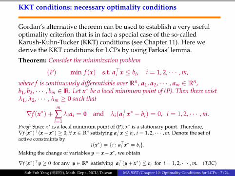
KKT conditions: necessary optimality conditions

Gordan’s alternative theorem can be used to establish a very usefuloptimality criterion that is in fact a special case of the so-calledKarush-Kuhn-Tucker (KKT) conditions (see Chapter 11). Here wederive the KKT conditions for LCPs by using Farkas’ lemma.

Theorem: Consider the minimization problem

(P) min f (x) s.t. a>i x ≤ bi, i = 1, 2, · · · , m,

where f is continuously differentiable over Rn, a1, a2, · · · , am ∈ Rn,b1, b2, · · · , bm ∈ R. Let x∗ be a local minimum point of (P). Then there existλ1, λ2, · · · , λm ≥ 0 such that

∇f (x∗) +m

∑i=1

λiai = 0 and λi(a>i x∗ − bi) = 0, i = 1, 2, · · · , m.

Proof: Since x∗ is a local minimum point of (P), x∗ is a stationary point. Therefore,∇f (x∗)>(x− x∗) ≥ 0, ∀ x ∈ Rn satisfying a>i x ≤ bi, i = 1, 2, · · · , m. Denote the set ofactive constraints by

I(x∗) = {i : a>i x∗ = bi}.Making the change of variables y = x− x∗, we obtain

∇f (x∗)>y ≥ 0 for any y ∈ Rn satisfying a>i (y + x∗) ≤ bi for i = 1, 2, · · · , m. (TBC)


KKT conditions: necessary optimality conditions (cont’d)

That is, we have

∇f (x∗)>y ≥ 0 for any y ∈ Rn satisfying a>i y ≤ 0, i ∈ I(x∗) & a>i y ≤ bi−a>i x∗, i 6∈ I(x∗). (?)

We will show that in fact the second set of inequalities in the latter system can beremoved, that is, that the following implication is valid:

If a>i y ≤ 0 for all i ∈ I(x∗) then ∇f (x∗)>y ≥ 0 (⇒ −∇f (x∗)>y ≤ 0).

Assume that y satisfies a>i y ≤ 0 for all i ∈ I(x∗).(1) Since bi − a>i x∗ > 0 for all i 6∈ I(x∗), it follows that there exists a small enough

α > 0 such that a>i (αy) ≤ bi − a>i x∗.(2) In addition, a>i (αy) ≤ 0 for all i ∈ I(x∗).

Therefore, from (?), we have ∇f (x∗)>(αy) ≥ 0 and hence that ∇f (x∗)>y ≥ 0. ByFarkas’ lemma (second formulation), ∃ λi ≥ 0, i ∈ I(x∗), such that

−∇f (x∗) = ∑i∈I(x∗)

λiai.

Defining λi = 0 for all i 6∈ I(x∗), we get that λi(a>i x∗ − bi) = 0 for all i = 1, 2, · · · , m and

∇f (x∗) +m

∑i=1

λiai = 0

as required. �


KKT conditions: sufficient optimality conditions

The KKT conditions are necessary conditions, but when f is convex,they are both necessary and sufficient global optimality conditions.


(P) min f (x) s.t. a>i x ≤ bi, i = 1, 2, · · · , m,

where f is a convex continuously differentiable function over Rn, a1, a2, · · · ,am ∈ Rn, b1, b2, · · · , bm ∈ R. Let x∗ be a feasible solution of (P). Then x∗ isan optimal solution of (P) if and only if ∃ λ1, λ2, · · · , λm ≥ 0 such that

∇f (x∗) +m

∑i=1

λiai = 0 and λi(a>i x∗ − bi) = 0, i = 1, 2, · · · , m. (?)

Note:

The nonnegative scalars λ1, λ2, · · · , λm in the KKT conditionsare called Lagrange multipliers, where λi is the multiplierassociated with the ith constraint a>i x ≤ bi.

The conditions λi(a>i x∗ − bi) = 0, i = 1, 2, · · · , m are known inthe literature as the complementary slackness conditions.


Proof of the sufficient optimality conditions

(⇒) It has been done in the previous theorem.(⇐) Assume that x∗ be a feasible solution of (P) satisfying (?). Let xbe any feasible solution of (P). Define the function

h(x) := f (x) +m

∑i=1

λi(a>i x− bi).

Then ∇h(x∗) = 0 and since h is convex, it follows that x∗ is aminimizer of h over Rn. From (?), we have

f (x∗) = f (x∗) +m

∑i=1

λi(a>i x∗ − bi) = h(x∗)

≤ h(x) = f (x) +m

∑i=1

λi(a>i x− bi) ≤ f (x).

We have thus proven that x∗ is a global optimal solution of (P). �


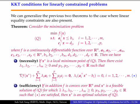
KKT conditions for linearly constrained problems

We can generalize the previous two theorems to the case where linearequality constraints are also present.


(Q)

min f (x)s.t. a>i x ≤ bi, i = 1, 2, · · · , m,

c>j x = dj, j = 1, 2, · · · , p,

where f is a continuously differentiable function over Rn, a1, a2, · · · , am,c1, c2, · · · , cp ∈ Rn, b1, b2, · · · , bm, d1, d2, · · · , dp ∈ R. Then we have

1 (necessity) If x∗ is a local minimum point of (Q). Then there existλ1, λ2, · · · , λm ≥ 0 and µ1, µ2, · · · , µp ∈ R such that

∇f (x∗)+m

∑i=1

λiai +p

∑j=1

µjcj = 0, λi(a>i x∗− bi) = 0, i = 1, 2, · · · , m. (?)

2 (sufficiency) If in addition f is convex over Rn and x∗ is a feasiblesolution of (Q) for which ∃ λ1, λ2, · · · , λm ≥ 0, µ1, µ2, · · · , µp ∈ R

such that (?) are satisfied, then x∗ is an optimal solution of (Q).


Proof of the KKT theorem

The proof is based on the simple observation that a linear equality constraint a>x = bcan be written as two inequality constraints, a>x ≤ b and −a>x ≤ −b.

(1) Consider the equivalent problem

(Q′)min f (x)s.t. a>i x ≤ bi, i = 1, 2, · · · , m,

c>j x ≤ dj, −c>j x ≤ −dj, j = 1, 2, · · · , p.

Since x∗ is an optimal solution of (Q’), it follows that there exist multipliersλ1, λ2, · · · , λm ≥ 0 and µ+

1 , µ−1 , µ+2 , µ−2 , · · · , µ+

p , µ−p ≥ 0 such that

∇f (x∗) +m

∑i=1

λiai +p

∑j=1

µ+j cj −

p

∑j=1

µ−j cj = 0, (?1)

λi(a>i x∗ − bi) = 0, i = 1, 2, · · · , m, (?2)

µ+j (c>j x∗ − dj) = 0, µ−j (−c>j x∗ + dj) = 0, j = 1, 2, · · · , p. (?3)

We thus obtain that (?) are satisfied with µj := µ+j − µ−j , j = 1, 2, · · · , p.

(2) Assume that x∗ satisfies (?). Then it also satisfies (?1), (?2) and (?3) withµ+

j = max{µj, 0}, µ−j = −min{µj, 0}. By the theorem on page 9, x∗ is an optimalsolution of (Q’) and thus also an optimal solution of (Q). �

Note: A feasible point x∗ is called a KKT point if there exist multipliersfor which (?) on page 11 are satisfied.


General nonlinear programming problems

The general setting of general nonlinear programming problems isgiven by

(NLP)min f (x)s.t. gi(x) ≤ 0, i = 1, 2, · · · , m,

hj(x) = 0, j = 1, 2, · · · , p,

where f , g1, · · · , gm, h1, · · · , hp are all continuously differentiablefunctions over Rn. The associated Lagrangian function takes the form

L(x, λ, µ) = f (x) +m

∑i=1

λigi(x) +p

∑j=1

µjhj(x).

In the linearly constrained case of problem (Q), the first condition in(?) on page 11 is the same as

∇xL(x∗, λ, µ) = ∇f (x∗) +m

∑i=1

λi∇gi(x) +p

∑j=1

µj∇hj(x) = 0.


The associated Lagrangian function of problem (Q)

Back to problem (Q), we define the matrices A and C and the vectorsb and d by

A =

a>1a>2...

a>m

, C =

c>1c>2...

c>p

, b =

b1b2...

bm

, d =

d1d2...

dp

,

then the constraints of problem (Q) can be written as

Ax ≤ b, Cx = d.

The Lagrangian can be also written as

L(x, λ, µ) = f (x) + λ>(Ax− b) + µ>(Cx− d),

and the first condition in (?) takes the form

∇xL(x∗, λ, µ) = ∇f (x∗) + A>λ + C>µ = 0.


Example 1

Consider the problem

min12(x2 + y2 + z2) s.t. x + y + z = 3.

Since the problem is convex, the KKT conditions are necessary andsufficient. The Lagrangian of the problem is

L(x, y, z, µ) =12(x2 + y2 + z2) + µ(x + y + z− 3).

The KKT conditions and the feasibility condition are

∂L∂x

= x + µ = 0,∂L∂y

= y + µ = 0,

∂L∂z

= z + µ = 0, x + y + z = 3.

We obtain x = y = z = 1 and µ = −1. The unique optimal solution ofthe problem is (x, y, z) = (1, 1, 1).


Example 2

Consider the problem

min x2 + 2y2 + 4xy s.t. x + y = 1, x ≥ 0, y ≥ 0.

The problem is nonconvex, since the matrix associated with the

quadratic objective function A =

[1 22 2

]is indefinite. Thus, the KKT

conditions are necessary optimality conditions. The Lagrangian ofthe problem is

L(x, y, µ, λ1, λ2) = x2 + 2y2 + 4xy + µ(x + y− 1)− λ1x− λ2y,

where λ1, λ2 ∈ R+, µ ∈ R. The KKT conditions with the feasibilityconditions are

∂L∂x

= 2x + 4y + µ− λ1 = 0,∂L∂y

= 4x + 4y + µ− λ2 = 0,

λ1x = 0, λ2y = 0, x + y = 1, x ≥ 0, y ≥ 0, λ1, λ2 ≥ 0.

Case 1: λ1 = λ2 = 0. In this case we obtain the three equations2x + 4y + µ = 0, 4x + 4y + µ = 0, x + y = 1,

whose solution is (x, y, µ) = (0, 1,−4). (x, y) = (0, 1) is a KKT point.Suh-Yuh Yang (楊肅煜), Math. Dept., NCU, Taiwan MA 5037/Chapter 10: Optimality Conditions for LCPs – 16/24

Example 2 (cont’d)

Case 2: λ1 > 0, λ2 > 0. By the complementary slackness conditions,we have x = y = 0, which contradicts the constraint x + y = 1.

Case 3: λ1 > 0, λ2 = 0. By the complementary slackness conditions,we have x = 0⇒ y = 1, which was already shown to be a KKT point.

Case 4: λ1 = 0, λ2 > 0. By the complementary slackness conditions,we have y = 0⇒ x = 1⇒

2 + µ = 0, 4 + µ− λ2 = 0 =⇒ µ = −2, λ2 = 2.

We thus obtain that (x, y) = (1, 0) is also a KKT point.

Since the problem consists of minimizing a continuous function overa compact set it follows by the Weierstrass theorem that it has aglobal optimal solution.

f (1, 0) = 1, f (0, 1) = 2.

Therefore, (x, y) = (1, 0) is the global optimal solution of the problem.


Orthogonal projection onto an affine space

Let C be the affine space C := {x ∈ Rn : Ax = b}, where A ∈ Rm×n

and b ∈ Rm. We assume that the rows of A are linearly independent.Given y ∈ Rn, the optimization problem is

min ‖x− y‖2 s.t. Ax = b.

This is a convex optimization problem, so the KKT conditions arenecessary and sufficient. The Lagrangian function is

L(x, λ) = ‖x− y‖2 + (2λ)>(Ax− b) (Note µ := 2λ)

= ‖x‖2 − 2(y−A>λ)>x− 2λ>b + ‖y‖2, λ ∈ Rm.

The KKT conditions are

2x− 2(y−A>λ) = 0, Ax = b

=⇒ x = y−A>λ =⇒ A(y−A>λ) = b

=⇒ AA>λ = Ay− b =⇒ λ = (AA>)−1(Ay− b)

AA> is nonsingular since the rows of A are linearly independent. Weobtain the optimal solution PC(y) = y−A>(AA>)−1(Ay− b).


Orthogonal projection onto hyperplanes

1 Consider the hyperplane H = {x ∈ Rn : a>x = b}, where0 6= a ∈ Rn and b ∈ R. Since a hyperplane is a spacial case of anaffine space, from the last example, we obtain

PH(y) = y− a(a>a)−1(a>y− b) = y− a>y− b‖a‖2 a.

2 (distance of a point from a hyperplane)Let H = {x ∈ Rn : a>x = b}, where 0 6= a ∈ Rn and b ∈ R. Then

d(y, H) = ‖y− PH(y)‖ = ‖y−(

y− a>y− b‖a‖2 a

)‖ = |a

>y− b|‖a‖ .


Orthogonal projection onto half-spaces

Let H− = {x ∈ Rn : a>x ≤ b}, where 0 6= a ∈ Rn and b ∈ R. Giveny ∈ Rn, the corresponding optimization problem is

minx‖x− y‖2 s.t. a>x ≤ b.

The Lagrangian of the problem is

L(x, λ) = ‖x− y‖2 + (2λ)(a>x− b), λ ≥ 0,

and the KKT conditions with the feasibility condition are

2(x− y) + 2λa = 0, λ(a>x− b) = 0, a>x ≤ b, λ ≥ 0.

NLO2014/9/17page 203�

��

�

��

��

10.3. Orthogonal Regression 203

�2 �1.5 �1 �0.5 0 0.5 1�1

�0.8

�0.6

�0.4

�0.2

0

0.2

0.4

0.6

0.81

y

H={ x: aTx ≤ b}*

PH(y)

Figure 10.2. A vector y and its orthogonal projection onto a half-space.

The first equation implies that

x=−Q−1(c+AT λ). (10.15)

Plugging this expression of x into the feasibility constraint we obtain

−AQ−1(c+AT λ) = b,

so thatλ=−(AQ−1AT )−1(b+AQ−1c). (10.16)

The optimal solution of the problem is given by (10.15) with λ as in (10.16).

10.3 Orthogonal RegressionAn interesting application to the formula for the distance between a point and a hyper-plane given in Lemma 10.12 is in the orthogonal regression problem, which we now recall.Consider the points a1, . . . ,am in �n . For a given 0 �= x ∈ �n and y ∈ �, we define thehyperplane

Hx,y :=�a ∈�n : xT a= y

.

In the orthogonal regression problem we seek to find a nonzero vector x ∈�n and y ∈�such that the sum of squared Euclidean distances between the points a1, . . . ,am to Hx,y isminimal; that is, the problem is given by

minx,y

+m∑

i=1

d (ai , Hx,y )2 : 0 �= x ∈�n , y ∈�

,. (10.17)

An illustration of the solution to the orthogonal regression problem is given in Figure10.3.

The optimal solution of the orthogonal regression problem is described in the nextresult whose proof strongly relies on the formula of the distance between a point and ahyperplane.

A vector y and its orthogonal projection onto a half-spaceSuh-Yuh Yang (楊肅煜), Math. Dept., NCU, Taiwan MA 5037/Chapter 10: Optimality Conditions for LCPs – 20/24

Orthogonal projection onto half-spaces (cont’d)

1 If λ = 0, then x = y and the KKT conditions are satisfied whena>y ≤ b, i.e., y ∈ H−. Thus, the optimal solution is PH−(y) = yif y ∈ H−.

2 Assume that λ > 0. By the complementary slackness conditionwe have a>x = b. Plugging the first equation x = y− λa intoa>x = b, we have

a>(y− λa) = b =⇒ λ =a>y− b‖a‖2 > 0, when a>y > b.

The optimal solution is

x = y− a>y− b‖a‖2 a.

3 To summarize, we have

PH−(y) =

{y, a>y ≤ b,

y− a>y−b‖a‖2 a a>y > b.


The orthogonal regression problem

Consider the points a1, a2, · · · , am ∈ Rn. For a given 0 6= x ∈ Rn andy ∈ R, we define the hyperplane

Hx,y := {a ∈ Rn : x>a = y}.In the orthogonal regression problem, we seek to find 0 6= x ∈ Rn andy ∈ R such that the sum of squared Euclidean distances between thepoints a1, a2, · · · , am to Hx,y is minimal, i.e.,

minx,y

{m

∑i=1

d(ai, Hx,y)2 : 0 6= x ∈ Rn, y ∈ R

}. (♠)

NLO2014/9/17page 204�

��

�

��

��


0 0.1 0.2 0.3 0.4 0.5 0.6 0.7 0.8 0.9 11

1.21.41.61.8

22.22.42.62.8

3

a1

a2

a3

a4

a5

Figure 10.3. A two-dimensional example: given 5 points a1, . . . ,a5 in the plane, the orthog-onal regression problem seeks to find the line for which the sum of squared norms of the dashed lines isminimal.

Proposition 10.15. Let a1, . . . ,am ∈�n and let A be the matrix given by

A=

⎛⎜⎜⎜⎜⎝

aT1

aT2...

aTm

⎞⎟⎟⎟⎟⎠ .

Then an optimal solution of problem (10.17) is given by x that is an eigenvector of the matrixAT (Im − 1

m eeT )A associated with the minimum eigenvalue and y = 1m

∑mi=1 aT

i x. Here e isthe m-length vector of ones. The optimal function value of problem (10.17) is λmin[A

T (Im−1m eeT )A].

Proof. By Lemma 10.12, the squared Euclidean distance between the point ai to Hx,y isgiven by

d (ai , Hx,y )2 =(aT

i x− y)2

‖x‖2 , i = 1, . . . , m.

It follows that (10.17) is the same as

min

7m∑

i=1

(aTi x− y)2

‖x‖2 : 0 �= x ∈�n , y ∈�8

. (10.18)

Fixing x and minimizing first with respect to y we obtain that the optimal y is given by

y =1

m

m∑i=1

aTi x=

1

meT Ax.

Using the latter expression for y we obtain that

m∑i=1

"aT

i x− y#2=

m∑i=1

�aT

i x− 1

meT Ax

�2

=m∑

i=1

(aTi x)2− 2

m

m∑i=1

(eT Ax)(aTi x)+

1

m(eT Ax)2

=m∑

i=1

(aTi x)2− 1

m(eT Ax)2 = ‖Ax‖2− 1

m(eT Ax)2

= xT AT�

Im −1

meeT�

Ax.


The orthogonal regression problem (cont’d)

Theorem: Let a1, a2, · · · , am ∈ Rn and let

A = [a>1 , a>2 , · · · , a>m ]>.

Then an optimal solution of problem (♠) is given by x that is an eigenvectorof the matrix A>(Im − 1

m ee>)A associated with the minimum eigenvalueand y = 1

m ∑mi=1 a>i x. Here e is the m-length vector of ones. The optimal

function value of problem (♠) is λmin[A>(Im − 1m ee>)A].

Proof: From page 19 (the distance of a point from a hyperplane), the squared Euclideandistance between the point ai to Hx,y is given by

d(ai, Hx,y)2 =

(a>i x− y)2

‖x‖2 , i = 1, 2, · · · , m.

It follows that (♠) is the same as

minx,y

{m

∑i=1

(a>i x− y)2

‖x‖2 : 0 6= x ∈ Rn, y ∈ R

}.


y =1m

m

∑i=1

a>i x =1m

e>Ax.


The orthogonal regression problem (cont’d)


NLO2014/9/17page 204�

��

�

��

��


0 0.1 0.2 0.3 0.4 0.5 0.6 0.7 0.8 0.9 11

1.21.41.61.8

22.22.42.62.8

3

a1

a2

a3

a4

a5

Figure 10.3. A two-dimensional example: given 5 points a1, . . . ,a5 in the plane, the orthog-onal regression problem seeks to find the line for which the sum of squared norms of the dashed lines isminimal.

Proposition 10.15. Let a1, . . . ,am ∈�n and let A be the matrix given by

A=

⎛⎜⎜⎜⎜⎝

aT1

aT2...

aTm

⎞⎟⎟⎟⎟⎠ .

Then an optimal solution of problem (10.17) is given by x that is an eigenvector of the matrixAT (Im − 1

m eeT )A associated with the minimum eigenvalue and y = 1m

∑mi=1 aT

i x. Here e isthe m-length vector of ones. The optimal function value of problem (10.17) is λmin[A

T (Im−1m eeT )A].

Proof. By Lemma 10.12, the squared Euclidean distance between the point ai to Hx,y isgiven by

d (ai , Hx,y )2 =(aT

i x− y)2

‖x‖2 , i = 1, . . . , m.

It follows that (10.17) is the same as

min

7m∑

i=1

(aTi x− y)2

‖x‖2 : 0 �= x ∈�n , y ∈�8

. (10.18)


y =1

m

m∑i=1

aTi x=

1

meT Ax.


m∑i=1

"aT

i x− y#2=

m∑i=1

�aT

i x− 1

meT Ax

�2

=m∑

i=1

(aTi x)2− 2

m

m∑i=1

(eT Ax)(aTi x)+

1

m(eT Ax)2

=m∑

i=1

(aTi x)2− 1

m(eT Ax)2 = ‖Ax‖2− 1

m(eT Ax)2

= xT AT�

Im −1

meeT�

Ax.

Therefore, we arrive at the following reformulation of (♠) as a problem consisting ofminimizing a Rayleigh quotient:

minx

x>[A>(Im − 1

m ee>)A]x

‖x‖2 : x 6= 0

.

Therefore, an optimal solution of the problem is an eigenvector of the matrixA>(Im − 1

m ee>)A corresponding to the minimum eigenvalue, and the optimal functionvalue is the minimum eigenvalue λmin[A>(Im − 1

m ee>)A]. �


ma 5037: optimization methods and applications chapter 10

Documents