m2r group 26

Dimensionality Reduction

Group 26

Akash Baguant, Johnathan Mei, Rowan Pritchett, Moshe Steinberg

Supervised by: Dr Badr Missaoui

Abstract

High dimensional data is becoming increasingly prevalent in modern society. In our

project, we will discuss the reasons for reducing the dimensionality of data, as well as

outline and compare some methods used in this domain. Additionally, we explore

clustering, and apply dimensionality reduction to image processing and financial data

analysis.

M2R Group Project

Department of Mathematics

Imperial College London

15 June 2016

Dimensionality Reduction M2R

Contents

1 Introduction 3

2 Linear Methods 5

2.1 Principal Component Analysis . . . . . . . . . . . . . . . . . . . . . . . . . . . . . . . 5

2.1.1 Procedure . . . . . . . . . . . . . . . . . . . . . . . . . . . . . . . . . . . . . . . . . . 6

2.1.2 PCA for Image Processing . . . . . . . . . . . . . . . . . . . . . . . . . . . . . . . . . 7

2.2 Multi-Dimensional Scaling . . . . . . . . . . . . . . . . . . . . . . . . . . . . . . . . . . 8

2.2.1 Motivating Example . . . . . . . . . . . . . . . . . . . . . . . . . . . . . . . . . . . . 8

2.2.2 Classical Multi-Dimensional Scaling . . . . . . . . . . . . . . . . . . . . . . . . . . . 8

2.2.3 Procedure . . . . . . . . . . . . . . . . . . . . . . . . . . . . . . . . . . . . . . . . . . 9

2.2.4 Application to Dimensionality Reduction . . . . . . . . . . . . . . . . . . . . . . . . 10

2.2.5 Extensions to the Classical MDS . . . . . . . . . . . . . . . . . . . . . . . . . . . . . 11

2.3 Limitations of Linear Techniques . . . . . . . . . . . . . . . . . . . . . . . . . . . . . . 11

3 Non-Linear Methods 12

3.1 Locally Linear Embedding . . . . . . . . . . . . . . . . . . . . . . . . . . . . . . . . . . 12

3.1.1 Procedure . . . . . . . . . . . . . . . . . . . . . . . . . . . . . . . . . . . . . . . . . . 12

3.2 Diffusion Maps . . . . . . . . . . . . . . . . . . . . . . . . . . . . . . . . . . . . . . . . . . 14

3.2.1 Theory . . . . . . . . . . . . . . . . . . . . . . . . . . . . . . . . . . . . . . . . . . . 14

3.2.2 Procedure . . . . . . . . . . . . . . . . . . . . . . . . . . . . . . . . . . . . . . . . . . 20

4 Comparison of PCA and Diffusion Maps 22

4.1 Linear Dataset . . . . . . . . . . . . . . . . . . . . . . . . . . . . . . . . . . . . . . . . . . . 22

4.2 Non-Linear Dataset . . . . . . . . . . . . . . . . . . . . . . . . . . . . . . . . . . . . . . . . 23

5 Clustering and dimensionality reduction applications 26

5.1 Clustering . . . . . . . . . . . . . . . . . . . . . . . . . . . . . . . . . . . . . . . . . . . . . . 26

5.1.1 Theory . . . . . . . . . . . . . . . . . . . . . . . . . . . . . . . . . . . . . . . . . . . 26

5.1.2 Procedure . . . . . . . . . . . . . . . . . . . . . . . . . . . . . . . . . . . . . . . . . . 27

5.2 Use of Diffusion Maps in Clustering . . . . . . . . . . . . . . . . . . . . . . . . . . . . . . . 28

1


5.3 Application to Image Processing . . . . . . . . . . . . . . . . . . . . . . . . . . . . . . 31

6 Application to financial data 34

7 Conclusion 40

2


1 Introduction

An ever-increasing amount of data is being collected in fields as diverse as finance, consumer trend

analysis, election analysis and medicine. Moreover, this data often has a very large number of variables.

Dimensionality reduction is used to make this data more tractable. The goal of dimensionality reduction

is to take data described by a large number of variables and obtain a description of the data in terms of

a much smaller number of variables. [1]

There are two approaches to dimensionality reduction:

• Feature Selection

Data is described in terms of a subset of the original variables. Redundant and irrelevant variables

are discarded.

• Feature Extraction

Data is transformed from a high dimension space to a lower dimensional space. For example,

Principal Component Analysis and Multidimensional Scaling are linear transformations on the

data. Diffusion Maps and Locally Linear Embedding are non-linear transformations.

Some algorithms such as Independent Component Analysis aim to find unobserved variables that

give rise to the data. [2]

The data set expressed in the lower dimension should preserve the properties and structure of the data

set in the original dimension. For example, the dimensionality reduction method might be designed to

preserve the pairwise distances between data points or to preserve the variance of the data set.

In this project, we will only consider Feature Extraction.

There are a few reasons to consider dimensionality reduction:

• Computational Motivation

Lower dimensional data takes up less storage. Processing of the lower dimensional data set

demands less computational power and thus takes less time.

• Data-Visualization and Interpretation

High dimensional data is difficult to visualize and understand geometrically. Reduction to 2-D or

3-D allows the data to be analyzed geometrically, for example one can spot clusters and patterns in

the data.

3


• Statistical Motivation

– In high dimensions, the so-called ‘curse of dimensionality’ occurs.

The number of data points is very small compared to the ‘volume’ of the space. In such a

situation, algorithms (for instance search algorithms) slow down and might even fail

completely.

– In high dimensions, many surprising and counter-intuitive geometric results are seen. This

makes data analysis in high dimensions harder.

– Dimensionality reduction prevents overfitting and hence makes the models more effective and

applicable to a wider range of problems.

– Dimensionality reduction eliminates collinearity and hence improves the performance of

models.

For the reasons above, dimensionality reduction is also very useful in machine-learning. [3]

This project will outline four dimensionality reduction techniques: Principal Component Analysis

(PCA), Multidimensional Scaling (MDS), Locally Linear Embedding (LLE) and Diffusion Maps. We will

then compare linear and non-linear methods with some examples and apply some of the methods to

practical situations.

Throughout this report, we will assume that we have n data points, each of dimension p. We aim to

express these points in m dimensions, where m < p.

4


2 Linear Methods

2.1 Principal Component Analysis

Principal Component Analysis (PCA) is a dimensionality reduction method which aims to find new

uncorrelated variables which maximize variance in the data. This involves solving the related

eigenvector/value problem of the covariance matrix of the data. PCA returns eigenvectors as the

principal components since maximizing the variance of the projections along the eigenvectors is

equivalent to minimizing its residual sum of squares [4]. The first principal component is the direction

with the greatest variability, and the second principal component has the largest variance among all

directions orthogonal to the first principal component, and so on.

PCA can be thought of as an operation that reveals the internal structure of a linear dataset, by

providing the major features/directions in the data. An orthogonal transformation is performed from a

p-dimensional space to an m-dimensional space, where m < p. The resulting set of m variables are

uncorrelated, and can be expressed as linear combinations of each of the p original, correlated variables.

Also, PCA is a good tool to remove random noise in a data set, as only the eigenvectors which offer the

greatest variability are taken into account, and the projection residuals of the data points are minimized.

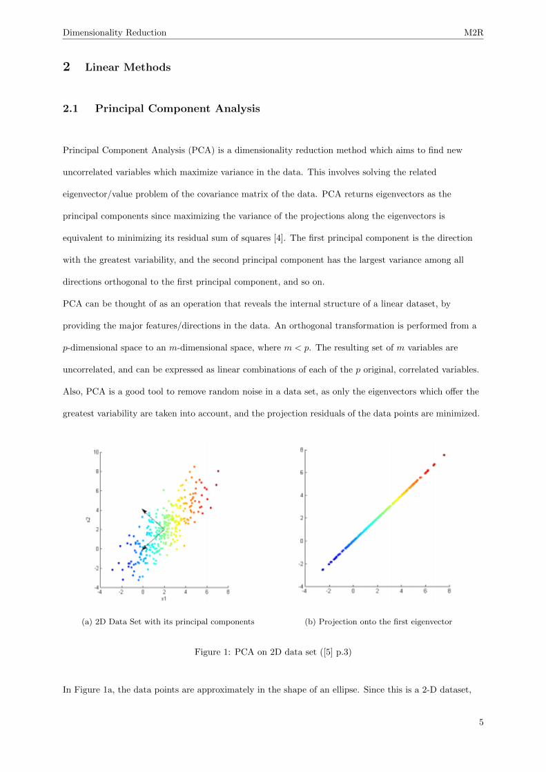
(a) 2D Data Set with its principal components (b) Projection onto the first eigenvector

Figure 1: PCA on 2D data set ([5] p.3)

In Figure 1a, the data points are approximately in the shape of an ellipse. Since this is a 2-D dataset,

5


there will be 2 principal components. It is clear from the images above that the major axis of the ellipse

is the eigenvector that offers the greatest variability, and thus, it is the first principal component. The

second principal component, being orthogonal to the the first, will be the minor axis. Taking only the

first principal component and projecting the data points onto it, we can see that a straight line is

obtained (as seen in Figure 1b). Thus, the dimensionality of the dataset is now 1, and it is expressed in

terms of this eigenvector.

2.1.1 Procedure

1. Suppose we have a p dimensional set of data, and n observations. We therefore intend to find the

first m principal components, where m < p. Place the data in an n× p matrix, called X. Then, let

y ∈ Rp be the vector that contains the means of the columns of X, i.e.

yj =1

n

n∑i=1

Xij

2. Subtract the mean from each column, to obtain a matrix A

A = X − hyT

where h is a n x 1 vector of ones. This is done to center the data around the origin. The matrix A

should take the form

A =

x11 − y1 . . . x1p − yp

.... . .

...

xn1 − y1 . . . xnp − yp

3. Calculate the covariance matrix of the data, Σ. This is done by taking the inner product of A with

itself. It is then divided by n− 1 to account for the bias of the variance in a random sample.

Σ =1

n− 1ATA

4. Find the eigenvalues and eigenvectors of Σ. Form the matrix P of eigenvectors and its associated

diagonal matrix D such that

Σ = PDPT

Since Σ is a symmetric, positive definite p× p matrix, it has p distinct eigenvalues, and p linearly

independent eigenvectors, meaning that such matrices P and D exist.

6


Rearrange the entries of D and P so that the eigenvalues in D are in decreasing order. It is also

important the eigenvectors in P should be of unit length.

5. Pick the first m columns of P as the principal components of the data. These should be the

eigenvectors which have the largest eigenvalues of Σ. To avoid too much loss of information, m is

appropriately chosen so that ∑mi=1 λi∑pj=1 λj

≥ π

where λ1, λ2, . . . ,λp are the eigenvalues of Σ in order of decreasing size. π is the minimum

proportion of total variance that we would like to account for, and is a subjective threshold to

decide on the number of principal components, m, to be retained. Normally, greater weight is

placed on the components with the greatest variability, but there are circumstances in which the

last few may be of interest, such as in outlier detection or some applications of image analysis [6].

6. The final step of the PCA is to perform the change of coordinates, such that the orthogonal

principal components chosen form the axes of the new dataset. We form the matrix X as follows:

X = PTA

where the columns of P are the first m eigenvectors of P . This gives us the data in terms of the

principal components that we have chosen. [7]

2.1.2 PCA for Image Processing

Image processing is one of the most important uses of PCA at the moment. Suppose we have 50 images,

each of dimension 200,000. To perform the PCA, each pixel in each image is converted into a number

from 0 to 255, representing the intensity on the greyscale. Then, similar to the algorithm explained

above, images of large dimensions are broken down, and a set of eigenvectors is obtained. When

converted back to images, these vectors are known as eigenfaces or eigenimages . These are just the

features on the images that give the greatest variability in the set of images, for example, the eyes or the

shape of the faces. Once this is done, each individual image is expressed as a weighted sum of these

eigenfaces and reconstructed. [8] This image processing feature is then used for facial recognition and

verification software, commonly used in surveillance as well as biometric security. [9]

7


2.2 Multi-Dimensional Scaling

‘Multidimensional scaling (MDS) is a method that represents measurements of similarity (or

dissimilarity) among pairs of objects as distances between points of a low-dimensional multidimensional

space.’ ([10], p.3)

2.2.1 Motivating Example

Figure 2 represents the flying distances between 10 American Cities. We attempt to find 2-Dimensional

coordinates of the cities. (Figure 3)

Figure 2: Flying Mileages between 10 American cities [11]

Figure 3: Classical MDS of flying mileages between 10 American cities [11]

2.2.2 Classical Multi-Dimensional Scaling

Goal: Suppose we know that we have n p-dimensional data points. Given only the distance matrix

between the data points, we determine these data points.

That is, given the distance matrix d11 . . . d1n

.... . .

...

dn1 . . . dnn

8


where dij is the Euclidean distance between xi and xj . We then attempt to find the matrix X:

X =

x1

...

xn

where each xi is a p-dimensional data point.

2.2.3 Procedure

Write T = XXT .

d2ij = (xi − xj)T (xi − xj)

= xTi xi + xTj xj − 2xTi xj

= Tii + Tjj − 2Tij

This can be rearranged to obtain

Tij = −1

2[d2ij − Tii − Tjj ]

= −1

2[d2ij − di. − d.j + d2..]

where

d2i. =1

n

n∑j=1

d2ij , d2.j =1

n

n∑i=1

d2ij , d2.. =1

n2

n∑j=1

n∑i=1

d2ij

This is equivalent to writing

T = JAJ, where Aij = d2ij , J = I − 1

nhhT

and h is an n× 1 vector of ones.

T = XXT =⇒ T is symmetric and positive definite

=⇒ T is diagonalizable

=⇒ T = UΛUT

Also, T has non-negative eigenvalues, and rank T = rank(XXT ) = rank X = p. This means that T has

p positive eigenvalues and n− p eigenvalues identically equal to zero.

9


(Here we are assuming that p < n.)

T = UΛUT

= (UΛ12 )Λ

12UT

= (UΛ12 )(UΛ

12 )T

Then X = UΛ12 . Since there are n− p eigenvalues equal to 0, X = U ′Λ′

12 , where

U ′ =

| |

v1 . . . vp

| |

, Λ′ =

λ1

. . .

λp

where v1, . . . , vp are the eigenvectors of T corresponding to the non-zero eigenvalues λ1, . . . , λp. [2] [12]

2.2.4 Application to Dimensionality Reduction

Given the matrix X, containing n data points in p dimensions,

X =

x1

x2

...

xn

n x p

where xi are the n data points. We compute the n× n distance matrix:

D =

d11 . . . d1n

.... . .

...

dn1 . . . dnn

with dij is the distance between the ith and jth data point.

From the above procedure: X = U ′Λ′12 . We can order the eigenvalues of Λ′ in decreasing order to

obtain Λ and rearrange the eigenvectors in U ′ accordingly to obtain U . The matrix X = U Λ12 still correctly

represents the data.

The reduction of data in X to m dimensions where m < p is obtained by picking out the first m

columns of U and Λ12 .

The classical MDS as given above minimises the following loss function:

∑1≤i≤j≤n

(δij − dij)2

10


where δij represents the distance betwwen points i and j in the lower dimensional space, and dij is as above.

Given a data set, reducing the dimensionality using Classical Multidimensional Scaling actually gives

the same result as applying Principal Component Analysis. [1] [2]

2.2.5 Extensions to the Classical MDS

• The algorithm can be adapted to minimise different loss functions. For example, the weighted loss

function as follows can be minimized.

∑1≤i≤j≤n

aij(δij − dij)2

This class of multidimensional scaling is known as metric MDS.

• Non-Metric MDS: instead of preserving the distances between the points, the rank of the similarity

between the data points is preserved i.e. if point x1 is closer to x2 than to x3 in the original

dimensions then this property is preserved after dimensionality reduction.

This is especially useful when the input data points are qualitative. A dissimilarity matrix is built

and Non-Metric MDS applied to this matrix. [2] [12]

2.3 Limitations of Linear Techniques

The limitations of the linear dimensionality reduction methods (including the PCA and MDS) stem from

the fact that it is a linear transformation. This is major problem as many real-world data sets are non-

linear, and the above algorithms fail to capture this. As a knock-on effect, small perturbations in non-linear

data can have big influences in the principal components and the eigen-representation. [8]

With the PCA, one assumption the algorithm makes is that the directions with the largest variance

are assumed to be the most important. While this is usually the case, the following is an example where

it is not. Suppose we have sets of data stacked on top of each other (like pancakes), and we want to

cluster these sets together. The PCA is going to say that the length and breadth of the ‘pancakes’ are

the principal components. However, to separate these clusters of data we would be more interested in the

height axis of the data, and in this case, it is the axis of smallest variance. [13]

11


3 Non-Linear Methods

3.1 Locally Linear Embedding

Locally Linear Embedding (LLE) is a non-linear dimensionality reduction technique which aims to preserve

neighbourhood relations. The algorithm characterizes the local geometry of the dataset by finding linear

coefficients that reconstruct each data point from its neighbouring points. With linear methods such as

the PCA or MDS discussed earlier, faraway data points on non-linear manifolds are mapped to nearby

points in the plane, and thus the underlying structure of the manifold cannot be properly identified by

these algorithms.

Suppose there are n data points, x1, . . . xn each of dimensionality p. We want to map these data points

onto a m-dimensional space, where m < p. [14][15]

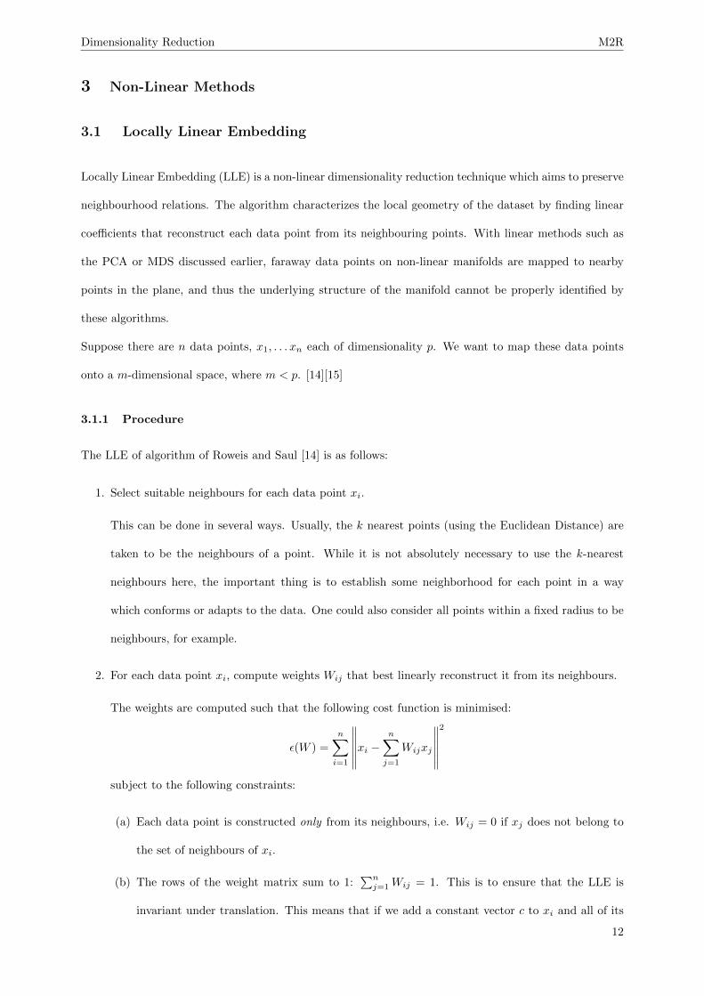
3.1.1 Procedure

The LLE of algorithm of Roweis and Saul [14] is as follows:

1. Select suitable neighbours for each data point xi.

This can be done in several ways. Usually, the k nearest points (using the Euclidean Distance) are

taken to be the neighbours of a point. While it is not absolutely necessary to use the k-nearest

neighbours here, the important thing is to establish some neighborhood for each point in a way

which conforms or adapts to the data. One could also consider all points within a fixed radius to be

neighbours, for example.

2. For each data point xi, compute weights Wij that best linearly reconstruct it from its neighbours.

The weights are computed such that the following cost function is minimised:

ε(W ) =

n∑i=1

∥∥∥∥∥∥xi −n∑

j=1

Wijxj

∥∥∥∥∥∥2

subject to the following constraints:

(a) Each data point is constructed only from its neighbours, i.e. Wij = 0 if xj does not belong to

the set of neighbours of xi.

(b) The rows of the weight matrix sum to 1:∑n

j=1Wij = 1. This is to ensure that the LLE is

invariant under translation. This means that if we add a constant vector c to xi and all of its

12


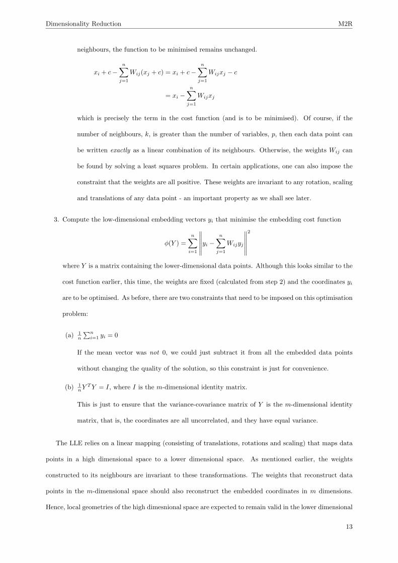
neighbours, the function to be minimised remains unchanged.

xi + c−n∑

j=1

Wij(xj + c) = xi + c−n∑

j=1

Wijxj − c

= xi −n∑

j=1

Wijxj

which is precisely the term in the cost function (and is to be minimised). Of course, if the

number of neighbours, k, is greater than the number of variables, p, then each data point can

be written exactly as a linear combination of its neighbours. Otherwise, the weights Wij can

be found by solving a least squares problem. In certain applications, one can also impose the

constraint that the weights are all positive. These weights are invariant to any rotation, scaling

and translations of any data point - an important property as we shall see later.

3. Compute the low-dimensional embedding vectors yi that minimise the embedding cost function

φ(Y ) =

n∑i=1

∥∥∥∥∥∥yi −n∑

j=1

Wijyj

∥∥∥∥∥∥2

where Y is a matrix containing the lower-dimensional data points. Although this looks similar to the

cost function earlier, this time, the weights are fixed (calculated from step 2) and the coordinates yi

are to be optimised. As before, there are two constraints that need to be imposed on this optimisation

problem:

(a) 1n

∑ni=1 yi = 0

If the mean vector was not 0, we could just subtract it from all the embedded data points

without changing the quality of the solution, so this constraint is just for convenience.

(b) 1nY

TY = I, where I is the m-dimensional identity matrix.

This is just to ensure that the variance-covariance matrix of Y is the m-dimensional identity

matrix, that is, the coordinates are all uncorrelated, and they have equal variance.

The LLE relies on a linear mapping (consisting of translations, rotations and scaling) that maps data

points in a high dimensional space to a lower dimensional space. As mentioned earlier, the weights

constructed to its neighbours are invariant to these transformations. The weights that reconstruct data

points in the m-dimensional space should also reconstruct the embedded coordinates in m dimensions.

Hence, local geometries of the high dimesnional space are expected to remain valid in the lower dimensional

13


Figure 4: The LLE algorithm [14]

space. The implementation of the LLE algorithm is also rather straightforward, as it only has one free

parameter, which is k, the number of neighbours we chose for each data point.

3.2 Diffusion Maps

3.2.1 Theory

We define the connectivity of two data points, xi, xj ∈ S, where S = {xl}nl=1 is the data set, to be the

probability of jumping from xi to xj in one step of a random walk. We can express this connectivity in

terms of a ‘kernel’, which defines a measure of similarity within a certain neighbourhood and the function

is almost zero outside of the neighbourhood. The kernel satisfies the following properties:

1. k(xi, xj) = k(xj , xi)

2. k(xi, xj) ≥ 0

These properties allow us to follow the process of diffusion maps, as we shall see later on.

The most commonly used kernel in the literature on this topic [16][17] is the Gaussian kernel, which is

14


defined as

k(xi, xj) = exp

(−‖xi − xj‖

2

α

)(1)

We choose ε such that 0 < ε � 1 and the neighbourhood of xi is defined as the set of xj such that

k(xi, xj) > ε. We can change ε and α to vary the properties of the neighbourhood.

We define d(xi):

d(xi) =∑y∈S

k(xi, y) (2)

Then the probability of jumping from xi to xj in one step of a random walk, or the connectivity of xi and

xj can be expressed by:

p(xi, xj) =1

d(xi)k(xi, xj) (3)

d(xi) is the normalizing constant and we see that the sum, over all the points y in the data set S, of

probabilities of jumping from xi to y is 1.

∑y∈S

p(xi, y) =∑y∈S

1

d(xi)k(xi, y)

=1

d(xi)

∑y∈S

k(xi, y)

= 1

We can now define a matrix P , with entries Pij = p(xi, xj) where xi, xj ∈ S, to be the diffusion matrix.

The i, jth entry is the connectivity between data points xi and xj . In the parallel study of a random walk,

we would say that each entry represents the probability of jumping from point i to point j in one step. We

can take this matrix to the power t and note that we now have entries equal to the probability of going

from point i to point j in a random walk of t steps. For example, with 3 points and two steps,p11 p12 p13

p21 p22 p23

p31 p32 p33

2

=

p211 + p12p21 + p13p31 p11p12 + p12p22 + p13p32 p11p13 + p12p23 + p13p33

p21p11 + p22p21 + p23p31 p21p12 + p222 + p23p32 p21p13 + p22p23 + p23p33

p31p11 + p32p21 + p33p31 p31p12 + p32p22 + p33p32 p31p13 + p32p23 + p233

In order to find the underlying structure of the dataset, we take P to a number of powers that has to be

determined. If we take it to too high a power then we will have so many steps in our random walk that

all points will be well connected. If we take too small a power, we may be limiting the number of steps

in our random walk to the extent that we don’t get a proper appreciation of the underlying geometry of

15


the data. Random walks along the data with lots of small steps will have a much higher probability than

those with any big steps. These small-step paths will follow the underlying structure of the data.

We now define the diffusion distance to be

Dt(xi, xj)2 =

∑y∈S‖pt(xi, y)− pt(xj , y)‖2 (4)

=

n∑m=1

‖(P t)im − (P t)mj‖2 (5)

where S = {x1, . . . , xn}. We define pt(xi, xj) = (P t)ij . We have not yet defined which metric, ‖ · ‖, we

are using. It should be noted that this distance doesn’t suffer from the effects of noise, as it sums over

all paths between the two points. pt(·, ·), in the analogy to a random walk, represents the probability of

going from one point to another in t steps.

As paths that aren’t on the underlying structure of the dataset will have small probabilities, the most

influencial paths on the diffusion distance will be those on the underlying structure. If points x and y are

well connected, the probabilities for paths between x and w, and y and w, where w is a third point, will

be similar.

It may be apparent that calculating diffusion distances is a time consuming process and therefore it is

best to map the data points into a Euclidean space with distance between the mapped points the same as

the diffusion distance between the original points. We call this new Euclidean space the ‘diffusion space.’

The map between the space containing the data points and the diffusion space is the diffusion map. The

diffusion map will preserve the geometry of the data points which we assume to be of lower dimension

than the space containing the data points. In this case, preservation of geometry is expressed by diffusion

distances being equal to new Euclidean distances, as above. A good approximation for that Euclidean

distance can be obtained in a diffusion space of fewer dimensions that the original data space, as we shall

see.

Define

Yi :=

pt(xi, x1)

...

pt(xi, xn)

= [(P t)i]T (ith row of P t, transposed) (6)

16


Now, the distance between Yi and Yj , in any metric, squared, is

‖Yi − Yj‖2 =∑y∈S‖pt(xi, y)− pt(xj , y)‖2

= Dt(xi, xj)2 in that metric (7)

We now have the distance between Yis to be the same as the diffusion distance, but we have no dimension

reduction. We must find a way of ignoring the least important dimensions of the diffusion space. We use

the following:

Lemma

Suppose K is a symmetric, n× n kernel matrix such that Kij = k(xi, xj). Then, we can use the diagonal

matrix D = diag(d(x1), . . . , d(xn)) to normalise K and produce a diffusion matrix

P = D−1K. (8)

Then, the matrix P ′, defined as

P ′ = D1/2PD−1/2, (9)

1. is symmetric,

2. has the same eigenvalues as P

3. has eigenvectors xk such that when multiplied by D−1/2 and D1/2 give the left and right eigenvectors

of P , respectively.

Proof

P ′ = D1/2PD−1/2

= D1/2D−1KD−1/2

= D−1/2KD−1/2

K is symmetric, so P ′ will also be symmetric. P ′ being symmetric implies that we can find Q and V such

that

P ′ = QV QT

17


where V is diagonal and contains the eigenvalues of P ′, and Q’s columns are orthonormal eigenvectors of

P ′. Q is orthogonal so Q−1 = QT . Now,

P = D−1/2P ′D1/2

= D−1/2QV QTD1/2

= D−1/2QV Q−1D1/2

= (D−1/2Q)V (D−1/2Q)−1

= ZV Z−1 (10)

for Z = D−1/2Q. We see that the eigenvalues of P and P ′ are the same. Also, the right eigenvectors of P

are the columns of Z and the left eigenvectors of P are the rows of Z−1 = QTD1/2. This implies that the

right eigenvectors of P are

vl = D−1/2xl (11)

where xl is an eigenvector of P ′.

Similarly for the left eigenvectors of P ,

ul = D1/2xl. � [17] (12)

Then, by (10), we have

P =

n∑k=1

λkvkuTk (13)

Also,

P t = (ZV Z−1)t

= ZV tZ−1

=

n∑k=1

λtkvkuTk (14)

We notice that the ith row of P t can be written as a sum of the left eigenvectors as follows

(P t)i =

n∑k=1

λtkvk(i)uTk (15)

where vk(i) is the ith entry of vk.

The left eigenvectors are a basis for the rows of P t so we can represent the rows of P t as vectors in the

18


co-ordinate system with the left eigenvectors as the basis. Note that we can write the ith row of P t, in

this new co-ordinate system, as

Li =

λt1v1(i)

...

λtnvn(i)

(16)

The issue is that this will almost definitely not be an orthonormal basis. However, the basis of eigenvectors

of P ′ was orthonormal and we use this fact to get an inner product for which the left eigenvectors are an

orthonormal basis.

1 = xTk xk for all k ∈ {1, . . . , n}

= (D−1/2uk)T (D−1/2uk) by (12)

= uTkD−1uk

0 = xTi xj for i 6= j with i, j ∈ {1, . . . , n}

= (D−1/2ui)T (D−1/2uj) by (12)

= uTi D−1uj

We see that the left eigenvectors of P are orthonormal under the inner product using the matrix D−1.

D−1 is a diagonal matrix with positive entries so is clearly a symmetric, positive definite matrix and the

inner product is well defined.

19


We can calculate the Euclidean distance squared between Li and Lj for i, j ∈ {1, . . . , n}.

‖Li − Lj‖2E =

n∑k=1

λ2tk (vk(i)− vk(j))2

=

n∑l=1

n∑k=1

xTl xkλ

tl(vl(i)− vl(j))λ

tk(vk(i)− vk(j)) as the vectors {xq}nq=1 are orthonormal

=

n∑l=1

xTl λ

tl(vl(i)− vl(j))

n∑k=1

xkλtk(vk(i)− vk(j))

=

(n∑

l=1

xTl λ

tl(vl(i)− vl(j))D

1/2

)D−1

(D1/2

n∑k=1

xkλtk(vk(i)− vk(j))

)

=

(n∑

l=1

xTl λ

tl(vl(i)− vl(j))D

1/2

)D−1

(n∑

k=1

xTkλ

tk(vk(i)− vk(j))D1/2

)T

=

∥∥∥∥∥n∑

k=1

xTkλ

tk(vk(i)− vk(j))D1/2

∥∥∥∥∥2

[D−1]

=

∥∥∥∥∥n∑

k=1

xTkD

1/2λtk(vk(i)− vk(j))

∥∥∥∥∥2

[D−1]

=

∥∥∥∥∥n∑

k=1

λtkuTk (vk(i)− vk(j))

∥∥∥∥∥2

[D−1]

by (12)

=

∥∥∥∥∥n∑

k=1

λtkuTk vk(i)−

n∑k=1

λkuTk vk(j)

∥∥∥∥∥2

[D−1]

=∥∥(P t)i − (P t)j

∥∥2[D−1]

by (15)

= ‖Yi − Yj‖2[D−1] by (6)

= Dt(xi, xj)2[D−1] by (7)

This shows us that the diffusion distance in the space containing the data points is the same as the

Euclidean distance in the diffusion space. We notice that our calculations of Euclidean distance in the

diffusion space are most affected by the dominant eigenvalues. We can reduce to m dimensions by taking

only the co-ordinates of Li in the dimensions corresponding to the dominant eigenvalues.

3.2.2 Procedure

Given a n-dimensional data set, {xi}ni=1, the basic algorithm for a diffusion map dimensionality reduction

is as follows:

1. Define a kernel k(x, y) with properties as defined above. Create a kernel matrix, K, with Kij =

k(xi, xj).

2. Find the sum of each of the rows of K and for the ith row, call this d(xi). Construct the diagonal

20


matrix D = diag(d(x1), . . . , d(xn)). Use this to find the diffusion matrix P = D−1K.

3. Decide how many dimensions you want the diffusion space to be (say m) and find the m most

dominant eigenvalues of the diffusion matrix and their corresponding eigenvectors.

4. Map into the lower dimensional diffusion space at time t, by using (16) but only including the entries

corresponding to the m dominant eigenvalues. These vectors are your new lower dimensional data

in the diffusion space, {yi}ni=1

21


4 Comparison of PCA and Diffusion Maps

In this section we will compare the performance of PCA and Diffusion Maps on two different data sets,

both of which contain 1000 data points in 3 dimensions. The data sets are both generated according to a

one-dimensional underlying parameter and perturbed by some noise. To assess the two methods, we will

perform dimensionality reduction on the data sets, and then see if the first non-trivial co-ordinate of the

reduced data is in one-to-one correspondence with the underlying parameter.

4.1 Linear Dataset

The first data set we look at is generated by the following formula.3

7

−1

T + ε

where T is the underlying parameter of the data set and is sampled from a Uniform(0,10) distribution and

ε is sampled from a MVN(0,I3) distribution and acts as a small noise perturbation.

The data is plotted in Figure 5.

Figure 5: Plot of the Linear Data set

22


(a) PCA (b) Diffusion Map

Figure 6: Plot of T vs reduced co-ordinates


Figure 7: Plot of the Linear data set coloured using the PCA and Diffusion Map co-ordinate

From Figure 6, we see that for both PCA and Diffusion Maps, the parameter T is monotonic with the

first non-trivial co-ordinates of the reduced data.

Figure 7 shows a plot of the original data with points coloured from red to blue according to the deciles

of the first non-trivial co-ordinates of the reduced data.

4.2 Non-Linear Dataset

The second data set was generated by the following formula:

A

cos(A)

sin(A)

cos(3A)

+ε

30

where A is the underlying parameter sampled from a Uniform(0,2π) distribution and ε is sampled from a

MVN(0,I3) distribution and again acts as a noise perturbation.

23


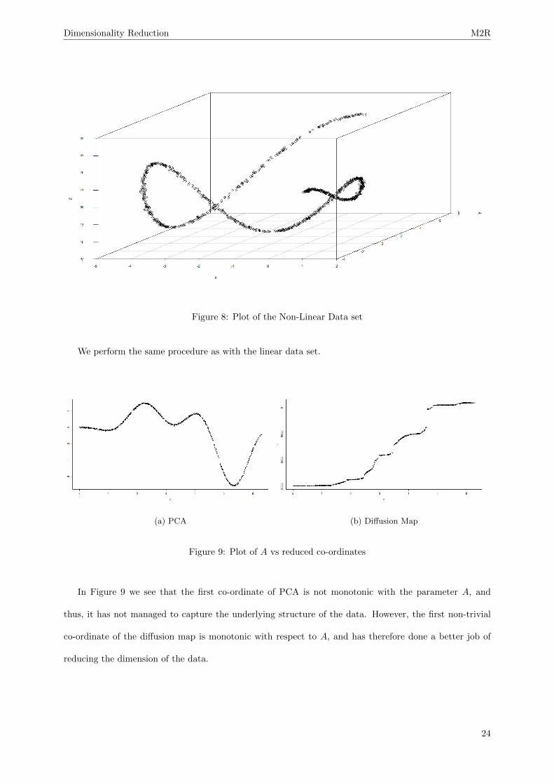
Figure 8: Plot of the Non-Linear Data set

We perform the same procedure as with the linear data set.


Figure 9: Plot of A vs reduced co-ordinates

In Figure 9 we see that the first co-ordinate of PCA is not monotonic with the parameter A, and

thus, it has not managed to capture the underlying structure of the data. However, the first non-trivial

co-ordinate of the diffusion map is monotonic with respect to A, and has therefore done a better job of

reducing the dimension of the data.

24



Figure 10: Plot of the Non-Linear data set coloured using the PCA and Diffusion Map co-ordinate

In Figure 10 we can see clearly that when coloured by the Diffusion Map co-ordinate, our plot changes

from red to blue monotonically as we travel along the curve. However, with the PCA co-ordinate, the

colour changes from purple to blue to red to purple again, showing that PCA has not found the underlying

structure of the data. [18] [22][24][25]

25


5 Clustering and dimensionality reduction applications

5.1 Clustering

5.1.1 Theory

‘Data clustering (or just clustering), also called cluster analysis, segmentation analysis, taxonomy analysis,

or unsupervised classification, is a method of creating groups of objects, or clusters, in such a way that

objects in one cluster are very similar and objects in different clusters are quite distinct.’ ([19],p.1)

Several methods relying on different notions of similarity are used to cluster the data. Some common

clustering methods are:

• Hierarchical Clustering

A hierarchy of clusters is obtained. There are two ways of going about hierarchical clustering: an

agglomerative approach and a divisive approach.

The agglomerative approach consists of starting with n individual clusters and progressively merging

the two most similar clusters at each stage until a single cluster is obtained. The divisive approach

involves starting with a single cluster and progressively splitting the clusters until n clusters each

containing a single data point is obtained.

An example of a hierarchical cluster of the data points p, q, r, s, t is

26


Figure 11: Example of a hierarchical cluster of the data points p, q, r, s, t [20]

• Distribution Clustering

Clusters are created by grouping data which are more likely to be drawn from the same distribution.

Different clusters may be described by a distribution with different parameters or they may be

described by altogether different distributions.

• Sums of Squares Clustering

Clusters are created such that the intra-cluster sum of squares is minimized. k-means clustering is

an example of Sums of Squares Clustering.

k- means clustering minimizesk∑

j=1

∑xi∈Cj

‖xi − cj‖2

where cj is the cluster centre of the cluster Cj . [2]

For this project we will use the k-means Clustering method. It is one of the most popular clustering

methods as it is fast and it is easily implemented. k-means clustering can however be sensitive to the

chosen starting points of the algorithm. It also requires the number of clusters to be defined by the user.

5.1.2 Procedure

The k-means clustering algorithm is as follows:

1. Randomly choose k points as cluster centres.

27


2. Each data point is placed in the cluster whose cluster centre it is closest to.

3. Calculate new cluster centres by setting them to the mean of the points in their corresponding cluster.

4. Each data point is again placed in the cluster whose cluster centre it is closest to.

5. Repeat Steps 2 and 3 until none of the data points change cluster, or until a specified maximum

number of iterations is reached. [12]

(a) Given these data points (b) Connect all data points to the nearest cluster centre

(c) Find the new cluster centres (d) Repeat (b) and (c) until no data points change clusters

Figure 12: Visualiztion of the k-means clustering algorithm [21]

5.2 Use of Diffusion Maps in Clustering

In this section we will give an example where Diffusion Maps can help cluster non-linear data with the

k-means algorithm. We will use a ‘Chainlink’ toy clustering data set [26], which has 1000 data points in 3

dimensions that form the shape of two interlocked rings (shown in figure 13). We would like our clustering

technique to identify each ring as a separate cluster. We will try applying the k-means algorithm to the

28


Figure 13: Plot of the Chainlink data set [26]

data set in its original co-ordinates. We will also try computing the diffusion co-ordinates of the data

set and then applying the k-means algorithm to the data in the diffusion co-ordinates and compare the

results. Note that in both cases we will use k=2 as the number of clusters for k-means.

29


(a) K-Means applied directly (b) K-Means applied to Diffusion Map co-ordinates

Figure 14: Plot of Clustered data set

We can see in figure 14(a) that K-means applied directly to the data set fails to identify the two rings

as clusters, this is because it uses Euclidean distances. Transforming the data into diffusion co-ordinates

allows us to identify each ring as as separate cluster.

This occurs because the diffusion distance between two points is small if they are connected by lots of

points which are close together, and so any two points within the same ring will have small diffusion

distance between them. On the contrary, points in separate rings will have large diffusion distance, as

there is a low probability of ’jumping’ from one ring to the other in the diffusion process. [22][24]

30


5.3 Application to Image Processing

In this section we will be investigating the data set shown in figure 15

(a) Our data set

(b) 2 original images [27]

Figure 15

This data set consists of 2 different images, each rotated 40 times. The images are each 160x160 pixels,

each with 3 RGB values, and so our data set has size n = 80, with p = 76800 (160 × 160 × 3) variables.

We would like to have an algorithm that can separate the data into two clusters, each containing the

rotations of one of the original images.

We will first try applying k-means directly to the data set, and then try applying k-means to the data set

reduced to diffusion co-ordinates (using k=2 in both cases). We ran both algorithms 1000 times; the total

run time and number of times the algorithms successfully cluster the data set into clusters of the original

images are shown in Figure 16.

It is clear that in this case applying k-means to the data in diffusion co-ordinates is both faster to run,

and more successful.

31


Time (s) # Successes

Direct k-means 918.97 114

Diffusion k-means 18.97 988

Figure 16

Figure 17: Plot of the data set with respect to the first and second Diffusion co-ordinates

In figure 17 we have reduced the dimension of the data to the first 2 diffusion co-ordinates so that we

can plot it and therefore more easily visualise it. The two images are clearly separated into two clusters

as expected from our clustering results above.

Now we would like to investigate whether the Diffusion Map has managed to maintain the underlying

structure of the data; since the data within each cluster are generated by a one dimensional parameter

(degree of rotation), we can imagine that the data points approximately lay on some curve in Rp space,

with degree of rotation monotonically increasing as we travel along the curve. We would like the same to

be true in our reduced data set.

32


Figure 18: Close up of each cluster

We can see clearly in figure 18 that each cluster forms a curve, and as we travel along each curve, the

degree of rotation of the image changes monotonically. Therefore even though we have drastically reduced

the dimension of the data, from 76800 to 2, we have preserved the underlying structure. [22][23]

33


6 Application to financial data

In this section, we will show some of the things that dimensionality reduction allows you to do in the study

of large data sets. We take the data for the S&P 500 from 1st November 2014 to 9th November 2015 [28].

We treat each of the 494 companies as a 259 dimensional data point. 259 is the number of days on which

business was done between the above dates. We will use Diffusion Maps to reduce to two dimensions and

then use k-means clustering to get an impression of which companies’ stock prices tend to follow similar

paths.

Before analysing the data, we normalised all of the data points. We did this to best evaluate companies

whose stock prices follow similar paths relative to their means as well as relative to their stock price. This

is necessary in order to compare companies with vastly different stock prices. For example, Netflix’s stock

price varies from about 100 to 700 over the time period, averaging about 350, whilst Xerox’s stock price

varies from 9.5 to 15, averaging 12. First, we found the mean, Xi, of every company’s stock prices over

the year and standard deviation, si. For a company’s data, Xi, we performed the following:

Xi →1

si

Xi −

Xi

...

Xi

The following is a scatterplot of the first two diffusion coordinates with the ten large black spots represent-

ing the centroids of the clusters. It should be noted that the choice of k = 10 for the k-means algorithm

is, in this example, somewhat arbitrary. Anywhere between 6 and 15 clusters is reasonable and this is

probably due to the sparsity of the data with the first diffusion co-ordinate between −2 and 2, as can be

seen in the figure.

34


Figure 19: Scatterplot of first two diffusion co-ordinates and cluster centroids

Figure 20 shows the points in their clusters where each cluster is a different colour:

Figure 20: Scatterplot of colour clustered points

We had originally surmised that companies in a similar industry should follow similar paths. We found

this to be false for all industries other than energy. Figure 21 a plot of the diffusion coordinates with

energy companies highlighted.

35


Figure 21: Scatterplot with energy companies highlighted

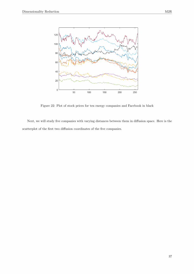
We see that the large majority of the energy companies are in the left most cluster. We now plot the

stock prices of ten of the energy companies in Figure 22 and note they follow similar paths. We have

included the black line which is Facebook’s stock prices for contrast.

36


Figure 22: Plot of stock prices for ten energy companies and Facebook in black

Next, we will study five companies with varying distances between them in diffusion space. Here is the

scatterplot of the first two diffusion coordinates of the five companies.

37


Figure 23: Plot of diffusion coordinates for 5 companies

We compare the plots of the companies’ normalised stock prices as opposed to the full stock prices

compared in the example with energy companies. This is because Google’s stock price dwarfs those of the

others to the extent that they all look like straight lines.

38


Figure 24: Comparing plots for the 5 companies

It is quite clear that Google and Facebook follow the most similar paths. This is exactly what we

expected as they cluster together and have diffusion coordinates that are very close to each other. None

of the other companies follow paths that are particularly similar to each other.

One of the most important things that we saw in this data set was the increase in computational efficiency

due to diffusion maps. The MATLAB function for direct k-means on the full data set took, on average,

about 13 seconds, whilst diffusion maps and k-means on the diffusion coordinates took just over a second.

It is interesting to note that for this data set, we get similar results from PCA, with very similar clustering,

as well as computational efficiency increases. [29]

39


7 Conclusion

Dimensionality reduction is an important tool in data analysis as it allows us to more easily visualise data,

reduce computation time, and apply statistical techniques that may fail in high dimensions.

We have investigated linear and non-linear dimensionality reduction techniques, and have outlined limita-

tions with linear methods.

With particular focus on Diffusion Maps, we demonstrated applications in image processing; and in cluster

analysis which we applied to real financial data.

40


References

[1] Lee J.A., Verleysen M. Nonlinear Dimensionality Reduction. Springer Series Information Science and

Statistics. New York: Springer 2007.

[2] Webb A.R., Copsey K.D. Statistical Pattern Recognition 3rd Edition. UK: John Wiley & Sons, Ltd.

2011.

[3] Verleysen M, Francois D. The Curse of Dimensionality in Data Mining and Time Series Prediction.

In: Cabestany J., Prieto A., Sandoval F. (eds) Computational Intelligence and Bioinspired Systems.

2005.Volume 3512 of the series Lecture Notes in Computer Science p 758-770

[4] Shalizi C. Principal Components Analysis. Carnegie Mellon University; 2009 pp36 - 350. Available

from http://www.stat.cmu.edu/ cshalizi/uADA/12/lectures/ch18.pdf [Accessed 5th June 2016]

[5] Socher, R. Manifold Learning and Dimensionality Reduction Available from:

http://www.socher.org/uploads/Main/DiffusionMapsSeminarReport RichardSocher.pdf [Accessed

2nd June 2016]

[6] Joliffe I.T., Cadima J. Philosophical transactions. Series A, Mathematical, physical, and engineering

sciences Principal Component Analysis: A Review and Recent Developments. 2016, Vol.374(2065),

pp.20150202 Avaiable from DOI: 10.1098/rsta.2015.0202.

[7] Smith L.I. A Tutorial on PCA. Available from:

http://www.cs.otago.ac.nz/cosc453/student tutorials/principal components.pdf [Accessed 26th May

2016]

[8] Hlavac V. Principal Component Analysis Application to images. Czech Technical University in Prague.

http://cmp.felk.cvut.cz/ hlavac/TeachPresEn/11ImageProc/15PCA.pdf [Accessed 28th May 2016]

[9] Mahvish Nasir. What is PCA (Explained from face recognition point of view). 2013; Available from

https://www.youtube.com/watch?v=g5 tonFnfaQ [Accessed 1st June 2016]

[10] Ingwer B., Groenen P.J.F. Modern Multidimensional Scaling Theory and Applications. 2nd

Edition. Springer Series in Statistics. Springer-Verlag New York Inc 2007. Avaliable from

http://link.springer.com/book/10.1007/0-387-28981-X/page/1 [Accessed 3rd June 2016]

41


[11] Young F.W. MULTIDIMENSIONAL SCALING Available from

http://forrest.psych.unc.edu/teaching/p208a/mds/mds.html [Accessed 3rd June 2016]

[12] Vathy-Fogarassy A., Janos A.Graph-Based Clustering and Data Visualization Algorithms.

SpringerBriefs in Computer Science. London: Springer- Verlag 2013. Available from

http://link.springer.com/book/10.1007/978-1-4471-5158-6/page/1/ [Accessed 7th June 2016]

[13] What are some of the limitations of principal component analysis? Available from:

https://www.quora.com/What-are-some-of-the-limitations-of-principal-component-analysis [Ac-

cessed 3rd June 2016]

[14] Roweis S.T., Saul L.K. Nonlinear Dimensionality Reduction by Locally Linear Embedding. Science

Magazine. 2000; 290(5500), :2323-2326

[15] Shalizi C. Non-Linear Dimensionality Reduction I: Local Linear Embedding. Carnegie Mellon Uni-

versity; 2009 pp36 - 350. Available from http://www.stat.cmu.edu/ cshalizi/350/lectures/14/lecture-

14.pdf [Accessed 3rd June 2016]

[16] De la Porte J, Herbst B.M., Hereman W., Van Der Walt S.J. An introduction to diffusion maps. In:

Proceedings of the 19th Symposium of the Pattern Recognition Association of South Africa (PRASA

2008), Cape Town, South Africa 2008 Nov 26 (pp. 15-25).

[17] Coifman RR, Lafon S. Diffusion maps. Applied and computational harmonic analysis. 2006;21(1):5-30.

[18] Bubacarr B. Diffusion Maps: Analysis and Applications. MSc thesis. University of Oxford;2008

[19] Gan G., Ma C. and Wu J. Data Clustering: Theory, Algorithms, and Applications Philadelphia, PA

19104 ASA-SIAM Series on Statistics and Applied Probability, SIAM, , ASA, Alexandria, VA, 2007.

[20] Front Line Solvers. HIERARCHICAL CLUSTERING. Available from

http://www.solver.com/xlminer/help/hierarchical-clustering-intro [Accessed 9th June 2016]

[21] Shabalin, Andrey A. [Animated gifs.] Available from http://shabal.in/visuals/kmeans/1.html. [Ac-

cessed 8 June 2016]

[22] Joseph Richards (2014). diffusionMap: Diffusion map. R package version 1.1-0. https://CRAN.R-

project.org/package=diffusionMap

42


[23] Simon Urbanek (2014). jpeg: Read and write JPEG images. R package version 0.1-8.

https://CRAN.R-project.org/package=jpeg

[24] Ligges, U. and Machler, M. (2003). Scatterplot3d - an R Package for Visualizing Multivariate Data.

Journal of Statistical Software 8(11), 1-20.

[25] Venables, W. N. & Ripley, B. D. (2002) Modern Applied Statistics with S. Fourth Edition. Springer,

New York. ISBN 0-387-95457-0

[26] Ultsch, A.: Clustering with SOM: U*C, In Proc. Workshop on Self-Organizing Maps, Paris, France,

(2005) , pp. 75-82

[27] A J Mestel. Home Page. Available from: http://wwwf.imperial.ac.uk/ ajm8/ [Accessed 5th June

2016]

[28] Missaoui B. Scorex fellow in Statistics. Personal Communication. 31st May 2016

[29] Richards J. Diffusion Map. [MATLAB] Available from: http://www.stat.berkeley.edu/ jwrichar/software.html

[Accessed 1st June 2016]

43

m2r group 26

Documents