m. janiskova and p. lopez´ research department · 666 linearized physics for data assimilation at...

666

Linearized physics for dataassimilation at ECMWF

M. Janiskova and P. Lopez

Research Department

Submitted to Data Assimilation for Atmospheric, Oceanic and HydrologyApplications - Volume 2

January 2012

Series: ECMWF Technical Memoranda

A full list of ECMWF Publications can be found on our web site under:http://www.ecmwf.int/publications/

Contact: [email protected]

©Copyright 2012

European Centre for Medium-Range Weather ForecastsShinfield Park, Reading, RG2 9AX, England

Literary and scientific copyrights belong to ECMWF and are reserved in all countries. This publicationis not to be reprinted or translated in whole or in part without the written permission of the Director-General. Appropriate non-commercial use will normally be granted under the condition that referenceis made to ECMWF.

The information within this publication is given in good faith and considered to be true, but ECMWFaccepts no liability for error, omission and for loss or damage arising from its use.

http://www.ecmwf.int/publications/

Linearized physics for data assimilation at ECMWF

Abstract

A comprehensive set of linearized physical parametrizations has been developed for the globalECMWF Integrated Forecasting System. Implications of the linearity constraint for any parametriza-tion scheme, such as the need for simplification and regularization, are discussed. The descriptionof the methodology to develop linearized parametrizationshighlights the complexity of obtaininga physics package that can be efficiently used in practical applications. The impact of the differ-ent physical processes on the tangent-linear approximation and adjoint sensitivities, as well as theirperformance in data assimilation are demonstrated.

1 Introduction

Adjoint models have several applications in numerical weather prediction (NWP). In variational dataassimilation (DA) for instance, they are used to efficientlydetermine optimal initial conditions. Anotherapplication of the adjoint technique is the computation of the fastest growing modes (i.e. singular vectors)over a finite time interval, which can be used in Ensemble Prediction Systems (EPS). Adjoint models canalso be used for sensitivity studies since they enable the computation of the gradient of a selected outputparameter from a numerical model with respect to all its input parameters. In practice, this is often usedto obtain the sensitivity of the analysis to model parameters, sensitivities of one aspect of the forecast toinitial conditions or sensitivities of the analysis to observations.

Initially, only the adiabatic linearized models were used in NWP. However, the significant role playedby physical processes in various large-scale and mesoscalephenomena was soon recognized. Phys-ical processes are particularly important in the tropics, near the surface, in the planetary boundarylayer or the stratosphere, where the description of the atmospheric processes is controlled by bothphysics and dynamics. Therefore a lot of effort was devoted to include physical parametrizationsin adjoint models. Several studies aimed at including physical parametrizations in adjoint models(Zou et al. 1993, Zupanski and Mesinger 1995, Tsuyuki 1996, Errico and Reader 1999, Janiskovaet al.1999, Mahfouf 1999, Janiskovaet al. 2002, Larocheet al. 2002, Lopez 2002, Tompkins and Janiskova2004, Lopez and Moreau 2005, Mahfouf 2005) with encouraging results. However, these studies alsoshowed that the linearization of physical parametrizationschemes is not straightforward because of thenon-linear and on/off nature of physical processes. Strongnon-linearities that could lead to noise prob-lems had to be removed from the models in order to be able to benefit from the inclusion of physicalprocesses in the linearized model.

In recent years, four-dimensional variational (4D-Var) data assimilation became a powerful tool for ex-ploiting information from irregularly distributed observations for initial conditions of a numerical fore-cast model. 4D-Var minimizes the distance between a model trajectory and observations spread overa given time interval, using the adjoint equations of the model to compute the gradient of the costfunction with respect to the model state at the beginning of the assimilation period. The mismatchbetween model solution and observations can remain large ifthe imperfect adiabatic adjoint modelwould only be used in the minimization. Many satellite observations, such as radiances, rainfall andcloud measurements, cannot be directly assimilated with such overly simple adjoint models. There-fore it is crucial to represent physical processes in the assimilating models. Parametrization schemesfor adjoint models started from very simple ones, such asBuizza (1994), which aimed at removingvery strong increments produced by the adiabatic adjoint models. More complex, but still incompleteschemes were developed byZouet al. (1993), Zupanski and Mesinger(1995), Janiskovaet al. (1999),Mahfouf (1999), Larocheet al. (2002), Mahfouf (2005). More recently, comprehensive schemes wereimplemented, which describe the whole set of physical processes and interactions between them al-

Technical Memorandum No. 666 1


most as in the non-linear model, just slightly simplified and/or regularized (e.g.Janiskovaet al. 2002,Tompkins and Janiskova 2004, Lopez and Moreau 2005).

In this paper, a comprehensive set of physical parametrizations developed for the linearized versionof the global ECMWF model is described together with its applications in sensitivity studies and dataassimilation. A description of the current package, which is unique because of its complexity, has neverbeen published in the literature. Readers would only be ableto find summaries of old parametrizationschemes (Mahfouf 1999) from which hardly anything is left in the current operational model. Someinformation about updated versions of the schemes for shortwave radiation (Janiskovaet al. 2002) andmoist processes (Tompkins and Janiskova 2004, Lopez and Moreau 2005) is available, but is no longerup-to-date. In section2, the reasons for using physics in variational data assimilation are explained.The implications of the linear constraint for any parametrization schemes, such as simplification andregularization are described in section3. The methodology for the development of linearized simplifiedparametrizations is provided in section4. To fully appreciate the achieved level of sophistication of thelinearized physical parametrization schemes used at ECMWF, which can still be integrated even over 48hours on the global scale without producing spurious noise,each of them is described in section5. Theimpact of different physical processes on the tangent-linear approximation, adjoint sensitivity, as well asthe performance in data assimilation are demonstrated in section6. Finally, conclusions and perspectivesare given in section7.

2 The need for physics in variational data assimilation

Two main reasons can justify the need for linearized physical parametrizations in variational data assim-ilation.

The first one lies in the necessity to compute model−observation departures at a given time, so that thevariational cost function can be minimized. For instance, if satellite microwave brightness temperaturesare to be assimilated, one must be able to translate the modelcontrol variables (typically temperature,humidity, wind and surface pressure) into some equivalent simulated brightness temperatures. In thisexample, this can be achieved by applying moist physics parametrizations to simulate cloud and pre-cipitation fields first, and then a radiative transfer model to obtain the desired microwave brightnesstemperatures, as seen by the model. The goal of data assimilation is to define the atmospheric state suchthat the mismatch between the model and observations (or cost function, J) is minimum. To minimizethe cost function for obtaining the optimal increments in each model state vector component, its gradientwith respect to model variables needs to be assessed. In the chosen example of microwave brightnesstemperatures, this would be achieved by applying the adjoint of the radiative transfer model followed bythe adjoint of the moist physical parametrizations to the gradient ofJ in observation space. The adjointof a given operator is simply the transpose of its Jacobian matrix with respect to its input variables.

Secondly, in the particular context of 4D-Var data assimilation, the model state needs to be compared toeach available observation at the time the latter was performed. It is therefore necessary to evolve themodel state from the beginning of the 4D-Var assimilation window (time 0) to the time of the observation(time i). This is achieved by integrating the full non-linear (NL) forecast model,M, from time 0 to timei. Again, the minimization of the 4D-Var cost function,J, which measures the total distance between themodel and all observations available throughout the assimilation window, requires the computation ofits gradient,∇x(t0)J with respect to the model state at the beginning of the 4D-Varassimilation window,x(t0). To achieve this, the gradient of the observation term,Jo, of the cost function in observation space

2 Technical Memorandum No. 666


can be first computed through simple differentiation as

∇yi Jo =n

∑i=0

R−1i (yi −yo

i ) (1)

whereyi = H(xi) is the model observed equivalent,yoi is the vector of available observations andRi is

the observation error covariance matrix. Using the adjointof the observation operator,HTi , one can then

calculate the gradient ofJo with respect to the model state at observation time,x(ti),

∇xi Jo =n

∑i=0

HTi R−1

i (Hi[x(ti)]−yoi ) (2)

Finally, the gradient ofJo with respect to the model state at time 0 can be obtained by applying the adjoint(AD) of the forecast model,MT(ti , t0),

∇x(t0)Jo =n

∑i=0

MT(ti , t0)HTi R−1

i (Hi[x(ti)]−yoi ) (3)

Again, since the adjoint version of the forecast model can beseen as the transpose of its Jacobian matrix,the forecast model first needs to be differentiated with respect to its inputs, yielding the so-called tangent-linear (TL) model,M .

In contrast with the full non-linear model, the tangent-linear model works on perturbations of the inputvariables rather than on full model fields and is fully linearby construction. The adjoint is therefore afully linear operator as well and, in the case of 4D-Var, its inputs are the components of∇x(ti )J. As aconsequence, solving the 4D-Var minimization requires thelinearization of the forecast model’s physicalparametrizations (e.g. vertical diffusion, radiation, convection, large-scale moist processes) so that theirTL and AD versions can be used to describe the (forward, respectively backward) time evolution of themodel state during the minimization as seen from Eq. (3).

3 Implication of the linearity constraint

The minimization of the 4D-Var cost function is solved with an iterative algorithm and is thereforecomputationally rather demanding. Even though the minimization is usually performed at a much lowerresolution (T159/T2551 in current ECMWF’s operations) than in the standard forecast model (T12792

at ECMWF), the several tens of iterations required to obtainthe optimal model state means that thelinearized physics package must be as cheap as possible. To reduce computational cost, it is thereforeoften necessary to simplify the set of linearized parameterizations by retaining only physical processesthat dominate in the full forecast model. Linearity considerations can also influence this choice: if a givenprocess is known to be highly non-linear (e.g. thresholds, switches), this process should be discardedfrom the linearized code since this might otherwise lead to instabilities during TL and AD integrations.However, some of those instabilities can be overcome through adequate modifications of the code. Atthe same time, though simplified, parametrization schemes used in the linearized model must remainrealistic enough to keep the description of atmospheric processes physically sound.

1T159/T255 corresponding approximately to 130km/80km2T1279 corresponding approximately to 16 km



3.1 Simplification

For important practical applications (incremental approach of 4D-Var -Courtieret al.1994, adjoint basedsensitivities, initial perturbations of EPS), adjoint based sensitivities, initial perturbations of EPS), thelinearized version of the forecast model is run at a lower resolution than the non-linear model. In thiscase, since the dynamics is already simplified through the reduction in horizontal resolution, the lin-earized physics does not necessarily need to be exactly tangent to the full physics. In principle, physicalparametrizations can already behave differently between non-linear and tangent-linear models due to thechange in resolution. Consequently, some freedom exists inthe development of a simplified physicspackage, as long as the parametrizations can represent general feedbacks of physical phenomena presentin the atmosphere. Simplified approaches can allow the progressive inclusion of physical processes inthe tangent-linear and adjoint models. This strategy has been used, for instance, in the operational 4D-Var systems of ECMWF (Mahfouf 1999, Mahfouf and Rabier 2000, Rabieret al.2000, Janiskovaet al.2002, Janiskova 2003, Tompkins and Janiskova 2004, Lopez and Moreau 2005) and at Meteo-France(Janiskovaet al.1999, Geleynet al.2001).

3.2 Regularization

As already mentioned, physical processes are often characterized by thresholds. These can be:

- discontinuities of some functions themselves describingthe physical processes or some on/offprocesses (for instance produced by saturation, changes between liquid and solid phase);

- some discontinuities in the derivative of a continuous function (i.e. the derivative can go towardsinfinity at some points);

- some strong non-linearities (such as those created by the transition from unstable to stable regimesin the planetary boundary layer).

In each of these situations, an estimation of the derivativeclose to the discontinuity point will be differ-ent between the non-linear model (in terms of finite differences) and the TL model. All of this makesthe tangent linear approximation less valid when the linearized model includes physical parametrizationscompared to the adiabatic version only. To treat the described problems, it is important to regularize,i.e. to smooth the parametrized discontinuities in order tomake the scheme as much differentiable aspossible. One should recognize that it is often quite difficult to achieve a tradeoff between a physicallysound description of atmospheric processes and a well-behaved linear physical parametrization. How-ever, without a proper treatment of the most significant thresholds, the TL model can quickly become tooinaccurate to be useful. Therefore a lot of effort was devoted by a number of investigators to deal withdiscontinuities present in parametrized physical processes (e.g.Zouet al.1993, Zupanski and Mesinger1995, Tsuyuki 1996, Errico and Reader 1999, Janiskovaet al.1999, Mahfouf 1999, Larocheet al.2002,Tompkins and Janiskova 2004, Lopez and Moreau 2005).

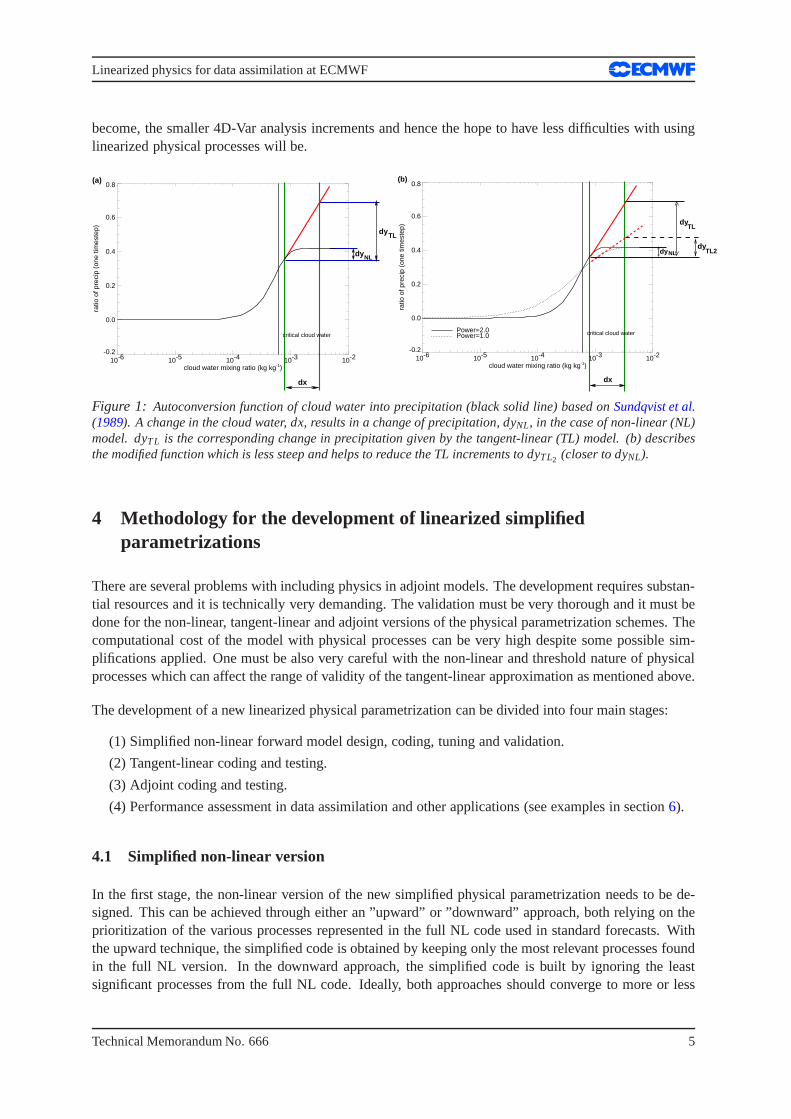
To illustrate a potential source of problem in the linearized model, the rain production function, describ-ing which portion of the cloud water is converted into precipitation, is shown in Fig.1. An increaseof cloud water mixing ratio by a small amountdx (Fig. 1a) leads to a small change in the precipitationamountdyNL in the case of the non-linear (NL) model, but to a much larger change (dyTL) in the caseof the TL model. As a possible solution, one can modify the function to make it less steep (dotted lineon Fig. 1b ). In this case, the resulting TL increment will be significantly smaller (dyTL2). However,the required modification can be substantial and it can deteriorate the overall quality of the physicalparametrization itself. Therefore one must always be careful to keep the right balance between linearityand realism of the parametrization schemes. In the future, the better the non-linear forecast model will



become, the smaller 4D-Var analysis increments and hence the hope to have less difficulties with usinglinearized physical processes will be.

10-6 10-5 10-4 10-3 10-2

cloud water mixing ratio (kg kg-1)

-0.2

0.0

0.2

0.4

0.6

0.8

ratio

of p

reci

p (o

ne ti

mes

tep)

critical cloud water

dx

(a)

dy NL

dy TL

10-6 10-5 10-4 10-3 10-2

cloud water mixing ratio (kg kg-1)

-0.2

0.0

0.2

0.4

0.6

0.8

ratio

of p

reci

p (o

ne ti

mes

tep)

critical cloud waterPower=1.0Power=2.0

dx

(b)

dyTL2

dy

NL

TL

dy

Figure 1: Autoconversion function of cloud water into precipitation(black solid line) based onSundqvist et al.(1989). A change in the cloud water, dx, results in a change of precipitation, dyNL, in the case of non-linear (NL)model. dyTL is the corresponding change in precipitation given by the tangent-linear (TL) model. (b) describesthe modified function which is less steep and helps to reduce the TL increments to dyTL2 (closer to dyNL).

4 Methodology for the development of linearized simplifiedparametrizations

There are several problems with including physics in adjoint models. The development requires substan-tial resources and it is technically very demanding. The validation must be very thorough and it must bedone for the non-linear, tangent-linear and adjoint versions of the physical parametrization schemes. Thecomputational cost of the model with physical processes canbe very high despite some possible sim-plifications applied. One must be also very careful with the non-linear and threshold nature of physicalprocesses which can affect the range of validity of the tangent-linear approximation as mentioned above.

The development of a new linearized physical parametrization can be divided into four main stages:

(1) Simplified non-linear forward model design, coding, tuning and validation.

(2) Tangent-linear coding and testing.

(3) Adjoint coding and testing.

(4) Performance assessment in data assimilation and other applications (see examples in section6).

4.1 Simplified non-linear version

In the first stage, the non-linear version of the new simplified physical parametrization needs to be de-signed. This can be achieved through either an ”upward” or ”downward” approach, both relying on theprioritization of the various processes represented in thefull NL code used in standard forecasts. Withthe upward technique, the simplified code is obtained by keeping only the most relevant processes foundin the full NL version. In the downward approach, the simplified code is built by ignoring the leastsignificant processes from the full NL code. Ideally, both approaches should converge to more or less



similar simplified codes, which should be computationally cheaper than the full NL code, and containfewer discontinuities but are still able to provide realistic forecasts. Once the simplified code has beenwritten, it is thus necessary to tune and validate it in traditional forecasts over periods at least equal to themaximum length of the expected applications. At ECMWF for instance, this period corresponds to 12hours for 4D-Var DA or to 24 hours for singular vector computations involved in the ensemble predictionsystem. It is particularly crucial to ensure that the new simplified NL code does not depart too much fromits full NL counterpart over this period of time. Verification in much longer integrations (up to climatetimescales), although not essential, is also recommended to make sure that the new simplified scheme isstable and behaves reasonably well.

4.2 Linearization techniques

Once the NL version of the simplified scheme is deemed adequate, efforts are devoted to the develop-ment of the TL code, first, and then of the AD code. In practice,linearization can be achieved usingeither a manual line-by-line approach or an automatic coding software (e.g.Giering and Kaminski 1998,Araya-Polo and Hascoet 2004). However attractive automatic coding may sound, the manual techniqueis usually more suitable as soon as one has to deal with the large amounts of complex code used in modernNWP systems. Until now, in our own experience, the code produced through automatic differentiationand adjointing often turned out to be computationally very expensive (no optimization) and sometimesnot bug-free. This is the reason why so far only manual line-by-line TL and AD coding has been appliedto derive and update ECMWF’s full set of linearized physicalparametrizations. In the future this strategymight be revisited if automatic softwares become more efficient and reliable.

4.3 Tangent-linear version

An estimation of sensitivity of model output with respect toinput required by many studies can beefficiently done by using the adjoint. For atmospheric models evolving in time, this backward integrationrequires to have the tangent linear model acting forward in time. To build the TL model, the linearizationis performed with respect to the local tangent of the model trajectory.

If M is the model describing the time evolution of the model statex as:

x(ti+1) = M[x(ti)] (4)

then the time evolution of a small perturbationδx can be estimated to the first order approximating bythe tangent linear modelM (derived from the NL modelM):

δx(ti+1) = M [x(ti)]δx(ti)

δx(ti+1) =∂M[x(ti)]

∂xδx(ti) (5)

The verification of the correctness of the TL model is first performed through the classical Taylor for-mula:

limλ→0

M(x+ λδx)−M(x)

M(λδx)= 1 (6)

This examination of asymptotic behaviour, using perturbations the size of which becomes infinitesimallysmall, is performed to check the numerical correctness of the TL code.



For practical applications, it is also important to investigate the accuracy of TL models for finite-amplitude perturbations (typically perturbations of the size of analysis increments). The results fromapplications of tangent-linear and adjoint models are onlyuseful when the linearized approximation isvalid for such perturbations. Therefore, for the validation of the tangent-linear approximation, the accu-racy of the linearization of a parametrization scheme is studied with respect to pairs of non-linear results.The difference between two non-linear integrations (one starting from a background field,xb, and theother from an analysis,xa) run with the full NL model,M, is compared to time evolution of the anal-ysis increments (xa − xb) obtained by integrating the TL model,M , with the trajectory taken from thebackground field.

For a quantitative evaluation of the impact of linearized schemes, their relative importance is evaluatedusing mean absolute errors between tangent-linear and non-linear perturbations as:

ε =∣

∣

∣M(xa−xb)−

[

M(xa)−M(xb)]

∣

∣

∣(7)

As a reference for the comparisons, an absolute mean error for the TL model without physics,εre f , istaken. Ifεexp is defined as the absolute mean error of the TL model with the different physical schemesincluded, then an improvement coming from the inclusion of more physics in the TL model is expressedasεexp< εre f . The relative errors,rer, and relative improvements,η , are also computed as:

rer =

∣

∣

∣M(xa−xb)−

[

M(xa)−M(xb)]

∣

∣

∣

∣

∣

∣M(xa)−M(xb)

∣

∣

∣

(8)

η =εexp− εre f

εre f(9)

Validity tests of the tangent-linear approximations are mostly performed over the time period and at theresolution at which adjoint models will be applied in practice: resolution and time length of an inner-loop integration of 4D-Var system (e.g. 12 hours, T255 and 91vertical levels at ECMWF) or longer timeperiods for singular vectors and sensitivity applications(e.g. 24 hours at ECMWF). An example of theresults from such TL approximation assessment will be givenin section6.1.

4.4 Adjoint version

The adjoint of a linearized operator,M , is the linear operator,M ∗, such that:

∀x,∀y < M .x,y >=< x,M ∗.y > (10)

where<,> denotes the inner product andx andy are input vectors.

Besides, the adjoint modelM ∗ can provide the gradient of any objective function,J, with respect tox(ti)from the gradient of the objective function with respect tox(ti+1)

∂J∂x(ti)

= M ∗

(

∂J∂x(ti+1)

)

(11)

The integration of the AD forecast model works backward in time. One should remember that,M beingnon-linear,M as well asM ∗ depend on the particular state of the atmosphere,x, about which the lin-earization is performed. The adjoint operator, for the simplest canonical scalar product<,> (Eq. 10), isactually the transpose of the tangent linear operator,MT (not its inverse).



For the practical verification of the adjoint code, one must test the identity described in Eq. (10). Itshould be emphasized that it is absolutely essential to ensure that the TL and AD codes verify Eq. (10)to the level of machine precision, even when vectorsx andy are global 3D atmospheric states and evenfor time integrations up to 12 or 24 hours. Note that a correctadjoint test does not imply the correctnessof tangent-linear code.

4.5 Singular vectors

Besides the verification of the numerical correctness of TL and AD versions of the model and the ex-amination of the validity of TL approximation, singular vectors can be used to find out whether the newschemes do not lead to a growth of spurious unstable modes. Such modes would indicate the existenceof strong non-linearities and threshold processes in the model and would have a negative impact on theusefulness of the linearized model.

5 ECMWF’s linearized physics package

5.1 Description

The set of ECMWF physical parametrizations used in the linearized model (called simplified or lin-earized parametrizations) comprises six different schemes for: radiation, vertical diffusion, orographicgravity wave drag, moist convection, large-scale condensation/precipitation and non-orographic grav-ity wave activity , sequentially called in this order. The current linearized physics package is thereforequite sophisticated and is believed to be the most comprehensive one used in operational global dataassimilation. Each physical parametrization scheme of this package is described below starting with dryprocesses.

5.1.1 Radiation

The radiation scheme solves the radiative transfer equation in two distinct spectral regions. The computa-tions for the longwave (LW) radiation are performed over thespectrum from 0 to 2820 cm−1 (∼ 100µmto 3.5µm). The shortwave (SW) part of the scheme integrates the fluxes over the whole shortwave spec-trum between 0.2 and 4.0µm. The scheme used for data assimilation purposes must be computationallyefficient to be called at full spatial resolution to improve the description of cloud-radiation interactionsduring the assimilation period (Janiskovaet al.2002).

The shortwave radiation scheme:

The linearized code for the SW radiation scheme has been derived from ECMWF’s original non-linearscheme developed byFouquart and Bonnel(1980) and revised byMorcrette(1991). In this scheme,previously used in the operational forecast model, the photon-path-distribution method is applied toseparate the parametrization of scattering processes fromthat of molecular absorption. UpwardF↑

sw

and downwardF↓sw fluxes at a given levelj are obtained from the reflectance and transmittance of the

atmospheric layers as

F↓sw( j) = F0

N

∏k= j

Tbot(k) (12)

F↑sw( j) = F↓

sw( j)Rtop( j −1) (13)



Computations of the transmittance at the bottom of a layer,Tbot, start at the top of atmosphere and workdownwards. Those of the reflectance at the top of the same layer, Rtop, start at the surface and workupwards. In the presence of cloud in the layer, the final fluxesare computed as a weighted average ofthe fluxes in the clear-sky and in the cloudy fractions of the column (depending on the cloud-overlapassumption).

The non-linear scheme is reasonably fast for application in4D-Var and has therefore been linearizedwithout a-priori changes (Janiskovaet al. 2002). The only modification with respect to the non-linearversion (used operationaly until June 2007; since then Rapid Radiation Transfer model for SW radiationis used -Mlawer and Clough 1997), is the use of two spectral intervals, instead of six intervals. This ismeant to reduce the computational cost.

The longwave radiation scheme:

The LW radiation scheme, used in the ECMWF full NL forecast model is the Rapid Radiation TransferModel (RRTM;Mlaweret al. 1997, Morcretteet al. 2001). The complexity of the RRTM scheme forthe LW part of the spectrum makes accurate computations expensive. In the variational assimilationframework, the older operational scheme ofMorcrette(1989) was linearized. In this scheme, the LWspectrum from 0 to 2820 cm−1 is divided into six spectral regions. The transmission functions forwater vapour and carbon dioxide over those spectral intervals are fitted using Pade approximations onnarrow-band transmissions obtained with statistical bandmodels (Morcretteet al. 1986). Integrationof the radiation transfer equation over wavenumberν within the particular spectral regions yields theupward and downward fluxes.

The inclusion of cloud effects on the LW fluxes follows the treatment discussed byWashington and Williamson(1997). The scheme first calculates upward and downward fluxes(F↑

0 (i) and F↓0 (i)) for a clear-sky atmosphere. In any cloudy layer, the schemeevaluates the fluxes

assuming a unique overcast cloud of emissivity unity, i.e.F↑n (i) andF↓

n (i) for a cloud present in thenthlayer of the atmosphere. The fluxes for the actual atmosphereare derived from a linear combination ofthe fluxes calculated in the previous steps with some cloud overlap assumption (see below) in the caseof clouds spreading over several layers. IfN is the number of model layers starting from the top ofatmosphere to the bottom,Ci the fractional cloud cover in layeri, the cloudy upwardF↑

lw and downward

F↓lw fluxes are then expressed as:

F↑lw(i) = (1−CCN,i)F

↑0 (i)+

N

∑k=i

(CCi,k+1−CCi,k)F↑k (i) (14)

F↓lw(i) = (1−CCi−1,0)F

↓0 (i)+

i−1

∑k=1

(CCi,k+1−CCi,k)F↓k (i) (15)

whereCCi, j is the cloudiness encountered between any two levelsi and j in the atmosphere computedusing the overlap assumption described below.

In the case of semi-transparent clouds, the fractional cloudiness entering the calculations is an effectivecloud cover equal to the product of the emissivity due to condensed water and gases in the layer by thehorizontal coverage of the cloud cover. This is the so calledeffective emissivity approach.

To reduce a computational cost of the linearized LW radiation for data assimilation, the scheme is notcalled at each time step. Furthermore, the transmission functions are only computed for H2O and CO2

absorbers (though the version taking into account the wholespectrum of absorbers is also coded foraerosols and other gases. The cloud effects on LW radiation are only computed up to cloud top.



Cloud overlap assumptions:

Cloud overlap assumptions must be made in atmospheric models in order to organize the cloud distribu-tion used for radiation. This is is necessary to account for the fact that clouds often do not fill the wholegrid box. The maximum-random overlap assumption (originally introduced inGeleyn and Hollingsworth1997) is used operationally (Morcrette and Jakob 2000). Adjacent cloudy layers are combined by assum-ing maximum overlap to form a contiguous cloud and discrete layers separated by clear-sky are combinedrandomly.

Cloud optical properties:

When one considers cloud-radiation interactions, it is notonly the cloud fraction or cloud volume, butalso cloud optical properties that matter. In the case of SW radiation, cloud radiative calculations de-pend on three different parameters: the optical thickness,the asymmetry factor and the single scatteringalbedo. They are derived fromFouquart(1987) for water clouds, andEbert and Curry(1992) for iceclouds. They are functions of cloud condensate and a specified effective radius.

Cloud LW optical properties are represented by the emissivity, related to the condensed water amount,and by the condensed-water mass absorption coefficient obtained fromSmith and Shi(1992) for waterclouds andEbert and Curry(1992) for ice clouds.

5.1.2 Vertical diffusion

Vertical diffusion applies to wind components, dry static energy and specific humidity. The exchangecoefficients in the planetary boundary layer and the drag coefficients in the surface layer are expressedas functions of the local Richardson number,Ri, (Louis et al.1982). They differ from the formulation ofthe operational forecast model (i.e. full non-linear scheme) where for the unstable regime (Ri < 0) theMonin-Obukhov (M-O) formulation is used, together with a K-profile approach for convectively mixedlayer in the case of unstable surface conditions. In the linearized model, the exchange coefficients arecomputed according toLouis et al. (1982). For the stable regime (Ri > 0), diffusion coefficients accord-ing to the Louis scheme are used close to the surface and above300 m, then they tend asymptoticallyto the M-O formulation. A mixed layer parametrization is also included. This is consistent with the fullnon-linear model.

Analytical expressions are generalized for the situation with different roughness lengths for heat andmomentum transfer. For any conservative variableψ (wind vector components,u and v; dry staticenergy,s; specific humidity,q), the tendency produced by vertical diffusion is

∂ψ∂ t

=1ρ

∂∂z

(

K(Ri)∂ψ∂z

)

(16)

whereρ is the air density. The exchange coefficientK for heat and momentum transfer is given by

K = l2

∥

∥

∥

∥

∂U∂z

∥

∥

∥

∥

f (Ri) (17)

whereU is the wind vector andf (Ri) represents the coefficient accounting for the dependence ofverticalturbulent diffusion on the local Richardson number, eithercomputed according toLouis et al. (1982),fL(Ri), or to the Monin-Obukhov formulation,fMO(Ri). l is the mixing length profile based on theformulation ofBlackadar(1962) with a reduction in the free atmosphere.



A continuous transition between Louis coefficients near thesurface to about 300 m and M-O coefficientsabove is computed as

1

l√

f (Ri)=

1

κz√

fL(Ri)+

1

λ√

fMO(Ri)(18)

whereκ is the Von Karman’s constant,z is the height andλ is the asymptotic mixing length.

To parametrize turbulent fluxes at the surface, the drag coefficient, Cs f, (i.e. the exchange coefficientbetween the surface and the lowest model level) is computed as

Cs f = gs f(Ri) CN (19)

whereCN is the neutral drag coefficient, which is a function of the roughness length, andgs f(Ri) is afunction of the local Richardson number. Different formulations ofCN andgs f(Ri) are used for momen-tum and heat, according toLouis et al. (1982).

Regularization:

In earlier versions of the model, perturbations of the exchange coefficients were simply neglected (K′ =0), in order to prevent spurious unstable perturbations from growing in the linearized version of thescheme (Mahfouf 1999). Later, some regularization of exchange coefficients was introduced at uppermodel levels to allow partial perturbations of these coefficients. This consists in the perturbations beingmore significantly reduced around the neutral state (i.e.Ri close to zero) where both the function ofRiitself and its derivative exhibit a significant rate of change. The reduction is eased exponentially awayfrom the neutral state.

5.1.3 Subgrid scale orographic effects

Only the low-level blocking part of the operational non-linear scheme developed byLott and Miller(1997) is taken into account in TL and AD calculations. The deflection of the low-level flow aroundorographic obstacles is supposed to occur below an altitudeZblk such that

∫ 3µ

Zblk

N|U|

dz≥ Hncrit (20)

whereHncrit is a critical non-dimensional mountain height,µ is the standard deviation of subgrid-scaleorography andN is the Brunt-Vaisala frequency.

The deceleration of wind due to low-level blocking is given by

(

∂U∂ t

)

blk= −Cdmax

(

2−1r,0

)

σ2µ

√

Zblk −zz+ µ

(Bcos2α +Csin2 α)U|U|

2(21)

whereCd is the low-level drag coefficient,σ is the mean slope of the subgrid-scale orography, andαis the angle between the low-level wind and the principal axis of orography. r is determined asr =(cos2α + γ sin2α)/(γ cos2α + sin2α), whereγ is the anisotropy of the subgrid-scale orography. ThefunctionsB, C are written as (Phillips 1984)

B = 1−0.18γ −0.04γ2 and C = 0.48γ +0.3γ2.

The final wind tendency produced by the low-level drag parametrization is then obtained from the fol-lowing partially implicit discretization of Eq. (21)

(

∂U∂ t

)

blk=

Un+1−Un

∆t= −A|Un|Un+1 = −

β1+ β

Un

∆t(22)



whereβ = A|Un|∆t andUn+1 = Un/(1+ β ).

5.1.4 Non-orographic gravity wave drag

The tangent-linear and adjoint versions of the non-linear scheme for non-orographic gravity waves (indetails described byOrr et al. 2010) were developed in order to reduce discrepancies between the fullNL and linearized versions of the model, especially in the stratosphere. The parametrization schemeused in the NL model is based onScinocca(2003). This is a spectral scheme that follows from theWarner and McIntyre(1996) scheme representing the three basic mechanisms that are conservative prop-agation, critical level filtering, and non-linear dissipation. Since the full nonhydrostatic and rotationalwave dynamics considered byWarner and McIntyre(1996) is too costly for operational models, onlyhydrostatic and non-rotational wave dynamics are employed.

The dispersion relation for a hydrostatic gravity wave in the absence of rotation is

m2 =k2N2

ω2 =N2

c2 (23)

wherek, m are horizontal and vertical wavenumbers, whileω = ω −kU andc = c−U are the intrinsicfrequency and phase speed (withc being the ground based phase speed andU the background wind speedin the direction of propagation), respectively.

The launch spectrum, which is globally uniform and constant, is given by the total wave energy per unitmass in each azimuth angleφ following Fritts and VanZandt(1993) as

E(m, ω ,φ) = B( m

m∗

)s N2ω−d

1−(

mm∗

)s+3 (24)

whereB, s andd are constants, andm∗ = 2πL is a transitional wavelength. Instead of the total waveenergyE(m, ω ,φ), the momentum flux spectral densityρF(m, ˜ω ,φ ) is required. This is obtained throughthe group velocity rule. In order to have the momentum flux conserved in the absence of dissipativeprocesses as the spectrum propagates vertically through height-varying background wind and buoyancyfrequency, the coordinate framework(k,ω) is used instead of(m, ω) as shown inScinocca(2003).

The dissipative mechanisms applied to the wave field in each azimuthal direction and on each model levelare critical level filtering and non-linear dissipation. After application of them, the resulting momentumflux profiles are used to derive the net eastwardρFE and northwardρFN fluxes. The tendencies for the(u, v) wind components are then given by the divergence of those fluxes obtained through summation ofthe total momentum flux (i.e. integrated over all phase speedbins) in each azimuthφi projected onto theeast and north directions, respectively:

∂u∂ t

= g∂ (ρFE)

∂ p(25)

∂v∂ t

= g∂ (ρFN)

∂ p(26)

whereg is the gravitational acceleration andp is pressure.

Regularization:

In order to eliminate the spurious noise in TL computations caused by the introduction of this scheme,it was necessary to implement some regularizations. These include rewriting buoyancy frequency (N)



computations in the NL scheme in height coordinates insteadof pressure coordinates (as used in theoriginal code) and setting increments for momentum flux in the last three spectral elements (high phasespeed) of the launch spectrum to zero.

5.1.5 Moist convection

The original version of the simplified mass-flux convection scheme currently used in the minimization of4D-Var is described inLopez and Moreau(2005). Through time, the original scheme has been updatedso as to gradually converge towards the full convection scheme used in high-resolution 10-day forecasts(Bechtoldet al.2008). The transport of tracers by convection is also implemented.

The physical tendencies produced by convection on any conservative variableψ (dry static energy, windcomponents, specific humidity, cloud liquid water) can be written in mass-flux form followingBetts(1997)

∂ψ∂ t

=1ρ

[

(Mu +Md)∂ψ∂z

+Du(ψu−ψ)+Dd(ψd−ψ)

]

(27)

The first term on the right hand side represents the compensating subsidence induced by cumulus con-vection on the environment through the mass flux,M. The other terms account for the detrainment ofcloud properties in the environment with a detrainment rate, D. Subscriptsu andd refer to the updraughtsand downdraughts properties, respectively. Evaporation of cloud water and precipitation should also beadded in Eq. (27) for dry static energy,s= cpT +gz, and specific humidity.

Equations for updraught and downdraught:

The equations describing the evolution with height of the convective updraught and downdraught massfluxes,Mu andMd, respectively, are

∂Mu

∂z= (εu−δu)Mu (28)

∂Md

∂z= −(εd−δd)Md (29)

whereε and δ respectively denote the entrainment and detrainment rates. A second set of equationsis used to describe the evolution with height of any other characteristic,ψ , of the updraught or down-draught, namely

∂ψu

∂z= −εu(ψu−ψ) (30)

∂ψd

∂z= εd(ψd−ψ) (31)

whereψ is the value ofψ in the large-scale environment.

In practice, Eqs. (28)-(29) are solved in terms ofµ = M/Mbaseu , whereMbase

u is the mass flux at cloudbase (determined from the closure assumption as described further down).

Triggering of moist convection:

The determination of the occurrence of moist convection in the model is based on whether a positivelybuoyant test parcel starting at each model level (iteratively from the surface and upwards) can rise highenough to produce a convective cloud and possibly precipitation. For an updraught starting from the



lowest model level, its initial temperature and moisture departures with respect to the environment and itsinitial vertical velocity depend on surface sensible and latent heat fluxes, followingJakob and Siebesma(2003). When starting from higher model levels, the ascent is initially set to 1 m s−1 and its initialthermodynamic characteristics are assumed to be representative of a few hundred metre deep mixed-layer, with typical excesses of 0.2 K for temperature and 1×10−4 kg kg−1 for moisture. A 200 hPathreshold for cloud depth is prescribed to distinguish between shallow and deep convection. Mid-levelconvection is treated as deep convection.

Entrainment and detrainment:

Entrainment rate in the updraught (εu) is split into turbulent and organized components, which are bothmodulated by humidity conditions in the environment. Detrainment in the updraught (δu) is assumedto occur inside the convective cloud only where the updraught vertical gradient of kinetic energy andbuoyancy are negative, that is usually in the upper part of the convective cloud.

Entrainment in downdraughts (εd) is assumed to occur only between the level of free sinking and thetop of the 60 hPa atmospheric layer just above the surface. Inside this layer, it is set to a constant value.Detrainment (δd) is defined such as to ensure a downward linear decrease of downdraught mass flux tozero at the surface.

Precipitation processes:

The formation of precipitation from the cloud water contained in the updraught is parametrized accordingto Sundqvistet al. (1989) and a simple representation of precipitation evaporationis included. Precip-itation formed from cloud liquid water at temperatures below the freezing point is assumed to freezeinstantly, which affects the dry static energy tendency.

Closure assumptions:

One needs to formulate so-called closure assumptions to relate the convective updraught mass-flux atcloud base,Mbase

u , to quantities that are explicitly resolved by the model. For deep convection, theclosure is based on the balance between the convective available potential energy in the subgrid-scaleupdraught and the total heat release in the resolved larger-scale environment. The cloud base mass fluxis expressed as the ratio of the latter two quantities, modulated with an adjustment timescale. Thistimescale depends on the updraught vertical velocity averaged over its depth and on spectral truncation.For shallow convection, the closure assumption links the moist energy excess at cloud base to the moistenergy convergence inside the sub-cloud layer. The ratio ofthese two quantities yields the cloud basemass flux for shallow convection.

Regularization:

Various regularizations need to be applied in the TL and AD code of the convection scheme to avoidspurious instabilities. These include reducing or settingto zero the perturbations of some terms thatdirectly depend on the updraught vertical velocity as well as reducing updraught buoyancy and cloudbase mass flux perturbations.

5.1.6 Large-scale condensation and precipitation

The original version of the simplified diagnostic large-scale clouds and precipitation scheme currentlyused in the minimization of 4D-Var is described inTompkins and Janiskova(2004). Only a summary of



its main features is given here.

The physical tendencies of temperature and specific humidity produced by moist processes on the large-scale can be written as

∂q∂ t

= −Cce+Eprec+Dconv (32)

∂T∂ t

= L(Cce−Eprec−Dconv)+L f (Frain−Msnow) (33)

whereCce denotes large-scale condensation/evaporation,Eprec is the moistening due to the evaporationof precipitation andDconv is the detrainment of cloud water from convective clouds.Frain and Msnow

correspond to the freezing of rain and melting of snow, respectively. L andLf are the latent heats ofvaporisation/sublimation and fusion, respectively.

Condensation:

The subgrid-scale variability of humidity is assumed to be represented by a uniform distribution. Thisallows the estimation of the stratiform cloud fraction,Cstrat, and cloud condensate amount,qstrat

c , fromthe grid-box relative humidity,RH, as

Cstrat = 1−

√

1−RH1−RHcrit −κ(RH−RHcrit)

(34)

qstratc = qsatC

2strat

{

κ(1−RH)+ (1−κ)(1−RHcrit)}

(35)

whereqsat is the saturation specific humidity. The critical relative humidity threshold,RHcrit, and thecoefficientκ are specified as inTompkins and Janiskova(2004). A simple diagnostic partitioning basedon temperature is used to separate cloud condensate into liquid and ice.

The impact of convective activity on large-scale clouds, which is particularly important in the tropics andmid-latitude summers, is accounted for through the detrainment rate produced by the convection scheme.This detrainment term is used to compute the additional cloud cover and cloud condensate resulting fromconvection (i.e. convection called before condensation).

Precipitation processes:

The formation of precipitation from cloud condensate,qc, is parametrized according toSundqvistet al.(1989), but the Bergeron-Findeisen mechanism and collection processes are currently disregarded. Pre-cipitation formed from cloud liquid water at temperatures below the freezing point is assumed to freezeinstantly, which corresponds to termFrain in Eq. (33). On the other hand, precipitation evaporation is es-timated from the overlap of precipitation with the uniformly distributed subgrid fluctuations of humidityinside the clear-sky fraction of the grid box.

Regularization:

Perturbations ofCstrat were found to cause spurious instabilities in TL and AD integrations and aretherefore artificially reduced according to the value ofCstrat in the trajectory. A reduction of perturbationsin the autoconversion of cloud condensate to precipitationis also needed.



5.2 A few remarks

The set of physical parametrization schemes developed for the ECMWF linearized model was describedin section5.1. Although there are some simplifications and regularizations applied in the differentparametrization schemes, the whole package is comprehensive and its non-linear form is able to pro-vide 2-3 days forecasts that show a degree of realism which does not depart too much from that of thenon-linear physics. Different levels of simplification of the schemes have been driven either by the re-quirement to decrease computational cost for operational applications or the necessity to avoid unrealisticperturbations in the linearized version of the scheme. The applied regularizations and simplifications al-low global integrations of the linearized model with elaborated physical parametrization schemes evenup to 48 hours without producing spurious noise.

Overall, the presented package is a result of compromise between realism, linearity and computationalcost while at the same time the level of complexity for the parametrization schemes is also influencedby the required applications. It is a constant challenge to maintain the best tradeoff between all thoserequirements.

5.3 Benefits of regularization

The validity of the tangent-linear approximation can be highly degraded due to the non-linear and dis-continuous nature of physical processes (see section3.2). If the derivatives of model outputs with respectto the model state variables become very large, the linearization will become useless.

As an illustration of how strong nonlinearities can lead to erroneous behaviour of the tangent linearmodel, Fig.2b shows the evolution of zonal wind increments at the model level around 700 hPa whenusing the TL model without any regularization in the cloud parametrization scheme. When comparedto the finite differences (differences between two non-linear integrations) in Fig.2a, one can notice thatstrong spurious noise develops in the tangent linear model.This noise comes from the autoconversionfunction (Fig. 1) describing the conversion of cloud water to precipitation. When regularization isapplied to this function, TL increments (Fig.2c) agree well with the finite differences (Fig.2a).

(a) FD: 20010315 12UTC t+12 Level 44 u-velocity

-12

-8

-4

-2

-1

-0.50.5

1

2

4

8

12(b) TL_nonreg: 20010315 12UTC t+12 Level 44 u-velocity

-12 10

-8 10

-4 10

-2 10

-1 10

-0.5 100.5 10

1 10

2 10

4 10

8 10

12 10

5

5

5

5

5

5

5

5

5

5

5

5

(c) TL_reg: 20010315 12UTC t+12 Level 44 u-velocity

-12

-8

-4

-2

-1

-0.50.5

1

2

4

8

12

Figure 2: Zonal wind increments around 700 hPa after 12-hour evolution: (a) finite-differences (FD), (b)tangent-linear (TL) model without any regularization and (c) TL model with applied regularization in the cloudparametrization scheme.



6 Performance of the linearized physics

6.1 TL approximation

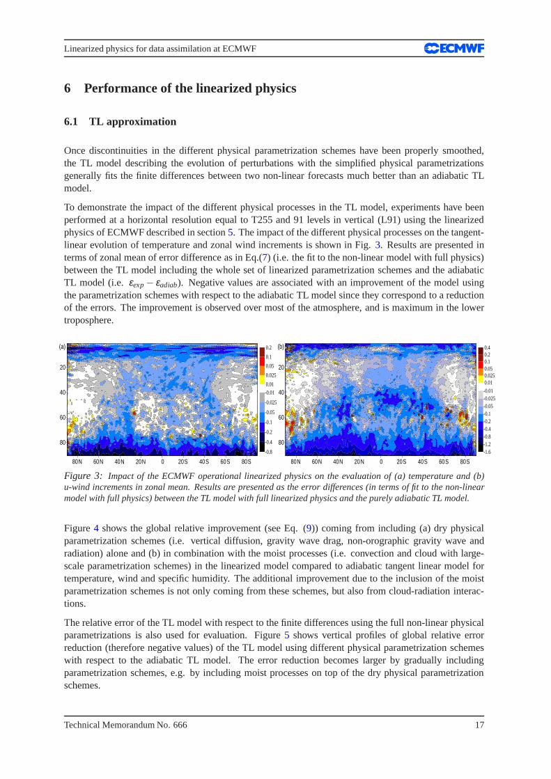
Once discontinuities in the different physical parametrization schemes have been properly smoothed,the TL model describing the evolution of perturbations withthe simplified physical parametrizationsgenerally fits the finite differences between two non-linearforecasts much better than an adiabatic TLmodel.

To demonstrate the impact of the different physical processes in the TL model, experiments have beenperformed at a horizontal resolution equal to T255 and 91 levels in vertical (L91) using the linearizedphysics of ECMWF described in section5. The impact of the different physical processes on the tangent-linear evolution of temperature and zonal wind increments is shown in Fig.3. Results are presented interms of zonal mean of error difference as in Eq.(7) (i.e. the fit to the non-linear model with full physics)between the TL model including the whole set of linearized parametrization schemes and the adiabaticTL model (i.e. εexp− εadiab). Negative values are associated with an improvement of themodel usingthe parametrization schemes with respect to the adiabatic TL model since they correspond to a reductionof the errors. The improvement is observed over most of the atmosphere, and is maximum in the lowertroposphere.

80N 60N 40N 20N 0 20S 40S 60S 80S

80

60

40

20

(a)

-0.8

-0.4

-0.2

-0.1

-0.05

-0.025

-0.01

0.01

0.025

0.05

0.1

0.2

80N 60N 40N 20N 0 20S 40S 60S 80S

80

60

40

20

(b)

-1.6-1.2-0.8-0.4-0.2-0.1-0.05-0.025-0.01

0.010.0250.050.10.20.4

Figure 3: Impact of the ECMWF operational linearized physics on the evaluation of (a) temperature and (b)u-wind increments in zonal mean. Results are presented as the error differences (in terms of fit to the non-linearmodel with full physics) between the TL model with full linearized physics and the purely adiabatic TL model.

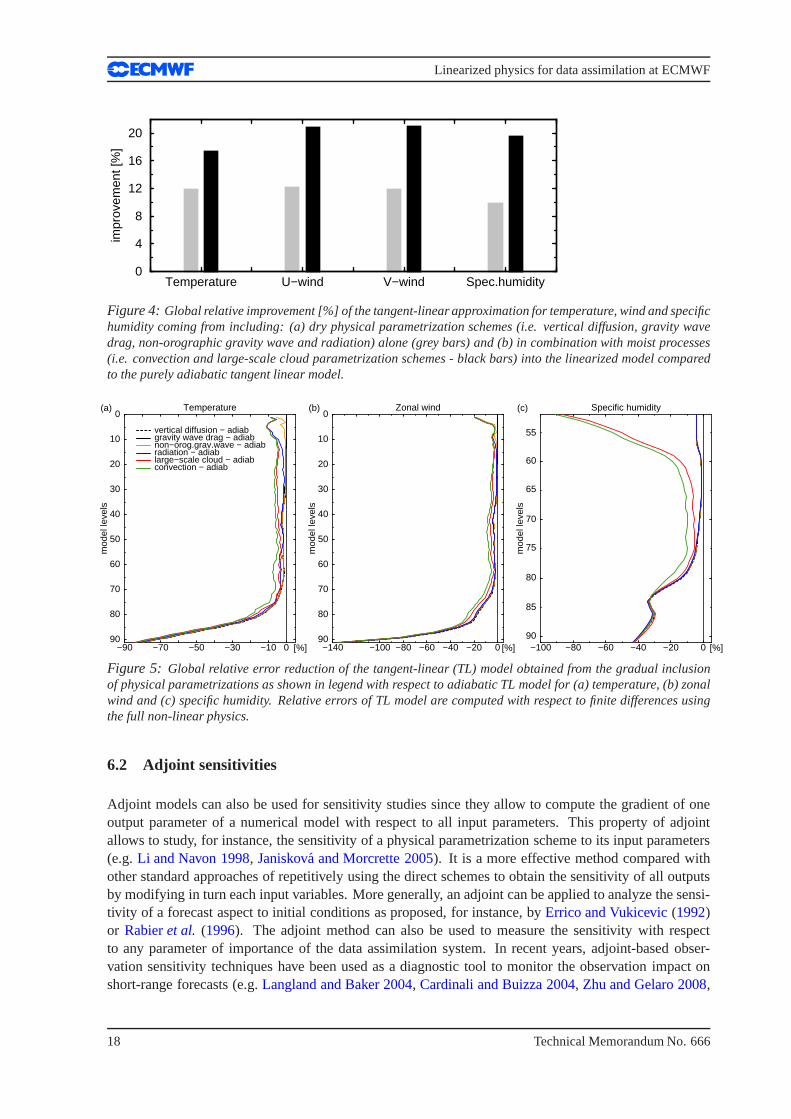
Figure4 shows the global relative improvement (see Eq. (9)) coming from including (a) dry physicalparametrization schemes (i.e. vertical diffusion, gravity wave drag, non-orographic gravity wave andradiation) alone and (b) in combination with the moist processes (i.e. convection and cloud with large-scale parametrization schemes) in the linearized model compared to adiabatic tangent linear model fortemperature, wind and specific humidity. The additional improvement due to the inclusion of the moistparametrization schemes is not only coming from these schemes, but also from cloud-radiation interac-tions.

The relative error of the TL model with respect to the finite differences using the full non-linear physicalparametrizations is also used for evaluation. Figure5 shows vertical profiles of global relative errorreduction (therefore negative values) of the TL model usingdifferent physical parametrization schemeswith respect to the adiabatic TL model. The error reduction becomes larger by gradually includingparametrization schemes, e.g. by including moist processes on top of the dry physical parametrizationschemes.



Temperature U−wind V−wind Spec.humidity0

4

8

12

16

20

impr

ovem

ent [

%]

Figure 4: Global relative improvement [%] of the tangent-linear approximation for temperature, wind and specifichumidity coming from including: (a) dry physical parametrization schemes (i.e. vertical diffusion, gravity wavedrag, non-orographic gravity wave and radiation) alone (grey bars) and (b) in combination with moist processes(i.e. convection and large-scale cloud parametrization schemes - black bars) into the linearized model comparedto the purely adiabatic tangent linear model.

−90 −70 −50 −30 −10 0 [%]

(a)0

10

20

30

40

50

60

70

80

90

mod

el le

vels

Temperature

vertical diffusion − adiabgravity wave drag − adiabnon−orog.grav.wave − adiabradiation − adiablarge−scale cloud − adiabconvection − adiab

−140 −100 −80 −60 −40 −20 0 [%]

(b)0

10

20

30

40

50

60

70

80

90

mod

el le

vels

Zonal wind

−100 −80 −60 −40 −20 0 [%]

(c)

55

60

65

70

75

80

85

90

mod

el le

vels

Specific humidity

Figure 5: Global relative error reduction of the tangent-linear (TL)model obtained from the gradual inclusionof physical parametrizations as shown in legend with respect to adiabatic TL model for (a) temperature, (b) zonalwind and (c) specific humidity. Relative errors of TL model are computed with respect to finite differences usingthe full non-linear physics.

6.2 Adjoint sensitivities

Adjoint models can also be used for sensitivity studies since they allow to compute the gradient of oneoutput parameter of a numerical model with respect to all input parameters. This property of adjointallows to study, for instance, the sensitivity of a physicalparametrization scheme to its input parameters(e.g.Li and Navon 1998, Janiskova and Morcrette 2005). It is a more effective method compared withother standard approaches of repetitively using the directschemes to obtain the sensitivity of all outputsby modifying in turn each input variables. More generally, an adjoint can be applied to analyze the sensi-tivity of a forecast aspect to initial conditions as proposed, for instance, byErrico and Vukicevic(1992)or Rabieret al. (1996). The adjoint method can also be used to measure the sensitivity with respectto any parameter of importance of the data assimilation system. In recent years, adjoint-based obser-vation sensitivity techniques have been used as a diagnostic tool to monitor the observation impact onshort-range forecasts (e.g.Langland and Baker 2004, Cardinali and Buizza 2004, Zhu and Gelaro 2008,



Cardinali 2009). Such technique is restricted by the tangent-linear assumption and its validity. The betterthe tangent-linear approximation, the more realistic and useful the sensitivity patterns. Results obtainedthrough the adjoint integration when using a too simplified adjoint model with large inaccuracies oradjoint models without a proper treatment of nonlinearities and discontinuities, can be incorrect.

The adjoint(FT) of the linear operatorF can provide the gradient of any objective function,J, withrespect tox (input variables) given the gradient ofJ with respect toy (output variables) as:

∂J∂x

= FT .∂J∂y

(36)

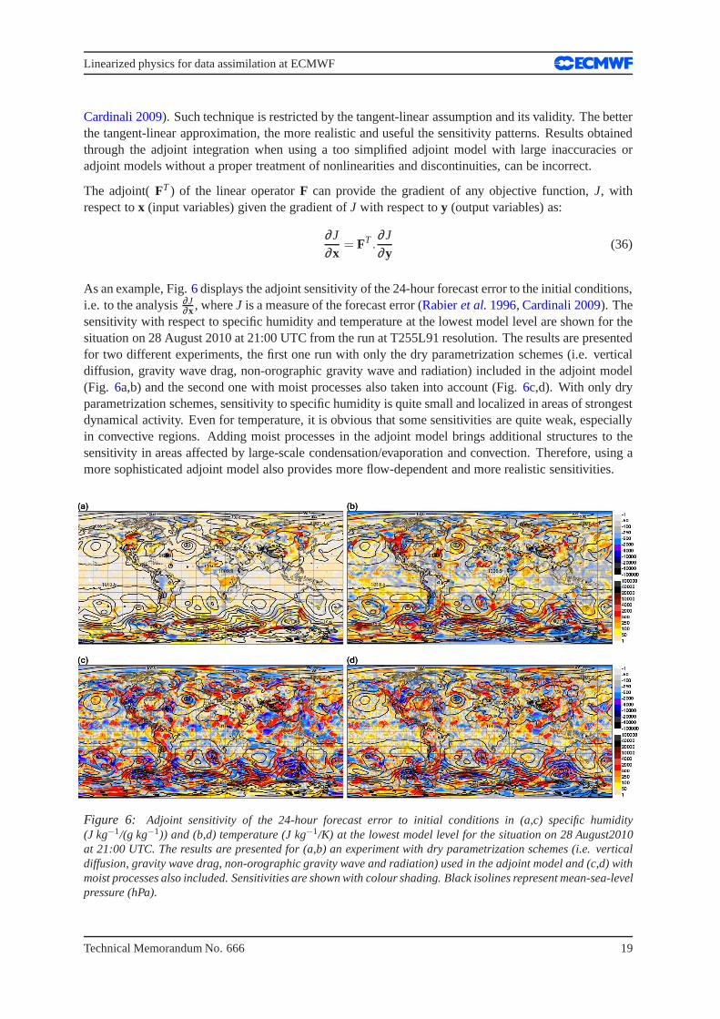
As an example, Fig.6displays the adjoint sensitivity of the 24-hour forecast error to the initial conditions,i.e. to the analysis∂J

∂x , whereJ is a measure of the forecast error (Rabieret al.1996, Cardinali 2009). Thesensitivity with respect to specific humidity and temperature at the lowest model level are shown for thesituation on 28 August 2010 at 21:00 UTC from the run at T255L91 resolution. The results are presentedfor two different experiments, the first one run with only thedry parametrization schemes (i.e. verticaldiffusion, gravity wave drag, non-orographic gravity waveand radiation) included in the adjoint model(Fig. 6a,b) and the second one with moist processes also taken into account (Fig.6c,d). With only dryparametrization schemes, sensitivity to specific humidityis quite small and localized in areas of strongestdynamical activity. Even for temperature, it is obvious that some sensitivities are quite weak, especiallyin convective regions. Adding moist processes in the adjoint model brings additional structures to thesensitivity in areas affected by large-scale condensation/evaporation and convection. Therefore, using amore sophisticated adjoint model also provides more flow-dependent and more realistic sensitivities.

Figure 6: Adjoint sensitivity of the 24-hour forecast error to initial conditions in (a,c) specific humidity(J kg−1/(g kg−1)) and (b,d) temperature (J kg−1/K) at the lowest model level for the situation on 28 August2010at 21:00 UTC. The results are presented for (a,b) an experiment with dry parametrization schemes (i.e. verticaldiffusion, gravity wave drag, non-orographic gravity waveand radiation) used in the adjoint model and (c,d) withmoist processes also included. Sensitivities are shown with colour shading. Black isolines represent mean-sea-levelpressure (hPa).



990 995

1000

1000

1000

1000

1005

1005

1005

1010

1010

1010

1015

1015

1020

1020

1025

1025

40°N

50°N

60°N50°W

50°W

40°W

40°W

30°W

30°W

20°W

20°W

10°W

10°W

0°

0° 10°E

10°E

20°E

20°E

Mean precipitation inside target box = 15.81 mm/daymm/day

0.1

1

5

10

20

50

100

Figure 7: Map of 3-hour precipitation accumula-tions ending at 0000 UTC 10 February 2009 and usedfor computing the precipitation cost function insidethe target black box over northwestern Europe. Greyshading shows precipitation (in mm day−1), whileblack isolines of mean-sea-level pressure are alsoplotted (in hPa).

995

995

995

995

1000

1000

1000

1000

1005

1005

1005

1010

1010

1010

1010

10151015

1020

1020

1020

-3-2

-1

-1

1

1

1

2

4.9

-5.1

40°N

50°N

60°N50°W

50°W

40°W

40°W

30°W

30°W

20°W

20°W

10°W

10°W

0°

0° 10°E

10°E

20°E

20°E

K

220

225

230

235

240

245

250

255

260

263.2

Figure 8: Adjoint sensitivities of the precipitationcost function defined over the black box (see Fig.7)with respect to 500-hPa temperature at 0000 UTC 9February 2009, i.e. with a lead time of 24 hours. Sen-sitivities are shown with white isolines (solid for pos-itive, dash for negative) and are expressed in unitsof 10−4 (mm day−1) K−1. The background 500 hPatemperature field valid at 0000 UTC 9 February 2009is displayed using grey shading and black isolines ofmean-sea-level pressure are also plotted (in hPa).

Another example of adjoint sensitivity computations usingthe adjoint version of the linearized physicspackage is given here, where the cost function was defined as the 3-hour precipitation averaged overthe core of a mid-latitude winter storm over northwestern Europe. One should emphasize that this kindof computation is only possible if the adjoint of moist physics parametrizations is available. Figure7shows the field of 3-hour precipitation accumulation used for the evaluation of the precipitation costfunction inside the black box at 0000 UTC 10 February 2009. Asan illustration, Fig.8 displays theadjoint sensitivities of the precipitation cost function with respect to 500 hPa temperature at 0000 UTC9 February 2009 (i.e. 24 hours beforehand and computed at T159L91 resolution). In other words, Fig.8 points out the regions where temperature ought to be modifiedin order to change precipitation insidethe target box, 24 hours later. In Fig.8, the region of maximum sensitivity is found in the vicinity of thecold front associated with the 990 hPa low pressure system located at 19◦W/47◦N. The dipolar patternof sensitivities indicates that a strengthening of the cross-frontal temperature gradient would result in aprecipitation increase inside the black box, 24 hours later.

Of course, it would also be possible to plot sensitivities with respect to moisture, wind and surfacepressure fields for this case (not shown). In fact, sensitivities can be computed with respect to anyvariable which is part of the control vector of the adjoint model. However, one should also keep in mindthat the relevance and usefulness of adjoint sensitivitiescan be limited by the degradation of the linearityassumption over time.

6.3 Data assimilation

Experiments have been performed over July-September 2011 in order to compare two versions of theECMWF 4D-Var system at resolution T5113L91: the first one including the linearized physics described

3T511 corresponding approximately to 40 km



above and the second one without it. Actually, in the versionwithout the described linearized physics, asimple linear vertical diffusion (dry and acting mainly close to surface) and surface drag scheme (Buizza1994) had to be used to avoid strong wind increments close to the surface. Precipitation and cloud relatedobservations have not been taken assimilated in order to usethe same type of observations in both ex-periments. Indeed, without the linearized moist physics in4D-Var, cloud and precipitation observationscannot be assimilated since no observation equivalent can be produced from the model.

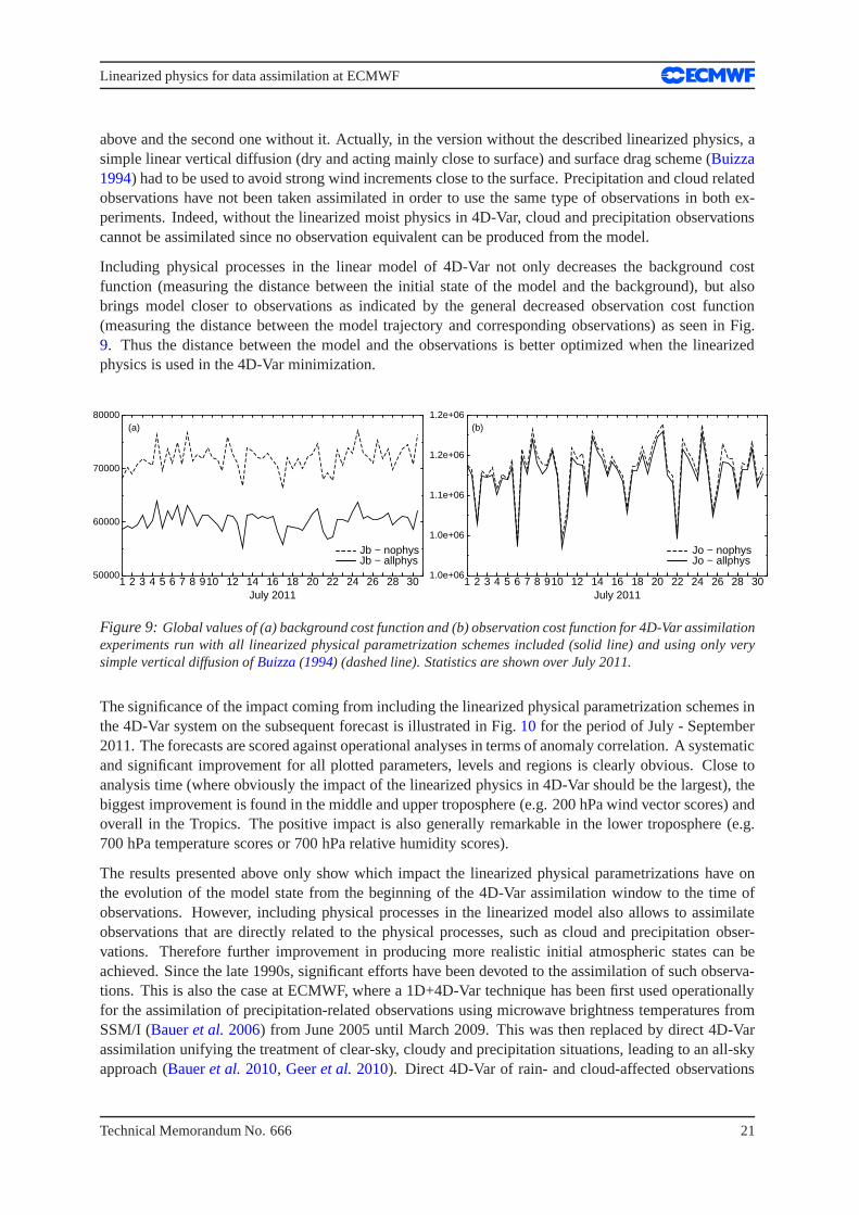
Including physical processes in the linear model of 4D-Var not only decreases the background costfunction (measuring the distance between the initial stateof the model and the background), but alsobrings model closer to observations as indicated by the general decreased observation cost function(measuring the distance between the model trajectory and corresponding observations) as seen in Fig.9. Thus the distance between the model and the observations isbetter optimized when the linearizedphysics is used in the 4D-Var minimization.

1 2 3 4 5 6 7 8 910 12 14 16 18 20 22 24 26 28 30July 2011

50000

60000

70000

80000(a)

Jb − nophysJb − allphys

1 2 3 4 5 6 7 8 910 12 14 16 18 20 22 24 26 28 30July 2011

1.0e+06

1.0e+06

1.1e+06

1.2e+06

1.2e+06(b)

Jo − nophysJo − allphys

Figure 9: Global values of (a) background cost function and (b) observation cost function for 4D-Var assimilationexperiments run with all linearized physical parametrization schemes included (solid line) and using only verysimple vertical diffusion ofBuizza(1994) (dashed line). Statistics are shown over July 2011.

The significance of the impact coming from including the linearized physical parametrization schemes inthe 4D-Var system on the subsequent forecast is illustratedin Fig. 10 for the period of July - September2011. The forecasts are scored against operational analyses in terms of anomaly correlation. A systematicand significant improvement for all plotted parameters, levels and regions is clearly obvious. Close toanalysis time (where obviously the impact of the linearizedphysics in 4D-Var should be the largest), thebiggest improvement is found in the middle and upper troposphere (e.g. 200 hPa wind vector scores) andoverall in the Tropics. The positive impact is also generally remarkable in the lower troposphere (e.g.700 hPa temperature scores or 700 hPa relative humidity scores).

The results presented above only show which impact the linearized physical parametrizations have onthe evolution of the model state from the beginning of the 4D-Var assimilation window to the time ofobservations. However, including physical processes in the linearized model also allows to assimilateobservations that are directly related to the physical processes, such as cloud and precipitation obser-vations. Therefore further improvement in producing more realistic initial atmospheric states can beachieved. Since the late 1990s, significant efforts have been devoted to the assimilation of such observa-tions. This is also the case at ECMWF, where a 1D+4D-Var technique has been first used operationallyfor the assimilation of precipitation-related observations using microwave brightness temperatures fromSSM/I (Baueret al. 2006) from June 2005 until March 2009. This was then replaced by direct 4D-Varassimilation unifying the treatment of clear-sky, cloudy and precipitation situations, leading to an all-skyapproach (Baueret al. 2010, Geeret al. 2010). Direct 4D-Var of rain- and cloud-affected observations



-0.04-0.02

00.020.040.060.080.100.12

0 1 2 3 4 5 6 7 8 9 10 11Forecast Day

(a) NHem: 500hPa geopotential - Anomaly correlation

-0.04

-0.02

0

0.02

0.04

0.06

0.08

0.10

0 1 2 3 4 5 6 7 8 9 10 11Forecast Day

(b) NHem: 700hPa temperature - Anomaly correlation

-0.02

0

0.02

0.04

0.06

0.08

0.10

0.12

0 1 2 3 4 5 6 7 8 9 10 11Forecast Day

(c) NHem: 200hPa rel.humidity - Anomaly correlation

-0.05

0

0.05

0.10

0.15

0.20

0.25

0 1 2 3 4 5 6 7 8 9 10 11Forecast Day

(d) NHem: 200hPa vector wind - Anomaly correlation

-0.08-0.06-0.04-0.02

00.020.040.060.08

0 1 2 3 4 5 6 7 8 9 10 11Forecast Day

(e) SHem: 500hPa geopotential - Anomaly correlation

-0.04

-0.02

0

0.02

0.04

0.06

0.08

0 1 2 3 4 5 6 7 8 9 10 11Forecast Day

(f) SHem: 700hPa temperature - Anomaly correlation

-0.02

0

0.02

0.04

0.06

0.08

0 1 2 3 4 5 6 7 8 9 10 11Forecast Day

(g) SHem: 700hPa rel.humidity - Anomaly correlation

-0.05

0

0.05

0.10

0.15

0.20

0 1 2 3 4 5 6 7 8 9 10 11Forecast Day

(h) SHem: 200hPa vector wind - Anomaly correlation

-0.15

-0.10

-0.05

0

0.05

0.10

0.15

0 1 2 3 4 5 6 7 8 9 10 11Forecast Day

(i) Europe:500hPa geopotential - Anomaly correlation

-0.10

-0.05

0

0.05

0.10

0 1 2 3 4 5 6 7 8 9 10 11Forecast Day

(j) Europe:700hPa temperature - Anomaly correlation

-0.06-0.04-0.02

00.020.040.060.080.100.12

0 1 2 3 4 5 6 7 8 9 10 11Forecast Day

(k) Europe:700hPa rel.humidity - Anomaly correlation

-0.15

-0.10

-0.05

0

0.05

0.10

0.15

0 1 2 3 4 5 6 7 8 9 10 11Forecast Day

(l) Europe: 200hPa vector wind - Anomaly correlation

-0.04-0.02

00.020.040.060.080.100.120.14

0 1 2 3 4 5 6 7 8 9 10 11Forecast Day

(m) Tropics:700hPa temperature - Anomaly correlation

-0.020

0.020.040.060.080.100.120.140.16

0 1 2 3 4 5 6 7 8 9 10 11Forecast Day

(n) Tropics:700hPa rel.humidity - Anomaly correlation

-0.05

0

0.05

0.10

0.15

0.20

0.25

0.30

0 1 2 3 4 5 6 7 8 9 10 11Forecast Day

(o) Tropics:200hPa vector wind - Anomaly correlation

Figure 10: Relative impact from the inclusion of the linearized physical parametrization schemes in ECMWF’s4D-Var system. Forecast scores against operational analysis are shown in terms of anomaly correlations for rangesup to 10 days. Score change is normalized by the control and positive values correspond to an improvement. Greybars indicate significance at the 95 % confidence level. Results are shown (from left to right) for: 500 hPageopotential, 700 hPa temperature, 700 hPa relative humidity, 200 hPa vector wind and for the different regions:(a-d) Northern extratropics, (e-h) Southern extratropics, (i-l) Europe and (m-o) tropics. Statistics are valid for theperiod of July - September 2011.

allows a physically consistent adjustment of model dynamics with temperature and humidity increments,due to the sensitivity of radiance observations to the atmospheric state through the combined radiativetransfer model and the moist-physics parametrization. Furthermore, direct 4D-Var of surface rain datafrom ground-based NCEP Stage IV rain radars and gauges over the Eastern USA recently became op-erational in ECMWF global forecasting system (Lopez 2011) providing the clear improvement of short-range precipitation forecasts over the region. In the longer term, one could consider the assimilation ofmore radar networks (e.g. Europe, China, Canada, ...) once problems of data availability and quality aresolved.

Experimental studies for assimilation of other observations related to the physical processes whichmay be considered for the future operational assimilation and therefore requiring parametrizationschemes being able to provide a realistic counterpart to these observations were also performed atECMWF. Experiments were conducted to assimilate spaceborne cloud optical depths (from MODIS,Benedetti and Janiskova 2008), precipitation radar reflectivities (from TRMM precipitation radar,Benedettiet al. 2005) and cloud radar data (from CloudSat,Janiskovaet al. 2011). More recently, thepotential benefits of directly assimilating synoptic station (SYNOP) rain gauge observations in 4D-Varwas investigated (Lopez 2012) in both, a high resolution operations-like context and a lower-resolutiondata-sparse reanalysis-like framework.



The results from all above mentioned studies are not shown here, since they are well documented in theliterature.

7 Conclusions and prospects

Past experimentation and operational implementation in ECMWF’s Integrated Forecasting System haveclearly demonstrated the benefits of including linearized physical parameterization schemes in the dataassimilation process. Linearized physics can also be beneficial to singular vector computations for theEnsemble Prediction System, leading to more realistic initial perturbations. It can be useful to diag-nose short-range forecast sensitivities to observations.Furthermore, employing linearized moist physicsparametrizations in the 4D-Var minimizations has permitted the assimilation of the ever-increasing num-ber of satellite and ground-based observations that are sensitive to clouds and/or precipitation.

However, the development of efficient and well-behaved TL and AD codes is made difficult by manyobstacles and is therefore time consuming and often tedious, if not sometimes rather frustrating. In par-ticular, a substantial amount of work is required to simplify and regularize the code or, in other words, toeliminate or smooth out the discontinuities and non-linearities that often characterize physical processes.The behaviour of the linearized physics package also needs to be constantly and thoroughly monitored ina wide range of potential applications (e.g. data assimilation, singular vectors computations, sensitivityexperiments). In particular, every time one of the physicalparameterizations is modified in the non-linearforecast model (which in practice occurs at every new model release), it is necessary to verify that thetangent-linear approximation is not degraded. If it is, appropriate updates have to be made to the TL andAD code so as to avoid a likely degradation of the 4D-Var operational performance. Eventually, a del-icate compromise must constantly be achieved between linearity, computational efficiency and realism,to ensure that the best analysis and (above all) forecast performance are obtained.

With the continual trend towards higher and higher resolutions (both in the horizontal and the vertical),maintaining a well-behaved linearized physics package is bound to become more and more challenging.Currently, the minimizations involved in ECMWF’s 4D-Var are still run at a relatively coarse resolutionof roughly 80 km, even though trajectories and final analysesare computed at 16 km resolution. Whenminimization resolution is increased, the ability to represent smaller-scale and often noisier processes(such as convection) is likely to make it more difficult to fulfil the TL hypothesis. However it shouldbe mentioned that preliminary TL approximation tests were recently performed with a global resolutionof 25 km and over 12 hours, with no sign of a degradation. One ofthe major uncertainty for the futureis whether it will remain possible to make linearized physics to work when the resolution of the non-linear forecast model reaches a few kilometres, while the resolution remains well above 10 km in the4D-Var minimizations. At this stage, the paradox of explicitly resolving convection in the trajectory butstill needing to parametrize it in the minimization could bevery challenging, and the current 4D-Varapproach might need to be modified so as not to include the smaller scales in the entire analysis process(e.g. through trajectory smoothing).

There should nonetheless be some even greater concern aboutthe growing complexity of the physicalparametrizations used in the non-linear forecast model. Over the years, the increasing level of detailadded to the representation of physical processes has been synonymous for enhanced and more numeroussources of non-linearity, which by construction cannot be included in the linearized physics package.There is a risk that if nothing is done to keep this trend undercontrol, it will become impossible to makethe linearized physics follow its non-linear counterpart closely enough, in which case 4D-Var as we knowit may not be sustainable. Even though there is some hope thatfuture configurations of data assimilation



based on weak-constraint 4D-Var might provide some ways to slightly relax the linearity constraint intime, it is paramount that non-linear model developers always remember that 4D-Var can only delivergood analyses if the linearity assumption remains valid over the entire assimilation window.

Acknowledgements

The authors would like to thank Peter Bauer, Anton Beljaars and Jean-Noel Thepaut for their useful reviews of thispaper.

References

Araya-Polo M. and Hascoet L., 2004: Data Flow Algorithms inthe Tapenade tool for Automatic Differentiation. InPro-ceedings of 4th European Congresson Computational Methods, ECCOMAS’2004, Jyvaskyla, Finland

Bauer P., Lopez P., Salmond D., Benedetti A., Saarinen S. andBonazzola M., 2006: Implementation of 1D+4D-Var assim-ilation of precipitation-affected microwave radiances atECMWF. II: 4D-Var.Q. J. R. Meteorol. Soc., 132, 2307–2332

Bauer P., Geer A.J., Lopez P. and Salmond D., 2010: Direct 4D-Var assimilation of all-sky radiances. I: Implementation.Q. J. R. Meteorol. Soc., 136, 1868–1885

Blackadar A. K., 1962: The vertical distribution of wind andturbulent exchange in a neutral atmosphere.J. Geophys. Res.,67, 3095–3102

Bechtold P., Kohler M., Jung T., Leutbecher M., Rodwell M.,Vitart F. and Balsamo G., 2008: Advances in simulatingatmospheric variability with the ECMWF model: From synoptic to decadal time-scales.Q. J. R. Meteorol. Soc., 134,1337–1351

Benedetti A., Lopez P., Bauer P. and Moreau E., 2005: Experimental use of TRMM precipitation radar observations in1D+4D-Var assimilation.Q. J. R. Meteorol. Soc., 131, 2473-2495

Benedetti A. and Janiskova M., 2008: Assimilation of MODIScloud optical depths in the ECMWF model.Mon. WeatherRev., 136, 1727–1746

Betts A., 1997: The parametrization of deep convection: A review. In Proc. ECMWF Workshop on New Insights andApproaches to Convective Parametrization, Reading, 4–7 November 1996, 166–188

Buizza R., 1994: Impact of simple vertical diffusion and of the optimisation time on optimal unstable structures. ECMWFTechnical Memorandum192, ECMWF, Reading, UK, 25 pp

Cardinali C. and Buizza R., 2004: Observation sensitivity to the analysis and the forecast: A case study during ATreC target-ing campaign. InProceedings of the first THORPEX international science symposium, 6-10 December 2004, Montreal,Canada. WMO/TD-1237, WWRP/THORPEX No. 6

Cardinali C., 2009: Monitoring the observation impact on the short-range forecast.Q. J. R. Meteorol. Soc., 135, 239–250

Courtier P., Thepaut J.N. and Hollingsworth A., 1994: A strategy for operational implementation of 4D-Var using anincremental approach.Q. J. R. Meteorol. Soc., 120, 1367–1387

Errico R.M. and Reader K.D., 1999: An examination of the accuracy of the linearization of a mesoscale model with moistphysics.Q. J. R. Meteorol. Soc., 125, 169-196

Errico R.M. and Vukicevic T., 1992: Sensitivity analysis using an adjoint of the PSU/NCAR mesoscale model.Mon.Weather Rev., 120, 1644–1660

Ebert E. E. and Curry J. A., 1992: A parametrization of ice optical properties for climate models.J. Geophys. Res., 97D,3831–3836

Fouquart Y. and Bonnel B., 1980: Computations of solar heating of the earth’s atmosphere: A new parametrization.Beitr.Phys. Atmos., 53, 35–62

Fouquart Y., 1987: Radiative transfer in climate models. InPhysically Based Modelling and Simulation of Climate andClimate Changes, M. E. Schlesinger, Kluwer Acad. Publ., 223–284

Fritts D.C. and VanZandt T.E., 1993: Spectral estimates of gravity wave energy and momentum fluxes. Part I: Energydissipation, acceleration, and constraints.J. Atmos. Sci., 50, 3685–3694

Geer A. J., Bauer P. and Lopez P., 2010: Direct 4D-Var assimilation of all-sky radiances. Part II: Assessment.Q. J. R.Meteorol. Soc., 136, 1886-1905

Geleyn, J.-F. and Hollingsworth, A., 1997: An economical and analytical method for the interactions between scatteringand line absorption of radiation.Contrib. to Atmos. Phys., 52, 1–16.

Geleyn, J.-F., Banciu, D., Bellus, M., El Khatib, R., Moll, P., Saez, P. and Thepaut, J.-N., 2001: The operational 4D-Vardata assimilation system of Meteo-France: Specific characteristics and behaviour in the special case of the 99 Xmas



storms over France. In Proceedings of 18th Conference on Weather Analysis and Forecasting and 14th conference onNumerical Weather Prediction.

Giering R. and Kaminski T., 1998: Recipes for Adjoint Code Construction.ACM Trans. Math. Software, 24(4), 437–474

Jakob C. and Siebesma A. P., 2003: A new subcloud model for mass flux convection schemes. Influence on triggering,updraught properties and model climate.Mon. Weather Rev., 131, 2765–2778

Janiskova M., Thepaut J.–N. and Geleyn J.–F., 1999: Simplified and regular physical parameterizations for incrementalfour-dimensional variational assimilation.Mon. Weather Rev., 127, 26–45

Janiskova M., Mahfouf J.-F., Morcrette J.-J. and Chevallier F., 2002: Linearized radiation and cloud schemes in theECMWF model: Development and evaluation.Q. J. R. Meteorol. Soc., 128, 1505–1527

Janiskova M., 2003: Physical processes in adjoint models:potential pitfalls and benefits. In Proceedings of ECMWFSeminar on Recent Developments in Data Assimilation for Atmosphere and Ocean, 8-12 September 2003, Reading,U.K., 179-191

Janiskova M. and Morcrette J.-J., 2005: Investigation of the sensitivity of the ECMWF radiation scheme to input parametersusing adjoint technique.Q. J. R. Meteorol. Soc., 131, 1975-1995

Janiskova M., Lopez P. and Bauer P., 2011: Experimental 1D+4D-Var assimilation of CloudSat observations.Q. J. R.Meteorol. Soc., DOI:10.1002/qj.988

Langland R. H. and Baker N. L., 2004: Estimation of observation impact using the NRL atmospheric variational dataassimilation adjoint system.Tellus, 56A, 189-201

Laroche, S., Tanguay, M. and Delage, Y., 2002: Linearization of a simplified planetary boundary layer parametrization,Mon. Weather Rev., 130, 2074-2087

Li Z. and Navon I. M., 1998: Adjoin sensitivity of the Earth’sradiation budget in the NCEP medium-range forecastingmodel.J. Geophys. Res., 103 (D4), 3801-3814

Lopez P., 2002: Implementation and validation of a new prognostic large-scale cloud and precipitation scheme for climateand data-assimilation purposes.Q. J. R. Meteorol. Soc., 128, 229-257

Lopez P. and Moreau E., 2005: A convection scheme for data assimilation: Description and initial tests.Q. J. R. Meteorol.Soc., 131, 409–436

Lopez P. and Bauer P., 2007: ”1D+4D-Var” assimilation of NCEP Stage IV Radar and gauge hourly precipitation data atECMWF.Mon. Weather Rev., 135, 2506–2524

Lopez P., 2011: Direct 4D-Var Assimilation of NCEP Stage IV Radar and Gauge Precipitation Data at ECMWF.Mon.Weather Rev., 139. 2098-2116

Lopez P., 2012: Experimental 4D-Var assimilation of SYNOP rain gauge data at ECMWF. ECMWF Technical Memoran-dum661, 25 pp.

Lott F. and Miller M. J., 1997: A new subgrid-scale orographic drag parametrization: Its formulation and testing.Q. J. R.Meteorol. Soc., 123, 101–127

Louis J.-F., Tiedtke M. and Geleyn J.-F., 1982: A short history of the PBL parametrization at ECMWF. InProc. ECMWFWorkshop on Planetary Boundary Layer Parameterization, Reading, 25–27 November, 1981, 59–80

Mahfouf J.-F., 1999: Influence of physical processes on the tangent-linear approximation.Tellus, 51, 147–166

Mahfouf J.-F. and Rabier F., 2000: The ECMWF operational implementation of four-dimensional variational assimilation.Part I: Part II: Experimental results with improved physics. Q. J. R. Meteorol. Soc., 126, 1171–1190

Mahfouf J.-F., 2005: Linearization of a simple moist convection for large-scale NWP models.Mon. Weather Rev., 133,1655–1670

Mlawer E. and Clough S. A., 1997: Shortwave and longwave enhancements in the rapid radiative transfer model. InProceedings of 7th Atmospheric Radiation Measurement (ARM) Science Team Meeting, U.S. Department of Energy,CONF-9603149, available from http://www.arm.gov/publications/proceedings/conf07/title.stm/mlaw-97.pdf

Mlawer E., Taubman S. J., Brown P. D., Ianoco M. and Clough S. A., 1997: Radiative transfer for inhomogeneous atmo-spheres: RRTM a validated correlated-k model for the longwave.J. Geophys. Res., 102, 16663–16682

Morcrette J.-J., Smith L. and Fouquart Y., 1986: Pressure and temperature dependence of absorption in longwave radiationparametrizations.Beitr. Phys. Atmos., 59, 455–469

Morcrette J.-J., 1989: Description of the radiation schemein the ECMWF operational weather forecast model. ECMWFTech. Memo. No. 165

Morcrette J.-J., 1991: Radiation and cloud radiative properties in the ECMWF operational forecast model.J. Geophys.Res., 96D, 9121–9132

Morcrette J.-J. and Jakob C., 2000: The response of the ECMWFmodel changes in the cloud overlap assumption.Mon.Weather Rev., 128, 876-887.

Morcrette J.-J., Mlawer E., Iacono M. and Clough S., 2001: Impact of the radiation transfer scheme RRTM in the ECMWFforecating system.ECMWF Newsletter No. 91, 2–9

Orr A., Bechtold P., Scinoccia J., Ern M. and Janiskova M., 2010: Improved middle atmosphere climate and analysis in the



ECMWF forecasting system through a non-orographic gravitywave parametrization.J. Climate, 23, 5905–5926

Ou S.C. and Liou K.-N., 1995: Ice microphysics and climate temperature feedback.Atmos. Research, 35, 127–138

Phillips S. P., 1984: Analytical surface pressure and drag for linear hydrostatic flow over three-dimensional ellipticalmountains.J. Atmos. Sci., 41, 1073–1084

Rabier, F., Klinker, E., Courtier P. and Hollingsworth A., 1996: Sensitivity of forecast errors to initial conditions.Q. J. R.Meteorol. Soc., 122, 121–150

Rabier, F., Jarvinen, H., Klinker, E., Mahfouf, J.-F. and Simmons, A., 2000: The ECMWF operational implementation offour-dimensional variational assimilation. Part I: Experimental results with simplified physics.Q. J. R. Meteorol. Soc.,126, 1143-1170

Scinocca J. F., 2003: An accurate spectral nonorographic gravity wave drag parameterization for general circulation models.J. Atmos. Sci., 60, 667–682

Smith E. A. and Shi L., 1992: Surface forcing of the infrared cooling profile over the Tibetan plateau. Part I: Influence ofrelative longwave radiative heating at high altitude.J. Atmos. Sci., 49, 805–822

Sundqvist, H., Berge, E. and Kristjansson, J.E., 1989: Condensation and cloud parametrization studies with mesoscalenumerical weather prediction model.Mon. Weather Rev., 117, 1641-1657

Tompkins A.M. and Janiskova M., 2004: A cloud scheme for data assimilation: Description and initial tests.Q. J. R.Meteorol. Soc., 130, 2495–2517

Tsuyuki, T., 1996: Variational data assimilation in the tropics using precipitation data. Part II: 3-D model.Mon. WeatherRev., 124, 2545-2561

Warner C. D. and McIntyre M. E., 1996: An ultra-simple spectral parametrization for non-orographic gravity waves.J.Atmos. Sci., 58, 1837–1857

Washington W. M. and Williamson D. L., 1977: A description ofthe NCAR GCMs. GCMs of the atmosphere. J. Chang,Ed.Methods in Computational Physics, 17, 111–172

Zhu Y. and Gelaro R., 2008: Observation sensitivity calculations using the adjoint of the Gridpoint Statistical Interpolation(GSI) analysis system.Mon. Weather Rev., 136, 335-351

Zou, X., Navon, I.M. and Sela, J.G., 1993: Variational data assimilation with moist threshold processes using the NMCspectral model.Tellus, 45A, 370-387

Zupanski, D. and Mesinger, F., 1995: Four-dimensional variational assimilation of precipitation data.Mon. Weather Rev.,123, 1112-1127.


m. janiskova and p. lopez´ research department · 666 linearized physics for data assimilation at...

Documents