m internal tide off oregon: inferences from data assimilationpoa/ · the m2 internal tide off...

AUGUST 2003 1733K U R A P O V E T A L .

q 2003 American Meteorological Society

The M2 Internal Tide off Oregon: Inferences from Data Assimilation

ALEXANDER L. KURAPOV, GARY D. EGBERT, J. S. ALLEN, ROBERT N. MILLER,SVETLANA Y. EROFEEVA, AND P. M. KOSRO

College of Oceanic and Atmospheric Sciences, Oregon State University, Corvallis, Oregon

(Manuscript received 8 May 2002, in final form 21 January 2003)

ABSTRACT

A linearized baroclinic, spectral-in-time tidal inverse model has been developed for assimilation of surfacecurrents from coast-based high-frequency (HF) radars. Representer functions obtained as a part of the generalizedinverse solution show that for superinertial flows information from the surface velocity measurements propagatesto depth along wave characteristics, allowing internal tidal flows to be mapped throughout the water column.Application of the inverse model to a 38 km 3 57 km domain off the mid-Oregon coast, where data from twoHF radar systems are available, provides a uniquely detailed picture of spatial and temporal variability of theM2 internal tide in a coastal environment. Most baroclinic signal contained in the data comes from outside thecomputational domain, and so data assimilation (DA) is used to restore baroclinic currents at the open boundary(OB). Experiments with synthetic data demonstrate that the choice of the error covariance for the OB conditionaffects model performance. A covariance consistent with assumed dynamics is obtained by nesting, usingrepresenters computed in a larger domain. Harmonic analysis of currents from HF radars and an acoustic Dopplerprofiler (ADP) mooring off Oregon for May–July 1998 reveals substantial intermittence of the internal tide,both in amplitude and phase. Assimilation of the surface current measurements captures the temporal variabilityand improves the ADP/solution rms difference. Despite significant temporal variability, persistent features arefound for the studied period; for instance, the dominant direction of baroclinic wave phase and energy propagationis always from the northwest. At the surface, baroclinic surface tidal currents (deviations from the depth-averagedcurrent) can be 10 cm s21, 2 times as large as the depth-averaged current. Barotropic-to-baroclinic energyconversion is generally weak within the model domain over the shelf but reaches 5 mW m22 at times over theslopes of Stonewall Bank.

1. Introduction

Internal tides are generated over sloping topography,where the vertical component of the barotropic tidalcurrent forces oscillations in the density field (Wunsch1975; Baines 1982). The M2 tide off Oregon is super-inertial such that internal wave energy propagates awayfrom generation sites along wave characteristic surfaces,or beams. The slope of the wave characteristics can beestimated as

2 2 1/2 2 2 21/2tanw 5 (v 2 f ) (N 2 v ) , (1)

where w is the angle that the characteristics make withthe horizontal, v is the tidal frequency, f is the inertialfrequency, and N is the buoyancy frequency. Internalwaves incident upon supercritical bathymetry (wherethe bottom slope is steeper than the wave characteristics)reflect toward deeper water, while those incident uponsubcritical bathymetry will propagate into shallower wa-ter. Where the bathymetric slope is close to tanw, strong

Corresponding author address: Dr. Alexander L. Kurapov, Collegeof Oceanic and Atmospheric Sciences, Oregon State University, 104Ocean Administration Bldg., Corvallis, OR 97331-5503.E-mail: [email protected]

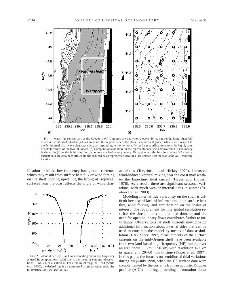
bottom intensification of the baroclinic currents occurs.The most plausible site for generating energetic internaltides in the coastal ocean is the continental shelf break,where over the distance of several kilometers bathym-etry changes from supercritical (on the continentalslope) to subcritical (on the shelf ) (Figs. 1, 2).

The Oregon coastal shelf is relatively narrow (30–50km wide) such that the internal tide propagating onshoreremains energetic up to the coast, enhancing spatial andtemporal variability in currents, mixing, and biologicalproductivity. The total M2 tidal current in this regionmay reach 15 cm s21 or more, while maximum baro-tropic (depth-averaged) currents are typically about 5cm s21 or less (Hayes and Halpern 1976; Torgrimsonand Hickey 1979; Erofeeva et al. 2003). In coastal wa-ters, internal tides show spatial variability on the scaleof several kilometers and temporal variability on thescale of days. The first-mode internal M2 horizontallength scale, estimated as 2NH/v, is 14 km in water ofdepth H 5 100 m, given a typical value of N 5 0.01s21. Topographic variation may introduce additionallength scales. One reason for high temporal variabilitymay be the spring–neap cycle (Petruncio et al. 1998).Other causes of variation may be changes in the strat-

1734 VOLUME 33J O U R N A L O F P H Y S I C A L O C E A N O G R A P H Y

FIG. 1. Maps: (a) central part of the Oregon shelf. Contours are bathymetry every 50 m, but depths larger than 750m are not contoured; shaded (white) areas are the regions where the slope is subcritical (supercritical) with respect tothe M2 internal tidal wave characteristics, corresponding to the horizontally uniform stratification shown in Fig. 2; starsdenote locations of the two HF radars. (b) Computational domain for the representer analysis and inversion [its boundaryis shown in (a) as the bold gray line]; contours are bathymetry, every 20 m; dots are the locations where HF surfacecurrent data are obtained; circles are the reduced basis representer locations (see section 3c); the star is the ADP mooringlocation.

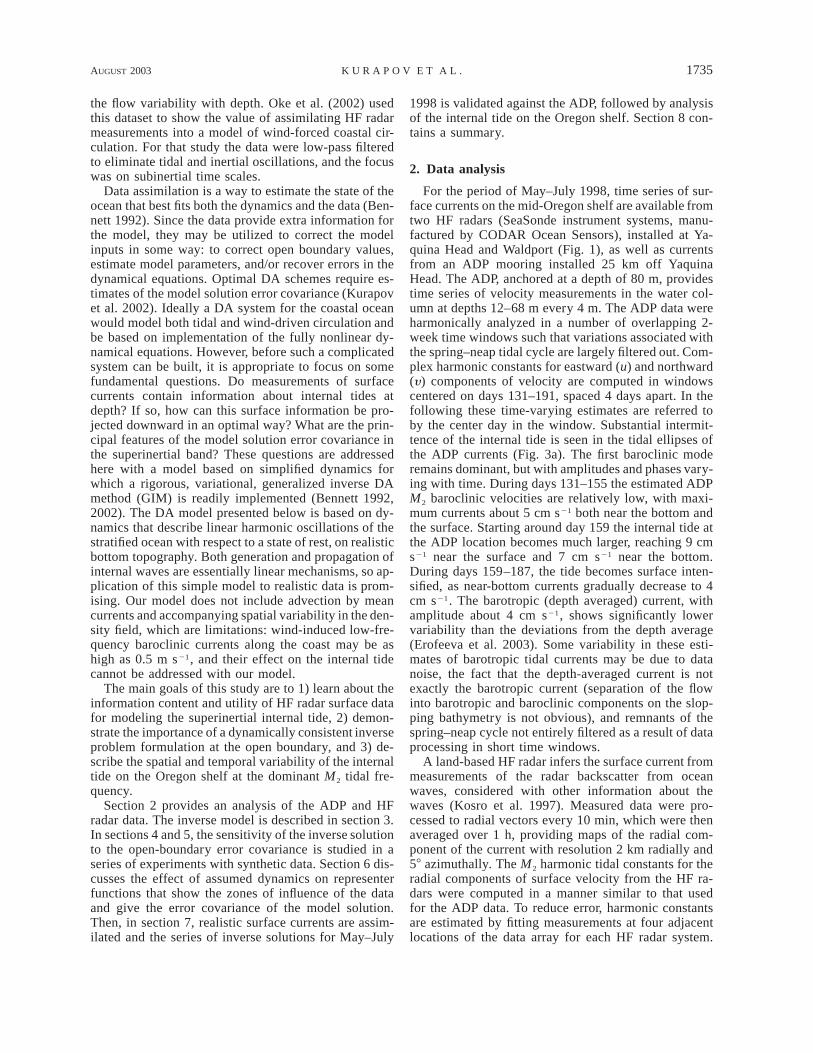
FIG. 2. Potential density and corresponding buoyancy frequencyrN used in computations: solid line is the mean of summer observa-tions, 1961–71, at a station 46 km offshore of Yaquina Head (Smithet al. 2000); the dashed line is a variant used to test solution sensitivityto stratification (see section 7a).

ification or in the low-frequency background currents,which may result from surface heat flux or wind forcingon the shelf. During upwelling the lifting of isopycnalsurfaces near the coast affects the angle of wave char-

acteristics (Torgrimson and Hickey 1979). Intensivewind-induced vertical mixing near the coast may weak-en the baroclinic tidal current (Hayes and Halpern1976). As a result, there are significant seasonal vari-ations, with much weaker internal tides in winter (Er-ofeeva et al. 2003).

Modeling internal tide variability on the shelf is dif-ficult because of lack of information about surface heatflux, wind forcing, and stratification on the scales ofinterest. The requirement for fine spatial resolution re-stricts the size of the computational domain, and theneed for open boundary flows contributes further to un-certainty. Observations of shelf currents may provideadditional information about internal tides that can beused to constrain the model by means of data assimi-lation (DA). Since 1997, measurements of the surfacecurrents on the mid-Oregon shelf have been availablefrom two land-based high-frequency (HF) radars, overan area about 50 km 3 50 km, with resolution 1–2 kmin space, and 20–60 min in time (Kosro et al. 1997).In this paper, the focus is on semidiurnal tidal variationsduring May–July 1998, when the HF surface data werecomplemented by the currents from an acoustic Dopplerprofiler (ADP) mooring, providing information about


the flow variability with depth. Oke et al. (2002) usedthis dataset to show the value of assimilating HF radarmeasurements into a model of wind-forced coastal cir-culation. For that study the data were low-pass filteredto eliminate tidal and inertial oscillations, and the focuswas on subinertial time scales.

Data assimilation is a way to estimate the state of theocean that best fits both the dynamics and the data (Ben-nett 1992). Since the data provide extra information forthe model, they may be utilized to correct the modelinputs in some way: to correct open boundary values,estimate model parameters, and/or recover errors in thedynamical equations. Optimal DA schemes require es-timates of the model solution error covariance (Kurapovet al. 2002). Ideally a DA system for the coastal oceanwould model both tidal and wind-driven circulation andbe based on implementation of the fully nonlinear dy-namical equations. However, before such a complicatedsystem can be built, it is appropriate to focus on somefundamental questions. Do measurements of surfacecurrents contain information about internal tides atdepth? If so, how can this surface information be pro-jected downward in an optimal way? What are the prin-cipal features of the model solution error covariance inthe superinertial band? These questions are addressedhere with a model based on simplified dynamics forwhich a rigorous, variational, generalized inverse DAmethod (GIM) is readily implemented (Bennett 1992,2002). The DA model presented below is based on dy-namics that describe linear harmonic oscillations of thestratified ocean with respect to a state of rest, on realisticbottom topography. Both generation and propagation ofinternal waves are essentially linear mechanisms, so ap-plication of this simple model to realistic data is prom-ising. Our model does not include advection by meancurrents and accompanying spatial variability in the den-sity field, which are limitations: wind-induced low-fre-quency baroclinic currents along the coast may be ashigh as 0.5 m s21, and their effect on the internal tidecannot be addressed with our model.

The main goals of this study are to 1) learn about theinformation content and utility of HF radar surface datafor modeling the superinertial internal tide, 2) demon-strate the importance of a dynamically consistent inverseproblem formulation at the open boundary, and 3) de-scribe the spatial and temporal variability of the internaltide on the Oregon shelf at the dominant M2 tidal fre-quency.

Section 2 provides an analysis of the ADP and HFradar data. The inverse model is described in section 3.In sections 4 and 5, the sensitivity of the inverse solutionto the open-boundary error covariance is studied in aseries of experiments with synthetic data. Section 6 dis-cusses the effect of assumed dynamics on representerfunctions that show the zones of influence of the dataand give the error covariance of the model solution.Then, in section 7, realistic surface currents are assim-ilated and the series of inverse solutions for May–July

1998 is validated against the ADP, followed by analysisof the internal tide on the Oregon shelf. Section 8 con-tains a summary.

2. Data analysis

For the period of May–July 1998, time series of sur-face currents on the mid-Oregon shelf are available fromtwo HF radars (SeaSonde instrument systems, manu-factured by CODAR Ocean Sensors), installed at Ya-quina Head and Waldport (Fig. 1), as well as currentsfrom an ADP mooring installed 25 km off YaquinaHead. The ADP, anchored at a depth of 80 m, providestime series of velocity measurements in the water col-umn at depths 12–68 m every 4 m. The ADP data wereharmonically analyzed in a number of overlapping 2-week time windows such that variations associated withthe spring–neap tidal cycle are largely filtered out. Com-plex harmonic constants for eastward (u) and northward(y) components of velocity are computed in windowscentered on days 131–191, spaced 4 days apart. In thefollowing these time-varying estimates are referred toby the center day in the window. Substantial intermit-tence of the internal tide is seen in the tidal ellipses ofthe ADP currents (Fig. 3a). The first baroclinic moderemains dominant, but with amplitudes and phases vary-ing with time. During days 131–155 the estimated ADPM2 baroclinic velocities are relatively low, with maxi-mum currents about 5 cm s21 both near the bottom andthe surface. Starting around day 159 the internal tide atthe ADP location becomes much larger, reaching 9 cms21 near the surface and 7 cm s21 near the bottom.During days 159–187, the tide becomes surface inten-sified, as near-bottom currents gradually decrease to 4cm s21. The barotropic (depth averaged) current, withamplitude about 4 cm s21, shows significantly lowervariability than the deviations from the depth average(Erofeeva et al. 2003). Some variability in these esti-mates of barotropic tidal currents may be due to datanoise, the fact that the depth-averaged current is notexactly the barotropic current (separation of the flowinto barotropic and baroclinic components on the slop-ping bathymetry is not obvious), and remnants of thespring–neap cycle not entirely filtered as a result of dataprocessing in short time windows.

A land-based HF radar infers the surface current frommeasurements of the radar backscatter from oceanwaves, considered with other information about thewaves (Kosro et al. 1997). Measured data were pro-cessed to radial vectors every 10 min, which were thenaveraged over 1 h, providing maps of the radial com-ponent of the current with resolution 2 km radially and58 azimuthally. The M2 harmonic tidal constants for theradial components of surface velocity from the HF ra-dars were computed in a manner similar to that usedfor the ADP data. To reduce error, harmonic constantsare estimated by fitting measurements at four adjacentlocations of the data array for each HF radar system.


FIG. 3. Horizontal M2 tidal current ellipses at the ADP data locations, decomposed into the depth average (shownabove the zero depth) and deviations over the water column: (a) harmonically analyzed ADP data, (b) prior solution,and (c) inverse solution obtained by assimilating HF radar radials west of longitude 235.88. Here and in Figs. 10 and13 the filled ellipses correspond to CW vector rotation; the line from the ellipse center shows the velocity direction atzero phase. In the plot, northward velocity is directed up, and eastward velocity to the right.

FIG. 4. Low-pass filtered wind stress, from wind measurements atNewport, Oregon (note that wind stress is shown here only for ref-erence, no wind forcing is applied to the model).

Only harmonic constants with estimated mean leastsquare (MLS) error , 5 cm s21 are assimilated. In thedomain shown in Fig. 1b, the mean and median of MLSerrors vary insignificantly with time, remaining close to2 cm s21.

During the study period the winds are mostly up-welling favorable (Fig. 4). This is expected to causevertical mixing in a surface boundary layer and liftingof isopycnal surfaces closer to the coast. However, welack specific empirical information about the densitystructure for this period. In the computations of the in-ternal tide the ambient potential density (z) is assumedrto be horizontally uniform and temporally constant (Fig.2). This approximation may be a serious source of error


in our model, especially later in the study period sinceduring upwelling the pycnocline structure is graduallybuilt up, and during short relaxation events (no wind)the pycnocline does not return to horizontal. However,we adopt this approximation since the inverse model isrun in a small domain, where the misspecified openboundary baroclinic flow is hypothesized to be a largersource of error.

3. Inverse model

a. Model equations

The model describes linear harmonic oscillations ofthe stratified ocean with respect to the state of rest.Boussinesq and hydrostatic approximations are made.State variables vary with time as exp(ivt). The modelis written in horizontal Cartesian coordinates with x tothe east, y to the north. Linearized surface boundaryconditions are applied at the mean sea surface level (z5 0). The vertical coordinate is stretched into s 5 z/H(x, y), and so the model equations are (cf. Blumbergand Mellor 1987; Mellor 1998):

ivHu 1 f 3 Hu 1 gH=h

02gH =H ]r1 =r 2 s9 ds9E 1 2r H ]s9o s

] K ]uM2 5 0, (2)1 2]s H ]s

]w1 = · (Hu) 5 0, (3)

]s

]ivHr 1 (rw) 1 = · (rHu) 5 0. (4)

]s

In (2)–(4), all the dynamic variables represent complexamplitudes: u(x, y, s) 5 {u, y} is the horizontal velocityvector, h(x, y) is the surface elevation, r(x, y, s) is thepotential density perturbation about a horizontally uni-form mean state (z) 5 (x, y, s), and w(x, y, s) is ther rvelocity component normal to the s-surfaces (w 5 wcart

2 su · =H, where wcart is the Cartesian vertical velocitycomponent in the unstretched coordinates); the param-eters to be specified are gravity g, the Coriolis parameterf 5 const, the vertical eddy viscosity KM(x, y, s), ba-thymetry H(x, y) and the reference density ro 5 const;= and = · are the ‘‘horizontal’’ gradient and divergenceoperators on a s surface.

Vertical dissipation in (2) is the only sink of energyin the model and it is a very simple and admittedlycrude parameterization of turbulence associated withbackground flows. A horizontal diffusion term is notincluded in (2), partly for a technical reason, to allowthe solution of the momentum equations in terms ofvelocity locally for each vertical column (see appendixA). In fact, for coastal applications, horizontal dissi-

pation is a minor contributor to the momentum balance.Since we do not solve the problem by time stepping,horizontal dissipation is not needed for computationalstability. Vertical diffusion of r is not included in (4).This simplifies the energy balance and is consistent withthe assumption that vertical diffusion does not have ef-fect on the background (z).r

Surface and bottom boundary conditions, at s 5 0and s 5 21, are

]u5 0 at s 5 0, (5)

]s

w 5 ivh at s 5 0, (6)

w 5 0 at s 5 21, (7)

K ]uM 5 ru at s 5 21, (8)H ]s

where r(x, y) is the bottom drag coefficient.A depth-integrated continuity equation is obtained

with use of (3), (6), and (7):

0

ivh 1 = · Hu ds 5 0. (9)E21

At the side boundaries G the normal current u · n isspecified pointwise:

0 at the coastu · n| 5 (10)G 5u at the open boundary.OB

Since horizontal advective terms are dropped from theequations, the problem with boundary condition (10) isformally well posed, in the sense that it has a uniquesolution which is stable to changes in inputs (Oliger andSundstrom 1978; see also Bennett 1992, chapter 9). Theopen boundary condition (10) is in general reflective.However, we are going to treat the boundary conditionas imperfect and correct open boundary baroclinic flux-es. This can be done in such a way to improve waveradiation out of the domain.

Once the dynamics are defined, the GIM requiresspecification of a cost functional that is a weighted sumof terms, each penalizing errors in the inputs such asthe model equations, boundary conditions, or data. Thiscan be minimized in an efficient way if the problem isseparated into a series of so called adjoint and forwardproblems (see Bennett 1992, 2002; Egbert et al. 1994).Technically, there are two approaches to formulating thegeneralized inverse problem that eventually differ inhow the adjoint model is built (Sirkes and Tziperman1997). In the first approach, the cost functional penalizesthe errors in the continuous equations and boundaryconditions (2)–(10), and the finite-difference imple-mentation is formulated independently for the forwardand adjoint problems derived in continuous form. In thesecond approach, to be taken here, the cost functionalpenalizes errors in the discretized dynamical equations


and boundary conditions. The advantage of this ap-proach in our case is that the discrete adjoint solver willbe obtained as a matrix transpose of the forward solver,simplifying derivation, as well as computer coding, forrepresenter calculation.

b. Model discretization

The equations and boundary conditions are discreti-zed on a staggered Arakawa C grid, with details as inBlumberg and Mellor (1987), and Mellor (1998). Then,state variables at the points of the discrete grid are com-bined into vectors of unknowns u, w, h, and r, cor-responding to continuous Hu, w, h, and r. Discretizedmodel equations can be written in matrix notation as

Vu 1 Gh 1 Pr 5 f , (11)u

ivh 1 D u 5 f , (12)a a

Ww 1 Du 5 f , (13)w

Br 1 Z w 1 D u 5 f , (14)r r r

where (11) represents horizontal momentum equations(2) combined with boundary conditions (5), (8), and(10); (12) represents the depth-integrated continuityequation (9); (13) is for the continuity equation (3) com-bined with the bottom boundary condition (7); and (14)is the discrete representation of the equation for thepotential density (4). In (11)–(14), V, G, and so on, arethe coefficient matrices resulting from discretization,and fu, fa, etc., are forcing vectors. If the state variablesand the forcing vectors are combined into

u f u

w f wn 5 and f 5 , (15) h fa r f r

then Eqs. (11)–(14) can be formally written together as

Sn 5 f, (16)

where S is the model operator (matrix). In general, theforcing vector f can be written as f 5 f0 1 e, where f0

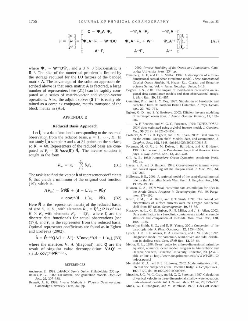
is the vector of boundary values and e represents errorsin the discretized equations and boundary conditions.Although in our study most of the elements of e arealways zero, we retain the general weak constraint for-mulation for future convenience (see section 3c). Anefficient approach that we utilize to solve (16) for anarbitrary f is based on the direct factorization of themodel operator (Egbert and Erofeeva 2002), as de-scribed in appendix A.

c. Cost function and inverse solution

Data to be assimilated can be written in the generalform

d 5 l9n 1 e ,k k dk (17)

where the vector lk is the discrete data functional, theprime denotes the complex conjugate matrix transpose,dk is the kth scalar observation value, edk is the dataerror, and k 5 1, . . . , K. All the data can be combinedin one matrix equation:

d 5 L9n 1 e .d (18)

The inverse solution minimizes the cost function:21J(n) 5 (Sn 2 f )9 cov (Sn 2 f )0 0

211 (d 2 L9n)9 cov (d 2 L9n), (19)d

where cov and covd are the Hermitian non-negativedefinite covariance matrices of errors in the model equa-tions and the data, respectively. These have to be spec-ified prior to inversion. In the statistical interpretationof the GIM, the errors are treated as random vectors,so cov 5 êe9& and covd 5 êd &, where angle bracketse9ddenote ensemble average. It is also assumed that dy-namics and measurements are unbiased: ê& 5 0, andêd& 5 0.

In our case, the first term in (19) incorporates pen-alties on both the dynamical equations and boundaryconditions. If the errors in the dynamical equations andboundary conditions are assumed to be uncorrelated,this term can be written as the sum of penalties on theerrors in these two sources. Note that, in general, dy-namical and open boundary condition errors may becorrelated (Bogden 2001). The inverse solution can beexpressed as

K

n 5 n 1 b r , (20)Oinv 0 k kk51

where n0 5 S21f0 is the prior solution satisfying error-free equations (11)–(14),

21 21r 5 S cov(S9) lk k (21)

are representer vectors, coefficients bk in (20) are ele-ments of vector b, of size K:

21b 5 (R 1 cov ) (d 2 L9n ),d 0 (22)

and R is the representer matrix with elements Rkj 5 r j.l9kThe representer shows the zone of influence of each

observation in the model domain. It can be partitionedinto fields each providing correction to prior u, y, w, h,and r. In (21), (S9)21lk is the adjoint representer solution,which gives the sensitivity of the kth observation tochanges in forcing and boundary conditions. It is mul-tiplied by the covariance, which usually has a smoothingeffect (see Egbert et al. 1994). Last, the ‘‘forward’’ prob-lem (21) is solved. Our solution method for (16) allowsrapid computation of a large number of representers (seeappendix A). In our formulation, all the equations andboundary conditions are written as weak constraints.Strong constraint cases are recovered simply by settingthe appropriate parts of cov to 0.

In the statistical interpretation of the GIM, repre-senters give the prior error covariance for the model


solution. Specifically, if e0 5 n0 2 ntrue is the error inthe prior solution, then

r 5 ^e e9&l .k 0 0 k (23)

In this interpretation, (Rjj)1/2 is the expected prior errorof the sampled quantity. Since the representer does notdepend on the actual observed value, but only on theform of lk and assumed cov [see (21)], the expectedvariability of the model solution can in principle beassessed for any variable at any point. This propertywill be used to compute the open boundary covarianceby nesting (section 4).

In the area shown in Fig. 1b harmonic constants forthe radial components of surface velocities from the HFradars are available at over 900 locations. Computationof the full set of representers would be costly. Conse-quently, a reduced basis approach is taken (Egbert andErofeeva 2002), as detailed in appendix B. A set of 68representers, chosen as a reduced basis for model cor-rection, is computed for data functionals lk correspond-ing to u and y at a fixed set of 34 surface locations (seeFig. 1b). The sum in (20) is replaced by a linear com-bination of the representers of the reduced basis [see(B1)]. A vector b of 68 representer coefficients is soughtto minimize the original cost function (19), that is, withall the data in the second penalty term. Note that noactual u and y data are measured at the reduced basislocations and the radial components from the two HFradars do not have to be reprocessed to obtain u and ycomponents. The inverse solution inv obtained with thenreduced representer basis should be a close approxi-mation of ninv, obtained with the full basis, providedrepresenters for all the radial data can be approximatedwell as a linear combination of representers from thereduced basis set. With this approach, the same rela-tively small representer basis is used to find the solutionin every time window, while the number and locationof harmonically analyzed HF radar data meeting ouraccuracy threshold (see section 2) vary with time.

d. Computational setup

Most computations have been performed for the 38km 3 56 km area shown in Fig. 1b that has a maximumdepth of 250 m and includes Stonewall Bank, a moderatebathymetric rise. In this area, the data from both HFradars, at Yaquina Head and Waldport, provide infor-mation about two components of surface currents (Kos-ro et al. 1997). The computational grid has 1-km res-olution in the horizontal and 21 s levels in the vertical.Some computations described in sections 4 and 5 havealso been performed for larger domains, at 2- and 3-kmresolution.

Some dissipation is needed for numerical stability, tosmear sharp gradients across wave beams resulting fromthe singular forcing of the adjoint solution [see (21)].Vertical eddy viscosity is taken to be horizontally uniformand varying with depth as KM 5 1022 exp[2(z/10)4] 1

1024 (m2 s21). Thus KM approaches 1022 m2 s21 in theupper 10 m (Wijesekera et al. 2003) and 1024 m2 s21 indeeper water [a minimum value based on the parame-terization of Pacanowski and Philander (1981)]. Increas-ing KM to a constant value of 1022 m2 s21 everywherein the computational domain makes representer functionssmoother and has only minor effects on the inverse so-lution. The linear bottom friction coefficient is a constantr 5 2.5 3 1024 m s21. Unless otherwise specified, themean of summer observations, 1961–71, at a station 46km offshore of Yaquina Head (Smith et al. 2000) defines

(z) (the solid line in Fig. 2).rThe prior model is forced at the open boundary by

barotropic (depth averaged) currents, taken from acoastal-scale tidal inverse model in which TOPEX/Po-seidon altimetry data are assimilated into the shallow-water equations (Egbert and Erofeeva 2002). The sameprior solution is used in each time window. The priorsolution provides an accurate estimate of the barotropicsemidiurnal flow in the area (Erofeeva et al. 2003).However, deviations from the depth average are muchsmaller in the prior solution than in the ADP data (cf.Figs. 3b, and 3a), suggesting that most baroclinic signalpropagates into the study area from outside. It is thusessential to estimate baroclinic fluxes at the open bound-ary (OB). This is done by means of DA.

To obtain an inverse solution, cov and covd shouldbe specified. A great deal of uncertainty still exists abouterror statistics of HF radar data. Contributing factorsinclude instrumental and processing errors, environ-mental conditions that affect signal scattering, and rep-resentation of the measurement in the dynamical model(i.e., the choice of lk). In the absence of detailed infor-mation about all these factors, in this study we assumethe simplest diagonal covariance matrix for data errors,covd 5 I, where sd 5 0.02 m s21 is based on typical2s d

MLS errors of the harmonic constants, and I is the iden-tity matrix.

4. Error covariance for the OB condition

Although errors in the linearized equations are surelynot zero, we hypothesize that the major source of so-lution error in our small domain is the open boundarycondition (10) and take this to be the only weak con-straint. Thus, the rhs of Eqs. (11)–(14) will all be 0except in the rows corresponding to open boundarynodes, where fu is equal to the specified barotropic cur-rent plus the error that is estimated through DA. Ac-cordingly, in the matrix cov [see (21)] the only nonzeroentries are the elements corresponding to the spatialcovariance of OB fluxes: C(xj, sj; xk, sk) 5 ^q(xj,sj)q9(xk, sk)&, where (x, s) 5 (x, y, s) are positions onthe OB, and q represents u at the western boundary andy at the northern or southern boundary of our rectangulardomain.

In an oceanographic context, the input error covari-ances are known only approximately, at best. In practice,


the choice of covariance is guided by both the need tosatisfy (at least approximately) a number of physicalconstraints and by ease of implementation. In our case,physical constraints with which the open boundary co-variance must be consistent include the following: (i)at the OB, correction is provided only to deviations fromthe depth-average current (recall that deviations fromthe depth-average at the OB are 0 in the prior solution,while depth-averaged currents are believed to be rea-sonably accurate); (ii) u at the west, and y at the northand south boundary segments are correlated in a wayto avoid nonphysical solution behavior in the cornersof the computational domain; (iii) the expected priorerror of the velocity at the OB is of the order of a fewcentimeters per second (this requirement can be readilysatisfied by scaling the covariance); (iv) low verticalmodes are dominant; and (v) the covariance has a dy-namically consistent spatial structure since, for instance,propagating modes are correlated at different parts ofthe boundary in accordance with their phase speed anddirection of propagation. This list of constraints for thecovariance can be refined and completed as more ex-perience is gained in regional DA modeling, for ex-ample, via the analysis of the representers and the in-verse solution.

We tested two covariances that differ in the extent towhich criterion (v) is addressed. The Type I covarianceis constructed in an ad hoc manner guided by the prin-ciples outlined above. The hope with such an approach,which has been frequently used in the past, is that thecovariance enforces smoothing and thus regularizes theinverse problem, but details of structure do not matterso much. The Type II covariance is obtained followinga nesting approach, using the representer solution in alarger domain.

The Type I covariance is assumed to be separable as

C(x , s ; x , s ) 5 C (x , x )C (s , s ),j j k k 1 j k 2 j k (24)

where C1 and C2 are both symmetric and positive def-inite. To ensure regularity of u and y around corners(criterion ii), velocity u in a s layer is partitioned intoa nondivergent flow, described by a streamfunction c,and an irrotational flow, described by a potential f.Spatial correlations for both ^cc& and ^ff& are assumedto have a Gaussian form, with ^cf& 5 0. Then C1 isobtained in the standard way as a linear combination ofderivatives of ^cc& and ^ff&. To derive C2, the errorsin the OB boundary condition are projected onto localflat bottom rigid-lid baroclinic vertical modes associatedwith stratification N(z), and the modal amplitudes areassumed to be uncorrelated (Kurapov et al. 2002).

Our construction of the Type I covariance is alreadyquite involved, and yet some rather obvious issues (e.g.,appropriate phase velocities along the boundaries) havenot even been considered. Nesting, based on the inter-pretation of the representers as covariances [see (23)],provides a simpler and more general approach to con-struction of a physically consistent covariance for the

OB condition. The Type II covariance for u and y atthe boundary of the local grid can be obtained as a resultof the representer computation on a larger, coarser-res-olution grid. In our application, the local grid is nestedin a large-scale grid covering an area of 177 km 3 435km with 3-km resolution in the horizontal and 11 ssurfaces in the vertical (this domain is larger than thearea shown in Fig. 1a); maximum water depth is set to500 m. For the large-scale grid, the open boundary con-dition is a strong constraint, and the horizontal mo-mentum equation (2) is a weak constraint. To form ma-trix cov for the large-scale model, the covariance forthe errors in each u and y component of Eq. (2) is writtenas in (24) with xj and xk now inside the domain. HereC1 is Gaussian with a decorrelation length scale of 10km and C2 is as above, based on the local flat bottommodal decomposition. The Type II covariance is com-puted on the large-scale grid as a representer matrix forvelocity observations at the locations corresponding tothe OB nodes of the small, nested domain (observationsare for u at the west, and y at the north and south).

Figure 5 illustrates the difference in the spatial patternof the Type I and Type II covariances at the northernboundary. Distinctive features of the Type II covarianceare determined by the superinertial wave dynamics inthe stratified medium. The first baroclinic mode is pre-served, indicated by the 1808 phase difference betweenthe surface and bottom. In contrast to the strictly real-valued Type I covariance, the Type II covariance iscomplex-valued allowing for progressive phase changesalong the boundary. The fact that energy (and henceinformation) propagates along wave characteristicsmanifests itself in the pattern of phase lines oriented atan angle to the horizontal. For the assumed (z), therbottom slope near the coast is close to critical (see Fig.1a), and here energy density may be intensified near thebottom. Accordingly, the covariance amplitude, as wellas the expected prior error, is increased at this spot.

In the ‘‘hand-made’’ Type I covariance (see Fig. 5b),the first baroclinic mode is also dominant, by construc-tion. However, the other dynamically realistic featuresevident in the Type II covariance are missing.

5. Computations with synthetic data: Effect of theOB condition error covariance

When inverting HF radar surface currents (section 7),ADP velocities are available to validate the data assim-ilation results only at one location. To see better howthe choice of the covariance for the open boundary con-dition (section 4) affects the solution everywhere in thecomputational domain, tests with synthetic data havebeen performed. To generate synthetics we first computethe model solution for the larger 94 km 3 150 km areashown in Fig. 1a, forced with depth-averaged currentsfrom the shallow-water inverse model. In this area, aninternal tide with an amplitude comparable to obser-vations at the ADP site is generated over the shelf break.


FIG. 5. Error covariance of y at the location shown as the star andy9 everywhere else at the northern boundary: (a) Type II covariance(obtained by nesting), complex amplitude is indicated by shading,phase is contoured; (b) Type I covariance [real valued, 908 phase linedivides positive (at the top) and negative (near the bottom) values].

FIG. 6. Effect of the OB error covariance on the rms differencebetween the inverse and validation u for a range of weights wo inthe computations with synthetic data. Thick lines: total rms; thin lines:depth-average rms at the ADP location. Solid lines correspond to theType II covariance (obtained by nesting) and dashed lines to the TypeI covariance.

This solution is obtained with resolution 2 km 3 2 kmin the horizontal, and 11 s surfaces in the vertical, withthe maximum water depth set at 500 m. The total, depth-dependent currents obtained from the 2-km resolutionsolution are then used to force the model in the small,higher-resolution domain to generate a validation so-lution. Synthetic u and y data are sampled from thissolution at 34 surface locations, shown as circles in Fig.1b, and random noise of amplitude 0.02 m s21 is added.The inverse solution obtained with these synthetic datais compared with the validation solution by computingthe rms difference of the complex-valued three-dimen-sional velocity fields.

Since the choice of covariances in the cost function(19) is always a hypothesis, it is important to learn aboutsensitivity of the inverse solution to their specification.In reality, uncertainty exists first of all about the mag-nitude of the errors, both for the model and the data.The relative amplitude of the assumed errors in the in-

puts can be controlled by scaling the covariances in (19).Let us replace the covariance cov with cov, where21wo

wo is a scaling factor for the open boundary penaltyterm in the cost functional (we again consider a strongconstraint case, so only OB elements of cov are non-zero). The rms error of the inverse solutions, computedwith the Type I and Type II covariances, is plotted asa function of wo in Fig. 6, where the total rms error isaveraged over the whole domain. For large values ofwo the solution rms error is close to that for the priorsolution. The minimum rms error is attained for wo 51 both for Type I and Type II covariances. For lowerwo, the surface data is fit better, but the DA modelperformance deteriorates. Very low values of wo cor-respond to the case of effectively no open boundarycondition penalty term in the cost function. The problembecomes ill-conditioned; solution irregularities originatenear the open boundary and propagate inside the domain(Foreman et al. 1980; Kivman 1997). In our case, spu-rious small scale baroclinic vertical modes appear in thesolution for low wo.

For the full range of wo, the inverse solution obtainedwith the Type II covariance has a smaller total rms errorthan that obtained with the Type I covariance. Further-more, for wo , 1 the Type II solution is much lesssensitive to weight misspecification than Type I. Over-estimating the expected open boundary error amplitudeby an order of magnitude corresponds to wo 5 0.01 andfor this weight the Type I covariance yields a solutionwith rms error already worse than the prior, while theType II solution still provides improvement. For smallwo, the total rms error is larger than the depth-averagerms error at the ADP location, indicating that the so-lution quality is worse at the boundaries. This is illus-


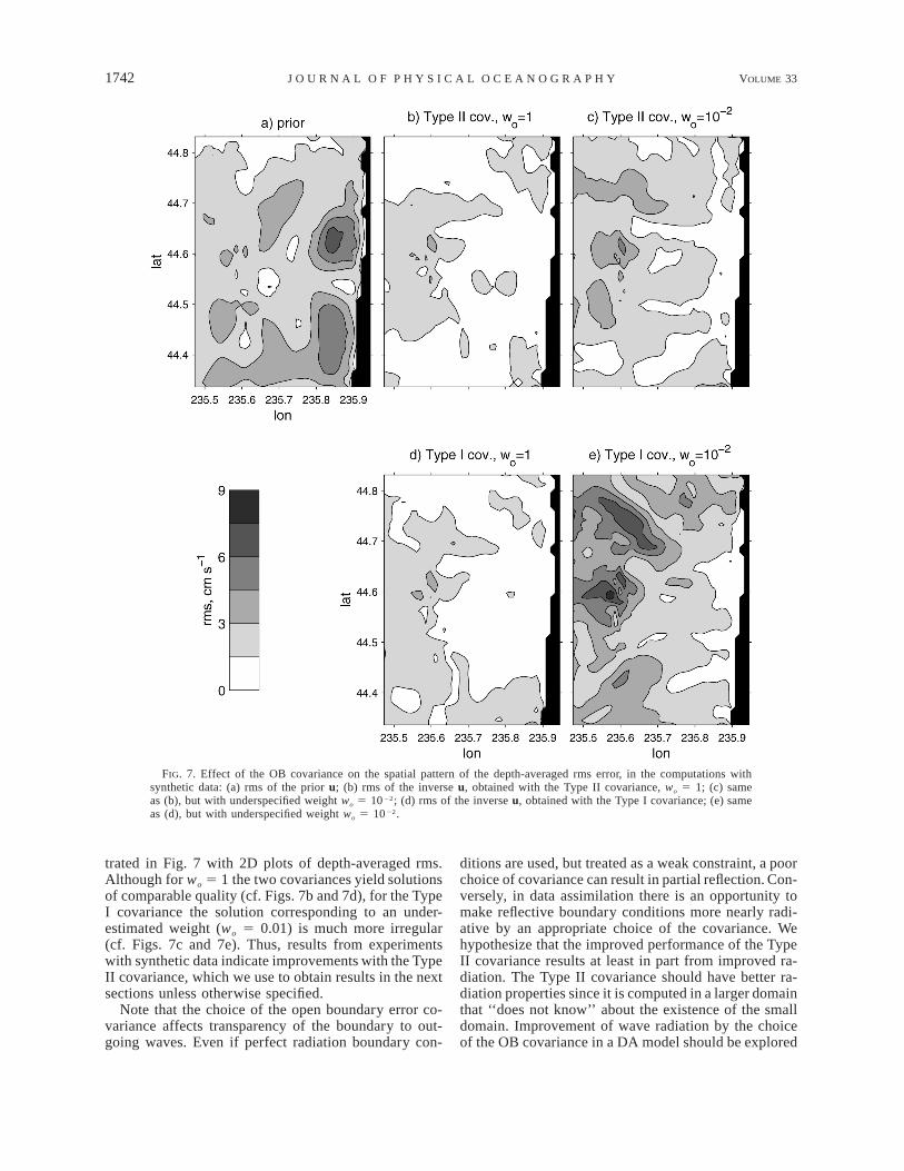
FIG. 7. Effect of the OB covariance on the spatial pattern of the depth-averaged rms error, in the computations withsynthetic data: (a) rms of the prior u; (b) rms of the inverse u, obtained with the Type II covariance, wo 5 1; (c) sameas (b), but with underspecified weight wo 5 1022; (d) rms of the inverse u, obtained with the Type I covariance; (e) sameas (d), but with underspecified weight wo 5 1022.

trated in Fig. 7 with 2D plots of depth-averaged rms.Although for wo 5 1 the two covariances yield solutionsof comparable quality (cf. Figs. 7b and 7d), for the TypeI covariance the solution corresponding to an under-estimated weight (wo 5 0.01) is much more irregular(cf. Figs. 7c and 7e). Thus, results from experimentswith synthetic data indicate improvements with the TypeII covariance, which we use to obtain results in the nextsections unless otherwise specified.

Note that the choice of the open boundary error co-variance affects transparency of the boundary to out-going waves. Even if perfect radiation boundary con-

ditions are used, but treated as a weak constraint, a poorchoice of covariance can result in partial reflection. Con-versely, in data assimilation there is an opportunity tomake reflective boundary conditions more nearly radi-ative by an appropriate choice of the covariance. Wehypothesize that the improved performance of the TypeII covariance results at least in part from improved ra-diation. The Type II covariance should have better ra-diation properties since it is computed in a larger domainthat ‘‘does not know’’ about the existence of the smalldomain. Improvement of wave radiation by the choiceof the OB covariance in a DA model should be explored


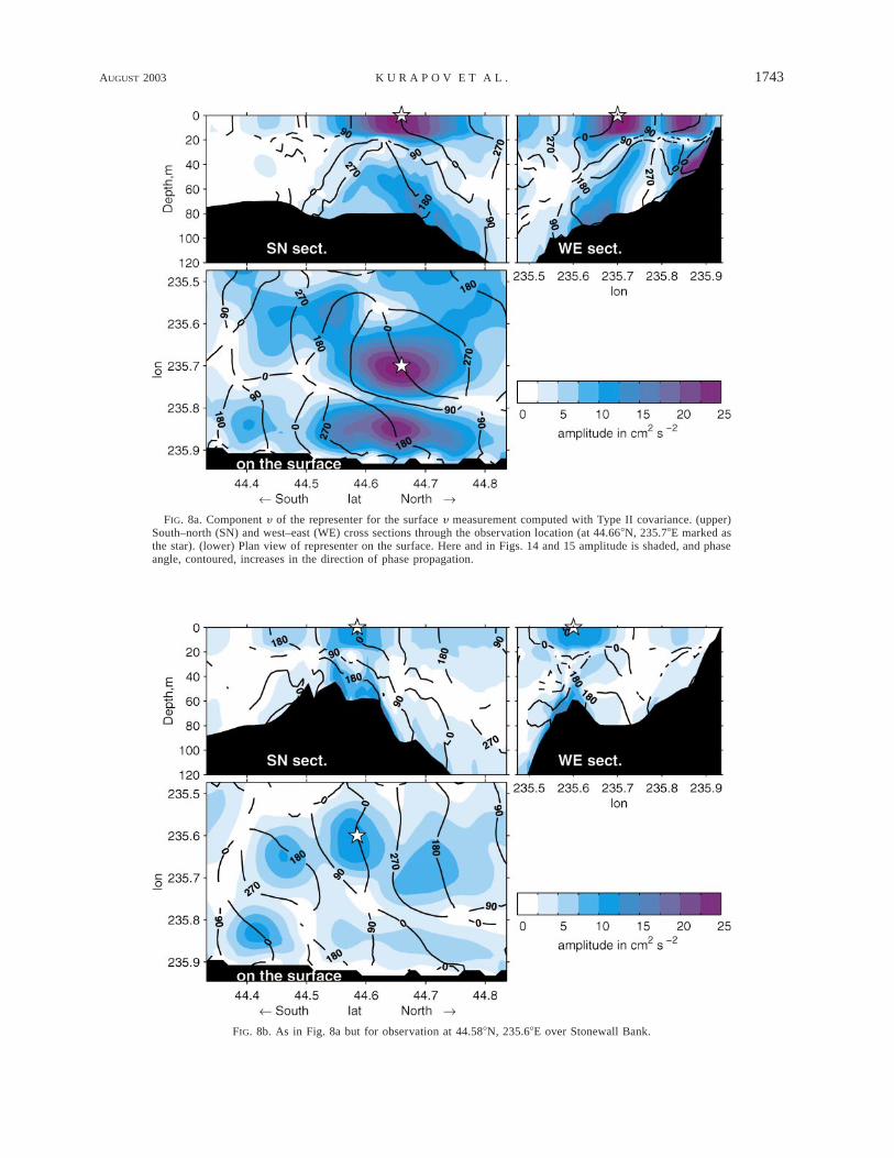
FIG. 8a. Component y of the representer for the surface y measurement computed with Type II covariance. (upper)South–north (SN) and west–east (WE) cross sections through the observation location (at 44.668N, 235.78E marked asthe star). (lower) Plan view of representer on the surface. Here and in Figs. 14 and 15 amplitude is shaded, and phaseangle, contoured, increases in the direction of phase propagation.

FIG. 8b. As in Fig. 8a but for observation at 44.588N, 235.68E over Stonewall Bank.


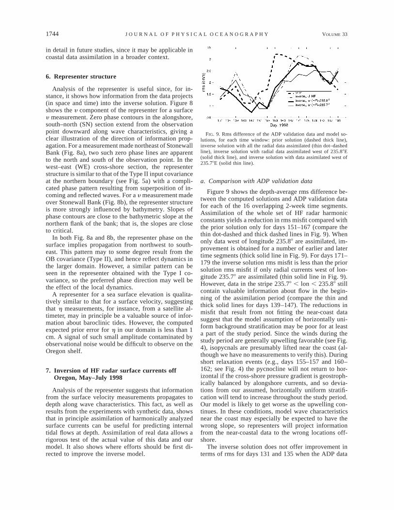
FIG. 9. Rms difference of the ADP validation data and model so-lutions, for each time window: prior solution (dashed thick line),inverse solution with all the radial data assimilated (thin dot–dashedline), inverse solution with radial data assimilated west of 235.88E(solid thick line), and inverse solution with data assimilated west of235.78E (solid thin line).

in detail in future studies, since it may be applicable incoastal data assimilation in a broader context.

6. Representer structure

Analysis of the representer is useful since, for in-stance, it shows how information from the data projects(in space and time) into the inverse solution. Figure 8shows the y component of the representer for a surfacey measurement. Zero phase contours in the alongshore,south–north (SN) section extend from the observationpoint downward along wave characteristics, giving aclear illustration of the direction of information prop-agation. For a measurement made northeast of StonewallBank (Fig. 8a), two such zero phase lines are apparentto the north and south of the observation point. In thewest–east (WE) cross-shore section, the representerstructure is similar to that of the Type II input covarianceat the northern boundary (see Fig. 5a) with a compli-cated phase pattern resulting from superposition of in-coming and reflected waves. For a y measurement madeover Stonewall Bank (Fig. 8b), the representer structureis more strongly influenced by bathymetry. Slopes ofphase contours are close to the bathymetric slope at thenorthern flank of the bank; that is, the slopes are closeto critical.

In both Fig. 8a and 8b, the representer phase on thesurface implies propagation from northwest to south-east. This pattern may to some degree result from theOB covariance (Type II), and hence reflect dynamics inthe larger domain. However, a similar pattern can beseen in the representer obtained with the Type I co-variance, so the preferred phase direction may well bethe effect of the local dynamics.

A representer for a sea surface elevation is qualita-tively similar to that for a surface velocity, suggestingthat h measurements, for instance, from a satellite al-timeter, may in principle be a valuable source of infor-mation about baroclinic tides. However, the computedexpected prior error for h in our domain is less than 1cm. A signal of such small amplitude contaminated byobservational noise would be difficult to observe on theOregon shelf.

7. Inversion of HF radar surface currents offOregon, May–July 1998

Analysis of the representer suggests that informationfrom the surface velocity measurements propagates todepth along wave characteristics. This fact, as well asresults from the experiments with synthetic data, showsthat in principle assimilation of harmonically analyzedsurface currents can be useful for predicting internaltidal flows at depth. Assimilation of real data allows arigorous test of the actual value of this data and ourmodel. It also shows where efforts should be first di-rected to improve the inverse model.

a. Comparison with ADP validation data

Figure 9 shows the depth-average rms difference be-tween the computed solutions and ADP validation datafor each of the 16 overlapping 2-week time segments.Assimilation of the whole set of HF radar harmonicconstants yields a reduction in rms misfit compared withthe prior solution only for days 151–167 (compare thethin dot-dashed and thick dashed lines in Fig. 9). Whenonly data west of longitude 235.88 are assimilated, im-provement is obtained for a number of earlier and latertime segments (thick solid line in Fig. 9). For days 171–179 the inverse solution rms misfit is less than the priorsolution rms misfit if only radial currents west of lon-gitude 235.78 are assimilated (thin solid line in Fig. 9).However, data in the stripe 235.78 , lon , 235.88 stillcontain valuable information about flow in the begin-ning of the assimilation period (compare the thin andthick solid lines for days 139–147). The reductions inmisfit that result from not fitting the near-coast datasuggest that the model assumption of horizontally uni-form background stratification may be poor for at leasta part of the study period. Since the winds during thestudy period are generally upwelling favorable (see Fig.4), isopycnals are presumably lifted near the coast (al-though we have no measurements to verify this). Duringshort relaxation events (e.g., days 155–157 and 160–162; see Fig. 4) the pycnocline will not return to hor-izontal if the cross-shore pressure gradient is geostroph-ically balanced by alongshore currents, and so devia-tions from our assumed, horizontally uniform stratifi-cation will tend to increase throughout the study period.Our model is likely to get worse as the upwelling con-tinues. In these conditions, model wave characteristicsnear the coast may especially be expected to have thewrong slope, so representers will project informationfrom the near-coastal data to the wrong locations off-shore.

The inverse solution does not offer improvement interms of rms for days 131 and 135 when the ADP data


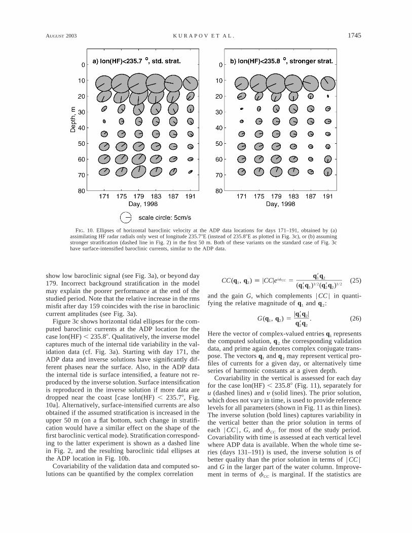
FIG. 10. Ellipses of horizontal baroclinic velocity at the ADP data locations for days 171–191, obtained by (a)assimilating HF radar radials only west of longitude 235.78E (instead of 235.88E as plotted in Fig. 3c), or (b) assumingstronger stratification (dashed line in Fig. 2) in the first 50 m. Both of these variants on the standard case of Fig. 3chave surface-intensified baroclinic currents, similar to the ADP data.

show low baroclinic signal (see Fig. 3a), or beyond day179. Incorrect background stratification in the modelmay explain the poorer performance at the end of thestudied period. Note that the relative increase in the rmsmisfit after day 159 coincides with the rise in barocliniccurrent amplitudes (see Fig. 3a).

Figure 3c shows horizontal tidal ellipses for the com-puted baroclinic currents at the ADP location for thecase lon(HF) , 235.88. Qualitatively, the inverse modelcaptures much of the internal tide variability in the val-idation data (cf. Fig. 3a). Starting with day 171, theADP data and inverse solutions have significantly dif-ferent phases near the surface. Also, in the ADP datathe internal tide is surface intensified, a feature not re-produced by the inverse solution. Surface intensificationis reproduced in the inverse solution if more data aredropped near the coast [case lon(HF) , 235.78, Fig.10a]. Alternatively, surface-intensified currents are alsoobtained if the assumed stratification is increased in theupper 50 m (on a flat bottom, such change in stratifi-cation would have a similar effect on the shape of thefirst baroclinic vertical mode). Stratification correspond-ing to the latter experiment is shown as a dashed linein Fig. 2, and the resulting baroclinic tidal ellipses atthe ADP location in Fig. 10b.

Covariability of the validation data and computed so-lutions can be quantified by the complex correlation

q9q1 2ifCCCC(q , q ) [ |CC|e 5 (25)1 2 1/2 1/2(q9q ) (q9q )1 1 2 2

and the gain G, which complements | CC | in quanti-fying the relative magnitude of q1 and q2:

|q9q |1 2G(q , q ) 5 . (26)1 2 q9q2 2

Here the vector of complex-valued entries q1 representsthe computed solution, q2 the corresponding validationdata, and prime again denotes complex conjugate trans-pose. The vectors q1 and q2 may represent vertical pro-files of currents for a given day, or alternatively timeseries of harmonic constants at a given depth.

Covariability in the vertical is assessed for each dayfor the case lon(HF) , 235.88 (Fig. 11), separately foru (dashed lines) and y (solid lines). The prior solution,which does not vary in time, is used to provide referencelevels for all parameters (shown in Fig. 11 as thin lines).The inverse solution (bold lines) captures variability inthe vertical better than the prior solution in terms ofeach | CC | , G, and fCC for most of the study period.Covariability with time is assessed at each vertical levelwhere ADP data is available. When the whole time se-ries (days 131–191) is used, the inverse solution is ofbetter quality than the prior solution in terms of | CC |and G in the larger part of the water column. Improve-ment in terms of fCC is marginal. If the statistics are


FIG. 11. Functions showing ADP-prior and ADP-inverse solutioncovariability in the vertical, for each day: amplitude | CC | and phasefCC of complex correlation, and gain G (26), where q2 represents theADP measurements; lon(HF) , 235.88E.

FIG. 12. Functions showing ADP-prior and ADP-inverse solution covariability with time, ateach depth [lon(HF) , 235.88E]: statistics for days 139–167, for which the solution rms error isimproved. Legend as in Fig. 11. Values corresponding to rms amplitudes of the ADP fluctuationcurrents , 1 cm s21 are not shown.

computed only for days 139–167 for which the solutionrms error is improved, the inverse solution is of betterquality than the prior solution in terms of all the threecriteria (Fig. 12). Note that at middepths, where themagnitude of the baroclinic currents is low, estimatesof CC and G lose meaning. The fact that all the criteriaare improved below 40 m provides a clear demonstrationof the value of surface currents from HF radars in con-straining subsurface tidal flows.

Our results suggest that the assumption of horizon-tally uniform background stratification is a significantdeficiency in our model. To the extent that this is true,our initial hypothesis that the only significant source oferror is in the open boundary forcing is questionable.The hypothesis about the errors can be tested formally(Bennett 2002, his section 2.3.3). Under the assumptionthat the errors are Gaussian with zero mean and co-variance cov and covd, twice the cost function 2J(ninv)is itself a random variable having a x2 distribution with2K degrees of freedom (a factor of 2 appears since thedata are complex valued); recall K is the number ofassimilated data (K ø 540 in the case lon(HF) , 235.88).In particular, the mean value of 2J(ninv) should be 2Kand the variance 4K. Note that the reduced basis estimateJ( inv) (B2) is larger then the full basis estimate J(ninv),nalthough these values should be close since inv ø ninv.nFor our series of inverse solutions J( inv)/K is in thenrange of 2–12 implying that hypothesis about errorsshould be rejected. The data term in J( inv) accounts fornabout 95% of the total cost function value, so changingcovd should have a stronger effect on J( inv) than cov.nIn this respect, better knowledge of the error model forthe data would be desirable.

By itself the x2 criterion does not say where the de-ficiency in our hypothesis is; e.g., either one or both ofcov and covd could be misspecified. Increasing our es-timate of the data error standard deviations from 2 to 3cm s21 decreases J( inv)/K to a value near 1 over muchnof the first half of the study. Such an increase in dataerror is quite plausible. However, in the second half ofthe study, when J( inv)/K . 6, unreasonably large in-ncreases in the data error would be required to bring thetest statistics down to acceptable levels, implying thatsome modifications to cov are required at least for thistime period. Increasing the expected magnitude of errors


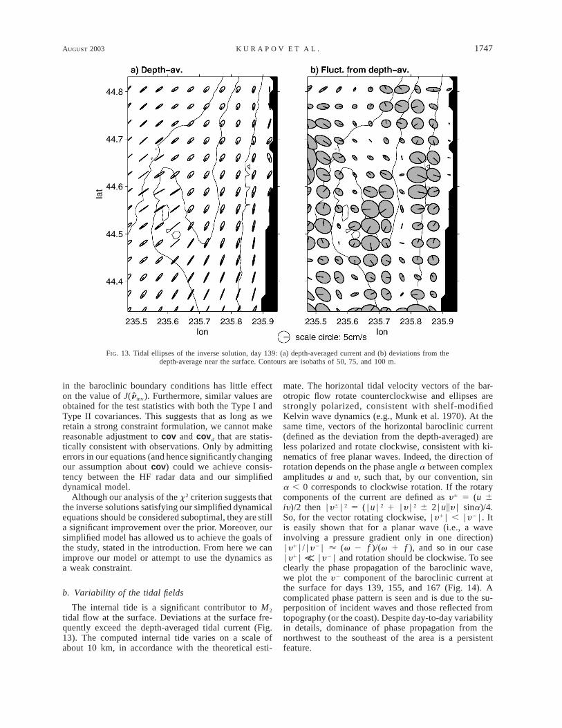
FIG. 13. Tidal ellipses of the inverse solution, day 139: (a) depth-averaged current and (b) deviations from thedepth-average near the surface. Contours are isobaths of 50, 75, and 100 m.

in the baroclinic boundary conditions has little effecton the value of J( inv). Furthermore, similar values arenobtained for the test statistics with both the Type I andType II covariances. This suggests that as long as weretain a strong constraint formulation, we cannot makereasonable adjustment to cov and covd that are statis-tically consistent with observations. Only by admittingerrors in our equations (and hence significantly changingour assumption about cov) could we achieve consis-tency between the HF radar data and our simplifieddynamical model.

Although our analysis of the x2 criterion suggests thatthe inverse solutions satisfying our simplified dynamicalequations should be considered suboptimal, they are stilla significant improvement over the prior. Moreover, oursimplified model has allowed us to achieve the goals ofthe study, stated in the introduction. From here we canimprove our model or attempt to use the dynamics asa weak constraint.

b. Variability of the tidal fields

The internal tide is a significant contributor to M2

tidal flow at the surface. Deviations at the surface fre-quently exceed the depth-averaged tidal current (Fig.13). The computed internal tide varies on a scale ofabout 10 km, in accordance with the theoretical esti-

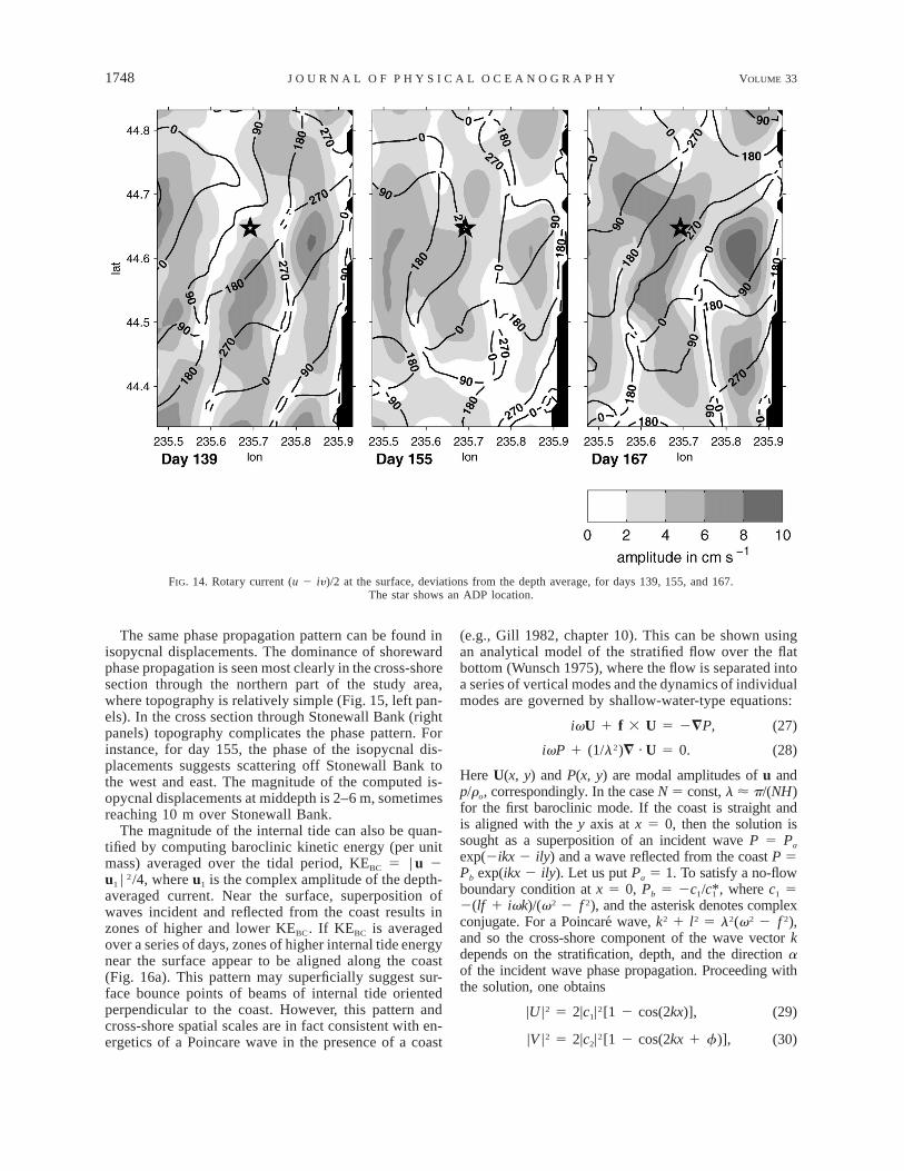
mate. The horizontal tidal velocity vectors of the bar-otropic flow rotate counterclockwise and ellipses arestrongly polarized, consistent with shelf-modifiedKelvin wave dynamics (e.g., Munk et al. 1970). At thesame time, vectors of the horizontal baroclinic current(defined as the deviation from the depth-averaged) areless polarized and rotate clockwise, consistent with ki-nematics of free planar waves. Indeed, the direction ofrotation depends on the phase angle a between complexamplitudes u and y, such that, by our convention, sina , 0 corresponds to clockwise rotation. If the rotarycomponents of the current are defined as y6 5 (u 6iy)/2 then | y6 | 2 5 ( | u | 2 1 | y | 2 6 2 | u\y | sina)/4.So, for the vector rotating clockwise, | y1 | , | y 2 | . Itis easily shown that for a planar wave (i.e., a waveinvolving a pressure gradient only in one direction)| y1 | / | y 2 | ø (v 2 f )/(v 1 f ), and so in our case| y1 | K | y 2 | and rotation should be clockwise. To seeclearly the phase propagation of the baroclinic wave,we plot the y 2 component of the baroclinic current atthe surface for days 139, 155, and 167 (Fig. 14). Acomplicated phase pattern is seen and is due to the su-perposition of incident waves and those reflected fromtopography (or the coast). Despite day-to-day variabilityin details, dominance of phase propagation from thenorthwest to the southeast of the area is a persistentfeature.


FIG. 14. Rotary current (u 2 iy)/2 at the surface, deviations from the depth average, for days 139, 155, and 167.The star shows an ADP location.

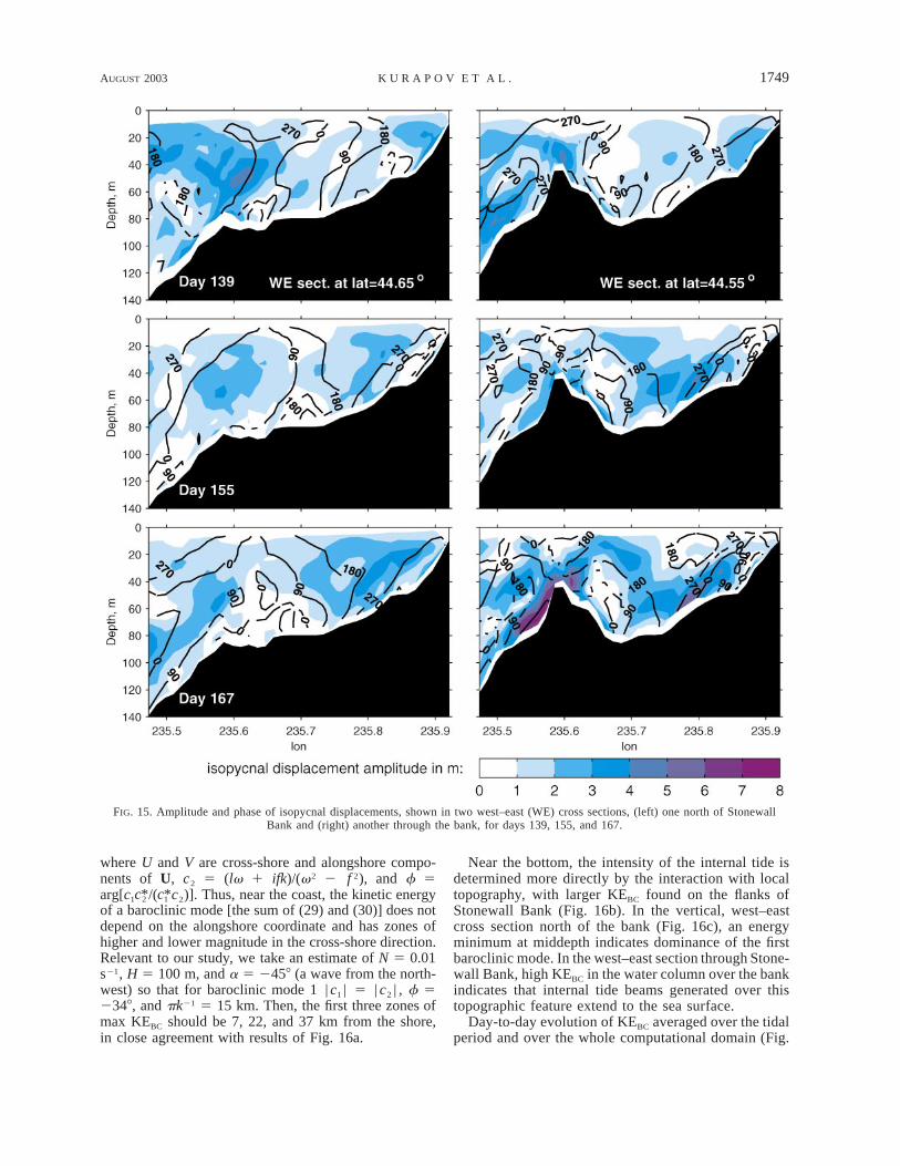
The same phase propagation pattern can be found inisopycnal displacements. The dominance of shorewardphase propagation is seen most clearly in the cross-shoresection through the northern part of the study area,where topography is relatively simple (Fig. 15, left pan-els). In the cross section through Stonewall Bank (rightpanels) topography complicates the phase pattern. Forinstance, for day 155, the phase of the isopycnal dis-placements suggests scattering off Stonewall Bank tothe west and east. The magnitude of the computed is-opycnal displacements at middepth is 2–6 m, sometimesreaching 10 m over Stonewall Bank.

The magnitude of the internal tide can also be quan-tified by computing baroclinic kinetic energy (per unitmass) averaged over the tidal period, KEBC 5 | u 2u1 | 2/4, where u1 is the complex amplitude of the depth-averaged current. Near the surface, superposition ofwaves incident and reflected from the coast results inzones of higher and lower KEBC. If KEBC is averagedover a series of days, zones of higher internal tide energynear the surface appear to be aligned along the coast(Fig. 16a). This pattern may superficially suggest sur-face bounce points of beams of internal tide orientedperpendicular to the coast. However, this pattern andcross-shore spatial scales are in fact consistent with en-ergetics of a Poincare wave in the presence of a coast

(e.g., Gill 1982, chapter 10). This can be shown usingan analytical model of the stratified flow over the flatbottom (Wunsch 1975), where the flow is separated intoa series of vertical modes and the dynamics of individualmodes are governed by shallow-water-type equations:

ivU 1 f 3 U 5 2=P, (27)2ivP 1 (1/l )= · U 5 0. (28)

Here U(x, y) and P(x, y) are modal amplitudes of u andp/ro, correspondingly. In the case N 5 const, l ø p/(NH)for the first baroclinic mode. If the coast is straight andis aligned with the y axis at x 5 0, then the solution issought as a superposition of an incident wave P 5 Pa

exp(2ikx 2 ily) and a wave reflected from the coast P 5Pb exp(ikx 2 ily). Let us put Pa 5 1. To satisfy a no-flowboundary condition at x 5 0, Pb 5 2c1/ , where c1 5c*12(lf 1 ivk)/(v2 2 f 2), and the asterisk denotes complexconjugate. For a Poincare wave, k2 1 l2 5 l2(v2 2 f 2),and so the cross-shore component of the wave vector kdepends on the stratification, depth, and the direction aof the incident wave phase propagation. Proceeding withthe solution, one obtains

2 2|U | 5 2|c | [1 2 cos(2kx)], (29)1

2 2|V | 5 2|c | [1 2 cos(2kx 1 f)], (30)2


FIG. 15. Amplitude and phase of isopycnal displacements, shown in two west–east (WE) cross sections, (left) one north of StonewallBank and (right) another through the bank, for days 139, 155, and 167.

where U and V are cross-shore and alongshore compo-nents of U, c2 5 (lv 1 ifk)/(v2 2 f 2), and f 5arg[c1 /( c2)]. Thus, near the coast, the kinetic energyc* c*2 1

of a baroclinic mode [the sum of (29) and (30)] does notdepend on the alongshore coordinate and has zones ofhigher and lower magnitude in the cross-shore direction.Relevant to our study, we take an estimate of N 5 0.01s21, H 5 100 m, and a 5 2458 (a wave from the north-west) so that for baroclinic mode 1 | c1 | 5 | c2 | , f 52348, and pk21 5 15 km. Then, the first three zones ofmax KEBC should be 7, 22, and 37 km from the shore,in close agreement with results of Fig. 16a.

Near the bottom, the intensity of the internal tide isdetermined more directly by the interaction with localtopography, with larger KEBC found on the flanks ofStonewall Bank (Fig. 16b). In the vertical, west–eastcross section north of the bank (Fig. 16c), an energyminimum at middepth indicates dominance of the firstbaroclinic mode. In the west–east section through Stone-wall Bank, high KEBC in the water column over the bankindicates that internal tide beams generated over thistopographic feature extend to the sea surface.

Day-to-day evolution of KEBC averaged over the tidalperiod and over the whole computational domain (Fig.


FIG. 16. Plot of KEBC averaged over a series of days 139–167: (a) at the surface [contour lines are bathymetry every20 m; red marks show locations of zones of maximum KEBC predicted by the theoretical Poincare wave solution (29)–(30)]; (b) at the bottom; (c) west–east cross section north of Stonewall Bank; and (d) west–east cross section throughStonewall Bank.

FIG. 17. Plot of KEBC averaged over the whole computationaldomain and over the tidal period, shown for a series of days.

17) shows larger values between days 171 and 187,consistent with the impression from Fig. 3. Note thatthe level of KEBC for days 139–147 is the same as fordays 159–167 while both the validation data (see Fig.3a) and the inverse solution at the ADP location (seeFig. 3c) show a lower baroclinic signal for days 139–147 than for days 159–167. This suggests that for days139–147 the baroclinic tide was stronger away from theADP location than near the ADP site, as seen in Fig.14a. So it may be misleading to attempt to assess theintensity of the internal tide in the whole area frominformation collected at one location.

c. Energy balanceUnless the bottom is flat, separation of a flow into

barotropic and baroclinic parts is not obvious, and the


analysis and interpretation of energetics will depend tosome extent on how this partitioning is formally defined.If the barotropic current u1 is defined as the depth av-erage (Cummins and Oey 1997; Holloway 2001), andthe baroclinic current as the deviation from the depthaverage, u2 5 u 2 u1, then the barotropic (depth in-tegrated) energy equation is

] 12 2r (gh 1 H |u | )o 1]t 2

5 2= · (Hu p ) 2 r ru · u(2H ) 2 EC. (31)1 1 o 1

Here the field variables are time-dependent, rather thancomplex amplitudes, p1(x, y, t) is the depth-averaged

pressure, p2(x, y, z, t) 5 p 2 p1, and the first term onthe rhs of (31) is minus the barotropic energy flux di-vergence; EC is the barotropic-to-baroclinic energy con-version rate:

0

cartEC 5 g w r dz, (32)E2H

where wcart is the vertical velocity (aligned with the ver-tical z axis in Cartesian coordinates) associated with thedepth-averaged flow:

z (z 1 H ) ]hcartw 5 u · =H 1 . (33)1H H ]t

The baroclinic, depth-integrated energy equation is

20 0 02] 1 gr ]u2r |u | 1 dz 5 2= · u p dz 2 r ru · u(2H ) 2 r K dz 1 EC, (34)E o 2 E 2 2 o 2 o E M1 2 ) )]t 2 2r ]zz2H 2H 2H

where the first term on the rhs is minus the baroclinicenergy flux divergence. Defining the barotropic and bar-oclinic flows as above has the advantage that the energyconversion term in (31) finds its exact counterpart withopposite sign in (34); adding (31) and (34) yields theenergy equation for the total flow so that the total energyin the model can be accounted for.

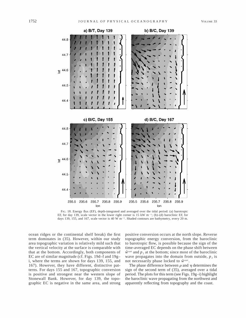
In our analysis, we consider terms in the energy equa-tions averaged over a tidal period. The depth-integratedbarotropic energy flux is from the south to the north(consistent with Kelvin wave dynamics), on the orderof 10 kW m21, with relatively smaller values over theshallows of Stonewall Bank (Fig. 18a). The barotropicflux has low day-to-day variability. The depth-integratedbaroclinic energy flux is much smaller, on the order oftens of watts per meter, and experiences substantial tem-poral variability (Figs. 18b–d). The persistent featurefor all days studied is the general direction of baroclinicenergy flux from northwest to southeast, close to thedirection of phase propagation. This suggests that thecontinental shelf break slope northwest of the studiedarea may be a generation site of energetic M2 internaltide which can propagate onto the shelf. Internal tidesare probably also generated due west and south of ourcomputational domain, but the steeper slopes in theseareas (Fig. 1a) reflect most of the internal tide energytoward deeper water.

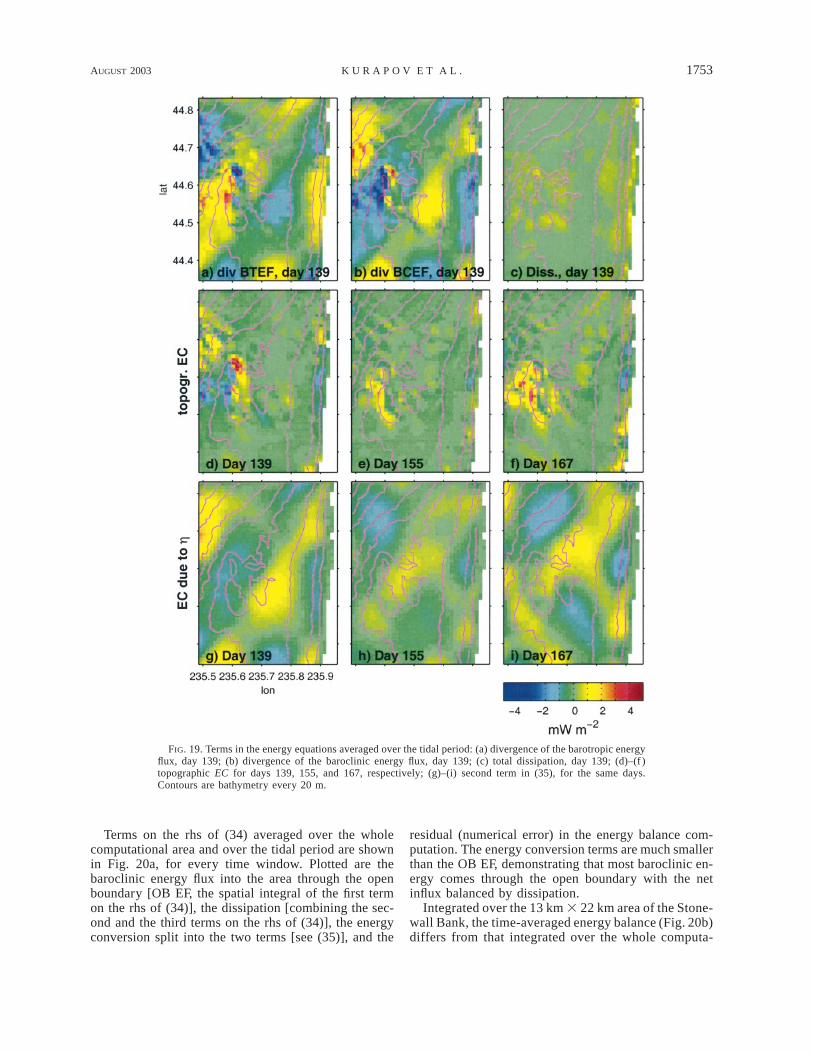
The time-averaged terms in the energy equations forday 139 are shown in Figs. 19a–d and 19g. The diver-gence of the barotropic and baroclinic energy fluxes,and the energy conversion rate, are only a few milliwattsper meter squared, at most. This is several orders ofmagnitude lower than the values seen in areas of stronginternal tide generation such as the Hawaiian Ridge(Merrifield and Holloway 2002). This is partly due to

the shallowness of the area. Also, while the continentalshelf slope outside our domain is steep, we do not expectmuch conversion here compared to Hawaii since bar-otropic flow near the coast mostly follows bathymetriccontours (Baines 1982).

If (33) is substituted into (32), the energy conversionterm can be separated into two parts:

0]h gEC 5 2p | u · =H 1 (z 1 H )r dz, (35)2 z52H 1 E]t H

2H

where the first term is the topographic energy conver-sion (e.g., see Llewellyn-Smith and Young 2001). Thesecond term is associated with sea surface variations,and its physical interpretation is not entirely intuitive.Its appearance is the consequence of our approximatedivision into barotropic (depth averaged) and baroclinicflows, with the elevation and density variations attri-buted solely to the barotropic and baroclinic componentsrespectively. Consideration of the classical problem ofinternal waves over a flat bottom with a free surface(Phillips 1966; Wunsch 1975) shows that this divisionis not exactly correct. For that simple analytical casethe flow can be decomposed into a series of verticalmodes such that the depth averages of the baroclinicpressure modes are not identically zero. Potential energyfor both the barotropic (mode 0) and baroclinic (all othermodes) components include contributions from both el-evation and density variations. Since the modes are dy-namically uncoupled [cf. (27)–(28)] there will be nobarotropic to baroclinic energy conversion. In particular,the second term in (35), which is present even over aflat bottom in our approximate treatment, would notappear with a proper division into barotropic and bar-oclinic modes.

In regions of strong bathymetric variation (such as


FIG. 18. Energy flux (EF), depth-integrated and averaged over the tidal period: (a) barotropicEF, for day 139, scale vector in the lower right corner is 15 kW m21; (b)–(d) baroclinic EF, fordays 139, 155, and 167, scale vector is 40 W m21. Shaded contours are bathymetry, every 20 m.

ocean ridges or the continental shelf break) the firstterm dominates in (35). However, within our studyarea topographic variation is relatively mild such thatthe vertical velocity at the surface is comparable withthat at the bottom. Accordingly, both components ofEC are of similar magnitude (cf. Figs. 19d–f and 19g–i, where the terms are shown for days 139, 155, and167). However, they have different, distinctive pat-terns. For days 155 and 167, topographic conversionis positive and strongest near the western slope ofStonewall Bank. However, for day 139, the topo-graphic EC is negative in the same area, and strong

positive conversion occurs at the north slope. Reversetopographic energy conversion, from the baroclinicto barotropic flow, is possible because the sign of thetime-averaged EC depends on the phase shift betweenwcart and p 2 at the bottom; since most of the baroclinicwave propagates into the domain from outside, p 2 isnot necessarily phase locked to wcart .

The phase difference between r and h determines thesign of the second term of (35), averaged over a tidalperiod. The plots for this term (see Figs. 19g–i) highlightthe baroclinic wave propagating from the northwest andapparently reflecting from topography and the coast.


FIG. 19. Terms in the energy equations averaged over the tidal period: (a) divergence of the barotropic energyflux, day 139; (b) divergence of the baroclinic energy flux, day 139; (c) total dissipation, day 139; (d)–(f )topographic EC for days 139, 155, and 167, respectively; (g)–(i) second term in (35), for the same days.Contours are bathymetry every 20 m.

Terms on the rhs of (34) averaged over the wholecomputational area and over the tidal period are shownin Fig. 20a, for every time window. Plotted are thebaroclinic energy flux into the area through the openboundary [OB EF, the spatial integral of the first termon the rhs of (34)], the dissipation [combining the sec-ond and the third terms on the rhs of (34)], the energyconversion split into the two terms [see (35)], and the

residual (numerical error) in the energy balance com-putation. The energy conversion terms are much smallerthan the OB EF, demonstrating that most baroclinic en-ergy comes through the open boundary with the netinflux balanced by dissipation.

Integrated over the 13 km 3 22 km area of the Stone-wall Bank, the time-averaged energy balance (Fig. 20b)differs from that integrated over the whole computa-


FIG. 20. Terms in the baroclinic energy equation (34) averagedover the tidal period and (a) averaged over the whole computationaldomain, or (b) averaged over the area of the Stonewall Bank. Caselon(HF) , 235.88E. Dots show the residual (numerical error) in theenergy balance.

tional domain (Fig. 20a). Over the bathymetric rise,topographic EC is comparable to the energy flux intothe smaller area and is biased toward positive values.

8. Summary

Our study is the first attempt to model superinertialinternal tide variability on the shelf using data assim-ilation. Since the tidal flow depends critically on hy-drography and open boundary currents that are poorlyknown, data assimilation seems a promising ap-proach. The representer solution and computationswith synthetic data show that in principle measure-ments of surface currents can be used to map tidalflow at depth. For the superinertial M 2 tide, infor-mation from the surface is projected in space alongwave characteristics. Application of our frequencydomain inverse model to HF radar data harmonicallyanalyzed in a series of overlapping 2-week windowsprovides a uniquely detailed picture of the temporaland spatial variability of internal tide on the central

Oregon shelf. Comparison with the ADP data showsthat assimilation of harmonically analyzed surfacecurrent measurements from the coast-based HF radarscaptures temporal variability, as well as variability inthe vertical, of the internal tide.

Although M 2 baroclinic flows on the mid–Oregonshelf are variable and intermittent, some features arefound to be persistent. For instance, during the studyperiod the phase and energy of the baroclinic tide prop-agated in the same direction, from north-west to south-east. At the surface, baroclinic surface tidal currents(deviations from the depth-averaged current) can be 10cm s21 , 2 times as large as the depth-averaged current.Allowing for spring–neap variations and more rapidchanges in the internal tide in response to changes inocean conditions, peak baroclinic velocities in thesemidiurnal band could be easily 2 times this. Theanalysis of the energy balance demonstrates that mostbaroclinic signal comes into the study area via the openboundaries, and so a proper specification of OB con-ditions is critical.

The generalized inverse method offers great flexi-bility in the formulation of the DA problem. For in-stance, weak constraint DA (where dynamical equa-tions are assumed to contain error) is used here to findan appropriate covariance for the open boundary con-dition by nesting. Then, strong constraint DA (withexact dynamics) is implemented to estimate openboundary baroclinic currents using the measured sur-face velocities. One of the values of the representermethod is that a dynamically consistent prior error co-variance for the model solution can be computed, ratherthan guessed.

From the perspective of data assimilation, this studyraises important questions concerning open boundaryconditions. Since DA can provide corrections to theboundary values, there is an opportunity to controlradiation by the choice of open boundary conditioncovariance, consistent with the modeled dynamics. Inour study, nesting is adopted as the simplest way toobtain a covariance that should improve wave radia-tion. Computations with synthetic data show that sucha covariance yields an inverse solution superior to thatobtained with the best covariance that we could makeup without nesting.

Although the dynamical model can in principle beused at any frequency, limited accuracy of HF radardata poses difficulties in estimating major tidal con-stituents, other than M 2 , from short time series. OffOregon, S 2 is the second largest tidal constituent withbarotropic tidal magnitude about 40% of M 2 and aperiod (12 h) very close to that of M 2 (12.4 h). TheK1 diurnal tidal frequency is subinertial so that freeinternal waves are not allowed. Tidal signal in HF radarsurface data at the K1 frequency is probably also con-taminated by wind-induced currents due to a diurnalsea breeze (Erofeeva et al. 2003). Tidal studies in the


diurnal band should probably make allowance for thisadditional forcing.

The internal tide inverse solution is sensitive to thebackground stratification and velocity fields. Thesecould possibly be accounted for within the context ofour simple model by means of weak constraint DA.Then careful interpretation of the dynamical errorwould be necessary to avoid confusion in the analysisof the momentum and energy budget. A better ap-proach to improvement of the internal tide predictionwould be to improve the model by allowing for ahorizontally nonuniform background stratification.Such modifications to the model should also includethe background current to geostrophically balancebackground horizontal pressure gradients. Lineari-zation with respect to this new basic state would yielddynamical terms that describe advection of tidal per-turbations by the background currents. Such a modelcould be useful for addressing the question of theeffect of subinertial currents on internal tides, whichremains open. However, as soon as advective termsare included, the task of finding OB conditions thatguarantee a well-posed formulation becomes nontriv-ial (see Bennett 1992, chapter 9). Our example, witha simpler model, shows that finding an appropriateset of OB conditions does not solve all the problemsat the OB if the task is to restore OB inputs by dataassimilation. Attention should thus also be given tothe OB error covariance.

To provide a more realistic background state, acoastal DA system should eventually couple a tidalinverse model and a reliable model of wind-drivencirculation. This would provide a more realistic back-ground state for the tidal model, as well as a frame-work for studying tidal effects on subtidal flows. Oursuccess with inversion of the HF radar data to describethree-dimensional superinertial tidal flow, using sim-ple dynamics, is encouraging for the optimal use ofsurface current measurements with more advancedmodels.

Acknowledgments. The research was supported bythe Office of Naval Research (ONR) Ocean Modelingand Prediction Program under Grant N00014-98-1-0043, and the National Science Foundation underGrant OCE-9819518.

APPENDIX A

Model Solver

The solution strategy for (11)–(14) is to operatewith parts of the discretized model operator as sparsematrices, eliminate u and w, then solve the reducedsize matrix problem by direct factorization. Elimi-nation of variables is accomplished by a series of

small size matrix inversions locally in each verticalcolumn of the computational grid.

To accomplish this, we approximate (11) by1u 5 Cf 2 C r ,u u (A1)

where C u 5 C(G | P),

h1r 5 , (A2)1 2r

and C ø V 21 . For the original continuous equationsthe operator corresponding to V in (11) and its inverseare local in the horizontal coordinates x and y. So, acontinuous analog of (A1) is exactly equivalent to (2).However, discretized on the staggered C grid the Cor-iolis term couples the u and y components of u atneighboring horizontal locations. This destroys theblock structure of V and makes V 21 a full matrix.To avoid this we directly discretized the horizontallylocal inverse operator: {u, y} is first transformed intoy6 5 (u 6 iy )/2 (Lynch et al. 1992; Muccino et al.1997); the momentum equations are decoupled withrespect to y1 and y 2 , so inversion for y6 is performedlocally at each u and y location of the C grid; finally,backward transformation is made to get u. All thesesteps are fixed in the matrix C.

From (13), we obtain, taking (A1) into account,21 21 21 1w 5 W f 2 W DCf 1 W DC r .w u u (A3)

The resulting system of equations for r1 is obtained bysubstitution of (A1) and (A3) into (12) and (14) andthen combining them to give

1Ar 5 F f 1 F f 1 f ,u wu w r1 (A4)

where

iv I 0A 5 B 1 D C , B 5 ,2 2 2u )1 20 B

DaD 5 2 ,2 211 2D 2 Z W Dr r

0F 5 D C, F 5 ,u 2 w 211 22Z Wr

faf 5 .1r 1 2fr

The matrix B2 is partitioned into blocks such that stan-dard block-matrix multiplication can be performed forB2 and r1 (A2); Fw has zeros in the rows correspondingto the depth-integrated continuity equation. The solutionto (A4) is found by direct LU factorization of A usinga standard routine for banded matrices (Anderson et al.1992). Then multiplication by both A21 and its complexconjugate, matrix transpose (A9)21 can be accomplishedrapidly by solving the appropriate triangular systems.Last, the solution to (11)–(14) is


21 21 21C 2 C A F 2C A F 2C A u wu u u

u f u 21 21 21 21 21n [ w 5 C A F 2 W DC C A F 1 W C A f , (A5) u ww w w w

1r f 1 r21 21 21A F A F A u w

where Cw 5 W21DCu, and a 3 3 3 block-matrix isS21. The size of the numerical problem is limited bythe storage required for the LU factors of the bandedmatrix A. The advantage of the solution approach de-scribed above is that once matrix A is factored, a largenumber of representers [see (21)] can be rapidly com-puted as a series of matrix-vector and vector–vectoroperations. Also, the adjoint solver (S9)21 is easily ob-tained as a complex conjugate, matrix transpose of theblock matrix in (A5).

APPENDIX B

Reduced Basis Approach

Let be a data functional corresponding to the assumedl9kobservation from the reduced basis, k 5 1, · · · , K1. Inour study u sample u and y at 34 points on the surface,l9kso K1 5 68. Representers of the reduced basis are com-puted as rk 5 S21cov(S9)21lk. The inverse solution issought in the form

K1

n 5 n 1 b r . (B1)Oinv 0 k kk51

The task is to find the vector b of representer coefficientsbk that yields a minimum of the original cost function(19), which is

ˆJ(n ) 5 b9Rb 1 (d 2 L9n 2 Pb)9inv 0

213 cov (d 2 L9n 2 Pb). (B2)d 0

Here R is the representer matrix of the reduced basis,of size K1 3 K1, with elements Rkn 5 rn; P is of sizel9kK 3 K1 with elements Pkn 5 rn, where are thel9 l9k k

discrete data functionals for actual observations [see(17)], and rn is the representer from the reduced basis.Optimal representer coefficients are found as in Egbertand Erofeeva (2002):

21/2 2 21 21/2ˆb 5 R QL(l 1 L ) V9cov (d 2 L9n ),d 0 (B3)

where the matrices V, L (diagonal), and Q are theresult of singular value decomposition: VLQ9 5s.v.d.{ PR21/2 }.21/2cov d

REFERENCES

Anderson, E., 1992: LAPACK User’s Guide. Philadelphia, 235 pp.Baines, P. G., 1982: On internal tide generation models. Deep-Sea

Res., 29, 307–338.Bennett, A. F., 1992: Inverse Methods in Physical Oceanography.

Cambridge University Press, 346 pp.

——, 2002: Inverse Modeling of the Ocean and Atmosphere. Cam-bridge University Press, 234 pp.

Blumberg, A. F., and G. L. Mellor, 1987: A description of a three-dimensional coastal ocean circulation model. Three-DimensionalCoastal Ocean Models, N. Heaps, Ed., Coastal and EstuarineScience Series, Vol. 4, Amer. Geophys. Union, 1–16.

Bogden, P. S., 2001: The impact of model–error correlation on re-gional data assimilative models and their observational arrays.J. Mar. Res., 59, 831–857.

Cummins, P. F., and L. Y. Oey, 1997: Simulation of barotropic andbaroclinic tides off northern British Columbia. J. Phys. Ocean-ogr., 27, 762–781.

Egbert, G. D., and S. Y. Erofeeva, 2002: Efficient inverse modelingof barotropic ocean tides. J. Atmos. Oceanic Technol., 19, 183–204.

——, A. F. Bennett, and M. G. G. Foreman, 1994: TOPEX/POSEI-DON tides estimated using a global inverse model. J. Geophys.Res., 99 (C12), 24 821–24 852.

Erofeeva, S. Y., G. D. Egbert, and P. M. Kosro, 2003: Tidal currentson the central Oregon shelf: Models, data, and assimilation. J.Geophys. Res., 108, 3148, doi:10.1029/2002JC001615.

Foreman, M. G. G., L. M. Delves, I. Barrodale, and R. F. Henry,1980: On the use of the Proudman–Heaps tidal theorem. Geo-phys. J. Roy. Astron. Soc., 63, 467–478.

Gill, A. E., 1982: Atmosphere–Ocean Dynamics. Academic Press,662 pp.

Hayes, S. P., and D. Halpern, 1976: Observations of internal wavesand coastal upwelling off the Oregon coast. J. Mar. Res., 34,247–267.

Holloway, P. E., 2001: A regional model of the semi-diurnal internaltide on the Australian North West Shelf. J. Geophys. Res., 106,19 625–19 638.

Kivman, G. A., 1997: Weak constraint data assimilation for tides inthe Arctic Ocean. Progress in Oceanography, Vol. 40, Perga-mon, 179–196.

Kosro, P. M., J. A. Barth, and P. T. Strub, 1997: The coastal jet:observations of surface currents over the Oregon continentalshelf from HF radar. Oceanography, 10, 53–56.

Kurapov, A. L., G. D. Egbert, R. N. Miller, and J. S. Allen, 2002:Data assimilation in a baroclinic coastal ocean model: ensemblestatistics and comparison of methods. Mon. Wea. Rev., 130,1009–1025.

Llewellyn Smith, S. G., and E. R. Young, 2001: Conversion of thebarotropic tide. J. Phys. Oceanogr., 32, 1554–1566.

Lynch, D. R., F. E. Werner, D. A. Greenberg, and J. W. Loder, 1992:Diagnostic model for baroclinic, wind-driven and tidal circula-tion in shallow seas. Cont. Shelf Res., 12, 37–64.

Mellor, G. L., 1998: Users’ guide for a three-dimensional, primitiveequation, numerical ocean model. Program in Atmospheric andOceanic Sciences, Princeton University, Princeton, NJ. [Avail-able online at http://www.aos.princeton.edu/WWWPUBLIC/htdocs.pom/.]

Merrifield, M. A., and P. E. Holloway, 2002: Model estimates of M2

internal tide energetics at the Hawaiian Ridge. J. Geophys. Res.,107, 3179, doi:10.1029/2001JC000996.

Muccino, J. C., W. G. Gray, and M. G. G. Foreman, 1997: Calculationof vertical velocity in three-dimensional, shallow water equation,finite element models. Int. J. Numer. Meth. Fluids, 25, 779–802.

Munk, W., F. Snodgrass, and M. Wimbush, 1970: Tides off shore:


Transition from California coastal to deep-sea waters. Geophys.Fluid Dyn., 1, 161–235.

Oke, P. R., J. S. Allen, R. N. Miller, G. D. Egbert, and P. M. Kosro,2002: Assimilation of surface velocity data into a primitive equa-tion coastal ocean model. J. Geophys. Res., 107 (C9), 3122, doi:10.1029/2000JC000511.

Oliger, J., and A. Sundstrom, 1978: Theoretical and practical aspectsof some initial boundary value problems in fluid dynamics. SIAMJ. Appl. Math., 35, 419–446.

Pacanowski, P. C., and S. C. H. Philander, 1981: Parameterization ofvertical mixing in numerical models of tropical oceans. J. Phys.Oceanogr., 21, 1186–1201.

Petruncio, E. T., L. K. Rosenfeld, and J. D. Paduan, 1998: Obser-vations of the internal tide in Monterey Canyon. J. Phys. Ocean-ogr., 28, 1873–1903.

Phillips, O. M., 1996: Dynamics of the Upper Ocean. CambridgeUniversity Press, 261 pp.

Sirkes, Z., and E. Tziperman, 1997: Finite difference of adjointor adjoint of finite difference? Mon. Wea. Rev., 125, 3373–3378.

Smith, R. L., A. Huyer, and J. Fleischbein, 2000: The coastal oceanoff Oregon from 1961 to 2000: Is there evidence of climatechange or only Los Ninos? Progress in Oceanography, Vol. 49,Pergamon, 63–93.

Torgrimson, G. M., and B. M. Hickey, 1979: Barotropic and baro-clinic tides over the continental slope and shelf off Oregon. J.Phys. Oceanogr., 9, 945–961.

Wijesekera, H. W., J. S. Allen, and P. A. Newberger, 2003: Modelingstudy of turbulent mixing over the continental shelf: Comparisonof turbulent closure schemes. J. Geophys. Res., 108, 3103, doi:10.1029/2001JC001234.

Wunsch, C. H., 1975: Internal tides in the ocean. Rev. Geophys. SpacePhys., 13, 167–182.

m internal tide off oregon: inferences from data assimilationpoa/ · the m2 internal tide off...

Documents