lucie montuelle to cite this version
TRANSCRIPT

HAL Id: tel-01109103https://hal.inria.fr/tel-01109103
Submitted on 24 Jan 2015
HAL is a multi-disciplinary open accessarchive for the deposit and dissemination of sci-entific research documents, whether they are pub-lished or not. The documents may come fromteaching and research institutions in France orabroad, or from public or private research centers.
L’archive ouverte pluridisciplinaire HAL, estdestinée au dépôt et à la diffusion de documentsscientifiques de niveau recherche, publiés ou non,émanant des établissements d’enseignement et derecherche français ou étrangers, des laboratoirespublics ou privés.
Inégalités d’oracle et mélangesLucie Montuelle
To cite this version:Lucie Montuelle. Inégalités d’oracle et mélanges. Statistiques [math.ST]. Université Paris-Sud, 2014.Français. �tel-01109103�

École Doctorale de Mathématiques de la régionParis-Sud
Thèse de doctorat
Discipline : Mathématiques
préparée à l’Université Paris Sud par
Lucie Montuelle
Inégalités d’oracle et mélanges
Soutenue le 4 décembre 2014 devant le jury composé de :
M. Olivier Catoni cnrs et ens Paris ExaminateurM. Gilles Celeux Université Paris-Sud ExaminateurM. Serge Cohen cnrs et Synchrotron Soleil InvitéM. Arnak Dalalyan ensae et Université Paris-Est RapporteurM. Gérard Govaert Université de Technologie de Compiègne RapporteurM. Erwan Le Pennec École Polytechnique DirecteurM. Pascal Massart Université Paris-Sud Président

Thèse préparée auDépartement de Mathématiques d’Orsay
Laboratoire de Mathématiques (UMR 8628), Bât. 425Université Paris-Sud91405 Orsay CEDEX

Inégalités d’oracle et mélanges
Ce manuscrit se concentre sur deux problèmes d’estimation de fonction. Pourchacun, une garantie non asymptotique des performances de l’estimateur proposéest fournie par une inégalité d’oracle.
Pour l’estimation de densité conditionnelle, des mélanges de régressions gaus-siennes à poids exponentiels dépendant de la covariable sont utilisés. Le principede sélection de modèle par maximum de vraisemblance pénalisé est appliqué et unecondition sur la pénalité est établie. Celle-ci est satisfaite pour une pénalité propor-tionnelle à la dimension du modèle. Cette procédure s’accompagne d’un algorithmemêlant EM et algorithme de Newton, éprouvé sur données synthétiques et réelles.
Dans le cadre de la régression à bruit sous-gaussien, l’agrégation à poids expo-nentiels d’estimateurs linéaires permet d’obtenir une inégalité d’oracle en déviation,au moyen de techniques pac-bayésiennes. Le principal avantage de l’estimateur pro-posé est d’être aisément calculable. De plus, la prise en compte de la norme infiniede la fonction de régression permet d’établir un continuum entre inégalité exacte etinexacte.
Mots-clefs : Inégalité d’oracle, sélection de modèle, pénalisation, poids exponen-tiels, apprentissage, agrégation, modèles de mélange, maximum de vraisemblance.
3


Oracle inequalities and mixtures
This manuscript focuses on two functional estimation problems. A non asymp-totic guarantee of the proposed estimator’s performances is provided for each prob-lem through an oracle inequality.
In the conditional density estimation setting, mixtures of Gaussian regressionswith exponential weights depending on the covariate are used. Model selection prin-ciple through penalized maximum likelihood estimation is applied and a conditionon the penalty is derived. If the chosen penalty is proportional to the model dimen-sion, then the condition is satisfied. This procedure is accompanied by an algorithmmixing EM and Newton algorithm, tested on synthetic and real data sets.
In the regression with sub-Gaussian noise framework, aggregating linear estima-tors using exponential weights allows to obtain an oracle inequality in deviation,thanks to pac-bayesian technics. The main advantage of the proposed estimator isto be easily calculable. Furthermore, taking the infinity norm of the regression func-tion into account allows to establish a continuum between sharp and weak oracleinequalities.
Keywords : Oracle inequality, model selection, penalization, exponential weight,learning, aggregation, mixture model, maximum likelihood.
5


Remerciements
La reconnaissance est la mémoire du cœur,Andersen.
Mes premiers remerciements vont à Erwan et Serge, qui m’ont accompagnéependant le stage et la thèse. L’enthousiasme de Serge et de l’équipe Ipanema m’adonné envie de poursuivre ma petite aventure dans la recherche pour trois annéessupplémentaires, sous les conseils avisés d’Erwan. Erwan, merci pour ta disponibilité,ton écoute, ton optimisme féroce et la grande liberté que tu m’as laissée durant cesannées, me permettant d’explorer mes envies scientifiques.
Je suis honorée qu’Arnak Dalalyan et Gérard Govaert aient accepté de rapporterma thèse. Les conseils prodigués ont permis d’améliorer ce manuscrit. Je remerciePascal Massart d’avoir assumé la présidence de mon jury, et Olivier Catoni et GillesCeleux d’y avoir gentiment pris part. L’intérêt porté à mes travaux au travers desquestions et réflexions est source de motivation supplémentaire pour poursuivre danscette voie.
Merci Pascal de m’avoir orientée vers Erwan et de m’avoir conseillée quand lebesoin s’en faisait sentir. Je tiens aussi à remercier Élisabeth Gassiat et Jean-FrançoisLe Gall pour l’attention qu’ils m’ont accordée durant le M2. Étudier et travailler àOrsay a été un plaisir ces dernières années grâce aux membres du laboratoire avecqui j’ai pu interagir. Merci à Nathalie Castelle, Christine Keribin, Claire Lacour,Patrick Pamphile, Thanh Mai Pham Ngoc, et tous ceux qui ont pris de leur tempspour assister à ma soutenance et participer avec enthousiasme au pot.
Qu’auraient été ces années sans la bonne ambiance de bureau assurée par Gian-carlo et Simon puis Laure, Lionel, Thierry, Émilien et Zheng ? Merci aussi auxfidèles participants des pauses thé : Tristan, Olivier, Cagri, Élodie, Morzi, Arthur,Vincent(s), Céline, Valérie, Mélina, Alba, Pierre-Antoine, et ceux qui me pardon-neront d’avoir oublié de les nommer. Je suis heureuse d’avoir participé à des confé-rences et écoles d’été mémorables comme Saint-Flour qui m’ont permis d’avoir descompagnons de fortune sympathiques comme Cécile, Benjamin, Baptiste et Erwan,Mélisande et Carole, Sarah et Émilie, Andrés, Sébastien ou Christophe. Ces voyagesn’auraient pu être accomplis si facilement sans l’aide de Katia Evrat, Valérie La-vigne et Catherine Ardin, qui m’ont guidée dans les méandres administratifs. Jetiens aussi à souligner l’efficacité et la gentillesse de Christine Bailleul, NathalieCarrière, Olivier Chaudet et Pascale Starck.
Merci à l’équipe Ipanema du Synchrotron Soleil : Alessandra, Laurianne, Marie-Angélique, Régina, Loïc, Phil, Sebastian et Serge, pour votre accueil chaleureux.
L’accomplissement de cette thèse a été grandement facilité par les sas de décom-pression offerts par les soirées parisiennes avec Nicolas, Vincent, Ugo ou, dans unregistre plus lyrique, Sébastien. Je souhaite exprimer ma gratitude au noyau durd’(ex-)orcéens : Yann, Tony, Adrien, Henri et Jérémie pour leur appui en toute cir-constance et les soirées entre matheux mais loin des maths. Merci aussi aux amisde prépa Gilles, Rémi, Pécu, Schul et à Solenne toujours présents depuis 10 ans etj’espère pour longtemps encore. Enfin je souhaite exprimer toute ma reconnaissanceà François pour son soutien indéfectible, les merveilleux moments passés et tout ceque nous continuons à partager.
7

Merci à ma famille et particulièrement à mes parents pour leurs prouesses culi-naires à l’occasion du pot (et aussi au quotidien !). Vous avez notamment enduré lesdeux semaines de « vacances » estivales en pleine rédaction sans craquer. Pour cetteraison, pour l’éducation que vous vous êtes efforcés de m’offrir, pour votre soutiensans faille, je souhaite vous rendre hommage. Les « hiéroglyphes » qui suivent sontun peu les vôtres. Pour conclure, merci à Clément pour ses petits plats, et tout lereste...
8

Table des matières
Résumés 3
Remerciements 6
1 État de l’art et contributions 111.1 Problème statistique étudié . . . . . . . . . . . . . . . . . . . . . . . 111.2 Méthodes d’estimation . . . . . . . . . . . . . . . . . . . . . . . . . . 121.3 Oracle, inégalité d’oracle et adaptation . . . . . . . . . . . . . . . . . 141.4 Sélection et agrégation . . . . . . . . . . . . . . . . . . . . . . . . . . 15
1.4.1 Sélection . . . . . . . . . . . . . . . . . . . . . . . . . . . . . . 151.4.2 Agrégation . . . . . . . . . . . . . . . . . . . . . . . . . . . . . 16
1.5 Sélection par contraste pénalisé pour les mélanges gaussiens . . . . . 181.5.1 Estimation par des mélanges gaussiens . . . . . . . . . . . . . 181.5.2 Estimation par des mélanges de régressions gaussiennes à poids
variables . . . . . . . . . . . . . . . . . . . . . . . . . . . . . . 191.5.3 Ma contribution . . . . . . . . . . . . . . . . . . . . . . . . . . 20
1.6 Agrégation PAC-bayésienne à poids exponentiels . . . . . . . . . . . . 201.6.1 Agrégation d’estimateurs . . . . . . . . . . . . . . . . . . . . . 201.6.2 Ma contribution . . . . . . . . . . . . . . . . . . . . . . . . . . 21
2 Mixture of Gaussian regressions model with logistic weights, a pe-nalized maximum likelihood approach 232.1 Framework . . . . . . . . . . . . . . . . . . . . . . . . . . . . . . . . . 242.2 A model selection approach . . . . . . . . . . . . . . . . . . . . . . . 27
2.2.1 Penalized maximum likelihood estimator . . . . . . . . . . . . 272.2.2 Losses . . . . . . . . . . . . . . . . . . . . . . . . . . . . . . . 282.2.3 Oracle inequality . . . . . . . . . . . . . . . . . . . . . . . . . 28
2.3 Mixtures of Gaussian regressions and penalized conditional densityestimation . . . . . . . . . . . . . . . . . . . . . . . . . . . . . . . . . 292.3.1 Models of mixtures of Gaussian regressions . . . . . . . . . . . 292.3.2 A conditional density model selection theorem . . . . . . . . . 302.3.3 Linear combination of bounded functions for the means and
the weights . . . . . . . . . . . . . . . . . . . . . . . . . . . . 322.4 Numerical scheme and numerical experiment . . . . . . . . . . . . . . 33
2.4.1 The procedure . . . . . . . . . . . . . . . . . . . . . . . . . . . 332.4.2 Simulated data sets . . . . . . . . . . . . . . . . . . . . . . . . 352.4.3 Ethanol data set . . . . . . . . . . . . . . . . . . . . . . . . . 37

Table des matières
2.4.4 ChIP-chip data set . . . . . . . . . . . . . . . . . . . . . . . . 402.5 Discussion . . . . . . . . . . . . . . . . . . . . . . . . . . . . . . . . . 412.6 Appendix : A general conditional density model selection theorem . . 422.7 Appendix : Proofs . . . . . . . . . . . . . . . . . . . . . . . . . . . . . 44
2.7.1 Proof of Theorem 1 . . . . . . . . . . . . . . . . . . . . . . . . 442.7.2 Lemma Proofs . . . . . . . . . . . . . . . . . . . . . . . . . . . 472.7.3 Proof of the key proposition to handle bracketing entropy of
Gaussian families . . . . . . . . . . . . . . . . . . . . . . . . . 542.7.4 Proofs of inequalities used for bracketing entropy’s decompo-
sition . . . . . . . . . . . . . . . . . . . . . . . . . . . . . . . . 592.7.5 Proofs of lemmas used for Gaussian’s bracketing entropy . . . 60
2.8 Appendix : Description of Newton-EM algorithm . . . . . . . . . . . 63
3 PAC-Bayesian aggregation of linear estimators 653.1 Introduction . . . . . . . . . . . . . . . . . . . . . . . . . . . . . . . . 653.2 Framework and estimate . . . . . . . . . . . . . . . . . . . . . . . . . 673.3 A general oracle inequality . . . . . . . . . . . . . . . . . . . . . . . . 683.4 Proof of the oracle inequalities . . . . . . . . . . . . . . . . . . . . . . 723.5 The expository case of Gaussian noise and projection estimates . . . . 73
3.5.1 Proof of Lemma 13 . . . . . . . . . . . . . . . . . . . . . . . . 743.5.2 Proof of Theorem 4 . . . . . . . . . . . . . . . . . . . . . . . . 76
3.6 Appendix : Proofs in the sub-Gaussian case . . . . . . . . . . . . . . 783.6.1 Proof of Theorem 3 . . . . . . . . . . . . . . . . . . . . . . . . 783.6.2 Proof of Lemma 14 . . . . . . . . . . . . . . . . . . . . . . . . 79
Bibliography 83
10

Chapitre 1
État de l’art et contributions
Sommaire1.1 Problème statistique étudié . . . . . . . . . . . . . . . . . 11
1.2 Méthodes d’estimation . . . . . . . . . . . . . . . . . . . . 12
1.3 Oracle, inégalité d’oracle et adaptation . . . . . . . . . . 14
1.4 Sélection et agrégation . . . . . . . . . . . . . . . . . . . . 15
1.4.1 Sélection . . . . . . . . . . . . . . . . . . . . . . . . . . . 15
1.4.2 Agrégation . . . . . . . . . . . . . . . . . . . . . . . . . . 16
1.5 Sélection par contraste pénalisé pour les mélanges gaus-
siens . . . . . . . . . . . . . . . . . . . . . . . . . . . . . . . 18
1.5.1 Estimation par des mélanges gaussiens . . . . . . . . . . . 18
1.5.2 Estimation par des mélanges de régressions gaussiennes àpoids variables . . . . . . . . . . . . . . . . . . . . . . . . 19
1.5.3 Ma contribution . . . . . . . . . . . . . . . . . . . . . . . 20
1.6 Agrégation PAC-bayésienne à poids exponentiels . . . . 20
1.6.1 Agrégation d’estimateurs . . . . . . . . . . . . . . . . . . 20
1.6.2 Ma contribution . . . . . . . . . . . . . . . . . . . . . . . 21
1.1 Problème statistique étudié
Le fil conducteur de cette thèse est l’estimation d’une fonction θ0 à partir decouples indépendants de données ((Xi, Yi))1≤i≤n. Diverses méthodes peuvent êtreutilisées pour résoudre ce problème statistique. Dans ce panel, il est souhaitable dechoisir celle qui fournit la meilleure estimation. Cependant, ce choix dépend de laloi des données, rendant l’optimum inconnu. Le but devient alors l’imitation desperformances de la meilleure méthode, en s’adaptant aux données. Cela est garantipar un résultat théorique non asymptotique, appelé inégalité d’oracle.
Le problème envisagé ici a été décliné sous deux formes. La première est l’esti-mation de densité conditionnelle. Y a pour densité θ0 conditionnellement à X parrapport à la mesure de Lebesgue. La question posée est celle du choix du meilleurestimateur parmi des mélanges de régressions gaussiennes dont les poids exponen-tiels dépendent de la covariable X. Elle fait l’objet du chapitre 2. Le second cadre

Chapitre 1. État de l’art et contributions
considéré est l’estimation de fonction de régression, dans un modèle sous-gaussienà design fixe : Y = θ0(X) + W . Ce problème est lié au précédent lorsque la loidu bruit W est connue : un estimateur de la densité conditionnelle peut alors êtrefacilement obtenu à partir de l’estimateur de la fonction de régression. Dans le casdu bruit sous-gaussien, l’estimateur étudié est une moyenne pondérée d’estimateurspar projection des données. Se pose alors la question du choix de ces poids pourl’obtention d’un estimateur aussi performant que la meilleure des projections. Unestratégie est proposée dans le chapitre 3.
En préambule à ces deux objectifs, ce chapitre présente quelques méthodes d’es-timation classiques dans les deux cadres considérés, précise le sens de meilleureestimation ainsi que le type de résultat espéré, une inégalité d’oracle. Deux stra-tégies courantes d’adaptation au meilleur estimateur sont exposées, la sélection etl’agrégation, avant d’être détaillées dans les cadres étudiés. Enfin, mon apport estprécisé pour chacun de ces deux problèmes.
1.2 Méthodes d’estimation
De nombreux estimateurs peuvent être employés pour estimer une fonction derégression ou une densité conditionnelle [voir Wasserman, 2004]. Le problème de l’es-timation de densité conditionnelle a été introduit à la fin des années 60 par Rosen-blatt [1969], qui estime alors la loi jointe du couple (X, Y ) ainsi que la loi marginaleen X à l’aide de noyaux avant d’en faire le quotient. A la même époque, Nadaraya[1965] et Watson [1964] proposent l’estimation de la fonction de régression à l’aidede noyaux. Une revue de la littérature sur cet estimateur est disponible notammentdans le livre de Györfi et al. [2002], qui couvre l’estimation non paramétrique de lafonction de régression. Les estimateurs à noyaux ont été depuis largement étudiés[voir Tsybakov, 2009]. Pour l’estimation de densité conditionnelle, peu de référencessemblent exister avant le milieu des années 90 et la correction par Hyndman et al.[1996] du biais de l’estimateur proposé par Rosenblatt. Des propriétés de convergenceponctuelle des estimateurs localement polynomiaux (Fan et al. [1996], De Gooijerand Zerom [2003] pour la densité conditionnelle et Stone [1982] pour la régressionqui montre aussi la convergence en moyenne quadratique), ou localement logistiques[Hall et al., 1999, Hyndman and Yao, 2002] ont été obtenues et souvent étendues àdes données corrélées. Le livre de Fan and Gijbels [1996] passe en revue les propriétésdes estimateurs par polynômes locaux et propose des critères de choix de fenêtre,notamment dans le cadre de la régression.
Cependant, pour l’obtention de résultats, le choix de la largeur de fenêtre estcrucial mais dépend de la régularité de la fonction à estimer. En pratique, ce choixest rarement discuté, aux exceptions notables de Bashtannyk and Hyndman [2001],Fan and Yim [2004], Hall et al. [2004]. Li and Racine [2007] proposent une explicationdétaillée des méthodes possibles. van Keilegom and Veraverbeke [2002] ont considérédes extensions au cas de données censurées. Enfin Tsybakov [2009] passe en revuel’ensemble des méthodes d’estimation non paramétrique.
Parmi les méthodes non-paramétriques, les projections dans des bases de Fourier,trigonométriques, d’ondelettes [Donoho et al., 1995], ou de splines [Wahba, 1990] sontcouramment utilisées. Ces approches ont les mêmes propriétés que les estimateurs à
12

1.2. Méthodes d’estimation
noyaux, où l’ordre de la série joue le rôle de fenêtre. Ces estimateurs atteignent lesvitesses minimax en régression pour le risque quadratique sur les espaces de Sobolev[Tsybakov, 2009].
Délaissant les noyaux, Stone [1994] propose une modélisation paramétrique dela densité conditionnelle. Il étudie l’estimateur du maximum de vraisemblance basésur des splines. Cette idée a été reprise par Györfi and Kohler [2007] avec une ap-proche par histogramme, Efromovich [2010] par base de Fourier, et Brunel et al.[2007] et Akakpo and Lacour [2011] par une représentation polynomiale par mor-ceaux. Ces auteurs contrôlent une erreur intégrée : une perte intégrée en variationtotale pour le premier et une perte quadratique pour les autres. Brunel et al. [2007]proposent une extension aux données censurées et Akakpo and Lacour [2011] auxdonnées faiblement dépendantes. Blanchard et al. [2007] reprennent l’idée du maxi-mum de vraisemblance dans un cadre de classification à l’aide d’estimateurs parhistogrammes, alors que Cohen and Le Pennec [2013] l’appliquent à l’estimation pardes polynômes par morceaux.
Stone [1994] applique aussi sa méthode au cas de la régression avec l’estimateurdes moindres carrés pour lequel il obtient des résultats similaires à ceux obtenus pourl’estimation de densité conditionnelle, pour la perte quadratique intégrée. L’estima-teur des moindres carrés a été le premier introduit pour l’estimation de régressionpar Gauss et Legendre [1805] pour la détermination des orbites des comètes. Il adepuis été largement utilisé et étudié, notamment dans le cadre des modèles linéairesgénéralisés [McCullagh and Nelder, 1983]. Lorsque les erreurs sont gaussiennes, c’estun cas particulier d’estimateur du maximum de vraisemblance. Des versions régu-larisées de cet estimateur ont été proposées comme le lasso [Tibshirani, 1994], oul’estimateur ridge [Hastie et al., 2009]. Il a été prouvé dans différents cadres que leminimiseur du risque empirique (moins log-vraisemblance ou moindres carrés) a unrisque optimal à constante près au sens minimax pour un choix adéquat de modèle[voir Massart and Nédélec, 2006].
Qualité de l’estimation La qualité de ces estimateurs peut être mesurée par unemesure de dissimilarité, comme la norme ℓ2 ou la divergence de Kullback-Leibler.Pour simplifier, considérons le cas de l’erreur quadratique intégrée, le même phéno-mène se produisant avec la divergence de Kullback-Leibler. Soit θ un estimateur dela fonction θ0. Son erreur quadratique intégrée se décompose comme suit :
E[‖θ − θ0‖2
]=∫
(E [θ(x)] − θ0(x))2 dµ(x) +∫
E[|θ(x) − E [θ(x)] |2
]dµ(x)
=∫biais(θ(x))2dµ(x) +
∫V ar(θ(x))dµ(x).
Un compromis entre le biais et la variance doit donc être établi afin de minimiserle risque de l’estimateur. Celui-ci peut être illustré par l’exemple de la régressiongaussienne homoscédastique à design fixe : Y = θ0 + W , dans lequel les calculsse font aisément. Considérons les estimateurs θm = AmY où Am est la matrice deprojection orthogonale sur l’espace vectoriel Sm. Alors
E[‖θm − θ0‖2
]= ‖Amθ0 − θ0‖2 + E
[‖AmW‖2
]= ‖Amθ0 − θ0‖2 + σ2tr(A⊤
mAm)
= ‖Amθ0 − θ0‖2 + σ2 dim(Sm).
13

Chapitre 1. État de l’art et contributions
Si l’espace Sm est de grande dimension, le biais sera faible mais la variance im-portante. Inversement, si notre choix se porte sur un estimateur par projection surun espace de petite dimension, la variance sera faible mais l’erreur d’estimationsera grande. Un équilibre doit être trouvé. Cependant, ce compromis dépend de lafonction à estimer. Il est donc nécessaire de construire une procédure adaptative.
1.3 Oracle, inégalité d’oracle et adaptation
Les estimateurs présentés ci-dessus ont chacun des qualités qui permettent d’es-pérer une bonne estimation à partir de cette collection sans rien supposer sur lafonction à estimer. L’un des estimateurs va réaliser le risque minimal sur la collec-tion. Or la connaissance de ce risque suppose l’accès à la fonction θ0 inconnue.
La qualité de l’estimation est évaluée par une perte ℓ dont l’espérance est le risqueR. La perte et le risque choisis sont adaptés au contexte. Ainsi, pour l’estimation dedensité conditionnelle, la divergence de Kullback-Leibler mesure l’erreur alors quel’erreur quadratique intégrée, portée par la norme ℓ2, lui a été préférée en régression.De cette façon, selon le cadre étudié, ℓ(θ0, θ) peut être ln θ0 − ln θ ou ‖θ0 − θ‖2.Remarquons que si θ est un estimateur basé sur les données, R(θ0, θ) est une variablealéatoire. Pour souligner cette dépendance, Θn désignera l’ensemble des estimateurscandidats, notés θn.
Oracle Le meilleur estimateur θ⋆n de θ0 parmi l’ensemble des candidats Θn est
celui qui minimise le risque R(θ0, θn) :
θ⋆n ∈ arg min
θn∈Θn
R(θ0, θn).
Cependant, il dépend de la loi des données, qui est inconnue. Il est donc inaccessible,mais son risque peut servir de référence. Cet estimateur idéal est appelé oracle, selonla terminologie introduite par Donoho and Johnstone [1998].
Inégalité d’oracle Bien que l’oracle soit inconnu, il est possible de construire unestimateur θn qui mime ses performances en terme de risque. Cela peut être garantidans le cadre asymptotique par l’optimalité asymptotique :
R(θ0, θn)infθn∈Θn R(θ0, θn)
p.s−−−−→n→+∞
1.
Nous nous sommes concentrés sur le cadre non-asymptotique, où la garantie théo-rique est une inégalité d’oracle :
R(θ0, θn) ≤ Cn infθn∈Θn
R(θ0, θn) + ǫn,
où Cn ≥ 1 est une quantité déterministe bornée et ǫn > 0 est un terme résiduel,souvent négligeable devant infθn∈Θn R(θ0, θn). Lorsque Cn vaut 1, l’inégalité est diteexacte et θn imite l’oracle sur Θn en terme de risque. Cette situation est particuliè-rement intéressante puisqu’elle permet d’évaluer la vitesse minimax. Si Cn > 1 pour
14

1.4. Sélection et agrégation
tout n, l’estimateur imite seulement la vitesse de convergence de l’oracle. L’inégalitéest alors appelée inégalité d’oracle ou inégalité d’oracle approximative. Ces typesd’inégalités peuvent être satisfaits en espérance ou avec grande probabilité. Notonsque θn n’est pas forcément un estimateur de la collection Θn. Les inégalités d’oraclesétablissent des propriétés non asymptotiques d’adaptation à l’oracle et permettentainsi de transférer les propriétés intéressantes de l’oracle.
Adaptation Le problème que nous nous proposons de résoudre peut être énoncécomme suit. Soit ((Xi, Yi))1≤i≤n un ensemble de couples de données indépendants,de loi inconnue liée à la fonction θ0. Soit Θn une collection d’estimateurs construitsà partir des données et θn 7→ R(θ0, θn) un risque pour l’estimation de θ0. Commentconstruire un estimateur θn tel que R(θ0, θn) ≈ infθn∈Θn R(θ0, θn) ou E
[R(θ0, θn)
]≈
infθn∈Θn E[R(θ0, θn)] ?Une première idée consiste à prendre θn dans la collection Θn. C’est la sélection.
Ce choix dur parmi les estimateurs de la collection a l’avantage d’être facilementinterprétable. Cependant, la sélection est peu robuste aux fluctuations, dues aubruit des données. Une légère variation de celles-ci peut mener à la sélection d’unestimateur totalement différent [Yang, 2001]. Vient alors l’idée d’opérer un choixmou, en combinant plusieurs estimateurs de la collection en fonction de la confiancequ’il leur est accordée. Cette stratégie s’appelle l’agrégation.
1.4 Sélection et agrégation
1.4.1 Sélection
Quelques procédures de sélection Plusieurs techniques ont été développéespour sélectionner un modèle, et donc un estimateur. Un panorama de méthodes estdisponible dans l’article de Rao and Wu [2001]. Parmi les plus classiques, citonsla validation croisée [Stone, 1974, Allen, 1974, Geisser, 1975], qui consiste à décou-per le jeu de données en un échantillon d’apprentissage sur lequel les estimateurssont calculés et un échantillon de test permettant d’estimer le risque de chaque es-timateur. Cette technique s’adapte facilement à des contextes variés, mais peu derésultats théoriques sont disponibles (voir Arlot and Celisse [2010] pour un état del’art, Celisse [2008] pour l’estimation de densité et Arlot [2008] pour la régression).Deux autres méthodes usuelles imitent la décomposition biais-variance du risque del’estimateur : la méthode de Goldenshluger and Lepski [2011] et la sélection parcontraste pénalisé. Mentionnons aussi la sélection par test d’hypothèse [Kass andRaftery, 1995, Berger and Pericchi, 1996], qui est intimement liée à l’agrégationbayésienne de modèles [voir Raftery et al., 1997, pour les modèles de régression],avant de détailler la sélection par contraste pénalisé.
Sélection par contraste pénalisé Cette approche a été développée par Barronet al. [1999] (voir aussi Massart [2007]), mais remonte aux années 70, lorsque Akaike[1973] a proposé un critère pénalisé pour la log-vraisemblance dans le cadre del’estimation de densité, l’aic, et Mallows [1973] le critère Cp pour la régression avec
15
Chapitre 1. État de l’art et contributions
les moindres carrés, lorsque la variance des erreurs est supposée connue. Dans lesdeux cas, la pénalité est proportionnelle au nombre de paramètres du modèle. Parla suite, Schwarz [1978] a proposé le bic (pénalisation par le nombre de paramètresdu modèle avec une approche bayésienne), Tibshirani [1994] le lasso (pénalisationpar la norme ℓ1), Tikhonov la pénalisation ridge [Hastie et al., 2009] (pénalisationpar la norme ℓ2), puis est apparu l’elastic net [Zou and Hastie, 2005], mélangeantpénalisation ℓ1 et ℓ2. La pénalisation ℓ1 est arrivée naturellement comme relaxationconvexe de la norme ℓ0, permettant de résoudre le problème de minimisation defaçon efficace d’un point de vue algorithmique.
Pour la sélection par contraste pénalisé, une collection dénombrable M de mo-dèles et un contraste γ sont fixés. Le risque R associé à γ est l’espérance ducontraste selon la loi des données. Plus précisément, si (X, Y ) est un nouveaucouple de données indépendantes des précédentes, tiré selon la même loi, alorsR(θ0, θn) = E[γ(θn, (X, Y )) − γ(θ0, (X, Y ))]. Par exemple, le contraste associé àla divergence de Kullback-Leibler est l’opposé du logarithme. Sur chaque modèle m,un minimiseur θm du risque empirique est construit. L’idée sous-jacente est d’esti-mer sans biais le risque de chaque estimateur. L’estimateur choisi θ est celui associéau modèle qui minimise le contraste empirique pénalisé. En notant γn le contrasteempirique et Θ = {θm,m ∈ M}, l’estimateur sélectionné θ est θm tel que
m ∈ arg infm∈M
{γn(θm) + pen(m)} ,
où pen : M → R+ est la pénalité. Par exemple, pen(m) vaut ln(n)2Dm pour le
bic où Dm est la dimension du modèle m, λ‖θm‖1 pour le lasso, λ‖θm‖22 pour
le ridge et λ1‖θm‖1 + λ2‖θm‖22 pour l’elastic net, avec λ, λ1 et λ2 des paramètres
de régularisation, réels positifs, à calibrer. Remarquons que la pénalisation par lanorme ℓ0 dans une base orthonormée est équivalente au seuillage. Les estimateurspar seuillage sont plus aisément calculables. Des inégalités d’oracle existent pour cesestimateurs ainsi que les autres estimateurs pénalisés précédemment cités [voir entreautres Donoho and Johnstone, 1994, Donoho et al., 1995, Massart, 2007, Massartand Meynet, 2011]
1.4.2 Agrégation
Une alternative à la sélection est l’agrégation. L’estimateur produit n’est plusnécessairement un des estimateurs de la collection Θ, mais une combinaison linéairede ceux-ci. Le problème n’est plus de choisir un estimateur de la collection, maissuite de coefficients. Cette technique générale de génération d’estimateurs adaptatifsest plus puissante que les techniques classiques, puisqu’elle permet de combiner desestimateurs de natures différentes. Cette idée a été étudiée entre autres par Vovk[1990], Littlestone and Warmuth [1994], Cesa-Bianchi et al. [1997], Cesa-Bianchiand Lugosi [1999]. Elle est au cœur de procédures telles que le bagging [Breiman,1996], le boosting [Freund, 1995, Schapire, 1990] ou les forêts aléatoires (Amit andGeman [1997] ou Breiman [2001] ; voir plus récemment Biau et al. [2008], Biau andDevroye [2010], Biau [2012], Genuer [2011]) dont les performances expérimentalessont reconnues.
16

1.4. Sélection et agrégation
Le cadre général de l’agrégation est détaillé par Nemirovski [2000] et étendu dansles livres de Catoni [2004, 2007] par une approche PAC-Bayésienne, ainsi que les tra-vaux de Yang [2000c,b,a, 2001, 2003, 2004a,b]. Enfin Tsybakov [2008] en dresse unpanorama. Dans le cadre de la régression, Tsybakov [2003] a introduit la notion devitesse optimale d’agrégation pour les familles finies d’estimateurs, liée à des inégali-tés d’oracle en espérance, et proposé des procédures les atteignant pour l’agrégationlinéaire, convexe et l’agrégation de type sélection de modèle. Lounici [2007], Rigolletand Tsybakov [2007], Rigollet [2006] ainsi que Lecué [2007] se sont penchés sur cesproblèmes en régression ou pour l’estimation de densité. Remarquons que le choixdes coefficients d’agrégation peut être fait en utilisant les méthodes de sélection parcontraste pénalisé précédentes avec la perte quadratique. Par exemple, l’estimateurbic atteint les vitesses optimales pour les problèmes précédents [voir Bunea et al.,2007] tout comme le lasso pour le problème de sélection [Massart and Meynet,2011].
Cependant, les estimateurs candidats sont « gelés » dans ces travaux : soit ilssont déterministes, soit ils sont construits à partir d’un échantillon indépendant decelui utilisé pour l’agrégation. Cette hypothèse a été levée par Leung and Barron[2006] qui ont obtenu la première inégalité d’oracle exacte en espérance en agré-geant des projections à l’aide de poids exponentiels, dans le cadre de la régressiongaussienne. Ces résultats ont été étendus à un bruit plus général et une famille nondénombrable d’estimateurs potentiellement gelés par Dalalyan and Tsybakov [2007,2008, 2012]. Ces derniers résultats ont été obtenus à l’aide de poids exponentiels, quisont un exemple important d’agrégation (voir Rigollet and Tsybakov [2012] pour unhistorique récent).
Agrégation à poids exponentiels L’agrégation à poids exponentiels se justified’un point de vue quasi-bayésien dans le cadre de la régression à design déterministe
Yi = θ0(xi) + ξi,
avec les ξi indépendants de loi normale centrée de variance σ2. Supposons la va-riance connue et qu’un dictionnaire de fonctions déterministes {θ1, . . . , θM} est ànotre disposition. L’estimateur agrégé à poids exponentiels peut alors être vu commel’estimateur de Bayes dans le modèle fantôme
Yi =M∑
j=1
wjθj(xi) + ξ′i,
où wj ≥ 0, les ξ′i sont indépendants de loi normale centrée de variance β
2, et la
loi a priori porte sur les vecteurs de la base canonique de RM . Ce n’est que quasibayésien car en général, θ0 n’est pas une combinaison linéaire des θj et le réel β doitêtre supérieur à 4σ2 pour l’obtention d’inégalités oracles.
L’agrégation à poids exponentiels peut aussi être vue comme une approximationde la sélection des coefficients par minimisation de risque empirique pénalisé. Lapénalité employée est la divergence de Kullback-Leibler, favorisant ainsi les distri-butions proches de la loi a priori, et le contraste est associé à la perte quadratique. Ceproblème de minimisation est en général dur à résoudre, c’est pourquoi le risque qua-dratique de l’estimateur agrégé est majoré par la combinaison convexe des risques de
17

Chapitre 1. État de l’art et contributions
chaque élément du dictionnaire. Les poids exponentiels sont solution de ce nouveauproblème de minimisation sur tous les poids dans le simplexe.
Cette propriété leur a valu d’être largement utilisés pour l’obtention d’inégali-tés d’oracle via les résultats PAC-bayésiens. L’approche Probably ApproximatelyCorrect est employée dans ce contexte pour contrôler en probabilité le risque théo-rique par le risque empirique pour toute mesure. La technique PAC a été initiée parShawe-Taylor and Williamson [1997] et McAllester [1998], et améliorée par Seeger[2003] dans le cas des processus gaussiens. Elle a été étendue par Catoni [2004] enclassification et en régression avec la perte quadratique où les vitesses atteintes sontoptimales au sens minimax dans certains cas. Audibert [2004] a obtenu les premiersrésultats adaptatifs, suivi de Catoni [2007]. La technique PAC-bayésienne a aussiété élargie à d’autres contextes.
Lorsque des résultats en espérance sont souhaités, l’estimation sans biais durisque via l’estimateur sure de Stein [1981] se substitue aux contrôles de dévia-tions. Pour les estimateurs affines, il est possible sous certaines conditions de ma-jorer l’estimateur sure de l’estimateur agrégé par l’agrégat des estimateurs suredes estimateurs de la collection [voir Leung, 2004, Dalalyan and Salmon, 2012]. Lapénalisation par la divergence de Kullback-Leibler entre la mesure d’agrégation etla loi a priori sur la collection d’estimateurs rend les poids exponentiels optimauxet permet d’avoir une solution explicite de ce problème. La divergence de Kullback-Leibler joue le rôle de borne d’union pour la minimisation sur l’ensemble des mesuresd’agrégation.
Voyons maintenant comment la sélection et l’agrégation ont été mises en œuvredans deux contextes particuliers : l’estimation de densité conditionnelle par desmélanges gaussiens et l’estimation de fonction de régression à l’aide d’estimateurslinéaires respectivement.
1.5 Sélection par contraste pénalisé pour les mé-langes gaussiens
1.5.1 Estimation par des mélanges gaussiens
Un modèle couramment utilisé pour l’estimation de densité ou la classificationest le mélange gaussien. Il se présente sous la forme d’une moyenne pondérée dedensités gaussiennes dont les paramètres sont le nombre de composantes, les poidsainsi que les moyennes et variances de chaque composante. Le contraste employé estalors l’opposé du logarithme et la perte associée est la distance de Kullback-Leibler.
La classification a souvent recourt aux pénalisations aic et bic pour le choix dunombre de composantes du mélange [voir Burnham and Anderson, 2002]. Cependant,les heuristiques associées à ces pénalités supposent l’appartenance de la fonctionestimée à la collection de modèles. S’affranchissant de cette hypothèse et s’appuyantsur le travail de Massart [2007], Maugis and Michel [2011] ont fourni une pénalitépermettant d’obtenir une inégalité d’oracle aussi bien pour la sélection du nombrede composantes que des autres paramètres. Ce résultat repose sur le contrôle de lacomplexité de chaque modèle par son entropie à crochets, ainsi que de la collection
18

1.5. Sélection par contraste pénalisé pour les mélanges gaussiens
de modèles par une hypothèse du type inégalité de Kraft.L’entropie à crochets a aussi été employée dans un cadre bayésien pour obtenir
des propriétés asymptotiques de consistance des distributions a posteriori pour lesmélanges gaussiens par Choi [2008], et des vitesses de convergence par Genovese andWasserman [2000] ou van der Vaart and Wellner [1996] lorsque la densité cible estun mélange gaussien.
En présence d’une covariable, il est tentant de complexifier le modèle de mé-lange gaussien en transformant les moyennes constantes en fonctions. Ce modèle estbien documenté (voir McLachlan and Peel [2000]). En particulier, dans le contextebayésien, Viele and Tong [2002] ont majoré des entropies à crochets pour prouverla consistance de la loi a posteriori pour les mélanges de régressions gaussiennes.Dans le cadre paramétrique, Young [2014] utilise des mélanges à poids constantsde gaussiennes dont les moyennes sont des fonctions continues affines par morceaux(nommées regression with changepoints). Il use du maximum de vraisemblance péna-lisé par le bic pour construire un estimateur calculable par un algorithme semblableà l’EM. Une alternative consiste à faire varier les poids en fonction de la cova-riable. En considérant des poids constants par morceaux et en se basant sur uneidée de Kolaczyk et al. [2005], Antoniadis et al. [2009] se sont intéressés à la vi-tesse de convergence de leur estimateur basé sur la log-vraisemblance pénalisée. Ilsont supposé les composantes gaussiennes connues. Cette hypothèse peut être levéepour l’obtention d’une inégalité d’oracle, comme l’ont montré Cohen and Le Pennec[2013]. Ces modèles sont fréquemment utilisés en économétrie [voir Li and Racine,2007].
Des mélanges dans lesquels à la fois les moyennes et les poids dépendent d’unecovariable sont présentés par Ge and Jiang [2006] mais uniquement pour les mélangesde régressions logistiques. Ils donnent des conditions sur le nombre de composantesdu mélange à poids logistiques qui assurent la consistance de la loi a posteriori. Lee[2000] a étudié des propriétés similaires pour les réseaux de neurones.
1.5.2 Estimation par des mélanges de régressions gaussiennesà poids variables
Les mélanges de régressions gaussiennes à poids logistiques ne semblent appa-raître dans la littérature qu’au milieu des années 90. Jordan and Jacobs [1994]proposent un algorithme basé sur l’EM et l’algorithme des moindres carrés pondé-rés (en anglais, Iteratively Reweighted Least Squares) pour estimer les paramètresdu modèle de mélange hiérarchisé d’experts, mais ne font pas d’analyse théorique.Dans ce modèle, les composantes et les poids sont des modèles linéaires générali-sés. Young and Hunter [2010] considèrent un mélange de régressions gaussiennes àpoids variables, pas nécessairement logistiques, estimés par une approche non pa-ramétrique mêlant noyaux et validation croisée. Cette procédure est soutenue pardes simulations à l’aide d’un algorithme proche de l’EM, dont les auteurs com-parent les performances. Ce travail trouve une extension dans [Hunter and Young,2012, Huang and Yao, 2012], où sont considérés des mélanges semi-paramétriquesde régressions, pour lesquels des conditions pour l’identifiabilité et un algorithme si-milaire sont donnés. Huang et al. [2013] proposent une estimation non-paramétrique
19

Chapitre 1. État de l’art et contributions
des moyennes, variances et poids. Ils établissent la normalité asymptotique de l’es-timateur construit à l’aide de noyaux et de validation croisée, et l’accompagnentd’un algorithme. Chamroukhi et al. [2010] proposent des mélanges de régressionspolynomiales par morceaux à poids logistiques pour l’estimation fonctionnelle. Ilssélectionnent un estimateur par maximum de vraisemblance pénalisé par le critèrebic et fournissent un algorithme, mais pas de justification théorique.
1.5.3 Ma contribution
Les simulations encourageantes de Chamroukhi et al. [2009] sur l’estimation defonction par des mélanges à poids logistiques de régressions polynomiales par mor-ceaux, nous ont poussé à chercher une garantie théorique. C’est pourquoi nous avonsconsidéré des mélanges de régressions gaussiennes à poids logistiques. Les travauxde Cohen and Le Pennec [2011] esquissaient la possibilité d’estimer des densitésconditionnelles par de tels mélanges, y compris avec des régressions gaussiennespar morceaux. Tout comme eux, nous avons obtenu une condition sur la pénalitéassurant une inégalité d’oracle en espérance pour l’estimateur sélectionné par maxi-mum de vraisemblance pénalisé. Nous montrons qu’une pénalité proportionnelle àla dimension du modèle convient, ce qui n’avait pas encore été vérifié dans ce cadre.
De plus, la procédure d’estimation est facilement implémentable en combinantles algorithmes EM et de Newton. L’usage de poids logistiques permet une parti-tion souple des données selon la covariable, en autorisant plus d’une régression pourune même valeur de la covariable. Cela se traduit en dimension 1 par des frontièresnon parallèles aux axes entre les différentes classes lors de la représentation gra-phique des données. La question cruciale de l’initialisation de l’algorithme EM a ététraitée dans le cas de moyennes affines avec des données unidimensionnelles. Elledevient beaucoup plus délicate lorsque la dimension des données augmente, la fauteincombant au fléau de la dimension. La procédure que nous proposons a été utiliséepour illustration sur les données de Brinkman [1981] et sur des données génétiquesétudiées par Martin-Magniette et al. [2008]. Les données de Brinkman présententune mesure du mélange air-éthanol utilisé dans le test d’un moteur mono-cylindreet la concentration en monoxyde d’azote des émissions du moteur. L’estimateursélectionné par notre procédure retrouve des phases connues et interprétables dufonctionnement d’un moteur. Dans le jeu de données génétiques, le but est de trou-ver des groupes de protéines accrochées aux brins d’ADN. Ces exemples illustrentl’intérêt des mélanges de régressions à poids logistiques puisqu’ils améliorent l’esti-mation en prenant en compte l’information apportée par la covariable à plusieursniveaux.
1.6 Agrégation PAC-bayésienne à poids exponen-tiels
1.6.1 Agrégation d’estimateurs
Dans la plupart des travaux précédemment cités traitant d’agrégation, les ré-sultats portent sur l’agrégation d’estimateurs « gelés » car l’analyse devient trop
20

1.6. Agrégation PAC-bayésienne à poids exponentiels
complexe, et des astuces de division ou de clonage de l’échantillon [Tsybakov, 2014]sont utilisées. Actuellement, seuls les estimateurs par projection orthogonale [Leung,2004] et les estimateurs affines [Dalalyan and Salmon, 2012] permettent d’estimeret d’agréger à partir du même échantillon sans sur-apprentissage. Cependant, lesinégalités d’oracle obtenues sont en espérance, aux exceptions notables de Audibert[2008] pour les progressive mixture rules, Lecué and Mendelson [2009], Gaïffas andLecué [2011] avec un procédure basée sur la découpe de l’échantillon dans le cas dudesign aléatoire, et Rigollet [2012] pour le design fixe.
Dai et al. [2012] montrent que les poids exponentiels sont sous-optimaux endéviation : l’espérance du risque quadratique intégré est de l’ordre optimal mais pasles déviations autour de l’espérance. Ils corrigent cela pour la régression gaussienneà design fixe en changeant le problème de minimisation dont les poids exponentielssont solution. Ils remplacent le risque empirique de l’estimateur agrégé par unecombinaison convexe du risque de l’estimateur agrégé et l’agrégat des risques desestimateurs du dictionnaire. Pour la régression gaussienne homoscédastique, Daiet al. [2014] ont obtenu une inégalité d’oracle pour les poids exponentiels et uneinégalité d’oracle exacte pour leur nouvelle procédure avec grande probabilité enagrégeant des estimateurs affines.
Les travaux cités en régression supposent la variance connue, aux exceptions deDalalyan and Salmon [2012] et Dalalyan et al. [2013] dans le cadre hétéroscédastique ;et Belloni et al. [2011], Dalalyan [2012], Giraud [2008], Giraud et al. [2012], Sun andZhang [2012] qui se placent dans le cadre homoscédastique.
1.6.2 Ma contribution
Parallèlement à ces travaux, nous avons obtenu une inégalité d’oracle en probabi-lité pour la régression à bruit sous-gaussien en agrégeant des estimateurs linéaires àl’aide de poids exponentiels. L’idée principale consiste à remplacer l’estimateur sansbiais du risque traditionnellement utilisé dans les poids par une version pénalisée. Sila norme infinie de la fonction de régression est connue, l’inégalité oracle peut êtrerendue exacte en prenant en compte le rapport signal sur bruit dans la pénalité. Lelien entre la prise en compte de ce rapport dans la pénalité et le coefficient devantle risque de l’oracle est mis en évidence, établissant un continuum entre inégalitéexacte et inexacte. Remarquons que les poids exponentiels proposés par Dai et al.[2014] utilisent un estimateur biaisé du risque et que nous obtenons la même bornesur la température dans le cas gaussien.
21


Chapter 2
Mixture of Gaussian regressionsmodel with logistic weights, apenalized maximum likelihoodapproach
This chapter is an extended version of the article [Montuelle and Le Pennec,2014], published in Electronic Journal of Statistics.
Sommaire2.1 Framework . . . . . . . . . . . . . . . . . . . . . . . . . . . 24
2.2 A model selection approach . . . . . . . . . . . . . . . . . 27
2.2.1 Penalized maximum likelihood estimator . . . . . . . . . . 27
2.2.2 Losses . . . . . . . . . . . . . . . . . . . . . . . . . . . . . 28
2.2.3 Oracle inequality . . . . . . . . . . . . . . . . . . . . . . . 28
2.3 Mixtures of Gaussian regressions and penalized condi-
tional density estimation . . . . . . . . . . . . . . . . . . . 29
2.3.1 Models of mixtures of Gaussian regressions . . . . . . . . 29
2.3.2 A conditional density model selection theorem . . . . . . 30
2.3.3 Linear combination of bounded functions for the meansand the weights . . . . . . . . . . . . . . . . . . . . . . . . 32
2.4 Numerical scheme and numerical experiment . . . . . . 33
2.4.1 The procedure . . . . . . . . . . . . . . . . . . . . . . . . 33
2.4.2 Simulated data sets . . . . . . . . . . . . . . . . . . . . . 35
2.4.3 Ethanol data set . . . . . . . . . . . . . . . . . . . . . . . 37
2.4.4 ChIP-chip data set . . . . . . . . . . . . . . . . . . . . . . 40
2.5 Discussion . . . . . . . . . . . . . . . . . . . . . . . . . . . . 41
2.6 Appendix : A general conditional density model selec-
tion theorem . . . . . . . . . . . . . . . . . . . . . . . . . . 42
2.7 Appendix : Proofs . . . . . . . . . . . . . . . . . . . . . . . 44
2.7.1 Proof of Theorem 1 . . . . . . . . . . . . . . . . . . . . . 44
2.7.2 Lemma Proofs . . . . . . . . . . . . . . . . . . . . . . . . 47
Bracketing entropy’s decomposition . . . . . . . . . . . . 47

Chapter 2. Mixture of Gaussian regressions with logistic weights
Bracketing entropy of weight’s families . . . . . . . . . . . 49
Bracketing entropy of Gaussian families . . . . . . . . . . 51
2.7.3 Proof of the key proposition to handle bracketing entropyof Gaussian families . . . . . . . . . . . . . . . . . . . . . 54
Proof of Proposition 2 . . . . . . . . . . . . . . . . . . . . 54
2.7.4 Proofs of inequalities used for bracketing entropy’s decom-position . . . . . . . . . . . . . . . . . . . . . . . . . . . . 59
2.7.5 Proofs of lemmas used for Gaussian’s bracketing entropy . 60
Proof of Lemma 9 . . . . . . . . . . . . . . . . . . . . . . 60
Proof of Lemma 10 . . . . . . . . . . . . . . . . . . . . . . 61
Proof of Lemma 11 . . . . . . . . . . . . . . . . . . . . . . 62
2.8 Appendix : Description of Newton-EM algorithm . . . . 63
Abstract In the framework of conditional density estimation, we use candidatestaking the form of mixtures of Gaussian regressions with logistic weights and meansdepending on the covariate. We aim at estimating the number of components ofthis mixture, as well as the other parameters, by a penalized maximum likelihoodapproach. We provide a lower bound on the penalty that ensures an oracle inequal-ity for our estimator. We perform some numerical experiments that support ourtheoretical analysis.
Keywords : Mixture of Gaussian regressions models, Mixture of regressionsmodels, Penalized likelihood, Model selection.
2.1 Framework
In classical Gaussian mixture models, the density is modeled by
sK,υ,Σ,w(y) =K∑
k=1
πw,kΦυk,Σk(y),
where K ∈ N \ {0} is the number of mixture components, Φυ,Σ is the Gaussiandensity with mean υ and covariance matrix Σ,
Φυ,Σ(y) =1√
(2π)p|Σ|e
−12
(y−υ)′Σ−1(y−υ)
and πw,k are the mixture weights, that can always be defined from a K-tuple w =(w1, . . . , wK) with a logistic scheme:
πw,k =ewk
∑Kk′=1 e
wk′.
In this article, we consider such a model in which the mixture weights as well as themeans can depend on a, possibly multivariate, covariate.
More precisely, we observe n pairs of random variables ((Xi, Yi))1≤i≤n where thecovariates Xis are independent while the Yis are conditionally independent giventhe Xis. We assume that the covariates are in some subset X of Rd and the Yis
24

2.1. Framework
are in Rp. We want to estimate the conditional density s0(·|x) with respect to theLebesgue measure of Y given X. We model this conditional density by a mixture ofGaussian regressions with varying logistic weights
sK,υ,Σ,w(y|x) =K∑
k=1
πw(x),kΦυk(x),Σk(y),
where υ = (υ1, . . . , υK) and w = (w1, . . . , wK) are now K-tuples of functions chosen,respectively, in a set ΥK and WK . Our aim is then to estimate those functions υk
and wk, the covariance matrices Σk as well as the number of classes K so that theerror between the estimated conditional density and the true conditional density isas small as possible.
The classical Gaussian mixture case has been extensively studied [McLachlanand Peel, 2000]. Nevertheless, theoretical properties of such model have been lessconsidered. In a Bayesian framework, asymptotic properties of the posterior distri-bution are obtained by Choi [2008], Genovese and Wasserman [2000], van der Vaartand Wellner [1996] when the true density is assumed to be a Gaussian mixture.AIC/BIC penalization scheme are often used to select a number of clusters (seeBurnham and Anderson [2002] for instance). Non asymptotic bounds are obtainedby Maugis and Michel [2011] even when the true density is not a Gaussian mixture.All these works rely heavily on a bracketing entropy analysis of the models, that willalso be central in our analysis.
When there is a covariate, the most classical extension of this model is a mixtureof Gaussian regressions, in which the means υk are now functions. It is well studiedas described in McLachlan and Peel [2000]. In particular, in a Bayesian framework,Viele and Tong [2002] have used bracketing entropy bounds to prove the consistencyof the posterior distribution. Models in which the proportions vary have been con-sidered by Antoniadis et al. [2009]. Using an idea of Kolaczyk et al. [2005], theyhave considered a model in which only proportions depend in a piecewise constantmanner from the covariate. Their theoretical results are nevertheless obtained underthe strong assumption they exactly know the Gaussian components. This assump-tion can be removed as shown by Cohen and Le Pennec [2013]. Models in whichboth mixture weights and means depend on the covariate are considered by Ge andJiang [2006], but in a mixture of logistic regressions framework. They give conditionson the number of components (experts) to obtain consistency of the posterior withlogistic weights. Note that similar properties are studied by Lee [2000] for neuralnetworks.
Although natural, mixture of Gaussian regressions with varying logistic weightsseems to be mentioned first by Jordan and Jacobs [1994]. They provide an algorithmsimilar to ours, based on EM and Iteratively Reweighted Least Squares, for hier-archical mixtures of experts but no theoretical analysis. Young and Hunter [2010]choose a non-parametric approach to estimate the weights, which are not supposedlogistic anymore, using kernels and cross-validation. They also provide an EM-likealgorithm and some convincing simulations. This work has an extension in a seriesof papers [Hunter and Young, 2012], [Huang and Yao, 2012]. Young [2014] considersmixture of regressions with changepoints but constant proportions. More recently,Huang et al. [2013] have considered a non-parametric modeling for the means, the
25

Chapter 2. Mixture of Gaussian regressions with logistic weights
proportions as well as the variance for which they give asymptotic properties as wellas a numerical algorithm. Closer to our work, Chamroukhi et al. [2010] consider thecase of piecewise polynomial regression model with affine logistic weights. In our set-ting, this corresponds to a specific choice for ΥK and WK : a collection of piecewisepolynomials and a set of affine functions. They use a variation of the EM algorithmand a BIC criterion and provide numerical experiments to support the efficiency oftheir scheme.
0 0.5 1 1.5 2 2.5 3 3.5 4 4.50.5
0.6
0.7
0.8
0.9
1
1.1
1.2
1.3
NO
Eq
uiv
ale
nce
Ra
tio
(a) Raw Ethanol data set
0 0.5 1 1.5 2 2.5 3 3.5 4 4.50.4
0.5
0.6
0.7
0.8
0.9
1
1.1
1.2
1.3
NO
Equ
ival
ence
Rat
io
(b) Clustering deduced from the estimated condi-tional density by a MAP principle.
(c) 3D view of the resulting conditional densityshowing the 4 regression components.
(d) 2D view of the same conditional density. Thedifferent variances are visible as well as the con-nectedness of the two topmost clusters.
Figure 2.1 – Estimated density with 4 components based upon the NO data set
Young [2014] provides a relevant example for our analysis. The ethanol data setof Brinkman [1981] (Figure 2.1a) shows the relationship between the equivalenceratio, a measure of the air-ethanol mix used as a spark-ignition engine fuel in asingle-cylinder automobile test, and the engine’s concentration of nitrogen oxide(NO) emissions for 88 tests. Using the methodology described in this paper, weobtain a conditional density modeled by a mixture of four Gaussian regressions.Using a classical maximum likelihood approach, each point of the data set can beassigned to one the four class yielding the clustering of Figure 2.1b. The use of logistic
26

2.2. A model selection approach
weight allows a soft partitioning along the NO axis while still allowing more thanone regression for the same NO value. The two topmost classes seem to correspondto a single population whose behavior changes around 1.7 while the two bottom-most classes appear to correspond to two different populations with a gap around2.6 − 2.9. Such a result could not have been obtained with non varying weights.
The main contribution of our paper is a theoretical result: an oracle inequality,a non asymptotic bound on the risk, that holds for penalty slightly different fromthe one used by Chamroukhi et al. [2010].
In Section 2.2, we recall the penalized maximum likelihood framework, introducethe losses considered and explain the meaning of such an oracle inequality. In Sec-tion 2.3, we specify the models considered and their collections, state our theoremunder mild assumptions on the sets ΥK and WK and apply this result to polynomialsets. Those results are then illustrated by some numerical experiments in Section 2.4.Our analysis is based on an abstract theoretical analysis of penalized maximum like-lihood approach for conditional densities conducted in Cohen and Le Pennec [2011]that relies on bracketing entropy bounds. Appendix 2.6 summarizes those resultswhile Appendix 2.7 contains the proofs specific to this paper, the ones concerningbracketing entropies.
2.2 A model selection approach
2.2.1 Penalized maximum likelihood estimator
We will use a model selection approach and define some conditional density mod-els Sm by specifying sets of conditional densities, taking the shape of mixtures ofGaussian regressions, through their number of classes K, a structure on the covari-ance matrices Σk and two function sets ΥK and WK to which belong respectivelythe K-tuple of means (υ1, . . . , υK) and the K-tuple of logistic weights (w1, . . . , wK).Typically those sets are compact subsets of polynomials of low degree. Within sucha conditional density set Sm, we estimate s0 by the maximizer sm of the likelihood
sm = argmaxsK,υ,Σ,w∈Sm
n∑
i=1
ln sK,υ,Σ,w(Yi|Xi),
or more precisely, to avoid any existence issue since the infimum may not be uniqueor even not be reached, by any η-minimizer of the negative log-likelihood:
n∑
i=1
− ln sm(Yi|Xi) ≤ infsK,υ,Σ,w∈Sm
n∑
i=1
− ln sK,υ,Σ,w(Yi|Xi) + η.
Assume now we have a collection {Sm}m∈M of models, for instance with differentnumber of classes K or different maximum degree for the polynomials defining ΥK
and WK , we should choose the best model within this collection. Using only the log-likelihood is not sufficient since this favors models with large complexity. To balancethis issue, we will define a penalty pen(m) and select the model m that minimizes (orrather η′-almost minimizes) the sum of the negative log-likelihood and this penalty:
K∑
k=1
− ln sm(Yi|Xi) + pen(m) ≤ infm∈M
K∑
k=1
− ln sm(Yi|Xi) + pen(m) + η′.
27

Chapter 2. Mixture of Gaussian regressions with logistic weights
2.2.2 Losses
Classically in maximum likelihood context, the estimator loss is measured withthe Kullback-Leibler divergence KL. Since we work in a conditional density frame-work, we use a tensorized version of it. We define the tensorized Kullback-Leiblerdivergence KL⊗n by
KL⊗n(s, t) = E
[1n
n∑
i=1
KL(s(.|Xi), t(.|Xi))
]
which appears naturally in this setting. Replacing t by a convex combination betweens and t and dividing by ρ yields the so-called tensorized Jensen-Kullback-Leiblerdivergence, denoted JKL⊗n
ρ ,
JKL⊗nρ (s, t) = E
[1n
n∑
i=1
1ρ
KL(s(.|Xi), (1 − ρ)s(.|Xi) + ρt(.|Xi))
]
with ρ ∈ (0, 1). This loss is always bounded by 1ρ
ln 11−ρ
but behaves as KL whent is close to s. This boundedness turns out to be crucial to control the loss of thepenalized maximum likelihood estimate under mild assumptions on the complexityof the model and their collection.
Furthermore JKL⊗nρ (s, t) ≤ KL⊗n
ρ (s, t). If we let d2⊗n be the tensorized extensionof the squared Hellinger distance d2, Cohen and Le Pennec [2011] prove that thereis a constant Cρ such that Cρd
2⊗n(s, t) ≤ JKL⊗nρ (s, t). Moreover, if we assume that
for any m ∈ M and any sm ∈ Sm, s0dλ ≪ smdλ , then
Cρ
2 + ln ‖s0/sm‖∞KL⊗n(s0, sm) ≤ JKL⊗n
ρ (s0, sm)
with Cρ = 1ρ
min(
1−ρρ, 1) (
ln(1 + ρ
1−ρ
)− ρ
)(see Cohen and Le Pennec [2011]).
2.2.3 Oracle inequality
Our goal is now to define a penalty pen(m) which ensures that the maximumlikelihood estimate in the selected model performs almost as well as the maximumlikelihood estimate in the best model. More precisely, we will prove an oracle typeinequality
E[JKL⊗n
ρ (s0, sm)]
≤ C1 infm∈M
(inf
sm∈Sm
KL⊗n(s0, sm) +pen(m)
n+η + η′
n
)+C2
n
with a pen(m) chosen of the same order as the variance of the corresponding singlemodel maximum likelihood estimate.
The name oracle type inequality means that the right-hand side is a proxy forthe estimation risk of the best model within the collection. The Kullback-Leiblerterm infsm∈Sm KL⊗n
λ (s0, sm) is a typical bias term while pen(m)n
plays the role of thevariance term. We have three sources of loss here: the constant C1 can not be takenequal to 1, we use a different divergence on the left and on the right and pen(m)
nis not
28

2.3. Mixtures of Gaussian regressions and penalized conditionaldensity estimation
directly related to the variance. Under a strong assumption, namely a finite upperbound on supm∈M supsm∈Sm
‖s0/sm‖∞ , the two divergences are equivalent for theconditional densities considered and thus the second issue disappears.
The first issue has a consequence as soon as s0 does not belong to the best model,i.e. when the model is misspecified. Indeed, in that case, the corresponding modelingbias infsm∈Sm KL⊗n(s0, sm) may be large and the error bound does not converge tothis bias when n goes to infinity but to C1 times this bias. Proving such an oracleinequality with C1 = 1 would thus be a real improvement.
To our knowledge, those two first issues have not been solved in penalized densityestimation with Kullback-Leibler loss but only with L2 norm or aggregation of afinite number of densities as in Rigollet [2012].
Concerning the third issue, if Sm is parametric, whenever pen(m) can be chosenapproximately proportional to the dimension dim(Sm) of the model, which will bethe case in our setting, pen(m)
nis approximately proportional to dim(Sm)
n, which is
the asymptotic variance in the parametric case. The right-hand side matches nev-ertheless the best known bound obtained for a single model within such a generalframework.
2.3 Mixtures of Gaussian regressions and penal-ized conditional density estimation
2.3.1 Models of mixtures of Gaussian regressions
As explained in introduction, we are using candidate conditional densities of type
sK,υ,Σ,w(y|x) =K∑
k=1
πw,k(x)Φυk(x),Σk(y),
to estimate s0, where K ∈ N\ {0} is the number of mixture components, Φυ,Σ is thedensity of a Gaussian of mean υ and covariance matrix Σ, υk is a function specifyingthe mean given x of the k-th component while Σk is its covariance matrix and themixture weights πw,k are defined from a collection of K functions w1, . . . , wK by alogistic scheme:
πw,k(x) =ewk(x)
∑Kk′=1 e
wk′ (x).
We will estimate s0 by conditional densities belonging to some model Sm definedby
Sm =
{(x, y) 7→
K∑
k=1
πw,k(x)Φυk(x),Σk(y)∣∣∣(w1, . . . , wK) ∈ WK ,
(υ1, . . . , υK) ∈ ΥK , (Σ1, . . . ,ΣK) ∈ VK
}
where WK is a compact set of K-tuples of functions from X to R, ΥK a compactset of K-tuples of functions from X to Rp and VK a compact set of K-tuples of
29

Chapter 2. Mixture of Gaussian regressions with logistic weights
covariance matrices of size p × p. From now on, we will assume that those sets areparametric subsets of dimensions respectively dim(WK), dim(ΥK) and dim(VK). Thedimension dim(Sm) of the now parametric model Sm is thus nothing but dim(Sm) =dim(WK) + dim(ΥK) + dim(VK).
Before describing more precisely those sets, we recall that Sm will be taken in amodel collection S = (Sm)m∈M, where m ∈ M specifies a choice for each of thoseparameters. Within this collection, the number of components K will be chosensmaller than an arbitrary Kmax, which may depend on the sample size n. The setsWK and ΥK will be typically chosen as a tensor product of a same compact set ofmoderate dimension, for instance a set of polynomial of degree smaller than respec-tively d′
W and d′Υ whose coefficients are smaller in absolute values than respectively
TW and TΥ.The structure of the set VK depends on the noise model chosen: we can assume,
for instance, it is common to all regressions, that they share a similar volume ordiagonalization matrix or they are all different. More precisely, we decompose anycovariance matrix Σ into LPAP ′, where L = |Σ|1/p is a positive scalar correspondingto the volume, P is the matrix of eigenvectors of Σ and A the diagonal matrix ofnormalized eigenvalues of Σ. Let L−, L+ be positive values and λ−, λ+ real values.We define the set A(λ−, λ+) of diagonal matrices A such that |A| = 1 and ∀i ∈{1, . . . , p}, λ− ≤ Ai,i ≤ λ+. A set VK is defined by
VK = {(L1P1A1P′1, . . . , LKPKAKP
′K)|∀k, L− ≤ Lk ≤ L+, Pk ∈ SO(p),
Ak ∈ A(λ−, λ+)} ,
where SO(p) is the special orthogonal group. Those sets VK correspond to the clas-sical covariance matrix sets described by Celeux and Govaert [1995].
2.3.2 A conditional density model selection theorem
The penalty should be chosen of the same order as the estimator’s complexity,which depends on an intrinsic model complexity and, also, a collection complexity.
We will bound the model complexity term using the dimension of Sm: we provethat those two terms are roughly proportional under some structural assumptionson the sets WK and ΥK . To obtain this result, we rely on an entropy measure of thecomplexity of those sets. More precisely, for any K-tuples of functions (s1, . . . , sK)and (t1, . . . , tK), we let
d‖ sup ‖∞ ((s1, . . . , sK), (t1, . . . , tK)) = supx∈X
sup1≤k≤K
‖sk(x) − tk(x)‖2,
and define the metric entropy of a set FK , Hd‖ sup ‖∞(σ, FK), as the logarithm of the
minimal number of balls of radius at most σ, in the sense of d‖ sup ‖∞ , needed tocover FK . We will assume that the parametric dimension D of the set consideredcoincides with an entropy based definition, namely there exists a constant C suchthat for σ ∈ (0,
√2]
Hd‖ sup ‖∞(σ, FK) ≤ D
(C + ln
1σ
).
30

2.3. M. of G. reg. and penalized conditional density estimation
Assumption (DIM) There exist two constants CW and CΥ such that, for everysets WK and ΥK of the models Sm in the collection S, ∀σ ∈ (0,
√2],
Hd‖ sup ‖∞(σ,WK) ≤ dim(WK)
(CW + ln
1σ
)
andHd‖ sup ‖∞
(σ,ΥK) ≤ dim(ΥK)(CΥ + ln
1σ
)
Note that one can extend our result to any compact sets for which those assumptionshold for dimensions that could be different from the usual ones.
The complexity of the estimator depends also on the complexity of the collection.That is why one needs further to control the complexity of the collection as a wholethrough a coding type (Kraft) assumption [Barron et al., 2008].
Assumption (K) There is a family (xm)m∈M of non-negative numbers and areal number Ξ such that∑
m∈M e−xm ≤ Ξ < +∞.
We can now state our main result, a weak oracle inequality:
Theorem 1. For any collection of mixtures of Gaussian regressions model S =(Sm)m∈M satisfying (K) and (DIM), there is a constant C such that for any ρ ∈ (0, 1)and any C1 > 1, there is a constant κ0 depending only on ρ and C1 such that, assoon as for every index m ∈ M, pen(m) = κ((C+ lnn) dim(Sm) +xm) with κ > κ0,the penalized likelihood estimate sm with m such that
n∑
i=1
− ln(sm(Yi|Xi)) + pen(m) ≤ infm∈M
(n∑
i=1
− ln(sm(Yi|Xi)) + pen(m)
)+ η′
satisfies
E[JKL⊗n
ρ (s0, sm)]
≤ C1 infm∈M
(inf
sm∈Sm
KL⊗n(s0, sm) +pen(m)n
+κ0Ξ + η + η′
n
).
Remind that under the assumption that supm∈M supsm∈Sm‖s0/sm‖∞ is finite,
JKL⊗nρ can be replaced by KL⊗n up to a multiplication by a constant depending on
ρ and the upper bound. Note that this strong assumption is nevertheless satisfied ifwe assume that X is compact, s0 is compactly supported, the regression functionsare uniformly bounded and there is a uniform lower bound on the eigenvalues of thecovariance matrices.
As shown in the proof, in the previous theorem, the assumption on pen(m) couldbe replaced by the milder one
pen(m) ≥ κ
(2 dim(Sm)C2 + dim(Sm)
(ln
n
C2 dim(Sm)
)
+
+ xm
).
It may be noticed that if (xm)m satisfies Assumption (K), then for any permuta-tion τ (xτ(m))m satisfies this assumption too. In practice, xm should be chosen such
31

Chapter 2. Mixture of Gaussian regressions with logistic weights
that 2κxm
pen(m)is as small as possible so that the penalty can be seen as proportional to
the two first terms. Notice that the constant C only depends on the model collectionparameters, in particular on the maximal number of components Kmax. As often inmodel selection, the collection may depends on the sample size n. If the constantC grows no faster than ln(n), the penalty shape can be kept intact and a similarresult holds uniformly in n up to a slightly larger κ0. In particular, the apparentdependency in Kmax is not an issue: Kmax only appears in C through a logarithmicterm and Kmax should be taken smaller than n for identifiability issues. Finally, itshould be noted that the lnn term in the penalty of Theorem 1 may not be necessaryas hinted by a result of Gassiat and van Handel [2014] for one dimensional mixturesof Gaussian distribution with the same variance.
2.3.3 Linear combination of bounded functions for the meansand the weights
We postpone the proof of this theorem to the Appendix and focus on Assumption(DIM). This assumption is easily verified when the function sets WK and ΥK are de-fined as the linear combination of a finite set of bounded functions whose coefficientsbelong to a compact set. This quite general setting includes the polynomial basiswhen the covariable are bounded, the Fourier basis on an interval as well as suit-ably renormalized wavelet dictionaries. Let dW and dΥ be two positive integers, let(ψW,i)1≤i≤dW
and (ψΥ,i)1≤i≤dΥtwo collections of functions bounded functions from
X → [−1, 1] and define
W =
w : [0, 1]d → R|w(x) =
dW∑
i=0
αiψW,i(x) and ‖α‖∞ ≤ TW
Υ =
υ : [0, 1]d → Rp
∣∣∣∣∀j ∈ {1, . . . , p},∀x, υj(x) =dΥ∑
i=0
α(j)i ψΥ,i(x) and ‖α‖∞ ≤ TΥ
where the (j) in α(j)r is a notation to indicate the link with υj. We will be interested
in tensorial construction from those sets, namely WK = {0}×WK−1 and ΥK = ΥK ,for which we prove in Appendix that
Lemma 1. WK and ΥK satisfy Assumption (DIM), with CW = ln(√
2 + TWdW
)
and CΥ = ln(√
2 +√pdΥTΥ
), not depending on K.
Note that in this general case, only the functions ψW,i and ψΥ,i need to bebounded and not the covariate X itself.
For sake of simplicity, we focus on the bounded case and assume X = [0, 1]d.In that case, we can use a polynomial modeling: ψW,i and ψΥ,i can be chosen asmonomials xr = xr1
1 . . . xrdd . If we let d′
W and d′Υ be two maximum (non negative)
degrees for those monomials and define the sets of WK and ΥK accordingly, theprevious Lemma becomes
Lemma 2. WK and ΥK satisfy Assumption (DIM), with CW = ln(√
2 + TW
(d′
W +dd
))
and CΥ = ln(√
2 +√p(
d′Υ+dd
)TΥ
), not depending on K.
32

2.4. Numerical scheme and numerical experiment
To apply Theorem 1, it remains to describe a collection S = (Sm)m∈M anda suitable choice for (xm)m∈M. Assume, for instance, that the models in our col-lection are defined by an arbitrary maximal number of components Kmax, a com-mon free structure for the covariance matrix K-tuple and a common maximal de-gree for the sets WK and ΥK . Then one can verify that dim(Sm) = (K − 1 +Kp)
(d′
W +dd
)+ Kpp+1
2and that the weight family (xm = K)m∈M satisfy Assump-
tion (K) with Ξ ≤ 1/(e − 1). Theorem 1 yields then an oracle inequality withpen(m) = κ ((C + ln(n)) dim(Sm) + xm). Note that as xm ≪ (C + ln(n)) dim(Sm),one can obtain a similar oracle inequality with pen(m) = κ(C+ln(n)) dim(Sm) for aslightly larger κ. Finally, as explained in the proof, choosing a covariance structurefrom the finite collection of Celeux and Govaert [1995] or choosing the maximaldegree for the sets WK and ΥK among a finite family can be obtained with the samepenalty but with a larger constant Ξ in Assumption (K).
2.4 Numerical scheme and numerical experiment
We illustrate our theoretical result in a setting similar to the one consideredby Chamroukhi et al. [2010] and on two real data sets. We observe n pairs (Xi, Yi)with Xi in a compact interval, namely [0, 1] for simulated data and respectively [0, 5]and [0, 17] for the first and second real data set, and Yi ∈ R and look for the bestestimate of the conditional density s0(y|x) that can be written
sK,υ,Σ,w(y|x) =K∑
k=1
πw,k(x)Φυk(x),Σk(y),
with w ∈ WK and υ ∈ ΥK . We consider the simple case where WK and ΥK containlinear functions. We do not impose any structure on the covariance matrices. Ouraim is to estimate the best number of components K as well as the model parameters.As described with more details later, we use an EM type algorithm to estimate themodel parameters for each K and select one using the penalized approach describedpreviously.
2.4.1 The procedure
As often in model selection approach, the first step is to compute the maximumlikelihood estimate for each number of components K. To this purpose, we use anumerical scheme based on the EM algorithm [Dempster et al., 1977] similar to theone used by Chamroukhi et al. [2010]. The only difference with a classical EM is inthe Maximization step since there is no closed formula for the weights optimization.We use instead a Newton type algorithm. Note that we only perform a few Newtonsteps (5 at most were enough in our experiments) and ensure that the likelihooddoes not decrease. We have noticed that there is no need to fully optimize at eachstep: we did not observe a better convergence and the algorithmic cost is high. Wedenote from now on this algorithm Newton-EM. Notice that the lower bound onthe variance required in our theorem appears to be necessary in practice. It avoidsthe spurious local maximizer issue of EM algorithm, in which a class degenerates
33

Chapter 2. Mixture of Gaussian regressions with logistic weights
to a minimal number of points allowing a perfect Gaussian regression fit. We usea lower bound shape of C
n. Biernacki and Castellan [2011] provide a precise data-
driven bound for mixture of Gaussian regressions: min1≤i<j≤n(Yi−Yj)2
2χ2n−2K+1((1−α)1/K)
, with χ2n−2K+1
the chi-squared quantile function, which is of the same order as 1n
in our case. Inpractice, the constant 10 gave good results for the simulated data.
An even more important issue with EM algorithms is initialization, since thelocal minimizer obtained depends heavily on it. We observe that, while the weightsw do not require a special care and can be simply initialized uniformly equal to 0,the means require much more attention in order to obtain a good minimizer. Wepropose an initialization strategy based on short runs of Newton-EM with randominitialization.
We draw randomly K lines, each defined as the line going through two points(Xi, Yi) drawn at random among the observations. We perform then a K-means clus-tering using the distance along the Y axis. Our Newton-EM algorithm is initializedby the regression parameters as well as the empirical variance on each of the Kclusters. We perform then 3 steps of our minimization algorithm and keep among50 trials the one with the largest likelihood. This winner is used as the initializationof a final Newton-EM algorithm using 10 steps.
We consider two other strategies: a naive one in which the initial lines chosenat random and a common variance are used directly to initialize the Newton-EMalgorithm and a clever one in which observations are first normalized in order tohave a similar variance along both the X and the Y axis, a K-means on both X andY with 5 times the number of components is then performed and the initial linesare drawn among the regression lines of the resulting cluster containing more than2 points.
The complexity of those procedures differs and as stressed by Celeux and Gov-aert [1995] the fairest comparison is to perform them for the same amount of time(5 seconds, 30 seconds, 1 minute...) and compare the obtained likelihoods. The dif-ference between the 3 strategies is not dramatic: they yield very similar likelihoods.We nevertheless observe that the naive strategy has an important dispersion andfails sometime to give a satisfactory answer. Comparison between the clever strategyand the regular one is more complex since the difference is much smaller. FollowingCeleux and Govaert [1995], we have chosen the regular one which corresponds tomore random initializations and thus may explore more local maxima.
Once the parameters’ estimates have been computed for each K, we select themodel that minimizes
n∑
i=1
− ln(sm(Yi|Xi)) + pen(m)
with pen(m) = κ dim(Sm). Note that our theorem ensures that there exists a κ largeenough for which the estimate has good properties, but does not give an explicitvalue for κ. In practice, κ has to be chosen. The two most classical choices areκ = 1 and κ = ln n
2which correspond to the AIC and BIC approach, motivated
by asymptotic arguments. We have used here the slope heuristic proposed by Birgéand Massart [2007] and described for instance in Baudry et al. [2011]. This heuristiccomes with two possible criterions: the jump criterion and the slope criterion. The
34

2.4. Numerical scheme and numerical experiment
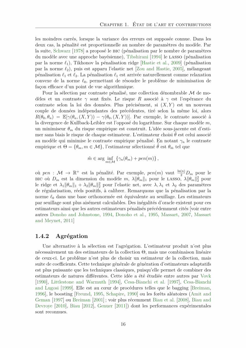
first one consists in representing the dimension of the selected model according toκ (Fig 2.3), and finding κ such that if κ < κ, the dimension of the selected modelis large, and reasonable otherwise. The slope heuristic prescribes then the use ofκ = 2κ. In the second one, one computes the asymptotic slope of the log-likelihooddrawn according to the model dimension, and penalizes the log-likelihood by twicethe slope times the model dimension. With our simulated data sets, we are in the notso common situation in which the jump is strong enough so that the first heuristiccan be used.
2.4.2 Simulated data sets
0 0.2 0.4 0.6 0.8 1−4
−2
0
2
4
6
8
10
X
Y
(a) 2 000 data points of example WS
0 0.2 0.4 0.6 0.8 1−4
−2
0
2
4
6
8
10
X
Y
(b) 2 000 data points of example MS
Figure 2.2 – Typical realizations
The previous procedure has been applied to two simulated data sets: one in whichtrue conditional density belongs to one of our models, a well-specified case, and onein which this is not true, a misspecified case. In the first situation, we expect toperform almost as well as the maximum likelihood estimation in the true model. Inthe second situation, we expect our algorithm to automatically balance the modelbias and its variance. More precisely, we let
s0(y|x) =1
1 + exp(15x− 7)Φ−15x+8,0.3(y) +
exp(15x− 7)1 + exp(15x− 7)
Φ0.4x+0.6,0.4(y)
in the first example, denoted example WS, and
s0(y|x) =1
1 + exp(15x− 7)Φ15x2−22x+7.4,0.3(y) +
exp(15x− 7)1 + exp(15x− 7)
Φ−0.4x2,0.4(y)
in the second example, denoted example MS. For both experiments, we let X beuniformly distributed over [0, 1]. Figure 2.2 shows a typical realization.
In both examples, we have noticed that the sample’s size had no significantinfluence on the choice of κ, and that very often 1 was in the range of possible valuesindicated by the jump criterion of the slope heuristic. According to this observation,we have chosen in both examples κ = 1.
35
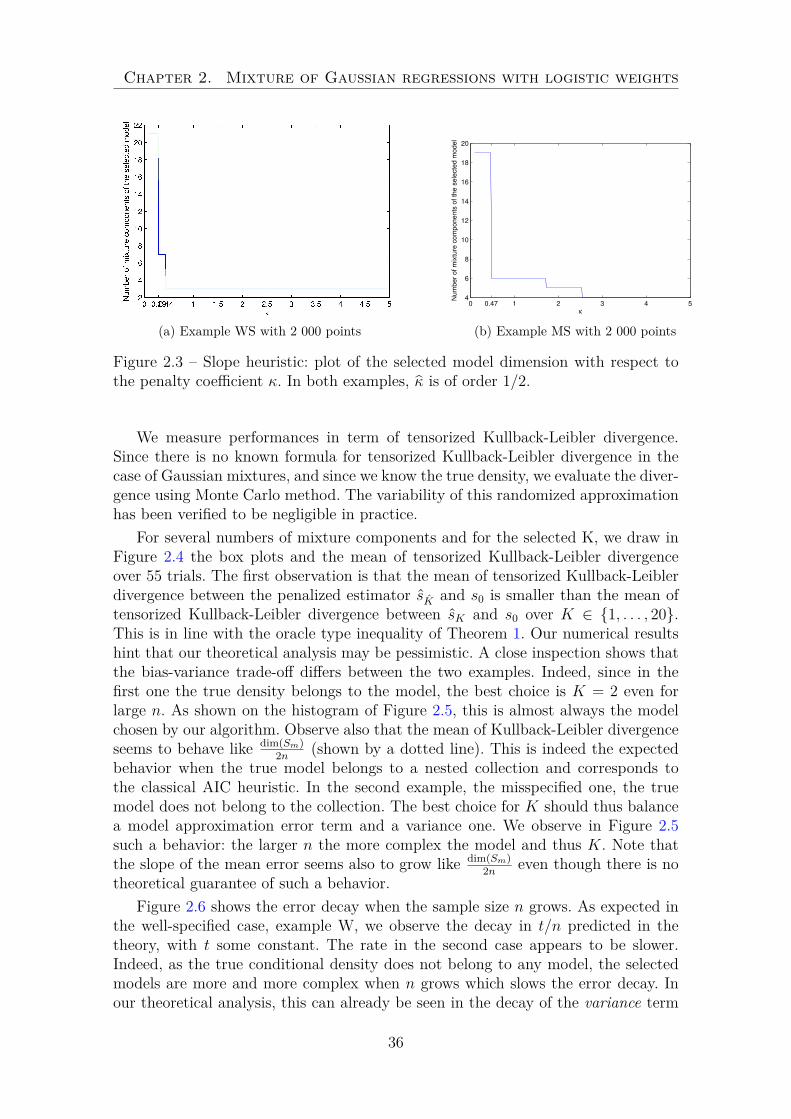
Chapter 2. Mixture of Gaussian regressions with logistic weights
(a) Example WS with 2 000 points
0 0.47 1 2 3 4 54
6
8
10
12
14
16
18
20
κ
Num
ber
of m
ixtu
re c
om
ponents
of th
e s
ele
cte
d m
odel
(b) Example MS with 2 000 points
Figure 2.3 – Slope heuristic: plot of the selected model dimension with respect tothe penalty coefficient κ. In both examples, κ is of order 1/2.
We measure performances in term of tensorized Kullback-Leibler divergence.Since there is no known formula for tensorized Kullback-Leibler divergence in thecase of Gaussian mixtures, and since we know the true density, we evaluate the diver-gence using Monte Carlo method. The variability of this randomized approximationhas been verified to be negligible in practice.
For several numbers of mixture components and for the selected K, we draw inFigure 2.4 the box plots and the mean of tensorized Kullback-Leibler divergenceover 55 trials. The first observation is that the mean of tensorized Kullback-Leiblerdivergence between the penalized estimator sK and s0 is smaller than the mean oftensorized Kullback-Leibler divergence between sK and s0 over K ∈ {1, . . . , 20}.This is in line with the oracle type inequality of Theorem 1. Our numerical resultshint that our theoretical analysis may be pessimistic. A close inspection shows thatthe bias-variance trade-off differs between the two examples. Indeed, since in thefirst one the true density belongs to the model, the best choice is K = 2 even forlarge n. As shown on the histogram of Figure 2.5, this is almost always the modelchosen by our algorithm. Observe also that the mean of Kullback-Leibler divergenceseems to behave like dim(Sm)
2n(shown by a dotted line). This is indeed the expected
behavior when the true model belongs to a nested collection and corresponds tothe classical AIC heuristic. In the second example, the misspecified one, the truemodel does not belong to the collection. The best choice for K should thus balancea model approximation error term and a variance one. We observe in Figure 2.5such a behavior: the larger n the more complex the model and thus K. Note thatthe slope of the mean error seems also to grow like dim(Sm)
2neven though there is no
theoretical guarantee of such a behavior.
Figure 2.6 shows the error decay when the sample size n grows. As expected inthe well-specified case, example W, we observe the decay in t/n predicted in thetheory, with t some constant. The rate in the second case appears to be slower.Indeed, as the true conditional density does not belong to any model, the selectedmodels are more and more complex when n grows which slows the error decay. Inour theoretical analysis, this can already be seen in the decay of the variance term
36

2.4. Numerical scheme and numerical experiment
1 2 3 4 5 6 7 8 9 10 11 12 13 14 15 16 17 18 19Selected K
0
0.005
0.01
0.015
0.02
0.025
0.03
0.035
0.04
0.045
0.05
asymptotic E[KL]
empirical E[KL]
E[KL] of the selected K
(a) Example WS with 2 000 data points
1 2 3 4 5 6 7 8 9 10 11 12 13 14 15 16 17 18 19 Selected K
0
2
4
6
8
10
12x 10
−3
asymptotic E[KL]
empirical E[KL]
E[KL] of the selected K
(b) Example WS with 10 000 data points
1 2 3 4 5 6 7 8 9 10 11 12 13 14 15 16 17 18 19Selected K
0.005
0.01
0.015
0.02
0.025
0.03
0.035
0.04
0.045
asymptotic E[KL]
empirical E[KL]
E[KL] of the selected K
(c) Example MS with 2 000 data points
1 2 3 4 5 6 7 8 9 10 11 12 13 14 15 16 17 18 19Selected K0
0.002
0.004
0.006
0.008
0.01
0.012
0.014
0.016
asymptotic E[KL]
empirical E[KL]
E[KL] of the selected K
(d) Example MS with 10 000 data points
Figure 2.4 – Box-plot of the Kullback-Leibler divergence according to the number ofmixture components. On each graph, the right-most box-plot shows this Kullback-Leibler divergence for the penalized estimator s
K
of the oracle inequality. Indeed, if we let m0(n) be the optimal oracle model, the oneminimizing the right-hand side of the oracle inequality, the variance term is of orderdim(Sm0(n))
nwhich is larger than 1
nas soon as dim(Sm0(n)) → +∞. It is well known
that the decay depends on the regularity of the true conditional density. Providing aminimax analysis of the proposed estimator, as have done Maugis and Michel [2012],would be interesting but is beyond the scope of this paper.
2.4.3 Ethanol data set
We explain now with more details the result of Figure 2.1 for the 88 data pointEthanol data set of Brinkman [1981]. Young [2014] proposes to estimate the densityof the equivalence ratio R conditioned to the concentration in NO and to use thisconditional density to do a clustering of the data set. In our framework, this amounts
37

Chapter 2. Mixture of Gaussian regressions with logistic weights
0 5 10 15 200
0.1
0.2
0.3
0.4
0.5
0.6
0.7
0.8
0.9
Selected number of classes
Em
piric
al p
rob
ab
ility
(a) Example WS with 2 000 data points
2 4 6 8 10 12 14 16 18 200
0.1
0.2
0.3
0.4
0.5
0.6
0.7
0.8
0.9
1
Selected number of classes
Em
piric
al p
rob
ab
ility
(b) Example WS with 10 000 data points
2 4 6 8 10 12 14 16 18 200
0.1
0.2
0.3
0.4
0.5
0.6
Selected number of classes
Em
piric
al p
rob
ab
ility
(c) Example MS with 2 000 data points
0 5 10 15 200
0.05
0.1
0.15
0.2
0.25
Selected number of classes
Em
pirirca
l p
rob
ab
ility
(d) Example MS with 10 000 data points
Figure 2.5 – Histograms of the selected K
to estimate the conditional density by
K∑
k=1
πwk(NO)Φυk(NO),Σk(R)
with our proposed penalized estimator and to use the classical maximum likelihoodapproach that associates (NO,R) to the class
arg max1≤k≤K
πwk(NO)Φυk(NO),Σk(R)
to perform the clustering.An important parameter of the method is the lower bound of the variance used
in the estimation for a given number of class. This is required to avoid spuriousmaximizers of the likelihood. Here, the value 10−4 chosen by hand yields satisfactoryresults.
Since we only have 88 points and roughly 5 parameters per class, the randominitialization may yield classes with too few points to have a good estimation. Wehave slightly modified our K-means procedure in order to ensure than at least 10
38

2.4. Numerical scheme and numerical experiment
103
104
10−4
10−3
10−2
Sample’s size
me
an
of
Ku
llba
ck−
Le
ible
r d
ista
nce
ove
r 3
0 t
ria
ls
E[KL]
n−>t/n
linear regression of E[KL]
(a) Example WS. The slope of the free regressionline is ≃ −1, 3
103
104
10−2
Sample’s size
Te
nso
rize
d K
ullb
ack−
Le
ible
r d
ista
nce
E[KL]
n−>t/n
linear regression of E[KL]
(b) Example MS. The slope of the regression line is≃ −0, 6.
Figure 2.6 – Kullback-Leibler divergence between the true density and the computeddensity using (Xi, Yi)i≤N with respect to the sample size, represented in a log-logscale. For each graph, we added a free linear least-square regression and one withslope −1 to stress the two different behavior.
points are assigned to each class. In that case, we have verified that the estimatedparameters of the conditional density were very stable.
Note that with this strategy, no more than 8 classes can be considered. Thisprevents the use of the jump criterion to calibrate the penalty because the big jumpis hard to define. We use instead the slope heuristic. Figure 2.7 shows that thisslope is of order 1 and thus the slope heuristic prescribes a penalty of 2 dim(SK),providing an estimate with 4 components.
It is worth pointing out that the maximum of the penalized likelihood is notsharp, just like in the example MS of simulated data (see figure 2.5). Indeed, itis quite unlikely that the true density belongs to our model collection. So, theremay be an uncertainty on the selected number of components between 4, 3 and 5.Note that AIC penalization would have lead to 7 classes while BIC would also havelead to 4 classes. Our estimated penalty is nevertheless in the middle of the zonecorresponding to 4 while BIC is nearby the boundary with 3 and thus we expectthis choice to be more stable. In Figure 2.1b of the introduction we have shown onlythis clustering with 4 classes. Figure 2.8 shows that the choices of 3 or 5 may makesense, even though the choice 5 may seem slightly too complex. A common featureamong all those clusterings is the change of slope in the topmost part around 1.7.This phenomena is also visible in Young [2014] in which an explicit change pointmodel is used, ours is only implicit and thus more versatile
To complete our study, in Figure 2.9, we have considered the more natural regres-sion of NO with respect to the equivalence ratio that has not been studied by Young[2014]. Using the same methodology, we have recovered also 4 clusters correspond-ing to a soft partitioning of the equivalence ratio value. Note that this clustering,which is easily interpretable, is very similar to the one obtained with the previousparameterization.
39

Chapter 2. Mixture of Gaussian regressions with logistic weights
0 0,703 1,282 1,737 2,261 2,522 32
3
4
5
6
7
8
κ
Num
ber
of m
ixtu
re c
om
ponents
of th
e s
ele
cte
d m
odel
(a) Jump criterion
0 5 10 15 20 25 30 35 400
20
40
60
80
100
120
140
160
180
Model dimension
Lo
g−
like
liho
od
Log−likelihood
Asymptotic slope
Penalized log−likelihood
(b) Slope criterion
Figure 2.7 – Slope heuristic for the ethanol data set
2.4.4 ChIP-chip data set
We consider here a second real data set: a Chromatin immunoprecipitation(ChIP) on chip genomic data set. Chromatin immunoprecipitation (ChIP) is a pro-cedure used to investigate proteins associated with DNA. The data set considered isthe one used by Martin-Magniette et al. [2008]. In this experiment, two variables arestudied: DNA fragments crosslinked to a protein of interest (IP) and genomic DNA(Input). Martin-Magniette et al. [2008] model the density of log-IP conditioned tolog-Input by a mixture of two Gaussian regressions with the same variance. Onecomponent corresponds to an enriched one, in which there is more proteins thanexpected, and the other to a normal one. They use classical proportions that donot depend on the Input. The parameters are estimated using the EM algorithminitialized by values derived from a Principal Component Analysis of the whole dataset. The best model between one and two components is selected according to theBIC criterion. For the histone modification in Arabidopsis thaliana data set, theyselect a two components model similar to the one obtained with logistic weights(Figure 2.10).
We have first compared the constant proportions model with K = 2 to the oneproposed in their conclusion in which the proportions depend on the Input. We haveused our affine logistic weights model and observed that this model greatly improvesthe log-likelihood. The dimension of this new model is 8 while the dimension of theoriginal model is 7 so that the log-likelihood increase does not seem to be due tooverfitting. We have also compared our solution to the one obtained with a constantweights model with K = 3, of dimension 11. The BIC criterion selects the K = 2with affine weights solution.
We have then tested more complex models with K up to 20 with a penaltyobtained with the slope heuristic. The models chosen are quite complex (K = 10for constant proportions models and K = 7 for affine logistic weight models, thelater being the overall winner). Although they better explain the data from thestatistical point of view, those models become hard to interpret from the biologicalpoint of view. We think this is due to the too simple affine models used. Although
40

2.5. Discussion
0 0.5 1 1.5 2 2.5 3 3.5 4 4.50.5
0.6
0.7
0.8
0.9
1
1.1
1.2
1.3
NO
Equiv
ale
nce R
atio
(a) K=2
0 0.5 1 1.5 2 2.5 3 3.5 4 4.50.5
0.6
0.7
0.8
0.9
1
1.1
1.2
1.3
NO
Equiv
ale
nce R
atio
(b) K=3
0 0.5 1 1.5 2 2.5 3 3.5 4 4.50.4
0.5
0.6
0.7
0.8
0.9
1
1.1
1.2
1.3
NO
Equ
ival
ence
Rat
io
(c) K=4
0 0.5 1 1.5 2 2.5 3 3.5 4 4.50.5
0.6
0.7
0.8
0.9
1
1.1
1.2
1.3
NO
Equiv
ale
nce R
atio
(d) K=5
Figure 2.8 – Clustering of NO data set into K classes. The strength of the color ofthe regression lines corresponds to the mixture proportion.
no conceptual difficulties occur by using more complex function familie (or goingto the multivariate setting), the curse of dimensionality makes everything morecomplicated in practice. In particular, initialization becomes harder and harder asthe dimension grows and requires probably a more clever treatment than the oneproposed here. In the spirit of Cohen and Le Pennec [2013], we are currently workingon a first extension: a numerical algorithm for a bivariate piecewise linear logisticweights model applied to hyperspectral image segmentation.
2.5 Discussion
We have studied a penalized maximum likelihood estimate for mixtures of Gaus-sian regressions with logistic weights. Our main contribution is the proof that apenalty proportional, up to a logarithmic factor of the sample size, to the dimensionof the model is sufficient to obtain a non asymptotic theoretical control on the esti-mator loss. This result is illustrated in the simple univariate case in which both themeans and the logistic weights are linear. We study a toy model which exhibits the
41

Chapter 2. Mixture of Gaussian regressions with logistic weights
0.5 0.6 0.7 0.8 0.9 1 1.1 1.2 1.30
0.5
1
1.5
2
2.5
3
3.5
4
4.5
Equivalence Ratio
NO
Figure 2.9 – Clustering of NO data set into 4 classes, considering the regression ofNO with respect to the equivalence ratio
behavior predicted by our theoretical analysis and proposes two simple applicationsof our methodology. We hope that our contribution helps to popularize those mix-tures of Gaussian regressions by giving a theoretical foundation for model selectiontechnique in this area and showing some possible interesting uses even for simplemodels.
Besides some important theoretical issues on the loss used and the tightness ofthe bounds, the major future challenge is the extension of the numerical scheme tomore complex cases than univariate linear models.
2.6 Appendix : A general conditional density modelselection theorem
We summarize in this section the main result of Cohen and Le Pennec [2011]that will be our main tool to obtain the previous oracle inequality.
To any model Sm, a set of conditional densities, we associate a complexity definedin term of a specific entropy, the bracketing entropy with respect to the square root ofthe tensorized square of the Hellinger distance d2⊗n. Recall that a bracket [t−, t+] is apair of real functions such that ∀(x, y) ∈ X ×Y , t−(x, y) ≤ t+(x, y) and a function s issaid to belong to the bracket [t−, t+] if ∀(x, y) ∈ X ×Y , t−(x, y) ≤ s(x, y) ≤ t+(x, y).The bracketing entropy H[],d(δ, S) of a set S is defined as the logarithm of theminimal number N[],d(δ, S) of brackets [t−, t+] covering S, such that d(t−, t+) ≤ δ.The main assumption on models is a property that should satisfies the bracketingentropy:
Assumption (H) For every model Sm in the collection S, there is a non-decreasing function φm such that δ 7→ 1
δφm(δ) is non-increasing on (0,+∞)
and for every σ ∈ R+,∫ σ
0
√H[.],d⊗n(δ, Sm)dδ ≤ φm(σ).
Such an integral is ofter called a Dudley type integral of these bracketing entropiesand is commonly used in empirical process theory [van der Vaart and Wellner, 1996].
42

2.6. Appendix : A general conditional density model selectiontheorem
(a) K=2, constant proportions,dimension= 7
(b) K=2, affine logistic weights,dimension= 8
(c) K=3, constant proportions,dimension= 9
(d) K=7, affine logistic weights,dimension= 33
(e) K=10, constant propor-tions, dimension= 39
Figure 2.10 – Clustering of ChIP-chip data set into K classes.
The complexity of Sm is then defined as nσ2m where σm is the unique square root of
1σφm(σ) =
√nσ.
For technical reason, a separability assumption, always satisfied in the settingof this paper, is also required. It is a mild condition, classical in empirical processtheory (see for instance van der Vaart and Wellner [1996]).
Assumption (Sep) For every model Sm in the collection S, there exists somecountable subset S ′
m of Sm and a set Y ′m with λ(Y\Y ′
m) = 0 such that forevery t in Sm, there exists some sequence (tk)k≥1 of elements of S ′
m such thatfor every x ∈ X and every y ∈ Y ′
m, ln(tk(y|x)) −−−−→k→+∞
ln(t(y|x)).
The main result of Cohen and Le Pennec [2011] is a condition on the penaltypen(m) which ensures an oracle type inequality:
Theorem 2. Assume we observe (Xi, Yi) with unknown conditional density s0. LetS = (Sm)m∈M an at most countable conditional density model collection. AssumeAssumptions (H), (Sep) and (K) hold. Let sm be a η minimizer of the negativelog-likelihood in Sm
n∑
i=1
− ln(sm(Yi|Xi)) ≤ infsm∈Sm
(n∑
i=1
− ln(sm(Yi|Xi))
)+ η
Then for any ρ ∈ (0, 1) and any C1 > 1, there is a constant κ0 depending onlyon ρ and C1 such that, as soon as for every index m ∈ M,
pen(m) ≥ κ(nσ2m + xm)
43

Chapter 2. Mixture of Gaussian regressions with logistic weights
with κ > κ0 and σm the unique square root of 1σφm(σ) =
√nσ, the penalized likelihood
estimate sm with m such that
n∑
i=1
− ln(sm(Yi|Xi)) + pen(m) ≤ infm∈M
(n∑
i=1
− ln(sm(Yi|Xi)) + pen(m)
)+ η′
satisfies
E[JKL⊗n
ρ (s0, sm)]
≤ C1 infm∈M
(inf
sm∈Sm
KL⊗n(s0, sm) +pen(m)
n
)+ C1
κ0Ξ + η + η′
n.
In the next section, we show how to apply this result in our mixture of Gaussianregressions setting and prove that the penalty can be chosen roughly proportionalto the intrinsic dimension of the model, and thus of the order of the variance.
2.7 Appendix : Proofs
In Appendix 2.7.1, we give a proof of Theorem 1 relying on several bracketingentropy controls proved in Appendix 2.7.2.
2.7.1 Proof of Theorem 1
We will show that Assumption (DIM) ensures that for all δ ∈ (0,√
2], H[.],d⊗n(δ, Sm) ≤dim(Sm)(C + ln(1
δ)) with a common C.
We show in Appendix that ifAssumption (DIM) There exist two constants CW and CΥ such that, for every
model Sm in the collection S,
Hd‖ sup ‖∞(σ,WK) ≤ dim(WK)
(CW + ln
1σ
)
andHd‖ sup ‖∞
(σ,ΥK) ≤ dim(ΥK)(CΥ + ln
1σ
)
then, if n ≥ 1, the complexity of the corresponding model Sm satisfies for anyδ ∈ (0,
√2],
H[.],d⊗n(δ, Sm) ≤ dim(Sm)(C + ln(1δ
))
with dim(Sm) = dim(WK) + dim(ΥK) + dim(VK) and C that depends only on theconstants defining VK and the constants CW and CΥ.
If this happens, Proposition 1 yields the results.
Proposition 1. If for any δ ∈ (0,√
2], H[.],d⊗n(δ, Sm) ≤ dim(Sm)(Cm + ln(1δ)), then
the function φm(σ) = σ√
dim(Sm)(√
Cm +√π +
√ln(
1min(σ,1)
))satisfies Assump-
tion (H). Furthermore, the unique square root σm of 1σφm(σ) =
√nσ satisfies
nσ2m ≤ dim(Sm)
(2(√Cm +
√π)2 +
(ln
n
(√Cm +
√π)2 dim(Sm)
)
+
).
44

2.7. Appendix : Proofs
In other words, if we can control models’ bracketing entropy with a uniform con-stant C, we get a suitable bound on the complexity. This result will be obtain by firstdecomposing the entropy term between the weights and the Gaussian components.Therefore we use the following distance over conditional densities:
supxdy(s, t) = sup
x∈X
(∫
y
(√s(y|x) −
√t(y|x)
)2
dy
) 12
.
Notice that d2⊗n(s, t) ≤ supx d2y(s, t).
For all weights π and π′, we define
supxdk(π, π′) = sup
x∈X
(K∑
k=1
(√πk(x) −
√π′
k(x))2) 1
2
.
Finally, for all densities s and t over Y , depending on x, we set
supx
maxk
dy(s, t) = supx∈X
max1≤k≤K
dy(sk(x, .), tk(x, .))
= supx∈X
max1≤k≤K
(∫
y
(√sk(x, y) −
√tk(x, y)
)2
dy
) 12
.
Lemma 3. Let P ={
(πw,k)1≤k≤K
∣∣∣w ∈ WK , and ∀(k, x), πw,k(x) = ewk(x)∑K
l=1ewl(x)
}and
G ={(Φυk,Σk
)1≤k≤K |υ ∈ ΥK ,Σ ∈ VK
}. Then for all δ in (0,
√2], for all m in M,
H[.],supx
dy (δ, Sm) ≤ H[.],supx
dk
(δ
5,P)
+H[.],supx
maxk
dy
(δ
5,G).
One can then relate the bracketing entropy of P to the entropy of WK
Lemma 4. For all δ ∈ (0,√
2],
H[.],supx
dk
(δ
5,P)
≤ Hd‖ sup ‖∞
(3√
3δ
20√K,WK
)
Since P is a set of weights, 3√
3δ20
√K
could be replaced by 3√
3δ20
√K−1
with an identi-fiability condition. For example, W ′
K = {(0, w2 − w1, . . . , wK − w1)|w ∈ WK} canbe covered using brackets of null size on the first coordinate, lowering squaredHellinger distance between the brackets’ bounds to a sum of K−1 terms. Therefore,H[.],sup
x
dk
(δ5,P)
≤ Hd‖ sup ‖∞
(3√
3δ20
√K−1
,W ′K
).
Since we have assumed that ∃CW s.t ∀δ ∈ (0,√
2],
Hd‖ sup ‖∞(δ,WK) ≤ dim(WK)
(CW + ln
(1δ
))
Then
H[.],supx
dk
(δ
5,P)
≤ dim(WK)
(CW + ln
(20
√K
3√
3δ
))
To tackle the Gaussian regression part, we rely heavily on the following propo-sition,
45

Chapter 2. Mixture of Gaussian regressions with logistic weights
Proposition 2. Let κ ≥ 1729
, γκ =25(κ− 1
2)
49(1 + 2κ5
). For any 0 < δ ≤
√2 and any δΣ ≤
1
5√
κ2 cosh( 2κ5
)+ 12
δp, (υ, L,A, P ) ∈ Υ× [L−, L+]×A(λ−, λ+)×SO(p) and (υ, L, A, P ) ∈
Υ × [L−, L+] × A(λ−,+∞) × SO(p),Σ = LPAP ′ and Σ = LP AP ′, assume thatt−(x, y) = (1 + κδΣ)−pΦυ(x),(1+δΣ)−1Σ(y) and t+(x, y) = (1 + κδΣ)pΦυ(x),(1+δΣ)Σ(y).
If
∀x ∈ Rd, ‖υ(x) − υ(x)‖2 ≤ pγκL−λ−λ−
λ+δΣ
2
(1 + 225δΣ)−1L ≤ L ≤ L
∀1 ≤ i ≤ p, |A−1i,i − A−1
i,i | ≤ 110
δΣ
λ+
∀y ∈ Rp, ‖Py − P y‖ ≤ 110
λ−
λ+δΣ‖y‖
then [t−, t+] is a δ5
Hellinger bracket such that t−(x, y) ≤ Φυ(x),Σ(y) ≤ t+(x, y).
We consider three cases: the parameter (mean, volume, matrix) is known (⋆ = 0),unknown but common to all classes (⋆ = c), unknown and possibly different for everyclass (⋆ = K). For example, [νK , L0, Pc, A0] denotes a model in which only meansare free and eigenvector matrices are assumed to be equal and unknown. Under ourassumption that ∃CΥ s.t ∀δ ∈ (0,
√2],
Hd‖ sup ‖∞(δ,ΥK) ≤ dim(ΥK)
(CΥ + ln
(1δ
))
we deduce:
H[.],maxk supx dy
(δ
5,G)
≤ D(
C + ln(1δ
))(2.1)
where D = Zυ,⋆ + ZL,⋆ +p(p− 1)
2ZP,⋆ + (p− 1)ZA,⋆ and
C = ln
5p
√κ2 cosh
(2κ5
)+
12
+
Zυ,⋆CΥ
D +Zυ,⋆
2D ln
(λ+
pγκL−λ2−
)
+ZL,⋆
D ln
4 + 129 ln(
L+
L−
)
10
+
ZP,⋆
D
(ln(cU) +
p(p− 1)2
ln
(10λ+
λ−
))
+ZA,⋆(p− 1)
D ln
(45
+52λ+
5λ−ln
(λ+
λ−
))
Zυ,K = dim(ΥK), Zυ,c = dim(Υ1), Zυ,0 = 0 ZL,0 = ZP,0 = ZA,0 = 0,
ZL,c = ZP,c = ZA,c = 1, ZL,K = ZP,K = ZA,K = K.
We notice that the following upper-bound of C is independent from the model
46
2.7. Appendix : Proofs
of the collection, because we have made this hypothesis on CΥ.
C ≤ ln
5p
√κ2 cosh
(2κ5
)+
12
+ CΥ +
12
ln
(λ+
pγκL−λ2−
)
+ ln
4 + 129 ln(
L+
L−
)
10
+
2p(p− 1)
ln(cU) + ln
(10λ+
λ−
)
+ ln
(45
+52λ+
5λ−ln
(λ+
λ−
)):= C1.
We conclude that H[.],supx dy (δ, Sm) ≤ dim(Sm)(Cm + ln
(1δ
)), with
dim(Sm) = dim(WK) + D
Cm =dim(WK)dim(Sm)
(CW + ln
(20
√K
3√
3
))+
DC1
dim(Sm)
≤ CW + ln
(20
√Kmax
3√
3
)+ C1 := C
Note that the constant C does not depend on the dimension dim(Sm) of the model,thanks to the hypothesis that CW is common for every model Sm in the collection.Using Proposition 1, we deduce thus that
nσ2m ≤ dim(Sm)
2
(√C +
√π)2
+
ln
n(√
C +√π)2
dim(Sm)
+
.
Theorem 2 yields then, for a collection S = (Sm)m∈M, with M = {(K,WK ,ΥK , VK)|K ∈N\{0},WK ,ΥK , VK as previously defined } for which Assumption (K) holds, the or-acle inequality of Theorem 1 as soon as
pen(m) ≥ κ
dim(Sm)
2
(√C +
√π)2
+
ln
n(√
C +√π)2
dim(Sm)
+
+ xm
.
2.7.2 Lemma Proofs
Bracketing entropy’s decomposition
We prove here a slightly more general Lemma than Lemma 3.
Lemma 5. Let
P =
{π = (πk)1≤k≤K
∣∣∣∀k, πk : X → R+ and ∀x ∈ X ,K∑
k=1
πk(x) = 1
},
Ψ ={
(ψ1, . . . , ψK)∣∣∣∀k, ψk : X × Y → R+, and ∀x, ∀k,
∫ψk(x, y)dy = 1
},
C =
{(x, y) 7→
K∑
k=1
πk(x)ψk(x, y)∣∣∣π ∈ P, ψ ∈ Ψ
}.
47

Chapter 2. Mixture of Gaussian regressions with logistic weights
Then for all δ in (0,√
2],
H[.],supx
dy (δ, C) ≤ H[.],supx
dk
(δ
5,P)
+H[.],supx
maxk
dy
(δ
5,Ψ
).
The proof mimics the one of Lemma 7 from Cohen and Le Pennec [2011]. It ispossible to obtain such an inequality if the covariate X is not bounded, using thesmaller distance d⊗n for the entropy with bracketing of C. More precisely,
Lemma 6. For all δ in (0,√
2], H[.],d⊗n (δ, C) ≤ H[.],dP
(δ2,P)
+H[.],dΨ
(δ2,Ψ),
with d2P(π+, π−) = E
[1n
n∑
i=1
d2k(π+(Xi), π−(Xi))
]and
d2Ψ(ψ+, ψ−) = E
[1n
n∑
i=1
K∑
k=1
d2y(ψ+
k (Xi), ψ−k (Xi))
]. But bounding such bracketing en-
tropies for P and Ψ becomes much more challenging.
Proof. First we will exhibit a covering of bracket of C.Let ([πi,−, πi,+])1≤i≤NP
be a minimal covering of δ bracket for supx dk of P :
∀i ∈ {1, . . . , NP},∀x ∈ X , dk(πi,−(x), πi,+(x)) ≤ δ.
Let ([ψi,−, ψi,+])1≤i≤NΨbe a minimal covering of δ bracket for sup
xmax
kdy of Ψ:
∀i ∈ {1, . . . , NΨ},∀x ∈ X ,∀k ∈ {1, . . . , K}, dy(ψi,−k (x, .), ψi,+
k (x, .)) ≤ δ.
Let s be a density in C. By definition, there is π in P and ψ in Ψ such that for all(x, y) in X × Y , s(y|x) =
∑Kk=1 πk(x)ψk(x, y).
Due to the covering, there is i in {1, . . . , NP} such that
∀x ∈ X ,∀k ∈ {1, . . . , K}, πi,−k (x) ≤ πk(x) ≤ πi,+
k (x).
There is also j in {1, . . . , NΨ} such that
∀x ∈ X ,∀k ∈ {1, . . . , K},∀y ∈ Y , ψj,−k (x, y) ≤ ψk(x, y) ≤ ψj,+
k (x, y).
Since for all x, for all k and for all y, πk(x) and ψk(x, y) are non-negatives, wemay multiply term-by-term and sum these inequalities over k to obtain:
∀x ∈ X ,∀y ∈ Y ,K∑
k=1
(πi,−
k (x))
+
(ψj,−
k (x, y))
+≤ s(y|x) ≤
K∑
k=1
πi,+k (x)ψj,+
k (x, y).
([K∑
k=1
(πi,−
k
)+
(ψj,−
k
)+,
K∑
k=1
πi,+k ψj,+
k
])
1≤i≤NP1≤j≤NΨ
is thus a bracket covering of C.
Now, we focus on brackets’ size using lemmas from Cohen and Le Pennec [2011](namely Lemma 11, 12, 13), To lighten the notations, π−
k and ψ−k are supposed non-
negatives for all k. Following their Lemma 12, only using Cauchy-Schwarz inequality,we prove that
supxd2
y
(K∑
k=1
π−k (x)ψ−
k (x, .),K∑
k=1
π+k (x)ψ+
k (x, .)
)
≤ supxd2
y,k(π−(x)ψ−(x, .), π+(x)ψ+(x, .)).
48

2.7. Appendix : Proofs
Then, using Cauchy-Schwarz inequality again, we get by their Lemma 11:
supxd2
y,k(π−(x)ψ−(x, .), π+(x)ψ+(x, .))
≤ supx
max
kdy(ψ+
k (x, .), ψ−k (x, .))
√√√√K∑
k=1
π+k (x)
+dk(π+(x), π−(x)) maxk
√∫ψ−
k (x, y)dy
)2
According to their Lemma 13, ∀x,∑Kk=1 π
+k (x) ≤ 1 + 2(
√2 +
√3)δ.
supx
max
kdy(ψ+
k (x, .), ψ−k (x, .))
√√√√K∑
k=1
π+k (x)
+dk(π+(x), π−(x)) maxk
√∫ψ−
k (x, y)dy
)2
≤(√
1 + 2(√
2 +√
3)δ + 1)2
δ2 ≤ (5δ)2
The result follows from the fact we exhibited a 5δ covering of brackets of C, withcardinality NPNΨ.
Bracketing entropy of weight’s families
General case We prove
Lemma 4. For any δ ∈ (0,√
2],
H[.],supx dk
(δ
5,P)
≤ Hd‖ sup ‖∞
(3√
3δ
20√K,WK
).
Proof. We show that ∀(w, z) ∈ (WK)2,∀k ∈ {1, . . . , K},∀x ∈ X , |√πw,k(x) −√
πz,k(x)| ≤ F (k, x)d(w, z), with F a function and d some distance. We define
∀k,∀u ∈ RK , Ak(u) = exp(uk)∑K
k=1exp(uk)
, so πw,k(x) = Ak(w(x)).
∀(u, v) ∈ (RK)2,
∣∣∣∣√Ak(v) −
√Ak(u)
∣∣∣∣ =∣∣∣∣∫ 1
0∇(√
Ak
)(u+ t(v − u)).(v − u)dt
∣∣∣∣
Besides,
∇(√
Ak
)(u) =
(12
√Ak(u)
∂
∂ul
(ln(Ak(u)))
)
1≤l≤K
=(1
2
√Ak(u) (δk,l − Al(u))
)
1≤l≤K
49

Chapter 2. Mixture of Gaussian regressions with logistic weights
∣∣∣∣√Ak(v) −
√Ak(u)
∣∣∣∣
=12
∣∣∣∣∣
∫ 1
0
√Ak(u+ t(v − u))
K∑
l=1
(δk,l − Al(u+ t(v − u))) (vl − ul)dt
∣∣∣∣∣
≤ ‖v − u‖∞2
∫ 1
0
√Ak(u+ t(v − u))
K∑
l=1
|δk,l − Al(u+ t(v − u))| dt
Since ∀u ∈ RK ,∑K
k=1 Ak(u) = 1,∑K
l=1 |δk,l − Al(u)| = 2(1 − Ak(u))
∣∣∣∣√Ak(v) −
√Ak(u)
∣∣∣∣ ≤ ‖v − u‖∞
∫ 1
0
√Ak(u+ t(v − u)) (1 − Ak(u+ t(v − u))) dt
≤ 23√
3‖v − u‖∞
since x 7→ √x(1 − x) is maximal over [0,1] for x = 1
3. We deduce that for any
(w, z) in (WK)2, for all k in {1, . . . , K}, for any x in X , |√πw,k(x) −
√πz,k(x)| ≤
23√
3maxl ‖wl − zl‖∞.By hypothesis, for any positive ǫ, an ǫ-net N ofWK may be exhibited. Let w be an
element of WK . There is a z belonging to the ǫ-net N such that maxl ‖zl −wl‖∞ ≤ ǫ.Since for all k in {1, . . . , K}, for any x in X ,
|√πw,k(x) −
√πz,k(x)| ≤ 2
3√
3max
l‖wl − zl‖∞ ≤ 2
3√
3ǫ,
andK∑
k=1
(√πz,k(x) +
23√
3ǫ−
√πz,k(x) +
23√
3ǫ
)2
= K
(4ǫ
3√
3
)2
,
([(√πz − 2
3√
3ǫ)2,(√
πz + 23√
3ǫ)2])
z∈Nis a 4ǫ
√K
3√
3-bracketing cover of P . As a result,
H[],supx dk
(δ5,P)
≤ Hd‖ sup ‖∞
(3√
320
√Kδ,WK
).
Case: WK = {0} ⊗WK−1 with W constructed from bounded functions Weremind that
W =
w : X → R/w(x) =
dW∑
i=0
αiψW,i and ‖α‖∞ ≤ TW
with ‖ψW,i‖∞ ≤ 1.
Proof of Part 1 of Lemma 1. WK is a finite dimensional compact set. Thanks to theresult in the general case, we get
H[.],supx
dk
(δ
5,P)
≤ Hd‖ sup ‖∞
(3√
3δ20
√K − 1
,WK
)
50

2.7. Appendix : Proofs
now as for all w, v inWK , maxk ‖wk−vk‖∞ ≤ maxk∑dW
i=0 |αwk,i−αv
k,i| ≤ dW maxk,i |αwk,i−
αvk,i|
≤ H‖.‖∞
(3√
3δ20
√K − 1dW
,{α ∈ R(K−1)dW /‖α‖∞ ≤ TW
})
≤ (K − 1)dW ln
(1 +
20√K − 1TWdW
3√
3δ
)
≤ (K − 1)dW
[ln
(√2 +
203√
3TW
√K − 1dW
)+ ln
(1δ
)]
The second Lemma is just a consequence of dW =(
d′W +d
d
)
Bracketing entropy of Gaussian families
General case We rely on a general construction of Gaussian brackets:
Proposition. 2. Let κ ≥ 1729
, γκ =25(κ− 1
2)
49(1 + 2κ5
). For any 0 < δ ≤
√2, any p ≥ 1
and any δΣ ≤ 1
5√
κ2 cosh( 2κ5
)+ 12
δp, let (υ, L,A, P ) ∈ Υ × [L−, L+] × A(λ−, λ+) × SO(p)
and (υ, L, A, P ) ∈ Υ × [L−, L+] × A(λ−,+∞) × SO(p), define Σ = LPAP ′ andΣ = LP AP ′,
t−(x, y) = (1 + κδΣ)−pΦυ(x),(1+δΣ)−1Σ(y) and t+(x, y) = (1 + κδΣ)pΦυ(x),(1+δΣ)Σ(y).
If
∀x ∈ X , ‖υ(x) − υ(x)‖2 ≤ pγκL−λ−λ−
λ+δ2
Σ(1 + 2
25δΣ
)−1L ≤ L ≤ L
∀1 ≤ i ≤ p, |A−1i,i − A−1
i,i | ≤ 110
δΣ
λ+
∀y ∈ Rp, ‖Py − P y‖ ≤ 110
λ−
λ+δΣ‖y‖
then [t−, t+] is a δ/5 Hellinger bracket such that t−(x, y) ≤ Φυ(x),Σ(y) ≤ t+(x, y).
This statement is similar to Lemma 10 in Cohen and Le Pennec [2011]. Admit-ting this proposition, we are brought to construct nets over the spaces of the means,the volumes, the eigenvector matrices and the normalized eigenvalue matrices. Weconsider three cases: the parameter (mean, volume, matrix) is known (⋆ = 0), un-known but common to all classes (⋆ = c), unknown and possibly different for everyclass (⋆ = K). For example, [νK , L0, Pc, A0] denotes a model in which only meansare free and eigenvector matrices are assumed to be equal and unknown.
51

Chapter 2. Mixture of Gaussian regressions with logistic weights
If the means are free (⋆ = K), we construct a grid GΥKover ΥK , which is
compact. Since
Hd‖ sup ‖∞
(√pγκL−λ−
λ−λ+
δΣ,ΥK
)≤ dim(ΥK)
CΥ + ln
1√pγκL−λ−
λ−
λ+δΣ
,
∣∣∣∣∣GΥK
(√pγκL−λ−
λ−λ+
δΣ
)∣∣∣∣∣ ≤
CΥ + ln
1√pγκL−λ−
λ−
λ+δΣ
dim(ΥK)
.
If the means are common and unknown (⋆ = c), belonging to Υ1 , we construct a
grid GΥc
(√pγκL−λ−
λ−
λ+δΣ
)over Υ1 with cardinality at most
CΥ + ln
1√pγκL−λ−
λ−
λ+δΣ
DΥ1
.
Finally, if the means are known (⋆ = 0), we do not need to construct a grid. In
the end,∣∣∣∣GΥ⋆
(√pγκL−λ−
λ−
λ+δΣ
)∣∣∣∣ ≤CΥ + ln
1√
pγκL−λ−λ−λ+
δΣ
Zυ,⋆
, with Zυ,K =
dim(ΥK), Zυ,c = DΥ1 and Zυ,0 = 0.Then, we consider the grid GL over [L−, L+]:
GL
( 225δΣ
)={L−
(1 +
225δΣ
)g
/g ∈ N, L−
(1 +
225δΣ
)g
≤ L+
}
∣∣∣∣GL
( 225δΣ
)∣∣∣∣ ≤ 1 +ln(
L+
L−
)
ln(1 + 2
25δΣ
)
Since δΣ ≤ 25, ln
(1 + 2
25δΣ
)≥ 10
129δΣ.
∣∣∣∣GL
( 225δΣ
)∣∣∣∣ ≤ 1 +129 ln
(L+
L−
)
10δΣ
≤4 + 129 ln
(L+
L−
)
10δΣ
By definition of a net, for any P ∈ SO(p) there is a P ∈ GP
(110
λ−
λ+δΣ
)such that
∀y ∈ Rp, ‖Py − P y‖ ≤ 110
λ−
λ+δΣ‖y‖. There exists a universal constant cU such that
∣∣∣GP
(110
λ−
λ+δΣ
)∣∣∣ ≤ cU
(10λ+
λ−δΣ
) p(p−1)2 .
For the grid GA, we look at the condition on the p− 1 first diagonal values andobtain: ∣∣∣∣∣GA
(110λ−λ+
δΣ
)∣∣∣∣∣ ≤2 +
ln(
λ+
λ−
)
ln(1 + 1
10λ−
λ+δΣ
)
p−1
Since δΣ ≤ 25, ln
(1 + 1
10λ−
λ+δΣ
)≥ 5
52λ−
λ+δΣ, then
∣∣∣∣∣GA
(110λ−λ+
δΣ
)∣∣∣∣∣ ≤(
2 +525δΣ
λ+
λ−ln
(λ+
λ−
))p−1
≤(
4 + 52λ+
λ−ln
(λ+
λ−
))p−1 ( 15δΣ
)p−1
52

2.7. Appendix : Proofs
Let ZL,0 = ZP,0 = ZA,0 = 0, ZL,c = ZP,c = ZA,c = 1, ZL,K = ZP,K = ZA,K =
K. We define fυ,⋆ from Υ⋆ to ΥK by
0 7→ (υ0,1, . . . , υ0,1) if ⋆ = 0
υ 7→ (υ, . . . , υ) if ⋆ = c
(υ1, . . . , υK) 7→ (υ1, . . . , υK) if ⋆ = K
and
similarly fL,⋆, fP,⋆ and fA,⋆, respectively from (R+)ZL,⋆ into (R+)K , from (SO(p))ZP,⋆
into (SO(p))K and from A(λ−, λ+)ZA,⋆ into A(λ−, λ+)K .We define
Γ : (υ1, . . . , υK , L1, . . . , LK , P1, . . . , PK , A1, . . . , AK) 7→ (υk, LkPkAkP′k)1≤k≤K
and Ψ : (υk,Σk)1≤k≤K 7→ (Φυk,Σk)1≤k≤K . The image of Υ⋆×[L−, L+]ZL,⋆×SO(p)ZP,⋆×
A(λ−, λ+)ZA,⋆ by Ψ◦Γ◦(fυ,⋆⊗fL,⋆⊗fP,⋆⊗fA,⋆) is the set G of all K-tuples of Gaussiandensities of type [υ⋆, L⋆, P⋆, A⋆].
Now, we define B:
(υk,Σk)1≤k≤K 7→((1 + κδΣ)−pΦυk,(1+δΣ)−1Σk
, (1 + κδΣ)pΦυk,(1+δΣ)Σk
)1≤k≤K
.
The image of GΥ⋆ ×GZL,⋆
L ×GZP,⋆
P ×GZA,⋆
A by B ◦ Γ ◦ (fυ,⋆ ⊗ fL,⋆ ⊗ fP,⋆ ⊗ fA,⋆) is aδ/5-bracket covering of G, with cardinality bounded by
√λ+ exp (CΥ)√pγκL−λ2
−δΣ
ZΥ,⋆
×
4 + 129 ln(
L+
L−
)
10δΣ
ZL,⋆
× cZP,⋆
U
(10λ+
λ−δΣ
) p(p−1)2
ZP,⋆
×(
4 + 52λ+
λ−ln
(λ+
λ−
))(p−1)ZA,⋆ ( 15δΣ
)(p−1)ZA,⋆
.
Taking δΣ = 1
5
√κ2 cosh( 2κ
5 )+ 12
δp, we obtain
H[.],supx maxk dy
(δ
5,G)
≤ D(
C + ln(1δ
))
with D = Zυ,⋆ + ZL,⋆ +p(p− 1)
2ZP,⋆ + (p− 1)ZA,⋆ and
C = ln
5p
√κ2 cosh
(2κ5
)+
12
+
Zυ,⋆CΥ
D +Zυ,⋆
2D ln
(λ+
pγκL−λ2−
)
+ZL,⋆
D ln
4 + 129 ln(
L+
L−
)
10
+
ZP,⋆
D
(ln(cU) +
p(p− 1)2
ln
(10λ+
λ−
))
+ZA,⋆(p− 1)
D ln
(45
+52λ+
5λ−ln
(λ+
λ−
))
Case: ΥK generated from bounded functions Using previous work, we onlyhave to handle ΥK ’s bracketing entropy. Just like for WK , we aim at bounding thebracketing entropy by the entropy of the parameters’ space
53

Chapter 2. Mixture of Gaussian regressions with logistic weights
We focus on the case of Lemma 1 where ΥK = ΥK and
Υ =
υ : X → Rp
∣∣∣∣∀j ∈ {1, . . . , p},∀x, υj(x) =dΥ∑
i=0
α(j)i ψΥ,i, and ‖α‖∞ ≤ TΥ
We consider for any υ, ν in Υ and any x in [0, 1]d,
‖υ(x) − ν(x)‖22 =
p∑
j=1
dΥ∑
i=0
(α
υ,(j)i − α
ν,(j)i
)ψΥ,j(x)
2
≤p∑
j=1
dΥ∑
i=0
(α
υ,(j)i − α
ν,(j)i
)2
dΥ∑
i=0
|ψΥ,j(x)|2
≤ dΥ
p∑
j=1
dΥ∑
i=0
(αυ,(j)
r − αν,(j)r
)2
≤ pd2Υ max
j,i
(α
υ,(j)i − αν,(j)
r
)2
So,
Hmaxk supx ‖‖2 (δ,ΥK) ≤ Hmaxk,j,r |.|
δ√pdΥ
,
(α(j,k)
r
)1≤j≤p
|r|≤d′Υ
1≤k≤K
∣∣∣∣‖α‖∞ ≤ TΥ
≤ pKdΥ ln
(1 +
√pdΥTΥ
δ
)
≤ pKdΥ
[ln(√
2 +√pdΥTΥ
)+ ln
(1δ
)]
≤ dim(ΥK)(CΥ + ln
(1δ
))
with dim(ΥK) = pK(
d′Υ+dd
)and CΥ = ln
(√2 +
√p(
d′Υ+dd
)TΥ
).
The second part of Lemma 2 is deduced from the fact that if X = [0, 1]d and Υ isthe set of linear combination of monomials of degree less that d′
Υ then dΥ =(
d′Υ+dd
).
2.7.3 Proof of the key proposition to handle bracketing en-tropy of Gaussian families
Proof of Proposition 2
Proof. [t−, t+] is a δ/5 bracket.Since (1 + δΣ)Σ−1 − (1 + δΣ)−1Σ−1 = ((1 + δΣ) − (1 + δΣ)−1)Σ−1 is a positive-definitematrix, Maugis and Michel’s lemma can be applied.
Lemma 7. [Maugis and Michel, 2011] Let Φυ1,Σ1 and Φυ2,Σ2 be two Gaussian densi-ties with full rank covariance matrix in dimension p such that Σ−1
1 −Σ−12 is a positive
definite matrix. For any y ∈ Rp,
Φυ1,Σ1(y)Φυ2,Σ2(y)
≤√√√√ |Σ2|
|Σ1|exp
(12
(υ1 − υ2)′(Σ2 − Σ1)−1(υ1 − υ2)).
54

2.7. Appendix : Proofs
Thus, ∀x ∈ X ,∀y ∈ Rp,
t−(x, y)t+(x, y)
=(1 + κδΣ)−p
(1 + κδΣ)p
Φυ(x),(1+δΣ)−1Σ(y)
Φυ(x),(1+δΣ)Σ(y)≤ 1
(1 + κδΣ)2p
√√√√ (1 + δΣ)p
(1 + δΣ)−p
=
(1 + δΣ
(1 + κδΣ)2
)p
=
(1 + δΣ
1 + 2κδΣ + κ2δ2Σ
)p
≤ 1
For all x in X ,
d2y(t−, t+) =
∫t−(x, y)dy +
∫t+(x, y) dy − 2
∫ √t−(x, y)
√t+(x, y)dy
= (1 + κδΣ)−p + (1 + κδΣ)p − 2(1 + κδΣ)−p/2(1 + κδΣ)p/2
×∫ √
Φυ(x),(1+δΣ)−1Σ(y)√
Φυ(x),(1+δΣ)Σ(y) dy
= (1 + κδΣ)−p + (1 + κδΣ)p − (2
−d2y
(Φυ(x),(1+δΣ)−1Σ(y),Φυ(x),(1+δΣ)Σ(y)
)).
Using the following lemma,
Lemma 8. Let Φυ1,Σ1 and Φυ2,Σ2 be two Gaussian densities with full rank covariancematrix in dimension p, then
d2 (Φυ1,Σ1 ,Φυ2,Σ2) = 2(1 − 2p/2|Σ1Σ2|−1/4|Σ−1
1 + Σ−12 |−1/2
× exp(
−14
(υ1 − υ2)′(Σ1 + Σ2)−1(υ1 − υ2)))
.
we obtain
d2y(t−, t+) = (1 + κδΣ)−p + (1 + κδΣ)p − 2 2p/2
((1 + δΣ) + (1 + δΣ)−1
)−p/2
= 2 − 2 2p/2((1 + δΣ) + (1 + δΣ)−1
)−p/2+ (1 + κδΣ)−p − 2
+ (1 + κδΣ)p
Applying Lemma 9
Lemma 9. For any 0 < δ ≤√
2 and any p ≥ 1, let κ ≥ 12
andδΣ ≤ 1
5√
κ2 cosh( 2κ5
)+ 12
δp, then
δΣ ≤ 25p
≤ 25.
and
Lemma 10. For any p ∈ N \ {0}, for any δΣ > 0,
2 − 2p/2+1((1 + δΣ) + (1 + δΣ)−1
)−p/2 ≤ pδΣ2
2≤ p2δΣ
2
2
Furthermore, if pδΣ ≤ c, then
(1 + κδΣ)p + (1 + κδΣ)−p − 2 ≤ κ2 cosh(κc)p2δΣ2.
55

Chapter 2. Mixture of Gaussian regressions with logistic weights
with c = 25, it comes out that:
supxd2
y(t−(x, y), t+(x, y)) ≤(δ
5
)2
.
Now, we show that for all x in X , for all y in Rp, t−(x, y) ≤ Φυ(x),Σ(y) ≤ t+(x, y).We use therefore Lemma 11, thanks to the hypothesis made on covariance matrices.
Lemma 11. Let (L,A, P ) ∈ [L−, L+]×A(λ−, λ+)×SO(p) and (L, A, P ) ∈ [L−, L+]×A(λ−,∞) × SO(p), define Σ = LPAP ′ and Σ = LP AP ′. If
(1 + δL)−1L ≤ L ≤ L
∀1 ≤ i ≤ p, |A−1i,i − A−1
i,i | ≤ δAλ−1−
∀y ∈ Rp, ‖Py − P y‖ ≤ δP ‖y‖then (1 + δΣ)Σ−1 − Σ−1 and Σ−1 − (1 + δΣ)−1Σ−1 satisfy
∀y ∈ Rp,y′((1 + δΣ)Σ−1 − Σ−1
)y ≥ L−1
((δΣ − δL)λ−1
+ − (1 + δΣ)λ−1− (2δP + δA)
)‖y‖2
∀y ∈ Rp,y′(Σ−1 − (1 + δΣ)−1Σ−1
)y ≥ L−1
1 + δΣ
(δΣλ
−1+ − λ−1
− (2δP + δA))
‖y‖2
Using
δL = 2
25δΣ
δP = δA = 110
λ−
λ+δΣ
we get lower bounds of the same order:
∀y ∈ Rp,y′((1 + δΣ)Σ−1 − Σ−1
)y ≥ L−1
2λ+
δΣ‖y‖2
∀y ∈ Rp,y′(Σ−1 − (1 + δΣ)−1Σ−1
)y ≥ L−1
1 + δΣ
710λ+
δΣ‖y‖2
Let’s compare Φυ,Σ and t+.
Φυ(x),Σ(y)(1 + κδΣ)pΦυ(x),(1+δΣ)Σ(y)
≤ (1 + κδΣ)−p
√√√√ |(1 + δΣ)Σ||Σ| exp
(12
(υ(x) − υ(x))′((1 + δΣ)Σ − Σ
)−1(υ(x) − υ(x))
)
≤ (1 + δΣ)p/2
(1 + κδΣ)p
√√√√ |Σ||Σ| exp
(12
(υ(x) − υ(x))′((1 + δΣ)Σ − Σ
)−1(υ(x) − υ(x))
) .
But,
((1 + δΣ)Σ − Σ
)−1=((1 + δΣ)Σ(Σ−1 − (1 + δΣ)−1Σ−1)Σ
)−1
= (1 + δΣ)−1Σ−1(Σ−1 − (1 + δΣ)−1Σ−1)−1Σ−1
56

2.7. Appendix : Proofs
Thus by Lemma 11,
(υ(x) − υ(x))′((1 + δΣ)Σ − Σ
)−1(υ(x) − υ(x))
≤ (1 + δΣ)−1L−1− λ−1
− (1 + δΣ)L107λ+δ
−1Σ L−1λ−1
− ‖υ(x) − υ(x)‖2
≤ 107L−1
− λ−2− λ+δ
−1Σ ‖υ(x) − υ(x)‖2
≤ 107L−1
− λ−2− λ+δ
−1Σ pγκL−λ
2−λ
−1+ δ2
Σ
≤ 107pγκδΣ
Since
√√√√ |Σ||Σ| =
(L
L
) p2
≤(
1 +225δΣ
)p/2
,
Φυ(x),Σ(y)(1 + κδΣ)pΦυ(x),(1+δΣ)Σ(y)
≤ (1 + δΣ)p/2(1 + 225δΣ)p/2
(1 + κδΣ)pexp
(5γκ
7pδΣ
).
It suffices that
5γκ
7δΣ ≤ ln
1 + κδΣ√
1 + δΣ
√1 + 2
25δΣ
Now let
f(δΣ) = ln(1 + κδΣ) − 12
ln(1 + δΣ) − 12
ln(
1 +225δΣ
)
f ′(δΣ) =κ
1 + κδΣ
− 12(1 + δΣ)
− 1
25(1 + 2
25δΣ
) =(27k − 4)δΣ + 50k − 27
2(1 + κδΣ)(1 + δΣ)(25 + 2δΣ)
Since κ > 1729
,
f ′(δΣ) >k − 27
50
(1 + κδΣ)(1 + δΣ)(1 + 2
25δΣ
)
Finally, since f(0) = 0 and δΣ ≤ 25, one deduces
f(δΣ) >k − 27
50
(1 + κδΣ)(1 + δΣ)(1 + 2
25δΣ
)δΣ
≥ k − 2750(
1 + 25κ) (
1 + 25
) (1 + 2
2525
)δΣ =57
125(k − 2750
)
129(1 + 2
5κ)δΣ
≥ 57γκδΣ
57

Chapter 2. Mixture of Gaussian regressions with logistic weights
So Φυ,Σ ≤ t+. t−
Φυ,Σis handled the same way.
(1 + κδΣ)−pΦυ(x),(1+δΣ)−1Σ(y)
Φυ(x),Σ(y)
≤ (1 + κδΣ)−p
√√√√ |Σ|
|(1 + δΣ)−1Σ| exp(1
2(υ(x) − υ(x))′
(Σ − (1 + δΣ)−1Σ
)−1(υ(x) − υ(x))
)
≤ (1 + δΣ)p/2
(1 + κδΣ)pexp
(12
(υ(x) − υ(x))′(Σ − (1 + δΣ)−1Σ
)−1(υ(x) − υ(x))
)
Now(Σ − (1 + δΣ)−1Σ
)−1=(Σ((1 + δΣ)Σ−1 − Σ−1
)(1 + δΣ)−1Σ
)−1
= (1 + δΣ)Σ−1((1 + δΣ)Σ−1 − Σ−1
)−1Σ−1
and
(υ(x) − υ(x))′(Σ − (1 + δΣ)−1Σ
)−1(υ(x) − υ(x))
≤ (1 + δΣ)L−1λ−1− 2Lλ+δ
−1Σ L−1
− λ−1− pγκL−λ
2−λ
−1+ δ2
Σ
≤ 2pγκ(1 + δΣ)δΣ
We only need to prove that
γκ(1 + δΣ)δΣ ≤ ln
(1 + κδΣ√
1 + δΣ
)
Let
g(δΣ) = ln
(1 + κδΣ√
1 + δΣ
)
g′(δΣ) =κ
1 + κδΣ
− 12(1 + δΣ)
=κδΣ + 2κ− 1
2(1 + δΣ)(1 + κδΣ)
Provided that κ ≥ 12
and δΣ ≤ 25,
g′(δΣ) >2κ− 1
2(1 + 25)(1 + 2
5κ).
Finally, since g(0) = 0,
g(δΣ) >2κ− 1
2(1 + 25)(1 + 2
5κ)δΣ =
5(2κ− 1)14(1 + 2κ
5)δΣ ≥ 7
5γκδΣ ≥ (1 + δΣ) γκδΣ.
One deduces (1 + κδΣ)−pΦυ(x),(1+δΣ)−1Σ(y) ≤ Φυ(x),Σ(y).
58

2.7. Appendix : Proofs
2.7.4 Proofs of inequalities used for bracketing entropy’sdecomposition
For sake of completness, we repeat here the proof of the inequalities of Lemmas11, 12 and 13 of Cohen and Le Pennec [2011].
Proof. of inequality of Lemma 11 of Cohen and Le Pennec [2011]
For all x in X ,
d2y,k(π−(x)ψ−(x, .), π+(x)ψ+(x, .))
=∫ K∑
k=1
(√π+
k (x)(√
ψ+k (x, y) −
√ψ−
k (x, y))
+√ψ−
k (x, y)(√
π+k (x) −
√π−
k (x)))2
dy
=∫ K∑
k=1
π+k (x)
(√ψ+
k (x, y) −√ψ−
k (x, y))2
dy
+∫ K∑
k=1
ψ−k (x, y)
(√π+
k (x) −√π−
k (x))2
dy
+2K∑
k=1
√π+
k (x)(√
π+k (x) −
√π−
k (x)) ∫ √
ψ−k (x, y)
(√ψ+
k (x, y) −√ψ−
k (x, y))dy
≤(
K∑
k=1
π+k (x)
)max
kd2
y(ψ+k (x, .), ψ−
k (x, .)) + d2k(π+(x), π−(x)) max
k
∫ψ−
k (x, y)dy
+2K∑
k=1
√π+
k (x)(√
π+k (x) −
√π−
k (x))dy(ψ+
k (x, .), ψ−k (x, .))
√∫ψ−
k (x, y)dy
≤(
K∑
k=1
π+k (x)
)max
kd2
y(ψ+k (x, .), ψ−
k (x, .)) + d2k(π+(x), π−(x)) max
k
∫ψ−
k (x, y)dy
+2 maxk
√∫ψ−
k (x, y)dymaxk
dy(ψ+k (x, .), ψ−
k (x, .))
(K∑
k=1
π+k (x)
)1/2
dk(π+(x), π−(x))
≤max
kdy(ψ+
k (x, .), ψ−k (x, .))
√√√√K∑
k=1
π+k (x)
+dk(π+(x), π−(x)) maxk
√∫ψ−
k (x, y)dy
)2
59

Chapter 2. Mixture of Gaussian regressions with logistic weights
Proof. of inequality of Lemma 12 of Cohen and Le Pennec [2011]. For all x in X ,
d2y
(K∑
k=1
π−k (x)ψ−
k (x, .),K∑
k=1
π+k (x)ψ+
k (x, .)
)=∫ K∑
k=1
π+k (x)ψ+
k (x, y)dy
+∫ K∑
k=1
π−k (x)ψ−
k (x, y)dy − 2∫ √√√√
K∑
k=1
π+k (x)ψ+
k (x, y)
√√√√K∑
k=1
π−k (x)ψ−
k (x, y)dy
≤∫ K∑
k=1
π+k (x)ψ+
k (x, y)dy +∫ K∑
k=1
π−k (x)ψ−
k (x, y)dy
− 2∫ K∑
k=1
√π+
k (x)ψ+k (x, y)
√π−
k (x)ψ−k (x, y)dy
≤ d2y,k(π−(x)ψ−(x, .), π+(x)ψ+(x, .))
Proof. of inequality of Lemma 13 of Cohen and Le Pennec [2011].We need to prove that for any x and any δ-Hellinger bracket [t−(x, y), t+(x, y)],
∫t−(x, y)dy ≤ 1 and
∫t+(x, y)dy ≤
(δ +
√1 + δ2
)2.
The first point is straightforward as t− is upper-bounded by a density.For the second point,
∫t+ dy =
∫ (t+ − t−
)dy +
∫t− dy ≤
∫ (√t+ −
√t−) (√
t+ +√t−)dy + 1
≤ 2∫ (√
t+ −√t−)√
t+ dy + 1 ≤ 2(∫ (√
t+ −√t−)2dy)1/2 (∫
t+dy)1/2
+ 1∫t+ dy ≤ 2δ
(∫t+ dy
)1/2
+ 1
Solving the corresponding inequality yields∫t+dy ≤
(δ +
√1 + δ2
)2.
2.7.5 Proofs of lemmas used for Gaussian’s bracketing en-tropy
Proof of Lemma 9
Proof.
δΣ ≤ 1
5√κ2 cosh(2κ
5) + 1
2
δ
p≤ 1
5√κ2 + 1
2
δ
p≤ 1
5√(
12
)2+ 1
2
δ
p≤ 2
√2
5√
3p≤ 2
5p
60

2.7. Appendix : Proofs
Proof of Lemma 10
Proof.
2 − 2 2d/2((1 + δΣ) + (1 + δΣ)−1
)−d/2= 2
1 −
(eln(1+δΣ) + e− ln(1+δΣ)
2
)−d/2
= 2(1 − (cosh (ln(1 + δΣ)))−d/2
)
= 2f (ln(1 + δΣ))
where f(x) = 1 − cosh(x)−d/2. Studying this function yields
f ′(x) =d
2sinh(x) cosh(x)−d/2−1
f ′′(x) =d
2cosh(x)−d/2 − d
2
(d
2+ 1
)sinh(x)2 cosh(x)−d/2−2
=d
2
1 −
(d
2+ 1
)(sinh(x)cosh(x)
)2 cosh(x)−d/2
as cosh(x) ≥ 1, we have thus
f ′′(x) ≤ d
2.
Now since f(0) = 0 and f ′(0) = 0, this implies for any x ≥ 0
f(x) ≤ d
2x2
2≤ d2
2x2
2.
We deduce thus that
2 − 2 2d/2((1 + δΣ) + (1 + δΣ)−1
)−d/2 ≤ 12d2 (ln(1 + δΣ))2
and using ln(1 + δΣ) ≤ δΣ
2 − 2 2d/2((1 + δΣ) + (1 + δΣ)−1
)−d/2 ≤ 12d2δ2
Σ.
Now,
(1 + κδΣ)d + (1 + κδΣ)−d − 2 = 2 (cosh (d ln(1 + κδΣ)) − 1) = 2g (d ln(1 + κδΣ))
with g(x) = cosh(x) − 1. Studying this function yields
g′(x) = sinh(x) and g′′(x) = cosh(x)
and thus, since g(0) = 0 and g′(0) = 0, for any 0 ≤ x ≤ c
g(x) ≤ cosh(c)x2
2.
Since ln(1 + κδΣ) ≤ κδΣ, dδΣ ≤ c implies d ln(1 + κδΣ) ≤ κc, we obtain thus
(1 + κδΣ)d + (1 + κδΣ)−d − 2 ≤ cosh(κc)d2 (ln(1 + κδΣ))2 ≤ κ2 cosh(κc)d2δ2Σ.
61

Chapter 2. Mixture of Gaussian regressions with logistic weights
Proof of Lemma 11
Proof. By definition,
x′((1 + δΣ)Σ−1 − Σ−1
)x = (1 + δΣ)L−1
p∑
i=1
A−1i,i |D′
ix|2 − L−1p∑
i=1
A−1i,i |D′
ix|2
= (1 + δΣ)L−1p∑
i=1
A−1i,i |D′
ix|2 − (1 + δΣ)L−1p∑
i=1
A−1i,i |D′
ix|2
+ (1 + δΣ)L−1p∑
i=1
A−1i,i |D′
ix|2 − (1 + δΣ)L−1p∑
i=1
A−1i,i |D′
ix|2
+ (1 + δΣ)L−1p∑
i=1
A−1i,i |D′
ix|2 − L−1p∑
i=1
A−1i,i |D′
ix|2
Along the same lines,
x′(Σ−1 − (1 + δΣ)−1Σ−1
)x = L−1
p∑
i=1
A−1i,i |D′
ix|2 − (1 + δΣ)−1L−1p∑
i=1
A−1i,i |D′
ix|2
= L−1p∑
i=1
A−1i,i |D′
ix|2 − (1 + δΣ)−1L−1p∑
i=1
A−1i,i |D′
ix|2
+ (1 + δΣ)−1L−1p∑
i=1
A−1i,i |D′
ix|2 − (1 + δΣ)−1L−1p∑
i=1
A−1i,i |D′
ix|2
+ (1 + δΣ)−1L−1p∑
i=1
A−1i,i |D′
ix|2 − (1 + δΣ)−1L−1p∑
i=1
A−1i,i |D′
ix|2
Now∣∣∣∣∣
p∑
i=1
A−1i,i |D′
ix|2 −p∑
i=1
A−1i,i |D′
ix|2∣∣∣∣∣ ≤
p∑
i=1
A−1i,i
∣∣∣|D′ix|2 − |D′
ix|2∣∣∣
≤ λ−1−
p∑
i=1
∣∣∣|D′ix|2 − |D′
ix|2∣∣∣
≤ λ−1−
p∑
i=1
∣∣∣|D′ix| − |D′
ix|∣∣∣∣∣∣|D′
ix| + |D′ix|∣∣∣
≤ λ−1−
( p∑
i=1
∣∣∣(Di −Di)′x∣∣∣2)1/2 ( p∑
i=1
∣∣∣(Di +Di)′x∣∣∣2)1/2
≤ λ−1− δD‖x‖2‖x‖ = λ−1
− 2δD‖x‖2.
Furthermore,
∣∣∣∣∣
p∑
i=1
A−1i,i |D′
ix|2 −p∑
i=1
A−1i,i |D′
ix|2∣∣∣∣∣ ≤
p∑
i=1
∣∣∣A−1i,i − A−1
i,i
∣∣∣ |D′ix|2
≤ δAλ−1−
p∑
i=1
|D′ix|2 = δAλ
−1− ‖x‖2.
62

2.8. Appendix : Description of Newton-EM algorithm
We notice then that
(1 + δΣ)L−1p∑
i=1
A−1i,i |D′
ix|2 − L−1p∑
i=1
A−1i,i |D′
ix|2 =((1 + δΣ)L−1 − L−1
) p∑
i=1
A−1i,i |D′
ix|2
≥ (δΣ − δL)L−1λ−1+ ‖x‖2
while
L−1p∑
i=1
A−1i,i |D′
ix|2 − (1 + δΣ)−1L−1p∑
i=1
A−1i,i |D′
ix|2 =(L−1 − (1 + δΣ)−1L−1
) p∑
i=1
A−1i,i |D′
ix|2
≥(1 − (1 + δΣ)−1
)L−1λ−1
+ ‖x‖2
≥ δΣ
1 + δΣ
λ−1+ L−1‖x‖2
We deduce thus that
x′((1 + δΣ)Σ−1 − Σ−1
)x ≥ (δΣ − δL)L−1λ−1
+ ‖x‖2 − (1 + δΣ)L−1λ−1− (2δD + 2δA) ‖x‖2
≥ L−1((δΣ − δL)λ−1
+ − (1 + δΣ)λ−1− (2δD + δA)
)‖x‖2
and
x′(Σ−1 − (1 + δΣ)−1Σ−1
)x ≥ δΣ
1 + δΣ
L−1λ−1+ ‖x‖2 − (1 + δΣ)−1L−1λ−1
− (2δD + δA) ‖x‖2
≥ L−1
1 + δΣ
(δΣλ
−1+ − λ−1
− (2δD + δA))
‖x‖2
2.8 Appendix : Description of Newton-EM algo-rithm
In this section, Newton-EM algorithm is detailed. It consists in the classical EMalgorithm in which the update of the weights has been replaced by some Newtonsteps. For further details on EM algorithm, refer to the technical report related toYoung and Hunter [2010].
Newton-EMInitialization Parameters for w, υ and Σ are given.Newton steps for w Perform at most 5 steps Newton steps for w only while
the like likelihood increases.Maximization Update of υ and Σ with usual formulas in EM algorithm.
Initialization of Newton-EM1. Draw K couples of points (Xi, Yi) among data, defining K lines υl.2. Classify the data: k = arg minl |Yi − υl(Xi)|.3. Proceed 3 steps of Newton-EM initialized with w = 0 and empirical covari-
ance matrices and means.4. Repeat 50 times the previous steps and choose the set of parameters with the
greatest likelihood among the 50.
63


Chapter 3
PAC-Bayesian aggregation oflinear estimators
Sommaire3.1 Introduction . . . . . . . . . . . . . . . . . . . . . . . . . . 65
3.2 Framework and estimate . . . . . . . . . . . . . . . . . . . 67
3.3 A general oracle inequality . . . . . . . . . . . . . . . . . . 68
3.4 Proof of the oracle inequalities . . . . . . . . . . . . . . . 72
3.5 The expository case of Gaussian noise and projection
estimates . . . . . . . . . . . . . . . . . . . . . . . . . . . . 73
3.5.1 Proof of Lemma 13 . . . . . . . . . . . . . . . . . . . . . . 74
3.5.2 Proof of Theorem 4 . . . . . . . . . . . . . . . . . . . . . 76
3.6 Appendix : Proofs in the sub-Gaussian case . . . . . . . 78
3.6.1 Proof of Theorem 3 . . . . . . . . . . . . . . . . . . . . . 78
3.6.2 Proof of Lemma 14 . . . . . . . . . . . . . . . . . . . . . . 79
Abstract : Aggregating estimators using exponential weights depending on theirrisk performs well in expectation, but sadly not in probability. Considering exponen-tial weights of a penalized risk is a way to overcome this issue. In this case, an oracleinequality can be obtained in probability, but is not sharp. Taking into account theestimated function’s norm in the penalty offers a sharp inequality.
Keywords : Exponentially weighted aggregation, Regression, Oracle inequality
3.1 Introduction
We consider here a classical fixed design regression model
∀i ∈ {1, . . . , n}, Yi = f0(xi) +Wi
with f0 an unknown function, xi the fixed design points and W a centered sub-Gaussian noise. Our aim is to estimate the function f0 at the grid points. We study astrategy in which a collection of smoothed projection {ft(Y ) = PtY |Pt ∈ S+
n (R), t ∈T } is aggregated into a single adaptive estimator using a PAC-Bayesian aggregation.

Chapter 3. PAC-Bayesian aggregation of linear estimators
Aggregation procedures have been introduced by Vovk [1990], Littlestone andWarmuth [1994], Cesa-Bianchi et al. [1997], Cesa-Bianchi and Lugosi [1999]. Theyare a central ingredient of bagging [Breiman, 1996], boosting [Freund, 1995, Schapire,1990] or random forest (Amit and Geman [1997] or Breiman [2001]; or more recentlyBiau et al. [2008], Biau and Devroye [2010], Biau [2012], Genuer [2011]).
The general aggregation framework is detailed in Nemirovski [2000] and stud-ied in Catoni [2004, 2007] through a PAC-Baysian framework as well as in Yang[2000a,b,c, 2001, 2003, 2004a,b]. See for instance Tsybakov [2008] for a survey. Op-timal rates of aggregation in regression and density estimation are studied by Tsy-bakov [2003], Lounici [2007], Rigollet and Tsybakov [2007], Rigollet [2006] and Lecué[2007].
We follow the exponentially weighted aggregation strategy, in which the weightof each element in the collection is proportional to exp
(rt
β
)π(t) where rt is a, pos-
sibly penalized, estimate of the risk of ft , β is a positive parameter, called thetemperature, that has to be calibrated and π is a prior measure over T . Our aim isto give sufficient conditions on the penalized risk estimate and the temperature toobtain an oracle inequality for the risk of our estimate.
This procedure has shown its efficiency, offering lower risk than model selectionbecause we bet on several estimators. Aggregation of projections has already beenaddressed by Leung and Barron [2006]. They have proved by the mean of an oracleinequality, that in expectation, the aggregate performs almost as well as the bestprojection in the collection. Those results have been extended to several settings andnoise conditions [Dalalyan and Tsybakov, 2007, 2008, 2012, Giraud, 2008, Dalalyanet al., 2013, Belloni et al., 2011, Dalalyan, 2012, Giraud et al., 2012, Sun and Zhang,2012, Rigollet and Tsybakov, 2012] under a frozen estimator assumption: they shouldnot depend on the observed sample. This restriction, not present in the work byLeung and Barron [2006], has been removed by Dalalyan and Salmon [2012] withinthe context of affine estimator and exponentially weighted aggregation.
However, Dai et al. [2012] have shown the sub-optimality in deviation of expo-nential weighting, not allowing to obtain a sharp oracle inequality in probability.Nevertheless, penalizing the risk in the weights and taking a temperature at least 20times greater than the noise variance allows to upper bound the risk of the aggregatein probability [Dai et al., 2014]. Furthermore, the corresponding oracle inequality isnot sharp.
Our contribution is twofold. First, we propose an extension to general sub-Gaussian noise. Second, we conduct a fine analysis of the relationship between thechoice of the penalty and the temperature. In particular, we are able to take intoaccount the signal to noise ratio to provide sharp oracle inequalities for boundedfunctions.
Note that our results are similar to the one obtained for a slightly differentaggregation scheme by Bellec [2014] in a preprint written while the authors wereworking independently on this one. In this work, the weights are implicitly definedand the noise variables are assumed independent, which is not the case here.
66

3.2. Framework and estimate
3.2 Framework and estimate
Recall that we observe
∀i ∈ {1, . . . , n}, Yi = f0(xi) +Wi
with f0 an unknown function and xi the fixed grid points. Our main assumption onthe noise is that W ∈ Rn is a centered sub-Gaussian variable, i.e. E(W ) = 0 andthere exists σ2 ∈ R+ such that
∀α ∈ Rn, E[exp
(α⊤W
)]≤ exp
(σ2
2‖α‖2
2
),
where ‖.‖2 is the usual euclidean norm in Rn. If W is a centered Gaussian vectorwith covariance matrix Σ then σ2 is nothing but the largest eigenvalue of Σ.
The quality of our estimate will be measured through its error at the designpoints. More precisely, we will consider the classical euclidean loss, related to thesquared norm
‖g‖22 =
n∑
i=1
g(xi)2.
Thus, our unknown is the vector (f0(xi))ni=1 rather than the function f0.
Assume that we have at hand a collection of data dependent smoothed projectionestimates
ft(Y ) =n∑
i=1
ρt,i〈Y, bt,i〉bt,i
where (bt,i)ni=1 is an orthonormal basis and (ρt,i)n
i=1 a sequence of non-negative realnumbers. For such an estimate, it exists a symmetric positive semi-definite realmatrix of size n, Pt such that ft(Y ) = PtY . For the sake of simplicity, we usethis representation of our estimators. Note that we depart from the affine estimatorstudied by Dalalyan and Salmon [2012] and Dai et al. [2014] because we consideronly linear estimate. This choice was made to simplify our exposition but similarresults as the one we obtain for linear estimates hold for affine ones.
To define our estimate from the collection {ft(Y ) = PtY |Pt ∈ S+n (R), t ∈ T }, we
specify the estimate rt of the risk of the estimator ft(Y ), choose a prior probabilitymeasure π over T and a temperature β > 0. We define fEW A by fEW A =
∫ft dρ(t),
with
dρ(t) =exp
(− 1
βrt
)
∫exp
(− 1
βrt′
)dπ(t′)
dπ(t)
a probability measure over T . The intuition behind this construction to favor lowrisk estimates.
When the temperature goes to 0 this estimator becomes very similar to the oneminimizing the risk estimates while it becomes an indiscriminate average when βgrows to infinity. The choice of the temperature appears thus to be crucial and alow temperature seems to be desirable.
Our choice for the risk estimate rt is to use the classical Stein unbiased estimate
rt = ‖Y − ft(Y )‖22 + 2σ2tr(Pt) − nσ2
67

Chapter 3. PAC-Bayesian aggregation of linear estimators
to which a penalty pen(t) is added. We will consider simultaneously the case of apenalty that depends on f0 through an upper bound of a kind of sup norm and thecase of a penalty that does not depend on f0.
More precisely, we allow the use, at least in the analysis, of an upper bound
‖f0‖∞ which can be thought as the supremum of the sup norm of the coefficients of
f0 in any basis appearing in T . Indeed, we define ‖f0‖∞ as the smallest non negativereal number C such that for any t ∈ T ,
‖Ptf0‖22 ≤ C2tr(P 2
t ).
By construction, ‖f0‖∞ is indeed smaller than the sup norm of any coefficients of
f0 in any basis appearing in the T . Note that ‖f0‖∞ can also be upper bounded by‖f0‖1, ‖f0‖2 or
√n‖f0‖∞ where the ℓ1 and sup norm can be taken in any basis.
Our aim is to obtain sufficient conditions on the penalty pen(t) and the temper-ature β so that an oracle inequality of type
‖f0 −fEW A‖22 ≤ inf
µ∈M1+(T )
(1+ǫ)∫
‖f0 − ft‖22dµ(t)+(1+ǫ′)
∫(pen(t)+price(t))dµ(t)
+ (1 + ǫ′)β
(2KL(µ, π) + ln
1η
)
holds, with ǫ and ǫ′ small non-negative numbers possibly equal to 0 and price(t) aloss depending on the choice of pen(t) and β. Such an oracle proves that the risk ofour aggregate estimate is of the same order as the one of the best estimate in thecollection up to some controlled cost.
3.3 A general oracle inequality
Our main result is the following:
Theorem 3. Assume W is a centered sub-Gaussian noise with parameter σ2. As-sume {ft(Y ) = PtY |Pt ∈ S+
n (R), t ∈ T } are such that there exists V > 0 satisfyingsupt∈T ‖Pt‖2 ≤ V .
Let π be a arbitrary prior measure on T , β > 4σ2V an arbitrary temperatureand pen(t) a penalty so that fEW A =
∫ft dρ(t) with
dρ(t) =exp
(− 1
β[rt + pen(t)]
)
∫exp
(− 1
β[rt′ + pen(t′)]
)dπ(t′)
dπ(t)
For any δ ∈ [0, 1], if β ≥ 4σ2V (1 + 4δ), let
γ =β − 4σ2V (1 + 2δ) − √
β − 4σ2V√β − 4σ2V (1 + 4δ)
16σ2δV 21δ>0.
If for any t ∈ T ,
pen(t) ≥ 4σ2
β − 4σ2V
1 + (1 − δ)(1 + 2γV )2 ‖f0‖2
∞σ2
tr(P 2
t )σ2,
then
68

3.3. A general oracle inequality
— for any η ∈ (0, 1], with probability at least 1 − η,
‖f0 − fEW A‖22 ≤ inf
ν∈Ninf
µ∈M1+(T )
(1 + ǫ(ν))∫
‖f0 − ft‖22dµ(t)
+ (1 + ǫ′(ν))∫
(pen(t) + price(t)) dµ(t) + β(1 + ǫ′(ν))
(2KL(µ, π) + ln
1η
)
— Furthermore
E‖f0 − fEW A‖22 ≤ inf
ν∈Ninf
µ∈M1+(T )
(1 + ǫ(ν))∫E‖f0 − ft‖2
2dµ(t)
+ (1 + ǫ′(ν))∫
(pen(t) + price(t)) dµ(t) + 2β(1 + ǫ′(ν))KL(µ, π)
with
price(t) = 2σ2
tr(Pt) +
2σ2(1 − δ)(1 + 2γV )2
β − 4σ2V
‖f0‖2∞
σ2tr(P 2
t )
ǫ′(ν) =1
1 − (1 + ν)γ− 1
ǫ(ν) =(1 + ν)2γ
ν(1 − (1 + ν)γ)=
(1 + ν)2
νγ(1 + ǫ′(ν))
and N = {ν > 0|(1 + ν)γ < 1}.
This theorem is similar to the one obtained by Dai et al. [2014]. It yields asufficient condition on the penalty for oracle inequalities to hold both in probabilityand in expectation. It holds however under a milder sub-Gaussianity assumption onthe noise and allows to take into account a sup norm information in the penalty asused for instance in Guedj and Alquier [2013] . Note that the result in expectationrequires a penalty that is not necessary, at least in the Gaussian case, as shown byDalalyan and Salmon [2012].
If we are authorized to use the upper bound of the sup norm, we may ensurethat the penalty satisfies the lower bound condition with δ = 0. In that case, γ = 0and ǫ′(ν) = 0, ǫ(ν) = 0. Thus, there is no need to optimize ν and it suffices to noticethat N = (0,+∞) to obtain that
Corollary 1. Under the assumptions of Theorem 3, if β > 4σ2V, if for any t ∈ T ,
pen(t) ≥ 4σ4
β − 4σ2V
1 +
‖f0‖2∞
σ2
tr(P 2
t ),
then— for any η ∈ (0, 1], with probability at least 1 − η,
‖f0 − fEW A‖22 ≤ inf
µ∈M1+(T )
∫‖f0 − ft‖2
2dµ(t)
+∫
(pen(t) + price(t)) dµ(t) + β
(2KL(µ, π) + ln
1η
)
69

Chapter 3. PAC-Bayesian aggregation of linear estimators
— Furthermore
E‖f0 − fEW A‖22 ≤ inf
µ∈M1+(T )
∫E‖f0 − ft‖2
2dµ(t)
+∫
(pen(t) + price(t)) dµ(t) + 2βKL(µ, π)
with
price(t) = 2σ2
(tr(Pt) +
2β − 4σ2V
‖f0‖2∞tr(P
2t )
).
As soon as δ > 0, a simple calculation yields that for any β ≥ 4σ2V (1 + 4δ),0 < 2γV ≤ 1. As a result, if V > 0.5, (0, 2V − 1) ⊆ N . Furthermore if β >4σ2V (1 + 4δ) and V > 0.5, then 2V − 1 ∈ N . Else, if δ > 0 and 0 < V ≤ 0.5, N isnon-empty if and only if β > 4σ2V + 2σ2δ(1 + 2V )2, which is a stronger conditionthan β ≥ 4σ2V (1 + 4δ). Since V is an upper bound, it may be chosen greater than0.5.
If δ = 1, we obtain weak oracle inequalities that do not require the use of anyside information:
Corollary 2. Under the assumptions of Theorem 3, if β ≥ 20σ2V, let
γ =β − 12σ2V − √
β − 4σ2V√β − 20σ2V
16σ2V 2.
If for any t ∈ T ,
pen(t) ≥ 4σ4
β − 4σ2Vtr(P 2
t ),
then— for any η ∈ (0, 1], with probability at least 1 − η,
‖f0 − fEW A‖22 ≤ inf
ν∈Ninf
µ∈M1+(T )
(1 + ǫ(ν))∫
‖f0 − ft‖22dµ(t)
+ (1 + ǫ′(ν))∫
(pen(t) + price(t)) dµ(t) + β(1 + ǫ′(ν))
(2KL(µ, π) + ln
1η
)
— Furthermore
E‖f0 − fEW A‖22 ≤ inf
ν∈Ninf
µ∈M1+(T )
(1 + ǫ(ν))∫E‖f0 − ft‖2
2dµ(t)
+ (1 + ǫ′(ν))∫
(pen(t) + price(t)) dµ(t) + 2β(1 + ǫ′(ν))KL(µ, π)
with
price(t) = 2σ2tr(Pt)
ǫ′(ν) =1
1 − (1 + ν)γ− 1
ǫ(ν) =(1 + ν)2γ
ν(1 − (1 + ν)γ)=
(1 + ν)2
νγ(1 + ǫ′(ν))
and N = {ν > 0|(1 + ν)γ < 1}.
70

3.3. A general oracle inequality
Note that the parameter γ allows us to obtain a weak oracle inequality. It links‖(Pt − Pu)f0‖2
2 to ‖(Pt − Pu)Y ‖22.
Finally, assume that we let
pen(t) ≥ κtr(P 2t )σ2.
The previous corollary implies that a weak oracle inequality holds for any temper-ature greater than 20σ2V as soon as κ ≥ 4σ2
β−4σ2V. Corollary 1 implies that an exact
oracle inequality holds for any vector f0 and any temperature β greater than 4σ2Vas soon as
β − 4σ2V
4σ2κ− 1 ≥ (1 + 2γV )2 ‖f0‖2
∞σ2
.
For fixed κ and β, this corresponds to a low peak signal to noise ratio ‖f0‖2∞
σ2 . The-orem 3 shows that there is a continuum between those two cases as weak oracleinequalities, with smaller leading constant than the one of Corollary 2, hold as soonas there exists δ ∈ [0, 1] such that β ≥ 4σ2(1 + 4δ)V and
β − 4σ2V
4σ2κ− 1 ≥ (1 − δ)(1 + 2γV )2 ‖f0‖2
∞σ2
,
where the signal to noise ratio guides the transition. The temperature requiredremains nevertheless always above 4σ2V .
The minimal temperature of 4σ2V (1+4δ) can be replaced by some smaller valuesif one further restrict the smoothed projections used. As it appears in the proof, thetemperature can be replaced by 4σ2(1 + δ) or even 2σ2(2 + δ) when the smoothedprojections are respectively classical projections (see Theorem 4) and projections inthe same basis. The question of the minimality of such temperature is still open.Note that in this proof, there is no loss due to the sub-Gaussianity assumption,since the same upper bound on the exponential moment of the deviation as in theGaussian case are found, providing the same penalty and bound on temperature.
The proof of this result is quite long and thus postponed in Appendix 3.6. Weprovide first the generic proof of the oracle inequalities, highlighting the role ofGibbs measure and of some control in deviation. Then, we focus on the aggregationof projection estimators in the Gaussian model. This example already conveys allthe ideas used in the complete proof of the deviation lemma : exponential momentsinequalities for Gaussian quadratic form and the control of the bias ‖f0 − Ptf‖2
2 by
‖f0‖2 on the one hand, to obtain an exact oracle inequality, and by ‖f0 − PtY ‖22 on
the other hand, giving a weak inequality.The extension to the general case is obtained by showing that similar exponential
moments inequalities can be obtained for quadratic form of sub-Gaussian randomvariables, working along the fact that the systematic bias ‖f0 − Ptf‖2
2 is no longeralways smaller than ‖f0 − PtY ‖2
2 and providing a fine tuning optimization allowingthe equality in the constraint on β and an optimization on the parameters ǫ.
71

Chapter 3. PAC-Bayesian aggregation of linear estimators
3.4 Proof of the oracle inequalities
Theorem 3 relies on the characterization of Gibbs measure (Lemma 12) anda control of deviation of the empirical risk of any aggregate around its true risk,allowed by Lemma 13 or Lemma 14.
ρ is a Gibbs measure. Therefore it maximizes the entropy for a given expectedenergy. That is the subject of Lemma 1.1.3 in Catoni [2007]:
Lemma 12. For any bounded measurable function h : T → R, and any probabilitydistribution ρ ∈ M1
+ (T ) such that KL(ρ, π) < ∞,
log(∫
exp(h)dπ)
=∫hdρ−KL(ρ, π) +KL(ρ, πexp(h)),
where by definitiondπexp(h)
dπ= exp[h(t)]∫
exp(h)dπ. Consequently,
log(∫
exp(h)dπ)
= supρ∈M1
+(T )
∫hdρ−KL(ρ, π).
With h(t) = − 1β[rt + pen(t)], this lemma states that for any probability distri-
bution µ ∈ M1+ (T ) such that KL(µ, π) < ∞,
∫hdρ−KL(ρ, π) ≥
∫hdµ−KL(µ, π).
Equivalently,∫
‖f0 − ft‖22dρ(t) +
∫ (rt − ‖f0 − ft‖2
2 + pen(t))dρ(t) + βKL(ρ, π)
≤∫
‖f0 − ft‖22dµ(t) +
∫ (rt − ‖f0 − ft‖2
2 + pen(t))dµ(t) + βKL(µ, π)
⇔∫
‖f0 − ft‖22dρ(t) −
∫‖f0 − ft‖2
2dµ(t) ≤∫ (
‖f0 − ft‖22 − rt
)dρ(t) − βKL(ρ, π)
−∫ (
‖f0 − ft‖22 − rt
)dµ(t) −
∫pen(t)dρ(t) +
∫pen(t)dµ(t) + βKL(µ, π).
The key is to upper bound the right-hand side with terms that may dependon ρ, but only through
∫ ‖f0 − ft‖22dρ(t) and Kullback-Leibler distance. This is the
purpose of Lemma 13 in the case of Gaussian noise with projections estimators andLemma 14 in the sub-Gaussian case. Under mild assumptions, they provide upperbounds in probability (and in expectation) of type:
∫ (‖f0 − ft‖2
2 − rt
)dρ(t) −
∫ (‖f0 − fu‖2
2 − ru
)dµ(u)
≤ C1
∫‖f0 − ft‖2
2dρ(t) + C2
∫‖f0 − fu‖2
2dµ(u)
+ C3
∫tr(P 2
t )dρ(t) + C4
∫tr(Pu)dµ(u) + C5
∫tr(P 2
u )dµ(u)
+ β
(KL(ρ, π) +KL(µ, π) + ln
1η
)
72

3.5. The expository case of Gaussian noise and projection estimates
where C1 to C6 are known functions. Combining with the previous inequality andtaking pen(t) ≥ C3 tr(P 2
t ) gives
(1 − C1)∫
‖f0 − ft‖22dρ(t) − (1 + C2)
∫‖f0 − ft‖2
2dµ(t)
≤ C4
∫tr(Pu)dµ(u) + C5
∫tr(P 2
u )dµ(u) +∫
pen(t)dµ(t)
+ β
(2KL(µ, π) + ln
1η
).
The additional condition C1 < 1 allows to conclude. It is now clear that the wholework lies in the obtention of the lemma.
3.5 The expository case of Gaussian noise andprojection estimates
In this section, to provide a simplified proof, we assume that Pt are the matricesof orthogonal projections and the noise W is a centered Gaussian random variablewith variance σ2I. The previous theorem becomes:
Theorem 4. Let π be an arbitrary prior measure over T . For any δ ∈ [0, 1], anyβ > 4σ2(δ + 1), the aggregate estimator fEW A defined with
pen(t) ≥ 2σ4
β − 4σ2
1 + 2(1 − δ)
‖f0‖2∞
σ2
tr(Pt)
satisfies— for any η ∈ (0, 1], with probability at least 1 − η,
‖f0 − fEW A‖22 ≤ inf
µ∈M1+(T )
(1 + 2ǫ)∫
‖f0 − ft‖22dµ(t)
+ (1 + ǫ)∫
(pen(t) + price(t)) dµ(t) + β(1 + ǫ)
(2KL(µ, π) + ln
1η
).
— Furthermore,
E‖f0 − fEW A‖22 ≤ inf
µ∈M1+(T )
(1 + 2ǫ)∫
E‖f0 − ft‖22dµ(t)
+ (1 + ǫ)∫
(pen(t) + price(t)) dµ(t) + 2β(1 + ǫ)2KL(µ, π),
with
price(t) = 2
1 +
2(1 − δ)σ2
β − 4σ2
‖f0‖2∞
σ2
tr(Pt)σ2 and ǫ =
4σ2δ
β − 4σ2(δ + 1).
73

Chapter 3. PAC-Bayesian aggregation of linear estimators
Note that pen(t) ≥ price(t) + 2σ2(
σ2
β−4σ2 − 1)tr(Pt), and the result may be
further simplified using pen(t) + price(t) ≤ 2 (pen(t) + σ2tr(Pt)).As announced in the scheme of proof of the oracle inequalities (section 3.4), the
key is a control of the deviation of the empirical risk of any aggregate around itstrue risk. It is allowed by Lemma 13 in this case.
Lemma 13. For any prior probability distribution π, any δ ∈ [0, 1] and any β > 4σ2,for any probability distributions ρ and µ,
— For any η > 0, with probability at least 1 − η,
∫ (‖f0 − ft‖2
2 − rt
)dρ(t) −
∫ (‖f0 − fu‖2
2 − ru
)dµ(u)
≤ 4δσ2
β − 4σ2
(∫‖f0 − ft‖2
2dρ(t) +∫
‖f0 − fu‖22dµ(u)
)
+4σ2
β − 4σ2
(σ2 + (1 − δ)‖f0‖2
∞
) ∫tr(Pt)dρ(t)
+ 2σ2
1 +
2(1 − δ)‖f0‖2∞
β − 4σ2
∫tr(Pu)dµ(u)
+ β
(KL(ρ, π) +KL(µ, π) + ln
1η
)
— Moreover,
E
[∫ (‖f0 − ft‖2
2 − rt
)dρ(t) −
∫ (‖f0 − fu‖2
2 − ru
)dµ(u)
]
≤ E
[4δσ2
β − 4σ2
(∫‖f0 − ft‖2
2dρ(t) +∫
‖f0 − fu‖22dµ(u)
)
+4σ2
β − 4σ2
(σ2 + (1 − δ)‖f0‖2
∞
) ∫tr(Pt)dρ(t)
+ 2σ2
1 +
2(1 − δ)‖f0‖2∞
β − 4σ2
∫tr(Pu)dµ(u)
+ β (KL(ρ, π) +KL(µ, π))].
The use of this lemma is detailed in section 3.5.2. We focus now on its proofmixing control of exponential moments of a quadratic form of a Gaussian randomvariable with basic inequalities like Jensen, Fubini, and the important link between‖f0 −Ptf0‖2
2 and ‖f0 −PtY ‖22. Note that this link is obvious in the case of orthogonal
projections and need to be established differently in the general case, leading totechnicalities (the introduction of γ).
3.5.1 Proof of Lemma 13
Proof. For the sake of clarity, for any t, u ∈ T , let
∆t,u = ‖f0 − ft‖22 − rt − ‖f0 − fu‖2
2 + ru.
74
3.5. The expository case of Gaussian noise and projection estimates
A simple calculation yields
∆t,u = 2(W⊤(Pt − Pu)W +W⊤(Pt − Pu)f0 − σ2tr(Pt − Pu)
).
Since (Pt)t∈T are positive semi-definite matrices, W⊤(Pt − Pu)W ≤ W⊤PtW, andthere exist an orthogonal matrix U and a diagonal matrix D such that Pt = U⊤DU.
For any β > 0,
E
[exp
∆t,u
β
]≤ E
[exp
2β
((UW )⊤D(UW ) + (UW )⊤U(Pt − Pu)f − σ2tr(Pt − Pu)
)].
Following lemma 2.4 of Hsu et al. [2012], if β > 4σ2,
E
[exp
∆t,u
β
]≤ exp
2σ2
β
(tr(Pu) +
2σ2tr(Pt) + ‖(Pt − Pu)f0‖22
β − 4σ2
). (3.1)
Note that
‖(Pt−Pu)f0‖22 ≤ 2
(‖f0 − Ptf0‖2
2 + ‖f0 − Puf0‖22
)≤ 2
(‖f0 − PtY ‖2
2 + ‖f0 − PuY ‖22
)
and
‖(Pt − Pu)f0‖22 ≤ 2
(‖Ptf0‖2
2 + ‖Puf0‖22
)≤ 2‖f0‖2
∞ (tr(Pt) + tr(Pu)) .
Thus, for any β > 4σ2, for any δ ∈ [0, 1],
E exp
[∆t,u
β− 2σ2
β
(tr(Pu) +
2σ2tr(Pt)β − 4σ2
)− 4σ2δ
β(β − 4σ2)
(‖f0 − ft‖2
2 + ‖f0 − fu‖22
)
− 4σ2
β(β − 4σ2)(1 − δ)‖f0‖2
∞ (tr(Pt) + tr(Pu))
]≤ 1.
Along the same lines as Alquier and Lounici [2011], we first integrate accordingto the prior π and use Fubini’s theorem,
E
∫ ∫exp
1β
[∆t,u − 2σ2
(tr(Pu) +
2σ2tr(Pt)β − 4σ2
)− 4σ2δ
β − 4σ2
(‖f0 − ft‖2
2 + ‖f0 − fu‖22
)
− 4σ2
β − 4σ2(1 − δ)‖f0‖2
∞ (tr(Pt) + tr(Pu))
]dπ(t)dπ(u) ≤ 1,
then introduce the probability distributions ρ and µ, and η > 0
E
∫ ∫exp
1β
[∆t,u − 2σ2
(tr(Pu) +
2σ2tr(Pt)β − 4σ2
)− 4σ2δ
β − 4σ2
(‖f0 − ft‖2
2 + ‖f0 − fu‖22
)
−4σ2(1 − δ)β − 4σ2
‖f0‖2∞ (tr(Pt) + tr(Pu)) − β
(lndρ
dπ(t) + ln
dµ
dπ(u) + ln
1η
)]dρ(t)dµ(u) ≤ η,
75
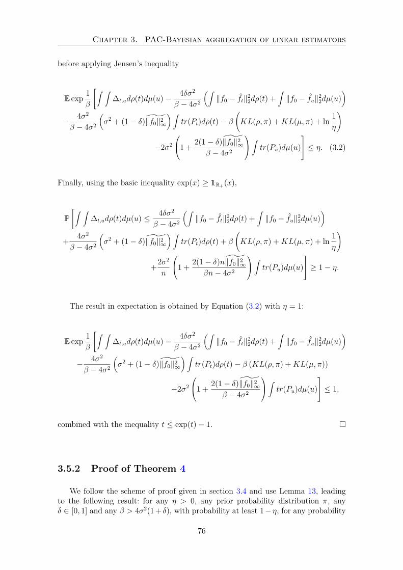
Chapter 3. PAC-Bayesian aggregation of linear estimators
before applying Jensen’s inequality
E exp1β
[∫ ∫∆t,udρ(t)dµ(u) − 4δσ2
β − 4σ2
(∫‖f0 − ft‖2
2dρ(t) +∫
‖f0 − fu‖22dµ(u)
)
− 4σ2
β − 4σ2
(σ2 + (1 − δ)‖f0‖2
∞
) ∫tr(Pt)dρ(t) − β
(KL(ρ, π) +KL(µ, π) + ln
1η
)
−2σ2
1 +
2(1 − δ)‖f0‖2∞
β − 4σ2
∫tr(Pu)dµ(u)
≤ η. (3.2)
Finally, using the basic inequality exp(x) ≥ 1R+(x),
P
[∫ ∫∆t,udρ(t)dµ(u) ≤ 4δσ2
β − 4σ2
(∫‖f0 − ft‖2
2dρ(t) +∫
‖f0 − fu‖22dµ(u)
)
+4σ2
β − 4σ2
(σ2 + (1 − δ)‖f0‖2
∞
) ∫tr(Pt)dρ(t) + β
(KL(ρ, π) +KL(µ, π) + ln
1η
)
+2σ2
n
1 +
2(1 − δ)n‖f0‖2∞
βn− 4σ2
∫tr(Pu)dµ(u)
≥ 1 − η.
The result in expectation is obtained by Equation (3.2) with η = 1:
E exp1β
[∫ ∫∆t,udρ(t)dµ(u) − 4δσ2
β − 4σ2
(∫‖f0 − ft‖2
2dρ(t) +∫
‖f0 − fu‖22dµ(u)
)
− 4σ2
β − 4σ2
(σ2 + (1 − δ)‖f0‖2
∞
) ∫tr(Pt)dρ(t) − β (KL(ρ, π) +KL(µ, π))
−2σ2
1 +
2(1 − δ)‖f0‖2∞
β − 4σ2
∫tr(Pu)dµ(u)
≤ 1,
combined with the inequality t ≤ exp(t) − 1.
3.5.2 Proof of Theorem 4
We follow the scheme of proof given in section 3.4 and use Lemma 13, leadingto the following result: for any η > 0, any prior probability distribution π, anyδ ∈ [0, 1] and any β > 4σ2(1 + δ), with probability at least 1 − η, for any probability
76

3.5. The expository case of Gaussian noise and projection estimates
distribution µ,
∫‖f0 − ft‖2
2dρ(t) −∫
‖f0 − ft‖22dµ(t)
≤ 4δσ2
β − 4σ2
(∫‖f0 − ft‖2
2dρ(t) +∫
‖f0 − fu‖22dµ(u)
)
+4σ2
β − 4σ2
(σ2 + (1 − δ)‖f0‖2
∞
) ∫tr(Pt)dρ(t) −
∫pen(t)dρ(t)
+ 2σ2
1 +
2(1 − δ)‖f0‖2∞
β − 4σ2
∫tr(Pt)dµ(t) +
∫pen(t)dµ(t)
+ β
(2KL(µ, π) + ln
1η
).
With pen(t) ≥ 4σ2
β−4σ2
(σ2 + (1 − δ)‖f0‖2
∞
)tr(Pt), the previous inequality becomes
(1 − 4δσ2
β − 4σ2
)∫‖f0 − ft‖2
2dρ(t) −(
1 +4δσ2
β − 4σ2
)∫‖f0 − ft‖2
2dµ(t)
≤ 2σ2
1 +
2(1 − δ)‖f0‖2∞
β − 4σ2
∫tr(Pt)dµ(t) +
∫pen(t)dµ(t) + β
(2KL(µ, π) + ln
1η
).
Furthermore, using
‖f0 − fEW A‖22 ≤
∫‖f0 − ft‖2
2dρ(t),
if β > 4σ2(δ + 1), we obtain
‖f0 − fEW A‖22 ≤ inf
µ∈M1+(T )
(1 +
8σ2δ
β − 4σ2(δ + 1)
)∫‖f0 − ft‖2
2dµ(t)
+
(1 +
4σ2δ
β − 4σ2(δ + 1)
)2σ2
1 +
2(1 − δ)‖f0‖2∞
β − 4σ2
∫tr(Pt)dµ(t)
+
(1 +
4σ2δ
β − 4σ2(δ + 1)
)∫pen(t)dµ(t)+β
(1 +
4σ2δ
β − 4σ2(δ + 1)
)(2KL(µ, π) + ln
1η
).
In addition, taking ǫ = 4σ2δβ−4σ2(δ+1)
, gives
‖f0 − fEW A‖22 ≤ inf
µ∈M1+(T )
(1 + 2ǫ)∫
‖f0 − ft‖22dµ(t)
+ 2σ2 (1 + ǫ)
1 +
2(1 − δ)‖f0‖2∞
β − 4σ2
∫tr(Pt)dµ(t)
+ (1 + ǫ)
(∫pen(t)dµ(t) + 2βKL(µ, π) + β ln
1η
).
77

Chapter 3. PAC-Bayesian aggregation of linear estimators
3.6 Appendix : Proofs in the sub-Gaussian case
3.6.1 Proof of Theorem 3
The proof follows from the scheme described in section 3.4. The main point isstill to control ∫ (
‖f0 − ft‖22 − rt
)dρ(t) −
∫ (‖f0 − ft‖2
2 − rt
)dµ(t).
We recall that Pt is a symmetric positive semi-definite matrix, there exists V > 0such that supt∈T ‖Pt‖2 ≤ V and W is a centered sub-Gaussian noise. For any t, u ∈T , we still denote ∆t,u = ‖f0 − ft‖2
2 − rt − ‖f0 − fu‖22 + ru.
Lemma 14. Let π be an arbitrary prior probability. For any δ ∈ [0, 1], any β > 4σ2Vand β ≥ 4σ2V (1 + 4δ), let
γ =1
16σ2δV 2
(β − 4σ2V (1 + 2δ) −
√β − 4σ2V
√β − 4σ2V (1 + 4δ)
)1δ>0.
Then, for any probability distributions ρ and µ, for any ν > 0,— for any η ∈ (0, 1], with probability at least 1 − η,
∫ ∫∆t,udρ(t)dµ(u) ≤ (1 + ν)γ
∫‖PtY − f0‖2
2dρ(t)
+4σ2
β − 4σ2V
(σ2 + (1 − δ)(1 + 2γV )2‖f0‖2
∞
) ∫tr(P 2
t )dρ(t)
+ 2σ2
(∫tr(Pu)dµ(u) +
2(1 − δ)(1 + 2γV )2
β − 4σ2V‖f0‖2
∞
∫tr(P 2
u )dµ(u)
)
+(
1 +1ν
)γ∫
‖PuY − f0‖22dµ(u) + β
(KL(ρ, π) +KL(µ, π) + ln
1η
)
— Moreover,
E
[∫ ∫∆t,udρ(t)dµ(u)
]≤ E
[(1 + ν)γ
∫‖PtY − f0‖2
2dρ(t)
+4σ2
β − 4σ2V
(σ2 + (1 − δ)(1 + 2γV )2‖f0‖2
∞
) ∫tr(P 2
t )dρ(t)
+ 2σ2
(∫tr(Pu)dµ(u) +
2(1 − δ)(1 + 2γV )2
β − 4σ2V‖f0‖2
∞
∫tr(P 2
u )dµ(u)
)
+(
1 +1ν
)γ∫
‖PuY − f0‖22dµ(u) + β (KL(ρ, π) +KL(µ, π))
]
Under the assumptions of the previous lemma, with probability at least 1 − η,∫
‖f0 − ft‖22dρ(t) −
∫‖f0 − ft‖2
2dµ(t) ≤ (1 + ν)γ∫
‖ft − f0‖22dρ(t)
+4σ2
β − 4σ2V
(σ2 + (1 − δ)(1 + 2γV )2‖f0‖2
∞
) ∫tr(P 2
t )dρ(t) −∫
pen(t)dρ(t)
+ 2σ2
(∫tr(Pt)dµ(t) +
2(1 − δ)(1 + 2γV )2
β − 4σ2V‖f0‖2
∞
∫tr(P 2
t )dµ(t)
)+∫
pen(t)dµ(t)
+(
1 +1ν
)γ∫
‖ft − f0‖22dµ(t) + β
(2KL(µ, π) + ln
1η
).
78

3.6. Appendix : Proofs in the sub-Gaussian case
Taking pen(t) ≥ 4σ2
β−4σ2V
(σ2 + (1 − δ)(1 + 2γV )2‖f0‖2
∞
)tr(P 2
t ) and ν ∈ N = {ν >0|(1 + ν)γ < 1}, such that the inequality stays informative,
(1 − (1 + ν)γ)∫
‖f0 − ft‖22dρ(t) ≤
(1 +
(1 +
1ν
)γ) ∫
‖f0 − ft‖22dµ(t)
+ 2σ2
(∫tr(Pt)dµ(t) +
2(1 − δ)(1 + 2γV )2
β − 4σ2V‖f0‖2
∞
∫tr(P 2
t )dµ(t)
)
+∫
pen(t)dµ(t) + β
(2KL(µ, π) + ln
1η
).
Finally, since ‖f0 − fEW A‖22 ≤ ∫ ‖f0 − ft‖2
2dρ(t),
‖f0 − fEW A‖22 ≤
(1 +
(1 + ν)2γ
ν(1 − (1 + ν)γ)
)∫‖f0 − ft‖2
2dµ(t)
+2σ2
1 − (1 + ν)γ
(∫tr(Pt)dµ(t) +
2(1 − δ)(1 + 2γV )2
β − 4σ2V‖f0‖2
∞
∫tr(P 2
t )dµ(t)
)
+1
1 − (1 + ν)γ
(∫pen(t)dµ(t) + β
(2KL(µ, π) + ln
1η
)).
The result in expectation is obtained in the same fashion.
3.6.2 Proof of Lemma 14
The exponential moment of ∆t,u is easily controlled by a term involving ‖Ptf0 −f0‖2
2 (see Equation (3.1)). Since Pt are not projections, ‖Ptf0 − f0‖22 ≤ ‖PtY − f0‖2
2
does not hold any more. The presence of ‖PtY − f0‖22 allows us to obtain a weak
oracle inequality. To overcome this difficulty, ‖(Pt − Pu)Y ‖22 is introduced and for
an arbitrary γ ≥ 0, we try to control ∆t,u − γ‖(Pt − Pu)Y ‖22.
Proof. A simple calculation yields
∆t,u − γ‖(Pt − Pu)Y ‖22 = W⊤(2I − γ(Pt − Pu)⊤)(Pt − Pu)W
+ 2W⊤(I − γ(Pt − Pu)⊤)(Pt − Pu)f0 − 2σ2tr(Pt − Pu) − γ‖(Pt − Pu)f0‖22.
Noting that W⊤(2I−γ(Pt −Pu)⊤)(Pt −Pu)W ≤ 2W⊤(Pt −Pu)W and since (Pt)t∈Tare positive semi-definite matrices, 2W⊤(Pt − Pu)W ≤ 2W⊤PtW . Thus, for anyβ > 0, any γ ≥ 0,
E exp
(∆t,u
β− γ
β‖(Pt − Pu)Y ‖2
2
)
≤ E
[exp
2β
(W⊤PtW +W⊤(I − γ(Pt − Pu))(Pt − Pu)f0
)]
× exp−1β
(2σ2tr(Pt − Pu) + γ‖(Pt − Pu)f0‖2
2
).
79

Chapter 3. PAC-Bayesian aggregation of linear estimators
The first step is to bring us back to the Gaussian case, using W ’s sub-Gaussianityand an idea of Hsu et al. [2012]. Let Z be a standard Gaussian random variable,independent of W . Then,
E exp
(2√βW⊤
√PtZ +
2βW⊤(I − γ(Pt − Pu))(Pt − Pu)f0
)
= E
[E
[exp
(2√βW⊤
√PtZ +
2βW⊤(I − γ(Pt − Pu))(Pt − Pu)f0
) ∣∣∣W]]
= E
[E
[exp
(2√βW⊤
√PtZ
) ∣∣∣W]
exp
(2βW⊤(I − γ(Pt − Pu))(Pt − Pu)f0
)]
= E exp2β
(W⊤PtW +W⊤(I − γ(Pt − Pu))(Pt − Pu)f0
).
On the other hand,
E
[exp
2β
(W⊤PtW +W⊤(I − γ(Pt − Pu))(Pt − Pu)f0
)]
= E
[E
[exp
(2√βW⊤
√PtZ +
2βW⊤(I − γ(Pt − Pu))(Pt − Pu)f0
) ∣∣∣Z]].
Since W is sub-Gaussian with parameter σ,
E
[exp
2β
(W⊤PtW +W⊤(I − γ(Pt − Pu))(Pt − Pu)f0
)]
≤ E exp
σ
2
2
∥∥∥∥∥2√β
(√PtZ +
1√β
(I − γ(Pt − Pu))(Pt − Pu)f0
)∥∥∥∥∥
2
2
Hence,
E exp
(∆t,u
β− γ
β‖(Pt − Pu)Y ‖2
2
)
≤ E
[exp
2σ2
β
(Z⊤PtZ +
2√βZ⊤
√Pt(I − γ(Pt − Pu))(Pt − Pu)f0
)]
×exp
(2σ2
β2‖(I − γ(Pt − Pu))(Pt − Pu)f0‖2
2 − 2σ2
βtr(Pt − Pu) − γ
β‖(Pt − Pu)f0‖2
2
).
The expectation is similar to the one obtained in the Gaussian case: the exponentialof some quadratic form. The same recipe is applied. Since Pt is positive semi-definite,there exist an orthogonal matrix U and a diagonal matrix D such that Pt = U⊤DU.Note that UZ is a standard Gaussian variable. This diagonalization step and thenon-negativity of the eigenvalues allow to apply Lemma 2.4 of Hsu et al. [2012].
80

3.6. Appendix : Proofs in the sub-Gaussian case
Then, for any β > 4σ2V , any γ ≥ 0,
E exp
(∆t,u
β− γ
β‖(Pt − Pu)Y ‖2
2
)
≤ exp2σ2
β
(tr(Pt) +
2σ2
β(β − 4σ2V )
(βtr(P 2
t ) + 2∥∥∥∥√Pt(I − γ(Pt − Pu))(Pt − Pu)f0
∥∥∥∥2
2
))
×exp
(2σ2
β2‖(I − γ(Pt − Pu))(Pt − Pu)f0‖2
2 − 2σ2
βtr(Pt − Pu) − γ
β‖(Pt − Pu)f0‖2
2
).
Consequently,
E exp
(∆t,u
β+γ
β
(‖(Pt − Pu)f0‖2
2 − ‖(Pt − Pu)Y ‖22
))
≤ exp2σ2
β
(tr(Pu) +
2σ2
β − 4σ2Vtr(P 2
t )
)
× exp
(2σ2
β2
(4σ2V
β − 4σ2V(1 + 2γV )2 + (1 + 2γV )2
)‖(Pt − Pu)f0‖2
2
).
≤ exp2σ2
β
(tr(Pu) +
2σ2
β − 4σ2Vtr(P 2
t ) +(1 + 2γV )2
β − 4σ2V‖(Pt − Pu)f0‖2
2
).
If an exact oracle inequality is wished, ‖(Pt − Pu)f0‖22 should be upper bounded
by some constant and γ should be set to zero. Else, γ is used to replace the termsin ‖(Pt −Pu)f0‖2
2 by ‖(Pt −Pu)Y ‖22. Thus, the terms depending on f0 will be upper
bounded in two ways:
— on the one hand, using ‖f0‖2∞
‖(Pt − Pu)f0‖22 ≤ 2
(‖Ptf0‖2
2 + ‖Puf0‖22
)≤ 2
(tr(P 2
t ) + tr(P 2u ))
‖f0‖2∞
For any δ ∈ [0, 1],
E exp
(∆t,u
β+γ
β
(‖(Pt − Pu)f0‖2
2 − ‖(Pt − Pu)Y ‖22
))
≤ exp2σ2
β
(tr(Pu) +
2σ2
β − 4σ2Vtr(P 2
t ) +(1 + 2γV )2(1 − δ)
β − 4σ2V‖(Pt − Pu)f0‖2
2
)
× exp
(2σ2(1 + 2γV )2δ
β(β − 4σ2V )‖(Pt − Pu)f0‖2
n
)
≤ exp2σ2
β
(tr(Pu) +
2σ2
β − 4σ2Vtr(P 2
t ) +(1 + 2γV )2δ
β − 4σ2V‖(Pt − Pu)f0‖2
2
)
× exp
(4σ2(1 + 2γV )2(1 − δ)
β(β − 4σ2V )
(tr(P 2
t ) + tr(P 2u ))
‖f0‖2∞
).
— on the other hand, introducing ‖PtY −f0‖22 to obtain a weak oracle inequality:
conditions should be found on γ such that
2σ2(1 + 2γV )2δ
β − 4σ2V‖(Pt − Pu)f0‖2
2 − γ(‖(Pt − Pu)f0‖2
2 − ‖(Pt − Pu)Y ‖22
)
≤ C1‖PtY − f0‖22 + C2‖PuY − f0‖2
2
81

Chapter 3. PAC-Bayesian aggregation of linear estimators
for some non-negative constants C1 and C2 and with δ > 0. Since for anyν > 0, ‖(Pt −Pu)Y ‖2
2 ≤ (1 + ν)‖PtY − f0‖22 +
(1 + 1
ν
)‖PuY − f0‖2
2, it sufficesthat
2σ2(1 + 2γV )2δ
β − 4σ2V‖(Pt − Pu)f0‖2
2 − γ‖(Pt − Pu)f0‖22 ≤ 0.
This condition may be fulfilled if β ≥ 4σ2V (1 + 4δ). The smallest γ ≥ 0among all the possible ones is chosen :
γ =1
16σ2δV 2
(β − 4σ2V (1 + 2δ) −
√β − 4σ2V
√β − 4σ2V (1 + 4δ)
)1δ>0.
This leads to the following inequality : for any δ ∈ [0, 1], for any β > 4σ2V andβ ≥ 4σ2V (1 + 4δ), with γ previously defined, for any ν > 0,
E exp
(∆t,u
β− γ
β
((1 + ν)‖PtY − f0‖2
2 +(
1 +1ν
)‖PuY − f0‖2
2
))
≤ exp2σ2
β
(tr(Pu) +
2σ2
β − 4σ2Vtr(P 2
t ) +2(1 + 2γV )2(1 − δ)
β − 4σ2V
(tr(P 2
t ) + tr(P 2u ))
‖f0‖2∞
).
The rest of the proof follows the same steps as in the Gaussian case: we firstintegrate according to the prior π, use Fubini’s theorem, introduce the probabilitymeasures ρ and µ and apply Jensen’s inequality to obtain that for any η ∈ (0, 1],
E exp1β
[ ∫ ∫∆t,udρ(t)dµ(u) − (1 + ν)γ
∫‖PtY − f0‖2
2dρ(t)
− 4σ2
β − 4σ2V
(σ2 + (1 − δ)(1 + 2γV )2‖f0‖2
∞
) ∫tr(P 2
t )dρ(t)
− 2σ2
(∫tr(Pu)dµ(u) +
2(1 − δ)(1 + 2γV )2
β − 4σ2V‖f0‖2
∞
∫tr(P 2
u )dµ(u)
)
−(
1 +1ν
)γ∫
‖PuY − f0‖22dµ(u)
− β
(KL(ρ, π) +KL(µ, π) + ln
1η
) ]≤ η. (3.3)
Finally, using exp(x) ≥ 1R+(x), for any δ ∈ [0, 1], any β > 4σ2V and β ≥ 4σ2V (1 +4δ), with γ previously defined, for any η ∈ (0, 1], for any ν > 0,
P
[ ∫ ∫∆t,udρ(t)dµ(u) ≤ (1 + ν)γ
∫‖PtY − f0‖2
2dρ(t)
+4σ2
β − 4σ2V
(σ2 + (1 − δ)(1 + 2γV )2‖f0‖2
∞
) ∫tr(P 2
t )dρ(t)
+ 2σ2
(∫tr(Pu)dµ(u) +
2(1 − δ)(1 + 2γV )2
β − 4σ2V‖f0‖2
∞
∫tr(P 2
u )dµ(u)
)
+(
1 +1ν
)γ∫
‖PuY − f0‖22dµ(u) + β
(KL(ρ, π) +KL(µ, π) + ln
1η
) ]≥ 1 − η.
The result in expectation comes from Equation (3.3) with η = 1, combined with theinequality t ≤ exp(t) − 1.
82

Bibliography
H. Akaike. Information theory and an extension of the maximum likelihood principle.In Second International Symposium on Information Theory (Tsahkadsor, 1971),pages 267–281. Akadémiai Kiadó, Budapest, 1973. 15
N. Akakpo and C. Lacour. Inhomogeneous and anisotropic conditional density es-timation from dependent data. Electron. J. Stat., 5:1618–1653, 2011. ISSN 1935-7524. doi: 10.1214/11-EJS653. URL http://dx.doi.org/10.1214/11-EJS653.13
D. M. Allen. The relationship between variable selection and data augmentationand a method for prediction. Technometrics, 16:125–127, 1974. ISSN 0040-1706.15
P. Alquier and K. Lounici. PAC-Bayesian bounds for sparse regression estimationwith exponential weights. Electron. J. Stat., 5:127–145, 2011. ISSN 1935-7524.doi: 10.1214/11-EJS601. URL http://dx.doi.org/10.1214/11-EJS601. 75
Y. Amit and D. Geman. Shape quantization and recognition with randomizedtrees. Neural Comput., 9(7):1545–1588, October 1997. ISSN 0899-7667. doi:10.1162/neco.1997.9.7.1545. URL http://dx.doi.org/10.1162/neco.1997.9.
7.1545. 16, 66
A. Antoniadis, J. Bigot, and R. von Sachs. A multiscale approach for statisticalcharacterization of functional images. Journal of Computational and GraphicalStatistics, 18, 2009. 19, 25
S. Arlot. V-fold cross-validation improved: V-fold penalization. 40 pages, plus aseparate technical appendix., 2008. URL http://hal.archives-ouvertes.fr/
hal-00239182. 15
S. Arlot and A. Celisse. A survey of cross-validation procedures for model selection.Stat. Surv., 4:40–79, 2010. ISSN 1935-7516. doi: 10.1214/09-SS054. URL http:
//dx.doi.org.revues.math.u-psud.fr:2048/10.1214/09-SS054. 15
J.-Y. Audibert. Aggregated estimators and empirical complexity for least square re-gression. Ann. Inst. H. Poincaré Probab. Statist., 40(6):685–736, 2004. ISSN 0246-0203. doi: 10.1016/j.anihpb.2003.11.006. URL http://dx.doi.org/10.1016/j.
anihpb.2003.11.006. 18
J.-Y. Audibert. Progressive mixture rules are deviation suboptimal. In Advances inNeural Information Processing Systems, 2008. 21

Bibliography
A. Barron, L. Birgé, and P. Massart. Risk bounds for model selection via penaliza-tion. Probab. Theory Related Fields, 113(3):301–413, 1999. ISSN 0178-8051. doi:10.1007/s004400050210. URL http://dx.doi.org.revues.math.u-psud.fr:
2048/10.1007/s004400050210. 15
A. Barron, C. Huang, J. Li, and X. Luo. The mdl principle, penalized likelihoods,and statistical risk. Festschrift for Jorma Rissanen. Tampere University Press,Tampere, Finland, 2008. 31
D. M. Bashtannyk and R. J. Hyndman. Bandwidth selection for kernel conditionaldensity estimation. Comput. Statist. Data Anal., 36(3):279–298, 2001. ISSN 0167-9473. doi: 10.1016/S0167-9473(00)00046-3. URL http://dx.doi.org.revues.
math.u-psud.fr:2048/10.1016/S0167-9473(00)00046-3. 12
J.-P. Baudry, C. Maugis, and B. Michel. Slope heuristics: Overview and implemen-tation. Statistics and Computing, 22, 2011. 34
P. Bellec. Concentration of quadratic forms and aggregation of affine estimators.ArXiv e-prints, October 2014. 66
A. Belloni, V. Chernozhukov, and L. Wang. Square-root lasso: pivotal recovery ofsparse signals via conic programming. Biometrika, 98(4):791–806, 2011. ISSN0006-3444. doi: 10.1093/biomet/asr043. URL http://dx.doi.org/10.1093/
biomet/asr043. 21, 66
J. O. Berger and L. R. Pericchi. The intrinsic Bayes factor for model selection andprediction. J. Amer. Statist. Assoc., 91(433):109–122, 1996. ISSN 0162-1459. doi:10.2307/2291387. URL http://dx.doi.org/10.2307/2291387. 15
G. Biau. Analysis of a random forests model. J. Mach. Learn. Res., 13:1063–1095,2012. ISSN 1532-4435. 16, 66
G. Biau and L. Devroye. On the layered nearest neighbour estimate, the baggednearest neighbour estimate and the random forest method in regression and clas-sification. J. Multivariate Anal., 101(10):2499–2518, 2010. ISSN 0047-259X. doi:10.1016/j.jmva.2010.06.019. URL http://dx.doi.org/10.1016/j.jmva.2010.
06.019. 16, 66
G. Biau, L. Devroye, and G. Lugosi. Consistency of random forests and otheraveraging classifiers. J. Mach. Learn. Res., 9:2015–2033, 2008. ISSN 1532-4435.16, 66
C. Biernacki and G. Castellan. A data-driven bound on variances for avoidingdegeneracy in univariate gaussian mixtures. Pub IRMA Lille, 71, 2011. 34
L. Birgé and P. Massart. Minimal penalties for gaussian model selection. ProbabilityTheory and Related Fields, 138(1-2):33–73, 2007. ISSN 0178-8051. doi: 10.1007/s00440-006-0011-8. 34
G. Blanchard, C. Schäfer, Y. Rozenholc, and K. R. Müller. Optimal dyadic decisiontrees. Machine Learning, 66(2):209–241, 2007. 13
84

Bibliography
L. Breiman. Bagging predictors. Machine Learning, 24(2):123–140, 1996. ISSN0885-6125. doi: 10.1023/A:1018054314350. 16, 66
L. Breiman. Random forests. Machine Learning, 45(1):5–32, 2001. ISSN 0885-6125.doi: 10.1023/A:1010933404324. 16, 66
N. D Brinkman. Ethanol fuel-a single-cylinder engine study of efficiency and exhaustemissions. SAE Technical Paper, 810345, 1981. 20, 26, 37
E. Brunel, F. Comte, and C. Lacour. Adaptive estimation of the conditional densityin presence of censoring. Sankhya, 69(Part 4.):pages 734–763, December 2007.URL http://hal.archives-ouvertes.fr/hal-00152794. 13
F. Bunea, A. B. Tsybakov, and M. H. Wegkamp. Aggregation for Gaussian re-gression. Ann. Statist., 35(4):1674–1697, 2007. ISSN 0090-5364. doi: 10.1214/009053606000001587. URL http://dx.doi.org/10.1214/009053606000001587.17
K. P. Burnham and D. R. Anderson. Model selection and multimodel inference. Apractical information-theoretic approach. Springer-Verlag, New-York, 2nd edition,2002. 18, 25
O. Catoni. Statistical learning theory and stochastic optimization, volume 1851 ofLecture Notes in Mathematics. Springer-Verlag, Berlin, 2004. ISBN 3-540-22572-2. doi: 10.1007/b99352. URL http://dx.doi.org/10.1007/b99352. Lecturenotes from the 31st Summer School on Probability Theory held in Saint-Flour,July 8–25, 2001. 17, 18, 66
O. Catoni. Pac-Bayesian supervised classification: the thermodynamics of statisticallearning. Institute of Mathematical Statistics Lecture Notes—Monograph Series,56. Institute of Mathematical Statistics, Beachwood, OH, 2007. ISBN 978-0-940600-72-0; 0-940600-72-2. 17, 18, 66, 72
G. Celeux and G. Govaert. Gaussian parsimonious clustering models. PatternRecognition, 28(5), 1995. 30, 33, 34
A. Celisse. Optimal cross-validation in density estimation. 2008. URL http://hal.
archives-ouvertes.fr/hal-00337058. 15
N. Cesa-Bianchi and G. Lugosi. On prediction of individual sequences. Ann. Statist.,27(6):1865–1895, 1999. ISSN 0090-5364. doi: 10.1214/aos/1017939242. URLhttp://dx.doi.org/10.1214/aos/1017939242. 16, 66
N. Cesa-Bianchi, Y. Freund, D. Haussler, D. P. Helmbold, R. E. Schapire, and M. K.Warmuth. How to use expert advice. J. ACM, 44(3):427–485, May 1997. ISSN0004-5411. doi: 10.1145/258128.258179. URL http://doi.acm.org/10.1145/
258128.258179. 16, 66
F. Chamroukhi, A. Samé, G. Govaert, and P. Aknin. Time series modelling by aregression approach based on a latent process. Neural Networks, 22:593–602, 2009.20
85

Bibliography
F. Chamroukhi, A. Samé, G. Govaert, and P. Aknin. A hidden process regressionmodel for functional data description. application to curve discrimination. Neu-rocomputing, 73:1210–1221, March 2010. 20, 26, 27, 33
T. Choi. Convergence of posterior distribution in the mixture of regressions. Journalof Nonparametric Statistics, 20(4):337–351, may 2008. 19, 25
S. X. Cohen and E. Le Pennec. Conditional density estimation by penalized like-lihood model selection and applications. Technical report, INRIA, 2011. 20, 27,28, 42, 43, 48, 51, 59, 60
S. X. Cohen and E. Le Pennec. Partition-based conditional density estima-tion. ESAIM: Probability and Statistics, 17:672–697, 1 2013. ISSN 1262-3318.doi: 10.1051/ps/2012017. URL http://www.esaim-ps.org/action/article_
S1292810012000171. 13, 19, 25, 41
D. Dai, P. Rigollet, and T. Zhang. Deviation optimal learning using greedy Q-aggregation. Ann. Statist., 40(3):1878–1905, 2012. ISSN 0090-5364. doi: 10.1214/12-AOS1025. URL http://dx.doi.org/10.1214/12-AOS1025. 21, 66
D. Dai, P. Rigollet, L. Xia, and T. Zhang. Aggregation of affine estimators. Electron.J. Stat., 8:302–327, 2014. ISSN 1935-7524. doi: 10.1214/14-EJS886. URL http:
//dx.doi.org/10.1214/14-EJS886. 21, 66, 67, 69
A. S. Dalalyan. SOCP based variance free Dantzig selector with application to robustestimation. C. R. Math. Acad. Sci. Paris, 350(15-16):785–788, 2012. ISSN 1631-073X. doi: 10.1016/j.crma.2012.09.016. URL http://dx.doi.org/10.1016/j.
crma.2012.09.016. 21, 66
A. S. Dalalyan and J. Salmon. Sharp oracle inequalities for aggregation of affineestimators. Ann. Statist., 40(4):2327–2355, 2012. ISSN 0090-5364. doi: 10.1214/12-AOS1038. URL http://dx.doi.org/10.1214/12-AOS1038. 18, 21, 66, 67, 69
A. S. Dalalyan and A. B. Tsybakov. Aggregation by exponential weight-ing and sharp oracle inequalities. In NaderH. Bshouty and Claudio Gen-tile, editors, Learning Theory, volume 4539 of Lecture Notes in Computer Sci-ence, pages 97–111. Springer Berlin Heidelberg, 2007. ISBN 978-3-540-72925-9. doi: 10.1007/978-3-540-72927-3_9. URL http://dx.doi.org/10.1007/
978-3-540-72927-3_9. 17, 66
A. S. Dalalyan and A. B. Tsybakov. Aggregation by exponential weighting, sharppac-bayesian bounds and sparsity. Machine Learning, 72(1-2):39–61, 2008. doi: 10.1007/s10994-008-5051-0. URL http://certis.enpc.fr/~dalalyan/Download/
Dal_Tsyb2008.pdf. 17, 66
A. S. Dalalyan and A. B. Tsybakov. Sparse regression learning by aggregation andLangevin Monte-Carlo. J. Comput. System Sci., 78(5):1423–1443, 2012. ISSN0022-0000. doi: 10.1016/j.jcss.2011.12.023. URL http://dx.doi.org/10.1016/
j.jcss.2011.12.023. 17, 66
86

Bibliography
A. S. Dalalyan, M. Hebiri, K. Meziani, and J. Salmon. Learning heteroscedasticmodels by convex programming under group sparsity. In ICML, 2013. URLpapers/ICML13_DHMS.pdf. 21, 66
J. G. De Gooijer and D. Zerom. On conditional density estimation. Statist.Neerlandica, 57(2):159–176, 2003. ISSN 0039-0402. doi: 10.1111/1467-9574.00226. URL http://dx.doi.org.revues.math.u-psud.fr:2048/10.1111/
1467-9574.00226. 12
A. P. Dempster, N. M. Laird, and D. B. Rubin. Maximum likelihood from incompletedata via the em algorithm. Journal of the Royal Statistical Society. Series B., 39(1), 1977. 33
D. L. Donoho and I. M. Johnstone. Ideal spatial adaptation by wavelet shrinkage.Biometrika, 81(3):425–455, 1994. ISSN 0006-3444. doi: 10.1093/biomet/81.3.425.URL http://dx.doi.org/10.1093/biomet/81.3.425. 16
D. L. Donoho and I. M. Johnstone. Minimax estimation via wavelet shrinkage. Ann.Statist., 26(3):879–921, 1998. ISSN 0090-5364. doi: 10.1214/aos/1024691081. URLhttp://dx.doi.org/10.1214/aos/1024691081. 14
D. L. Donoho, I. M. Johnstone, G. Kerkyacharian, and D. Picard. Wavelet shrink-age: asymptopia? J. Roy. Statist. Soc. Ser. B, 57(2):301–369, 1995. ISSN 0035-9246. URL http://links.jstor.org/sici?sici=0035-9246(1995)57:2<301:
WSA>2.0.CO;2-S&origin=MSN. With discussion and a reply by the authors. 12,16
S. Efromovich. Oracle inequality for conditional density estimation and an ac-tuarial example. Ann. Inst. Statist. Math., 62(2):249–275, 2010. ISSN 0020-3157. doi: 10.1007/s10463-008-0185-1. URL http://dx.doi.org/10.1007/
s10463-008-0185-1. 13
J. Fan and I. Gijbels. Local polynomial modelling and its applications, volume 66of Monographs on Statistics and Applied Probability. Chapman & Hall, London,1996. ISBN 0-412-98321-4. 12
J. Fan and T. H. Yim. A crossvalidation method for estimating conditional densities.Biometrika, 91(4):819–834, 2004. ISSN 0006-3444. doi: 10.1093/biomet/91.4.819.URL http://dx.doi.org/10.1093/biomet/91.4.819. 12
J. Fan, Q. Yao, and H. Tong. Estimation of conditional densities and sensitivitymeasures in nonlinear dynamical systems. Biometrika, 83(1):189–206, 1996. ISSN0006-3444. doi: 10.1093/biomet/83.1.189. URL http://dx.doi.org/10.1093/
biomet/83.1.189. 12
Y. Freund. Boosting a weak learning algorithm by majority. Inform. and Comput.,121(2):256–285, 1995. ISSN 0890-5401. doi: 10.1006/inco.1995.1136. URL http:
//dx.doi.org/10.1006/inco.1995.1136. 16, 66
87

Bibliography
S. Gaïffas and G. Lecué. Hyper-sparse optimal aggregation. J. Mach. Learn. Res.,12:1813–1833, 2011. ISSN 1532-4435. 21
E. Gassiat and R. van Handel. The local geometry of finite mixtures. Trans. Amer.Math. Soc., 366(2):1047–1072, 2014. 32
Y. Ge and W. Jiang. On consistency of bayesian inference with mixtures of logisticregression. Neural Computation, 18(1):224–243, January 2006. 19, 25
S. Geisser. The predictive sample reuse method with applications. Journal of theAmerican Statistical Association, 70(350):pp. 320–328, 1975. ISSN 01621459. URLhttp://www.jstor.org/stable/2285815. 15
C. Genovese and L. Wasserman. Rates of convergence for the gaussian mixture sieve.The Annals of Statistics, 28(4):1105–1127, august 2000. 19, 25
R. Genuer. Forêts aléatoires : aspects théoriques, sélection de variables et applica-tions. PhD thesis, Université Paris-Sud, 2011. 16, 66
C. Giraud. Mixing least-squares estimators when the variance is unknown. Bernoulli,14(4):1089–1107, 2008. ISSN 1350-7265. doi: 10.3150/08-BEJ135. URL http:
//dx.doi.org/10.3150/08-BEJ135. 21, 66
C. Giraud, S. Huet, and N. Verzelen. High-dimensional regression with un-known variance. Statist. Sci., 27(4):500–518, 2012. ISSN 0883-4237. doi:10.1214/12-STS398. URL http://dx.doi.org/10.1214/12-STS398. 21, 66
A. Goldenshluger and O. Lepski. Bandwidth selection in kernel density estimation:oracle inequalities and adaptive minimax optimality. Ann. Statist., 39(3):1608–1632, 2011. ISSN 0090-5364. doi: 10.1214/11-AOS883. URL http://dx.doi.
org.revues.math.u-psud.fr:2048/10.1214/11-AOS883. 15
B. Guedj and P. Alquier. PAC-Bayesian estimation and prediction in sparseadditive models. Electron. J. Stat., 7:264–291, 2013. ISSN 1935-7524. doi:10.1214/13-EJS771. URL http://dx.doi.org/10.1214/13-EJS771. 69
L. Györfi and M. Kohler. Nonparametric estimation of conditional distributions.IEEE Trans. Inform. Theory, 53(5):1872–1879, 2007. ISSN 0018-9448. doi: 10.1109/TIT.2007.894631. URL http://dx.doi.org/10.1109/TIT.2007.894631.13
L. Györfi, M. Kohler, A. Krzyzak, and H. Walk. A distribution-free theory ofnonparametric regression. Springer series in statistics. Springer, New York,Berlin, Paris, 2002. ISBN 0-387-95441-4. URL http://opac.inria.fr/record=
b1123996. Autre(s) tirage(s) : 2010. 12
P. Hall, R. C. L. Wolff, and Q. Yao. Methods for estimating a conditional distri-bution function. J. Amer. Statist. Assoc., 94(445):154–163, 1999. ISSN 0162-1459. doi: 10.2307/2669691. URL http://dx.doi.org.revues.math.u-psud.
fr:2048/10.2307/2669691. 12
88

Bibliography
P. Hall, J. Racine, and Q. Li. Cross-validation and the estimation of conditionalprobability densities. J. Amer. Statist. Assoc., 99(468):1015–1026, 2004. ISSN0162-1459. doi: 10.1198/016214504000000548. URL http://dx.doi.org/10.
1198/016214504000000548. 12
T. Hastie, R. Tibshirani, and J. Friedman. The elements of statistical learning.Springer Series in Statistics. Springer, New York, second edition, 2009. ISBN978-0-387-84857-0. doi: 10.1007/978-0-387-84858-7. URL http://dx.doi.org.
revues.math.u-psud.fr:2048/10.1007/978-0-387-84858-7. Data mining, in-ference, and prediction. 13, 16
D. Hsu, S. M. Kakade, and T. Zhang. A tail inequality for quadratic forms ofsubgaussian random vectors. Electron. Commun. Probab., 17:no. 52, 6, 2012.ISSN 1083-589X. doi: 10.1214/ECP.v17-2079. URL http://dx.doi.org/10.
1214/ECP.v17-2079. 75, 80
M. Huang and W. Yao. Mixture of regression models with varying mixing propor-tions: a semiparametric approach. J. Amer. Statist. Assoc., 107(498):711–724,2012. ISSN 0162-1459. doi: 10.1080/01621459.2012.682541. 19, 25
M. Huang, R. Li, and S. Wang. Nonparametric mixtures of regressions models.Journal of the American Statistical Association, 108(503):929–941, 2013. 19, 25
D. R. Hunter and D. S. Young. Semiparametric mixtures of regressions. J. Non-parametr. Stat., 24(1):19–38, 2012. ISSN 1048-5252. doi: 10.1080/10485252.2011.608430. 19, 25
R. J. Hyndman and Q. Yao. Nonparametric estimation and symmetry tests forconditional density functions. J. Nonparametr. Stat., 14(3):259–278, 2002. ISSN1048-5252. doi: 10.1080/10485250212374. URL http://dx.doi.org.revues.
math.u-psud.fr:2048/10.1080/10485250212374. 12
R. J. Hyndman, D. M. Bashtannyk, and G. K. Grunwald. Estimating and visualizingconditional densities. J. Comput. Graph. Statist., 5(4):315–336, 1996. ISSN 1061-8600. doi: 10.2307/1390887. URL http://dx.doi.org/10.2307/1390887. 12
M. I. Jordan and R. A. Jacobs. Hierarchical mixtures of experts and the em al-gorithm. In Maria Marinaro and PietroG. Morasso, editors, ICANN 94, pages479–486. Springer London, 1994. ISBN 978-3-540-19887-1. 19, 25
R. E. Kass and A. E. Raftery. Bayes factors. Journal of the American Sta-tistical Association, 90(430):pp. 773–795, 1995. ISSN 01621459. URL http:
//www.jstor.org/stable/2291091. 15
E. D. Kolaczyk, J. Ju, and S. Gopal. Multiscale, multigranular statistical imagesegmentation. Journal of the American Statistical Association, 100:1358–1369,2005. 19, 25
G. Lecué. Optimal rates of aggregation in classification under low noise assumption.Bernoulli, 13(4):1000–1022, 2007. ISSN 1350-7265. doi: 10.3150/07-BEJ6044.URL http://dx.doi.org/10.3150/07-BEJ6044. 17, 66
89

Bibliography
G. Lecué and S. Mendelson. Aggregation via empirical risk minimization. Probab.Theory Related Fields, 145(3-4):591–613, 2009. ISSN 0178-8051. doi: 10.1007/s00440-008-0180-8. URL http://dx.doi.org/10.1007/s00440-008-0180-8. 21
H. K. H. Lee. Consistency of posterior distributions for neural networks. NeuralNetworks, 13:629–642, july 2000. 19, 25
A. M. Legendre. Nouvelles méthodes pour la détermination des orbites des comètes.Firmin Didot, Paris, 1805. "Sur la Méthode des moindres quarrés" appears as anappendix. 13
G. Leung. Improving regression through model mixing. ProQuest LLC, AnnArbor, MI, 2004. ISBN 978-0496-72534-2. URL http://gateway.proquest.
com/openurl?url_ver=Z39.88-2004&rft_val_fmt=info:ofi/fmt:kev:mtx:
dissertation&res_dat=xri:pqdiss&rft_dat=xri:pqdiss:3125244. Thesis(Ph.D.)–Yale University. 18, 21
G. Leung and A. R. Barron. Information theory and mixing least-squares regressions.IEEE Trans. Inform. Theory, 52(8):3396–3410, 2006. ISSN 0018-9448. doi: 10.1109/TIT.2006.878172. URL http://dx.doi.org/10.1109/TIT.2006.878172.17, 66
Q. Li and J. S. Racine. Nonparametric Econometrics: Theory and Practice. Prince-ton University Press, 2007. ISBN 9780691121611. URL http://books.google.
fr/books?id=BI_PiWazY0YC. 12, 19
N. Littlestone and M. K. Warmuth. The weighted majority algorithm. In-formation and Computation, 108(2):212 – 261, 1994. ISSN 0890-5401. doi:http://dx.doi.org/10.1006/inco.1994.1009. URL http://www.sciencedirect.
com/science/article/pii/S0890540184710091. 16, 66
K. Lounici. Generalized mirror averaging and D-convex aggregation. Math. MethodsStatist., 16(3):246–259, 2007. ISSN 1066-5307. doi: 10.3103/S1066530707030040.URL http://dx.doi.org/10.3103/S1066530707030040. 17, 66
C. L. Mallows. Some comments on cp. Technometrics, 15(4):pp. 661–675, 1973.ISSN 00401706. URL http://www.jstor.org/stable/1267380. 15
M. L. Martin-Magniette, T. Mary-Huard, C. Bérard, and S. Robin. Chipmix: mix-ture model of regressions for two-color chip-chip analysis. Bioinformatics, 24(16):i181–i186, 2008. doi: 10.1093/bioinformatics/btn280. 20, 40
P. Massart. Concentration inequalities and model selection, volume 1896 of LectureNotes in Mathematics. Springer, Berlin, 2007. ISBN 978-3-540-48497-4; 3-540-48497-3. Lectures from the 33rd Summer School on Probability Theory held inSaint-Flour, July 6–23, 2003, With a foreword by Jean Picard. 15, 16, 18
P. Massart and C. Meynet. The Lasso as an ℓ1-ball model selection procedure.Electron. J. Stat., 5:669–687, 2011. ISSN 1935-7524. doi: 10.1214/11-EJS623.URL http://dx.doi.org/10.1214/11-EJS623. 16, 17
90

Bibliography
P. Massart and É. Nédélec. Risk bounds for statistical learning. Ann. Statist., 34(5):2326–2366, 2006. ISSN 0090-5364. doi: 10.1214/009053606000000786. URLhttp://dx.doi.org/10.1214/009053606000000786. 13
C. Maugis and B. Michel. A non asymptotic penalized criterion for gaussian mixturemodel selection. ESAIM Probability and Statistics, 2011. 18, 25, 54
C. Maugis and B. Michel. Adaptive density estimation using finite gaussian mixtures.ESAIM Probability and Statistics, 2012. Accepted for publication. 37
D. A. McAllester. Some pac-bayesian theorems. In Proceedings of the EleventhAnnual Conference on Computational Learning Theory, COLT’ 98, pages 230–234, New York, NY, USA, 1998. ACM. ISBN 1-58113-057-0. doi: 10.1145/279943.279989. URL http://doi.acm.org/10.1145/279943.279989. 18
P. McCullagh and J. A. Nelder. Generalized linear models. Monographs on Statisticsand Applied Probability. Chapman & Hall, London, 1983. ISBN 0-412-23850-0. doi: 10.1007/978-1-4899-3244-0. URL http://dx.doi.org.revues.math.
u-psud.fr:2048/10.1007/978-1-4899-3244-0. 13
G. McLachlan and D. Peel. Finite Mixture Models. Wiley, 2000. 19, 25
L. Montuelle and E. Le Pennec. Mixture of gaussian regressions model with logisticweights, a penalized maximum likelihood approach. Electron. J. Statist., 8(1):1661–1695, 2014. ISSN 1935-7524. doi: 10.1214/14-EJS939. 23
É. Nadaraya. On non-parametric estimates of density functions and regressioncurves. Theory of Probability & Its Applications, 10(1):186–190, 1965. doi:10.1137/1110024. URL http://dx.doi.org/10.1137/1110024. 12
A. Nemirovski. Topics in non-parametric statistics. In Lectures on probability theoryand statistics (Saint-Flour, 1998), volume 1738 of Lecture Notes in Math., pages85–277. Springer, Berlin, 2000. 17, 66
A. E. Raftery, D. Madigan, and J. A. Hoeting. Bayesian model averaging for linearregression models. J. Amer. Statist. Assoc., 92(437):179–191, 1997. ISSN 0162-1459. doi: 10.2307/2291462. URL http://dx.doi.org/10.2307/2291462. 15
C. R. Rao and Y. Wu. On model selection, volume 38 of Lecture Notes–MonographSeries, pages 1–57. Institute of Mathematical Statistics, Beachwood, OH,2001. doi: 10.1214/lnms/1215540960. URL http://dx.doi.org/10.1214/lnms/
1215540960. 15
P. Rigollet. Inégalités d’oracle, agrégration et adaptation. PhD thesis, UniversitéPierre et Marie Curie- Paris VI, 2006. 17, 66
P. Rigollet. Kullback-Leibler aggregation and misspecified generalized linear models.Ann. Statist., 40(2):639–665, 2012. ISSN 0090-5364. doi: 10.1214/11-AOS961.URL http://dx.doi.org/10.1214/11-AOS961. 21, 29
91

Bibliography
P. Rigollet and A. B. Tsybakov. Linear and convex aggregation of density estima-tors. Math. Methods Statist., 16(3):260–280, 2007. ISSN 1066-5307. doi: 10.3103/S1066530707030052. URL http://dx.doi.org/10.3103/S1066530707030052.17, 66
P. Rigollet and A. B. Tsybakov. Sparse estimation by exponential weighting. Statist.Sci., 27(4):558–575, 2012. ISSN 0883-4237. doi: 10.1214/12-STS393. URL http:
//dx.doi.org/10.1214/12-STS393. 17, 66
M. Rosenblatt. Conditional probability density and regression estimators. In Multi-variate Analysis, II (Proc. Second Internat. Sympos., Dayton, Ohio, 1968), pages25–31. Academic Press, New York, 1969. 12
R. E. Schapire. The strength of weak learnability. Mach. Learn., 5(2):197–227, July1990. ISSN 0885-6125. doi: 10.1023/A:1022648800760. URL http://dx.doi.
org/10.1023/A:1022648800760. 16, 66
G. Schwarz. Estimating the dimension of a model. Ann. Statist., 6(2):461–464, 1978.ISSN 0090-5364. 16
M. Seeger. PAC-Bayesian generalisation error bounds for Gaussian process classifi-cation. J. Mach. Learn. Res., 3(2):233–269, 2003. ISSN 1532-4435. doi: 10.1162/153244303765208377. URL http://dx.doi.org/10.1162/153244303765208377.18
J. Shawe-Taylor and R. C. Williamson. A pac analysis of a bayesian estimator. InProceedings of the Tenth Annual Conference on Computational Learning Theory,COLT ’97, pages 2–9, New York, NY, USA, 1997. ACM. ISBN 0-89791-891-6. doi: 10.1145/267460.267466. URL http://doi.acm.org/10.1145/267460.
267466. 18
C. M. Stein. Estimation of the mean of a multivariate normal distri-bution. Ann. Statist., 9(6):1135–1151, 1981. ISSN 0090-5364. URLhttp://links.jstor.org/sici?sici=0090-5364(198111)9:6<1135:
EOTMOA>2.0.CO;2-5&origin=MSN. 18
C. J. Stone. Optimal global rates of convergence for nonparametric regression. TheAnnals of Statistics, 10(4):1040–1053, 12 1982. doi: 10.1214/aos/1176345969. URLhttp://dx.doi.org/10.1214/aos/1176345969. 12
C. J. Stone. The use of polynomial splines and their tensor products in multivariatefunction estimation. Ann. Statist., 22(1):118–184, 1994. ISSN 0090-5364. doi:10.1214/aos/1176325361. URL http://dx.doi.org/10.1214/aos/1176325361.13
M. Stone. Cross-validatory choice and assessment of statistical predictions. J. Roy.Statist. Soc. Ser. B, 36:111–147, 1974. ISSN 0035-9246. With discussion by G. A.Barnard, A. C. Atkinson, L. K. Chan, A. P. Dawid, F. Downton, J. Dickey, A. G.Baker, O. Barndorff-Nielsen, D. R. Cox, S. Giesser, D. Hinkley, R. R. Hocking,and A. S. Young, and with a reply by the authors. 15
92

Bibliography
T. Sun and C.-H. Zhang. Scaled sparse linear regression. Biometrika, 99(4):879–898,2012. ISSN 0006-3444. doi: 10.1093/biomet/ass043. URL http://dx.doi.org/
10.1093/biomet/ass043. 21, 66
R. Tibshirani. Regression shrinkage and selection via the lasso. Journal of the RoyalStatistical Society, Series B, 58:267–288, 1994. 13, 16
A. B. Tsybakov. Optimal rates of aggregation. In B. Schölkopf and M. K. Warmuth,editors, Learning Theory and Kernel Machines, volume 2777 of Lecture Notes inComputer Science, pages 303–313. Springer Berlin Heidelberg, 2003. ISBN 978-3-540-40720-1. doi: 10.1007/978-3-540-45167-9_23. URL http://dx.doi.org/
10.1007/978-3-540-45167-9_23. 17, 66
A. B. Tsybakov. Agrégation d’estimateurs et optimisation stochastique. J. Soc. Fr.Stat. & Rev. Stat. Appl., 149(1):3–26, 2008. ISSN 1962-5197. 17, 66
A. B. Tsybakov. Introduction to nonparametric estimation. Springer Series inStatistics. Springer, New York, 2009. ISBN 978-0-387-79051-0. doi: 10.1007/b13794. URL http://dx.doi.org.revues.math.u-psud.fr:2048/10.1007/
b13794. Revised and extended from the 2004 French original, Translated byVladimir Zaiats. 12, 13
A. B. Tsybakov. Aggregation and minimax optimality in high-dimensional estima-tion. In Proceedings of the International Congress of Mathematicians, August2014. to appear. 21
A. W. van der Vaart and J. A. Wellner. Weak convergence and empirical processes.Springer, 1996. 19, 25, 42, 43
I. van Keilegom and N. Veraverbeke. Density and hazard estimation in censoredregression models. Bernoulli, 8(5):607–625, 2002. ISSN 1350-7265. 12
K. Viele and B. Tong. Modeling with mixtures of linear regressions. Stat. Comput.,12(4):315–330, 2002. ISSN 0960-3174. doi: 10.1023/A:1020779827503. 19, 25
V. G. Vovk. Aggregating strategies. In Proceedings of the Third Annual Workshopon Computational Learning Theory, COLT ’90, pages 371–386, San Francisco,CA, USA, 1990. Morgan Kaufmann Publishers Inc. ISBN 1-55860-146-5. URLhttp://dl.acm.org/citation.cfm?id=92571.92672. 16, 66
G. Wahba. Spline models for observational data, volume 59 of CBMS-NSF RegionalConference Series in Applied Mathematics. Society for Industrial and AppliedMathematics (SIAM), Philadelphia, PA, 1990. ISBN 0-89871-244-0. doi: 10.1137/1.9781611970128. URL http://dx.doi.org/10.1137/1.9781611970128. 12
L. Wasserman. All of statistics. Springer Texts in Statistics. Springer-Verlag,New York, 2004. ISBN 0-387-40272-1. doi: 10.1007/978-0-387-21736-9. URLhttp://dx.doi.org/10.1007/978-0-387-21736-9. A concise course in statisti-cal inference. 12
93

Bibliography
G. S. Watson. Smooth regression analysis. Sankhya Ser. A, 26:359–372, 1964. ISSN0581-572X. 12
Y. Yang. Mixing strategies for density estimation. Ann. Statist., 28(1):75–87, 2000a.ISSN 0090-5364. doi: 10.1214/aos/1016120365. URL http://dx.doi.org/10.
1214/aos/1016120365. 17, 66
Y. Yang. Combining different procedures for adaptive regression. J. MultivariateAnal., 74(1):135–161, 2000b. ISSN 0047-259X. doi: 10.1006/jmva.1999.1884. URLhttp://dx.doi.org/10.1006/jmva.1999.1884. 17, 66
Y. Yang. Adaptive estimation in pattern recognition by combining different proce-dures. Statist. Sinica, 10(4):1069–1089, 2000c. ISSN 1017-0405. 17, 66
Y. Yang. Adaptive regression by mixing. J. Amer. Statist. Assoc., 96(454):574–588,2001. ISSN 0162-1459. doi: 10.1198/016214501753168262. URL http://dx.doi.
org/10.1198/016214501753168262. 15, 17, 66
Y. Yang. Regression with multiple candidate models: selecting or mixing? Statist.Sinica, 13(3):783–809, 2003. ISSN 1017-0405. 17, 66
Y. Yang. Combining forecasting procedures: some theoretical results. EconometricTheory, 20(1):176–222, 2004a. ISSN 0266-4666. doi: 10.1017/S0266466604201086.URL http://dx.doi.org/10.1017/S0266466604201086. 17, 66
Y. Yang. Aggregating regression procedures to improve performance. Bernoulli,10(1):25–47, 2004b. ISSN 1350-7265. doi: 10.3150/bj/1077544602. URL http:
//dx.doi.org/10.3150/bj/1077544602. 17, 66
D. S. Young. Mixtures of regressions with changepoints. Statistics and Computing,24(2):265–281, 2014. ISSN 0960-3174. doi: 10.1007/s11222-012-9369-x. 19, 25,26, 37, 39
D. S. Young and D. R. Hunter. Mixtures of regressions with predictor-dependentmixing proportions. Computational Statistics & Data Analysis, 54(10):2253 –2266, 2010. ISSN 0167-9473. 19, 25, 63
H. Zou and T. Hastie. Regularization and variable selection via the elastic net.J. R. Stat. Soc. Ser. B Stat. Methodol., 67(2):301–320, 2005. ISSN 1369-7412.doi: 10.1111/j.1467-9868.2005.00503.x. URL http://dx.doi.org.revues.math.
u-psud.fr:2048/10.1111/j.1467-9868.2005.00503.x. 16
94