LUBRICATION FORCES IN POLYDIMETHYLSILOXANE (PDMS) MELTS

Ratthaporn Chatchaidech

Thesis submitted to the faculty of Virginia Polytechnic Institute and State University

in partial fulfillment of the requirements for the degree of

Master of Science

In Chemical Engineering

William A. Ducker, Chair John Y. Walz Richey M. Davis

7 July 2011 Blacksburg, Virginia

Keywords: Lubrication forces, Hydrodynamic forces, Chain Migration, Polymer Melt, No-slip Boundary Condition, Solid-Liquid Interface, AFM

LUBRICATION FORCES IN POLYDIMETHYLSILOXANE (PDMS) MELTS

Ratthaporn Chatchaidech

ABSTRACT

The flow properties of polydimethylsiloxane (PDMS) melts at room temperature were studied by measurement of lubrication forces using an Atomic Force Microscopy (AFM) colloidal force probe. A glass probe was driven toward a glass plate at piezo drive rates in the range of 12 – 120 m/s, which produced shear rates up to ~104 s-1. The forces on the probe and the separation from the plate were measured. Two hypotheses were examined: (1) when a hydrophilic glass is immersed in a flow of polymer melt, does a thin layer of water form at the glass surface to lubricate the flow of polymer and (2) when a polymer melt is subject under a shear stress, do molecules within the melt spatially redistribute to form a lubrication layer of smaller molecules at the solid surface to enhance the flow? To examine the effect of a water lubrication layer, forces were compared in the presence and the absence of a thin water layer. The presence of the water layer was controlled by hydrophobization of the solid. In the second part, the possibility of forming a lubrication layer during shear was examined. Three polymer melts were compared: octamethyltrisiloxane (OMTS, n = 3), PDMS (navg = 322), and a mixture of 70 weight% PDMS and 30 weight% OMTS. We examined whether the spatial variation in the composition of the polymer melt would occur to relieve the shear stress. The prediction was that the trimer (OMTS) would become concentrated in the high shear stress region in the thin film, thereby decreasing the viscosity in that region, and mitigating the shear stress.

iii

Acknowledgements First and foremost, I would like to give many thanks to Prof. William Ducker for his kind advices, his hospitality, and generous funding through NSF that greatly assisted me in completing this thesis. I thank Prof. Richey Davis and Prof. Garth Wilkes for sharing their expertise in polymer field with me. I thank the department of Chemical Engineering, Prof. John Walz, Diane, and Tina, for assistance with University matters. I thank my coworkers who are always friendly and helpful especially Chris, Adam, Dean, Nathan, Heather, Mike, Greg, and Dmitri, all of whom have taught me how to use an equipment at some point. Last but never the least, I also thank all my family and friends who have always been there for me through difficult times.

iv

Table of Contents

Chapter 1 INTRODUCTION .................................................................................................................... 1

Chapter 2 HYDRODYNAMIC BOUNDARY CONDITION FOR FLOW AT SOLID-LIQUID INTERFACES .......................................................................................................................... 3

2.1 Definition and Common Boundary Conditions ....................................................................... 3

2.2 History of Study of Liquid Flow at Interfaces .......................................................................... 4

2.3 Current Techniques for Examining Flow at Interfaces ............................................................ 6

2.3.1 Particle Image Velocimetry (PIV) ....................................................................................... 7

2.3.2 Pressure Drop Monitoring ................................................................................................. 11

2.3.3 Surface Force Apparatus (SFA) ......................................................................................... 14

2.3.4 Results Summary ................................................................................................................ 18

Chapter 3 ATOMIC FORCE MICROSCOPY (AFM) ............................................................................ 21

3.1 Theory ........................................................................................................................................... 22

3.1.1 Velocity Profile and Shear Rate ........................................................................................ 22

3.1.2 Shear Rate, Shear Stress, and Energy Calculations ........................................................ 24

3.2 Prior AFM Results ....................................................................................................................... 27

Chapter 4 REVIEW OF POLYDIMETHYLSILOXANE (PDMS) PROPERTIES ...................................... 28

4.1 Industrial Synthesis .................................................................................................................... 28

4.2 Molecular Weight Distribution ................................................................................................. 29

4.3 Mechanical Behavior .................................................................................................................. 30

Chapter 5 MODELING OF PDMS MELTS AT SOLID-LIQUID INTERFACES ................................... 33

5.1 Chain Fractionation at Interfaces at Equilibrium ................................................................... 33

5.2 Shear-Induced Chain Fractionation.......................................................................................... 34

5.3 Gibb’s Energy of Mixing ............................................................................................................ 36

5.3.1 Flory-Huggins Theory ...................................................................................................... 37

5.3.2 Real Polymer Solutions ...................................................................................................... 37

5.3.3 Gibb’s Free Energy of Mixing of Polydimethylsiloxane and Octamethyltrisiloxane ............................................................................................................................................... 38

5.4 Polymer Diffusion Time Modeling via Fick’s Law ................................................................ 39

v

Chapter 6 EXPERIMENTAL ................................................................................................................... 42

6.1 Polymers and Homopolymer Mixture ..................................................................................... 42

6.1.1 Properties of Polymers ....................................................................................................... 42

6.1.2 Viscosity Measurements of Mixtures of Various Compositions .................................. 42

6.2 Preparation of Glass Substrates ................................................................................................ 42

6.2.1 Surface Preparation ............................................................................................................ 42

6.2.2 Surface Imaging and Contact Angles ............................................................................... 43

6.3 Preparation of Cantilever Probes .............................................................................................. 43

6.4 AFM Force Measurements ........................................................................................................ 44

6.4.1 Forces .................................................................................................................................... 45

6.4.2 Measurement of Forces ...................................................................................................... 46

Chapter 7 RESULTS AND DISCUSSION .............................................................................................. 48

7.1 Viscosity of PDMS-Trimer Mixtures ........................................................................................ 48

7.2 A Thin Low-Viscosity Fluid Film: Lubrication Layer ............................................................ 49

7.2.1 Evidence of Water Thin Film from Capillary Force ....................................................... 49

7.2.2 No Slip at the Solid-Liquid Interface ............................................................................... 51

7.3 Flows in Polymer Mixture ......................................................................................................... 55

7.3.1 Chain Fractionation in Homopolymer Melt ................................................................... 58

7.3.2 Alternate Explanations of Non-Newtonian Behavior ................................................... 62

Chapter 8 CONCLUSION ..................................................................................................................... 64

Chapter 9 FUTURE RESEARCH ........................................................................................................... 66

9.1 Improve Polydispersity of Polymers ........................................................................................ 66

9.2 Lower Gibb’s Free Energy of Mixing ....................................................................................... 66

9.3 Widen the Range of Shear Rate ................................................................................................. 66

References................................................................................................................................................. 67

vi

List of Figures

Figure 1. a) no-slip boundary condition, vx|z=0 = 0, b) stagnant layer boundary condition, vx|z= -b to 0 = 0, c) apparent slip boundary condition, vx|z=0 = non-zero value, for a Newtonian fluid ...................................................................................................................... 3

Figure 2. Schematic of a typical laser-sourced PIV ............................................................................ 8

Figure 3. Schematic of a typical TIRV .................................................................................................. 9

Figure 4. Schematic of a typical pressure drop monitoring equipment recording mass of the outlet ....................................................................................................................................... 12

Figure 5. A general schematic of a SFA ............................................................................................. 15

Figure 6. In the SFA, a sphere of a radius R is sinusoidally oscillating at a frequency, /2 , and amplitude, h0, toward a plane ..................................................................................... 16

Figure 7. Depiction of the AFM apparatus ........................................................................................ 21

Figure 8. (a) Definition of symbols (b) Velocity profile of squeezed fluid, vT, at a single separation, assuming no-slip boundary condition, and (c) Shear rate, , as a function of the position in the flow at the closest sphere-plate separation, H, showing highest shears at surfaces of plate and sphere ................................................................. 23

Figure 9. Actual velocity of sphere, dH/dt, though 70:30 PDMS-OMTS mixture when piezo ......................................................................................................... 25

Figure 10. Largest shear rates, r, z = 0, D, plotted as a function of distance from the z-axis, r, at

various sphere-plate separations, H, as indicated on the graph .................................... 25

Figure 11. The zero- 0, of PDMS as a function of number of atoms on the backbone chain...................................................................................................................... 31

Figure 12. Apparent viscosity of various PDMS melts as a function of shear rate ........................ 32

Figure 13. Sample of GPC results, (a), shows compositions of the film: peak 1 is PET, peak 2 is tetramer, and peak 3 is trimer ............................................................................................. 36

Figure 14. The graph displays on the primary vertical axis the theoretical estimate of the time it would take PDMS used in experiments of PDMS-OMTS mixture under shear to diffuse the characteristic distance, x, at selected separations, H .................................... 41

Figure 15. Viscosity of PDMS-trimer mixtures at 21 °C declines faster than the increment of the trimer weight%. .................................................................................................................... 48

Figure 16. Schematic illustrations of a) the formation of a water thin film on a hydrophilic sphere and a flat plate and b) the water capillary formation when two water layers touch ....................................................................................................................................... 49

vii

Figure 17. Force between a glass sphere and a glass plate in PDMS melt ...................................... 50

Figure 18. Force between a glass sphere and a glass plate in liquid trimer.................................... 51

Figure 19. Lubrication forces in PDMS melt ( = 970 mPa s) for (a) TMCS-silica and (b) hydrophilic silica .................................................................................................................. 51

Figure 20. Lubrication forces in pure trimer ( = 0.82 mPa s) for (a) TMCS-silica and (b) hydrophilic silica .................................................................................................................. 52

Figure 21. Lubrication forces in PDMS melt ( = 970 mPa s) for hydrophilic silica and TMCS-silica ........................................................................................................................................ 54

Figure 22. Lubrication forces in pure trimer ( = 0.82 mPa s) for hydrophilic silica and TMCS-silica ........................................................................................................................................ 55

Figure 23. Scaled force between TMCS-silica surfaces in pure trimer as the spherical probe approaches the glass plate at various piezo drive rates: triangles – –

– ......................................................................................... 56

Figure 24. Scaled force between TMCS-silica surfaces in PDMS polymer under shear as the spherical probe approached the glass at various piezo drive rates: triangles – 12

– – .................................................................... 57

Figure 25. Scaled force data between TMCS-silica surfaces of Poly-C at various piezo drive rates: triangles – s – – ................................ 58

Figure 26. Scaled force data of Poly-C under shear as the spherical probe approached the glass plate in the range of 200 - 1000 nm where the probe sensed the correct bulk viscosity,

....................................................................................................................................... 59

Figure 27. Viscosity of Poly-C showing a decrease in viscosity as the separation decreased at ...................................................... 60

Figure 28. Composition of trimer in the thin film of Poly-C at piezo drive rates of 40 m/s, 60 m/s and 120 m/s ............................................................................................................. 61

Figure 29. The maximum shear rate imposed on Poly-C at small separations, showing an increase in shear rate as the two TMCS-solids get closer at piezo drive rate of 40

............................................................................................................. 62

viii

List of Tables

Table 1. A recap of slip investigation results from section 2.3.1 – 2.3.3 ........................................ 20

Table 2. Summary of AFM investigations of flow at solid-liquid interface ................................. 27

Table 3. Eigenvalues for several ..................................................................................... 35

Table 4. Properties of polymer and their mixture ............................................................................ 38

Table 5. Roughness and contact angle of glass plates ..................................................................... 43

Table 6. Experimental slip length ....................................................................................................... 53

1

Chapter 1 INTRODUCTION

The work in this thesis examines the effect of a shear stress on a homopolymer melt. In a homopolymer melt, each molecule has the same monomeric structure, but there may be a distribution in polymer chain lengths. In other words, the number of monomer units per molecule, n, may vary. The bulk of such a melt is homogeneous in composition, but when the melt is subject to an external field or stress that is inhomogeneous across the melt, then the composition of the melt may, in principle, vary according to its position in the flow. The principle hypothesis of this thesis is that the polymer melt redistributes to reduce the shear stress. That is, when different compositions of melt produce different viscosities, will the polymer diffuse so that a low viscosity melt occurs in regions of high shear rate? For most polymers, the viscosity of the melt decreases with decreasing average n. Thus, the addition of low-n molecules always decreases the viscosity. The question is whether the low-n molecules become more concentrated in the regions of high shear stress. Tirrell and Malone1 found that it is more entropically favorable for longer chains to migrate to the lower shear area rather than to remain in the high-shear flow. Their results urged others2-4, including ourselves, to conduct experiments to verify or to study effects of such chain migration. If the addition of small amounts of low-n polymers can be used to decrease the viscous resistance, then this could be used to decrease pumping costs and the pressure required for various applications. The second hypothesis of this thesis is that a low-viscosity thin film of water exists at hydrophilic surfaces when immersed in oil. The existence of such thin film can be verified because there should be an attractive force due to a capillary formation between two hydrophilic surfaces when they are in close proximity of each other. The question is whether the low-viscosity water film acts as a drag reducer and enhances the flow of the high-viscosity oil. In theory, it could do so by preventing the bulk liquid from contacting surfaces. We performed experiments using hydrophilic surfaces to determine whether the water film exists and, if so, whether it enhances the flow of the bulk oil. As nanotechnology is on the rise, the size of the devices is on the fall. Smaller diameters of flow channels translate into higher shear rates. Microfluidic flow through micron-sized tubes subject fluids to shear rates as high as 104 s-1. Thus, the knowledge of how fluids behave under high shear becomes relevant. Chain migration of short chains towards the walls of the tubes is one plausible outcome. If so, the concentration of short

2

chains in the melt would increase as a function of the radial distance from the center line. Short polymer chains at the wall would behave as a lubrication layer to reduce the viscous resistance. Atomic Force Microscope (AFM) can be used to infer polymer flow in micro-nano channels and is our chosen technique. The AFM can shear a fluid by subjecting it under escalating shear in a squeeze-film flow between a sphere and a plate. The force on the sphere is measured by the deflection of the cantilever. The AFM measures the total force, which includes the viscous force (lubrication or squeeze film) as well as quasi-static surface forces (capillary, van der Waals, and etc.) and inertial forces. The experiments are designed so that the quasi-static surface forces dominate in some cases, as for detecting a capillary force due to existence of water thin films on hydrophilic surfaces, and the viscous force dominates in other cases, as for observing viscosity change in polymer melt. The inertial forces were always negligible. Assuming the polymer is Newtonian, changes in viscosity is an indication of chain migration.

3

Chapter 2 HYDRODYNAMIC BOUNDARY CONDITION FOR FLOW AT

SOLID-LIQUID INTERFACES

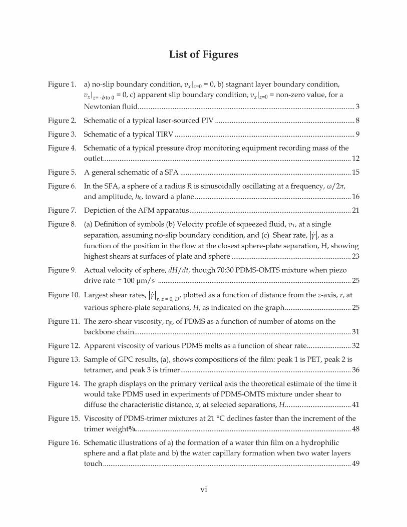
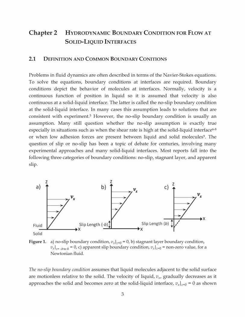
2.1 DEFINITION AND COMMON BOUNDARY CONITIONS Problems in fluid dynamics are often described in terms of the Navier-Stokes equations. To solve the equations, boundary conditions at interfaces are required. Boundary conditions depict the behavior of molecules at interfaces. Normally, velocity is a continuous function of position in liquid so it is assumed that velocity is also continuous at a solid-liquid interface. The latter is called the no-slip boundary condition at the solid-liquid interface. In many cases this assumption leads to solutions that are consistent with experiment.5 However, the no-slip boundary condition is usually an assumption. Many still question whether the no-slip assumption is exactly true especially in situations such as when the shear rate is high at the solid-liquid interface6-8 or when low adhesion forces are present between liquid and solid molecules9. The question of slip or no-slip has been a topic of debate for centuries, involving many experimental approaches and many solid-liquid interfaces. Most reports fall into the following three categories of boundary conditions: no-slip, stagnant layer, and apparent slip.

Figure 1. a) no-slip boundary condition, vx|z=0 = 0, b) stagnant layer boundary condition,

vx|z= -b to 0 = 0, c) apparent slip boundary condition, vx|z=0 = non-zero value, for a Newtonian fluid.

The no-slip boundary condition assumes that liquid molecules adjacent to the solid surface are motionless relative to the solid. The velocity of liquid, vx, gradually decreases as it approaches the solid and becomes zero at the solid-liquid interface, vx|z=0 = 0 as shown

4

(1)

schematically in Figure 1 a). The no-slip concept is dated back to 1738 when it was proposed by Bernoulli.10 This concept was supported by Stoke11, 12, Coulomb13, Warburg14 , and Couette15. The stagnant layer boundary condition assumes that there is a stationary liquid layer adsorbed onto a solid-liquid interface. Further into the liquid, the molecules have a finite velocity as shown in Figure 1 b). The model suggests that there is a discontinuity in the velocity within the body of liquid, which is not plausible because it violates the continuum of the Navier Stoke (N-S) equation, although the equation was not yet discovered when Girard proposed the stagnant layer model in 1813.16 From his flowing liquid through tubes experiments, Girard concluded that the liquid layer has a constant thickness if the solid material is consistent throughout, and this thickness is dependent upon types of solid and liquid, and temperature. He postulated that the thickness reduces to zero when the liquid is non-wetting, for example mercury on glass. Later, others17 proposed that a layer of air was introduced at an interface of non-wetting liquids; the problem becomes how liquid behaves at a gas-liquid interface rather than a solid-liquid interface and is beyond the scope of this thesis. The partial slip boundary condition assumes that the velocity of liquid molecules is not the same as that of the adjacent solid. The liquid molecules are said to be slipping at the velocity inversely proportional to the opposing frictional force exerted by the solid wall. In 1823, Navier introduced the concept of a slip length, b, which is proportional to a slip velocity in a Newtonian fluid:18

vx|z=0 = bvx

z . A slip length, b, is a distance from a solid-liquid interface to some point inside a solid where an extrapolated vx is zero as illustrated in Figure 1 c). A liquid velocity at a solid-liquid interface is represented by vx|z=0 . The experimental evidence of partial slip was found as early as in 1860 by Helmholtz and Piotrowski.19 2.2 HISTORY OF STUDY OF LIQUID FLOW AT INTERFACES In 1801, Coulomb13 conducted an experiment by submerging a vibrating metal disk in water. He repeated the experiment using tallow-coated disks and sandstone-coated disks. The adjacent liquid was found to move with the disk regardless of the coating;

5

(2)

these results support the no-slip boundary condition. Stokes11 performed a similar experiment when he was delegated by the Royal Academy of Science to investigate the nature of liquid at solid-liquid interfaces. From his oscillating cylinder experiment, he found that liquid molecules adjacent to the cylinder travel with it. He also found that the liquid velocity reduced with the distance into the bulk and reached a zero velocity at a few millimeters away from the cylinder. Stokes favored the no-slip boundary condition. On the other hand, Poiseuille20 never chose to express opinion on the boundary condition regardless of his numerous hydrodynamic experiments, perhaps due to inconsistent outcomes. His unique method, which paved ways for other scientists, was the study of the laminar flow of a Newtonian fluid inside a channel subject to a pressure difference p, along the channel. This was described in terms of Poiseuille’s law for Newtonian fluids,

Q = 2wh3

3p

L , of viscosity, , flowing through a channel of a width, w, a height, 2h, and a length, L at a flow rate, Q. Poiseuille showed that viscosity of water is a constant when flowed through tubes of vastly different radii. The results support no-slip boundary condition, which he used to arrive at equation (2). On the contrary, he reported observations of stagnant layers of blood on walls of the arteries and colloidal liquid on the solid-liquid interface inside glass tubes; both of which layers are thinner than the ones observed by Girard16. Using the Poiseuille flow, Warburg14 examined the flow of mercury through glass tubes and found no slipping. Couette15 also investigated flow through an assortment of small tubes made of glass, copper, white metal, and paraffin. He also coated the inner wall of some tubes with silver and grease to study the effect of hydrophobic coating. Flow rates were ramped up to the critical value where the flow became turbulent. Due to no change in efflux time between different types of tube and slightly faster time in coated tubes, in which he believed was a result of the smaller inner diameter, Couette concluded that liquid molecules near the solid-liquid interface did not slip even when the flow rate was high, and the flow was turbulent.

6

Nonetheless, there were those who believed that slip existed. Navier18 based his justification for slip on the molecular theory and proposed the quantifying method for slip length, b, as described in equation (1), which is still widely accepted presently. Piotrowski19 experimentally detected slip using his original oscillating sphere setup. The sphere is hollow, coated with grease on the inner wall and suspended with two wires on its axis. The cavity within the sphere was filled with a different liquid – water, ether, and alcohol – each time then torsionally oscillated about its vertical axis for viscosity measurement, where Pitrowski’s slip detection manifested. Helmholtz19 repeated Pitroski’s experiment utilizing metal sphere containing viscous liquids. His viscosity measurements were up to 40 percent higher than known values in which he thought was the result of slip length, b o a conscientious repetition of Pitrowski and Helmholtz’s experiment was carried out by Ladenburg21. He found no slip inside an oscillating hollow silver sphere filled with water and pinpointed the error in Helmholtz’s viscosity calculation. His recalculation of Helmholtz and Pitrowski’s data19 showed that the measured viscosity was in fact 3 percent higher than the known value, rather than 40 percent by previous evaluation, which fell within the margin of error and could not be accounted for an evidence of slip. For a long period of time thereafter, the no-slip boundary condition was generally accepted merely due to lack of strong evidences against it. It was agreed within the scientific community that if slip does exist, it can only be observed in very close vicinity to a solid-liquid interface. There was no equipment at the time that possessed such resolution. By the end of the 20th century, a number of tools have acquired micro- and nano-scale resolutions which allowed the boundary condition problems to be revisited. 2.3 CURRENT TECHNIQUES FOR EXAMINING FLOW AT INTERFACES At the turn of the last quarter of the 21st century, interest in the nanoworld has spawned development of an array of equipments with micro- and nano-scale resolution, and also the need for fluid handling on the micro- and nano-scale. Thus, there is the need to revisit the solid-liquid boundary condition to determine the flow in narrow channels with more precision. The impact of slip in microfluidic cannot be disregarded as in the macro scale as the influence of slip on the overall flow can be large. For instance, consider liquid of a viscosity, , and a density, , flowing through a pipe with a radius R

R = 10 cm both having the same length, L. While maintaining a constant liquid flow rate, Q, through the pipe, the pressure drop, , changes as a function of slip length, b:

7

(3)

p = 8 LQ

R41

1 + 4bR

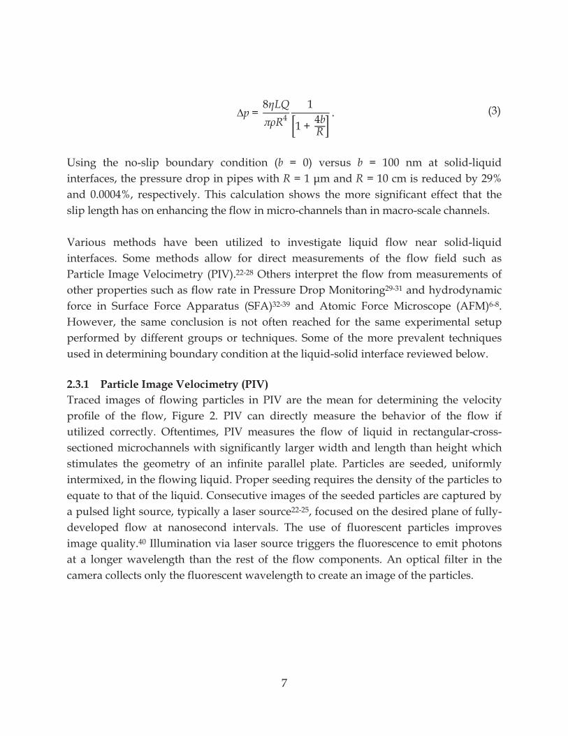
. Using the no-slip boundary condition (b = 0) versus b = 100 nm at solid-liquid interfaces, the pressure drop in pipes with R R = 10 cm is reduced by 29% and 0.0004%, respectively. This calculation shows the more significant effect that the slip length has on enhancing the flow in micro-channels than in macro-scale channels. Various methods have been utilized to investigate liquid flow near solid-liquid interfaces. Some methods allow for direct measurements of the flow field such as Particle Image Velocimetry (PIV).22-28 Others interpret the flow from measurements of other properties such as flow rate in Pressure Drop Monitoring29-31 and hydrodynamic force in Surface Force Apparatus (SFA)32-39 and Atomic Force Microscope (AFM)6-8. However, the same conclusion is not often reached for the same experimental setup performed by different groups or techniques. Some of the more prevalent techniques used in determining boundary condition at the liquid-solid interface reviewed below. 2.3.1 Particle Image Velocimetry (PIV) Traced images of flowing particles in PIV are the mean for determining the velocity profile of the flow, Figure 2. PIV can directly measure the behavior of the flow if utilized correctly. Oftentimes, PIV measures the flow of liquid in rectangular-cross-sectioned microchannels with significantly larger width and length than height which stimulates the geometry of an infinite parallel plate. Particles are seeded, uniformly intermixed, in the flowing liquid. Proper seeding requires the density of the particles to equate to that of the liquid. Consecutive images of the seeded particles are captured by a pulsed light source, typically a laser source22-25, focused on the desired plane of fully-developed flow at nanosecond intervals. The use of fluorescent particles improves image quality.40 Illumination via laser source triggers the fluorescence to emit photons at a longer wavelength than the rest of the flow components. An optical filter in the camera collects only the fluorescent wavelength to create an image of the particles.

8

Figure 2. Schematic of a typical laser-sourced PIV. Images of particles in a liquid of viscosity,

, at distance, H, from the solid-liquid interface are captured nanoseconds apart, at times t = 0 and t = t1. The flow pattern of the particles is analyzed by cross-correlation. [Neto, C.; Evans, D. R.; Bonaccurso, E.; Butt, H.-J.; Craig, V. S. J., Boundary slip in Newtonian liquids: a review of experimental studies. Reports on Progress in Physics 2005, (12), 2859.]41 (used under fair use guidelines, 2011)

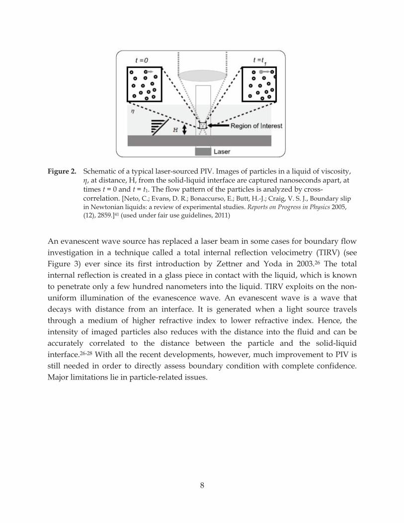
An evanescent wave source has replaced a laser beam in some cases for boundary flow investigation in a technique called a total internal reflection velocimetry (TIRV) (see Figure 3) ever since its first introduction by Zettner and Yoda in 2003.26 The total internal reflection is created in a glass piece in contact with the liquid, which is known to penetrate only a few hundred nanometers into the liquid. TIRV exploits on the non-uniform illumination of the evanescence wave. An evanescent wave is a wave that decays with distance from an interface. It is generated when a light source travels through a medium of higher refractive index to lower refractive index. Hence, the intensity of imaged particles also reduces with the distance into the fluid and can be accurately correlated to the distance between the particle and the solid-liquid interface.26-28 With all the recent developments, however, much improvement to PIV is still needed in order to directly assess boundary condition with complete confidence. Major limitations lie in particle-related issues.

9

Figure 3. Schematic of a typical TIRV. Evanescent wave source penetrates a small distance

above the solid-liquid interface. The particles scatter this light, and the intensity of scattering decays exponentially with distance from the interface. [Huang, P.; Breuer, K. S., Direct measurement of slip length in electrolyte solutions. Physics of Fluids 2007, 19, (2), 028104.]27 (used under fair use guidelines, 2011)

Typical particle sizes used in current PIV researches are on the order of hundreds of nanometers. These particles are large enough to emit adequate fluorescence for optical imaging and to reduce the amplitude of the Brownian motion. Nevertheless, the Brownian motion of small particles in liquid is inevitable. Cross-correlation analysis of consecutive images can largely account for the Brownian motion and give an accurate velocity profile of the liquid. Quantum dots grown on the surface of fluorescent particle is a prospective new technique that will reduce the particle size without sacrificing image resolution.42 There is also the concern that electrostatic and electro-kinetic forces introduced by double layers on both the particles and the solid will affect the results. A theory relating slip length to electrostatic properties of the system was proposed by Lauga43 which explained the cause of slip lengths in some experiments44 but disagreed with various other results22. In order to avoid erroneous results, a portion of the flow near surface has to be excluded from the analysis, which is the width of the double-layer that varies inversely with the salt concentration, e.g. 20-nm exclusion volume was reported for a slightly charged 10-5 M NaCl aqueous solution in contact with hydrophilic glass.25 In fact, the concentration of particles in the film of their diameter-sized thickness above the solid-liquid interface is so scarce that the flow in this region is estimated by extrapolation of the velocity.28 An additional source of error comes from inaccurate solid-liquid interface positioning in traditional PIV, i.e. excluding TIRV. At the bottom of the flow, some particles are assumed to be stuck to the wall, and that is where the solid-liquid interface is located; the technique was used in the latest report

10

with 30 nm confidence.24 Combining the fact that the particles themselves may be larger than the slip lengths, the presence of electrostatic forces, the need for velocity extrapolation, and the inaccurate solid-liquid interface positioning, errors in slip report from PIV can be substantial. One of the most discussed results is from the 2002 report by Tretheway and Meinhart.22 They observed pressure-driven, capillary flows of water seeded with polystyrene spheres, 300-nm diameter in size, over hydrophilic and octadecyltrichlorosilane- (OTS) coated hydrophobic glass surfaces. No slip was found at the hydrophilic glass surface.

from the last data point at 450- separation. In their later report23, slips were attributed to nanobubbles on the solid surface. Joseph and Tabeling24 took a very similar approach for slip investigation at shear rates of 20 – 500 s-1. They made sure that the surface of the test channel was smooth and reduced the particulate diameters to 100 nm. They found slips on the order of b 100 nm on both hydrophobic and hydrophilic surfaces, which are significantly smaller than the previous report22, 23. Instead of traditional PIV, groups like Yoda’s and Breuer’s chose to explore boundary condition at solid-liquid interface with TIRV. Huang and Breuer27 conducted the experiment using ionic solution and water seeded with 100-200 nm diameter spheres at shear rates between 200-1900 s-1. How they accounted for the decay in image resolution in the cross-correlation analysis was unclear. Slips in the same order of magnitude, 100 nm, were found in both ionic and non-ionic systems, which led them to believe that ionization does not affect slip at the solid-liquid interface. The effect of shear rate on slip was also not found, although they commented that it was premature to conclude so due to shear rates having only an order of magnitude difference. Li and Yoda28 also observed Poiseuille flow of both seeded ionic solution and water. Their report showed that ionization increases the particle concentration 100 nm, the nominal diameter of particles, above solid-liquid interface. Below 100 nm, however, particle concentration rapidly dropped to nearly nonexistent. More accurate analysis of particle velocity was attained by dividing the liquid into 3 layers – I, II and II – according to the distance above the solid-liquid interface, layer I being adjacent to the solid-liquid interface. They stated that the evanescent-wave technique only measures the true velocity of layer II that is most in-focus. It overestimates the velocity of particles in layer I and underestimates that of layer III, which if not accounted for would result in a false slip observation. Particles in layer I underwent asymmetric diffusion due to no-flux boundary condition, which was negligible in this specific case. Nonetheless, the out-of-focus particles in layer III required corrections via the particle-tracking method45 to

11

(4)

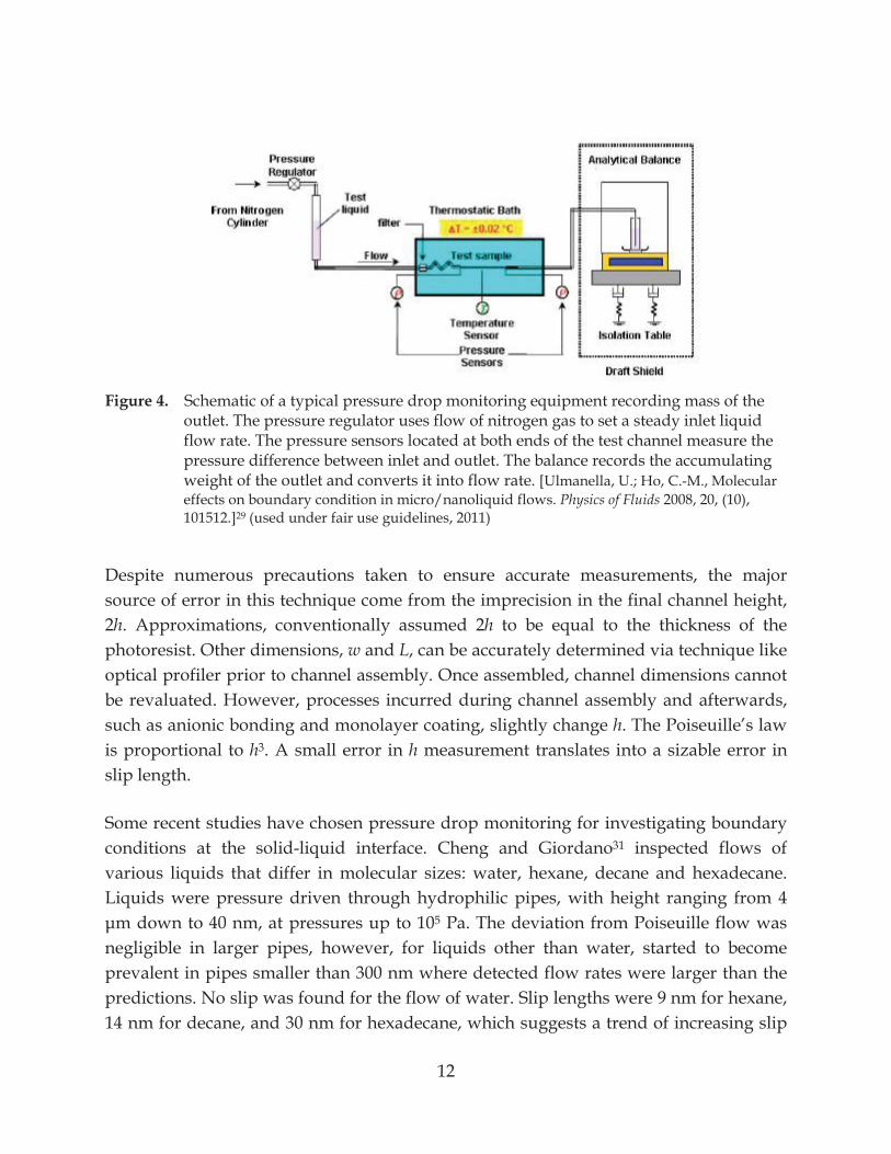
deduce accurate velocity estimations. As a result, the particle velocity in both ionic and water extrapolated to zero at the solid-liquid interface, in other word, no slip. So far, reviewed studies have been those of pressure-driven fluid motion. Alternatively, Joly et al25 chose to propel their seeded fluids in a confined geometry by thermal agitation. By doing so, they claim to have eliminated the nanobubble formation at the solid-liquid interface caused by shear stress, which is present in pressure-driven flows. The fluid is agitated by an argon laser source, and diffusion coefficients of the florescent particles near the solid-liquid interface are measured. Coefficients of diffusion of particles adjacent to hydrophilic surface overlay with the predicted values assuming no-slip boundary condition. Adjacent to the hydrophobic surface, particles were found to diffuse faster than expected, corresponding to 18±5 nm slip length, which is agreeable with previously reported SFA results36. 2.3.2 Pressure Drop Monitoring The Poiseuille’s law (equation (2)) governing the flow in a rectilinear channel assumes no-slip boundary condition and predicts the outlet flow rate, Q, given known channel dimensions – width, w, height, 2h, and length, L – an p. If all the parameters in equation (2) are measured, then the assumption of the no-slip boundary can be tested. The apparatus for pressure drop monitoring is illustrated schematically in Figure 4. Departure from the Poiseuille’s law is accounted for by additional flow due to slip, Qslip:30

Q = 2wh3

3p

L + Qslip= 2wh3

3p

L + 2hw vx|z=0 , where vx|z=0 is the liquid velocity at the solid-liquid interface. The equipment conventionally consists of two solid substrates; one contains a photoresist that has been fabricated by some lithographic technique into desired dimensions, another is a piece of glass covered by a photoresist. A topographic technique like AFM is used to examine the smoothness of surfaces, then the two substrates are assembled into a channel by either anodic bonding30, 31 or screws systems29. Fabrication of hydrophobic channels requires an additional step of self-assembled monolayer (SAM) coating.30 Liquids are pushed through a filter then through to the channels by a controllable microsyringe pump. Pressure monitors are installed on both ends of the channel to record inlet and outlet pressures, i.e. pressure drop. The flow outlet can be recorded in terms of weight or volume. Liquid evaporation is preventable by applying a layer of silicone oil on top of liquid in the reservoirs.29

12

Figure 4. Schematic of a typical pressure drop monitoring equipment recording mass of the

outlet. The pressure regulator uses flow of nitrogen gas to set a steady inlet liquid flow rate. The pressure sensors located at both ends of the test channel measure the pressure difference between inlet and outlet. The balance records the accumulating weight of the outlet and converts it into flow rate. [Ulmanella, U.; Ho, C.-M., Molecular effects on boundary condition in micro/nanoliquid flows. Physics of Fluids 2008, 20, (10), 101512.]29 (used under fair use guidelines, 2011)

Despite numerous precautions taken to ensure accurate measurements, the major source of error in this technique come from the imprecision in the final channel height, 2h. Approximations, conventionally assumed 2h to be equal to the thickness of the photoresist. Other dimensions, w and L, can be accurately determined via technique like optical profiler prior to channel assembly. Once assembled, channel dimensions cannot be revaluated. However, processes incurred during channel assembly and afterwards, such as anionic bonding and monolayer coating, slightly change h. The Poiseuille’s law is proportional to h3. A small error in h measurement translates into a sizable error in slip length. Some recent studies have chosen pressure drop monitoring for investigating boundary conditions at the solid-liquid interface. Cheng and Giordano31 inspected flows of various liquids that differ in molecular sizes: water, hexane, decane and hexadecane. Liquids were pressure driven through hydrophilic pipes, with height ranging from 4

5 Pa. The deviation from Poiseuille flow was negligible in larger pipes, however, for liquids other than water, started to become prevalent in pipes smaller than 300 nm where detected flow rates were larger than the predictions. No slip was found for the flow of water. Slip lengths were 9 nm for hexane, 14 nm for decane, and 30 nm for hexadecane, which suggests a trend of increasing slip

13

length with increasing molecular size. On the other hand, Choi et al30 chose to focus solely on the flow of water through two channel sizes, h = 0.5 h = 1 Interestingly, they also hydrophobized some of the channels and were able to show the hydrophobic meniscus formation of evaporating water within the pipe as to verify the property. Water was pushed through the channels at shear rates up to 105 s-1. Slip lengths were found on hydrophilic surfaces and even larger on hydrophobic surfaces. They thought that slip measured on hydrophilic surfaces was artificial and suggested that they arose from discrepancies in the channel height measurement. After making the correction to the channel height to fit the data on hydrophilic surfaces to illustrate no slip, they reanalyzed the data on hydrophobic surfaces. The reanalyzed data showed that slip on hydrophobic surfaces is an increasing function of shear rate up to 30 nm for a shear rate of 105 s-1. Ulmanella and Ho29 investigated the effect of polarity of the liquid on the boundary condition in hydrophilic channels, heights ranging from 350 nm to 5

For comparisons, isopropanol (dipole moment = 1.66 D) and non-polar n-hexadecane were pushed through the channels at shear rates up to 4×105 s-1. The results showed that n-hexadecane exhibited larger slip lengths (b = 0 - 40 nm) than isopropanol (b = 40 - 120 nm) as to conclude that the lack of polarity can introduce slip at the solid-liquid interface. Slip lengths were found to increase with the shear rate although unaffected by the channel height. In all above cases, researchers studied the nature of the boundary condition at conventional solid-liquid interfaces. Let us now be introduced to others who had intentionally modified the interface to change the solid-liquid boundary condition. Superhydrophobic surfaces are the subject of much recent research and are one of the ways to introduce slip at the solid-liquid interface. In a series of papers, Ou et al46, 47 reported evidence of water slipping at superhydrophobic surfaces. Such surfaces were achieved by fabrication of microposts on the surface. Lithography permitted a precise control of the pole size and their coverage. During the flow, water only made contact with the top of these microposts without touching the floor. Gaps between microposts were filled with air. Therefore, less solid-liquid contact led to more drag reduction and larger slip length. They were able to achieve up to 40% pressure drop reduction and 21-

- – 25 mm3/s. On the other approach, Majumder and co-workers48 exploited on the hydrophobic properties of carbon nanotubes. They drove water and various other solvents through 7-nm diameter nanotubes, produced in-house. The weak interaction between carbon and water molecules is expected to drive the formation of ordered hydrogen bonds

14

(5)

(6)

between water molecules, which are conducive to faster flow. The water flow rate through nanotubes was 5 orders of magnitudes higher than that predicted for no-slip flow. At this rate, the flow is comparable to the frictionless flow in biological channels. As for other solvents – ethanol, iso-propanol, hexane and decane – the flow rate decreased with the affinity to the carbon nanotube walls. Nonetheless, the flow rate was still found to be 3 orders of magnitude higher than expected for decane. 2.3.3 Surface Force Apparatus (SFA) In 1972, Israelachvili32 devised the first surface force apparatus (SFA) to measure forces in fluids confined between two surfaces. The surfaces are crossed cylinders of equal radius, R, separated by a distance, H.32-35 The curvature of the crossed cylinders geometry emulates a sphere-plane geometry, commonly used in atomic force microscopy (AFM) as well as in recent SFA experiments36-39. Assuming (a) separations are much less than the radius, H R, and (b) the no-slip boundary condition applies at solid-liquid interfaces, the lubrication force, FL, between a sphere and a plane is expressed by the Reynolds equation:49

FL = - 6 R2 v1H ,

where is the viscosity of the fluid, and v is the velocity of a sphere (AFM) or a cylinder (SFA). If slip of b on each surface were to occur, then Vinogradova showed that equation (5) is modified by factor of f* as follows:9

FL = - 6 R2 v × 1H f*; f* =

14 1 + 3H2b 1+

H4b ln 1+

4bH - 1 .

At large separations, H >> b, this is equivalent to replacing H in equation (6) by H + 2b, i.e. effectively the sphere and plate surfaces are each shifted further apart by a distance b. Note that the SFA directly senses the lubrication force as a function of H, whereas slip length are measured indirectly by comparing to the theory of the force, equation (6). A schematic of a typical SFA is illustrated in Figure 5. The separation, H, between two surfaces is precisely controlled by the piezoelectric crystal. For most experiments, one surface is held fixed while the other sinusoidally oscillates at a frequency, /2 , and an amplitude, h0, toward the fixed surface by expanding and contracting motions of the crystal (Figure 6). The motion is detected by a multiple beam interferometer with a ± 0.1 nm precision.50 The velocity of the moving surface, , is the product of its angular velocity and amplitude, 0. Radii of the surfaces are in the millimeter range, which

15

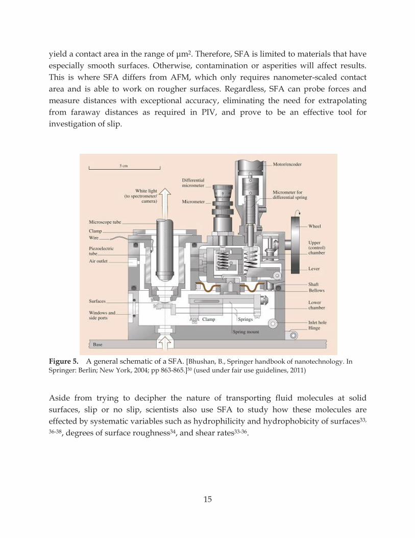
2. Therefore, SFA is limited to materials that have especially smooth surfaces. Otherwise, contamination or asperities will affect results. This is where SFA differs from AFM, which only requires nanometer-scaled contact area and is able to work on rougher surfaces. Regardless, SFA can probe forces and measure distances with exceptional accuracy, eliminating the need for extrapolating from faraway distances as required in PIV, and prove to be an effective tool for investigation of slip.

Figure 5. A general schematic of a SFA. [Bhushan, B., Springer handbook of nanotechnology. In Springer: Berlin; New York, 2004; pp 863-865.]50 (used under fair use guidelines, 2011)

Aside from trying to decipher the nature of transporting fluid molecules at solid surfaces, slip or no slip, scientists also use SFA to study how these molecules are effected by systematic variables such as hydrophilicity and hydrophobicity of surfaces33,

36-38, degrees of surface roughness34, and shear rates33-36.

16

Figure 6. In the SFA, a sphere of a radius R is sinusoidally oscillating at a frequency, /2 ,

and amplitude, h0, toward a plane. The inset shows sphere-plane separation, H, as a function of time, t. The velocity profile indicates an asymmetric system where no-slip boundary condition applies at the surface of sphere but not above plane, i.e. hydrophilic sphere and hydrophobic plane. [Cottin-Bizonne, C.; Steinberger, A.; Cross, B.; Raccurt, O.; Charlaix, E., Nanohydrodynamics: The Intrinsic Flow Boundary Condition on Smooth Surfaces. Langmuir 2008, 24, (4), 1165-1172.]38 (used under fair use guidelines, 2011)

The effect of hydrophilicity and hydrophobicity of surfaces on slip is typically quantified by varying the solid coating and the type of liquid to obtain a range of desired contact angles from small to large. Zhu and Granick33 reported having found unusually large slip lengths of water at surfaces hydrophobized with octadecyltriethoxysiloxane (OTE). They also found that slip length increases with both contact angles and shear rates. The unusually large slip lengths were thought to be caused by vibration-induced nanobubbles at solid surfaces. It was later realized that their surfaces could have been contaminated by platinum nanoparticles during the preparation of mica.51 These particles are pinpointed as the cause for shear dependency of the slip length. Nanoparticles are a form of surface roughness, which reportedly reduces slip, at low shear rates.34 At higher shear, these particles are expected to nucleate nanobubbles and increase slip.52 Zhu and Granick corrected the slip-length value of water at OTE-coated surfaces to 36 nm in their 2002 report.34 To interpret their result, there are two identical surfaces in the SFA setup so the slip on each surface should only be half of the reported vale, b Nonetheless, shear dependency of the slip length was still found. Here they also studied the effect of nanometer-scaled roughness on the slip length and proposed maximum shear rates required to observe slip as a function of surface roughness. The nanometer-scaled roughness enhances the no-slip boundary condition. Unlike the macro-scaled roughness, the nanometer-scaled features do no trap air between them. Instead, they make it harder for liquid molecules to slip off the surface. Surfaces with a root-mean-square (rms) roughness of 6 nm

17

exhibited no slip at solid-liquid interfaces under high shear up to 105 s-1. On the other side of the spectrum, atomically smooth hydrophobic surfaces, rms roughness 0.2 nm, exhibit slip at shear rates over 102 s-1. Baudry and Charlaix36 also attempted to find the correlation between slip length and surface hydrophobicity, using sphere-plane geometry submerged in glycerol, instead of crossed-cylindrical geometry. The speed of the sphere oscillating toward the plane never exceeded 0.5 nm/s. At this rate, no evidence of slip was found on hydrophilic cobalt surfaces, and a slip length of 38 nm was reported on hydrophobic surfaces. Unlike previous reports, the reported slip length did not vary with the shear rate. Bizonne et al37, 38 also utilized the sphere-plane geometry in their SFA. Interestingly, they created an asymmetric system by only modifying just the plane and leaving all spheres hydrophilic creating a velocity profile as shown in Figure 6. As no-slip boundary is likely to hold at the hydrophilic surface22, 25, 28, 30, 31 of the sphere, any detectable slip would have to occur on the plane. Contact angles achieved on the plane were 3° (unmodified), 28°, 95°, and 105°. The effect of shear rate on slip was successfully mitigated by keeping the shear rates below 5×103 s-1. No slip boundary condition applied to hydrophilic and partially-wetting surfaces, contact angles 3° and 28°, respectively. For hydrophobic surfaces, slip length increases with the contact angle with a maximum b 19 nm; this result is comparable to the slip length quantified by a shear free method25 which led them to conclude that the slip length is intrinsic to hydrophobic surfaces. In addition, Steinberger et al39 made the claim via numerical stimulation that slip is a controllable factor via controlling features on superhydrophobic surfaces. Typical superhydrophobic surfaces are assumed to reduce fluid drag by introducing air traps at solid-liquid interfaces. The air trap has a meniscus shape (meniscus angle, ) that depends upon the size and the spacing of features on superhydrophobic surfaces. The stimulation predicts slip lengths from these meniscus angles. From the prediction, slip lengths from -280 nm to 200 nm, including 0 slip, can theoretically be attained. Experimentally, however, much further investigations are still necessary. Steinberger and his coworkers only compared 2 surfaces, with and without air traps between surface features, respectively Wenzel regime and Cassie regime. They found a larger slip length, b 105 nm, on the Wenzel regime than on the Cassie regime, b 20 nm, using a sphere-plate SFA and a mixture of water and glycerol = 39 mPa s; the intent was to show that a lower degree of slip can be achieved with a hydrophobic surface than a hydrophilic surface. However, the reliability of this report is questionable. Locating a solid-liquid interface on a hydrophilic surface containing features

18

(roughness) could be a difficult task and may have been the source of such large reported slip length. Lastly, and possibly the most relevant to this thesis, the boundary condition of polymer solution at hydrophilic mica surfaces was studied in Horn et al35 via a crossed cylinders SFA. Slip boundary condition (b = 30 – 50 nm) was found for films thicker than 70 nm under shear rates of 1 – 1000 s-1. Slip lengths increased with higher shear rates and thinner films. Some similarities to the work in this thesis include (a) the polymer solution was a Boger fluid, i.e. its bulk properties are shear-independent, (b) the melt consists of both distinctly short- and long-chained polymers, and (c) the long-chained polymers have high polydispersity (PDI (a) their polymers were diluted in kerosene whereas polymers used in this thesis were a pure melt at room temperature, (b) their solution consisted of only 0.1% long-chained polymer versus the homopolymer melt used in this thesis that contained 70% of the long-chained polymer, (c) their maximum shear rates are an order of magnitude lower than the rates used in this thesis, and (d) their surfaces were hydrophilic versus hydrophobic surfaces used in this thesis for the same purpose. From a theoretical point of view, the two-layer model, equation (9), predicted the effect of decrease in segment density near their solid-liquid interface to have caused a slip length of 2.2 nm, which is still too little to account for the measured slip. The two-layer model could have been too simple for this prediction because it does not account for the gradual decrease in the viscosity. From the experiment, they found that the effects of van der Waals force and depletion force were too small to account for the deviation of the measured force from the hydrodynamic prediction via equation (5), hence the intrinsic effect of the polymer solution was considered. Boger fluids under shear are known to decrease in segment density, i.e. viscosity, from bulk value to zero at a liquid-solid interface;35 by this logic, the thin layer adjacent to the solid should have the low viscosity of the solvent. The increase of slip length with shear rate suggests that there is a polymer depletion layer at the solid-liquid interface, and shear-induced migration away from the solid seems to be the most sounding conclusion. 2.3.4 Results Summary Results from this chapter are summarized in Table 1. Most of the results are agreeable upon one thing: there is no slip at hydrophilic surfaces.22, 25, 28, 30, 36-38 Increased contact angles tend to increase slip length.22, 25, 27, 33, 36-38 Slip was found at smooth hydrophobic surfaces (contact angle > 95°), and multiple reports25, 34, 37, 38 agreed upon b being intrinsic to such surface. Nano-scale roughness on hydrophobic surfaces was found to promote no-slip boundary condition,34 whereas micro-scale roughness

19

(7)

(8)

(9)

increases slip length46, 47 by enabling air to be trapped between features, which reduces interfacial drag by minimizing solid-liquid contact. The slip length increased with shear rates in some experiments. For polymer solutions, variation of slip measurement with shear may be caused by a depletion layer.35 Slip was also found to increase with molecular size.31 Other causes considered for slip are (a) nanobubble formation22 at the solid-liquid interface and (b) thin layer of a different liquid35 existing between the solid and the bulk liquid. The nanobubble theory, equation (7), states that, for a rarified gas in contact with liquid, slip length is a function of an air gap thickness, , a surface fraction covered with bubbles, f, and a separation between solids, H.

b = 2f l + 2

2 + + H

a(2 – f )H ,

where l and a are viscosities of liquid and air (8) below:

urare|z = - = dudz

z = -.

Equation (8) is the boundary condition describing the velocity of rarified gas, urare, at the liquid-gas interface (z = - ). The two-layer theory states that a thin film of low viscosity fluid at an interface between a solid and a bulk liquid is expected to reduce shear stress at an interface, thereby causing a decrease in the lubrication force. Vinogradova9 provides the estimate of order of the equivalent slip length that results from such thin film:

1f

b b ,

where is the thickness of the film, b is the viscosity of the bulk liquid and f is the viscosity of the liquid in the thin film.

20

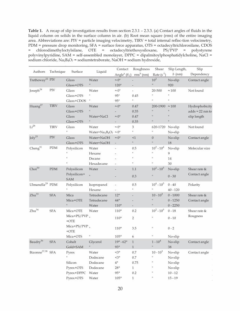
Table 1. A recap of slip investigation results from section 2.3.1 – 2.3.3. (a) Contact angles of fluids in the liquid column on solids in the surface column in air. (b) Root mean square (rms) of the entire imaging area. Abbreviations are: PIV = particle imaging velocimetry, TIRV = total internal reflec-tion velocimetry, PDM = pressure drop monitoring, SFA = surface force apparatus, OTS = octadecyltrichlorosilane, CDOS = chlorodimethyloctylsilane, OTE = octadecyltriethoxysiloxane, PS/PVP = polystyrene polyvinylpyridine, SAM = self-assembled monolayer, DPPC = dipalmitoylphosphatidylcholine, NaCl = sodium chloride, Na2B4O7 = sodiumtetraborate, NaOH = sodium hydroxide,

Contact Roughness Shear Slip Length, Slip

Anglea ( C) rmsb (nm) Rate (s-1) b (nm) Dependency

Tretheway22 PIV Glass Water - 102 No-slip Contact angleGlass+OTS ” - ” 920

Joseph24 PIV Glass Water - 20-500 Not foundGlass+OTS " 0.45 " "Glass+CDOS " " " "

Huang27 TIRV Glass Water 0.47 200-1900 HydrophobicityGlass+OTS " - 0.35 " "Glass Water+NaCl 0.47 " " slip lengthGlass+OTS " - 0.35 " "

Li28 TIRV Glass Water 3 620-1720 No-slip Not found" Water+Na2B4O7 " " No-slip

Joly25 PIV Glass Water+NaOH <1 0 No-slip Contact angleGlass+OTS Water+NaOH - " " 18

Cheng31 PDM Polysilicon Water - 0.5 102 - 104 No-slip Molecular size" Hexane - " " 9" Decane - " " 14" Hexadecane - " " 30

Choi30 PDM Polysilicon Water - 1.1 102 - 105 No-slip Shear rate &Polysilicon+ Contact angleSAM

Ulmanella29 PDM Polysilicon Isopropanol - 0.5 104 - 105 0 - 40 Polarity" Hexane - " " 40 - 120

Zhu33 SFA Mica Tetradecane 12° - 10 - 105 0 - 1000 Shear rate &Mica+OTE Tetradecane 44° - " 0 - 1250 Contact angle" Water 110° - " 0 - 2250

Zhu34 SFA Mica+OTE Water 110° 0.2 102 - 105 0 - 18 Shear rate &Mica+PS/PVP Rougness+OTEMica+PS/PVP+OTEMica+OTS " 105° 6 " No-slip

Baudry36 SFA Cobalt Glycerol 19° - 62° 1 1 - 104 No-slip Contact angleGold+SAM " 93° 1 " 38

Bizonne37,38 SFA Pyrex Water <3° 0.7 10 - 103 No-slip Contact angle" Dodecane <3° 0.7 " No-slipSilicon Dodecane 4° 0.75 " No-slipPyrex+OTS Dodecane 28° 1 " No-slipPyrex+DPPC Water 95° 0.2 " 10 - 12Pyrex+OTS Water 105° 1 " 15 - 19

"

0 - 10

0 - 2

"

"

110° 2

3.5110°

- 0.3 " 0 - 30

"

Authors Technique Surface Liquid

"

21

Chapter 3 ATOMIC FORCE MICROSCOPY (AFM) Most scientific tools do not serve more than one purpose, but AFM is one that does. AFM originally served as a tool for imaging nanotopography of non-conducting materials that could not be probed via scanning tunneling microscopy (STM). For imaging, AFM utilizes a cantilever with a sharp nanometer-scaled tip. A tip is in contact with a surface and is scanned back and forth across an imaging area. A solid causes a force to act on a tip which causes a cantilever to deflect in response to topography of the solid surface. The photodiode determines deflections of a cantilever by monitoring the reflection of a laser from the end of a cantilever. The two imaging modes are (a) contact mode, where a tip is kept in contact with a surface at all times, and (b) tapping mode, where a cantilever oscillates near its resonant frequency to minimize friction and, thus, wear of soft or fragile materials.

Figure 7. Depiction of the AFM apparatus. As piezoelectric stage moves downward, the

lubrication force within the thin film of liquid counteracts the motion of the sphere and deflects the cantilever upwards. The velocity of the sphere is not equal to the piezo displacement rate due to deflection.

Imaging was the function of AFM until 1991 when Ducker et al53 made it into a surface force sensing machine. They attached a microscopic sphere to the free end of a cantilever and as a result achieved sphere-plane geometry (Figure 7) which is equivalent to the cross cylinders used in SFA. Therefore, theoretical lubrication force approximations using equations (5) and (6) are also valid for AFM. The lubrication force is measured when a sphere is moved through a fluid towards a flat surface. Such motion is achieved by expansion or contraction of a piezoelectric crystal in an AFM stage. The motion of a piezoelectric crystal is measured using a linear variable differential transducer (LVDT) or capacitance gauge. The fluid exerts forces against this motion of the sphere which causes the cantilever to deflect some distance, depending on

22

a spring constant, k, of the cantilever, so a higher k is required for viscous fluid like a PDMS. The amount of forces exerted by liquid is simply k times deflection. The one downside of AFM is due to indirect measurement of the separation; it is calibrated by assuming, while in contact with the plane, the displacements of piezo stage and cantilever deflection are the same. The sum of the piezo displacement and the deflection is the sphere-plate separation, H. At some point, this sum becomes a constant, which is where zero separation is assigned. The indirect measurement of the separation results in poorer resolution than that of SFA, 2-3 nm vs 0.1 nm, Regardless of the indirect separation measurement, the resolution of AFM is superior to most other methods used in slip investigation. It is able to utilize rougher samples and larger shear rates than SFA can. Only a small amount of sample is required. Experiments can be conducted under controlled environments in a closed fluid cell. For experiments described in this thesis, it is particularly useful to be able to use an AFM for roughness and force probing simultaneously to reduce surface contamination and degradation. Surface force measurements are based on theories presented in the next section. 3.1 THEORY 3.1.1 Velocity Profile and Shear Rate Brenner54 derived an exact solution to the lubrication force for a sphere moving towards a flat plate in a Newtonian liquid under creeping flow (Reynolds number Re << 1), which is in the limit of H << R and is given by equation (5):

FL = - 6 R2 v1H .

In a typical AFM experiment, Re = / . Assuming that the characteristic length, L, is the separation between the sphere and the plate. For a separation of 100 nm, velocity of

/s and liquid density, , of 970 kg/m3 (the maximum v and used in this thesis), Re is 1.2 × 10-8 for fluid of = 1000 mPa s and is 1.2 × 10-5 for that of = 1 mPa s. This satisfies the condition for Re << 1 in a typical AFM experiment. Chan and Horn49 utilized the lubrication approximation, which is valid in the region where H << R, to simplify Brenner’s velocity profile of the sphere-plane geometry.

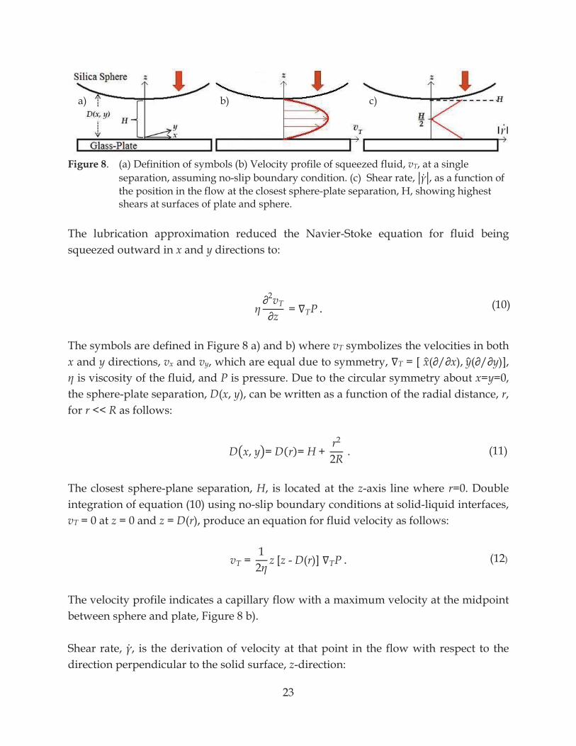
23

(10)

(11)

(12)

Figure 8. (a) Definition of symbols (b) Velocity profile of squeezed fluid, vT, at a single

separation, assuming no-slip boundary condition. (c) Shear rate, , as a function of the position in the flow at the closest sphere-plate separation, H, showing highest shears at surfaces of plate and sphere.

The lubrication approximation reduced the Navier-Stoke equation for fluid being squeezed outward in x and y directions to:

2vT = TP .

The symbols are defined in Figure 8 a) and b) where vT symbolizes the velocities in both x and y directions, vx and vy, which are equal due to symmetry, T = [ x( / ), y( / )],

is viscosity of the fluid, and P is pressure. Due to the circular symmetry about x=y=0, the sphere-plate separation, D(x, y), can be written as a function of the radial distance, r, for r << R as follows: D x, y = D(r)= H +

r2

2R . The closest sphere-plane separation, H, is located at the z-axis line where r=0. Double integration of equation (10) using no-slip boundary conditions at solid-liquid interfaces, vT = 0 at z = 0 and z = D(r), produce an equation for fluid velocity as follows:

vT = 1

2 z [z - D(r)] TP .

The velocity profile indicates a capillary flow with a maximum velocity at the midpoint between sphere and plate, Figure 8 b). Shear rate, , is the derivation of velocity at that point in the flow with respect to the direction perpendicular to the solid surface, z-direction:

a) b) c)

24

(13)

(14)

(15)

(16)

= vT(r, z)

= -3r

D3(r)[2z - D(r)] dH

dt , where dH/dt is the rate of change in sphere-plate separation , i.e. the velocity of sphere, which is set to a constant by linear expansion of the piezoelectric crystal. The largest shear rates occur at solid-liquid interfaces (where z = 0 and z = D(r)) (see Figure 8 c)). The expression for shear rates at solid-liquid interfaces is as follows:

r, z = 0, D=

vT(r, z = 0, D)=

3r(H + r2/2R)2

dHdt .

The maximum shear rate,

max, theoretically occurs at r = (2RH/3)1/2, which simplifies

equation (14) to:

max=

vT

max=

12

32

5/2 R1/2

H3/2 dHdt .

The maximum shear stress, max, caused by this maximum shear rate is the product of fluid viscosity, , and the maximum shear rate:

max= max

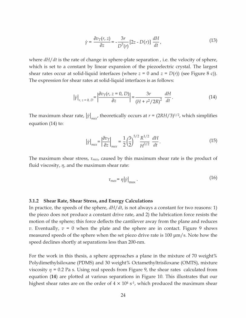
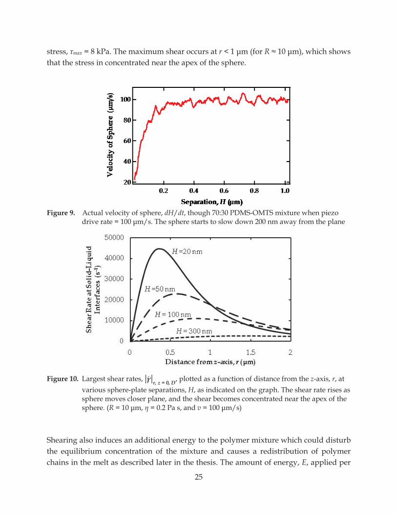
. 3.1.2 Shear Rate, Shear Stress, and Energy Calculations In practice, the speeds of the sphere, dH/dt, is not always a constant for two reasons: 1) the piezo does not produce a constant drive rate, and 2) the lubrication force resists the motion of the sphere; this force deflects the cantilever away from the plane and reduces v. Eventually, v = 0 when the plate and the sphere are in contact. Figure 9 shows measured speeds of the sphere when the set piezo ote how the speed declines shortly at separations less than 200-nm. For the work in this thesis, a sphere approaches a plane in the mixture of 70 weight% Polydimethylsiloxane (PDMS) and 30 weight% Octamethyltrisiloxane (OMTS), mixture viscosity = 0.2 Pa s. Using real speeds from Figure 9, the shear rates calculated from equation (14) are plotted at various separations in Figure 10. This illustrates that our highest shear rates are on the order of 4 × 104 s-1, which produced the maximum shear

25

stress, max = 8 kPa. The maximum shear occurs at r < R sthat the stress in concentrated near the apex of the sphere.

Figure 9. Actual velocity of sphere, dH/dt, though 70:30 PDMS-OMTS mixture when piezo

m/s. The sphere starts to slow down 200 nm away from the plane

Figure 10. Largest shear rates, r, z = 0, D, plotted as a function of distance from the z-axis, r, at various sphere-plate separations, H, as indicated on the graph. The shear rate rises as sphere moves closer plane, and the shear becomes concentrated near the apex of the sphere. (R = 0.2 Pa s, and v

Shearing also induces an additional energy to the polymer mixture which could disturb the equilibrium concentration of the mixture and causes a redistribution of polymer chains in the melt as described later in the thesis. The amount of energy, E, applied per

26

mole of PDMS molecule (mean radius of gyration, Rg = 3.6 × 10-9 m) in the mixture at the maximum shear rate is roughly the product of the maximum shear rate, a surface area of a PDMS molecule, and the diffusion distance at 20-nm separation where the maximum shear rate occurs, x|H=20nm ~ 400 nm (see Figure 10): E = maxRg2x = 25 kJ/mole PDMS. From Figure 10, it is obvious that the shear rate, hence shear stress, decreases with increasing diffusion distances beyond the point where max occurs. What is not obvious is that E remains quite the same at these distances because. For example at H = 20 nm, E = 25 kJ/mole PDMS at x = 800 nm where the shear stress is 50% of max and E = 23 kJ/mole PDMS at x = 1500 nm where the shear stress is 25% of max. However, shear stress and energy decrease with increasing separations regardless of x.

3.2 PRIOR AFM RESULTS Many early reports of slip lengths in Newtonian liquids via AFM force measurements reported large slip lengths.6, 7 Craig et al6 reported slip length up to ~20 nm at the solid-liquid interface between hydrophobic surfaces and aqueous sucrose solutions. The slip length increased with shear rate. However, they neglected a possible roughness contribution to slip since there was a 30° difference between advancing and receding contact angles of water on their hydrophobic surfaces. Neto et al7 conducted studies under similar conditions to those in Craig et al6 and found further evidence to support dependency of slip on shear rate and fluid viscosity. They found slip length up to ~185 nm in PDMS melt, = 99 mPa s. Such high slip could be an evidence chain migration of long PDMS chains away from the high shear field at close separations, although more detail on polymer properties are needed to say that conclusively. These early studies are probably not reliable. They were affected by (a) use of rough particles, where the roughness was not adequately incorporated into the physical model for the theoretical force, (b) incorrect calibration of the cantilever deflection sensor in the AFM, and (c) incorrect calibration of the spring constant.55 Later studies in nearly identical liquids reported contrasting results with no slips. Honig and Ducker described results that were consistent with the no-slip boundary condition at smooth solid-liquid interfaces: (a) aqueous sucrose solution at hydrophilic glass surface,56 and (b) PDMS melt at hydrophobic glass surface.8 As for hydrophilic surfaces in contact with PDMS melt, inconsistent slip lengths were detected and thought to be caused by a thin layer of water located between PDMS and glass based on the two-layer theory (equation (9)). No correlation was found between slip length and

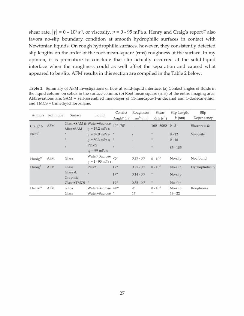
27

shear rate, = 0 – 105 s-1, or viscosity, = 0 - 95 mPa s. Henry and Craig’s report57 also favors no-slip boundary condition at smooth hydrophilic surfaces in contact with Newtonian liquids. On rough hydrophilic surfaces, however, they consistently detected slip lengths on the order of the root-mean-square (rms) roughness of the surface. In my opinion, it is premature to conclude that slip actually occurred at the solid-liquid interface when the roughness could as well offset the separation and caused what appeared to be slip. AFM results in this section are compiled in the Table 2 below.

Table 2. Summary of AFM investigations of flow at solid-liquid interface. (a) Contact angles of fluids in the liquid column on solids in the surface column. (b) Root mean square (rms) of the entire imaging area. Abbreviations are: SAM = self-assembled monolayer of 11-mercapto-1-undecanol and 1-dodecanethiol, and TMCS = trimethylchlorosilane.

Contact Roughness Shear Slip Length, Slip

Anglea ( C) rmsb (nm) Rate (s-1) b (nm) Dependency

Glass+SAM & Water+SucroseMica+SAM = 19.2 mPa s

Neto7 " = 38.9 mPa s " - " 0 - 12 Viscosity" = 80.3 mPa s " - " 0 - 18

PDMS = 99 mPa s

Water+Sucrose = 1 - 90 mPa s

Honig8 AFM Glass PDMS 17° 0.25 - 0.7 0 - 105 No-slip HydrophobicityGlass &GraphiteGlass+TMCS " 19° 0.35 - 0.7 " No-slip

Henry57 AFM Silica Water+Sucrose <1 0 - 104 No-slip RoughnessGlass Water+Sucrose " 17 " 13 - 22

0 - 105 No-slip Not found

" 17° 0.14 - 0.7 " No-slip

" " - " 85 - 185

Honig56 AFM Glass <5° 0.25 - 0.7

Shear rate &

Authors Technique Surface Liquid

40° - 70° - 160 - 8000AFMCraig6 & 0 - 5

28

Chapter 4 REVIEW OF POLYDIMETHYLSILOXANE (PDMS)

PROPERTIES PDMS is one of the most prevalent commodity polymers of today. Occasionally referred to as dimethicone or silicone oil, it is found in many mass formulations such as hair shampoo, added as a shining agent, in a microscopic production of lab-on-a-chip’s,58 fabricated into devices such as micro-viscometers, as well as medical implants, sealants, and etc. It is made up of dimethylsiloxane repeat units, [(CH3)2SiO]n; molecular weight of the repeat unit is 74 g/mol. Due to the low intermolecular forces,59 PDMS chains are flexible and solidify at higher molecular weight than most polymers at room temperature. As a result, high molecular weight PDMS melts contain large molecules which are thought to be conducive to high slip length at the solid-liquid interface as small variations in force from point to point on surface leads to small slip length.9, 17 PDMS melts are Newtonian up to a high shear rate; which means they are often used for rheometer calibration. For all those reasons, we chose to conduct our experiment in PDMS melts and a mixture of the following polymers: (a) PDMS, navg = 322, PDI = 1.646,

= 970 mPa s and (b) Octamethyltrisiloxane (OMTS), n = 3, = 220 mPa s. They are commercially available via heat-activated, non-organic-solvent-based synthesis. 4.1 INDUSTRIAL SYNTHESIS The production of PDMS produced annually60 took off after Eugene G. Rochow’s 1940 discovery61 of a method to synthesize dimethyldichlorosilane, (CH3)2SiCl2, the starting material for PDMS production, which does not require an organic solvent. Before his discovery, the most efficient way to obtain the starting material for silicone oil is via a Grignard reaction first performed by Frederic S. Kipping who is accredited for paving the way for the modern silicone industry.62 Kipping reacted silicon tetrahalides and Grignard reagents, RMgX, in diethyl ether as is illustrated in equation (17).

SiX4 + RMgX’ RSiX3 (17)

where R is a symbol for a hydrocarbon group, and X and X’ for halide groups. The product was not a single component as shown in equation (17), it was a mixture of RSiX3 R2SiX2, R3SiX, and R4Si. In the search for an alternative method, Rochow prepared an experiment passing a gas mixture of hydrochloric acid, HCl, and methylchloride, CH3Cl, in a 1 to 50 ratio through

29

Si O Si OH OH

CH3 CH3

CH3 CH3

2(CH3)2Si(OH)2 + H2O (20)

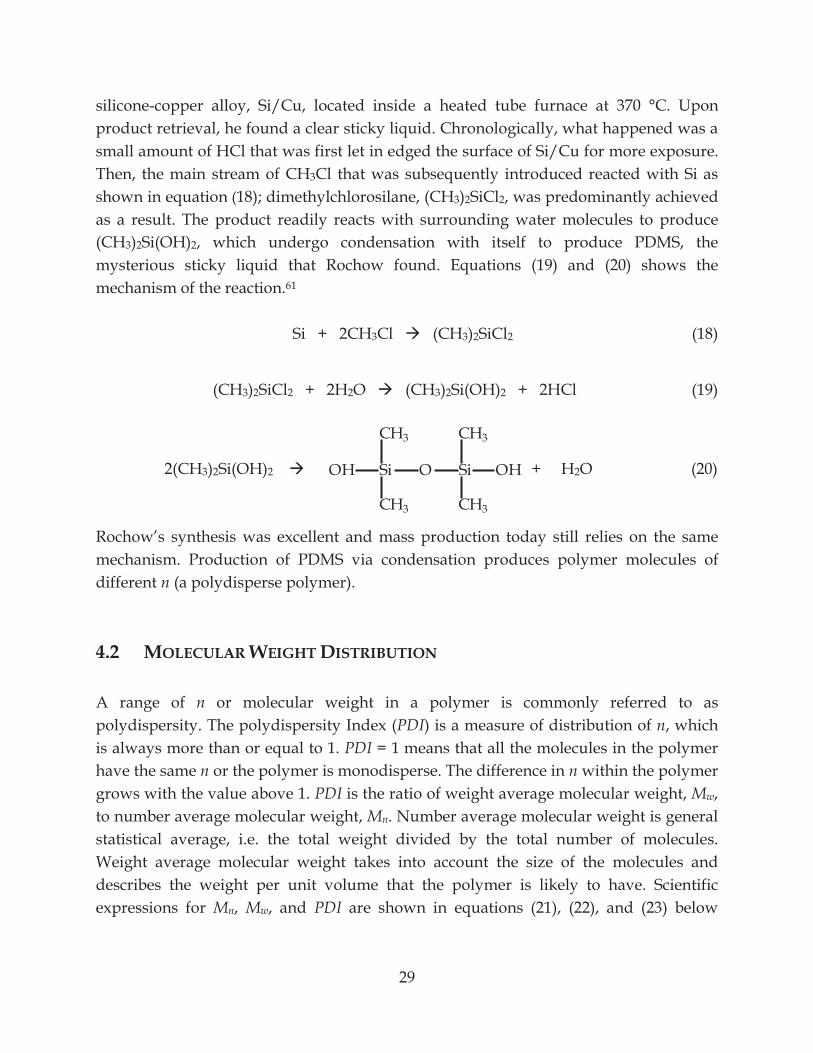
silicone-copper alloy, Si/Cu, located inside a heated tube furnace at 370 °C. Upon product retrieval, he found a clear sticky liquid. Chronologically, what happened was a small amount of HCl that was first let in edged the surface of Si/Cu for more exposure. Then, the main stream of CH3Cl that was subsequently introduced reacted with Si as shown in equation (18); dimethylchlorosilane, (CH3)2SiCl2, was predominantly achieved as a result. The product readily reacts with surrounding water molecules to produce (CH3)2Si(OH)2, which undergo condensation with itself to produce PDMS, the mysterious sticky liquid that Rochow found. Equations (19) and (20) shows the mechanism of the reaction.61

Si + 2CH3Cl (CH3)2SiCl2 (18)

(CH3)2SiCl2 + 2H2O (CH3)2Si(OH)2 + 2HCl (19)

Rochow’s synthesis was excellent and mass production today still relies on the same mechanism. Production of PDMS via condensation produces polymer molecules of different n (a polydisperse polymer). 4.2 MOLECULAR WEIGHT DISTRIBUTION A range of n or molecular weight in a polymer is commonly referred to as polydispersity. The polydispersity Index (PDI) is a measure of distribution of n, which is always more than or equal to 1. PDI = 1 means that all the molecules in the polymer have the same n or the polymer is monodisperse. The difference in n within the polymer grows with the value above 1. PDI is the ratio of weight average molecular weight, Mw, to number average molecular weight, Mn. Number average molecular weight is general statistical average, i.e. the total weight divided by the total number of molecules. Weight average molecular weight takes into account the size of the molecules and describes the weight per unit volume that the polymer is likely to have. Scientific expressions for Mn, Mw, and PDI are shown in equations (21), (22), and (23) below

30

(21)

(22)

(23)

where Ni and wi are the number of and the weight fraction of molecules having the weight Mi:

Mn = NiMiiNii

,

Mw =NiMi

2i

NiMii= wiMi

i

, where wi = NiMi

NiMii ,

PDI = Mw

Mn .

A supply of monodisperse PDMS samples each with a different n would be ideal for experiments in this thesis because they would enable us to make solutions with any n distribution; they are obtainable via anionic polymerization.63 the PDMS sample used in this thesis was polydisperse, although the PDI was small compared to that obtained after mixing with OMTS. The most conventional technique used to determine molecular weights and polydispersity of polymers is size exclusion chromatography (SEC), more specifically Gel Permeation Chromatography (GPC), so named because the stationary phase is a gel. The GPC uses low affinity, nonionic, porous gel columns to separate polymer molecules based on their radius of gyration in the solvent. Small molecules have to traverse through the pores while larger molecules can bypass them, therefore the largest molecules take the least time to dilute. The GPC detects eluents of the column from a property such as concentration, infrared absorbance intensity, refractive index, or molecular dimensions. Results are compared to a result from a standard polymer and converted Mn, Mw, and PDI. 4.3 MECHANICAL BEHAVIOR The viscosity of a polymer melt generally increases with the degree of polymerization, n, because higher n brings about more chain entanglements. Polymers can remain a viscous melt at room temperature up to a certain degree of polymerization, corresponding to a critical molecular weight, Mc. At greater molecular weights, polymers become more solidified and exhibit mechanical properties such as toughness

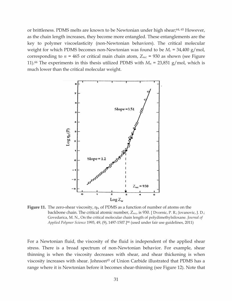
31

or brittleness. PDMS melts are known to be Newtonian under high shear;64, 65 However, as the chain length increases, they become more entangled. These entanglements are the key to polymer viscoelasticity (non-Newtonian behaviors). The critical molecular weight for which PDMS becomes non-Newtonian was found to be Mc = 34,400 g/mol,corresponding to n = 465 or critical main chain atom, Zwc = 930 as shown (see Figure 11).66 The experiments in this thesis utilized PDMS with Mn = 23,851 g/mol, which is much lower than the critical molecular weight.

Figure 11. The zero- 0, of PDMS as a function of number of atoms on the

backbone chain. The critical atomic number, Zwc, is 930. [ Dvornic, P. R.; Jovanovic, J. D.; Govedarica, M. N., On the critical molecular chain length of polydimethylsiloxane. Journal of Applied Polymer Science 1993, 49, (9), 1497-1507.]66 (used under fair use guidelines, 2011)

For a Newtonian fluid, the viscosity of the fluid is independent of the applied shear stress. There is a broad spectrum of non-Newtonian behavior. For example, shear thinning is when the viscosity decreases with shear, and shear thickening is when viscosity increases with shear. Johnson65 of Union Carbide illustrated that PDMS has a range where it is Newtonian before it becomes shear-thinning (see Figure 12). Note that

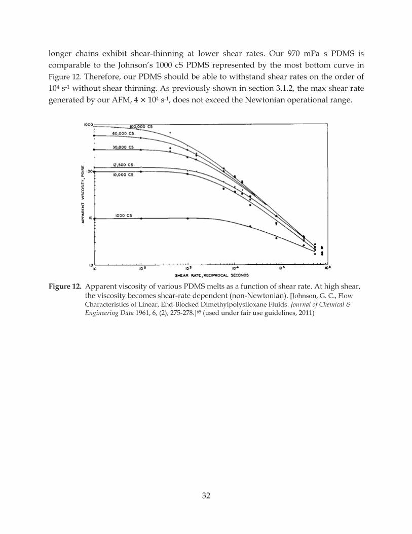
32

longer chains exhibit shear-thinning at lower shear rates. Our 970 mPa s PDMS is comparable to the Johnson’s 1000 cS PDMS represented by the most bottom curve in Figure 12. Therefore, our PDMS should be able to withstand shear rates on the order of 104 s-1 without shear thinning. As previously shown in section 3.1.2, the max shear rate generated by our AFM, 4 × 104 s-1, does not exceed the Newtonian operational range.

Figure 12. Apparent viscosity of various PDMS melts as a function of shear rate. At high shear,

the viscosity becomes shear-rate dependent (non-Newtonian). [Johnson, G. C., Flow Characteristics of Linear, End-Blocked Dimethylpolysiloxane Fluids. Journal of Chemical & Engineering Data 1961, 6, (2), 275-278.]65 (used under fair use guidelines, 2011)

33

(24)

(25)

(26)

Chapter 5 MODELING OF PDMS MELTS AT SOLID-LIQUID

INTERFACES 5.1 CHAIN FRACTIONATION AT INTERFACES AT EQUILIBRIUM When a polymer melt containing chemically identical monomers but differing in n adsorbs at an interface, it is predicted that the equilibrium composition at the interface varies from the bulk: the longer chains are predicted to be more concentrated at the interface than the shorter chains.67, 68 The driving force for this surface effect is the increase in translational entropy in bulk when the long chains adsorb. This effect has been demonstrated by Santore and Fu69 for polystyrene adsorption of a microscope slide, and we would expect the same effect for PDMS on our hydrophobic TMCS-silica. To verify that the PDMS polymer did adsorb preferentially, we examined the surface tension of the PDMS and OMTS on the TMCS-silica: a lower surface tension for PDMS than OMTS would indicate preferential adsorption. The Young’s Laplace equations for PDMS on TMCS-silica in air and for the OMTS on the same substrate in air are as follows:

PDMS-A cos PDMS = S-A- S-PDMS ,

OMTS-A cos OMTS = S-A- S-OMTS , where the surface tensions between PDMS and air, between OMTS and air, between TMCS-silica and air, between TMCS-silica and PDMS, and between TMCS-silica and OMTS are represented by PDMS-A, OMTS-A, S-A, S-PDMS, and S-OMTS, respectively. Contact angles of PDMS and OMTS on TMCS-silica are represented by PDMS and OMTS. Known surface tension values are PDMS-A = 21 dyn/cm and OMTS-A = 15 dyn/cm,70 and contact angles that I measured using the FTA 100 contact angle analyzer are PDMS = 13° and

OMTS = 6°. Assuming that S-A is identical in both PDMS and OMTS, the difference between S-PDMS and S-OMTS is calculated from equation (24) -equation (25):

S-PDMS - S-OMTS= OMTS-A cos OMTS - PDMS A cos PDMS = - 5.5 dyn/cm. The negative value shows that the surface tension between PDMS and glass is lower than that between OMTS and glass. Therefore, we would not expect the OMTS to

34

(27)

(28)

(29)

preferentially adsorb and a greater equilibrium concentration of OMTS at the interface should not be used to explain a reduced lubrication force.

5.2 SHEAR-INDUCED CHAIN FRACTIONATION

If the shear stress varies from point to point in the system (e.g. depends on radial position in capillary flow), then it is possible that the distribution of molecular weights in a mixture will vary from point to point in response to the shear stress. Tirrell and Malone1 found that it is more entropically favorable for longer chains to migrate to the lower shear stress area than to remain in the high-shear flow. For flow through a capillary, the shear stress is greatest near the walls; Tirrell and Malone postulated that the greatest viscosity would be at the center and the lowest at the walls given adequate residence time of polymer in the capillary. A fully developed flow is the key to induce chain fractionation. Tirrell and Malone calculated the conditions for fully-developed flow based on the ratio of length, z, to diameter, D, of the vessel as follows:

zD = - ( ln )Pe

2 02 ,

where Pe is the Peclet number and is a dimensionless number that defines the flow based on the pipe radius, R, flow velocity, vm, and polymer diffusion coefficient, Ð: Pe = vmR/Ð . The fraction of the flow that is yet to be fully developed is symbolized by . Therefore, the developed fraction of flow is defined by 1 – ; for instance, in a 66% developed flow, 0.66 = 1 – and = 0.34. The eigenvalue of the flow, 0

2, is an approximation based on the molecular parameter, , and the smallest eigenvalue, 0*2:1

0*2= 0

2/4 2 . The smallest eigenvalue can be approximated if the molecular parameter, , is known: =

83

vm

R2

2 ,

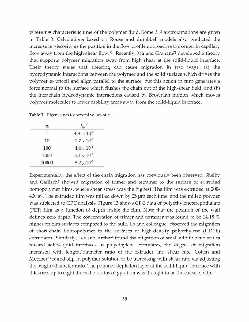
35

where Some 0*2 approximations are given in Table 3. Calculations based on Rouse and dumbbell models also predicted the increase in viscosity as the position in the flow profile approaches the center in capillary flow away from the high-shear flow.71 Recently, Ma and Graham72 developed a theory that supports polymer migration away from high shear at the solid-liquid interface. Their theory states that shearing can cause migration in two ways: (a) the hydrodynamic interactions between the polymer and the solid surface which drives the polymer to uncoil and align parallel to the surface, but this action in turn generates a force normal to the surface which flushes the chain out of the high-shear field, and (b) the intrachain hydrodynamic interactions caused by Brownian motion which moves polymer molecules to lower mobility areas away from the solid-liquid interface. Table 3. Eigenvalues for several values of

Experimentally, the effect of the chain migration has previously been observed. Shelby and Caflisch2 showed migration of trimer and tetramer to the surface of extruded homopolymer films, where shear stress was the highest. The film was extruded at 200-400 s-1. The extruded film was milled down by 25 m each time, and the milled powder was subjected to GPC analysis. Figure 13 shows GPC data of polyethyleneterephthalate (PET) film as a function of depth inside the film. Note that the position of the wall defines zero depth. The concentration of trimer and tetramer was found to be 14-18 % higher on film surfaces compared to the bulk. Lo and colleague3 observed the migration of short-chain fluoropolymer to the surfaces of high-density polyethylene (HDPE) extrudates . Similarly, Lee and Archer4 found the migration of small additive molecules toward solid-liquid interfaces in polyethylene extrudates; the degree of migration increased with length/diameter ratio of the extruder and shear rate. Cohen and Metzner73 found slip in polymer solution to be increasing with shear rate via adjusting the length/diameter ratio. The polymer depletion layer at the solid-liquid interface with thickness up to eight times the radius of gyration was thought to be the cause of slip.

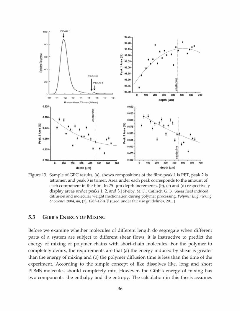
36

Figure 13. Sample of GPC results, (a), shows compositions of the film: peak 1 is PET, peak 2 is

tetramer, and peak 3 is trimer. Area under each peak corresponds to the amount of each component in the film. In 25- m depth increments, (b), (c) and (d) respectively display areas under peaks 1, 2, and 3.[ Shelby, M. D.; Caflisch, G. B., Shear field induced diffusion and molecular weight fractionation during polymer processing. Polymer Engineering & Science 2004, 44, (7), 1283-1294.]2 (used under fair use guidelines, 2011)

5.3 GIBB’S ENERGY OF MIXING Before we examine whether molecules of different length do segregate when different parts of a system are subject to different shear flows, it is instructive to predict the energy of mixing of polymer chains with short-chain molecules. For the polymer to completely demix, the requirements are that (a) the energy induced by shear is greater than the energy of mixing and (b) the polymer diffusion time is less than the time of the experiment. According to the simple concept of like dissolves like, long and short PDMS molecules should completely mix. However, the Gibb’s energy of mixing has two components: the enthalpy and the entropy. The calculation in this thesis assumes

37

(30)

(31)

(32)

that the enthalpy of mixing, mixH, is 0 because the polymer and OMTS (trimer) are the mixS must also be calculated. For this, the Flory-Huggins theory is

used. 5.3.1 Flory-Huggins Theory In 1941, Flory74 and Huggins75 separately discovered the ideal solution theory could not account for solutions containing long chain compounds and paved the way for polymer thermodynamics. After an extensive list of assumptions, they arrived at a conclusion that when molecules of solute and solvent have the same chemistry but are vastly different in n, the Gibb’s fr mixG, is given by a simple algebraic equation:

mixGRT = N1 ln 1

* + N2 ln 2* , where

1* = N1

N1+ rN2; 2

* = rN2

N1+ rN2 .

The numbers of solvent and polymer molecules are represented by N1 and N2, respectively. The polymer is assumed to be made up on average of of r segments, each segment is the size of a single solvent molecule. Thus, the solution contains rN2+N1 lattice sites, and 1

* and 2* represent fractions of sites occupied by solvent and polymer

molecules, equation (31). The absolute temperature of the mixture and gas constant are represented by T and R, respectively. The Flory-Huggins theory assumes that the solution is athermal, i.e. the enthalpy of mixing is zero. This is a reasonable assumption for a homopolymer but does not account for the fact that the chain ends have slightly different chemistry to the rest of the polymer. The polymer component has no crystalinity, i.e. amorphous. The ratio of molar volume of polymer, 1, to that of solvent, 2, is similar to the value of r. 5.3.2 Real Polymer Solutions For real polymer solutions, the Flory-Huggins interaction parameter, , is introduced to account for the enthalpy of mixing. The Gibb’s free energy is then:

mixGRT = N1 ln 1

* + N2 ln 2 * + 1*

2 * (N1+ rN2).

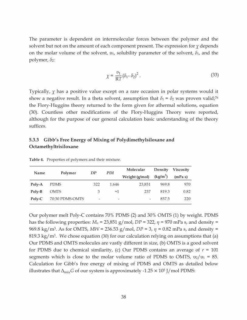
38

(33)

The parameter is dependent on intermolecular forces between the polymer and the solvent but not on the amount of each component present. The expression for depends on the molar volume of the solvent, 1, solubility parameter of the solvent, 1, and the polymer, 2:

= 1

RT ( 1- 2)2 . Typically, has a positive value except on a rare occasion in polar systems would it show a negative result. In a theta solvent, assumption that 1 = 2 was proven valid;76 the Flory-Huggins theory returned to the form given for athermal solutions, equation (30). Countless other modifications of the Flory-Huggins Theory were reported, although for the purpose of our general calculation basic understanding of the theory suffices. 5.3.3 Gibb’s Free Energy of Mixing of Polydimethylsiloxane and Octamethyltrisiloxane Table 4. Properties of polymers and their mixture.

Our polymer melt Poly-C contains 70% PDMS (2) and 30% OMTS (1) by weight. PDMS has the following properties: Mn = 23,851 g/mol, DP = 322, = 970 mPa s, and density = 969.8 kg/m3. As for OMTS, MW = 236.53 g/mol, DP = 3, = 0.82 mPa s, and density = 819.3 kg/m3. We chose equation (30) for our calculation relying on assumptions that (a) Our PDMS and OMTS molecules are vastly different in size, (b) OMTS is a good solvent for PDMS due to chemical similarity, (c) Our PDMS contains an average of r = 101 segments which is close to the molar 2 1 = 85. Calculation for Gibb’s free energy of mixing of PDMS and OMTS as detailed below illustrates that mixG of our system is approximately -1.25 × 105 J/mol PDMS:

Molecular Density Viscosity

Weight (g/mol) (kg/m3) (mPa s)

Poly-A PDMS 322 1.646 23,851 969.8 970

Poly-B OMTS 3 237 819.3 0.82

Poly-C 70:30 PDMS-OMTS - - - 857.5 220

Name Polymer DP PDI

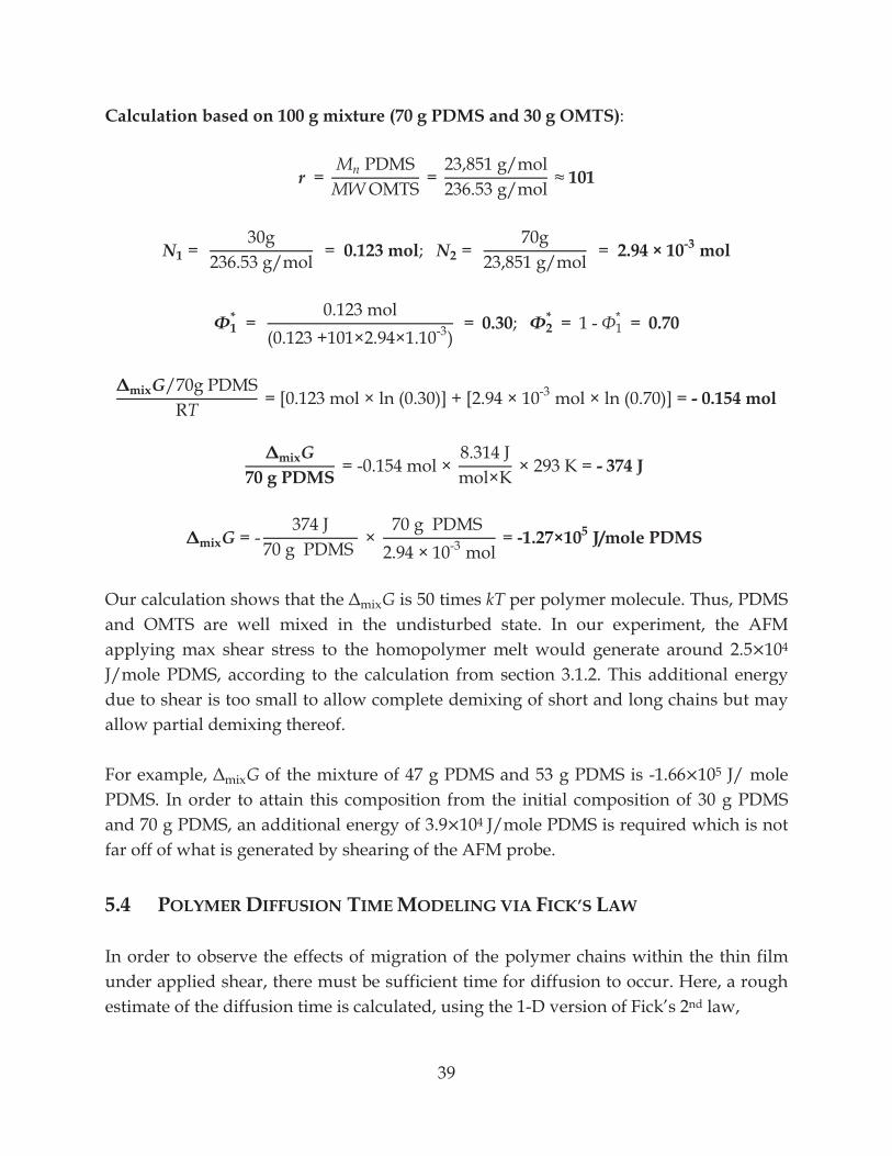
39

Calculation based on 100 g mixture (70 g PDMS and 30 g OMTS):

r = Mn PDMS

MW OMTS = 23,851 g/mol236.53 g/mol 101

N1 = 30g

236.53 g/mol = 0.123 mol; N2 = 70g

23,851 g/mol = 2.94 × 10-3 mol

1* = 0.123 mol

(0.123 +101×2.94×1.10-3) = 0.30; 2

* = 1 - 1* = 0.70

mixG/70g PDMS

RT = [0.123 mol × ln (0.30)] + [2.94 × 10-3 mol × ln (0.70)] = - 0.154 mol

mixG

70 g PDMS = -0.154 mol × 8.314 Jmol×K × 293 K = - 374 J

mixG = -374 J

70 g PDMS × 70 g PDMS

2.94 × 10-3 mol = --1.27×105 J/mole PDMS

Our calculation shows that the mixG is 50 times kT per polymer molecule. Thus, PDMS and OMTS are well mixed in the undisturbed state. In our experiment, the AFM applying max shear stress to the homopolymer melt would generate around 2.5×104 J/mole PDMS, according to the calculation from section 3.1.2. This additional energy due to shear is too small to allow complete demixing of short and long chains but may allow partial demixing thereof. For example, mixG of the mixture of 47 g PDMS and 53 g PDMS is -1.66×105 J/ mole PDMS. In order to attain this composition from the initial composition of 30 g PDMS and 70 g PDMS, an additional energy of 3.9×104 J/mole PDMS is required which is not far off of what is generated by shearing of the AFM probe. 5.4 POLYMER DIFFUSION TIME MODELING VIA FICK’S LAW In order to observe the effects of migration of the polymer chains within the thin film under applied shear, there must be sufficient time for diffusion to occur. Here, a rough estimate of the diffusion time is calculated, using the 1-D version of Fick’s 2nd law,

40

(36)

(35)

(34) ct = Ð

2cx2 ; BC 1: c(0) = c0, BC 2 : c( )= 0 ,

which suggests that PDMS molecules will have enough time during the approach of the sphere toward the plate to diffuse out of the high shear regions. The maximum strain rate occurs at the radial distance x = (2RH/3)1/2,77 where R is the radius of the sphere and H is the sphere-plate separation, so we use x as the required diffusion distance, i.e. the molecules must be able to diffuse on the length scale of x to significantly diminish lubrication force. Note that x is a function of H, thus the diffusion time is also a function of H. The solution is: to diffusion time, t, is given by:

c(x, t) = c(z) = c0(1 – Erf (z)); z = x

2Ðt .

Once all the PDMS molecules diffuse the distance x, its concentration is zero or c(x, t) = 0. The time they take to complete the diffusion is: c(x, t) = 0; t = x2

18Ð . The diffusion coefficient of PDMS is approximated from values reported by Appel and Fleischer78; At 60 °C, Ð60°C = 3.6×10-12 m2/s. For my experiment conducted at 20 °C, Arrhenius extrapolation of diffusion coefficient gives Ð20°C = 3.8×10-13 m2/s. From the diffusion time, we can calculate the maximum drive speed for the sphere approaching the plate to allow for diffusion of PDMS molecules out of the high shear region, i.e. diffuse the distance x . The results are shown in Figure 14. For example, the maximum drive speed used in this thesis v = 120 m/s provides enough time for diffusion out of the high shear region when the film thickness, H, is less than 50 nm. Owing to the deflection of the cantilever, the sphere speed is lower in thin films. Combined with smaller diffusion distances, this ensures adequate diffusion time. Nonetheless, this diffusion model breaks down when thickness of the thin film is close to the size of the PDMS molecules or twice the radius of gyration (Rg = 3.6×10-9 m). PDMS molecules are not likely to reside in this thin-film region (H = 2Rg) where they have to conform to an entropically unfavorable linear formation, Thus, they escape the thin film due to size exclusion rather than diffusion.

41

Figure 14. The graph displays on the primary vertical axis the theoretical estimate of the time it

would take PDMS used in experiments of PDMS-OMTS mixture under shear to diffuse the characteristic distance, x, at selected separations, H. The secondary vertical axis displays the maximum drive speed at selected separation. Driving beyond the maximum speed would not provide enough time for the PDMS to diffuse.

42

Chapter 6 EXPERIMENTAL 6.1 POLYMERS AND HOMOPOLYMER MIXTURE 6.1.1 Properties of Polymers Properties of all polymers used in the following experiments are summarized in Table 4. Polydimethylsiloxane (PDMS), 98% purity octamethyltrisiloxane (OMTS), and 99% purity trimethylchlorosilane (TMCS) obtained from Sigma Aldrich were not purified before testing. Octamethylsiloxane is a trimer of PDMS so will henceforth be referred to as “trimer”. PDMS had the weight and number average molecular weights Mw = 39,260 g/mol, Mn = 23,851 g/mol and viscosity = 970 mPa s. The poly dispersity result from GPC showed a single molecular weight peak with PDI = 1.646. Viscosity of the trimer was 0.82 mPa s. Our homopolymer mixture, Poly-C, consisted of 70 weight% PDMS and 30 weight% trimer by weight ( = 220 mPa s) and was made in-house.

6.1.2 Viscosity Measurements of Mixtures of Various Compositions Five homopolymer mixture compositions were made. Presenting in terms of weight% of PDMS to trimer, the compositions were 50:50, 60:40, 70:30 (Poly-C), 80:20, and 90:10. The viscosities of these mixtures are used to compare with viscosities of Poly-C under shear to decipher whether there is a change in the composition and what that changed composition might be. An Ubbelohde capillary viscometer was calibrated with the PDMS melt to obtain a constant, . Viscosities of the mixtures are the product of and the time it takes for each mixture to flow through the capillary.

6.2 PREPARATION OF GLASS SUBSTRATES 6.2.1 Surface Preparation Glass plates from Fisher Scientific were utilized as the flat planar substrate. Prior to the experiments, the plates were rinsed with water and ethanol and blown dry with nitrogen, and then treated with oxygen plasma for 1 minute at 100 W and 0.3 mbar. Immediately after being removed from the plasma chamber, substrates were transferred into a desiccator and sealed at low pressure. Some plates (TMCS plates) were made hydrophobic by reaction with TMCS. To do so, TMCS (0.5 – 1 mL) was released into the sealed desiccator for 2 hours. Upon removal from the desiccator, substrates were sonicated in toluene for 15 minutes then rinsed with water and ethanol and blown dry with nitrogen to conclude the preparation process.

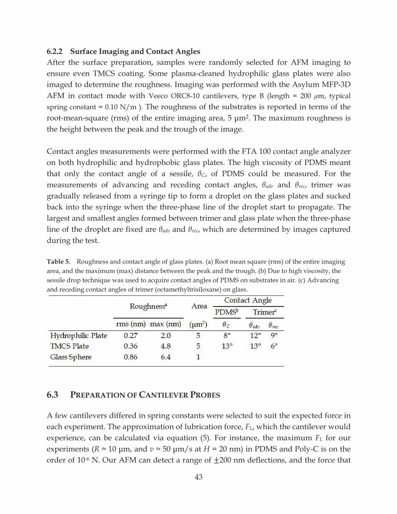
43

6.2.2 Surface Imaging and Contact Angles After the surface preparation, samples were randomly selected for AFM imaging to ensure even TMCS coating. Some plasma-cleaned hydrophilic glass plates were also imaged to determine the roughness. Imaging was performed with the Asylum MFP-3D AFM in contact mode with Veeco ORC8-10 cantilevers, type B (length = 200 m, typical spring constant = 0.10 N/m ). The roughness of the substrates is reported in terms of the root-mean- 2. The maximum roughness is the height between the peak and the trough of the image. Contact angles measurements were performed with the FTA 100 contact angle analyzer on both hydrophilic and hydrophobic glass plates. The high viscosity of PDMS meant that only the contact angle of a sessile, C, of PDMS could be measured. For the measurements of advancing and receding contact angles, adv and rec, trimer was gradually released from a syringe tip to form a droplet on the glass plates and sucked back into the syringe when the three-phase line of the droplet start to propagate. The largest and smallest angles formed between trimer and glass plate when the three-phase line of the droplet are fixed are adv and rec, which are determined by images captured during the test. Table 5. Roughness and contact angle of glass plates. (a) Root mean square (rms) of the entire imaging area, and the maximum (max) distance between the peak and the trough. (b) Due to high viscosity, the sessile drop technique was used to acquire contact angles of PDMS on substrates in air. (c) Advancing and receding contact angles of trimer (octamethyltrisiloxane) on glass.

6.3 PREPARATION OF CANTILEVER PROBES A few cantilevers differed in spring constants were selected to suit the expected force in each experiment. The approximation of lubrication force, FL, which the cantilever would experience, can be calculated via equation (5). For instance, the maximum FL for our experiments (R v H = 20 nm) in PDMS and Poly-C is on the order of 10-6 N. Our AFM can detect a range of ±200 nm deflections, and the force that

44

the cantilever experiences is the spring constant, k, times the deflection. The cantilever needs to have k that deflects ±200 nm in response to the force on the order of 10-6 N, and that minimum k is 2.5 N/m. Thus, we choose cantilevers with k to conduct experiments in PDMS and Poly-C. The two types of rectangular cantilevers selected for experiments in (1) PDMS and Poly-C and (2) trimer are: (1) NT-MDT NSG11/Tipless cantilever, type B (length = 130 m, typical spring constant = 5.5 N/m) and (2) Veeco ORC8-10 cantilever, type D (length = 200 m, typical spring constant = 0.05 N/m ). A borosilicate sphere with nominal radius = 10 m from Duke Scientific was glued to the free end of the cantilever using epoxy glue following the method described in Ducker et al.53 The roughness of the 1- 2 contact area of the spheres was measured via AFM imaging; those with asperities more than ± 5 nm were discarded. Cantilevers were cleaned by dipping in ethanol and water and exposed to a UV source for 1 hour. The preparation process stopped at this point for the “hydrophilic” spheres. For TMCS spheres, the TMCS coating process was the same as for TMCS plates. Afterwards, cantilevers were cleaned in toluene, water and ethanol, respectively. The cantilevers were then imaged again to ensure smooth coating (spheres with roughness > ±5 nm discarded). Attachment of the sphere slightly changes the spring constant of the cantilever. For accurate force calculation, spring constant was calibrated following the method reported in Sader et al79 prior to each AFM force measurement.

6.4 AFM FORCE MEASUREMENTS

The technique for measuring colloidal forces53 and lubrication measurements8 have been previously reported. Force measurements were performed on the Asylum MFP-3D AFM in an open fluid cell. The forces were measured from the deflection of a cantilever spring and the separation was altered by a piezoelectric crystal. The expansion of the crystal was monitored using a linear variable differential transducer (LVDT), and increased approximately linearly with time after initial acceleration. The raw data were deflection (uncalibrated) and LVDT displacement (in nanometers) as a function of time. Two set of raw data were collected in pairs: a fast drive, for analysis of the lubrication force; and a slow drive, for determination of the surface force and calibration. The slow drive was selected on the basis that the lubrication force was negligible. It would be useful at this point to explain all the forces.

45

(37)

(38)

(39)

6.4.1 Forces As a sphere moves through fluid toward a plate and surfaces are in very close proximity, lubrication force, FL, may not be the only force the sphere experiences. The total measured force, Ftotal, is the combination of forces exerted on the sphere, Fsphere, and those exerted on the cantilever, Fdrag:

Ftotal = Fsphere + Fdrag.

Forces exerted on the sphere are lubrication forces, FL, equilibrium forces, Fequil, and inertial force, Finertial:

Fsphere = FL + Fequil + Finertial. Unlike lubrication force, equilibrium surface forces are independent of speed, namely electro-static forces, van der Waals forces, and polymer depletion forces. Therefore, these forces can be observed by driving a sphere slowly toward a plane because the lubrication force component is diminished at this speed. These forces can be taken directly and subtracted off the total force from the high-speed run to obtain the lubrication force, although no equilibrium forces were found in the slow runs of our experiments. Our experiments are also unaffected by the inertial force because the acceleration of the sphere is too slow for inertia to be felt. Nonetheless, the cantilever drag force, Fdrag, is known to be speed dependent. Moreover, we found it to be increasingly dependent on the sphere-plane separation, H, as the two surfaces get closer. It is necessary to conduct a separate experiment to determine the cantilever damping coefficient, A, which is viscosity- and cantilever-specific. In such experiment, forces, Fin and Fout, are measured while a cantilever without a sphere attached is driven through fluid toward and away from a plane at velocities vin and vout, respectively. The cantilever drag force is the product of the damping coefficient at separation equal to twice the radius of the sphere plus the sphere-plane separation (where the cantilever is located in the actual experiment), A|H’ = 2R+H, and the velocity of the sphere in the actual experiment, vsphere:

Fdrag(H') = A|H' = 2R+H vsphere= Fin - Fout

vin- vout H' = 2R+H vsphere

46

Once the cantilever drag force is subtracted off the total force, the remaining lubrication force can be related back to equation (5) or (6) for slip quantification. The cantilever damping coefficient reduces with separation. Thus, the use of larger sphere can reduce the cantilever drag force. However, we have yet to find a company that produces spheres of R ±5 nm maximum roughness.

6.4.2 Measurement of Forces 1) The deflection of the cantilever was calibrated from the slope of the deflection voltage vs LVDT plot in a slow run, which produces the constant commonly described as invols. (Calibration of the deflection in a fast run is difficult because the lubrication force asymptotes to large values at small separations, so it is difficult to determine where the probe contacts the plate). In previous work, we used the average invols of the approach and retract curves,8, 56 but in this work, the two values were indistinguishable.

2) The LVDT range of zero of separation in the fast run was determined from a plot of separation vs time. The zero separation was where the separation remained constant with time even through the piezo was driving toward the surface. For this to occur, the deflection must equal the LVDT signal. The separation for this stage was calculated as the sum of the LVDT signal and the deflection that was calibrated as described in 1), using the slow run.

3) A correction was made for virtual deflection. A section of a fast run was examined at large separation, where the lubrication was negligible. The average of the approach and retract curves was determined as a function of LVDT, and fitted to a line. This line was then subtracted from the entire deflection-LVDT signal. This was typically a small correction in the region were the lubrication force was substantial. Correction for virtual deflection on a slow run, following the procedure for the fast run, was found only changed the invols by 0.3%; it was therefore unnecessary.

4) The total force, Ftotal (see equation (37)), on the cantilever is the sum of (i) the lubrication force, FL, on the sphere, (ii) the static force, Fequil, on the sphere (negligible), (iii) the inertial force, Finertial, on the sphere (negligible), and (iv) the force on the cantilever, Fdrag. To obtain the lubrication force on the sphere, (ii), (iii) and (iv) must be subtracted from the total force. The estimation of the force on the cantilever was different to that made by Honig and Ducker.8 Pairs of measurements under matching conditions were made (A) on cantilever with spheres and (B) on cantilevers of the same type, but without a sphere. Results from (B) were used to estimate the contribution of

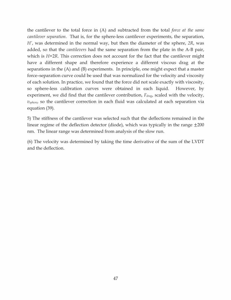
47

the cantilever to the total force in (A) and subtracted from the total force at the same cantilever separation. That is, for the sphere-less cantilever experiments, the separation, H’, was determined in the normal way, but then the diameter of the sphere, 2R, was added, so that the cantilevers had the same separation from the plate in the A-B pair, which is H+2R. This correction does not account for the fact that the cantilever might have a different shape and therefore experience a different viscous drag at the separations in the (A) and (B) experiments. In principle, one might expect that a master force–separation curve could be used that was normalized for the velocity and viscosity of each solution. In practice, we found that the force did not scale exactly with viscosity, so sphere-less calibration curves were obtained in each liquid. However, by experiment, we did find that the cantilever contribution, Fdrag, scaled with the velocity, vsphere, so the cantilever correction in each fluid was calculated at each separation via equation (39).

5) The stiffness of the cantilever was selected such that the deflections remained in the linear regime of the deflection detector (diode), which was typically in the range ±200 nm. The linear range was determined from analysis of the slow run.

(6) The velocity was determined by taking the time derivative of the sum of the LVDT and the deflection.

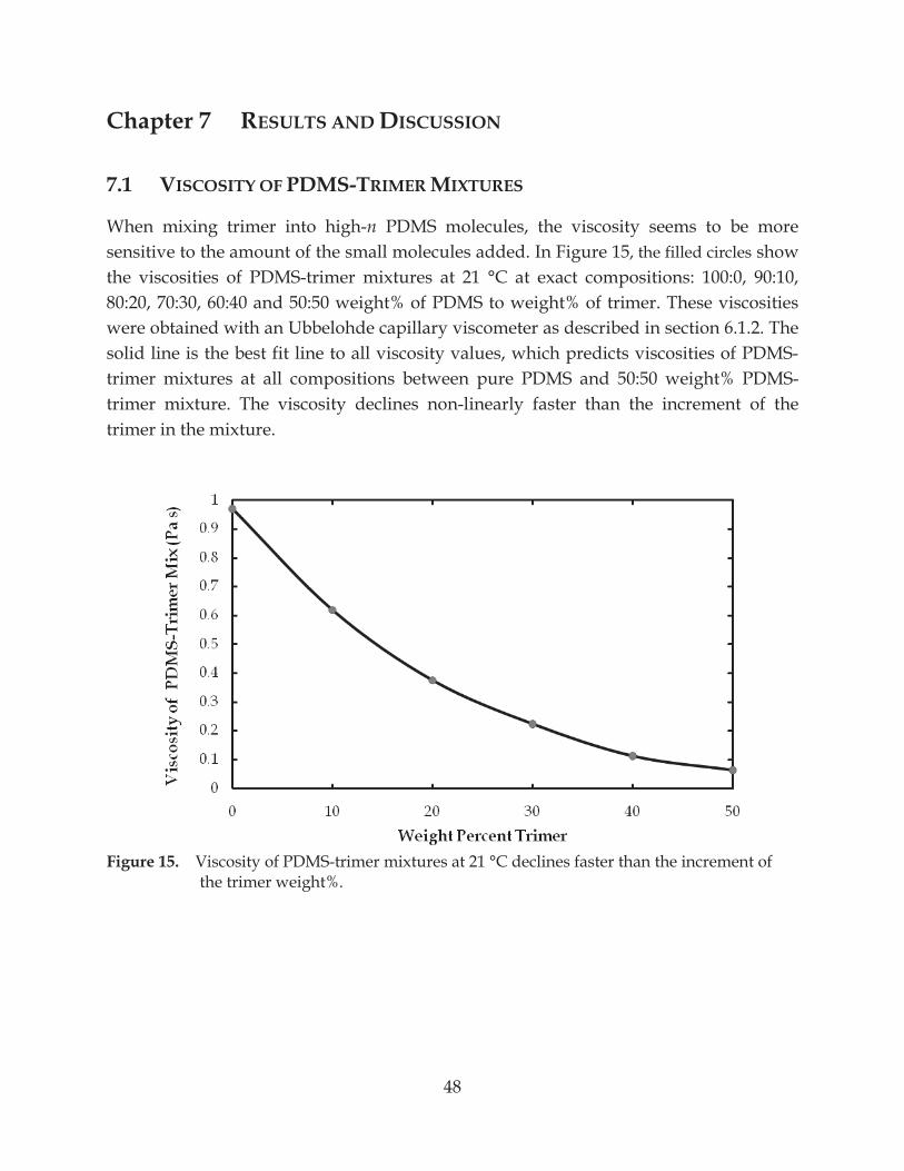
48

Chapter 7 RESULTS AND DISCUSSION

7.1 VISCOSITY OF PDMS-TRIMER MIXTURES

When mixing trimer into high-n PDMS molecules, the viscosity seems to be more sensitive to the amount of the small molecules added. In Figure 15, the filled circles showthe viscosities of PDMS-trimer mixtures at 21 °C at exact compositions: 100:0, 90:10, 80:20, 70:30, 60:40 and 50:50 weight% of PDMS to weight% of trimer. These viscosities were obtained with an Ubbelohde capillary viscometer as described in section 6.1.2. The solid line is the best fit line to all viscosity values, which predicts viscosities of PDMS-trimer mixtures at all compositions between pure PDMS and 50:50 weight% PDMS-trimer mixture. The viscosity declines non-linearly faster than the increment of the trimer in the mixture.

Figure 15. Viscosity of PDMS-trimer mixtures at 21 °C declines faster than the increment of

the trimer weight%.

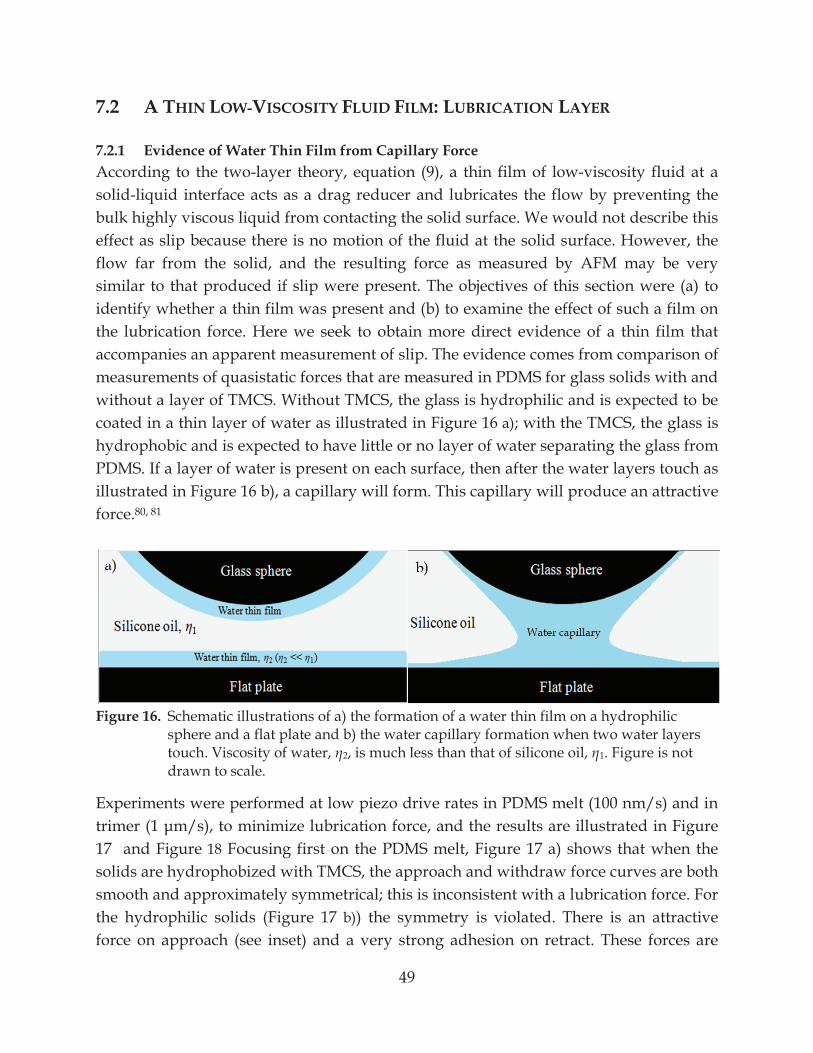
49

7.2 A THIN LOW-VISCOSITY FLUID FILM: LUBRICATION LAYER 7.2.1 Evidence of Water Thin Film from Capillary Force According to the two-layer theory, equation (9), a thin film of low-viscosity fluid at a solid-liquid interface acts as a drag reducer and lubricates the flow by preventing the bulk highly viscous liquid from contacting the solid surface. We would not describe this effect as slip because there is no motion of the fluid at the solid surface. However, the flow far from the solid, and the resulting force as measured by AFM may be very similar to that produced if slip were present. The objectives of this section were (a) to identify whether a thin film was present and (b) to examine the effect of such a film on the lubrication force. Here we seek to obtain more direct evidence of a thin film that accompanies an apparent measurement of slip. The evidence comes from comparison of measurements of quasistatic forces that are measured in PDMS for glass solids with and without a layer of TMCS. Without TMCS, the glass is hydrophilic and is expected to be coated in a thin layer of water as illustrated in Figure 16 a); with the TMCS, the glass is hydrophobic and is expected to have little or no layer of water separating the glass from PDMS. If a layer of water is present on each surface, then after the water layers touch as illustrated in Figure 16 b), a capillary will form. This capillary will produce an attractive force.80, 81

Figure 16. Schematic illustrations of a) the formation of a water thin film on a hydrophilic

sphere and a flat plate and b) the water capillary formation when two water layers touch. Viscosity of water, 2, is much less than that of silicone oil, 1. Figure is not drawn to scale.

Experiments were performed at low piezo drive rates in PDMS melt (100 nm/s) and in /s), to minimize lubrication force, and the results are illustrated in Figure

17 and Figure 18 Focusing first on the PDMS melt, Figure 17 a) shows that when the solids are hydrophobized with TMCS, the approach and withdraw force curves are both smooth and approximately symmetrical; this is inconsistent with a lubrication force. For the hydrophilic solids (Figure 17 b)) the symmetry is violated. There is an attractive force on approach (see inset) and a very strong adhesion on retract. These forces are

50

characteristic of the presence of a capillary.80, 81 The capillary forms on approach (~4 nm), and on the retract it is stretched until it breaks (~60 nm), at which point the cantilever rapidly springs back to its undeflected position. The capillary formation at 4 nm also indicates that the water layer on each surface has a thickness of ~2 nm. Thus, the TMCS treatment can be used to prevent the formation of the capillary.

Figure 17. Force between a glass sphere and a glass plate in PDMS melt. (a) TMCS-glass: piezo drive rate = 100 nm/s, spring constant = 12 N/m , R = 12.5 m. (b) Hydrophilic glass: piezo drive rate = 100 nm/s, spring constant = 6.9 N/m, R = 14.1 m. Note the strong attraction for hydrophilic glass requires a much larger scale for part (b). The inset in b) shows that the capillary formed at ~4 nm, which indicates that the water layer thickness is ~2 nm on each surface.

A similar effect is observed in the liquid trimer. The TMCS glass (Figure 18 a))experiences forces that are approximately symmetrical about the zero force, which is characteristic of a lubrication force, whereas the hydrophilic glass (Figure 18 b))experiences an attraction on approach of the sphere, and a discontinuity on retract. The capillary force on the approach is strong (Note the scale difference in a) and b)), which makes it difficult to point out the separation at which it started or the thickness of the water films.

a) b)

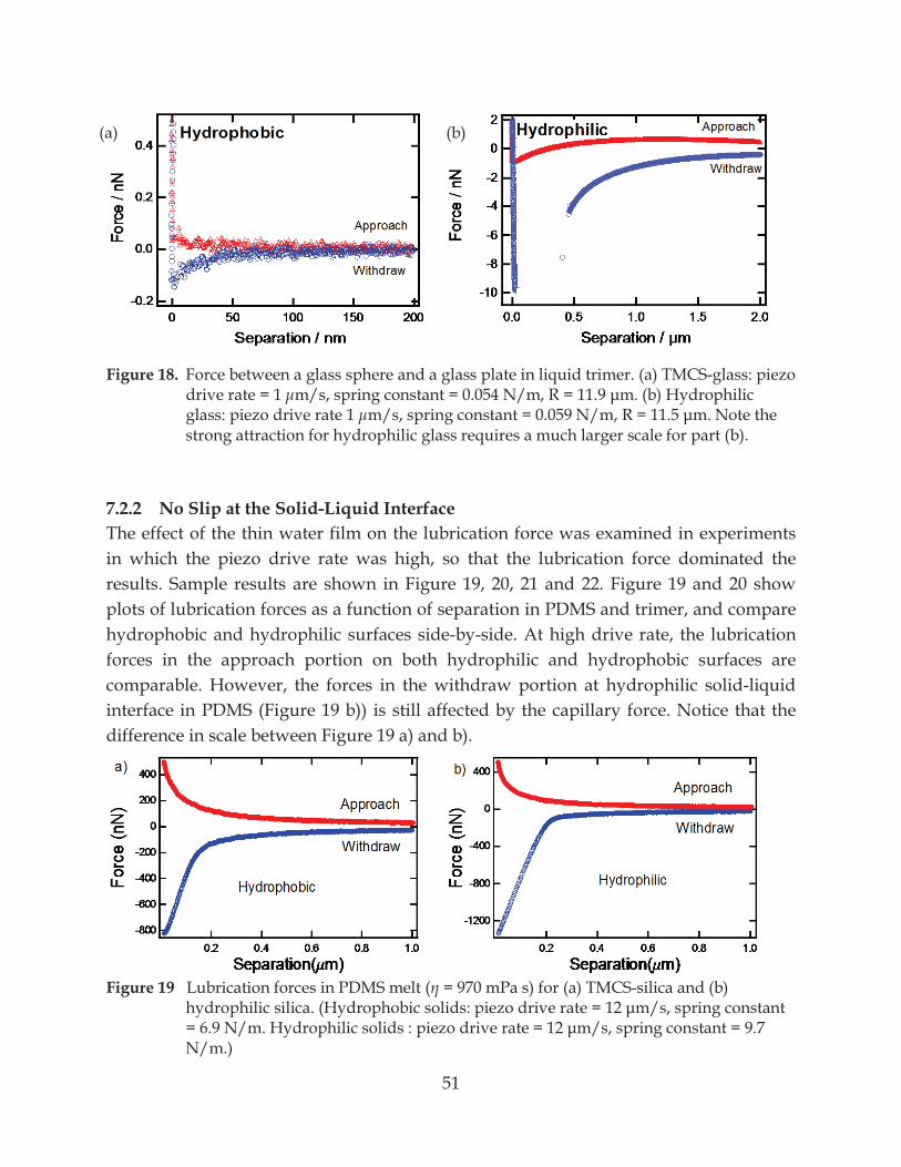
51

Figure 18. Force between a glass sphere and a glass plate in liquid trimer. (a) TMCS-glass: piezo drive rate = 1 m/s, spring constant = 0.054 N/m, R = 11.9 (b) Hydrophilic glass: piezo drive rate 1 strong attraction for hydrophilic glass requires a much larger scale for part (b).

7.2.2 No Slip at the Solid-Liquid Interface The effect of the thin water film on the lubrication force was examined in experiments in which the piezo drive rate was high, so that the lubrication force dominated the results. Sample results are shown in Figure 19, 20, 21 and 22. Figure 19 and 20 show plots of lubrication forces as a function of separation in PDMS and trimer, and compare hydrophobic and hydrophilic surfaces side-by-side. At high drive rate, the lubrication forces in the approach portion on both hydrophilic and hydrophobic surfaces are comparable. However, the forces in the withdraw portion at hydrophilic solid-liquid interface in PDMS (Figure 19 b)) is still affected by the capillary force. Notice that the difference in scale between Figure 19 a) and b).

Figure 19 Lubrication forces in PDMS melt ( = 970 mPa s) for (a) TMCS-silica and (b)

hydrophilic silica. = 6.9 N/m. Hydrophilic solids : piezo N/m.)

(a) (b)

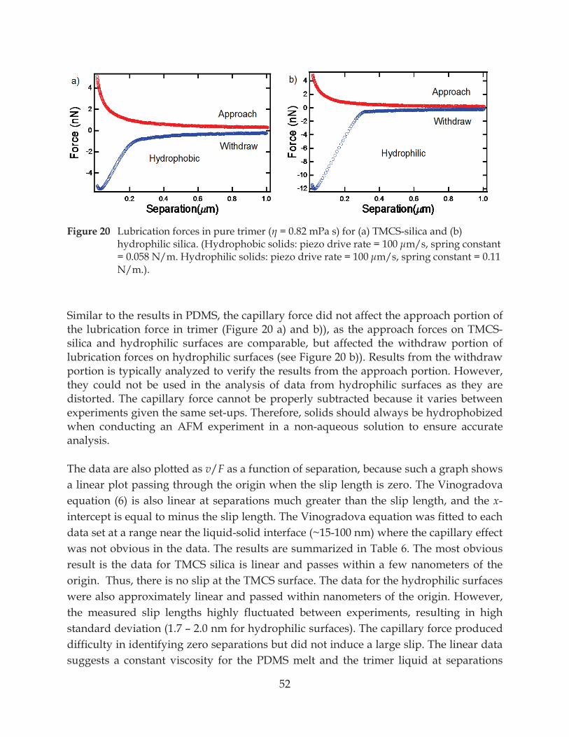
52

Figure 20 Lubrication forces in pure trimer ( = 0.82 mPa s) for (a) TMCS-silica and (b) hydrophilic silica. (Hydrophobic solids: piezo drive rate = 100 m/s, spring constant = 0.058 N/m. Hydrophilic solids: piezo drive rate = 100 m/s, spring constant = 0.11 N/m.).

Similar to the results in PDMS, the capillary force did not affect the approach portion of the lubrication force in trimer (Figure 20 a) and b)), as the approach forces on TMCS-silica and hydrophilic surfaces are comparable, but affected the withdraw portion of lubrication forces on hydrophilic surfaces (see Figure 20 b)). Results from the withdraw portion is typically analyzed to verify the results from the approach portion. However, they could not be used in the analysis of data from hydrophilic surfaces as they are distorted. The capillary force cannot be properly subtracted because it varies between experiments given the same set-ups. Therefore, solids should always be hydrophobized when conducting an AFM experiment in a non-aqueous solution to ensure accurate analysis.

The data are also plotted as v/F as a function of separation, because such a graph shows a linear plot passing through the origin when the slip length is zero. The Vinogradova equation (6) is also linear at separations much greater than the slip length, and the x-intercept is equal to minus the slip length. The Vinogradova equation was fitted to each data set at a range near the liquid-solid interface (~15-100 nm) where the capillary effect was not obvious in the data. The results are summarized in Table 6. The most obvious result is the data for TMCS silica is linear and passes within a few nanometers of the origin. Thus, there is no slip at the TMCS surface. The data for the hydrophilic surfaces were also approximately linear and passed within nanometers of the origin. However, the measured slip lengths highly fluctuated between experiments, resulting in high standard deviation (1.7 – 2.0 nm for hydrophilic surfaces). The capillary force produced difficulty in identifying zero separations but did not induce a large slip. The linear data suggests a constant viscosity for the PDMS melt and the trimer liquid at separations

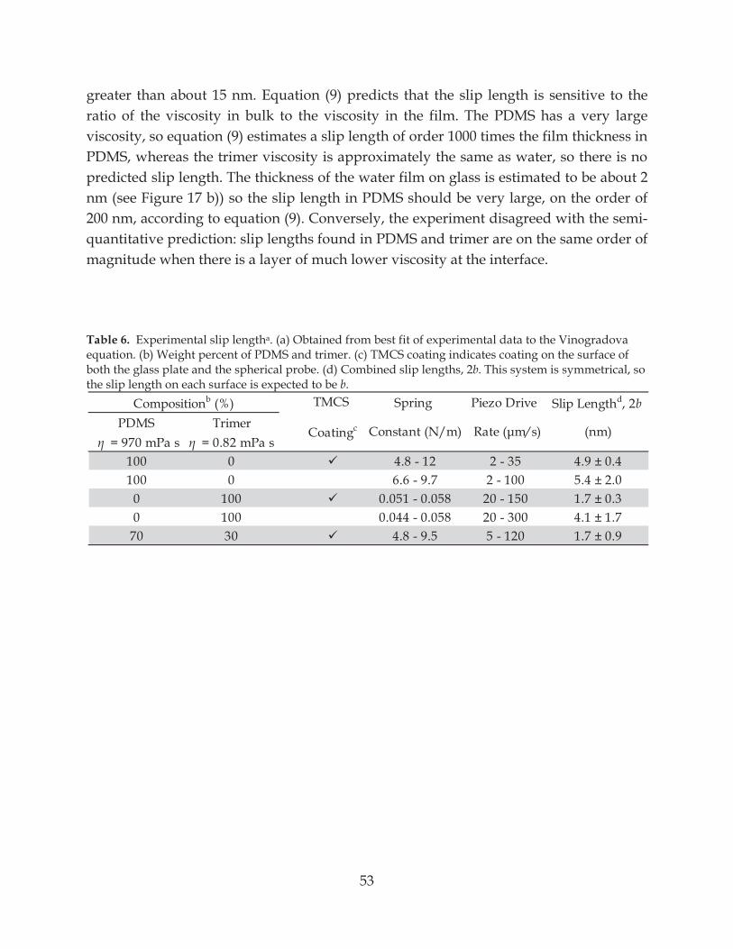
53

greater than about 15 nm. Equation (9) predicts that the slip length is sensitive to the ratio of the viscosity in bulk to the viscosity in the film. The PDMS has a very large viscosity, so equation (9) estimates a slip length of order 1000 times the film thickness in PDMS, whereas the trimer viscosity is approximately the same as water, so there is no predicted slip length. The thickness of the water film on glass is estimated to be about 2 nm (see Figure 17 b)) so the slip length in PDMS should be very large, on the order of 200 nm, according to equation (9). Conversely, the experiment disagreed with the semi-quantitative prediction: slip lengths found in PDMS and trimer are on the same order of magnitude when there is a layer of much lower viscosity at the interface. Table 6. Experimental slip lengtha. (a) Obtained from best fit of experimental data to the Vinogradova equation. (b) Weight percent of PDMS and trimer. (c) TMCS coating indicates coating on the surface of both the glass plate and the spherical probe. (d) Combined slip lengths, 2b. This system is symmetrical, so the slip length on each surface is expected to be b.

Spring Piezo Drive Slip Lengthd, 2bPDMS Trimer

= 970 mPa s = 0.82 mPa s100 0 4.8 - 12 2 - 35 4.9 ± 0.4100 0 6.6 - 9.7 2 - 100 5.4 ± 2.0

0 100 0.051 - 0.058 20 - 150 1.7 ± 0.30 100 0.044 - 0.058 20 - 300 4.1 ± 1.7

70 30 4.8 - 9.5 5 - 120 1.7 ± 0.9

(nm)

Compositionb (%) TMCS

Coatingc Constant (N/m) / s)

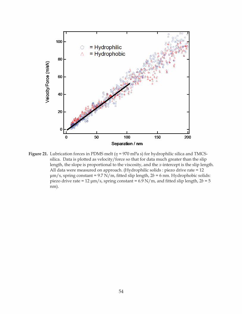
54

Figure 21. Lubrication forces in PDMS melt ( = 970 mPa s) for hydrophilic silica and TMCS-silica. Data is plotted as velocity/force so that for data much greater than the slip length, the slope is proportional to the viscosity, and the x-intercept is the slip length. All data were measured on approach. (Hydrophilic solids : piezo drive rate = 12

b = 6 nm. Hydrophobic solids: b = 5

nm).

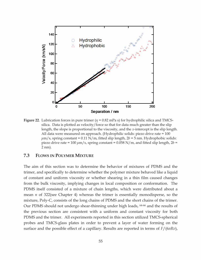
55

Figure 22. Lubrication forces in pure trimer ( = 0.82 mPa s) for hydrophilic silica and TMCS-silica. Data is plotted as velocity/force so that for data much greater than the slip length, the slope is proportional to the viscosity, and the x-intercept is the slip length. All data were measured on approach. (Hydrophilic solids: piezo drive rate = 100

m/s, spring constant = 0.11 N/m, fitted slip length, 2b = 5 nm. Hydrophobic solids: piezo drive rate = 100 m/s, spring constant = 0.058 N/m, and fitted slip length, 2b = 2 nm).

7.3 FLOWS IN POLYMER MIXTURE The aim of this section was to determine the behavior of mixtures of PDMS and the trimer, and specifically to determine whether the polymer mixture behaved like a liquid of constant and uniform viscosity or whether shearing in a thin film caused changes from the bulk viscosity, implying changes in local composition or conformation. The PDMS itself consisted of a mixture of chain lengths, which were distributed about a mean n of 322(see Chapter 4) whereas the trimer is essentially monodisperse, so the mixture, Poly-C, consists of the long chains of PDMS and the short chains of the trimer. Our PDMS should not undergo shear-thinning under high loads, 64-66 and the results of the previous section are consistent with a uniform and constant viscosity for both PDMS and the trimer. All experiments reported in this section utilized TMCS-spherical probes and TMCS-glass plates in order to prevent a layer of water forming on the surface and the possible effect of a capillary. Results are reported in terms of F/(6 Rv),

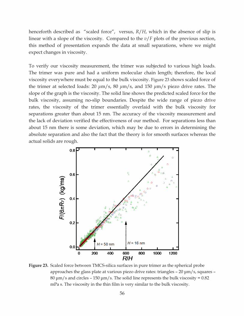
56

henceforth described as “scaled force”, versus, R/H, which in the absence of slip is linear with a slope of the viscosity. Compared to the v/F plots of the previous section, this method of presentation expands the data at small separations, where we might expect changes in viscosity. To verify our viscosity measurement, the trimer was subjected to various high loads. The trimer was pure and had a uniform molecular chain length; therefore, the local viscosity everywhere must be equal to the bulk viscosity. Figure 23 shows scaled force of the trimer at selected loads: 20 m/s, 80 m/s, and 150 m/s piezo drive rates. The slope of the graph is the viscosity. The solid line shows the predicted scaled force for the bulk viscosity, assuming no-slip boundaries. Despite the wide range of piezo drive rates, the viscosity of the trimer essentially overlaid with the bulk viscosity for separations greater than about 15 nm. The accuracy of the viscosity measurement and the lack of deviation verified the effectiveness of our method. For separations less than about 15 nm there is some deviation, which may be due to errors in determining the absolute separation and also the fact that the theory is for smooth surfaces whereas the actual solids are rough.

Figure 23. Scaled force between TMCS-silica surfaces in pure trimer as the spherical probe

approaches the glass plate at various piezo drive rates: triangles – – cles –

mPa s. The viscosity in the thin film is very similar to the bulk viscosity.

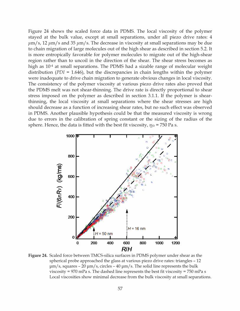
57

Figure 24 shows the scaled force data in PDMS. The local viscosity of the polymer stayed at the bulk value, except at small separations, under all piezo drive rates: 4

m/s, 12 m/s and 35 m/s. The decrease in viscosity at small separations may be due to chain migration of large molecules out of the high shear as described in section 5.2. It is more entropically favorable for polymer molecules to migrate out of the high-shear region rather than to uncoil in the direction of the shear. The shear stress becomes as high as 10-4 at small separations. The PDMS had a sizable range of molecular weight distribution (PDI = 1.646), but the discrepancies in chain lengths within the polymer were inadequate to drive chain migration to generate obvious changes in local viscosity. The consistency of the polymer viscosity at various piezo drive rates also proved that the PDMS melt was not shear-thinning. The drive rate is directly proportional to shear stress imposed on the polymer as described in section 3.1.1. If the polymer is shear-thinning, the local viscosity at small separations where the shear stresses are high should decrease as a function of increasing shear rates, but no such effect was observed in PDMS. Another plausible hypothesis could be that the measured viscosity is wrong due to errors in the calibration of spring constant or the sizing of the radius of the sphere. Hence, the data is fitted with the best fit viscosity, fit = 750 Pa s.

Figure 24. Scaled force between TMCS-silica surfaces in PDMS polymer under shear as the

spherical probe approached the glass at various piezo drive rates: triangles – 12 – –

viscosity = 970 mPa s. The dashed line represents the best fit viscosity = 750 mPa s Local viscosities show minimal decrease from the bulk viscosity at small separations.

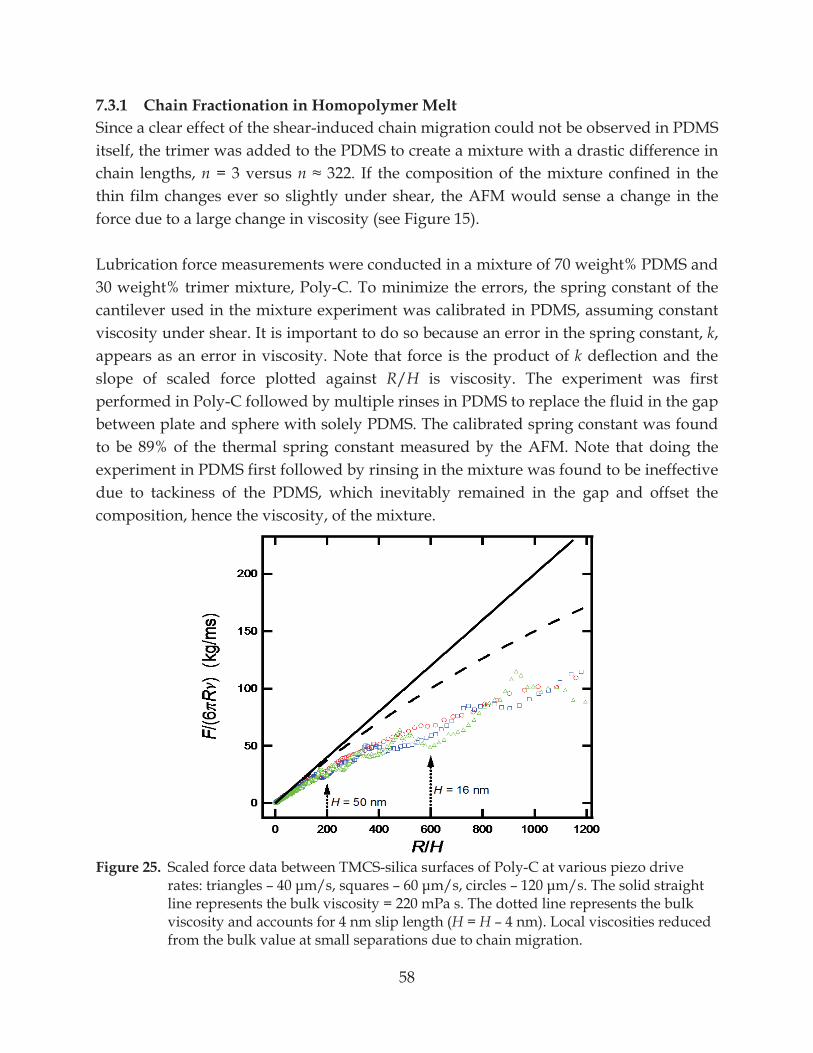
58

7.3.1 Chain Fractionation in Homopolymer Melt Since a clear effect of the shear-induced chain migration could not be observed in PDMSitself, the trimer was added to the PDMS to create a mixture with a drastic difference in chain lengths, n = 3 versus n thin film changes ever so slightly under shear, the AFM would sense a change in the force due to a large change in viscosity (see Figure 15). Lubrication force measurements were conducted in a mixture of 70 weight% PDMS and 30 weight% trimer mixture, Poly-C. To minimize the errors, the spring constant of the cantilever used in the mixture experiment was calibrated in PDMS, assuming constant viscosity under shear. It is important to do so because an error in the spring constant, k, appears as an error in viscosity. Note that force is the product of k deflection and the slope of scaled force plotted against R/H is viscosity. The experiment was first performed in Poly-C followed by multiple rinses in PDMS to replace the fluid in the gap between plate and sphere with solely PDMS. The calibrated spring constant was found to be 89% of the thermal spring constant measured by the AFM. Note that doing the experiment in PDMS first followed by rinsing in the mixture was found to be ineffective due to tackiness of the PDMS, which inevitably remained in the gap and offset the composition, hence the viscosity, of the mixture.

Figure 25. Scaled force data between TMCS-silica surfaces of Poly-C at various piezo drive

rates: triangles – s – – . The solid straight line represents the bulk viscosity = 220 mPa s. The dotted line represents the bulk viscosity and accounts for 4 nm slip length (H = H – 4 nm). Local viscosities reduced from the bulk value at small separations due to chain migration.

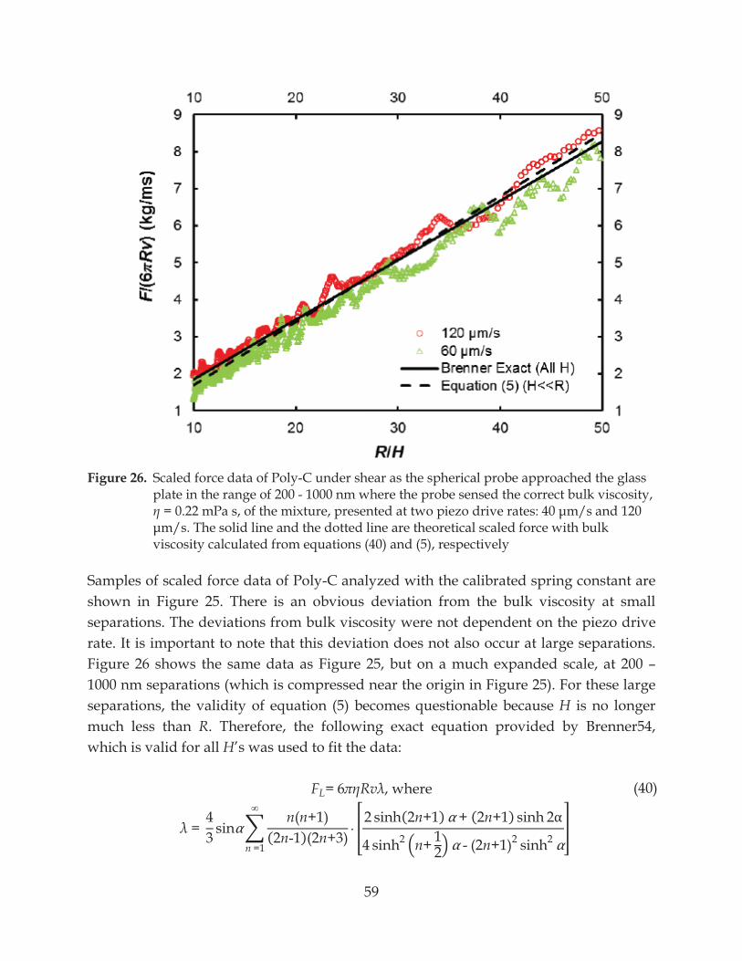
59

(40)

Figure 26. Scaled force data of Poly-C under shear as the spherical probe approached the glass

plate in the range of 200 - 1000 nm where the probe sensed the correct bulk viscosity,

viscosity calculated from equations (40) and (5), respectively Samples of scaled force data of Poly-C analyzed with the calibrated spring constant areshown in Figure 25. There is an obvious deviation from the bulk viscosity at smallseparations. The deviations from bulk viscosity were not dependent on the piezo driverate. It is important to note that this deviation does not also occur at large separations.Figure 26 shows the same data as Figure 25, but on a much expanded scale, at 200 –1000 nm separations (which is compressed near the origin in Figure 25). For these largeseparations, the validity of equation (5) becomes questionable because H is no longermuch less than R. Therefore, the following exact equation provided by Brenner54, which is valid for all H’s was used to fit the data:

FL= 6 Rv , where

= 43 sin

n(n+1)(2n-1)(2n+3)2 sinh(2n+1) + (2n+1) sinh 2

4 sinh2 n+ 12 - (2n+1)2 sinh2

n =1

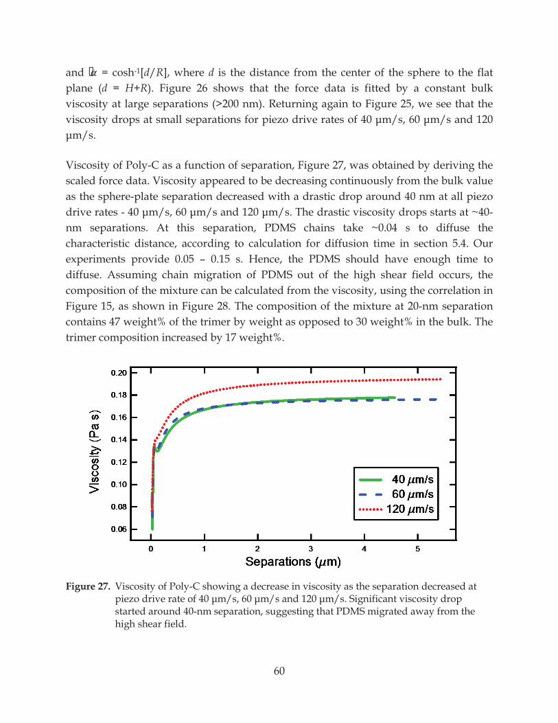
60

and = cosh-1[d/R], where d is the distance from the center of the sphere to the flatplane (d = H+R). Figure 26 shows that the force data is fitted by a constant bulk viscosity at large separations (>200 nm). Returning again to Figure 25, we see that the viscosity

Viscosity of Poly-C as a function of separation, Figure 27, was obtained by deriving the scaled force data. Viscosity appeared to be decreasing continuously from the bulk value as the sphere-plate separation decreased with a drastic drop around 40 nm at all piezo drive rates - 40 m/s, 60 m/s and 120 m/s. The drastic viscosity drops starts at ~40-nm separations. At this separation, PDMS chains take ~0.04 s to diffuse the characteristic distance, according to calculation for diffusion time in section 5.4. Our experiments provide 0.05 – 0.15 s. Hence, the PDMS should have enough time to diffuse. Assuming chain migration of PDMS out of the high shear field occurs, the composition of the mixture can be calculated from the viscosity, using the correlation in Figure 15, as shown in Figure 28. The composition of the mixture at 20-nm separationcontains 47 weight% of the trimer by weight as opposed to 30 weight% in the bulk. The trimer composition increased by 17 weight%.

Figure 27. Viscosity of Poly-C showing a decrease in viscosity as the separation decreased at piezo drive rate of 40 m/s, 60 m/s and 120 m/s. Significant viscosity drop started around 40-nm separation, suggesting that PDMS migrated away from the high shear field.

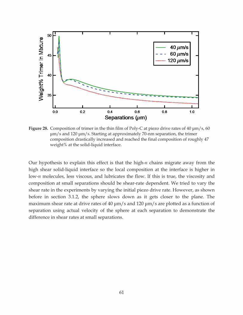
61

Figure 28. Composition of trimer in the thin film of Poly-C at piezo drive rates of 40 m/s, 60 m/s and 120 m/s. Starting at approximately 70-nm separation, the trimer

composition drastically increased and reached the final composition of roughly 47 weight% at the solid-liquid interface.

Our hypothesis to explain this effect is that the high-n chains migrate away from the high shear solid-liquid interface so the local composition at the interface is higher in low-n molecules, less viscous, and lubricates the flow. If this is true, the viscosity and composition at small separations should be shear-rate dependent. We tried to vary the shear rate in the experiments by varying the initial piezo drive rate. However, as shown before in section 3.1.2, the sphere slows down as it gets closer to the plane. The maximum shear rate separation using actual velocity of the sphere at each separation to demonstrate the difference in shear rates at small separations.

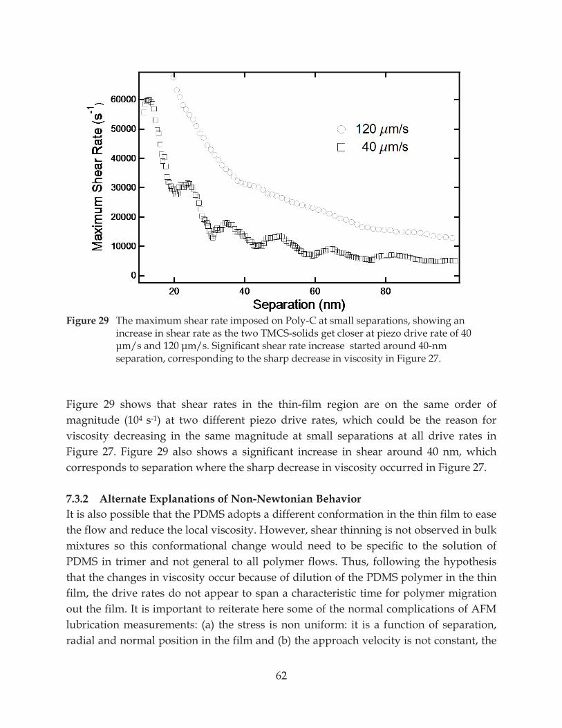
62

Figure 29 The maximum shear rate imposed on Poly-C at small separations, showing an

increase in shear rate as the two TMCS-solids get closer at piezo drive rate of 40 -nm

separation, corresponding to the sharp decrease in viscosity in Figure 27.

Figure 29 shows that shear rates in the thin-film region are on the same order of magnitude (104 s-1) at two different piezo drive rates, which could be the reason for viscosity decreasing in the same magnitude at small separations at all drive rates in Figure 27. Figure 29 also shows a significant increase in shear around 40 nm, which corresponds to separation where the sharp decrease in viscosity occurred in Figure 27. 7.3.2 Alternate Explanations of Non-Newtonian Behavior It is also possible that the PDMS adopts a different conformation in the thin film to ease the flow and reduce the local viscosity. However, shear thinning is not observed in bulk mixtures so this conformational change would need to be specific to the solution of PDMS in trimer and not general to all polymer flows. Thus, following the hypothesis that the changes in viscosity occur because of dilution of the PDMS polymer in the thin film, the drive rates do not appear to span a characteristic time for polymer migration out the film. It is important to reiterate here some of the normal complications of AFM lubrication measurements: (a) the stress is non uniform: it is a function of separation, radial and normal position in the film and (b) the approach velocity is not constant, the

63

sphere slows down at small separations due to the deflection of the cantilever under the lubrication force. (c) Due to such deceleration of the sphere, shear rates at small separations are not substantially different among different piezo drive rates. The reduced viscosity at small separations could have also been caused by a pre-existing concentration of the trimer at the solid-liquid interface. However, previous studies67-69 showed that in a shear-free environment a homopolymer melt containing molecules with different n, such as our PDMS-trimer melt, high-n molecules selectively adsorb to the solid surface. From such argument, if there were a pre-existing concentration of a type of molecules at the interface, it would be that of high-n molecules in PDMS and not the trimer. This argument is also supported by the comparison of the surface tension between PDMS on glass and trimer on glass in section 5.1, which found the surface tension of trimer to be 5.5 dyn/cm higher than that of PDMS on glass.

64

Chapter 8 CONCLUSION The work in this thesis shows that the assumption of the no-slip boundary condition is valid at hydrophilic and TMCS surfaces in polydimethylsiloxane (PDMS) of viscosities 0.82 – 970 mPa s under high shear up to 4×104 s-1 at piezo drive rate of 120 m/s. A mixture of PDMS and trimer exhibited Newtonian behavior at large separations (2000-5000 nm). Under high shear at small separations, the mixture of 70 weight% PDMS and 30 weight% octamethyltrisiloxane (trimer) showed a decrease in viscosity. When the measured viscosity was used to estimate the composition in the film at the solid liquid interface, the trimer composition at 20-nm separation was 47 weight%, increased from its initial content by 17 weight%. This dilution in PDMS concentration is not due to a pre-existing layer of trimer on glass surfaces as the surface tension of trimer on glass is higher than that of PDMS on glass as shown in section 5.1. The calculation of shear stress showed that the applied energy was much less than the required demixing energy calculated from the Flory-Huggins theory. The energy provided due to shear at 2.5×104 J/mole PDMS, which is less than the energy require to completely demix PDMS and trimer, -1.27×105 J/mole PDMS, although may be adequate to drive the partial demixing that we observed (3.9×104 J/mole PDMS required to increase the trimer concentration in the mixture by 17 weight%). The capillary flow between sphere and plane has a gradient in shear (see Figure 8), which is highest at solid-liquid interfaces and lowest at the midpoint between sphere and plane; this gradient in shear was shown to be the cause of chain migration by Shelby and Caflisch2, Horn et al35, and Cohen and Metzner73 in experiments which they found a lubrication layer at solid-liquid interfaces at the same or lower shear rates utilized in this thesis. Since PDMS is not shear-thinning, the decrease in viscosity can be attributed to the migration of long PMDS chains out of the high shear to remain in its entropically favorable coiled formation rather than stretching out with the flow as previously predicted by Tirrell and Malone1, Aubert and Tirrell71 and Ma and Graham72.

At low piezo drive rates, 100 – 1000 nm/s, where lubrication force is absent, strong capillary effect was detected on hydrophilic glass surfaces. This is consistent with the presence of water films on hydrophilic surfaces. Hydrophobizing the surface by TMCS vapor deposition diminished the capillary effect. In high speed runs, the capillary effect created difficulty in identifying zero separation and induced an error in lubrication analysis, which manifested in high standard deviations compared to data obtained on TMCS surfaces. We found that the presence of a thin lubricating film of low viscosity ( f ~1 mPa s and b ~ 1000 mPa s) did not have a large effect on the lubrication force. Specifically, the force did not follow the expected reduction due to a predicted slip

65

length of equation (9). All the reported slip lengths were within the combined roughness of the surfaces so we concluded that no slip was found.

66

Chapter 9 FUTURE RESEARCH 9.1 IMPROVE POLYDISPERSITY OF POLYMERS There was a range of chain sizes in our PDMS, and even though it did not greatly affect the outcome, the credibility of the result would be greatly improved if the PDMS has PDI Figure 24, which what we think is chain migration of longer PDMS chains out of the high-shear regime. A suggestion for an experiment to identify the mechanism of the migration is to use monodisperse polymers with different n’s. This would allow the effect of the difference in to be observed. 9.2 LOWER GIBB’S FREE ENERGY OF MIXING The calculation in section 5.3 shows that the Gibb’s free energy of mixing of our PDMS-OMTS mixture is very large compared to theoretical energy in which our shearing induced, section 3.1.2. In theory, the PDMS-OMTS mixture is very well-mixed. The next step would be to find a homopolymer melt with Gibb’s free energy of mixing on the same order of magnitude as the energy that the shear via AFM can induce ~102–103 s-1 and repeat the experiment in such polymer. 9.3 WIDEN THE RANGE OF SHEAR RATE We performed experiments between shear rates of 40 – 120 m/s using only one type of cantilever. Future research could use a few types of cantilevers with a range of spring constant to widen the range of shear rate in hope of finding the effect of shear on chain migration as observed in Horn et al35.

67

References

1. Tirrell, M.; Malone, M. F., Stress-Induced Diffusion of Macromolecules. Journal of Polymer Science Part B-Polymer Physics 1977, 15, (9), 1569-1583. 2. Shelby, M. D.; Caflisch, G. B., Shear field induced diffusion and molecular weight fractionation during polymer processing. Polymer Engineering & Science 2004, 44, (7), 1283-1294. 3. Lo, H. H.-K.; Chan, C.-M.; Zhu, S.-H., Characterization of the lubricant layer formed at the interface between the extrudate and the die wall during the extrusion of high density polyethylene and fluoroelastomer blends by XPS, SIMS and SEM. Polymer Engineering & Science 1999, 39, (4), 721-732. 4. Lee, H.; Archer, L. A., Functionalizing polymer surfaces by field-induced migration of copolymer additives—role of shear fields. Polymer Engineering & Science 2002, 42, (7), 1568-1579. 5. Bird, R. B.; Stewart, W. E.; Lightfoot, E. N., Transport phenomena. 2nd, Wiley international ed.; J. Wiley: New York, 2002; p xii, 895 p. 6. Craig, V. S.; Neto, C.; Williams, D. R., Shear-dependent boundary slip in an aqueous Newtonian liquid. Phys Rev Lett 2001, 87, (5), 054504. 7. Neto, C.; Craig, V. S.; Williams, D. R., Evidence of shear-dependent boundary slip in newtonian liquids. Eur Phys J E Soft Matter 2003, 12 Suppl 1, 71-4. 8. Honig, C. D. F.; Ducker, W. A., Squeeze Film Lubrication in Silicone Oil: Experimental Test of the No-Slip Boundary Condition at Solid−Liquid Interfaces. The Journal of Physical Chemistry C 2008, 112, (44), 17324-17330. 9. Vinogradova, O. I., Drainage of a Thin Liquid Film Confined between Hydrophobic Surfaces. Langmuir 1995, 11, (6), 2213-2220. 10. Bernoulli, D.; Pre-1801 Imprint Collection (Library of Congress), Danielis Bernoulli ... Hydrodynamica, sive De viribus et motibus fluidorum commentarii. sumptibus J. R. Dulseckeri: Argentorati,, 1738; p 4 p. 11. Stokes, G. G., Trans. Cambridge Phil. Soc. 1845, 3, 287. 12. Stokes, G. G., On the effect of the internal friction of fluids on the motion of pendulums. Pitt Press: Cambridge, 1851. 13. Coulomb, C. A., Memoires de l'Institut National des Sciences et des Arts: Sciences Mathematiques et Physiques 1801, 3. 14. Warburg, E. G., Poggendorff's Annalen 1870, 140, 367. 15. Couette, M., Etudes sur le frottement des liquides. Ann. Chim. Phys. 1890, 21, 433. 16. Girard, P. S., Mémoires de la Classe des Sciences Mathématiques et Physiques de l'Institut de France. 1815, 329. 17. Ruckenstein, E.; Rajora, P., On the no-slip boundary condition of hydrodynamics. J. Colloid Interface Sci. 1983, 96, (2), 488. 18. Navier, C., Mémoire sur les lois du mouvement des fluids. Mem. Acad. Sci. Inst. Fr. 1823, 6, 389. 19. Helmholtz, H. v.; Piotrowski, G. v., Über reibung tropfbarer flussigkeiten. Sitzungsberichte der Kaiserlich Akademie der Wissenschaften (Wien) 1860, 40, 607. 20. Poiseuille, J., Recherches sur les causes du mouvement du sang dans les vaisseaux capillaires. 1841. 21. Ladenburg, R., Über den Einfluß der Reibung auf die Schwingungen einer mit Flüssigkeit gefüllten Kugel. Ann. Phys. 1907, 328, (8), 447. 22. Tretheway, D. C.; Meinhart, C. D., Apparent fluid slip at hydrophobic microchannel walls. Phys. Fluids 2002, 14, (3), L9.

68

23. Tretheway, D. C.; Meinhart, C. D., A generating mechanism for apparent fluid slip in hydrophobic microchannels. Phys. Fluids 2004, 16, (5), 1509. 24. Joseph, P.; Tabeling, P., Direct measurement of the apparent slip length. Physical Review E 2005, 71, (3), 035303. 25. Joly, L.; Ybert, C.; Bocquet, L., Probing the nanohydrodynamics at liquid-solid interfaces using thermal motion. 2005. 26. Zettner; Yoda, Particle velocity field measurements in a near-wall flow using evanescent wave illumination. Experiments in Fluids 2003, 34, (1), 115-121. 27. Huang, P.; Breuer, K. S., Direct measurement of slip length in electrolyte solutions. Physics of Fluids 2007, 19, (2), 028104. 28. Li, H.; Sadr, R.; Yoda, M., Multilayer nano-particle image velocimetry. Experiments in Fluids 2006, 41, (2), 185-194. 29. Ulmanella, U.; Ho, C.-M., Molecular effects on boundary condition in micro/nanoliquid flows. Physics of Fluids 2008, 20, (10), 101512. 30. Choi, C.-H.; Westin, J. A.; Breuer, K. S., Apparent slip flows in hydrophilic and hydrophobic microchannels. Phys. Fluids 2003, 15, (10), 2897. 31. Cheng, J. T.; Giordano, N., Fluid flow through nanometer-scale channels. Phys. Rev. 2002, 65, (3), 031206. 32. Israelachvili, J. N.; Tabor, D., The measurement of van der Waals dispersion forces in the range 1.5 to 130 nm. Proc. R. Soc. Lond. 1972, 331, (1584), 19. 33. Zhu, Y.; Granick, S., Rate-dependent slip of Newtonian liquids at smooth surfaces. Phys. Rev. Lett. 2001, 87, 96105. 34. Zhu, Y.; Granick, S., Limits of the hydrodynamic no-slip boundary condition. Phys. Rev. Lett. 2002, 88, (10), 106102. 35. Horn, R. G.; Vinogradova, O. I.; Mackay, M. E.; Phan-Thien, N., Hydrodynamic slippage inferred from thin film drainage measurements in a solution of nonadsorbing polymer. J. Chem. Phys. 2000, 112, (14), 6424. 36. Baudry, J.; Charlaix, E.; Tonck, A.; Mazuyer, D., Experimental evidence for a large slip effect at a nonwetting fluid-solid interface. Langmuir 2001, 17, (17), 5232. 37. Cottin-Bizonne, C.; Cross, B.; Steinberger, A.; Charlaix, E., Boundary slip on smooth hydrophobic surfaces: intrinsic effects and possible artefacts. Phys. Rev. Lett. 2005, 94, (5), 056102. 38. Cottin-Bizonne, C.; Steinberger, A.; Cross, B.; Raccurt, O.; Charlaix, E., Nanohydrodynamics: The Intrinsic Flow Boundary Condition on Smooth Surfaces. Langmuir 2008, 24, (4), 1165-1172. 39. Steinberger, A.; Cottin-Bizonne, C.; Kleimann, P.; Charlaix, E., High friction on a bubble mattress. Nat Mater 2007, 6, (9), 665-668. 40. Adrian, R. J., Twenty years of particle image velocimetry. Experiments in Fluids 2005, 39, (2), 159-169. 41. Neto, C.; Evans, D. R.; Bonaccurso, E.; Butt, H.-J.; Craig, V. S. J., Boundary slip in Newtonian liquids: a review of experimental studies. Reports on Progress in Physics 2005, (12), 2859. 42. Pouya, S.; Koochesfahani, M.; Snee, P.; Bawendi, M.; Nocera, D., Single quantum dot (QD) imaging of fluid flow near surfaces. Experiments in Fluids 2005, 39, (4), 784-786. 43. Lauga E, B. M. P., Stone H A, Handbook of Experimental Fluid Dynamics 2005.

69

44. Lumma, D.; Best, A.; Gansen, A.; Feuillebois, F.; auml; dler, J. O.; Vinogradova, O. I., Flow profile near a wall measured by double-focus fluorescence cross-correlation. Physical Review E 2003, 67, (5), 056313. 45. Baek, S. J.; Lee, S. J., A new two-frame particle tracking algorithm using match probability. Experiments in Fluids 1996, 22, (1), 23-32. 46. Ou, J.; Perot, B.; Rothstein, J. P., Laminar drag reduction in microchannels using ultrahydrophobic surfaces. Physics of Fluids 2004, 16, (12), 4635-4643. 47. Ou, J.; Rothstein, J. P., Direct velocity measurements of the flow past drag-reducing ultrahydrophobic surfaces. Physics of Fluids 2005, 17, (10), 103606. 48. Majumder, M.; Chopra, N.; Andrews, R.; Hinds, B. J., Nanoscale hydrodynamics: Enhanced flow in carbon nanotubes. Nature 2005, 438, (7064), 44-44. 49. Chan, D. Y. C.; Horn, R. G., The drainage of thin liquid films between solid surfaces. J. Chem. Phys. 1985, 83, (10), 5311. 50. Bhushan, B., Springer handbook of nanotechnology. In Springer: Berlin; New York, 2004; pp 863-865. 51. Lin, Z.; Granick, S., Platinum Nanoparticles at Mica Surfaces. Langmuir 2003, 19, (17), 7061-7070. 52. Israelachvili, J. N.; Alcantar, N. A.; Maeda, N.; Mates, T. E.; Ruths, M., Preparing contamination-free mica substrates for surface characterisation, force measurements and imaging. Langmuir 2004, 20, (9), 3616. 53. Ducker, W. A.; Senden, T. J.; Pashley, R. M., Direct Measurement of Colloidal Forces Using an Atomic Force Microscope. Nature 1991, 353, (6341), 239-241. 54. Brenner, H., The slow motion of a sphere through a viscous fluid towards a plane surface. Chem. Engng. Sci. 1961, 16, 242-251. 55. McBride, S. P.; Law, B. M., Improved in situ spring constant calibration for colloidal probe atomic force microscopy. Review of Scientific Instruments 81, (11), 113703. 56. Honig, C. D.; Ducker, W. A., No-slip hydrodynamic boundary condition for hydrophilic particles. Phys Rev Lett 2007, 98, (2), 028305. 57. Henry, C. L.; Craig, V. S. J., Measurement of no-slip and slip boundary conditions in confined Newtonian fluids using atomic force microscopy. Physical Chemistry Chemical Physics 2009, 11, (41), 9514-9521. 58. Guillot, P.; Panizza, P.; Salmon, J. B.; Joanicot, M.; Colin, A.; Bruneau, C. H.; Colin, T., Viscosimeter on a microfluidic chip. Langmuir 2006, 22, (14), 6438-6445. 59. Thompson, P. A., A general boundary condition for liquid flow at solid surfaces. The Astrophysical journal 1983, 271, 283. 60. Seyferth, D., Dimethyldichlorosilane and the Direct Synthesis of Methylchlorosilanes. The Key to the Silicones Industry†Organometallics 2001, 20, (24), 4978-4992. 61. Rochow, E. G., The Direct Synthesis of Organosilicon Compounds. Journal of the American Chemical Society 1945, 67, (6), 963-965. 62. Kipping, F. S., Organic derivative of silicon. Preparation of alkylsilicon chlorides. Proceedings of the Chemical Society 1904, 20, 15. 63. Barrére, M.; Capitao da Silva, S.; Balic, R.; Ganachaud, F. o., Synthesis of Monodisperse Poly(dimethylsiloxane) Micro- and Macroemulsions. Langmuir 2001, 18, (3), 941-944. 64. Mills, N. J., The rheological properties and molecular weight distribution of polydimethylsiloxane. European Polymer Journal 1969, 5, (5), 675-695. 65. Johnson, G. C., Flow Characteristics of Linear, End-Blocked Dimethylpolysiloxane Fluids. Journal of Chemical & Engineering Data 1961, 6, (2), 275-278.

70

66. Dvornic, P. R.; Jovanovic, J. D.; Govedarica, M. N., On the critical molecular chain length of polydimethylsiloxane. Journal of Applied Polymer Science 1993, 49, (9), 1497-1507. 67. Dijt, J. C.; Cohen Stuart, M. A.; Fleer, G. J., Competitive Adsorption Kinetics of Polymers Differing in Length Only. Macromolecules 1994, 27, (12), 3219-3228. 68. Scheutjens, J. M. H. M.; Fleer, G. J.; Tadros, T. F., The Effects of Polymer on Dispersion Properties. Academic Press: London 1982. 69. Santore, M.; Fu, Z., Direct Measurement of Molecular-Weight Driven Competition during Polymer Adsorption. Macromolecules 1997, 30, (26), 8516-8517. 70. Jalbert, C.; Koberstein, J. T.; Yilgor, I.; Gallagher, P.; Krukonis, V., Molecular weight dependence and end-group effects on the surface tension of poly(dimethylsiloxane). Macromolecules 1993, 26, (12), 3069-3074. 71. Aubert, J. H.; Tirrell, M., Macromolecules in nonhomogeneous velocity gradient fields. The Journal of Chemical Physics 1980, 72, (4), 2694-2701. 72. Ma, H.; Graham, M. D., Theory of shear-induced migration in dilute polymer solutions near solid boundaries. Physics of Fluids 2005, 17, (8), 083103. 73. Cohen, Y.; Metzner, A. B., Apparent Slip Flow of Polymer Solutions. Journal of Rheology 1985, 29, (1), 67-102. 74. Flory, P. J., Thermodynamics of High Polymer Solutions. The Journal of Chemical Physics 1941, 9, (8), 660-660. 75. Huggins, M. L., Solutions of Long Chain Compounds. The Journal of Chemical Physics 1941, 9, (5), 440-440. 76. Prausnitz, J. M.; Lichtenthaler, R. N.; Azevedo, E. G. d., Molecular thermodynamics of fluid-phase equilibria. Prentice Hall PTR: Upper Saddle River, N.J., 1999. 77. Chan, D. Y. C.; Horn, R. G., The Drainage of Thin Liquid-Films between Solid-Surfaces. Journal of Chemical Physics 1985, 83, (10), 5311-5324. 78. Appel, M.; Fleischer, G., Investigation of the chain length dependence of self-diffusion of poly(dimethylsiloxane) and poly(ethylene oxide) in the melt with pulsed field gradient NMR. Macromolecules 1993, 26, (20), 5520-5525. 79. Sader, J. E.; Chon, J. W. M.; Mulvaney, P., Calibration of rectangular atomic force microscope cantilevers. Review of Scientific Instruments 1999, 70, (10), 3967-3969. 80. Xiao, X.; Qian, L., Investigation of Humidity-Dependent Capillary Force. Langmuir 2000, 16, (21), 8153-8158. 81. Orr, F. M.; Scriven, L. E.; Rivas, A. P., Pendular rings between solids: meniscus properties and capillary force. Journal of Fluid Mechanics 1975, 67, (04), 723-742.