lrfd steel design.pdf
TRANSCRIPT

7/29/2019 LRFD steel design.pdf
http://slidepdf.com/reader/full/lrfd-steel-designpdf 1/646
December 2003
FHWA NHI-04-0LRFD Design Examplefor
Steel Girder Superstructure Bridge
Prepared for
FHWA / National Highway Institute
Washington, DC
US UnitsPrepared by
Michael Baker Jr In
Moon Township, Pennsylvania

7/29/2019 LRFD steel design.pdf
http://slidepdf.com/reader/full/lrfd-steel-designpdf 2/646
Development of a Comprehensive Design
Example for a Steel Girder Bridge
with Commentary
Design Process Flowcharts for
Superstructure and Substructure Designs
Prepared by
Michael Baker Jr., Inc.
November 2003
7/29/2019 LRFD steel design.pdf
http://slidepdf.com/reader/full/lrfd-steel-designpdf 3/646
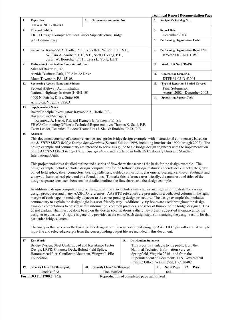
Technical Report Documentation Page
1. Report No. 2. Government Accession No. 3. Recipient’s Catalog No.
FHWA NHI - 04-041
4. Title and Subtitle 5. Report Date
LRFD Design Example for Steel Girder Superstructure Bridge December 2003
with Commentary 6. Performing Organization Code
7. Author (s) Raymond A. Hartle, P.E., Kenneth E. Wilson, P.E., S.E., 8. Performing Organization Report No.
William A. Amrhein, P.E., S.E., Scott D. Zang, P.E.,Justin W. Bouscher, E.I.T., Laura E. Volle, E.I.T.
B25285 001 0200 HRS
9. Performing Organization Name and Address 10. Work Unit No. (TRAIS)
Michael Baker Jr., Inc.
Airside Business Park, 100 Airside Drive 11. Contract or Grant No.
Moon Township, PA 15108 DTFH61-02-D-63001
12. Sponsoring Agency Name and Address 13. Type of Report and Period Covered
Federal Highway Administration Final Submission National Highway Institute (HNHI-10) August 2002 - December 2003
4600 N. Fairfax Drive, Suite 800 14. Sponsoring Agency Code
Arlington, Virginia 22203
15. Supplementary Notes
Baker Principle Investigator: Raymond A. Hartle, P.E.Baker Project Managers:
Raymond A. Hartle, P.E. and Kenneth E. Wilson, P.E., S.E.
FHWA Contracting Officer’s Technical Representative: Thomas K. Saad, P.E.Team Leader, Technical Review Team: Firas I. Sheikh Ibrahim, Ph.D., P.E.
16. Abstract
This document consists of a comprehensive steel girder bridge design example, with instructional commentary based on
the AASHTO LRFD Bridge Design Specifications(Second Edition, 1998, including interims for 1999 through 2002). The
design example and commentary are intended to serve as a guide to aid bridge design engineers with the implementationof the AASHTO LRFD Bridge Design Specifications, and is offered in both US Customary Units and Standard
International Units.
This project includes a detailed outline and a series of flowcharts that serve as the basis for the design example. The
design example includes detailed design computations for the following bridge features: concrete deck, steel plate girder, bolted field splice, shear connectors, bearing stiffeners, welded connections, elastomeric bearing, cantilever abutment and wingwall, hammerhead pier, and pile foundations. To make this reference user-friendly, the numbers and titles of the
design steps are consistent between the detailed outline, the flowcharts, and the design example.
In addition to design computations, the design example also includes many tables and figures to illustrate the various
design procedures and many AASHTO references. AASHTO references are presented in a dedicated column in the rightmargin of each page, immediately adjacent to the corresponding design procedure. The design example also includes
commentary to explain the design logic in a user-friendly way. Additionally, tip boxes are used throughout the design
example computations to present useful information, common practices, and rules of thumb for the bridge designer. Tipsdo not explain what must be done based on the design specifications; rather, they present suggested alternatives for the
designer to consider. A figure is generally provided at the end of each design step, summarizing the design results for that
particular bridge element.
The analysis that served as the basis for this design example was performed using the AASHTO Opis software. A sample
input file and selected excerpts from the corresponding output file are included in this document.
17. Key Words 18. Distribution Statement
Bridge Design, Steel Girder, Load and Resistance Factor This report is available to the public from the
Design, LRFD, Concrete Deck, Bolted Field Splice, National Technical Information Service in
Hammerhead Pier, Cantilever Abutment, Wingwall, Pile Springfield, Virginia 22161 and from the
Foundation Superintendent of Documents, U.S. GovernmentPrinting Office, Washington, D.C. 20402.
19. Security Classif. (of this report) 20. Security Classif. (of this page) 21. No. of Pages 22. Price
Unclassified Unclassified 644
Form DOT F 1700.7 (8-72) Reproduction of completed page authorized

7/29/2019 LRFD steel design.pdf
http://slidepdf.com/reader/full/lrfd-steel-designpdf 4/646
This page intentionally left blank

7/29/2019 LRFD steel design.pdf
http://slidepdf.com/reader/full/lrfd-steel-designpdf 5/646
ACKNOWLEDGEMENTS
We would like to express appreciation to the Illinois Department of Transportation, Washington State Department of Transportation, and Mr. Mike Grubb, BSDI, for providing expertise on the Technical Review Committee.
We would also like to acknowledge the contributions of the following staff members at Michael Baker Jr., Inc.:
Tracey A. AndersonJeffrey J. Campbell, P.E.
James A. Duray, P.E.John A. Dziubek, P.E.David J. Foremsky, P.E.Maureen KanfoushHerman Lee, P.E.
Joseph R. McKool, P.E.Linda MontagnaV. Nagaraj, P.E.Jorge M. Suarez, P.E.
Scott D. Vannoy, P.E.Roy R. WeilRuth J. Williams

7/29/2019 LRFD steel design.pdf
http://slidepdf.com/reader/full/lrfd-steel-designpdf 6/646
Table of Contents
1. Flowcharting Conventions
Chart 3 - Steel Girder Design
Chart 2 - Concrete Deck Design
Chart 1 - General Information
2. Flowcharts
Chart 6 - Bearing Design
Main Flowchart
Chart 4 - Bolted Field Splice Design
Chart P - Pile Foundation Design
Chart 8 - Pier Design
Chart 7 - Abutment and Wingwall Design
Chart 5 - Miscellaneous Steel Design

7/29/2019 LRFD steel design.pdf
http://slidepdf.com/reader/full/lrfd-steel-designpdf 7/646
Flowcharting Conventions
Decision
Commentary to provide
additional information
about the decision or
process.
Flowchart reference or
article in AASHTO LRFD
Bridge Design Specifications
YesNo
A process may have an entry
point from more than one path.
An arrowhead going into a
process signifies an entry point.
Unless the process is adecision, there is only
one exit point.
A line going out of a
process signifies an exit
point.
Unique sequence
identifier
Process description
Process
Chart # or AASHTO Reference
Design
Step #
Process
Chart # or
AASHTO Reference
Design
Step #
A
Reference
Supplemental
Information
Start
Go to Other
Flowchart
Flowcharts Design Example for a Two-Span Brid
FHWA LRFD Steel Design Example
7/29/2019 LRFD steel design.pdf
http://slidepdf.com/reader/full/lrfd-steel-designpdf 8/646
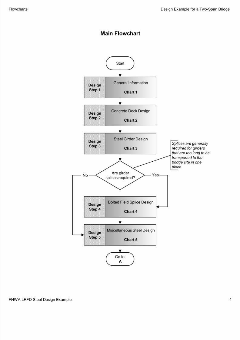
Main Flowchart
Are girder
splices required?
Splices are generally
required for girders
that are too long to be
transported to the
bridge site in one
piece.
General Information
Chart 1
Design
Step 1
Bolted Field Splice Design
Chart 4
Design
Step 4
Concrete Deck Design
Chart 2
Design
Step 2
Steel Girder Design
Chart 3
Design
Step 3
No Yes
Miscellaneous Steel Design
Chart 5
Design
Step 5
Start
Go to:
A
Flowcharts Design Example for a Two-Span Brid
FHWA LRFD Steel Design Example

7/29/2019 LRFD steel design.pdf
http://slidepdf.com/reader/full/lrfd-steel-designpdf 9/646
Main Flowchart (Continued)
Bearing Design
Chart 6
Design
Step 6
Miscellaneous Design
Chart 9
Design
Step 9
Abutment and
Wingwall Design
Chart 7
Design
Step 7
Pier Design
Chart 8
Design
Step 8
Special Provisions
and Cost Estimate
Chart 10
Design
Step 10
Design
Completed
A
Note:
Design Step P is used for pile foundation
design for the abutments, wingwalls, or piers.
Flowcharts Design Example for a Two-Span Brid
FHWA LRFD Steel Design Example

7/29/2019 LRFD steel design.pdf
http://slidepdf.com/reader/full/lrfd-steel-designpdf 10/646
General Information Flowchart
Are girder
splices
required?
Bolted Field Splice
Design
Chart 4
Design
Step 4
Steel Girder Design
Chart 3
Design
Step 3
No Yes
Miscellaneous Steel
Design
Chart 5
Design
Step 5
Design
Completed
Bearing Design
Chart 6
Design
Step 6
Miscellaneous
Design
Chart 9
Design
Step 9
Abutment and
Wingwall Design
Chart 7
Design
Step 7
Pier Design
Chart 8
Design
Step 8
Special Provisions
and Cost Estimate
Chart 10
Design
Step
10
Start
Concrete Deck
Design
Chart 2
Design
Step 2
General Information
Chart 1
Design
Step 1
Includes:
Governing
specifications, codes,
and standards
Design methodology
Live load requirements
Bridge width
requirements
Clearance
requirements
Bridge length
requirements
Material propertiesFuture wearing surface
Load modifiers
Start
Obtain Design CriteriaDesign
Step 1.1
Includes:
Horizontal curve data
and alignment
Vertical curve data and
grades
Obtain Geometry
Requirements
Design
Step 1.2
Go to:
A
Perform Span
Arrangement Study
Design
Step 1.3
Does client
require a Span
Arrangement
Study?
Select Bridge Type and
Develop Span Arrangement
Design
Step 1.3
Includes:
Select bridge type
Determine span
arrangement
Determine substructure
locations
Compute span lengths
Check horizontal
clearance
NoYes
Chart 1
Flowcharts Design Example for a Two-Span Brid
FHWA LRFD Steel Design Example

7/29/2019 LRFD steel design.pdf
http://slidepdf.com/reader/full/lrfd-steel-designpdf 11/646
General Information Flowchart (Continued)
Includes:
Boring logs
Foundation type
recommendations for
all substructures
Allowable bearing
pressure
Allowable settlement
Overturning
Sliding
Allowable pile
resistance (axial and
lateral)
Are girder
splices
required?
Bolted Field Splice
Design
Chart 4
Design
Step 4
Steel Girder Design
Chart 3
Design
Step 3
No Yes
Miscellaneous Steel
Design
Chart 5
DesignStep 5
Design
Completed
Bearing Design
Chart 6
Design
Step 6
Miscellaneous
Design
Chart 9
Design
Step 9
Abutment and
Wingwall Design
Chart 7
Design
Step 7
Pier Design
Chart 8
Design
Step 8
Special Provisions
and Cost Estimate
Chart 10
Design
Step
10
Start
Concrete Deck
Design
Chart 2
Design
Step 2
General InformationChart 1
DesignStep 1
Obtain Geotechnical
Recommendations
Design
Step 1.4
A
Perform Type, Size
and Location Study
Design
Step 1.5
Does client
require a Type,
Size and Location
Study?
Determine Optimum
Girder Configuration
Design
Step 1.5
Includes:
Select steel girder
types
Girder spacing
Approximate girder
depth
Check vertical
clearance
NoYes
Return to
Main Flowchart
Plan for Bridge Aesthetics
S2.5.5
Design
Step 1.6
Considerations include:Function
Proportion
Harmony
Order and rhythm
Contrast and texture
Light and shadow
Chart 1
Flowcharts Design Example for a Two-Span Brid
FHWA LRFD Steel Design Example
7/29/2019 LRFD steel design.pdf
http://slidepdf.com/reader/full/lrfd-steel-designpdf 12/646
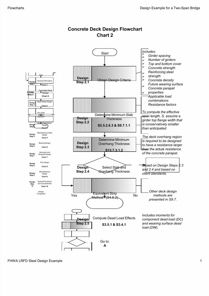
Concrete Deck Design Flowchart
Equivalent Strip
Method? (S4.6.2)
Includes:Girder spacing
Number of girders
Top and bottom cover
Concrete strength
Reinforcing steel
strength
Concrete density
Future wearing surface
Concrete parapet
properties
Applicable load
combinations
Resistance factors
Start
Go to:
A
Obtain Design CriteriaDesign
Step 2.1
Select Slab and
Overhang Thickness
Design
Step 2.4
Determine Minimum Slab
Thickness
S2.5.2.6.3 & S9.7.1.1
Design
Step 2.2
Determine Minimum
Overhang Thickness
S13.7.3.1.2
Design
Step 2.3
Compute Dead Load Effects
S3.5.1 & S3.4.1
Design
Step 2.5
To compute the effective
span length, S, assume a
girder top flange width that
is conservatively smaller
than anticipated.
NoYes
Based on Design Steps 2.3
and 2.4 and based on
client standards.
The deck overhang region
is required to be designed
to have a resistance larger
than the actual resistance
of the concrete parapet.
Other deck designmethods are
presented in S9.7.
Are girder
splices
required?
Bolted Field Splice
Design
Chart 4
Design
Step 4
Concrete Deck
Design
Chart 2
Design
Step 2
Steel Girder Design
Chart 3
Design
Step 3
No Yes
Miscellaneous Steel
Design
Chart 5
Design
Step 5
Design
Completed
Bearing Design
Chart 6
Design
Step 6
Miscellaneous
Design
Chart 9
Design
Step 9
Abutment and
Wingwall Design
Chart 7
Design
Step 7
Pier Design
Chart 8
Design
Step 8
Special Provisions
and Cost Estimate
Chart 10
Design
Step
10
Start
General Information
Chart 1
Design
Step 1
Includes moments for
component dead load (DC)
and wearing surface dead
load (DW).
Chart 2
Flowcharts Design Example for a Two-Span Brid
FHWA LRFD Steel Design Example
7/29/2019 LRFD steel design.pdf
http://slidepdf.com/reader/full/lrfd-steel-designpdf 13/646
Concrete Deck Design Flowchart (Continued)
Are girder
splices
required?
Bolted Field Splice
Design
Chart 4
Design
Step 4
Concrete Deck
Design
Chart 2
Design
Step 2
Steel Girder Design
Chart 3
Design
Step 3
No Yes
Miscellaneous Steel
Design
Chart 5
Design
Step 5
Design
Completed
Bearing Design
Chart 6
Design
Step 6
Miscellaneous
Design
Chart 9
Design
Step 9
Abutment and
Wingwall Design
Chart 7
Design
Step 7
Pier Design
Chart 8
Design
Step 8
Special Provisions
and Cost Estimate
Chart 10
Design
Step
10
Start
General Information
Chart 1
Design
Step 1
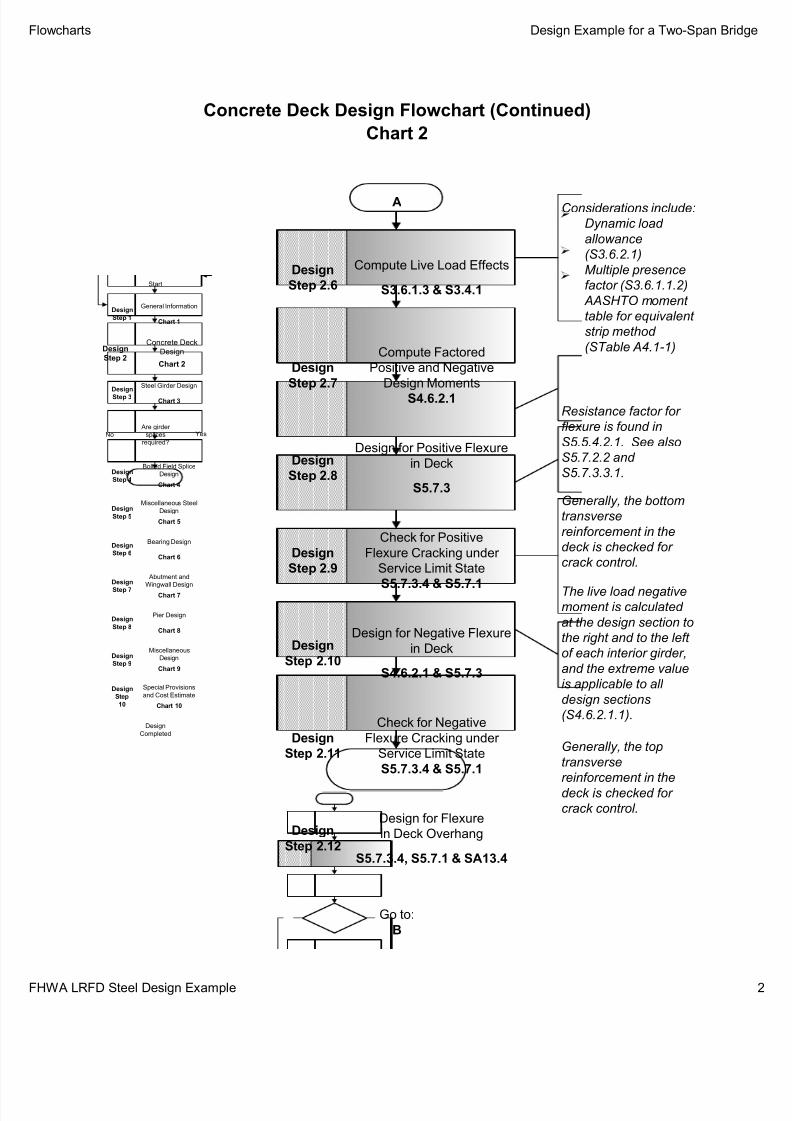
Compute Factored
Positive and Negative
Design Moments
S4.6.2.1
Design
Step 2.7
Design for Negative Flexure
in Deck
S4.6.2.1 & S5.7.3
Design
Step 2.10
Design for Positive Flexure
in Deck
S5.7.3
Design
Step 2.8
Check for Positive
Flexure Cracking under
Service Limit State
S5.7.3.4 & S5.7.1
Design
Step 2.9
Resistance factor for
flexure is found in
S5.5.4.2.1. See also
S5.7.2.2 and
S5.7.3.3.1.
Generally, the bottom
transverse
reinforcement in the
deck is checked for
crack control.
The live load negativemoment is calculated
at the design section to
the right and to the left
of each interior girder,
and the extreme value
is applicable to all
design sections
(S4.6.2.1.1).Check for Negative
Flexure Cracking under
Service Limit State
S5.7.3.4 & S5.7.1
Design
Step 2.11Generally, the top
transverse
reinforcement in the
deck is checked for
crack control.Design for Flexure
in Deck Overhang
S5.7.3.4, S5.7.1 & SA13.4
Design
Step 2.12
Go to:
B
A
Compute Live Load Effects
S3.6.1.3 & S3.4.1
Design
Step 2.6
Considerations include:
Dynamic load
allowance
(S3.6.2.1)
Multiple presence
factor (S3.6.1.1.2)
AASHTO moment
table for equivalent
strip method
(STable A4.1-1)
Chart 2
Flowcharts Design Example for a Two-Span Brid
FHWA LRFD Steel Design Example

7/29/2019 LRFD steel design.pdf
http://slidepdf.com/reader/full/lrfd-steel-designpdf 14/646
Concrete Deck Design Flowchart (Continued)
Design Overhang
for
Vertical Collision
Force
SA13.4.1
Design
Case 2
Design Overhang
for
Dead Load and
Live Load
SA13.4.1
Design
Case 3
Design Overhang
for Horizontal
Vehicular Collision
Force
SA13.4.1
Design
Case 1
For concrete parapets,
the case of vertical collision never controls.
Check atDesign
Section in
First Span
Case
3B
Check atDesign
Section in
Overhang
Case
3A
Check atInside Face
of Parapet
Case
1A
Check atDesign
Section in
First Span
Case
1C
Check atDesign
Section in
Overhang
Case
1B
As(Overhang) =
maximum of the
above five
reinforcing steel
areas
Are girder
splices
required?
Bolted Field Splice
Design
Chart 4
Design
Step 4
Concrete Deck
Design
Chart 2
Design
Step 2
Steel Girder Design
Chart 3
Design
Step 3
No Yes
Miscellaneous Steel
Design
Chart 5
Design
Step 5
Design
Completed
Bearing Design
Chart 6
Design
Step 6
Miscellaneous
Design
Chart 9
Design
Step 9
Abutment and
Wingwall Design
Chart 7
DesignStep 7
Pier Design
Chart 8
Design
Step 8
Special Provisions
and Cost Estimate
Chart 10
Design
Step
10
Start
General Information
Chart 1
Design
Step 1
Go to:
C
Use As(Deck)
in overhang.
Use As(Overhang)
in overhang.
Check for Cracking
in Overhang under
Service Limit State
S5.7.3.4 & S5.7.1
Design
Step 2.13
Does not control
the design in
most cases.
Compute Overhang Cut-off
Length Requirement
S5.11.1.2
Design
Step 2.14
The overhang
reinforcing steel must satisfy both
the overhang
requirements
and the deck
requirements.
As(Overhang) >
As
(Deck)?Yes No
B
Chart 2
Flowcharts Design Example for a Two-Span Brid
FHWA LRFD Steel Design Example
7/29/2019 LRFD steel design.pdf
http://slidepdf.com/reader/full/lrfd-steel-designpdf 15/646
Concrete Deck Design Flowchart (Continued)
Are girder
splices
required?
Bolted Field Splice
Design
Chart 4
Design
Step 4
Concrete Deck
Design
Chart 2
Design
Step 2
Steel Girder Design
Chart 3
Design
Step 3
No Yes
Miscellaneous Steel
Design
Chart 5
Design
Step 5
Design
Completed
Bearing Design
Chart 6
Design
Step 6
Miscellaneous
Design
Chart 9
Design
Step 9
Abutment and
Wingwall Design
Chart 7
Design
Step 7
Pier Design
Chart 8
Design
Step 8
Special Provisions
and Cost Estimate
Chart 10
Design
Step
10
Start
General Information
Chart 1
Design
Step 1
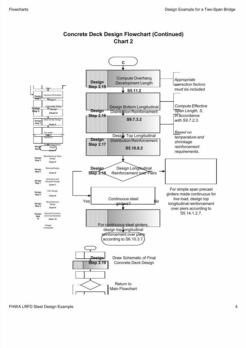
Compute Effective
Span Length, S,
in accordance
with S9.7.2.3.
Compute Overhang
Development Length
S5.11.2
Design
Step 2.15
Appropriate
correction factors
must be included.
Design Bottom Longitudinal
Distribution Reinforcement
S9.7.3.2
Design
Step 2.16
Return to
Main Flowchart
C
Design Longitudinal
Reinforcement over Piers
Design
Step 2.18
Continuous steel
girders?Yes No
For simple span precast
girders made continuous for
live load, design top
longitudinal reinforcement
over piers according to
S5.14.1.2.7.
For continuous steel girders,
design top longitudinal
reinforcement over piers
according to S6.10.3.7.
Design Top Longitudinal
Distribution Reinforcement
S5.10.8.2
Design
Step 2.17
Based on
temperature and
shrinkage
reinforcement
requirements.
Draw Schematic of Final
Concrete Deck Design
Design
Step 2.19
Chart 2
Flowcharts Design Example for a Two-Span Brid
FHWA LRFD Steel Design Example
7/29/2019 LRFD steel design.pdf
http://slidepdf.com/reader/full/lrfd-steel-designpdf 16/646
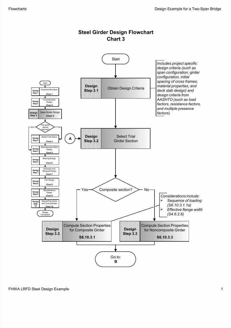
Steel Girder Design Flowchart
Includes project specific
design criteria (such as
span configuration, girder
configuration, initial
spacing of cross frames,
material properties, and
deck slab design) and
design criteria from
AASHTO (such as load
factors, resistance factors,
and multiple presence
factors).
Start
Obtain Design CriteriaDesign
Step 3.1
Select Trial
Girder Section
Design
Step 3.2A
Are girder
splices
required?
Bolted Field Splice
Chart 4
Design
Step 4
Steel Girder Design
Chart 3
Design
Step 3
Concrete Deck
Design
Chart 2
Design
Step 2
No Yes
Miscellaneous Steel
Design
Chart 5
Design
Step 5
Design
Completed
Bearing Design
Chart 6
Design
Step 6
Miscellaneous
Design
Chart 9
Design
Step 9
Abutment and
Wingwall Design
Chart 7
Design
Step 7
Pier Design
Chart 8
Design
Step 8
Special Provisions
and Cost Estimate
Chart 10
Design
Step
10
Start
General Information
Chart 1
Design
Step 1
Chart 3
Go to:
B
Composite section? NoYes
Compute Section Properties
for Composite Girder
S6.10.3.1
DesignStep 3.3
Compute Section Properties
for Noncomposite Girder
S6.10.3.3
DesignStep 3.3
Considerations include:
Sequence of loading
(S6.10.3.1.1a)
Effective flange width
(S4.6.2.6)
Flowcharts Design Example for a Two-Span Brid
FHWA LRFD Steel Design Example
7/29/2019 LRFD steel design.pdf
http://slidepdf.com/reader/full/lrfd-steel-designpdf 17/646
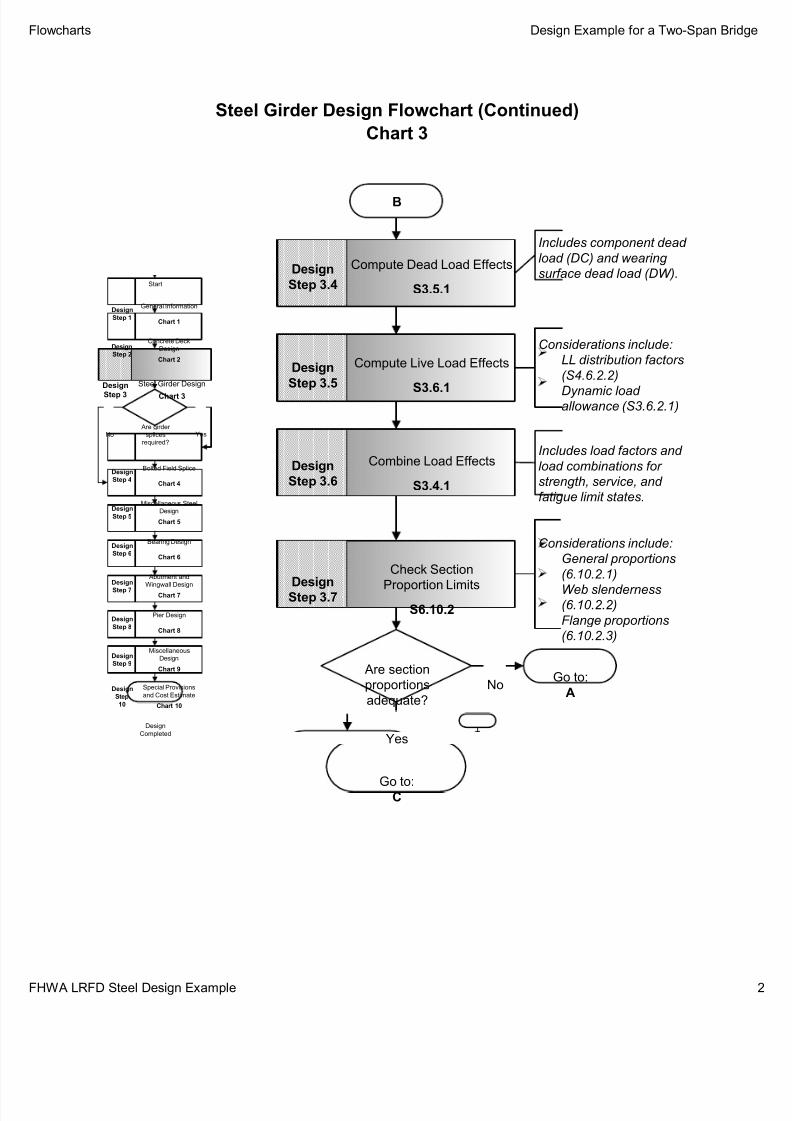
Steel Girder Design Flowchart (Continued)
B
Are girder
splices
required?
Bolted Field Splice
Chart 4
Design
Step 4
Steel Girder Design
Chart 3
Design
Step 3
Concrete Deck
Design
Chart 2
Design
Step 2
No Yes
Miscellaneous Steel
Design
Chart 5
Design
Step 5
Design
Completed
Bearing Design
Chart 6
Design
Step 6
Miscellaneous
Design
Chart 9
Design
Step 9
Abutment and
Wingwall Design
Chart 7
Design
Step 7
Pier Design
Chart 8
Design
Step 8
Special Provisions
and Cost Estimate
Chart 10
Design
Step
10
Start
General Information
Chart 1
Design
Step 1
Chart 3
Combine Load Effects
S3.4.1
Design
Step 3.6
Compute Dead Load Effects
S3.5.1
Design
Step 3.4
Compute Live Load Effects
S3.6.1
Design
Step 3.5
Includes component dead
load (DC) and wearing
surface dead load (DW).
Considerations include:
LL distribution factors
(S4.6.2.2)
Dynamic load allowance (S3.6.2.1)
Includes load factors and
load combinations for
strength, service, and
fatigue limit states.
Are section
proportions
adequate?
Check Section
Proportion LimitsS6.10.2
Design
Step 3.7
Yes
NoGo to:
A
Go to:C
Considerations include:
General proportions
(6.10.2.1)
Web slenderness(6.10.2.2)
Flange proportions
(6.10.2.3)
Flowcharts Design Example for a Two-Span Brid
FHWA LRFD Steel Design Example
7/29/2019 LRFD steel design.pdf
http://slidepdf.com/reader/full/lrfd-steel-designpdf 18/646
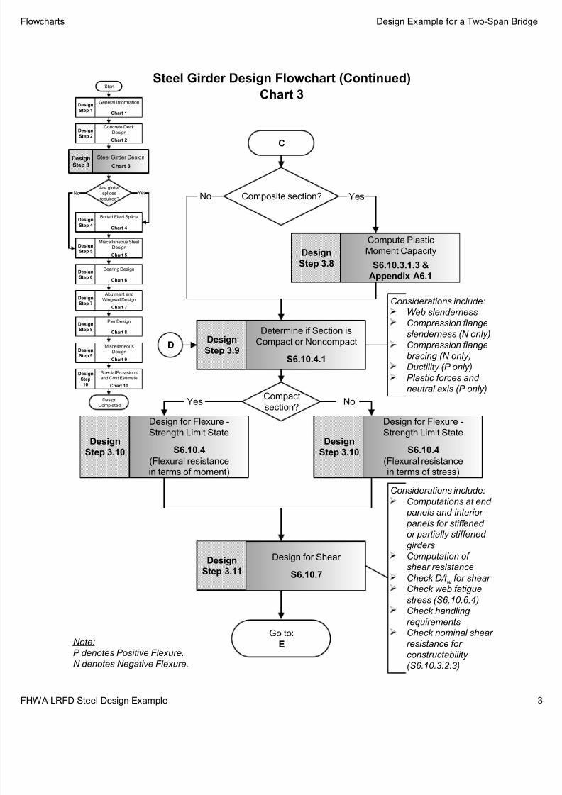
Steel Girder Design Flowchart (Continued)
Note:
P denotes Positive Flexure.
N denotes Negative Flexure.
C
Chart 3
Compute Plastic
Moment Capacity
S6.10.3.1.3 &
Appendix A6.1
Design
Step 3.8
Composite section? YesNo
Design for Flexure -
Strength Limit State
S6.10.4
(Flexural resistance
in terms of moment)
Design
Step 3.10
Determine if Section is
Compact or Noncompact
S6.10.4.1
Design
Step 3.9
Compact
section?
Design for Flexure -
Strength Limit State
S6.10.4
(Flexural resistance
in terms of stress)
Design
Step 3.10
NoYes
D
Considerations include:
Web slenderness
Compression flange
slenderness (N only)
Compression flange
bracing (N only)
Ductility (P only)
Plastic forces and
neutral axis (P only)
Go to:
E
Design for Shear
S6.10.7
DesignStep 3.11
Considerations include:
Computations at end
panels and interior
panels for stiffened
or partially stiffened
girders
Computation of shear resistance
Check D/t w
for shear
Check web fatigue
stress (S6.10.6.4)
Check handling
requirements
Check nominal shear
resistance for
constructability
(S6.10.3.2.3)
Are girder
splices
required?
Bolted Field Splice
Chart 4
Design
Step 4
Steel Girder Design
Chart 3
Design
Step 3
Concrete Deck
Design
Chart 2
Design
Step 2
No Yes
Miscellaneous Steel
Design
Chart 5
Design
Step 5
Design
Completed
Bearing Design
Chart 6
Design
Step 6
Miscellaneous
Design
Chart 9
Design
Step 9
Abutment and
Wingwall Design
Chart 7
Design
Step 7
Pier Design
Chart 8
Design
Step 8
Special Provisions
and Cost Estimate
Chart 10
Design
Step
10
Start
General Information
Chart 1
Design
Step 1
Flowcharts Design Example for a Two-Span Brid
FHWA LRFD Steel Design Example

7/29/2019 LRFD steel design.pdf
http://slidepdf.com/reader/full/lrfd-steel-designpdf 19/646
Steel Girder Design Flowchart (Continued)
E
Are girder splices
required?
Bolted Field Splice
Chart 4
Design
Step 4
Steel Girder Design
Chart 3
Design
Step 3
Concrete Deck
Design
Chart 2
Design
Step 2
No Yes
Miscellaneous Steel
Design
Chart 5
Design
Step 5
Design
Completed
Bearing Design
Chart 6
Design
Step 6
Miscellaneous
Design
Chart 9
Design
Step 9
Abutment and
Wingwall Design
Chart 7
Design
Step 7
Pier Design
Chart 8
Design
Step 8
Special Provisions
and Cost Estimate
Chart 10
Design
Step
10
Start
General Information
Chart 1
Design
Step 1
Go to:
F
Chart 3
Design Transverse
Intermediate Stiffeners
S6.10.8.1
Design
Step 3.12
If no stiffeners are used,
then the girder must be
designed for shear based
on the use of an
unstiffened web.
Transverse
intermediate
stiffeners?No
Yes
Design includes:
Select single-plate or
double-plate
Compute projecting width, moment of
inertia, and area
Check slenderness
requirements
(S6.10.8.1.2)
Check stiffness
requirements
(S6.10.8.1.3)
Check strength
requirements
(S6.10.8.1.4)
Design Longitudinal
Stiffeners
S6.10.8.3
Design
Step 3.13
Design includes:
Determine required
locations
Select stiffener sizes
Compute projecting width and moment of
inertia
Check slenderness
requirements
Check stiffness
requirements
If no longitudinal stiffenersare used, then the girder
must be designed for shear
based on the use of either
an unstiffened or a
transversely stiffened web,
as applicable.
Longitudinal
stiffeners?No
Yes
Flowcharts Design Example for a Two-Span Brid
FHWA LRFD Steel Design Example

7/29/2019 LRFD steel design.pdf
http://slidepdf.com/reader/full/lrfd-steel-designpdf 20/646
Steel Girder Design Flowchart (Continued)
F
Are girder splices
required?
Bolted Field Splice
Chart 4
Design
Step 4
Steel Girder Design
Chart 3
Design
Step 3
Concrete Deck
Design
Chart 2
Design
Step 2
No Yes
Miscellaneous Steel
Design
Chart 5
Design
Step 5
Design
Completed
Bearing Design
Chart 6
Design
Step 6
Miscellaneous
Design
Chart 9
Design
Step 9
Abutment and
Wingwall Design
Chart 7
Design
Step 7
Pier Design
Chart 8
Design
Step 8
Special Provisions
and Cost Estimate
Chart 10
Design
Step
10
Start
General Information
Chart 1
Design
Step 1
Chart 3
Design for Flexure -
Fatigue and Fracture
Limit State
S6.6.1.2 & S6.10.6
Design
Step 3.14
Check:
Fatigue load
(S3.6.1.4)
Load-induced fatigue
(S6.6.1.2)
Fatigue requirements
for webs (S6.10.6)
Distortion induced
fatigue
Fracture
Is stiffened web
most cost effective?YesNo
Use unstiffened
web in steel
girder design.
Use stiffened
web in steel
girder design.
Design for Flexure -
Constructibility Check
S6.10.3.2
DesignStep 3.16
Check:
Web slenderness
Compression flange
slenderness
Compression flange
bracing
Shear
Design for Flexure -
Service Limit State
S2.5.2.6.2 & S6.10.5
Design
Step 3.15
Compute:
Live load deflection
(optional)
(S2.5.2.6.2)
Permanent deflection
(S6.10.5)
Go to:
G
Flowcharts Design Example for a Two-Span Brid
FHWA LRFD Steel Design Example

7/29/2019 LRFD steel design.pdf
http://slidepdf.com/reader/full/lrfd-steel-designpdf 21/646
Return to
Main Flowchart
Steel Girder Design Flowchart (Continued)
G
Are girder
splices
required?
Bolted Field Splice
Chart 4
Design
Step 4
Steel Girder Design
Chart 3
Design
Step 3
Concrete Deck
Design
Chart 2
Design
Step 2
No Yes
Miscellaneous Steel
Design
Chart 5
Design
Step 5
Design
Completed
Bearing Design
Chart 6
Design
Step 6
Miscellaneous
Design
Chart 9
Design
Step 9
Abutment and
Wingwall Design
Chart 7
Design
Step 7
Pier Design
Chart 8
Design
Step 8
Special Provisions
and Cost Estimate
Chart 10
Design
Step
10
Start
General Information
Chart 1
Design
Step 1
Have all positive
and negative flexure
design sections been
checked?
Yes
No
Go to:
D (and repeat
flexural checks)
Check Wind Effects
on Girder Flanges
S6.10.3.5
Design
Step 3.17
Refer to Design Step 3.9
for determination of
compact or noncompact
section.
Chart 3
Draw Schematic of Final
Steel Girder Design
Design
Step 3.18
Were all specificationchecks satisfied, and is the
girder optimized?
Yes
NoGo to:
A
Flowcharts Design Example for a Two-Span Brid
FHWA LRFD Steel Design Example

7/29/2019 LRFD steel design.pdf
http://slidepdf.com/reader/full/lrfd-steel-designpdf 22/646
Bolted Field Splice Design Flowchart
Includes:
Splice location
Girder section
properties
Material and bolt
properties
Start
Are girder
splices
required?
Steel Girder Design
Chart 3
Design
Step 3
Bolted Field Splice
Design
Chart 4
Design
Step 4
Concrete Deck
Design
Chart 2
Design
Step 2
No Yes
Miscellaneous Steel
Design
Chart 5
Design
Step 5
Design
Completed
Bearing Design
Chart 6
Design
Step 6
Miscellaneous
Design
Chart 9
Design
Step 9
Abutment and
Wingwall Design
Chart 7
Design
Step 7
Pier Design
Chart 8
Design
Step 8
Special Provisions
and Cost Estimate
Chart 10
Design
Step
10
Start
General Information
Chart 1
Design
Step 1
Compute Flange Splice
Design Loads
6.13.6.1.4c
Design
Step 4.3
Design bolted field splice
based on the smaller
adjacent girder section
(S6.13.6.1.1).
Which adjacent
girder section is
smaller?
Design bolted field
splice based onright adjacent girder
section properties.
RightLeft
Design bolted field
splice based onleft adjacent girder
section properties.
Obtain Design CriteriaDesign
Step 4.1
Select Girder Section
as Basis for
Field Splice DesignS6.13.6.1.1
Design
Step 4.2
Go to:
A
Includes:
Girder moments
Strength stresses and
forces
Service stresses and
forces
Fatigue stresses and
forces
Controlling and non-controlling flange
Construction
moments and shears
Chart 4
Flowcharts Design Example for a Two-Span Brid
FHWA LRFD Steel Design Example
7/29/2019 LRFD steel design.pdf
http://slidepdf.com/reader/full/lrfd-steel-designpdf 23/646
A
Go to:
B
Bolted Field Splice Design Flowchart (Continued)
Are girder
splices
required?
Steel Girder Design
Chart 3
Design
Step 3
Bolted Field Splice
Design
Chart 4
Design
Step 4
Concrete Deck
Design
Chart 2
Design
Step 2
No Yes
Miscellaneous Steel
Design
Chart 5
Design
Step 5
Design
Completed
Bearing Design
Chart 6
Design
Step 6
Miscellaneous
Design
Chart 9
Design
Step 9
Abutment and
Wingwall Design
Chart 7
Design
Step 7
Pier Design
Chart 8
Design
Step 8
Special Provisions
and Cost Estimate
Chart 10
Design
Step
10
Start
General Information
Chart 1
Design
Step 1
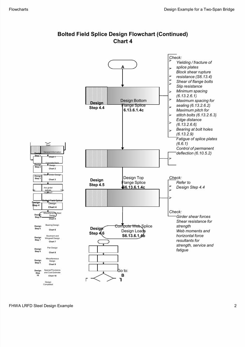
Design Bottom
Flange Splice
6.13.6.1.4c
Design
Step 4.4
Compute Web Splice
Design Loads
S6.13.6.1.4b
Design
Step 4.6
Check:
Girder shear forces
Shear resistance for
strength
Web moments and
horizontal force
resultants for
strength, service and
fatigue
Design Top
Flange SpliceS6.13.6.1.4c
Design
Step 4.5
Check:
Refer toDesign Step 4.4
Check:
Yielding / fracture of
splice plates
Block shear rupture
resistance (S6.13.4)
Shear of flange bolts
Slip resistance
Minimum spacing
(6.13.2.6.1)
Maximum spacing for
sealing (6.13.2.6.2)
Maximum pitch for
stitch bolts (6.13.2.6.3)
Edge distance(6.13.2.6.6)
Bearing at bolt holes
(6.13.2.9)
Fatigue of splice plates
(6.6.1)
Control of permanent
deflection (6.10.5.2)
Chart 4
Flowcharts Design Example for a Two-Span Brid
FHWA LRFD Steel Design Example

7/29/2019 LRFD steel design.pdf
http://slidepdf.com/reader/full/lrfd-steel-designpdf 24/646
Bolted Field Splice Design Flowchart (Continued)
Are girder
splices
required?
Steel Girder Design
Chart 3
Design
Step 3
Bolted Field Splice
Design
Chart 4
Design
Step 4
Concrete Deck
Design
Chart 2
Design
Step 2
No Yes
Miscellaneous Steel
Design
Chart 5
Design
Step 5
Design
Completed
Bearing Design
Chart 6
Design
Step 6
Miscellaneous
Design
Chart 9
Design
Step 9
Abutment and
Wingwall Design
Chart 7
Design
Step 7
Pier Design
Chart 8
Design
Step 8
Special Provisions
and Cost Estimate
Chart 10
Design
Step
10
Start
General Information
Chart 1
Design
Step 1
Both the top and bottom
flange splices must be
designed, and they are
designed using the same
procedures.
Are both the top and
bottom flange splice
designs completed?
No
Yes
Go to:
A
Do all bolt
patterns satisfy all
specifications?
Yes
NoGo to:
A
Chart 4
Return to
Main Flowchart
Draw Schematic of Final
Bolted Field Splice Design
Design
Step 4.8
Design Web Splice
S6.13.6.1.4b
Design
Step 4.7
Check:
Bolt shear strength
Shear yielding of splice plate
(6.13.5.3)
Fracture on the net
section (6.13.4)
Block shear rupture
resistance (6.13.4)
Flexural yielding of
splice plates
Bearing resistance
(6.13.2.9)
Fatigue of splice
plates (6.6.1.2.2)
B
Flowcharts Design Example for a Two-Span Brid
FHWA LRFD Steel Design Example
7/29/2019 LRFD steel design.pdf
http://slidepdf.com/reader/full/lrfd-steel-designpdf 25/646
Miscellaneous Steel Design Flowchart
Start
Go to:
A
Concrete Deck
Design
Chart 2
DesignStep 2
Design
Completed
Bearing Design
Chart 6
DesignStep 6
Miscellaneous
Design
Chart 9
Design
Step 9
Abutment and
Wingwall Design
Chart 7
Design
Step 7
Pier Design
Chart 8
Design
Step 8
Special Provisions
and Cost Estimate
Chart 10
Design
Step
10
Start
General Information
Chart 1
Design
Step 1
Steel Girder Design
Chart 3
Design
Step 3
Miscellaneous Steel
Design
Chart 5
Design
Step 5
Are girder
splices
required?
Bolted Field Splice
Chart 4
Design
Step 4
No Yes
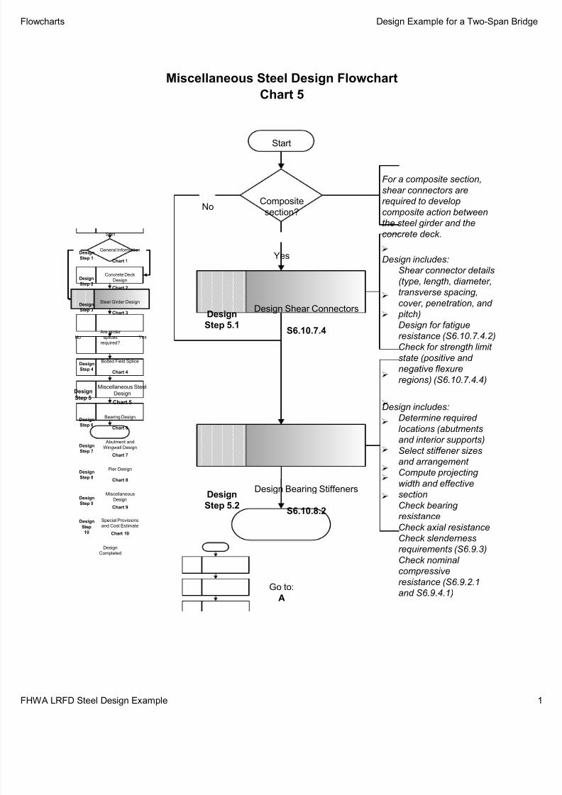
For a composite section,
shear connectors are
required to develop
composite action between
the steel girder and the
concrete deck.
Composite
section?No
Yes
Design Shear Connectors
S6.10.7.4
Design
Step 5.1
Design includes:
Shear connector details
(type, length, diameter,transverse spacing,
cover, penetration, and
pitch)
Design for fatigue
resistance (S6.10.7.4.2)
Check for strength limit
state (positive and
negative flexure
regions) (S6.10.7.4.4)
Chart 5
Design Bearing Stiffeners
S6.10.8.2
Design
Step 5.2
Design includes:
Determine required locations (abutments
and interior supports)
Select stiffener sizes
and arrangement
Compute projecting
width and effective
section
Check bearing
resistance
Check axial resistance
Check slenderness
requirements (S6.9.3)
Check nominal compressive
resistance (S6.9.2.1
and S6.9.4.1)
Flowcharts Design Example for a Two-Span Brid
FHWA LRFD Steel Design Example
7/29/2019 LRFD steel design.pdf
http://slidepdf.com/reader/full/lrfd-steel-designpdf 26/646
Miscellaneous Steel Design Flowchart (Continued)
Go to:
B
Concrete Deck
Design
Chart 2
Design
Step 2
Design
Completed
Bearing Design
Chart 6
Design
Step 6
Miscellaneous
Design
Chart 9
Design
Step 9
Abutment and
Wingwall Design
Chart 7
Design
Step 7
Pier Design
Chart 8
Design
Step 8
Special Provisions
and Cost Estimate
Chart 10
Design
Step
10
Start
General Information
Chart 1
Design
Step 1
Steel Girder Design
Chart 3
Design
Step 3
Miscellaneous Steel
Design
Chart 5
Design
Step 5
Are girder
splices
required?
Bolted Field Splice
Chart 4
Design
Step 4
No Yes
A
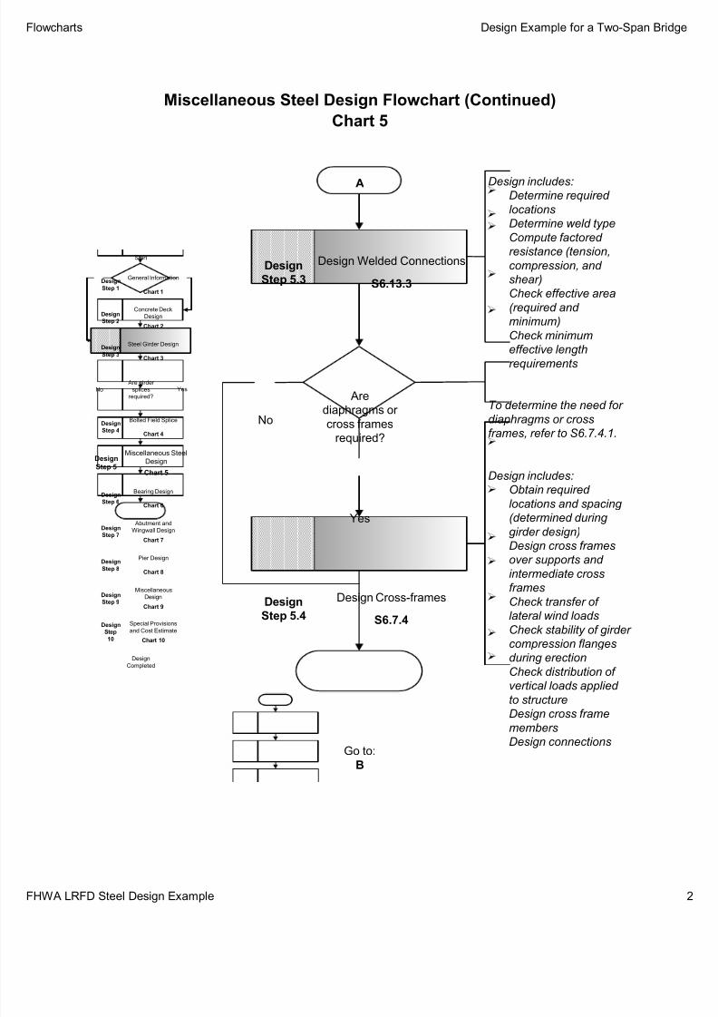
Design Welded Connections
S6.13.3
Design
Step 5.3
Design includes:Determine required
locations
Determine weld type
Compute factored
resistance (tension,
compression, and
shear)
Check effective area
(required and
minimum)
Check minimum
effective length
requirements
Chart 5
To determine the need for
diaphragms or cross
frames, refer to S6.7.4.1.
Are
diaphragms or
cross frames
required?
No
Yes
Design Cross-frames
S6.7.4
Design
Step 5.4
Design includes:
Obtain required
locations and spacing
(determined during
girder design)Design cross frames
over supports and
intermediate cross
frames
Check transfer of
lateral wind loads
Check stability of girder
compression flanges
during erection
Check distribution of
vertical loads applied
to structure
Design cross framemembers
Design connections
Flowcharts Design Example for a Two-Span Brid
FHWA LRFD Steel Design Example

7/29/2019 LRFD steel design.pdf
http://slidepdf.com/reader/full/lrfd-steel-designpdf 27/646
Miscellaneous Steel Design Flowchart (Continued)
Concrete Deck
Design
Chart 2
Design
Step 2
Design
Completed
Bearing Design
Chart 6
Design
Step 6
Miscellaneous
Design
Chart 9
Design
Step 9
Abutment and
Wingwall Design
Chart 7
Design
Step 7
Pier Design
Chart 8
Design
Step 8
Special Provisions
and Cost Estimate
Chart 10
Design
Step
10
Start
General Information
Chart 1
Design
Step 1
Steel Girder Design
Chart 3
Design
Step 3
Miscellaneous Steel
Design
Chart 5
Design
Step 5
Are girder
splices
required?
Bolted Field Splice
Chart 4
Design
Step 4
No Yes
B
To determine the need for
lateral bracing, refer to
S6.7.5.1.
Is lateral
bracing
required?No
Yes
Design Lateral Bracing
S6.7.5
Design
Step 5.5
Design includes:
Check transfer of lateral wind loads
Check control of
deformation during
erection and placement
of deck
Design bracing
members
Design connections
Chart 5
Compute Girder Camber
S6.7.2
Design
Step 5.6
Compute the following
camber components:
Camber due to dead
load of structural steel
Camber due to dead
load of concrete deck
Camber due to
superimposed dead
load
Camber due to vertical
profile
Residual camber (if
any)
Total camber Return to
Main Flowchart
Flowcharts Design Example for a Two-Span Brid
FHWA LRFD Steel Design Example

7/29/2019 LRFD steel design.pdf
http://slidepdf.com/reader/full/lrfd-steel-designpdf 28/646
Bearing Design Flowchart
Start
Go to:
B
Select OptimumBearing Type
S14.6.2
Design
Step 6.2
Concrete Deck
Design
Chart 2
Design
Step 2
Design
Completed
Miscellaneous
Design
Chart 9
Design
Step 9
Abutment and
Wingwall Design
Chart 7
Design
Step 7
Pier Design
Chart 8
Design
Step 8
Special Provisions
and Cost Estimate
Chart 10
Design
Step
10
Start
General Information
Chart 1
Design
Step 1
Steel Girder Design
Chart 3
Design
Step 3
Are girder
splices
required?
Bolted Field Splice
Chart 4
Design
Step 4
No Yes
Bearing Design
Chart 6
Design
Step 6
Miscellaneous Steel
Design
Chart 5
Design
Step 5
See list of bearing typesand selection criteria in
AASHTO Table 14.6.2-1.
Obtain Design CriteriaDesign
Step 6.1
Yes
Steel-
reinforced
elastomeric
bearing?
Design selected
bearing type
in accordance
with S14.7.
No
Includes:
Movement (longitudinal
and transverse)
Rotation (longitudinal,
transverse, and
vertical)
Loads (longitudinal,
transverse, and
vertical)
Includes:Pad length
Pad width
Thickness of
elastomeric layers
Number of steel
reinforcement layers
Thickness of steel
reinforcement layers
Edge distance
Material properties
ASelect Preliminary
Bearing Properties
Design
Step 6.3
Select Design Method
(A or B)
S14.7.5 or S14.7.6
Design
Step 6.4
Method A usually results ina bearing with a lower
capacity than Method B.
However, Method B
requires additional testing
and quality control
(SC14.7.5.1).
Note:
Method A is described in S14.7.6.
Method B is described in S14.7.5.
Chart 6
Flowcharts Design Example for a Two-Span Brid
FHWA LRFD Steel Design Example
7/29/2019 LRFD steel design.pdf
http://slidepdf.com/reader/full/lrfd-steel-designpdf 29/646
Bearing Design Flowchart (Continued)
Go to:
C
Concrete Deck
Design
Chart 2
Design
Step 2
Design
Completed
Miscellaneous
Design
Chart 9
Design
Step 9
Abutment and
Wingwall Design
Chart 7
Design
Step 7
Pier Design
Chart 8
Design
Step 8
Special Provisions
and Cost Estimate
Chart 10
Design
Step
10
Start
General Information
Chart 1
Design
Step 1
Steel Girder Design
Chart 3
Design
Step 3
Are girder
splices
required?
Bolted Field Splice
Chart 4
Design
Step 4
No Yes
Bearing Design
Chart 6
Design
Step 6
Miscellaneous Steel
Design
Chart 5
Design
Step 5
B
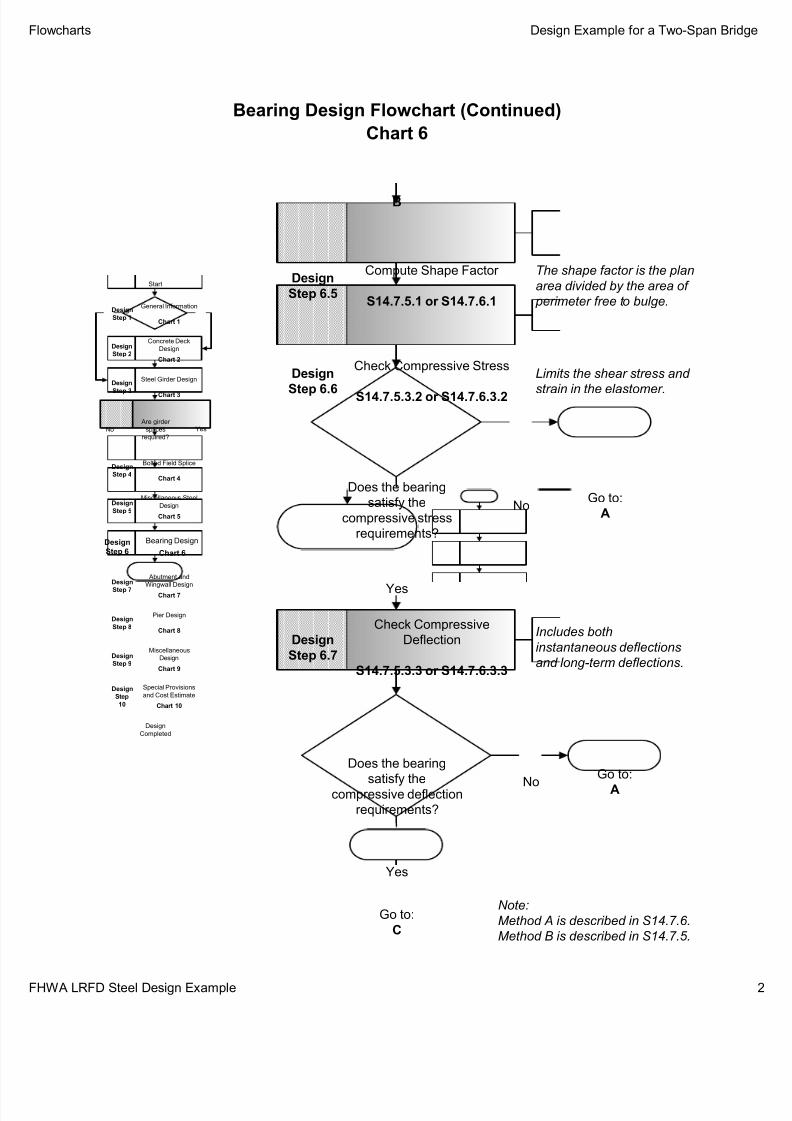
Compute Shape Factor
S14.7.5.1 or S14.7.6.1
Design
Step 6.5
The shape factor is the plan
area divided by the area of
perimeter free to bulge.
Check Compressive Stress
S14.7.5.3.2 or S14.7.6.3.2
Design
Step 6.6
Does the bearing
satisfy the
compressive stress
requirements?
NoGo to:
A
Yes
Limits the shear stress and
strain in the elastomer.
Check Compressive
Deflection
S14.7.5.3.3 or S14.7.6.3.3
Design
Step 6.7
Does the bearing
satisfy the
compressive deflection
requirements?
No
Go to:
A
Yes
Includes both
instantaneous deflections
and long-term deflections.
Note:
Method A is described in S14.7.6.
Method B is described in S14.7.5.
Chart 6
Flowcharts Design Example for a Two-Span Brid
FHWA LRFD Steel Design Example
7/29/2019 LRFD steel design.pdf
http://slidepdf.com/reader/full/lrfd-steel-designpdf 30/646
Bearing Design Flowchart (Continued)
Go to:
D
Concrete Deck
Design
Chart 2
Design
Step 2
Design
Completed
Miscellaneous
Design
Chart 9
Design
Step 9
Abutment and
Wingwall Design
Chart 7
Design
Step 7
Pier Design
Chart 8
Design
Step 8
Special Provisions
and Cost Estimate
Chart 10
Design
Step
10
Start
General Information
Chart 1
Design
Step 1
Steel Girder Design
Chart 3
Design
Step 3
Are girder
splices
required?
Bolted Field Splice
Chart 4
Design
Step 4
No Yes
Bearing Design
Chart 6
Design
Step 6
Miscellaneous Steel
Design
Chart 5
Design
Step 5
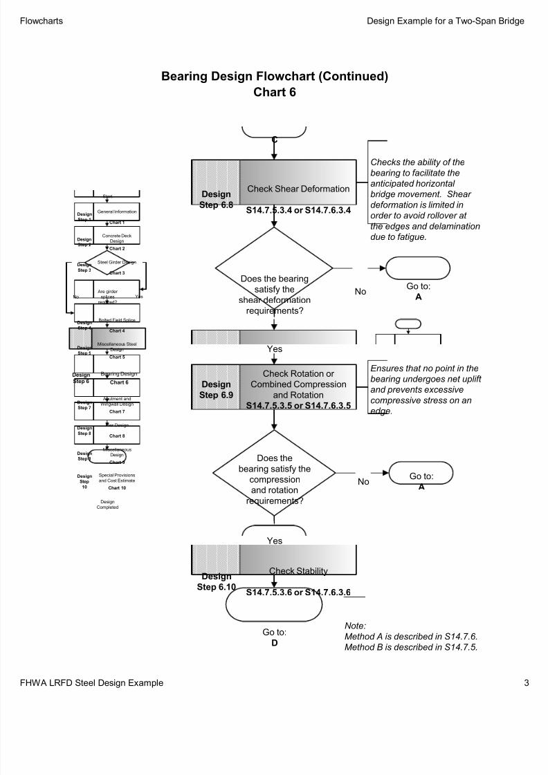
C
Does the bearing
satisfy the
shear deformation
requirements?
NoGo to:
A
Yes
Check Shear Deformation
S14.7.5.3.4 or S14.7.6.3.4
Design
Step 6.8
Checks the ability of the
bearing to facilitate the
anticipated horizontal
bridge movement. Shear
deformation is limited in
order to avoid rollover at
the edges and delamination
due to fatigue.
Check Rotation or
Combined Compression
and Rotation
S14.7.5.3.5 or S14.7.6.3.5
Design
Step 6.9
Ensures that no point in the
bearing undergoes net uplift
and prevents excessive
compressive stress on an
edge.
Does the
bearing satisfy the
compression
and rotation
requirements?
NoGo to:
A
Yes
Check Stability
S14.7.5.3.6 or S14.7.6.3.6
Design
Step 6.10
Note:
Method A is described in S14.7.6.
Method B is described in S14.7.5.
Chart 6
Flowcharts Design Example for a Two-Span Brid
FHWA LRFD Steel Design Example

7/29/2019 LRFD steel design.pdf
http://slidepdf.com/reader/full/lrfd-steel-designpdf 31/646
Bearing Design Flowchart (Continued)
Concrete Deck
Design
Chart 2
Design
Step 2
Design
Completed
Miscellaneous
Design
Chart 9
Design
Step 9
Abutment and
Wingwall Design
Chart 7
Design
Step 7
Pier Design
Chart 8
Design
Step 8
Special Provisions
and Cost Estimate
Chart 10
Design
Step
10
Start
General Information
Chart 1
Design
Step 1
Steel Girder Design
Chart 3
Design
Step 3
Are girder
splices
required?
Bolted Field Splice
Chart 4
Design
Step 4
No Yes
Bearing Design
Chart 6
Design
Step 6
Miscellaneous Steel
Design
Chart 5
Design
Step 5
D
Does the bearing
satisfy the
stability
requirements?
NoGo to:
A
Yes
Does the bearing
satisfy the
reinforcementrequirements?
NoGo to:
A
Yes
Check Reinforcement
S14.7.5.3.7 or S14.7.6.3.7
Design
Step 6.11
Checks that the
reinforcement can sustain
the tensile stresses induced
by compression in the
bearing.
Method A or
Method B?
Design for
Seismic Provisions
S14.7.5.3.8
Design
Step 6.12
Method B
Design for Anchorage
S14.7.6.4
Design
Step 6.12
Method A
Note:
Method A is described in S14.7.6.
Method B is described in S14.7.5.
Chart 6
Go to:
E
Flowcharts Design Example for a Two-Span Brid
FHWA LRFD Steel Design Example

7/29/2019 LRFD steel design.pdf
http://slidepdf.com/reader/full/lrfd-steel-designpdf 32/646
Bearing Design Flowchart (Continued)
Concrete Deck
Design
Chart 2
Design
Step 2
Design
Completed
Miscellaneous
Design
Chart 9
Design
Step 9
Abutment and
Wingwall Design
Chart 7
Design
Step 7
Pier Design
Chart 8
Design
Step 8
Special Provisions
and Cost Estimate
Chart 10
Design
Step
10
Start
General Information
Chart 1
Design
Step 1
Steel Girder Design
Chart 3
Design
Step 3
Are girder
splices
required?
Bolted Field Splice
Chart 4
Design
Step 4
No Yes
Bearing Design
Chart 6
Design
Step 6
Miscellaneous Steel
Design
Chart 5
Design
Step 5
E
Is the
bearing
fixed?
No
Yes
Design Anchoragefor Fixed Bearings
S14.8.3
Design
Step 6.13
Return to
Main Flowchart
Chart 6
Draw Schematic of
Final Bearing Design
Design
Step 6.14
Flowcharts Design Example for a Two-Span Brid
FHWA LRFD Steel Design Example
7/29/2019 LRFD steel design.pdf
http://slidepdf.com/reader/full/lrfd-steel-designpdf 33/646
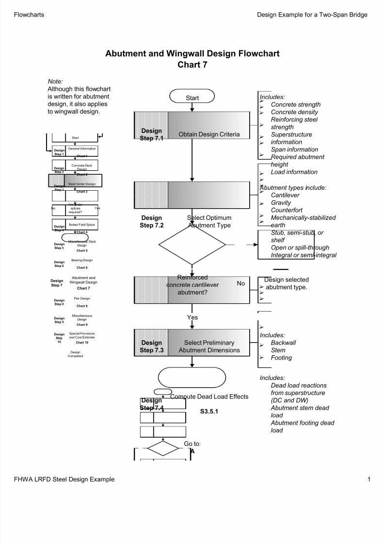
Abutment and Wingwall Design Flowchart
Start
Go to:
A
Select Optimum
Abutment Type
Design
Step 7.2
Abutment types include:Cantilever
Gravity
Counterfort
Mechanically-stabilized
earth
Stub, semi-stub, or
shelf
Open or spill-through
Integral or semi-integral
Obtain Design CriteriaDesign
Step 7.1
Yes
Reinforced
concrete cantilever abutment?
Design selected
abutment type.No
Includes:Concrete strength
Concrete density
Reinforcing steel
strength
Superstructure
information
Span information
Required abutment
height
Load information
Includes:
Dead load reactions
from superstructure
(DC and DW)
Abutment stem dead
load
Abutment footing dead
load
Compute Dead Load Effects
S3.5.1
Design
Step 7.4
Concrete Deck
Design
Chart 2
Design
Step 2
Design
Completed
Miscellaneous
Design
Chart 9
Design
Step 9
Special Provisions
and Cost Estimate
Chart 10
Design
Step
10
Start
General Information
Chart 1
Design
Step 1
Steel Girder Design
Chart 3
Design
Step 3
Are girder
splices
required?
Bolted Field Splice
Chart 4
Design
Step 4
No Yes
Abutment and
Wingwall Design
Chart 7
Design
Step 7
Miscellaneous Steel
Design
Chart 5
Design
Step 5
Bearing Design
Chart 6
Design
Step 6
Pier Design
Chart 8
Design
Step 8
Chart 7
Includes:
Backwall
Stem
Footing
Select Preliminary
Abutment Dimensions
Design
Step 7.3
Note:
Although this flowchart
is written for abutmentdesign, it also applies
to wingwall design.
Flowcharts Design Example for a Two-Span Brid
FHWA LRFD Steel Design Example
7/29/2019 LRFD steel design.pdf
http://slidepdf.com/reader/full/lrfd-steel-designpdf 34/646
Abutment and Wingwall Design Flowchart (Continued)
Go to:
B
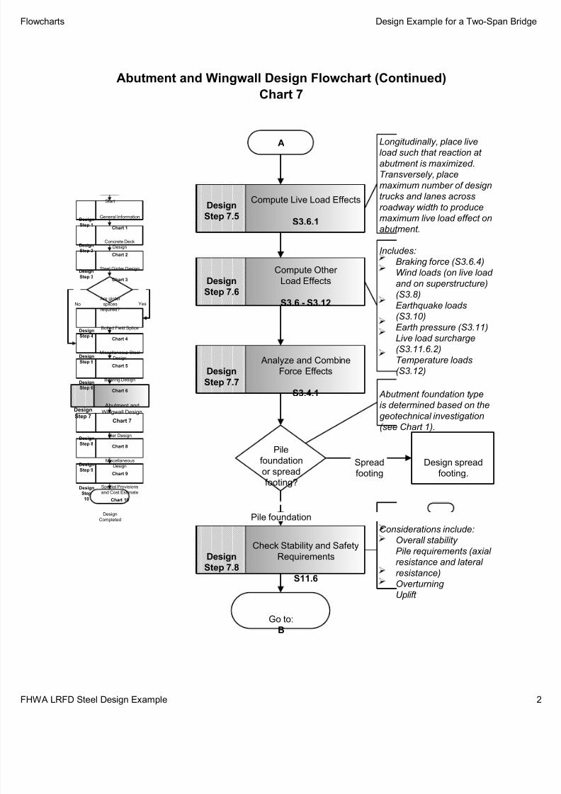
Analyze and Combine
Force Effects
S3.4.1
Design
Step 7.7
Compute Other
Load Effects
S3.6 - S3.12
DesignStep 7.6
Includes:
Braking force (S3.6.4)
Wind loads (on live load
and on superstructure)
(S3.8)
Earthquake loads
(S3.10)
Earth pressure (S3.11)
Live load surcharge
(S3.11.6.2)
Temperature loads
(S3.12)
Check Stability and Safety
Requirements
S11.6
DesignStep 7.8
Considerations include:
Overall stability
Pile requirements (axial
resistance and lateral
resistance)
Overturning
Uplift
A
Pile
foundation
or spread
footing?
Design spread
footing.
Spread
footing
Pile foundation
Abutment foundation type
is determined based on the
geotechnical investigation(see Chart 1).
Concrete Deck
Design
Chart 2
Design
Step 2
Design
Completed
Miscellaneous
Design
Chart 9
Design
Step 9
Special Provisions
and Cost Estimate
Chart 10
Design
Step
10
Start
General Information
Chart 1
Design
Step 1
Steel Girder Design
Chart 3
Design
Step 3
Are girder
splices
required?
Bolted Field Splice
Chart 4
Design
Step 4
No Yes
Abutment and
Wingwall Design
Chart 7
Design
Step 7
Miscellaneous Steel
Design
Chart 5
Design
Step 5
Bearing Design
Chart 6
Design
Step 6
Pier Design
Chart 8
Design
Step 8
Compute Live Load Effects
S3.6.1
Design
Step 7.5
Longitudinally, place liveload such that reaction at
abutment is maximized.
Transversely, place
maximum number of design
trucks and lanes across
roadway width to produce
maximum live load effect on
abutment.
Chart 7
Flowcharts Design Example for a Two-Span Brid
FHWA LRFD Steel Design Example

7/29/2019 LRFD steel design.pdf
http://slidepdf.com/reader/full/lrfd-steel-designpdf 35/646
Abutment and Wingwall Design Flowchart (Continued)
B
No
Return to
Main Flowchart
Design Abutment Footing
Section 5
Design
Step 7.11
Concrete Deck
Design
Chart 2
Design
Step 2
Design
Completed
Miscellaneous
Design
Chart 9
Design
Step 9
Special Provisions
and Cost Estimate
Chart 10
Design
Step
10
Start
General Information
Chart 1
Design
Step 1
Steel Girder Design
Chart 3
Design
Step 3
Are girder
splices
required?
Bolted Field Splice
Chart 4
Design
Step 4
No Yes
Abutment and
Wingwall Design
Chart 7
Design
Step 7
Miscellaneous Steel
Design
Chart 5
Design
Step 5
Bearing Design
Chart 6
Design
Step 6
Pier Design
Chart 8
Design
Step 8
Design Abutment Stem
Section 5
Design
Step 7.10
Design Abutment Backwall
Section 5
Design
Step 7.9
Design includes:
Design for flexure
Design for shear
Check crack control
Chart 7
Draw Schematic of
Final Abutment Design
Design
Step 7.12
Is a pile
foundation being
used?
Yes
Go to:
Design Step P
Design includes:
Design for flexure
Design for shear
Check crack control
Design includes:
Design for flexure
Design for shear
Check crack control
Flowcharts Design Example for a Two-Span Brid
FHWA LRFD Steel Design Example

7/29/2019 LRFD steel design.pdf
http://slidepdf.com/reader/full/lrfd-steel-designpdf 36/646
Pier Design Flowchart
Start
Go to:
A
Select Optimum
Pier Type
Design
Step 8.2
Concrete Deck
Design
Chart 2
Design
Step 2
Design
Completed
Miscellaneous
Design
Chart 9
Design
Step 9
Abutment and
Wingwall Design
Chart 7
Design
Step 7
Special Provisions
and Cost Estimate
Chart 10
Design
Step
10
Start
General Information
Chart 1
Design
Step 1
Steel Girder Design
Chart 3
Design
Step 3
Are girder
splices
required?
Bolted Field Splice
Chart 4
Design
Step 4
No Yes
Pier Design
Chart 8
Design
Step 8
Miscellaneous Steel
Design
Chart 5
Design
Step 5
Pier types include:
Hammerhead
Multi-column
Wall type
Pile bent
Single column
Obtain Design CriteriaDesign
Step 8.1
Yes
Reinforced
concrete
hammerhead
pier?
Design selected
pier type.No
Includes:
Concrete strength
Concrete density
Reinforcing steel
strength
Superstructure
information
Span information
Required pier height
Includes:
Dead load reactions
from superstructure(DC and DW)
Pier cap dead load
Pier column dead load
Pier footing dead load
Compute Dead Load Effects
S3.5.1
DesignStep 8.4
Bearing Design
Chart 6
Design
Step 6
Chart 8
Includes:
Pier cap
Pier column
Pier footing
Select Preliminary
Pier Dimensions
Design
Step 8.3
Flowcharts Design Example for a Two-Span Brid
FHWA LRFD Steel Design Example

7/29/2019 LRFD steel design.pdf
http://slidepdf.com/reader/full/lrfd-steel-designpdf 37/646
Pier Design Flowchart (Continued)
Go to:
B
Analyze and Combine
Force Effects
S3.4.1
DesignStep 8.7
Concrete Deck
Design
Chart 2
Design
Step 2
Design
Completed
Miscellaneous
Design
Chart 9
Design
Step 9
Abutment and
Wingwall Design
Chart 7
Design
Step 7
Special Provisions
and Cost Estimate
Chart 10
Design
Step
10
Start
General Information
Chart 1
Design
Step 1
Steel Girder Design
Chart 3
Design
Step 3
Are girder
splices
required?
Bolted Field Splice
Chart 4
Design
Step 4
No Yes
Pier Design
Chart 8
Design
Step 8
Miscellaneous Steel
Design
Chart 5
Design
Step 5
Compute Other
Load Effects
S3.6 - S3.14
Design
Step 8.6
Includes:
Centrifugal forces
(S3.6.3)Braking force (S3.6.4)
Vehicular collision force
(S3.6.5)
Water loads (S3.7)
Wind loads (on live
load, on superstructure,
and on pier) (S3.8)
Ice loads (S3.9)
Earthquake loads
(S3.10)
Earth pressure (S3.11)
Temperature loads
(S3.12)Vessel collision (S3.14)
Design includes:
Design for flexure
(negative)
Design for shear and
torsion (stirrups and
longitudinal torsion
reinforcement)
Check crack control
Design Pier Cap
Section 5
Design
Step 8.8
Design Pier Column
Section 5
Design
Step 8.9
Design includes:
Slenderness
considerations
Interaction of axial and
moment resistance
Design for shear
Bearing Design
Chart 6
Design
Step 6
A
Compute Live Load Effects
S3.6.1
Design
Step 8.5
Longitudinally, place liveload such that reaction at
pier is maximized.
Transversely, place design
trucks and lanes across
roadway width at various
locations to provide various
different loading conditions.
Pier design must satisfy all
live load cases.
Chart 8
Flowcharts Design Example for a Two-Span Brid
FHWA LRFD Steel Design Example

7/29/2019 LRFD steel design.pdf
http://slidepdf.com/reader/full/lrfd-steel-designpdf 38/646
Pier Design Flowchart (Continued)
Concrete Deck
Design
Chart 2
Design
Step 2
Design
Completed
Miscellaneous
Design
Chart 9
Design
Step 9
Abutment and
Wingwall Design
Chart 7
Design
Step 7
Special Provisions
and Cost Estimate
Chart 10
Design
Step
10
Start
General Information
Chart 1
Design
Step 1
Steel Girder Design
Chart 3
Design
Step 3
Are girder
splices
required?
Bolted Field Splice
Chart 4
Design
Step 4
No Yes
Pier Design
Chart 8
Design
Step 8
Miscellaneous Steel
Design
Chart 5
Design
Step 5
Bearing Design
Chart 6
Design
Step 6
B
Return to
Main Flowchart
Design Pier Footing
Section 5
Design
Step 8.11
Design includes:
Design for flexure
Design for shear (one-
way and two-way)
Crack control
Chart 8
Draw Schematic of
Final Pier Design
Design
Step 8.12
No
Is a pile
foundation being
used?
Yes
Go to:
Design Step P
Design Pier Piles
S10.7
Design
Step 8.10
Flowcharts Design Example for a Two-Span Brid
FHWA LRFD Steel Design Example
7/29/2019 LRFD steel design.pdf
http://slidepdf.com/reader/full/lrfd-steel-designpdf 39/646
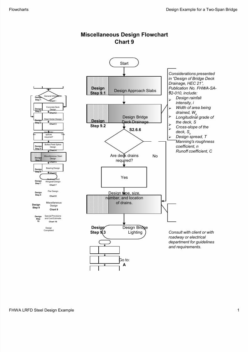
Miscellaneous Design Flowchart
Start
Design Approach SlabsDesign
Step 9.1
Are deck drains
required?No
Design Bridge
Deck DrainageS2.6.6
Design
Step 9.2
Design type, size,
number, and location
of drains.
Yes
Design Bridge
Lighting
Design
Step 9.3
Design
Completed
Start
Miscellaneous
Design
Chart 9
Design
Step 9
General Information
Chart 1
Design
Step 1
Are girder
splices
required?
Bolted Field Splice
Design
Chart 4
Design
Step 4
Steel Girder Design
Chart 3
Design
Step 3
No Yes
Miscellaneous Steel
Design
Chart 5
Design
Step 5
Bearing Design
Chart 6
Design
Step 6
Abutment and
Wingwall Design
Chart 7
Design
Step 7
Pier Design
Chart 8
Design
Step 8
Concrete Deck
Design
Chart 2
Design
Step 2
Special Provisions
and Cost Estimate
Chart 10
Design
Step
10
Considerations presented
in “Design of Bridge Deck
Drainage, HEC 21”,
Publication No. FHWA-SA-
92-010, include:
Design rainfall
intensity, i
Width of area being
drained, W p
Longitudinal grade of
the deck, SCross-slope of the
deck, S x
Design spread, T
Manning's roughness
coefficient, n
Runoff coefficient, C
Consult with client or with
roadway or electrical
department for guidelines
and requirements.
Chart 9
Go to:
A
Flowcharts Design Example for a Two-Span Brid
FHWA LRFD Steel Design Example

7/29/2019 LRFD steel design.pdf
http://slidepdf.com/reader/full/lrfd-steel-designpdf 40/646
Miscellaneous Design Flowchart (Continued)
Check for Bridge
Constructibility
S2.5.3
Design
Step 9.4
Design
Completed
Start
Miscellaneous
Design
Chart 9
Design
Step 9
General Information
Chart 1
Design
Step 1
Are girder
splices
required?
Bolted Field Splice
Design
Chart 4
Design
Step 4
Steel Girder Design
Chart 3
Design
Step 3
No Yes
Miscellaneous Steel
Design
Chart 5
Design
Step 5
Bearing Design
Chart 6
Design
Step 6
Abutment and
Wingwall Design
Chart 7
Design
Step 7
Pier Design
Chart 8
Design
Step 8
Concrete Deck
Design
Chart 2
Design
Step 2
Special Provisions
and Cost Estimate
Chart 10
Design
Step
10
A
Design type, size,
number, and location
of bridge lights.
Complete Additional Design
Considerations
Design
Step 9.5
Are there any
additional design
considerations?
Yes
No
Return to
Main Flowchart
The bridge should be
designed such that
fabrication and erection
can be completed
without undue difficulty
and such that locked-in
construction force
effects are withintolerable limits.
Is bridge lightingrequired?
Yes
No
Chart 9
Flowcharts Design Example for a Two-Span Brid
FHWA LRFD Steel Design Example

7/29/2019 LRFD steel design.pdf
http://slidepdf.com/reader/full/lrfd-steel-designpdf 41/646
Special Provisions and Cost Estimate Flowchart
Includes:
Develop list of required
special provisions
Obtain standard
special provisions from
client
Develop remaining
special provisions
Start
Develop Special ProvisionsDesign
Step 10.1
Return to
Main Flowchart
Does the
client have any
standard special
provisions?
Includes:
Obtain list of item
numbers and item
descriptions from client
Develop list of project
items
Compute estimated
quantities
Determine estimated
unit prices
Determine contingency
percentage
Compute estimated
total construction cost
Compute Estimated
Construction Cost
Design
Step 10.2
Design
Completed
Start
Special Provisions
and Cost Estimate
Chart 10
Design
Step 10
General Information
Chart 1
Design
Step 1
Are girder
splices
required?
Bolted Field Splice
Design
Chart 4
Design
Step 4
Steel Girder Design
Chart 3
DesignStep 3
No Yes
Miscellaneous Steel
Design
Chart 5
Design
Step 5
Bearing Design
Chart 6
Design
Step 6
Miscellaneous
Design
Chart 9
Design
Step 9
Abutment and
Wingwall Design
Chart 7
DesignStep 7
Pier Design
Chart 8
Design
Step 8
Concrete Deck
Design
Chart 2
Design
Step 2
Yes
Use and adapt
the client’s standard
special provisions as
applicable.
No
Develop new
special provisions as
needed.
Chart 10
Flowcharts Design Example for a Two-Span Brid
FHWA LRFD Steel Design Example

7/29/2019 LRFD steel design.pdf
http://slidepdf.com/reader/full/lrfd-steel-designpdf 42/646
Pile Foundation Design Flowchart
Start
Go to:
B
Determine Applicable Loads
and Load Combinations
S3
DesignStep P.2
Loads and load
combinations aredetermined in previous
design steps.
Chart P
Define Subsurface
Conditions and Any
Geometric Constraints
S10.4
Design
Step P.1
Subsurface exploration and
geotechnical
recommendations are
usually separate tasks.
Factor Loads for
Each Combination
S3
Design
Step P.3
Loads and load
combinations are
determined in previous
design steps.
Verify Need for a
Pile Foundation
S10.6.2.2
Design
Step P.4
Refer to FHWA-HI-96-033,
Section 7.3.
Select Suitable Pile Type
and Size Based on
Factored Loads and
Subsurface Conditions
Design
Step P.5
Guidance on pile type
selection is provided in
FHWA-HI-96-033, Chapter
8.
A
Concrete Deck
Design
Chart 2
Design
Step 2
Design
Completed
Bearing Design
Chart 6
Design
Step 6
Miscellaneous
Design
Chart 9
Design
Step 9
Abutment and
Wingwall Design
Chart 7
Design
Step 7
Pier Design
Chart 8
Design
Step 8
Special Provisions
and Cost Estimate
Chart 10
Design
Step
10
Start
General Information
Chart 1
Design
Step 1
Steel Girder Design
Chart 3
Design
Step 3
Are girder
splices
required?
Bolted Field
Splice Design
Chart 4
Design
Step 4
No Yes
Miscellaneous Steel
Design
Chart 5
Design
Step 5
Flowcharts Design Example for a Two-Span Brid
FHWA LRFD Steel Design Example

7/29/2019 LRFD steel design.pdf
http://slidepdf.com/reader/full/lrfd-steel-designpdf 43/646
Pile Foundation Design Flowchart (Continued)
Go to:
C
B
Chart P
Determine Nominal Axial
Structural Resistance for
Selected Pile Type and Size
S6.9.4
Design
Step P.6
Determine Nominal AxialGeotechnical Resistance for
Selected Pile Type and Size
S10.7.3.5
Design
Step P.7
Determine Factored
Axial Structural Resistance
for Single Pile
S6.5.4.2
Design
Step P.8
Determine Factored
Axial Geotechnical
Resistance for Single Pile
STable 10.5.5-2
Design
Step P.9
Check Driveability of Pile
S10.7.1.14
Design
Step P.10
Concrete Deck
Design
Chart 2
Design
Step 2
Design
Completed
Bearing Design
Chart 6
Design
Step 6
Miscellaneous
Design
Chart 9
Design
Step 9
Abutment and
Wingwall Design
Chart 7
Design
Step 7
Pier Design
Chart 8
Design
Step 8
Special Provisions
and Cost Estimate
Chart 10
Design
Step
10
Start
General Information
Chart 1
Design
Step 1
Steel Girder Design
Chart 3
Design
Step 3
Are girder
splices
required?
Bolted Field
Splice Design
Chart 4
Design
Step 4
No Yes
Miscellaneous Steel
Design
Chart 5
Design
Step 5
Flowcharts Design Example for a Two-Span Brid
FHWA LRFD Steel Design Example

7/29/2019 LRFD steel design.pdf
http://slidepdf.com/reader/full/lrfd-steel-designpdf 44/646
Pile Foundation Design Flowchart (Continued)
C
Do Preliminary Pile Layout
Based on Factored Loads
and Overturning Moments
Design
Step P.11
Use simple rigid pile cap
approach.
Chart P
Refer to S6.15.4 and
S10.7.1.16.
Is pile driveable to
minimum of ultimate
geotechnical or structural
resistance without pile
damage?
No
Yes
Go to:
A
Go to:
E
D
Is pile layout workable
and within geometric
constraints?
Yes
NoGo to:
A
Concrete Deck
Design
Chart 2
Design
Step 2
Design
Completed
Bearing Design
Chart 6
Design
Step 6
Miscellaneous
Design
Chart 9
Design
Step 9
Abutment and
Wingwall Design
Chart 7
Design
Step 7
Pier Design
Chart 8
Design
Step 8
Special Provisions
and Cost Estimate
Chart 10
Design
Step
10
Start
General Information
Chart 1
Design
Step 1
Steel Girder Design
Chart 3
Design
Step 3
Are girder
splices
required?
Bolted Field
Splice Design
Chart 4
Design
Step 4
No Yes
Miscellaneous Steel
Design
Chart 5
Design
Step 5
Flowcharts Design Example for a Two-Span Brid
FHWA LRFD Steel Design Example

7/29/2019 LRFD steel design.pdf
http://slidepdf.com/reader/full/lrfd-steel-designpdf 45/646
Pile Foundation Design Flowchart (Continued)
Go to:
F
E
Chart P
Evaluate Pile Head Fixity
S10.7.3.8
Design
Step P.12
Perform Pile SoilInteraction Analysis
S6.15.1 & S10.7.3.11
Design
Step P.13
Check Geotechnical
Axial Capacity
S10.5.3
Design
Step P.14
Check Structural
Axial Capacity
S6.5.4.2, C6.15.2 &
S6.15.3.1
Design
Step P.15
Check Structural Capacity in
Combined Bending & Axial
S6.5.4.2, S6.6.2.2,
C6.15.2 & S6.15.3.2
Design
Step P.16
Pile soil interaction analysis
is performed using FB-Pier.
Check in lower portion of
pile.
Check in upper portion of
pile.
Concrete Deck
Design
Chart 2
Design
Step 2
Design
Completed
Bearing Design
Chart 6
Design
Step 6
Miscellaneous
Design
Chart 9
Design
Step 9
Abutment and
Wingwall Design
Chart 7
Design
Step 7
Pier Design
Chart 8
Design
Step 8
Special Provisions
and Cost Estimate
Chart 10
Design
Step
10
Start
General Information
Chart 1
Design
Step 1
Steel Girder Design
Chart 3
Design
Step 3
Are girder
splices
required?
Bolted Field
Splice Design
Chart 4
Design
Step 4
No Yes
Miscellaneous Steel
Design
Chart 5
Design
Step 5
Flowcharts Design Example for a Two-Span Brid
FHWA LRFD Steel Design Example

7/29/2019 LRFD steel design.pdf
http://slidepdf.com/reader/full/lrfd-steel-designpdf 46/646
Pile Foundation Design Flowchart (Continued)
F
Chart P
Check Structural
Shear Capacity
Design
Step P.17
Check MaximumHorizontal and Vertical
Deflection of Pile Group
S10.5.2 & S10.7.2.2
Design
Step P.18
Usually not critical for
restrained groups.
Check using service limit
state.
Does pile foundation
meet all applicable design
criteria?
NoGo to:
D
Concrete Deck
Design
Chart 2
Design
Step 2
Design
Completed
Bearing Design
Chart 6
Design
Step 6
Miscellaneous
Design
Chart 9
Design
Step 9
Abutment and
Wingwall Design
Chart 7
Design
Step 7
Pier Design
Chart 8
Design
Step 8
Special Provisions
and Cost Estimate
Chart 10
Design
Step
10
Start
General Information
Chart 1
Design
Step 1
Steel Girder Design
Chart 3
Design
Step 3
Are girder
splices
required?
Bolted Field
Splice Design
Chart 4
Design
Step 4
No Yes
Miscellaneous Steel
Design
Chart 5
Design
Step 5
Yes
Additional Miscellaneous
Design Issues
Design
Step P.19
Go to:
G
Flowcharts Design Example for a Two-Span Brid
FHWA LRFD Steel Design Example

7/29/2019 LRFD steel design.pdf
http://slidepdf.com/reader/full/lrfd-steel-designpdf 47/646
Pile Foundation Design Flowchart (Continued)
G
Chart P
Concrete Deck
Design
Chart 2
Design
Step 2
Design
Completed
Bearing Design
Chart 6
Design
Step 6
Miscellaneous
Design
Chart 9
Design
Step 9
Abutment and
Wingwall Design
Chart 7
Design
Step 7
Pier Design
Chart 8
Design
Step 8
Special Provisions
and Cost Estimate
Chart 10
Design
Step
10
Start
General Information
Chart 1
Design
Step 1
Steel Girder Design
Chart 3
Design
Step 3
Are girder
splices
required?
Bolted Field
Splice Design
Chart 4
Design
Step 4
No Yes
Miscellaneous Steel
Design
Chart 5
Design
Step 5
Return to
Abutment or Pier
Flowchart
Is pile system
optimized?No
Go to:
D
Yes
Flowcharts Design Example for a Two-Span Brid
FHWA LRFD Steel Design Example
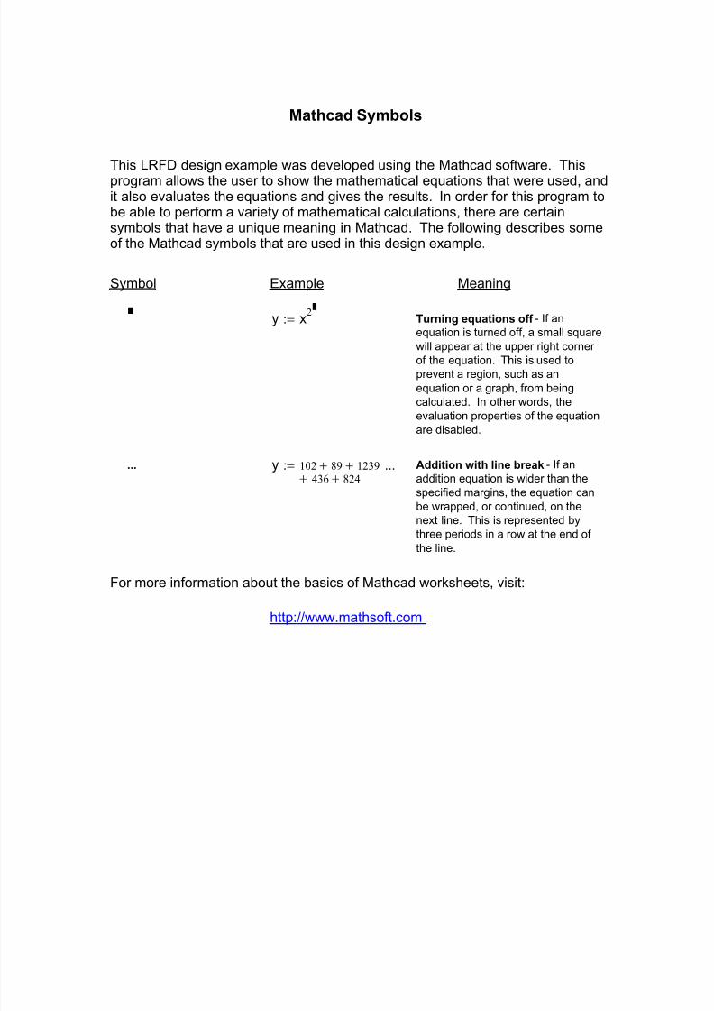
7/29/2019 LRFD steel design.pdf
http://slidepdf.com/reader/full/lrfd-steel-designpdf 48/646
Mathcad Symbols
This LRFD design example was developed using the Mathcad software. This
program allows the user to show the mathematical equations that were used, andit also evaluates the equations and gives the results. In order for this program tobe able to perform a variety of mathematical calculations, there are certainsymbols that have a unique meaning in Mathcad. The following describes someof the Mathcad symbols that are used in this design example.
Symbol Example Meaning
y x2
:= Turning equations off - If an
equation is turned off, a small square
will appear at the upper right corner
of the equation. This is used to
prevent a region, such as an
equation or a graph, from being
calculated. In other words, the
evaluation properties of the equation
are disabled.
... y 102 89+ 1239+
436 824++
...:= Addition with line break - If an
addition equation is wider than the
specified margins, the equation can
be wrapped, or continued, on the
next line. This is represented by
three periods in a row at the end of the line.
For more information about the basics of Mathcad worksheets, visit:
http://www.mathsoft.com

7/29/2019 LRFD steel design.pdf
http://slidepdf.com/reader/full/lrfd-steel-designpdf 49/646
Design Step 1 is the first of several steps that illustrate the designprocedures used for a steel girder bridge. This design step servesas an introduction to this design example and it provides general
information about the bridge design.
Purpose
The purpose of this project is to provide a basic design example for a steel girder bridge as an informational tool for the practicing bridgeengineer. The example is also aimed at assisting the bridgeengineer with the transition from Load Factor Design (LFD) to Loadand Resistance Factor Design (LRFD).
AASHTO References
For uniformity and simplicity, this design example is based on the AASHTO LRFD Bridge Design Specifications (Second Edition,1998, including interims for 1999 through 2002). References to the
AASHTO LRFD Bridge Design Specifications are includedthroughout the design example. AASHTO references are presentedin a dedicated column in the right margin of each page, immediatelyadjacent to the corresponding design procedure. The followingabbreviations are used in the AASHTO references:
Introduction
12Design Step 1.6 - Plan for Bridge Aesthetics
11Design Step 1.5 - Perform Type, Size and Location Study
10Design Step 1.4 - Obtain Geotechnical Recommendations
10Design Step 1.3 - Perform Span Arrangement Study
9Design Step 1.2 - Obtain Geometry Requirements
6Design Step 1.1 - Obtain Design Criteria
1Introduction
PageTable of Contents
General Information / IntroductionDesign Step 1
1-1
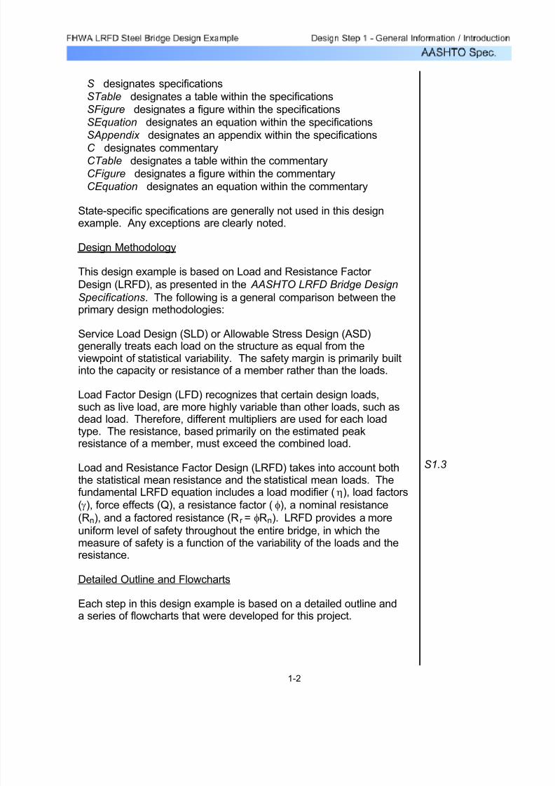
7/29/2019 LRFD steel design.pdf
http://slidepdf.com/reader/full/lrfd-steel-designpdf 50/646
S designates specifications
STable designates a table within the specifications
SFigure designates a figure within the specifications
SEquation designates an equation within the specifications
SAppendix designates an appendix within the specifications C designates commentary
CTable designates a table within the commentary
CFigure designates a figure within the commentary
CEquation designates an equation within the commentary
State-specific specifications are generally not used in this designexample. Any exceptions are clearly noted.
Design Methodology
This design example is based on Load and Resistance Factor Design (LRFD), as presented in the AASHTO LRFD Bridge Design
Specifications. The following is a general comparison between theprimary design methodologies:
Service Load Design (SLD) or Allowable Stress Design (ASD)generally treats each load on the structure as equal from theviewpoint of statistical variability. The safety margin is primarily builtinto the capacity or resistance of a member rather than the loads.
Load Factor Design (LFD) recognizes that certain design loads,such as live load, are more highly variable than other loads, such asdead load. Therefore, different multipliers are used for each loadtype. The resistance, based primarily on the estimated peakresistance of a member, must exceed the combined load.
Load and Resistance Factor Design (LRFD) takes into account boththe statistical mean resistance and the statistical mean loads. Thefundamental LRFD equation includes a load modifier (η), load factors
(γ), force effects (Q), a resistance factor (φ), a nominal resistance
(Rn), and a factored resistance (Rr = φRn). LRFD provides a more
uniform level of safety throughout the entire bridge, in which themeasure of safety is a function of the variability of the loads and theresistance.
Detailed Outline and Flowcharts
Each step in this design example is based on a detailed outline anda series of flowcharts that were developed for this project.
S1.3
1-2
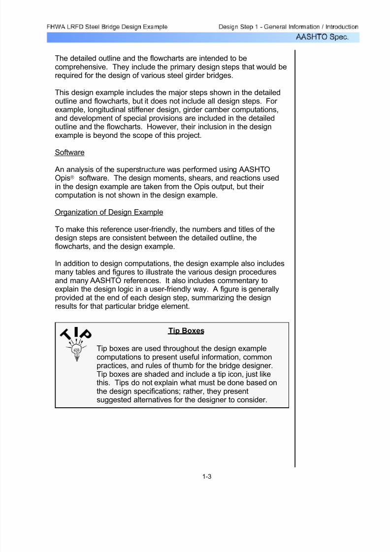
7/29/2019 LRFD steel design.pdf
http://slidepdf.com/reader/full/lrfd-steel-designpdf 51/646
The detailed outline and the flowcharts are intended to becomprehensive. They include the primary design steps that would berequired for the design of various steel girder bridges.
This design example includes the major steps shown in the detailedoutline and flowcharts, but it does not include all design steps. For example, longitudinal stiffener design, girder camber computations,and development of special provisions are included in the detailedoutline and the flowcharts. However, their inclusion in the designexample is beyond the scope of this project.
Software
An analysis of the superstructure was performed using AASHTOOpis software. The design moments, shears, and reactions usedin the design example are taken from the Opis output, but their
computation is not shown in the design example.
Organization of Design Example
To make this reference user-friendly, the numbers and titles of thedesign steps are consistent between the detailed outline, theflowcharts, and the design example.
In addition to design computations, the design example also includesmany tables and figures to illustrate the various design proceduresand many AASHTO references. It also includes commentary to
explain the design logic in a user-friendly way. A figure is generallyprovided at the end of each design step, summarizing the designresults for that particular bridge element.
®
Tip Boxes
Tip boxes are used throughout the design examplecomputations to present useful information, commonpractices, and rules of thumb for the bridge designer.Tip boxes are shaded and include a tip icon, just likethis. Tips do not explain what must be done based onthe design specifications; rather, they presentsuggested alternatives for the designer to consider.
1-3

7/29/2019 LRFD steel design.pdf
http://slidepdf.com/reader/full/lrfd-steel-designpdf 52/646
Design Parameters
The following is a list of parameters upon which this design exampleis based:
1. Two span, square, continuous structure configuration2. Bridge width 44 feet curb to curb (two 12-foot lanes and two
10-foot shoulders)3. Reinforced concrete deck with overhangs4. F-shape barriers (standard design)5. Grade 50 steel throughout6. Opis superstructure design software to be used to generate
superstructure loads7. Nominally stiffened web with no web tapers8. Maximum of two flange transitions top and bottom, symmetric
about pier centerline
9. Composite deck throughout, with one shear connector design/check
10. Constructibility checks based on a single deck pour 11. Girder to be designed with appropriate fatigue categories (to be
identified on sketches)12. No detailed cross-frame design (general process description
provided)13. One bearing stiffener design14. Transverse stiffeners designed as required15. One field splice design (commentary provided on economical
locations)
16. One elastomeric bearing design17. Reinforced concrete cantilever abutments on piles (only one will
be designed, including pile computations)18. One cantilever type wingwall will be designed (all four wingwalls
are similar in height and configuration)19. Reinforced concrete hammerhead pier configuration with pile
foundation
1-4
7/29/2019 LRFD steel design.pdf
http://slidepdf.com/reader/full/lrfd-steel-designpdf 53/646
Summary of Design Steps
The following is a summary of the major design steps included in thisproject:
Design Step 1 - General InformationDesign Step 2 - Concrete Deck DesignDesign Step 3 - Steel Girder DesignDesign Step 4 - Bolted Field Splice DesignDesign Step 5 - Miscellaneous Steel Design
(i.e., shear connectors, bearing stiffeners, and cross frames)Design Step 6 - Bearing DesignDesign Step 7 - Abutment and Wingwall DesignDesign Step 8 - Pier DesignDesign Step 9 - Miscellaneous Design
(i.e., approach slabs, deck drainage, and bridge lighting)Design Step 10 - Special Provisions and Cost EstimateDesign Step P - Pile Foundation Design (part of Design Steps 7 & 8)
To provide a comprehensive summary for general steel bridgedesign, all of the above design steps are included in the detailedoutline and in the flowcharts. However, this design example includesonly those steps that are within the scope of this project. Therefore,Design Steps 1 through 8 are included in the design example, butDesign Steps 9 and 10 are not.
The following units are defined for use in this design example:
K 1000lb= kcf K
ft3
= ksiK
in2
=
1-5

7/29/2019 LRFD steel design.pdf
http://slidepdf.com/reader/full/lrfd-steel-designpdf 54/646
Fu 65ksi= STable 6.4.1-1
Concrete 28-daycompressive strength:
S5.4.2.1f'c 4.0ksi=
Reinforcementstrength: f y 60ksi= S5.4.3 & S6.10.3.7
Steel density: Ws 0.490kcf = STable 3.5.1-1
Concrete density: Wc 0.150kcf = STable 3.5.1-1
Parapet weight (each): Wpar 0.53 Kft
=
Future wearing surface: Wfws 0.140kcf = STable 3.5.1-1
Future wearingsurface thickness: tfws 2.5in= (assumed)
Design Step 1.1 - Obtain Design Criteria
The first step for any bridge design is to establish the design criteria.For this design example, the following is a summary of the primary
design criteria:
Design Criteria
Governing specifications: AASHTO LRFD Bridge Design
Specifications (Second Edition, 1998,including interims for 1999 through2002)
Design methodology: Load and Resistance Factor Design(LRFD)
Live load requirements: HL-93 S3.6
Deck width: wdeck 46.875ft=
Roadway width: wroadway 44.0ft=
Bridge length: Ltotal 240 ft⋅=
Skew angle: Skew 0deg=
Structural steel yieldstrength:
Fy 50ksi= STable 6.4.1-1
Structural steel tensilestrength:
1-6

7/29/2019 LRFD steel design.pdf
http://slidepdf.com/reader/full/lrfd-steel-designpdf 55/646
The following is a summary of other design factors from the
AASHTO LRFD Bridge Design Specifications. Additionalinformation is provided in the Specifications, and specific sectionreferences are provided in the right margin of the design example.
η 1.00=
Therefore for this design example, use:
η 1.00≤andη1
ηD ηR⋅ ηI⋅=
SEquation
1.3.2.1-3
For loads for which the minimum value of γi is appropriate:
η 0.95≥andη ηD ηR⋅ ηI⋅=SEquation
1.3.2.1-2
For loads for which the maximum value of γi is appropriate:
η I 1.0=ηR 1.0=ηD 1.0=
S1.3.2.1The first set of design factors applies to all force effects and isrepresented by the Greek letter η (eta) in the Specifications. These
factors are related to the ductility, redundancy, and operationalimportance of the structure. A single, combined eta is required for
every structure. When a maximum load factor from STable 3.4.1-2 isused, the factored load is multiplied by eta, and when a minimum loadfactor is used, the factored load is divided by eta. All other loads,
factored in accordance with STable 3.4.1-1, are multiplied by eta if amaximum force effect is desired and are divided by eta if a minimumforce effect is desired. In this design example, it is assumed that alleta factors are equal to 1.0.
Design Factors from AASHTO LRFD Bridge Design Specifications
1-7
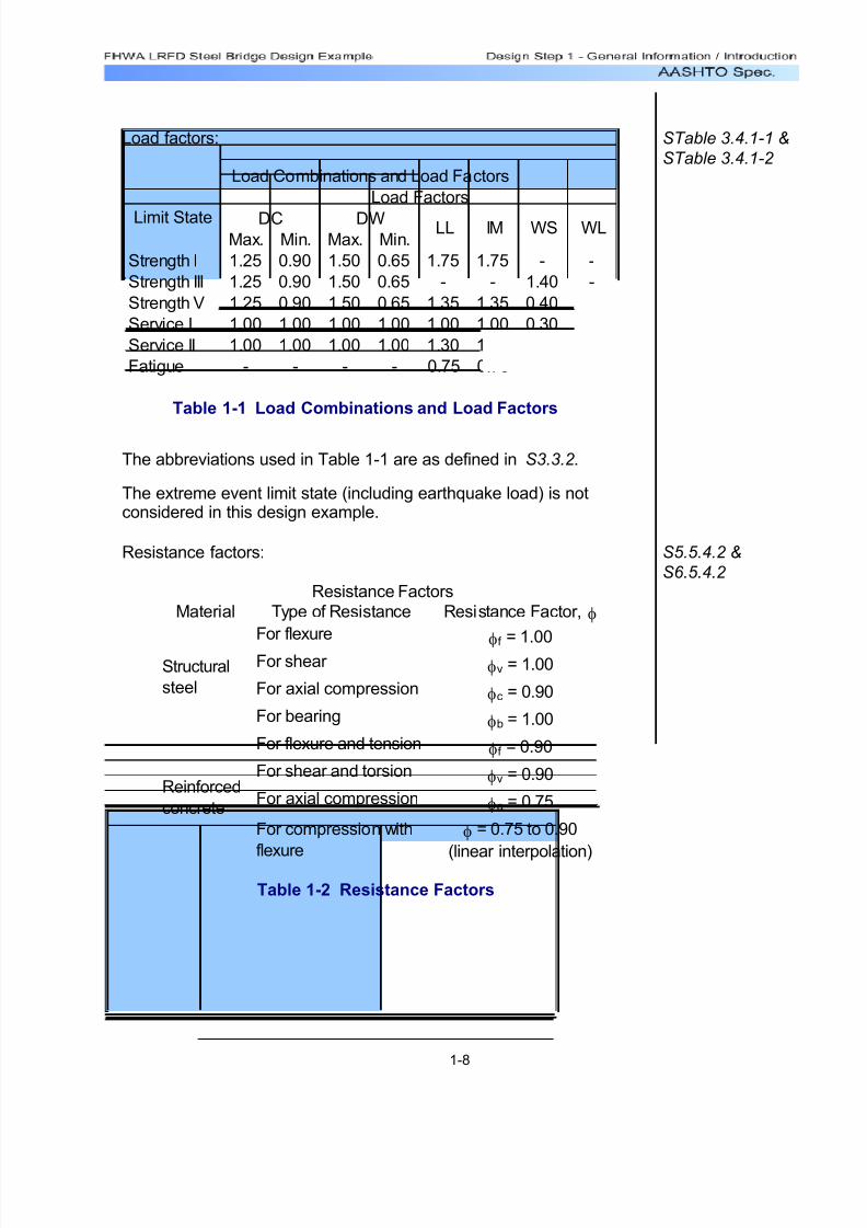
7/29/2019 LRFD steel design.pdf
http://slidepdf.com/reader/full/lrfd-steel-designpdf 56/646
Load factors: STable 3.4.1-1 &
STable 3.4.1-2
Max. Min. Max. Min.
Strength I 1.25 0.90 1.50 0.65 1.75 1.75 - -
Strength III 1.25 0.90 1.50 0.65 - - 1.40 -
Strength V 1.25 0.90 1.50 0.65 1.35 1.35 0.40 1.00
Service I 1.00 1.00 1.00 1.00 1.00 1.00 0.30 1.00
Service II 1.00 1.00 1.00 1.00 1.30 1.30 - -
Fatigue - - - - 0.75 0.75 - -
Load Combinations and Load Factors
Load Factors
Limit State DC DW LL IM WS WL
Table 1-1 Load Combinations and Load Factors
The abbreviations used in Table 1-1 are as defined in S3.3.2 .
The extreme event limit state (including earthquake load) is notconsidered in this design example.
Resistance factors: S5.5.4.2 &
S6.5.4.2
Material Type of Resistance Resistance Factor, φ
For flexureφf = 1.00
For shear φv = 1.00
For axial compression φc = 0.90
For bearing φb = 1.00
For flexure and tension φf = 0.90
For shear and torsion φv = 0.90
For axial compression φa = 0.75
For compression with
flexureφ = 0.75 to 0.90
(linear interpolation)
Resistance Factors
Structural
steel
Reinforced
concrete
Table 1-2 Resistance Factors
1-8
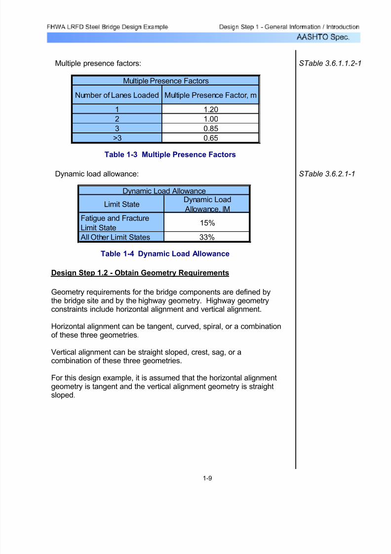
7/29/2019 LRFD steel design.pdf
http://slidepdf.com/reader/full/lrfd-steel-designpdf 57/646
Multiple presence factors: STable 3.6.1.1.2-1
Number of Lanes Loaded Multiple Presence Factor, m
1 1.20
2 1.00
3 0.85
>3 0.65
Multiple Presence Factors
Table 1-3 Multiple Presence Factors
Dynamic load allowance: STable 3.6.2.1-1
Fatigue and Fracture
Limit State15%
All Other Limit States 33%
Dynamic Load AllowanceDynamic Load
Allowance, IMLimit State
Table 1-4 Dynamic Load Allowance
Design Step 1.2 - Obtain Geometry Requirements
Geometry requirements for the bridge components are defined bythe bridge site and by the highway geometry. Highway geometryconstraints include horizontal alignment and vertical alignment.
Horizontal alignment can be tangent, curved, spiral, or a combinationof these three geometries.
Vertical alignment can be straight sloped, crest, sag, or acombination of these three geometries.
For this design example, it is assumed that the horizontal alignment
geometry is tangent and the vertical alignment geometry is straightsloped.
1-9

7/29/2019 LRFD steel design.pdf
http://slidepdf.com/reader/full/lrfd-steel-designpdf 58/646
Design Step 1.3 - Perform Span Arrangement Study
Some clients require a Span Arrangement Study. The Span Arrangement Study includes selecting the bridge type, determining
the span arrangement, determining substructure locations, computingspan lengths, and checking horizontal clearance for the purpose of approval.
Although a Span Arrangement Study may not be required by theclient, these determinations must still be made by the engineer beforeproceeding to the next design step.
For this design example, the span arrangement is presented inFigure 1-1. This span arrangement was selected to illustrate variousdesign criteria and the established geometry constraints identified for
this example.
120'-0” 120'-0”
240'-0”
L Bearings
Abutment 1
L Bearings
Abutment 2L Pier
EFE
Legend:
E = Expansion Bearings
F = Fixed Bearings
CC
C
Figure 1-1 Span Arrangement
Design Step 1.4 - Obtain Geotechnical Recommendations
The subsurface conditions must be determined to developgeotechnical recommendations.
Subsurface conditions are commonly determined by taking coreborings at the bridge site. The borings provide a wealth of information about the subsurface conditions, all of which is recorded
in the boring logs.
It is important to note that the boring log reveals the subsurfaceconditions for a finite location and not necessarily for the entirebridge site. Therefore, several borings are usually taken at eachproposed substructure location. This improves their reliability as areflection of subsurface conditions at the bridge site, and it allowsthe engineer to compensate for significant variations in thesubsurface profile.
1-10

7/29/2019 LRFD steel design.pdf
http://slidepdf.com/reader/full/lrfd-steel-designpdf 59/646
After the subsurface conditions have been explored anddocumented, a geotechnical engineer must develop foundation typerecommendations for all substructures. Foundations can be spreadfootings, pile foundations, or drilled shafts. Geotechnicalrecommendations typically include allowable bearing pressure,allowable settlement, and allowable pile resistances (axial andlateral), as well as required safety factors for overturning and sliding.
For this design example, pile foundations are used for allsubstructure units.
Design Step 1.5 - Perform Type, Size and Location Study
Some clients require a Type, Size and Location study for the purposeof approval. The Type, Size and Location study includes preliminaryconfigurations for the superstructure and substructure componentsrelative to highway geometry constraints and site conditions. Detailsof this study for the superstructure include selecting the girder types,determining the girder spacing, computing the approximate requiredgirder span and depth, and checking vertical clearance.
Although a Type, Size and Location study may not be required by theclient, these determinations must still be made by the engineer beforeproceeding to the next design step.
For this design example, the superstructure cross section ispresented in Figure 1-2. This superstructure cross section was
selected to illustrate selected design criteria and the establishedgeometry constraints. When selecting the girder spacing,consideration was given to half-width deck replacement.
3'-6” (Typ.)
3'-11¼" 3'-11¼"
10'-0”
Shoulder
4 Spaces @ 9’-9” = 39’-0”
1'-5¼"12'-0”
Lane
12'-0”
Lane
10'-0”
Shoulder
46'-10½"
Figure 1-2 Superstructure Cross Section
1-11

7/29/2019 LRFD steel design.pdf
http://slidepdf.com/reader/full/lrfd-steel-designpdf 60/646
Design Step 1.6 - Plan for Bridge Aesthetics
Finally, the bridge engineer must consider bridge aestheticsthroughout the design process. Special attention to aesthetics should
be made during the preliminary stages of the bridge design, beforethe bridge layout and appearance has been fully determined.
To plan an aesthetic bridge design, the engineer must consider thefollowing parameters:
Function: Aesthetics is generally enhanced when form follows•function.Proportion: Provide balanced proportions for members and span•lengths.Harmony: The parts of the bridge must usually complement each•
other, and the bridge must usually complement its surroundings.Order and rhythm: All members must be tied together in an orderly•manner.Contrast and texture: Use textured surfaces to reduce visual mass.•Light and shadow: Careful use of shadow can give the bridge a•more slender appearance.
1-12

7/29/2019 LRFD steel design.pdf
http://slidepdf.com/reader/full/lrfd-steel-designpdf 61/646
Design Step 2.10 - Design for Negative Flexure in Deck 21
Design Step 2.11 - Check for Negative Flexure Cracking under Service Limit State
22
Design Step 2.12 - Design for Flexure in Deck Overhang 25
Design Step 2.13 - Check for Cracking in Overhang under Service Limit State
42
Design Step 2.14 - Compute Overhang Cut-off LengthRequirement
43
Design Step 2.15 - Compute Overhang Development Length 44
Design Step 2.16 - Design Bottom Longitudinal DistributionReinforcement
46
Design Step 2.17 - Design Top Longitudinal DistributionReinforcement
47
Design Step 2.18 - Design Longitudinal Reinforcement over
Piers
49
Design Step 2.19 - Draw Schematic of Final ConcreteDeck Design
51
Concrete Deck Design ExampleDesign Step 2
Table of Contents
Page
Design Step 2.1 - Obtain Design Criteria 2
Design Step 2.2 - Determine Minimum Slab Thickness 5
Design Step 2.3 - Determine Minimum Overhang Thickness 5
Design Step 2.4 - Select Slab and Overhang Thickness 5
Design Step 2.5 - Compute Dead Load Effects 5
Design Step 2.6 - Compute Live Load Effects 7
Design Step 2.7 - Compute Factored Positive and NegativeDesign Moments
9
Design Step 2.8 - Design for Positive Flexure in Deck 15
Design Step 2.9 - Check for Positive Flexure Cracking under Service Limit State
17
2-1
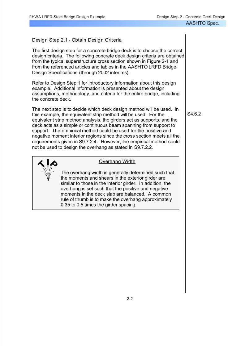
7/29/2019 LRFD steel design.pdf
http://slidepdf.com/reader/full/lrfd-steel-designpdf 62/646
Design Step 2.1 - Obtain Design Criteria
The first design step for a concrete bridge deck is to choose the correctdesign criteria. The following concrete deck design criteria are obtained
from the typical superstructure cross section shown in Figure 2-1 andfrom the referenced articles and tables in the AASHTO LRFD Bridge
Design Specifications (through 2002 interims).
Refer to Design Step 1 for introductory information about this designexample. Additional information is presented about the designassumptions, methodology, and criteria for the entire bridge, includingthe concrete deck.
The next step is to decide which deck design method will be used. Inthis example, the equivalent strip method will be used. For the
equivalent strip method analysis, the girders act as supports, and thedeck acts as a simple or continuous beam spanning from support tosupport. The empirical method could be used for the positive andnegative moment interior regions since the cross section meets all the
requirements given in S9.7.2.4. However, the empirical method could
not be used to design the overhang as stated in S9.7.2.2.
S4.6.2
Overhang Width
The overhang width is generally determined such thatthe moments and shears in the exterior girder are
similar to those in the interior girder. In addition, theoverhang is set such that the positive and negativemoments in the deck slab are balanced. A commonrule of thumb is to make the overhang approximately0.35 to 0.5 times the girder spacing.
2-2
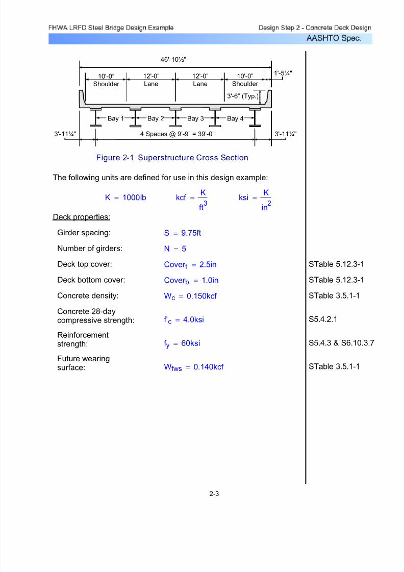
7/29/2019 LRFD steel design.pdf
http://slidepdf.com/reader/full/lrfd-steel-designpdf 63/646
STable 3.5.1-1Wfws 0.140kcf =Future wearingsurface:
S5.4.3 & S6.10.3.7f y 60ksi=Reinforcementstrength:
S5.4.2.1f'c 4.0ksi=Concrete 28-daycompressive strength:
STable 3.5.1-1Wc
0.150kcf =Concrete density:
STable 5.12.3-1Cover b 1.0in=Deck bottom cover:
STable 5.12.3-1Cover t 2.5in=Deck top cover:
N 5=Number of girders:
S 9.75ft=Girder spacing:
Deck properties:
ksi
K
in2=kcf
K
ft3=K 1000lb=
The following units are defined for use in this design example:
Figure 2-1 Superstructure Cross Section
3'-6” (Typ.)
3'-11¼" 3'-11¼"
10'-0”Shoulder
4 Spaces @ 9’-9” = 39’-0”
1'-5¼"12'-0”Lane
12'-0”Lane
10'-0”Shoulder
46'-10½"
Bay 1 Bay 2 Bay 3 Bay 4
2-3

7/29/2019 LRFD steel design.pdf
http://slidepdf.com/reader/full/lrfd-steel-designpdf 64/646
STable 3.5.1-1Future wearing surface density - The future wearing surface
density is 0.140 KCF. A 2.5 inch thickness will be assumed.
STable C5.4.2.1-1
S5.4.2.1Concrete 28-day compressive strength - The compressive strength
for decks shall not be less than 4.0 KSI. Also, type "AE" concreteshould be specified when the deck will be exposed to deicing salts or the freeze-thaw cycle. "AE" concrete has a compressive strength of
4.0 KSI.
STable 5.12.3-1Deck bot tom cover - The concrete bottom cover is set at 1.0 inch
since the bridge deck will use reinforcement that is smaller than a #11bar.
STable 5.12.3-1Deck top cover - The concrete top cover is set at 2.5 inches since the
bridge deck may be exposed to deicing salts and/or tire stud or chain
wear. This includes the 1/2 inch integral wearing surface that isrequired.
* Based on parapet properties not included in this design example.See Publication Number FHWA HI-95-017, Load and ResistanceFactor Design for Highway Bridges, Participant Notebook, Volume II(Version 3.01), for the method used to compute the parapet properties.
SA13.3.1(calculated inDesign Step 2.12)Rw 117.40K=
Total transverse
resistance of the parapet*:
SA13.3.1(calculated inDesign Step 2.12)
Lc 12.84ft=Critical length of yieldline failure pattern*:
Hpar 3.5ft=Parapet height:
Mco 28.21K ft⋅
ft=
Moment capacityat base*:
wbase 1.4375ft=Width at base:
Wpar 0.53K
ft=Weight per foot:
Parapet properties:
2-4

7/29/2019 LRFD steel design.pdf
http://slidepdf.com/reader/full/lrfd-steel-designpdf 65/646
γpDWmin 0.65=Minimum
γpDWmax 1.50=Maximum
For future wearing surface:
γpDCmin 0.90=Minimum
γpDCmax
1.25=Maximum
For slab and parapet:
STable 3.4.1-2 After the dead load moments are computed for the slab, parapets, andfuture wearing surface, the correct load factors must be identified. Theload factors for dead loads are:
STable 3.5.1-1The next step is to compute the dead load moments. The dead loadmoments for the deck slab, parapets, and future wearing surface are
tabulated in Table 2-1. The tabulated moments are presented for tenthpoints for Bays 1 through 4 for a 1-foot strip. The tenth points arebased on the equivalent span and not the center-to-center beamspacing.
Design Step 2.5 - Compute Dead Load Effects
to 9.0in=and ts 8.5in=
Design Step 2.4 - Select Slab and Overhang Thickness
Once the minimum slab and overhang thicknesses are computed, they
can be increased as needed based on client standards and designcomputations. The following slab and overhang thicknesses will beassumed for this design example:
to 8.0in=
S13.7.3.1.2For concrete deck overhangs supporting concrete parapets or barriers,the minimum deck overhang thickness is:
Design Step 2.3 - Determine Minimum Overhang Thickness
S9.7.1.1
Design Step 2.2 - Determine Minimum Slab Thickness
The concrete deck depth cannot be less than 7.0 inches, excludingany provision for grinding, grooving, and sacrificial surface.
2-5

7/29/2019 LRFD steel design.pdf
http://slidepdf.com/reader/full/lrfd-steel-designpdf 66/646
1 . 0
- 0 . 7 1
- 0 . 7 2
- 0 . 7 1
- 0 . 7 4
0 . 4
3
- 0 . 2 3
0 . 4
7
- 1 . 6 6
- 0 . 2 4
- 0 . 1 8
- 0 . 2 4
- 0 . 0 6
0 . 9
- 0 . 3 0
- 0 . 3 1
- 0 . 3 0
- 0 . 3 3
0 . 2 2
- 0 . 1 6
0 . 4 0
- 1 . 4 5
- 0 . 1 1
- 0 . 0 7
- 0 . 1 2
0 . 0 4
0 . 8
0 . 0 1
0 . 0 1
0 . 0 2
- 0 . 0 1
0 . 0 2
- 0 . 0 9
0 . 3 3
- 1 . 2 4
0 . 0 0
0 . 0 1
- 0 . 0 2
0 . 1 1
0 . 7
0 . 2 4
0 . 2 4
0 . 2 4
0 . 2 2
- 0 . 1 9
- 0 . 0 2
0 . 2 6
- 1 . 0 3
0 . 0 8
0 . 0 7
0 . 0 5
0 . 1 5
0 . 6
0 . 3 7
0 . 3 8
0 . 3 8
0 . 3 6
- 0 .
4 0
0 . 0 5
0 . 1 9
- 0 .
8 2
0 . 1 4
0 . 1 0
0 . 0 9
0 . 1 7
0 . 5
0 . 4 1
0 . 4 2
0 . 4 2
0 . 4 1
- 0 . 6 1
0 . 1 2
0 . 1 2
- 0 . 6 1
0 . 1 7
0 . 1 1
0 . 1 1
0 . 1 7
0 . 4
0 . 3 6
0 . 3 8
0 . 3 8
0 . 3 7
- 0 . 8 2
0 . 1 9
0 . 0 5
- 0 . 4 0
0 . 1 7
0 . 0 9
0 . 1 0
0 . 1 4
0 . 3
0 . 2 2
0 . 2 4
0 . 2 4
0 . 2 4
- 1 . 0 3
0 . 2 6
- 0 . 0 2
- 0 . 1 9
0 . 1 5
0 . 0 5
0 . 0 7
0 . 0 8
0
. 2
- 0 . 0 1
0 . 0 2
0 . 0 1
0 . 0 1
- 1 . 2 4
0 . 3 3
- 0 . 0 9
0 . 0 2
0 . 1 1
- 0 . 0 2
0 . 0 1
0 . 0 0
0 . 1
- 0 . 3 3
- 0 . 3 0
- 0 . 3 1
- 0 . 3 0
- 1 . 4 5
0 . 4 0
- 0 . 1 6
0 . 2 2
0 . 0 4
- 0 . 1 2
- 0 . 0 7
- 0 . 1 1
0 . 0
- 0 . 7 4
- 0 . 7 1
- 0 . 7 2
- 0 . 7 1
- 1 . 6 6
0 . 4 7
- 0 . 2 3
0 . 4 3
- 0 . 0 6
- 0 . 2 4
- 0 . 1 8
- 0 . 2 4
D I S T A N C E
B A Y 1
B A Y 2
B A Y 3
B A Y 4
B A Y 1
B A Y 2
B A Y 3
B A Y 4
B A Y 1
B A Y 2
B A Y 3
B A Y 4
T a b l e 2 - 1
U n f a c t o
r e d D e a d L o a d M o m e n t s ( K - F T / F T )
S L A B D E A D
L O A D
P A R A P E T
D E A D
L O A D
F W S D E A D
L O A D
2-6

7/29/2019 LRFD steel design.pdf
http://slidepdf.com/reader/full/lrfd-steel-designpdf 67/646
Based on the above information and based on S4.6.2.1, the live loadeffects for one and two trucks are tabulated in Table 2-2. The live loadeffects are given for tenth points for Bays 1 through 4. Multiplepresence factors are included, but dynamic load allowance is excluded.
S1.3.2.1φext 1.00=Extreme event limit state
S1.3.2.1φserv 1.00=Service limit state
S5.5.4.2φstr 0.90=Strength limit state
Resistance factors for flexure:
S9.5.3 & S5.5.3.1Fatigue does not need to be investigated for concrete deck design .
STable 3.6.1.1.2-1Multiple presence factor, m:
With one lane loaded, m = 1.20With two lanes loaded, m = 1.00With three lanes loaded, m = 0.85
STable 3.4.1-1γLL 1.75=Load factor for live load - Strength I
STable 3.6.2.1-1IM 0.33=Dynamic load allowance, IM
S3.6.1.3.1The minimum distance between the wheels of two adjacent designvehicles = 4 feet
S3.6.1.3.1The minimum distance from the center of design vehicle wheel tothe inside face of parapet = 1 foot
Design Step 2.6 - Compute Live Load Effects
Before the live load effects can be computed, the following basicparameters must be defined:
2-7

7/29/2019 LRFD steel design.pdf
http://slidepdf.com/reader/full/lrfd-steel-designpdf 68/646
1 . 0 4 . 5 5
5 . 8 2
4 . 0 7
3 . 6 2
- 2 8 . 5 1
- 2 7 . 1 2
- 2 8 . 3 7
- 0 . 4 4
2 . 2 8
- 2 . 8 7
2 . 2 8
2 . 6 6
- 2 9 . 3 9
- 2 7 . 9 4
- 2 8 . 8 3
- 0 . 2 7
0 . 9 5 . 6 8
6 . 0 1
7 . 8 4
1 7 . 0 3
- 1 5 . 1 1
- 1 5 . 8 4
- 1 9 . 1 0
- 2 . 0 8
2 . 0 6
7 . 1 9
8 . 0 4
1 2 . 4 9
- 1 8 . 3 2
- 1 7 . 3 7
- 1 4 . 4 4
- 1 . 2 6
0 . 8
1 8 . 1 0
1 8 . 3 5
2 0 . 6 8
3 0 . 4 3
- 1 3 . 4 8
- 1 3 . 6 3
- 1 6 . 3 9
- 3 . 7 0
4 . 5 0
1 5 . 1 4
1 6 . 9 8
2 2 . 3 2
- 8 . 1 8
- 8 . 0 1
- 2 . 1 0
- 2 . 2 5
0 . 7
2 7 . 1 3
2 7 . 2 0
2 5 . 3 9
3 6 . 6 4
- 1 1 . 8 4
- 1 1 . 4 1
- 1 3 . 6 8
- 5 . 3 3
1 4 . 0 0
2 0 . 4 8
1 9 . 1 5
2 6 . 4 6
- 7 . 1 9
- 5 . 7 4
- 1 . 4 4
- 3 . 2 4
0 . 6
3 2 . 4 8
2 8 . 0 0
2 9 . 2 8
3 6 . 6 2
- 1 0 . 2 2
- 9 . 2 0
- 1 0 . 9 7
- 6 . 9 6
2 1 . 2 1
1 9 . 5 8
2 1 . 3 0
2 5 . 8 4
- 6 . 2 0
- 4 . 6 2
- 2 . 6 8
- 4 . 2 2
0 . 5 3 1 . 2
0
2 8 . 2
6
2 8 . 1
4
3 1 . 1
0
- 8 . 5
9
- 8 . 5
7
- 8 . 2
7
- 8 . 5
9
2 1 . 0
1
2 1 . 7
2
2 1 . 6
4
2 0 . 9
3
- 5 . 2
1
- 3 . 5
1
- 3 . 9
2
- 5 . 2
1
0 . 4
3 6 . 7 6
2 9 . 0 9
2 8 . 1 4
2 6 . 1 4
- 6 . 9 6
- 1 1 . 3 8
- 9 . 2 0
- 1 0 . 2 2
2 5 . 9 3
2 1 . 1 9
1 9 . 4 1
1 7 . 9 6
- 4 . 2 3
- 2 . 4 0
- 5 . 1 7
- 6 . 2 0
0 . 3
3 6 . 4 4
2 5 . 5 6
2 7 . 3 7
1 6 . 1 9
- 5 . 3 3
- 1 4 . 1 8
- 1 1 . 4 2
- 1 1 . 8 4
2 6 . 3 5
1 9 . 2 6
1 6 . 7 1
1 0 . 4 8
- 3 . 2 4
- 1 . 2 9
- 6 . 4 1
- 7 . 1 9
0 . 2
3 0 . 5 3
2 0 . 8 8
1 8 . 2 2
1 1 . 6 6
- 3 . 7 0
- 1 7 . 0 0
- 1 3 . 6 3
- 1 3 . 4 8
2 2 . 3 6
1 7 . 1 0
7 . 7 3
4 . 5 9
- 2 . 7 1
- 8 . 5 3
- 8 . 0 2
- 8 . 1 8
0
. 1
2 2
. 9 4
7 . 7 3
6 . 2 2
5 . 5 6
- 1 4 . 4 5
- 1 9 . 8 1
- 1 5 . 8 5
- 1 5 . 1 1
1 7
. 4 4
7 . 9 8
7 . 3 2
2 . 3 0
- 1 2 . 0 9
- 1 6 . 9 2
- 1 7 . 3 8
- 1 8 . 3 3
0 . 0 5 . 6 2
4 . 0 7
6 . 0 4
4 . 5 5
- 2 5 . 7 5
- 2 8 . 3 8
- 2 7 . 1 3
- 2 8 . 5 1
4 . 3 6
2 . 0 4
- 2 . 9 2
2 . 5 5
- 2 1 . 4 7
- 2 9 . 3 6
- 2 7 . 9 2
- 2 9 . 4 0
D I S T A N C E
B A Y 1
B A Y 2
B A Y 3
B A Y 4
B A Y 1
B A Y 2
B A Y 3
B A Y 4
B A Y 1
B A Y 2
B A Y 3
B A Y 4
B A Y 1
B A Y 2
B A Y 3
B A Y 4
T a b l e 2
- 2
U n f a c t o r e d L i v e L o a d M o
m e n t s ( E x c l u d i n g D y n a m i c L
o a d A l l o w a n c e ) ( K - F T )
S I N G L E T R U C K
( M U L T I P L E
P R E S E N C E
F A C T O R O F 1 . 2 0
I N C L U D E D )
T W O T R U C K S
( M U L T I P L E
P R E S E N C E
F A C T O R O F 1 . 0 0
I N C L U D E D )
M A X .
M O M E N T
M I N .
M O M E N T
M A X .
M O M E N T
M I N .
M O M E N T
2-8

7/29/2019 LRFD steel design.pdf
http://slidepdf.com/reader/full/lrfd-steel-designpdf 69/646
Design Step 2.7 - Compute Factored Posi tive and Negative
Design Moments
For this example, the design moments will be computed two differentways.
For Method A, the live load portion of the factored design moments willbe computed based on the values presented in Table 2-2. Table 2-2represents a continuous beam analysis of the example deck using afinite element analysis program.
For Method B, the live load portion of the factored design moments will
be computed using STable A4.1-1. In STable A4.1-1, moments per unit width include dynamic load allowance and multiple presencefactors. The values are tabulated using the equivalent strip method for
various bridge cross sections. The values in STable A4.1-1 may beslightly higher than the values from a deck analysis based on the actualnumber of beams and the actual overhang length. The maximum liveload moment is obtained from the table based on the girder spacing.For girder spacings between the values listed in the table, interpolationcan be used to get the moment.
STable A4.1-1
Based on Design Step 1, the load modifier eta (η) is 1.0 and will not be
shown throughout the design example. Refer to Design Step 1 for adiscussion of eta.
S1.3.2.1
Factored Positive Design Moment Using Table 2-2 - Method A
Factored positive live load moment:
The positive, negative, and overhang moment equivalent stripequations are presented in Figure 2-2 below.
Negative Moment
= 48.0 + 3.0S
Overhang Moment
= 45.0 + 10.0X
Positive Moment
= 26.0 + 6.6SSTable 4.6.2.1.3-1
Figure 2-2 Equivalent Strip Equations for Various Parts of the
Deck
2-9
7/29/2019 LRFD steel design.pdf
http://slidepdf.com/reader/full/lrfd-steel-designpdf 70/646
It should be noted that the total maximum factored positive moment iscomprised of the maximum factored positive live load moment in Bay 1at 0.4S and the maximum factored positive dead load moment in Bay 2at 0.4S. Summing the factored moments in different bays gives aconservative result. The exact way to compute the maximum totalfactored design moment is by summing the dead and live load momentsat each tenth point per bay. However, the method presented here is asimpler and slightly conservative method of finding the maximum totalfactored moment.
MupostotalA 12.21K ft⋅
ft=
MupostotalA MuposliveA Muposdead+=
The total factored positive design moment for Method A is:
Muposdead 0.85K ft⋅
ft=
Muposdead γpDCmax 0.38K ft⋅
ft⋅⎛
⎝ ⎞ ⎠
⋅ γpDCmax 0.19K ft⋅
ft⋅⎛
⎝ ⎞ ⎠
⋅+
γpDWmax 0.09 K ft⋅ft
⋅⎛ ⎝
⎞ ⎠
⋅+
...=
Based on Table 2-1, the maximum unfactored slab, parapet, and futurewearing surface positive dead load moment occurs in Bay 2 at adistance of 0.4S. The maximum factored positive dead load moment isas follows:
Factored positive dead load moment:
MuposliveA 11.36 K ft⋅ft
=
MuposliveA γLL 1 IM+( )⋅36.76K ft⋅
wposstripa⋅=
Based on Table 2-2, the maximum unfactored positive live loadmoment is 36.76 K-ft, located at 0.4S in Bay 1 for a single truck. Themaximum factored positive live load moment is:
wposstripa 7.53ft=or wposstripa 90.35in=
ftS 9.75=For
wposstripa 26.0 6.6S+=
STable 4.6.2.1.3-1The width of the equivalent strip for positive moment is:
2-10
7/29/2019 LRFD steel design.pdf
http://slidepdf.com/reader/full/lrfd-steel-designpdf 71/646
Method A or Method B
It can be seen that the tabulated values based onSTable A4.1-1 (Method B) are slightly greater than thecomputed live load values using a finite elementanalysis program (Method A). For real world deckdesign, Method B would be preferred over Method Adue to the amount of time that would be saved by nothaving to develop a finite element model. Since thetime was spent to develop the finite element model for this deck design, the Method A values will be used.
MupostotalB MupostotalA−
MupostotalB3.4%=
Comparing Methods A and B, the difference between the total factoreddesign moment for the two methods is:
MupostotalB
12.64K ft⋅
ft=
MupostotalB MuposliveB Muposdead+=
The total factored positive design moment for Method B is:
Muposdead 0.85K ft⋅
ft=
The factored positive dead load moment for Method B is the same asthat for Method A:
Factored positive dead load moment:
MuposliveB 11.80K ft⋅
ft=
MuposliveB γLL 6.74⋅K ft⋅
ft=
This moment is on a per foot basis and includes dynamic loadallowance. The maximum factored positive live load moment is:
STable A4.1-1For a girder spacing of 9'-9", the maximum unfactored positive live loadmoment is 6.74 K-ft/ft.
Factored positive live load moment:
Factored Posit ive Design Moment Using STable A4.1-1 - Method B
2-11

7/29/2019 LRFD steel design.pdf
http://slidepdf.com/reader/full/lrfd-steel-designpdf 72/646
wnegstripa 6.44ft=or wnegstripa 77.25in=
wnegstripa 48.0 3.0S+=
STable 4.6.2.1.3-1The width of the equivalent strip for negative moment is:
1
4bf 0.25ft=
bf 1.0ft= Assume
Figure 2-3 Location of Design Section
S4.6.2.1.6L webC
¼ bf
Design
section
bf
S4.6.2.1.6The deck design section for a steel beam for negative momentsand shear forces is taken as one-quarter of the top flange widthfrom the centerline of the web.
Factored negative live load moment:
Factored Negative Design Moment Using Table 2-2 - Method A
2-12

7/29/2019 LRFD steel design.pdf
http://slidepdf.com/reader/full/lrfd-steel-designpdf 73/646
Based on Table 2-2, the maximum unfactored negative live loadmoment is -29.40 K-ft, located at 0.0S in Bay 4 for two trucks. Themaximum factored negative live load moment is:
MunegliveA γLL 1 IM+( )⋅ 29.40− K ft⋅wnegstripa
⋅=
MunegliveA 10.63−K ft⋅
ft=
Factored negative dead load moment:
From Table 2-1, the maximum unfactored negative dead load momentoccurs in Bay 4 at a distance of 1.0S. The maximum factored negativedead load moment is as follows:
Munegdead γpDCmax 0.74−K ft⋅
ft⋅⎛
⎝ ⎞ ⎠
⋅
γpDCmax 1.66−K ft⋅
ft⋅⎛
⎝ ⎞ ⎠
⋅+
...
γpDWmax 0.06−K ft⋅
ft⋅⎛
⎝ ⎞ ⎠
⋅+
...
=
Munegdead 3.09−K ft⋅
ft=
The total factored negative design moment for Method A is:
MunegtotalA MunegliveA Munegdead+=
MunegtotalA 13.72−K ft⋅
ft=
Factored Negative Design Moment Using STable A4.1-1 - Method B
Factored negative live load moment:
For a girder spacing of 9'-9" and a 3" distance from the centerline of girder to the design section, the maximum unfactored negative live loadmoment is 6.65 K-ft/ft.
STable A4.1-1
If the distance from the centerline of the girder to the design sectiondoes not match one of the distances given in the table, the designmoment can be obtained by interpolation. As stated earlier, thesemoments are on a per foot basis and include dynamic load allowance.
2-13

7/29/2019 LRFD steel design.pdf
http://slidepdf.com/reader/full/lrfd-steel-designpdf 74/646
The maximum factored negative live load moment is:
MunegliveB γLL 6.65−⋅K ft⋅
ft=
MunegliveB 11.64−K ft⋅
ft=
Factored negative dead load moment:
The factored negative dead load moment for Method B is the same asthat for Method A:
Munegdead 3.09−K ft⋅
ft
=
The total factored negative design moment for Method B is:
MunegtotalB MunegliveB Munegdead+=
MunegtotalB 14.73−K ft⋅
ft=
Comparing Methods A and B, the difference between the total factoreddesign moment for the two methods is:
MunegtotalB MunegtotalA−
MunegtotalB6.8%=
Method A or Method B
It can be seen that the tabulated values based on
STable A4.1-1 (Method B) are slightly greater than thecomputed live load values using a finite element
analysis program (Method A). For real world deckdesign, Method B would be preferred over Method Adue to the amount of time that would be saved by nothaving to develop a finite element model. Since thetime was spent to develop the finite element model for this deck design, the Method A values will be used.
2-14
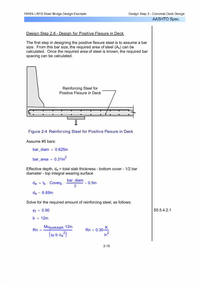
7/29/2019 LRFD steel design.pdf
http://slidepdf.com/reader/full/lrfd-steel-designpdf 75/646
Design Step 2.8 - Design for Posit ive Flexure in Deck
The first step in designing the positive flexure steel is to assume a bar size. From this bar size, the required area of steel (As) can becalculated. Once the required area of steel is known, the required bar spacing can be calculated.
Reinforcing Steel for
Positive Flexure in Deck
Figure 2-4 Reinforcing Steel for Positive Flexure in Deck
Assume #5 bars:
bar_diam 0.625in=
bar_area 0.31in2=
Effective depth, de = total slab thickness - bottom cover - 1/2 bar diameter - top integral wearing surface
de ts Cover b−bar_diam
2− 0.5in−=
de 6.69in=
Solve for the required amount of reinforcing steel, as follows:
φf 0.90= S5.5.4.2.1
b 12in=
RnMupostotalA 12⋅ in
φf b⋅ de2⋅( )
= Rn 0.30K
in2
=
2-15
7/29/2019 LRFD steel design.pdf
http://slidepdf.com/reader/full/lrfd-steel-designpdf 76/646
OK0.12 0.42≤
S5.7.3.3.1c
de0.42≤where
c
de0.12=
S5.7.2.2c 0.80in=ca
β1
=
S5.7.2.2β1 0.85=
a 0.68 in=aT
0.85 f'c
⋅ bar_space⋅=
T 18.60K=T bar_area f y⋅=
S5.7.3.3.1Once the bar size and spacing are known, the maximum reinforcement
limit must be checked.
bar_space 8.0in=Use #5 bars @
Required bar spacing =bar_area
As8.7in=
As 0.43in
2
ft= As ρ
b
ft⋅ de⋅=
Note: The above two equations are derived formulas that can be foundin most reinforced concrete textbooks.
ρ 0.00530=
ρ 0.85f'c
f y
⎛
⎝
⎞
⎠1.0 1.0
2 Rn⋅( )
0.85 f'c⋅( )−−⎡
⎣
⎤
⎦⋅=
2-16

7/29/2019 LRFD steel design.pdf
http://slidepdf.com/reader/full/lrfd-steel-designpdf 77/646
f sa 36.00ksi=Use
0.6f y 36.00ksi=f sa 43.04ksi=
f sa 0.6 f y⋅≤wheref sa
Z
dc Ac⋅( )
1
3
=
The equation that gives the allowable reinforcement service load stressfor crack control is:
Ac 21.00in2=
Ac 2 dc( )⋅ bar_space⋅=
Concrete area with centroid the same astransverse bar and bounded by the crosssection and line parallel to neutral axis:
dc 1.31in=
dc 1inbar_diam
2+=
Thickness of clear cover used to compute dc should not be greater than 2 inches:
Z 130K
in=For members in severe exposure conditions:
S5.7.3.4The control of cracking by distribution of reinforcement must be
checked.
Design Step 2.9 - Check for Positive Flexure Cracking under
Service Limit State
2-17

7/29/2019 LRFD steel design.pdf
http://slidepdf.com/reader/full/lrfd-steel-designpdf 78/646
8"8"8"
1
5 / 1 6 " 8
1 / 2 "
#5 bars
diameter = 0.625 in
cross-sectional area = 0.31 in2
Figure 2-5 Bottom Transverse Reinforcement
Es 29000ksi= S5.4.3.2
Ec 3640ksi= S5.4.2.4
nEs
Ec= n 7.97=
Use n 8=
Service positive live load moment:
Based on Table 2-2, the maximum unfactored positive live loadmoment is 36.76 K-ft, located at 0.4S in Bay 1 for a single truck. Themaximum service positive live load moment is computed as follows:
γLL 1.0=
MuposliveA γLL 1 IM+( )⋅36.76K ft⋅
wposstripa⋅=
MuposliveA 6.49
K ft⋅
ft=
2-18
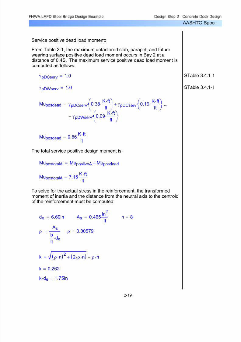
7/29/2019 LRFD steel design.pdf
http://slidepdf.com/reader/full/lrfd-steel-designpdf 79/646
k de⋅ 1.75in=
k 0.262=
k ρ n⋅( )22 ρ⋅ n⋅( )+ ρ n⋅−=
ρ 0.00579=ρ As
b
ft de⋅
=
n 8= As 0.465in
2
ft=de 6.69in=
To solve for the actual stress in the reinforcement, the transformedmoment of inertia and the distance from the neutral axis to the centroidof the reinforcement must be computed:
MupostotalA
7.15K ft⋅
ft=
MupostotalA MuposliveA Muposdead+=
The total service positive design moment is:
Muposdead 0.66K ft⋅
ft=
Muposdead γpDCserv 0.38K ft⋅
ft⋅⎛
⎝ ⎞ ⎠
⋅ γpDCserv 0.19K ft⋅
ft⋅⎛
⎝ ⎞ ⎠
⋅+
γpDWserv 0.09K ft⋅
ft
⋅⎛
⎝
⎞
⎠⋅+
...=
STable 3.4.1-1γpDWserv 1.0=
STable 3.4.1-1γpDCserv 1.0=
From Table 2-1, the maximum unfactored slab, parapet, and futurewearing surface positive dead load moment occurs in Bay 2 at a
distance of 0.4S. The maximum service positive dead load moment iscomputed as follows:
Service positive dead load moment:
2-19
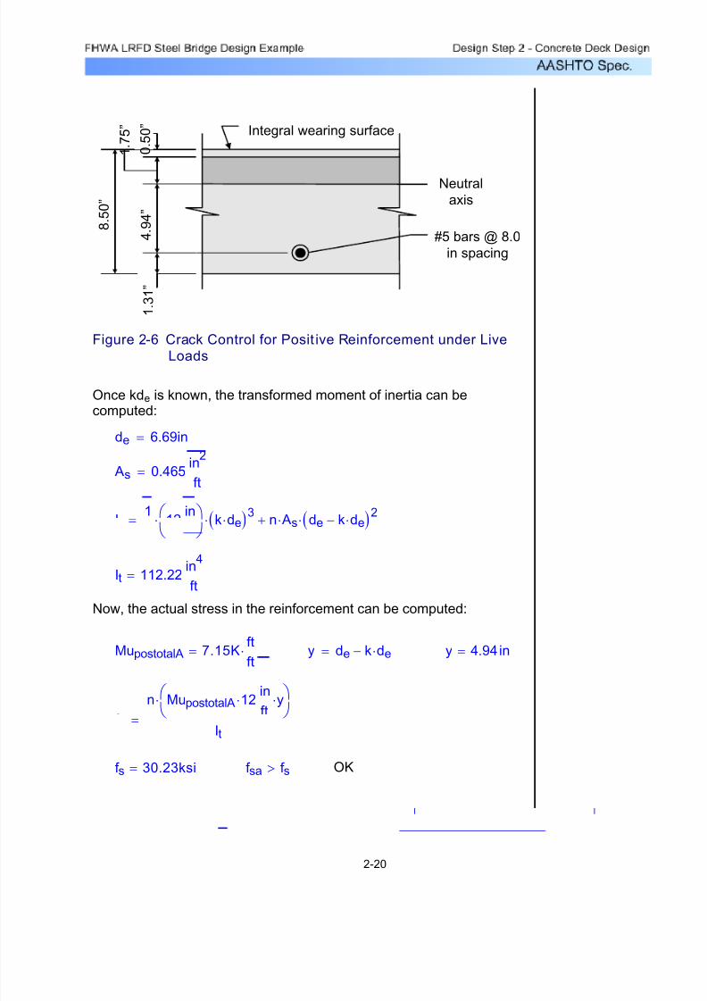
7/29/2019 LRFD steel design.pdf
http://slidepdf.com/reader/full/lrfd-steel-designpdf 80/646
1 . 7 5 ”
4 . 9 4 ”
Neutral
axis
Integral wearing surface
8 . 5 0 ”
0 . 5 0 ”
1 . 3 1 ”
#5 bars @ 8.0
in spacing
Figure 2-6 Crack Control for Posit ive Reinforcement under Live
Loads
Once kde is known, the transformed moment of inertia can becomputed:
de 6.69in=
As 0.465in
2
ft=
It
1
3 12
in
ft
⎛ ⎝
⎞ ⎠⋅ k de⋅( )
3
⋅ n As⋅ de k de⋅−( )
2
⋅+=
It 112.22in
4
ft=
Now, the actual stress in the reinforcement can be computed:
MupostotalA 7.15Kft
ft⋅= y de k de⋅−= y 4.94in=
f sn MupostotalA 12⋅
in
ft y⋅⎛ ⎝ ⎞ ⎠⋅
It=
f s 30.23ksi= f sa f s> OK
2-20
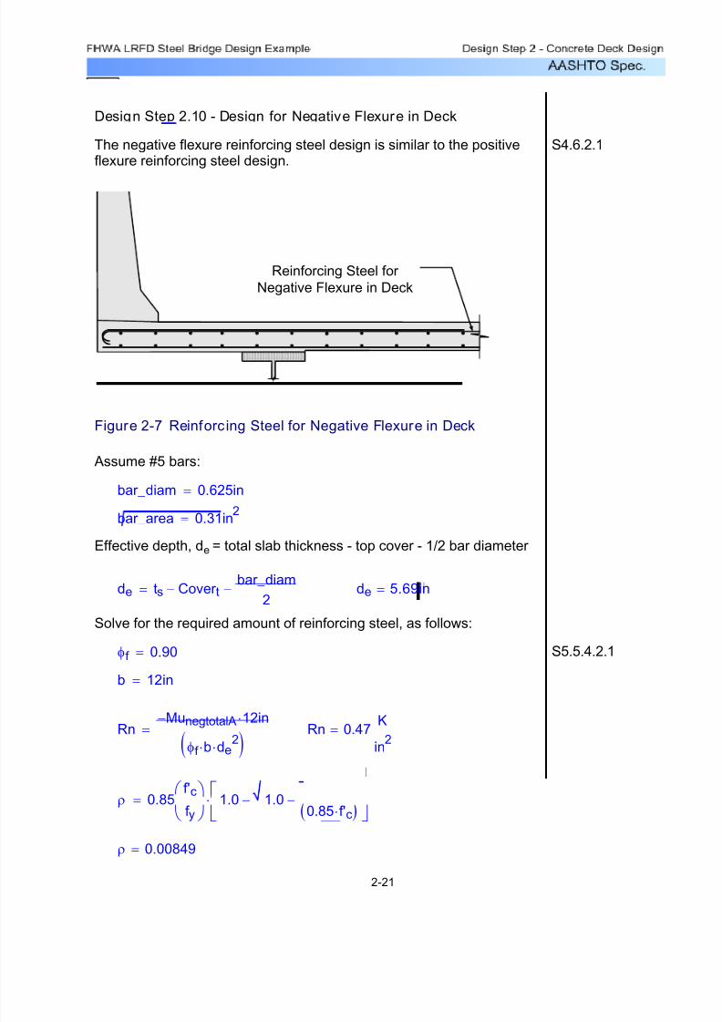
7/29/2019 LRFD steel design.pdf
http://slidepdf.com/reader/full/lrfd-steel-designpdf 81/646
ρ 0.00849=
ρ 0.85f'c
f y
⎛
⎝
⎞
⎠1.0 1.0
2 Rn⋅( )
0.85 f'c⋅( )−−⎡
⎣⎤⎦
⋅=
Rn 0.47K
in2
=RnMunegtotalA− 12⋅ in
φf b⋅ de2⋅( )
=
b 12in=
S5.5.4.2.1φf 0.90=
Solve for the required amount of reinforcing steel, as follows:
de 5.69in=de ts Cover t−bar_diam
2−=
Effective depth, de = total slab thickness - top cover - 1/2 bar diameter
bar_area 0.31in2=
bar_diam 0.625in=
Assume #5 bars:
Figure 2-7 Reinforc ing Steel for Negative Flexure in Deck
Reinforcing Steel for
Negative Flexure in Deck
S4.6.2.1The negative flexure reinforcing steel design is similar to the positiveflexure reinforcing steel design.
Design Step 2.10 - Design for Negative Flexure in Deck
2-21

7/29/2019 LRFD steel design.pdf
http://slidepdf.com/reader/full/lrfd-steel-designpdf 82/646
S5.7.3.4Note: clear cover is greater than 2.0 inches; therefore, use clear cover equals 2.0 inches.
Z 130K
in=
S5.7.3.4Similar to the positive flexure reinforcement, the control of cracking by
distribution of reinforcement must be checked.
Design Step 2.11 - Check for Negative Flexure Cracking under
Service Limit State
OK0.19 0.42≤
S5.7.3.3.1
c
de 0.42≤where
c
de 0.19=
S5.7.2.2c 1.07in=ca
β1
=
S5.7.2.2β1 0.85=
a 0.91 in=aT
0.85 f'c⋅ bar_space⋅=
T 18.60K=T bar_area f y⋅=
S5.7.3.3.1Once the bar size and spacing are known, the maximum reinforcement
limit must be checked.
bar_space 6.0in=Use #5 bars @
bar_area As
6.4in=Required bar spacing =
As 0.58in
2
ft= As ρ
b
ft⋅ de⋅=
2-22
7/29/2019 LRFD steel design.pdf
http://slidepdf.com/reader/full/lrfd-steel-designpdf 83/646
Munegdead γpDCservice 0.74−K ft⋅
ft⋅ 1.66
K ft⋅
ft−⎛
⎝ ⎞ ⎠
⋅
γpDWservice 0.06−K ft⋅
ft⋅⎛
⎝ ⎞ ⎠
⋅+
...=
STable 3.4.1-1γpDWservice 1.0=γpDCservice 1.0=
From Table 2-1, the maximum unfactored negative dead load moment
occurs in Bay 4 at a distance of 1.0S. The maximum service negativedead load moment is computed as follows:
Service negative dead load moment:
MunegliveA 6.07−K ft⋅
ft=
MunegliveA γLL 1 IM+( )⋅29.40− K ft⋅
wnegstripa⋅=
STable 3.4.1-1γLL 1.0=
From Table 2-2, the maximum unfactored negative live load moment is-29.40 K-ft, located at 0.0S in Bay 4 for two trucks. The maximumservice negative live load moment is:
Service negative live load moment:
f sa 32.47ksi=Use
0.6f y 36.00ksi=f sa 32.47ksi=
f sa 0.6 f y⋅≤wheref saZ
dc Ac⋅( )
1
3
=
Ac 27.75in2= Ac 2 dc( )⋅ bar_space⋅=
dc 2.31in=dc 2inbar_diam
2+=
2-23

7/29/2019 LRFD steel design.pdf
http://slidepdf.com/reader/full/lrfd-steel-designpdf 84/646
Munegdead 2.46−K ft⋅
ft=
The total service negative design moment is:
MunegtotalA MunegliveA Munegdead+=
MunegtotalA 8.53−K ft⋅
ft=
de 5.69in= As 0.62in
2
ft= n 8=
ρ
As
b
ftde⋅
= ρ 0.00908=
k ρ n⋅( )22 ρ⋅ n⋅( )+ ρ n⋅−=
k 0.315=
k de⋅ 1.79in=
Neutral
axis
2 . 8 1 ”
3 . 9 0 ”
1 . 7 9 ”
#5 bars @6.0 in spacing
8 . 5 0 ”
Figure 2-8 Crack Control for Negative Reinforcement under Live
Loads
2-24
7/29/2019 LRFD steel design.pdf
http://slidepdf.com/reader/full/lrfd-steel-designpdf 85/646
CA13.3.1
SA13.4.1Bridge deck overhangs must be designed to satisfy three differentdesign cases. In the first design case, the overhang must be designedfor horizontal (transverse and longitudinal) vehicular collision forces.For the second design case, the overhang must be designed to resistthe vertical collision force. Finally, for the third design case, theoverhang must be designed for dead and live loads. For DesignCases 1 and 2, the design forces are for the extreme event limit state.For Design Case 3, the design forces are for the strength limit state.
Also, the deck overhang region must be designed to have a resistancelarger than the actual resistance of the concrete parapet.
Design Step 2.12 - Design for Flexure in Deck Overhang
OKf sa f s>f s 32.44ksi=
f s
n MunegtotalA− 12⋅in
fty⋅⎛
⎝ ⎞ ⎠
⋅
It=
y 3.90in=y de k de⋅−=MunegtotalA 8.53− Kft
ft⋅=
Now, the actual stress in the reinforcement can be computed:
It 98.38in
4
ft=
It1
312
in
ft
⎛ ⎝
⎞ ⎠
⋅ k de⋅( )3⋅ n As⋅ de k de⋅−( )2⋅+=
As 0.62in
2
ft=
de 5.69in=
Once kde is known, the transformed moment of inertia can becomputed:
2-25
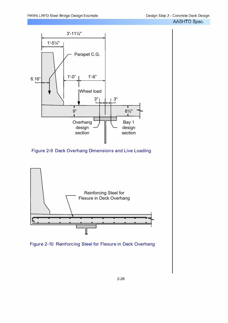
7/29/2019 LRFD steel design.pdf
http://slidepdf.com/reader/full/lrfd-steel-designpdf 86/646
1'-5¼"
Wheel load
3'-11¼"
3" 3"
8½"9”
6.16”1'-6”
Parapet C.G.
Overhang
design
section
Bay 1
design
section
1'-0”
Figure 2-9 Deck Overhang Dimensions and Live Loading
Reinforcing Steel for
Flexure in Deck Overhang
Figure 2-10 Reinforc ing Steel for Flexure in Deck Overhang
2-26

7/29/2019 LRFD steel design.pdf
http://slidepdf.com/reader/full/lrfd-steel-designpdf 87/646
Mutotal 28.97K ft⋅
ft=
Mutotal Mco MDCdeck+ MDCpar +=
MDCpar 0.61 K ft⋅ft
=
MDCpar γpDC Wpar ⋅ 1.4375ft6.16in
12in
ft
−⎛
⎝
⎞
⎠
⋅=
MDCdeck 0.15K ft⋅
ft=
MDCdeck
γpDC
9in
12in
ft
⎛
⎝
⎞
⎠
0.150kcf ( )⋅ 1.4375ft( )2⋅⎡
⎣
⎤
⎦2
⋅=
(see parapet properties)Mco 28.21Kft
ft⋅=
STable 3.4.1-2γpDC 1.25=
S1.3.2.1φext 1.0=
For the extreme event limit state:
The overhang must be designed for the vehicular collision plus deadload moment acting concurrently with the axial tension force fromvehicular collision.
Case 1A - Check at Inside Face of Parapet
The horizontal vehicular collision force must be checked at the insideface of the parapet, at the design section in the overhang, and at thedesign section in the first bay.
SA13.4.1Design Case 1 - Design Overhang for Horizontal Vehicular
Collision Force
2-27

7/29/2019 LRFD steel design.pdf
http://slidepdf.com/reader/full/lrfd-steel-designpdf 88/646
ftLc 12.84=
LcLt
2
Lt
2
⎛ ⎝
⎞ ⎠
28 H⋅ Mb Mw H⋅+( )⋅
Mc++=
Lc is then:
* Based on parapet properties not included in this design example.See Publication Number FHWA HI-95-017, Load and ResistanceFactor Design for Highway Bridges, Participant Notebook, Volume II(Version 3.01), for the method used to compute the parapet properties.
height of parapetftH 3.50=
flexural resistance of the wall about itsvertical axis
*K ft⋅Mw 18.52=
flexural resistance of the wall about an axisparallel to the longitudinal axis of the bridge
K ft⋅
ftMc 16.00= *
The axial tensile force is: SA13.4.2
TRw
Lc 2Hpar +
=
Before the axial tensile force can be calculated, the terms Lc and Rw need to be defined.
Lc is the critical wall length over which the yield line mechanism occurs: SA13.3.1
LcLt
2
Lt
2
⎛ ⎝
⎞ ⎠
28 H⋅ Mb Mw H⋅+( )⋅
Mc++=
Since the parapet is not designed in this design example, the variables
involved in this calculation are given below:
Lt 4= ft longitudinal length of distribution of impactforce Ft
SATable 13.2-1
Mb 0= K ft⋅ * additional flexural resistance of beam inaddition to Mw, if any, at top of wall
2-28
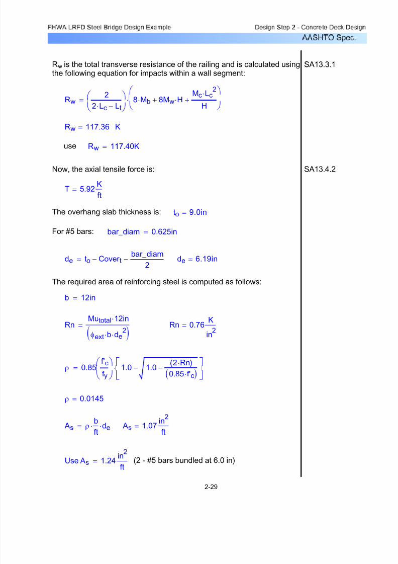
7/29/2019 LRFD steel design.pdf
http://slidepdf.com/reader/full/lrfd-steel-designpdf 89/646
(2 - #5 bars bundled at 6.0 in) As 1.24in
2
ft=Use
As 1.07in
2
ft= As ρ
b
ft⋅ de⋅=
ρ 0.0145=
ρ 0.85f'c
f y
⎛
⎝
⎞
⎠1.0 1.0
2 Rn⋅( )
0.85 f'c⋅( )−−⎡
⎣⎤⎦
⋅=
Rn 0.76K
in2
=RnMutotal 12⋅ in
φext b⋅ de2⋅( )
=
b 12in=
The required area of reinforcing steel is computed as follows:
de 6.19in=de to Cover t−bar_diam
2−=
bar_diam 0.625in=For #5 bars:
to 9.0in=The overhang slab thickness is:
T 5.92K
ft
=
SA13.4.2Now, the axial tensile force is:
Rw 117.40K=use
KRw 117.36=
Rw 22 Lc⋅ Lt−⎛ ⎝ ⎞ ⎠
8 Mb⋅ 8Mw H⋅+M
cL
c
2⋅
H+
⎛
⎝
⎞
⎠⋅=
SA13.3.1Rw is the total transverse resistance of the railing and is calculated usingthe following equation for impacts within a wall segment:
2-29
7/29/2019 LRFD steel design.pdf
http://slidepdf.com/reader/full/lrfd-steel-designpdf 90/646
The collision forces are distributed over a distance Lc for moment andLc + 2H for axial force. When the design section is moved to 1/4bf away from the girder centerline in the overhang, the distribution lengthwill increase. This example assumes a distribution length increasebased on a 30 degree angle from the face of the parapet.
Case 1B - Check at Design Section in Overhang
OK0.32 0.42≤
S5.7.3.3.1c
de0.42≤where
c
de0.32=
S5.7.2.2c 1.97 in=ca
β1
=
OKMr Mutotal≥
Mr 32.05K ft⋅
ft=Mr φext Mn⋅=
Mn 32.05K ft⋅
ft=Mn Ta dea
2−⎛ ⎝ ⎞ ⎠⋅ T
de
2
a
2−⎛ ⎝
⎞ ⎠⋅−=
a 1.68 in=aC
0.85 f'c⋅ b⋅=
C 68.48K=UseC 68.48K
ft=C Ta T−=
Ta 74.40
K
ft=Ta As f y⋅=
Once the required area of steel is known, the depth of the compressionblock must be checked:
2-30

7/29/2019 LRFD steel design.pdf
http://slidepdf.com/reader/full/lrfd-steel-designpdf 91/646
1'-5¼"
2'-3”
3'-11¼"
3"
8½"9”
Lc
= 12.84’
1.30’
30°
1.30’
30°
Figure 2-11 Assumed Distribut ion of Collision Moment
Load in the Overhang
2-31
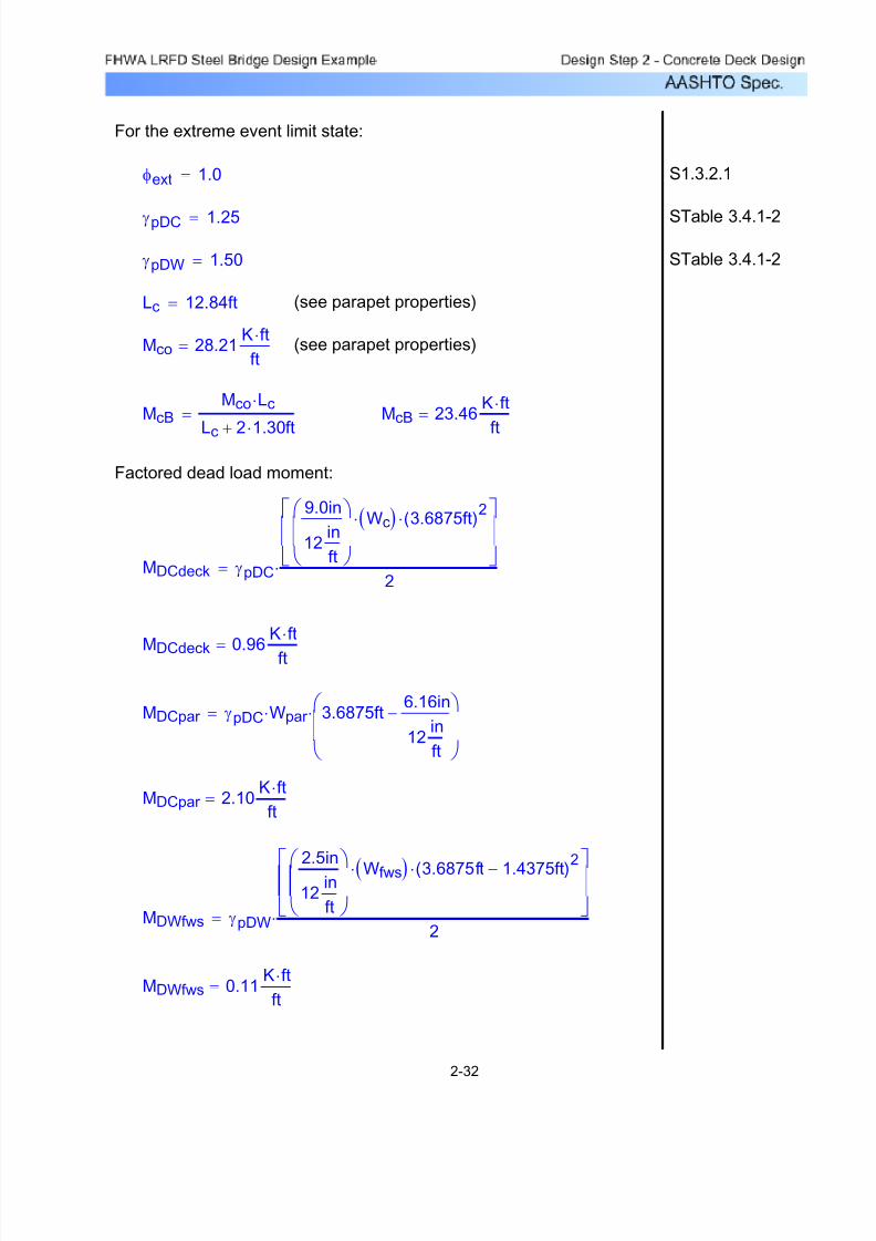
7/29/2019 LRFD steel design.pdf
http://slidepdf.com/reader/full/lrfd-steel-designpdf 92/646
MDWfws 0.11K ft⋅
ft=
MDWfws γpDW
2.5in
12in
ft
⎛ ⎝
⎞ ⎠
Wfws( )⋅ 3.6875ft 1.4375ft−( )2
⋅⎡⎣
⎤⎦
2⋅=
MDCpar 2.10K ft⋅
ft=
MDCpar γpDC Wpar ⋅ 3.6875ft6.16in
12in
ft
−⎛
⎝
⎞
⎠
⋅=
MDCdeck 0.96
K ft⋅
ft=
MDCdeck γpDC
9.0in
12in
ft
⎛
⎝
⎞
⎠
Wc( )⋅ 3.6875ft( )2⋅⎡
⎣
⎤
⎦2
⋅=
Factored dead load moment:
McB 23.46K ft⋅
ft
=McBMco Lc⋅
Lc 2 1.30⋅ ft+
=
(see parapet properties)Mco 28.21K ft⋅
ft=
(see parapet properties)Lc 12.84ft=
STable 3.4.1-2γpDW 1.50=
STable 3.4.1-2γpDC 1.25=
S1.3.2.1φext 1.0=
For the extreme event limit state:
2-32
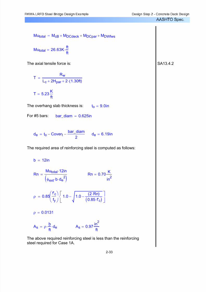
7/29/2019 LRFD steel design.pdf
http://slidepdf.com/reader/full/lrfd-steel-designpdf 93/646
The above required reinforcing steel is less than the reinforcingsteel required for Case 1A.
As 0.97in
2
ft= As ρ
b
ft⋅ de⋅=
ρ 0.0131=
ρ 0.85f'c
f y
⎛
⎝
⎞
⎠1.0 1.0
2 Rn⋅( )
0.85 f'c⋅( )−−
⎡
⎣
⎤
⎦⋅=
Rn 0.70K
in2
=RnMutotal 12⋅ in
φext b⋅ de2⋅( )
=
b 12in=
The required area of reinforcing steel is computed as follows:
de 6.19in=de to Cover t−bar_diam
2−=
bar_diam 0.625in=For #5 bars:
to 9.0in=The overhang slab thickness is:
T 5.23K
ft=
TRw
Lc 2Hpar + 2 1.30ft( )⋅+=
SA13.4.2The axial tensile force is:
Mutotal 26.63K
ft
ft⋅=
Mutotal McB MDCdeck+ MDCpar + MDWfws+=
2-33

7/29/2019 LRFD steel design.pdf
http://slidepdf.com/reader/full/lrfd-steel-designpdf 94/646
Case 1C - Check at Design Section in First Span
The total collision moment can be treated as shown in Figure 2-12.The moment ratio, M2/M1, can be calculated for the design strip. One
way to approximate this moment is to set it equal to the ratio of themoments produced by the parapet self-weight at the 0.0S points of thefirst and second bay. The collision moment per unit width can then bedetermined by using the increased distribution length based on the 30degree angle distribution (see Figure 2-11). The dead load momentsat this section can be obtained directly from Table 2-1.
M2
M1
Figure 2-12 Assumed Distribut ion of the Collision Moment
Across the Width of the Deck
Collision moment at exterior girder:
Mco 28.21−K ft⋅
ft= M1 Mco=
Parapet self-weight moment at Girder 1 (0.0S in Bay 1):
Par 1 1.66−K ft⋅
ft=
Parapet self-weight moment at Girder 2 (0.0S in Bay 2):
Par 2 0.47 K ft⋅ft
=
Collision moment at 1/4bf in Bay 1:
M2 M1Par 2
Par 1
⎛
⎝
⎞
⎠⋅= M2 7.99
K ft⋅
ft=
2-34

7/29/2019 LRFD steel design.pdf
http://slidepdf.com/reader/full/lrfd-steel-designpdf 95/646
MDWfws 0.09−K ft⋅
ft=
MDWfws γpDW 0.06−K ft⋅
ft
⎛ ⎝
⎞ ⎠
⋅=
MDCpar 2.08−K ft⋅
ft=
MDCpar γpDC 1.66−K ft⋅
ft
⎛
⎝
⎞
⎠
⋅=
MDCdeck 0.93− Kft
ft⋅=
MDCdeck γpDC 0.74−K ft⋅
ft
⎛ ⎝
⎞ ⎠
⋅=
Factored dead load moment (from Table 2-1):
McC 21.87−K ft⋅
ft=McC
McM2M1 Lc⋅
Lc 2 1.59ft( )⋅+=
McM2M1 27.28−K ft⋅
ft=
STable 3.4.1-2γpDW 1.50=
STable 3.4.1-2γpDC 1.25=
S1.3.2.1φext 1.0=
As in Case 1B, the 30 degree angle distribution will be used:
McM2M1 27.28−K ft⋅
ft=
McM2M1 Mco 0.25ftMco− M2+( )
9.75ft
⋅+=
By interpolation for a design section at 1/4bf in Bay 1, the totalcollision moment is:
2-35

7/29/2019 LRFD steel design.pdf
http://slidepdf.com/reader/full/lrfd-steel-designpdf 96/646
The above required reinforcing steel is less than the reinforcingsteel required for Case 1A.
As 1.01in
2
ft= As ρ
b
ft⋅ de⋅=
ρ 0.0148=
ρ 0.85f'c
f y
⎛
⎝
⎞
⎠1.0 1.0
2 Rn⋅( )
0.85 f'c⋅( )−−
⎡
⎣
⎤
⎦⋅=
Rn 0.77K
in2
=RnMutotal− 12⋅ in
φext b⋅ de2⋅( )
=
b 12in=
The required area of reinforcing steel is computed as follows:
de 5.69in=de ts Cover t−bar_diam
2−=
bar_diam 0.625in=For #5 bars:
ts 8.50in=Use a slab thickness equal to:
T 5.10K
ft=
TRw
Lc 2Hpar + 2 1.59ft( )⋅+=
SA13.4.2The axial tensile force is:
Mutotal 24.96−
K ft⋅
ft=
Mutotal McC MDCdeck+ MDCpar + MDWfws+=
2-36
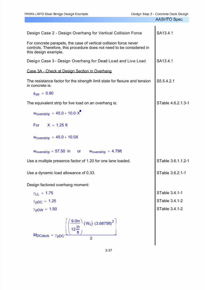
7/29/2019 LRFD steel design.pdf
http://slidepdf.com/reader/full/lrfd-steel-designpdf 97/646
MDCdeck γpDC
9.0in
12in
ft
⎛
⎝
⎞
⎠
Wc( )⋅ 3.6875ft( )2⋅⎡
⎣
⎤
⎦2
⋅=
STable 3.4.1-2γpDW 1.50=
STable 3.4.1-2γpDC
1.25=
STable 3.4.1-1γLL 1.75=
Design factored overhang moment:
STable 3.6.2.1-1Use a dynamic load allowance of 0.33.
STable 3.6.1.1.2-1Use a multiple presence factor of 1.20 for one lane loaded.
woverstrip 4.79ft=or inwoverstrip 57.50=
Design Case 2 - Design Overhang for Vertical Collision Force SA13.4.1
For concrete parapets, the case of vertical collision force never controls. Therefore, this procedure does not need to be considered in
this design example.
Design Case 3 - Design Overhang for Dead Load and Live Load SA13.4.1
Case 3A - Check at Design Section in Overhang
The resistance factor for the strength limit state for flexure and tensionin concrete is:
S5.5.4.2.1
φstr 0.90=
The equivalent strip for live load on an overhang is: STable 4.6.2.1.3-1
woverstrip 45.0 10.0 X⋅+=
For X 1.25= ft
woverstrip 45.0 10.0X+=
2-37

7/29/2019 LRFD steel design.pdf
http://slidepdf.com/reader/full/lrfd-steel-designpdf 98/646
Rn 0.43K
in2
=RnMutotal 12⋅ in
φstr b⋅ de2⋅( )
=
b 12in=
de 6.19in=
de to Cover t−bar_diam
2−=
bar_diam 0.625in=For #5 bars:
Calculate the required area of steel:
Mutotal 14.83K ft⋅
ft=
Mutotal MDCdeck MDCpar + MDWfws+ MLL+=
MLL 11.66K ft⋅
ft=
MLL γLL 1 IM+( )⋅ 1.20( )⋅16K
woverstrip
⎛ ⎝
⎞ ⎠
⋅ 1.25⋅ ft=
MDWfws 0.11K ft⋅
ft=
MDWfws γpDW Wfws⋅
2.5 in⋅
12in
ft⋅
⎛
⎝
⎞
⎠
3.6875 ft⋅ 1.4375 ft⋅−( )2⋅
2⋅=
MDCpar 2.10K ft⋅
ft=
MDCpar γpDC Wpar ⋅ 3.6875ft 6.16in
12in
ft
−⎛
⎝
⎞
⎠
⋅=
MDCdeck 0.96K ft⋅
ft=
2-38

7/29/2019 LRFD steel design.pdf
http://slidepdf.com/reader/full/lrfd-steel-designpdf 99/646
woverstrip 5.00ft=or inwoverstrip 60.00=
woverstrip 45.0 10.0X+=
ftX 1.50=For
woverstrip 45.0 10.0 X⋅+=
STable 3.4.1-2γpDW 1.50=
STable 3.4.1-2γpDC 1.25=
STable 3.4.1-1γLL
1.75=
Design factored moment:
The dead and live load moments are taken from Tables 2-1 and 2-2.The maximum negative live load moment occurs in Bay 4. Since thenegative live load moment is produced by a load on the overhang,compute the equivalent strip based on a moment arm to the centerlineof girder.
ts 8.50in=Use a slab thickness equal to:
Case 3B - Check at Design Section in First Span
The above required reinforcing steel is less than the reinforcingsteel required for Cases 1A, 1B, and 1C.
As 0.57in
2
ft= As ρ
b
ft⋅ de⋅=
ρ 0.00770=
ρ 0.85f'c
f y
⎛
⎝
⎞
⎠1.0 1.0
2 Rn⋅( )
0.85 f'c⋅( )−−⎡
⎣
⎤
⎦⋅=
2-39

7/29/2019 LRFD steel design.pdf
http://slidepdf.com/reader/full/lrfd-steel-designpdf 100/646
b 12in=
de 5.69in=
de ts Cover t−bar_diam
2−=
bar_diam 0.625in=For #5 bars:
Calculate the required area of steel:
Mutotal 16.78−K ft⋅
ft=
Mutotal MDCdeck MDCpar + MDWfws+ MLL+=
MLL 13.69−K ft⋅
ft=
MLL γLL 1 IM+( )⋅29.40− K ft⋅( )
woverstrip⋅=
MDWfws 0.09−K ft⋅
ft=
MDWfws γpDW 0.06−
K ft⋅
ft
⎛ ⎝
⎞ ⎠⋅=
MDCpar 2.08−K ft⋅
ft=
MDCpar γpDC 1.66−K ft⋅
ft
⎛ ⎝
⎞ ⎠
⋅=
MDCdeck 0.93−K ft⋅
ft=
MDCdeck γpDC 0.74−K ft⋅
ft
⎛ ⎝
⎞ ⎠
⋅=
2-40

7/29/2019 LRFD steel design.pdf
http://slidepdf.com/reader/full/lrfd-steel-designpdf 101/646
Since the area of reinforcing steel required in the overhang is greater than the area of reinforcing steel required in the negative momentregions, reinforcement must be added in the overhang area to satisfythe design requirements.
0.62in
2
ft1.24
in2
ft<
Asneg
0.62in
2
ft=
Asnegbar_area
ft
12in
6in
⎛ ⎝
⎞ ⎠
⋅=
bar_area 0.31in2=
bar_diam 0.625in=#5 bars at 6.0 inches:
The negative flexure reinforcement provided from the design in Steps
2.10 and 2.11 is:
As 1.24in
2
ft=Case 1A controls with:
The required area of reinforcing steel in the overhang is the largest of that required for Cases 1A, 1B, 1C, 3A, and 3B.
The above required reinforcing steel is less than the reinforcing steelrequired for Cases 1A, 1B, and 1C.
As 0.72in
2
ft= As ρ
b
ft⋅ de⋅=
ρ 0.0106=
ρ 0.85f'c
f y
⎛
⎝
⎞
⎠1.0 1.0
2 Rn⋅( )
0.85 f'c⋅( )−−
⎡
⎣
⎤
⎦⋅=
Rn 0.58K
in2
=RnMutotal− 12⋅ in
φstr b⋅ de2⋅( )
=
2-41

7/29/2019 LRFD steel design.pdf
http://slidepdf.com/reader/full/lrfd-steel-designpdf 102/646
Cracking in the overhang must be checked for the controlling serviceload (similar to Design Steps 2.9 and 2.11). In most deck overhangdesign cases, cracking does not control. Therefore, the computationsfor the cracking check are not shown in this deck overhang designexample.
Design Step 2.13 - Check for Cracking in Overhang under ServiceLimit State
OK0.38 0.42≤
S5.7.3.3.1c
de0.42≤where
c
demin0.38=
S5.7.2.2c 2.15 in=ca
β1
=
a 1.82in=aT
0.85 f'c⋅ b⋅=
T 74.40K=UseT 74.40K
ft=T As f y⋅=
demin 5.69in=
demin ts Cover t− bar_diam2
−=
Once the required area of reinforcing steel is known, the depth of thecompression block must be checked. The ratio of c/de is more criticalat the minimum deck thickness, so c/de will be checked in Bay 1 wherethe deck thickness is 8.5 inches.
As 1.24in
2
ft=
As 2 0.31in
2
ft⋅
⎛
⎝
⎞
⎠⋅
12in
6in
⎛
⎝
⎞
⎠⋅=The new area of reinforcing steel is now:
Bundle one #5 bar to each negative flexure reinforcing bar in theoverhang area.
2-42
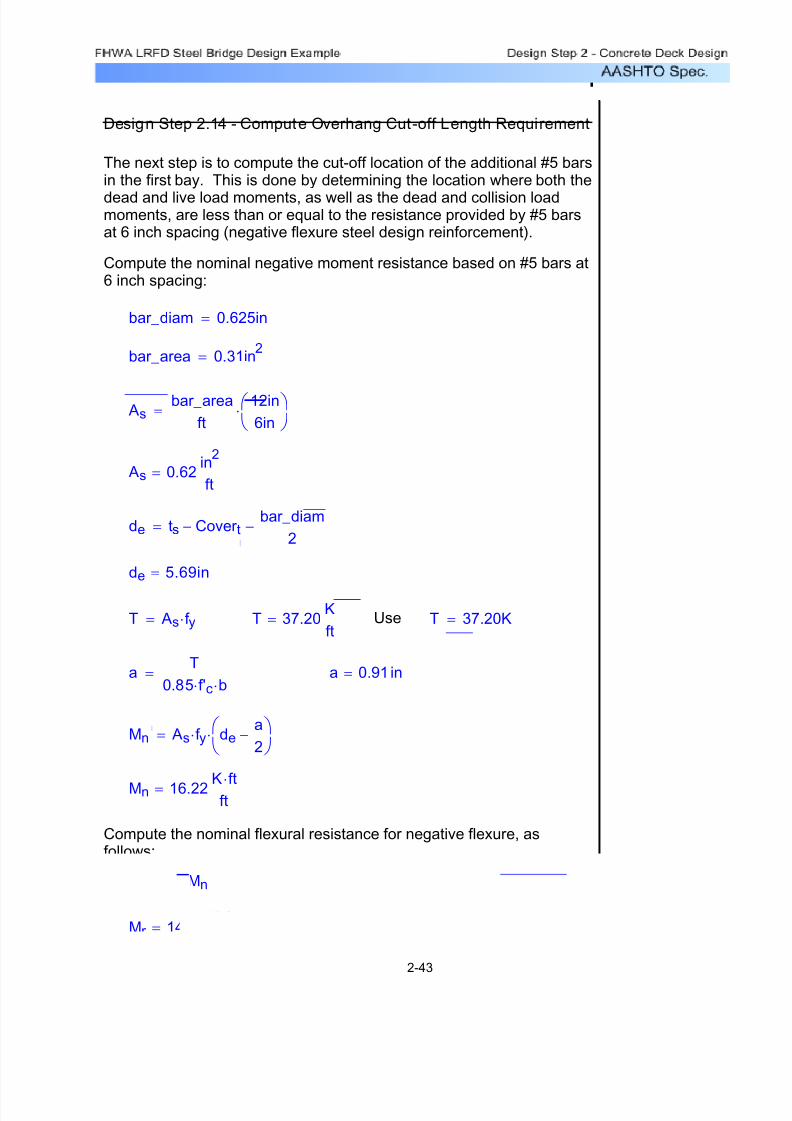
7/29/2019 LRFD steel design.pdf
http://slidepdf.com/reader/full/lrfd-steel-designpdf 103/646
Mr 14.60K ft⋅
ft=
Mr φf Mn⋅=
Compute the nominal flexural resistance for negative flexure, asfollows:
Mn 16.22 K ft⋅ft=
Mn As f y⋅ dea
2−⎛
⎝ ⎞ ⎠
⋅=
a 0.91 in=aT
0.85 f'c⋅ b⋅=
T 37.20K=UseT 37.20K
ft=T As f y⋅=
de 5.69in=
de ts Cover t−bar_diam
2−=
As 0.62in
2
ft=
Asbar_area
ft
12in
6in
⎛ ⎝
⎞ ⎠
⋅=
bar_area 0.31in2=
bar_diam 0.625in=
Compute the nominal negative moment resistance based on #5 bars at6 inch spacing:
The next step is to compute the cut-off location of the additional #5 barsin the first bay. This is done by determining the location where both the
dead and live load moments, as well as the dead and collision loadmoments, are less than or equal to the resistance provided by #5 barsat 6 inch spacing (negative flexure steel design reinforcement).
Design Step 2.14 - Compute Overhang Cut-off Length Requirement
2-43
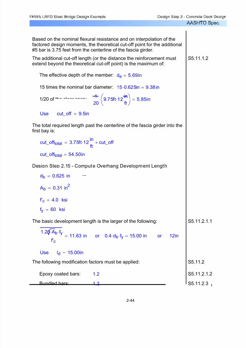
7/29/2019 LRFD steel design.pdf
http://slidepdf.com/reader/full/lrfd-steel-designpdf 104/646
ksi
f y 60= ksi
The basic development length is the larger of the following: S5.11.2.1.1
1.25 Ab⋅ f y⋅
f'c11.63= in or 0.4 db⋅ f y⋅ 15.00= in or 12in
Use ld 15.00in=
The following modification factors must be applied: S5.11.2
Epoxy coated bars: 1.2 S5.11.2.1.2
Bundled bars: 1.2 S5.11.2.3
Based on the nominal flexural resistance and on interpolation of thefactored design moments, the theoretical cut-off point for the additional#5 bar is 3.75 feet from the centerline of the fascia girder.
The additional cut-off length (or the distance the reinforcement mustextend beyond the theoretical cut-off point) is the maximum of:
S5.11.1.2
The effective depth of the member: de 5.69in=
15 times the nominal bar diameter: 15 0.625⋅ in 9.38in=
1/20 of the clear span:1
209.75ft 12⋅
in
ft
⎛ ⎝
⎞ ⎠
⋅ 5.85in=
Use cut_off 9.5in=
The total required length past the centerline of the fascia girder into thefirst bay is:
cut_off total 3.75ft 12⋅in
ftcut_off +=
cut_off total 54.50in=
Design Step 2.15 - Compute Overhang Development Length
db 0.625= in
Ab 0.31= in2
f'c 4.0=
2-44

7/29/2019 LRFD steel design.pdf
http://slidepdf.com/reader/full/lrfd-steel-designpdf 105/646
Spacing > 6 inches with more than 3 inchesof clear cover in direction of spacing: 0.8 S5.11.2.1.3
ld 15.00in 1.2( )⋅ 1.2( )⋅ 0.8( )⋅=
ld 17.28in= Use ld 18.00in=
The required length past the centerline of the fascia girder is:
3.0in ld+ 21.00in=
21.00in 54.50in< provided
3"
Bay 1
design
section
54½"
45" 9½" Cut-off length
21"
18.0" Development length
#5 bars @ 6 in
(bundled bars)
Figure 2-13 Length of Overhang Negative MomentReinforcement
2-45
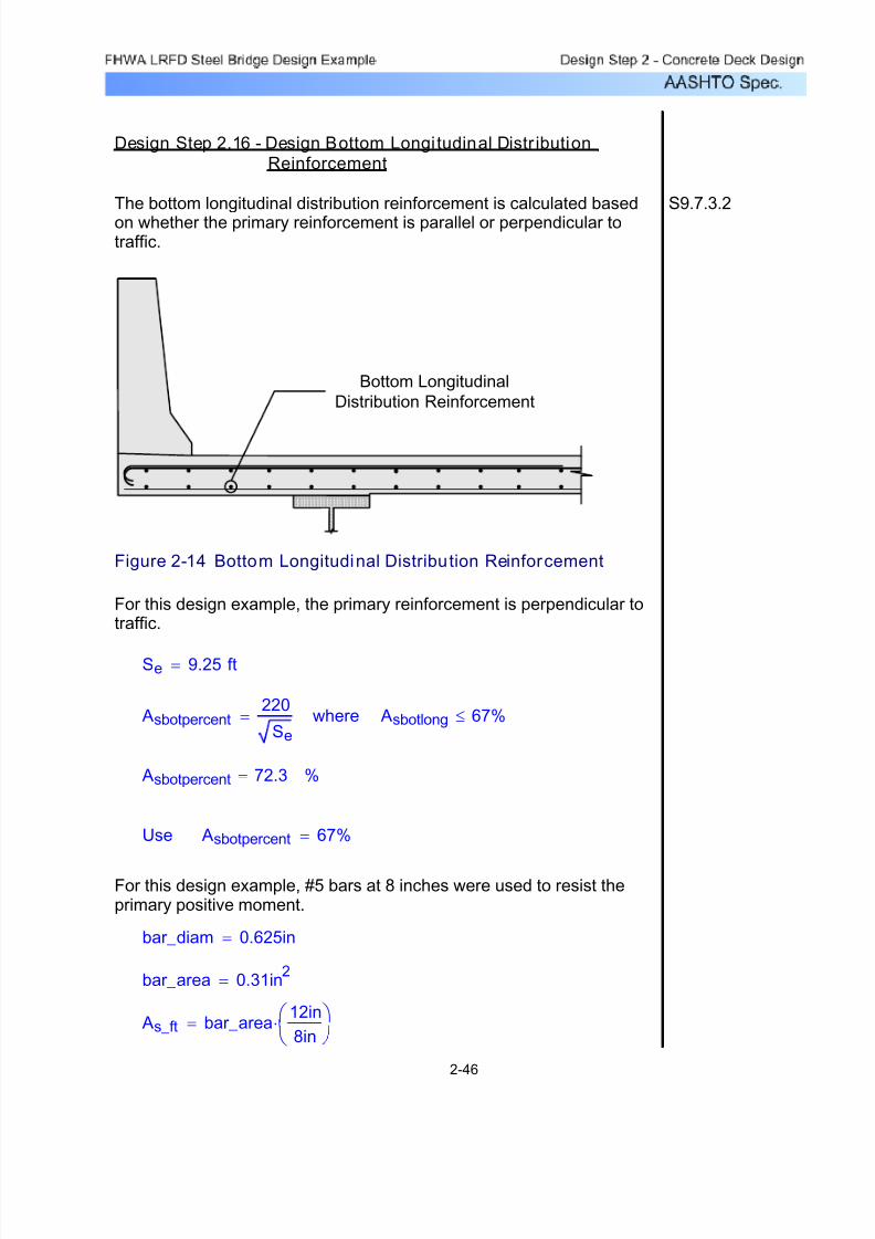
7/29/2019 LRFD steel design.pdf
http://slidepdf.com/reader/full/lrfd-steel-designpdf 106/646
As_ft bar_area12in
8in
⎛ ⎝
⎞⋅=
bar_area 0.31in2=
bar_diam 0.625in=
For this design example, #5 bars at 8 inches were used to resist theprimary positive moment.
Asbotpercent 67%=Use
% Asbotpercent 72.3=
Asbotlong 67%≤where Asbotpercent220
Se
=
ftSe 9.25=
For this design example, the primary reinforcement is perpendicular totraffic.
Figure 2-14 Bottom Longitudinal Distribution Reinforcement
Bottom Longitudinal
Distribution Reinforcement
S9.7.3.2The bottom longitudinal distribution reinforcement is calculated based
on whether the primary reinforcement is parallel or perpendicular totraffic.
Design Step 2.16 - Design Bottom Longi tudinal Distr ibution
Reinforcement
2-46

7/29/2019 LRFD steel design.pdf
http://slidepdf.com/reader/full/lrfd-steel-designpdf 107/646
As_ft 0.465in
2
ft=
Asbotlong
Asbotpercent
As_ft
⋅=
Asbotlong 0.31in
2
ft=
Calculate the required spacing using #5 bars:
spacingbar_area
Asbotlong=
spacing 1.00 ft= or spacing 11.94 in=
Use spacing 10in=
Use #5 bars at 10 inch spacing for the bottom longitudinalreinforcement.
Design Step 2.17 - Design Top Longitudinal Distr ibution
Reinforcement
Top Longitudinal
Distribution Reinforcement
Figure 2-15 Top Longitudinal Distr ibution Reinforcement
2-47
7/29/2019 LRFD steel design.pdf
http://slidepdf.com/reader/full/lrfd-steel-designpdf 108/646
Use #4 bars at 10 inch spacing for the top longitudinal temperature andshrinkage reinforcement.
OK 0.24in
2
ft0.10
in2
ft>
Asact 0.24in2
ft= Asact 0.20
in2
ft⋅
12in
10in⎛ ⎝
⎞ ⎠
⋅=
Check #4 bars at 10 inch spacing:
Asreq 0.10in
2
ft= Asreq
0.19in
2
ft⋅
2=
The amount of steel required for the top longitudinal reinforcement is:
When using the above equation, the calculated area of reinforcingsteel must be equally distributed on both concrete faces. In addition,
the maximum spacing of the temperature and shrinkage reinforcementmust be the smaller of 3.0 times the deck thickness or 18.0 inches.
0.11 Ag
f y0.19
in2
ft=
Ag 102.00in
2
ft= Ag 8.5in 12.0
in
ft
⎛ ⎝
⎞ ⎠
⋅=
As 0.11
Ag
f y≥
S5.10.8.2The top longitudinal temperature and shrinkage reinforcement mustsatisfy:
2-48
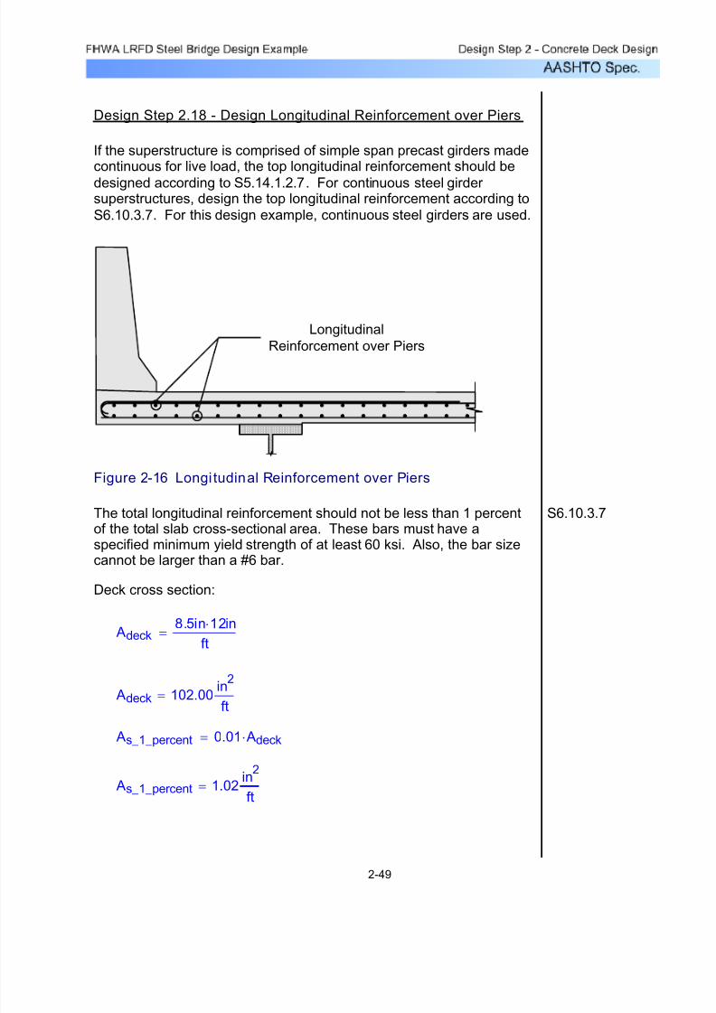
7/29/2019 LRFD steel design.pdf
http://slidepdf.com/reader/full/lrfd-steel-designpdf 109/646
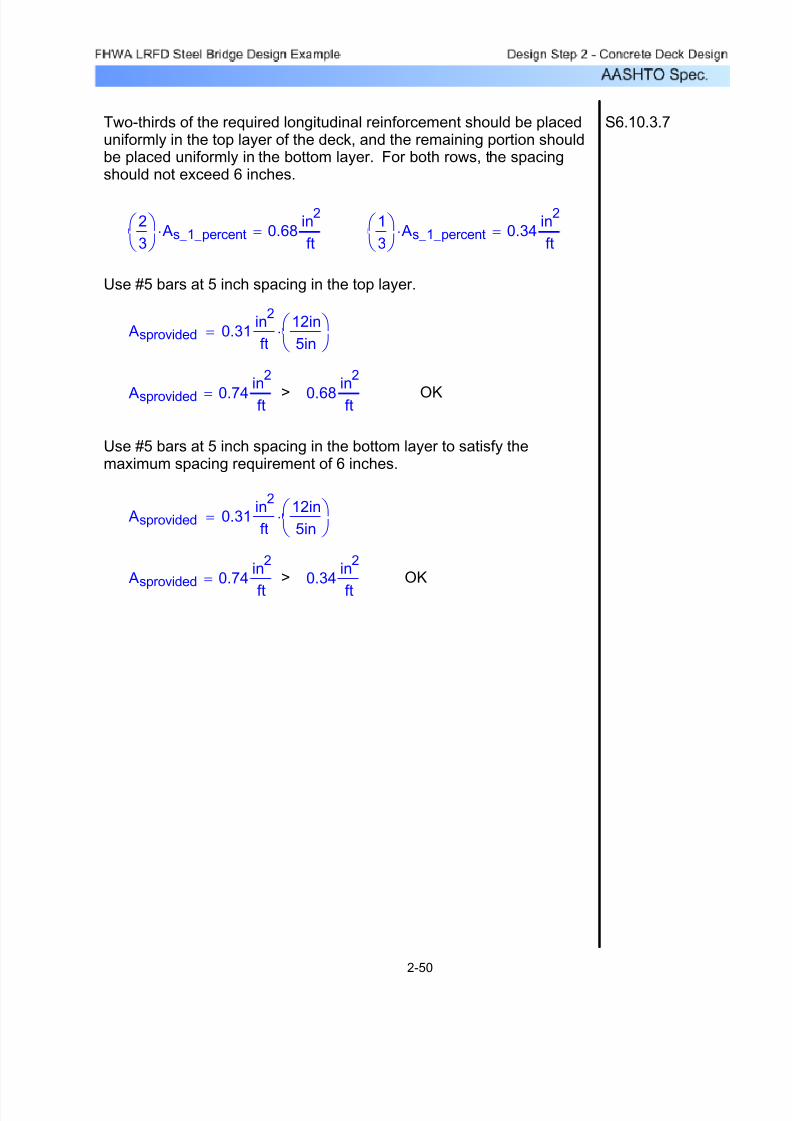
7/29/2019 LRFD steel design.pdf
http://slidepdf.com/reader/full/lrfd-steel-designpdf 110/646
OK 0.34in
2
ft> Asprovided 0.74
in2
ft=
Asprovided 0.31in
2
ft
12in
5in
⎛ ⎝
⎞ ⎠
⋅=
Use #5 bars at 5 inch spacing in the bottom layer to satisfy themaximum spacing requirement of 6 inches.
OK 0.68in
2
ft> Asprovided 0.74in
2
ft=
Asprovided 0.31in
2
ft
12in
5in
⎛ ⎝
⎞ ⎠
⋅=
Use #5 bars at 5 inch spacing in the top layer.
1
3
⎛ ⎝
⎞ ⎠
As_1_percent⋅ 0.34in
2
ft=
2
3
⎛ ⎝
⎞ ⎠
As_1_percent⋅ 0.68in
2
ft=
S6.10.3.7Two-thirds of the required longitudinal reinforcement should be placeduniformly in the top layer of the deck, and the remaining portion shouldbe placed uniformly in the bottom layer. For both rows, the spacingshould not exceed 6 inches.
2-50

7/29/2019 LRFD steel design.pdf
http://slidepdf.com/reader/full/lrfd-steel-designpdf 111/646
Design Step 2.19 - Draw Schematic of Final ConcreteDeck Design
54½"
#5 @ 8 in
2½" Cl.
1" Cl.
8½"
#5 @ 10 in
#5 @ 6 in#5 @ 6 in
(bundled bar)
9”
#4 @ 10 in
Figure 2-17 Superstructure Posit ive Moment Deck Reinforcement
54½"
#5 @ 8 in
2½" Cl.
1" Cl.
8½"
#5 @ 5 in
#5 @ 6 in#5 @ 6 in
(bundled bar)
#5 @ 5 in
9”
Figure 2-18 Superstructure Negative Moment Deck Reinforcement
2-51

7/29/2019 LRFD steel design.pdf
http://slidepdf.com/reader/full/lrfd-steel-designpdf 112/646
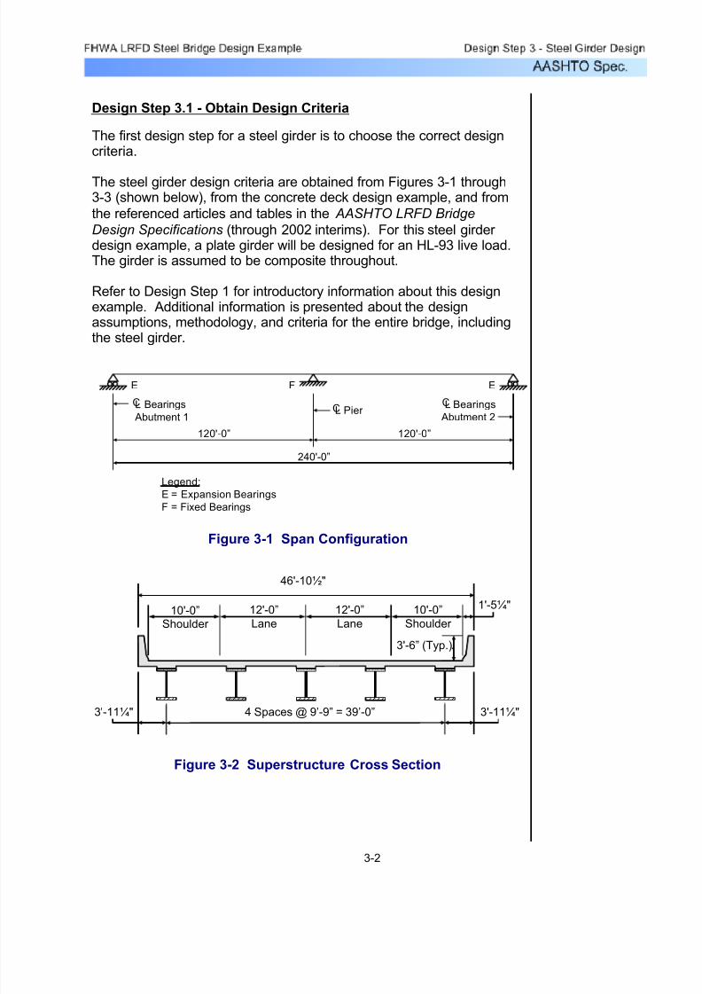
7/29/2019 LRFD steel design.pdf
http://slidepdf.com/reader/full/lrfd-steel-designpdf 113/646
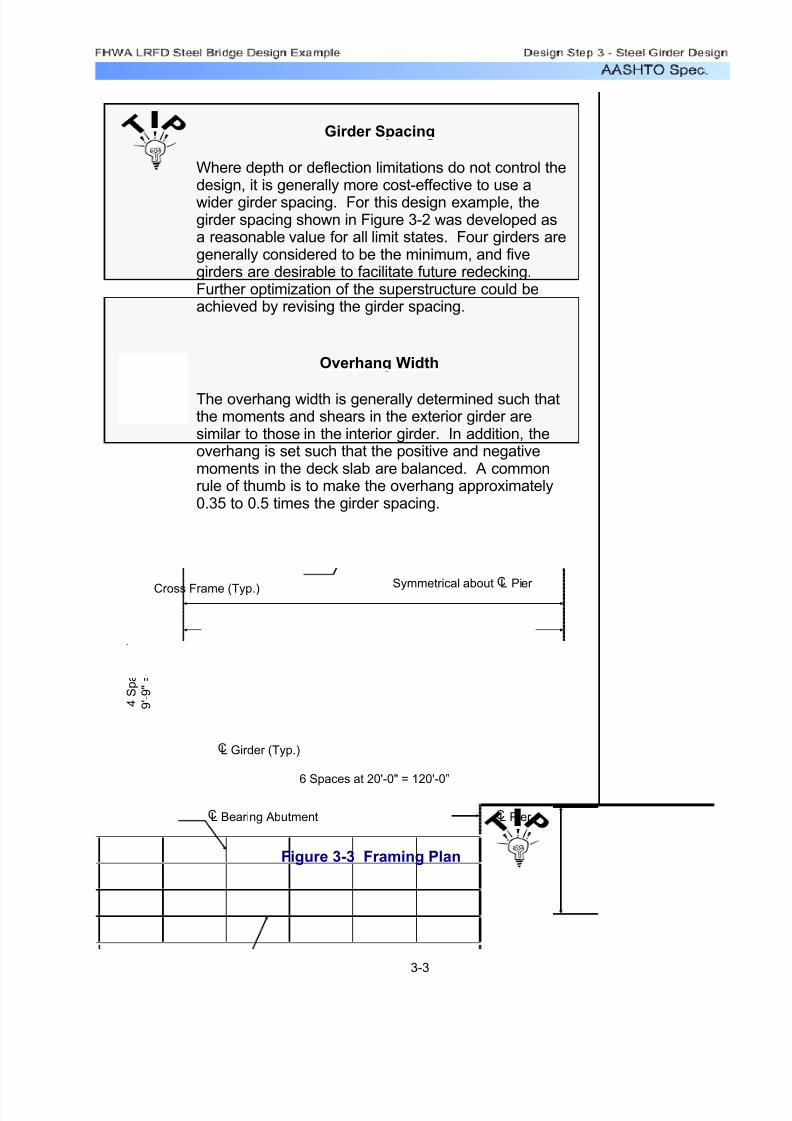
7/29/2019 LRFD steel design.pdf
http://slidepdf.com/reader/full/lrfd-steel-designpdf 114/646
Girder Spacing
Where depth or deflection limitations do not control thedesign, it is generally more cost-effective to use awider girder spacing. For this design example, thegirder spacing shown in Figure 3-2 was developed asa reasonable value for all limit states. Four girders aregenerally considered to be the minimum, and fivegirders are desirable to facilitate future redecking.Further optimization of the superstructure could beachieved by revising the girder spacing.
Overhang Width
The overhang width is generally determined such thatthe moments and shears in the exterior girder aresimilar to those in the interior girder. In addition, theoverhang is set such that the positive and negativemoments in the deck slab are balanced. A commonrule of thumb is to make the overhang approximately0.35 to 0.5 times the girder spacing.
4 S p a c e s a t
9 ' - 9 " = 3 9 ' - 0 "
L Bearing Abutment L Pier C C
6 Spaces at 20'-0" = 120'-0”
Cross Frame (Typ.)
L Girder (Typ.)C
Symmetrical about L Pier C
Figure 3-3 Framing Plan
3-3

7/29/2019 LRFD steel design.pdf
http://slidepdf.com/reader/full/lrfd-steel-designpdf 115/646
S 9.75ft=
Deck overhang: Soverhang 3.9375ft=
Cross-frame spacing: Lb 20ft= S6.7.4
Web yield strength: Fyw 50ksi= STable 6.4.1-1
Flange yield strength: Fyf 50ksi= STable 6.4.1-1
Concrete 28-daycompressive strength:
S5.4.2.1 &
STable C5.4.2.1-1f'c 4.0ksi=
Reinforcementstrength: f y 60ksi= S5.4.3 & S6.10.3.7
Cross-frame Spacing
A common rule of thumb, based on previous editionsof the AASHTO Specifications, is to use a maximumcross-frame spacing of 25 feet.
For this design example, a cross-frame spacing of 20feet is used because it facilitates a reduction in therequired flange thicknesses in the girder section at thepier.
This spacing also affects constructibility checks for stability before the deck is cured. Currently,stay-in-place forms should not be considered toprovide adequate bracing to the top flange.
The following units are defined for use in this design example:
K 1000lb= kcf K
ft3
= ksf K
ft2
= ksiK
in2
=
Design criteria:
Number of spans: Nspans 2=
Span length: Lspan 120ft=
Skew angle: Skew 0deg=
Number of girders: Ngirders 5=
Girder spacing:
3-4
7/29/2019 LRFD steel design.pdf
http://slidepdf.com/reader/full/lrfd-steel-designpdf 116/646
Stay-in-place deck formweight: Wdeckforms 0.015ksf =
Parapet weight (each): Wpar 0.53K
ft=
Future wearing surface: Wfws 0.140kcf = STable 3.5.1-1
Future wearingsurface thickness: tfws 2.5in=
Deck width: wdeck 46.875ft=Roadway width: wroadway 44.0ft=
Haunch depth (from topof web): dhaunch 3.5in=
Average Daily TruckTraffic (Single-Lane):
ADTTSL 3000=
For this design example, transverse stiffeners will be designed in
Step 3.12. In addition, a bolted field splice will be designed in Step4, shear connectors will be designed in Step 5.1, bearing stiffenerswill be designed in Step 5.2, welded connections will be designed inStep 5.3, cross-frames are described in Step 5.4, and anelastomeric bearing will be designed in Step 6. Longitudinalstiffeners will not be used, and a deck pouring sequence will not beconsidered in this design example.
Design criteria (continued):
Total deck thickness: tdeck 8.5in=
Effective deck thickness: teffdeck 8.0in=Total overhang thickness: toverhang 9.0in=
Effective overhangthickness: teffoverhang 8.5in=
Steel density: Ws 0.490kcf = STable 3.5.1-1
Concrete density: Wc 0.150kcf = STable 3.5.1-1
Additional miscellaneousdead load (per girder): Wmisc 0.015
K
ft
=
3-5

7/29/2019 LRFD steel design.pdf
http://slidepdf.com/reader/full/lrfd-steel-designpdf 117/646

7/29/2019 LRFD steel design.pdf
http://slidepdf.com/reader/full/lrfd-steel-designpdf 118/646
Multiple Presence Factors
Multiple presence factors are described in S3.6.1.1.2 .
They are already included in the computation of liveload distribution factors, as presented in S4.6.2.2 . Anexception, however, is that they must be included whenthe live load distribution factor for an exterior girder iscomputed assuming that the cross section deflectsand rotates as a rigid cross section, as presented inS4.6.2.2.2d .
Since S3.6.1.1.2 states that the effects of the multiplepresence factor are not to be applied to the fatiguelimit state, all emperically determined distribution
factors for one-lane loaded that are applied to thesingle fatigue truck must be divided by 1.20 (that is,the multiple presence factor for one lane loaded). Inaddition, for distribution factors computed using the
lever rule or based on S4.6.2.2.2d , the 1.20 factor should not be included when computing the distributionfactor for one-lane loaded for the fatigue limit state. Itshould also be noted that the multiple presence factor still applies to the distribution factors for one-laneloaded for strength limit states.
Dynamic load allowance: STable 3.6.2.1-1
Fatigue and Fracture
Limit State15%
All Other Limit States 33%
Dynamic Load AllowanceDynamic Load
Allowance, IMLimit State
Table 3-3 Dynamic Load Allowance
Dynamic load allowance is the same as impact. The term"impact" was used in previous editions of the AASHTOSpecifications. However, the term "dynamic load allowance" is
used in the AASHTO LRFD Bridge Design Specifications.
3-7
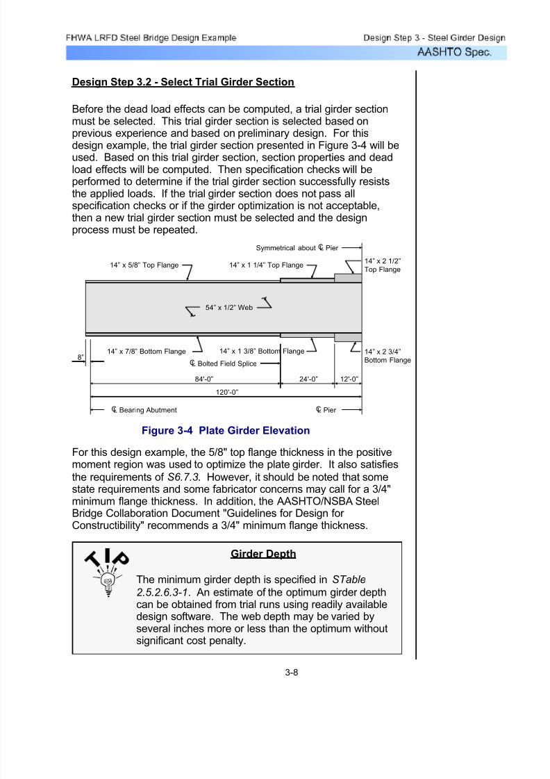
7/29/2019 LRFD steel design.pdf
http://slidepdf.com/reader/full/lrfd-steel-designpdf 119/646
Design Step 3.2 - Select Trial Girder Section
Before the dead load effects can be computed, a trial girder sectionmust be selected. This trial girder section is selected based on
previous experience and based on preliminary design. For thisdesign example, the trial girder section presented in Figure 3-4 will beused. Based on this trial girder section, section properties and deadload effects will be computed. Then specification checks will beperformed to determine if the trial girder section successfully resiststhe applied loads. If the trial girder section does not pass allspecification checks or if the girder optimization is not acceptable,then a new trial girder section must be selected and the designprocess must be repeated.
84'-0” 12'-0”
120'-0”
14” x 7/8” Bottom Flange
14” x 1 1/4” Top Flange
14” x 2 3/4”
Bottom Flange
14” x 2 1/2”
Top Flange
L Bearing Abutment L Pier
Symmetrical about L Pier
L Bolted Field Splice
54” x 1/2” Web
C
C
C C
8”
24'-0”
14” x 1 3/8” Bottom Flange
14” x 5/8” Top Flange
Figure 3-4 Plate Girder Elevation
For this design example, the 5/8" top flange thickness in the positivemoment region was used to optimize the plate girder. It also satisfies
the requirements of S6.7.3. However, it should be noted that somestate requirements and some fabricator concerns may call for a 3/4"minimum flange thickness. In addition, the AASHTO/NSBA SteelBridge Collaboration Document "Guidelines for Design for Constructibility" recommends a 3/4" minimum flange thickness.
Girder Depth
The minimum girder depth is specified in STable
2.5.2.6.3-1. An estimate of the optimum girder depthcan be obtained from trial runs using readily availabledesign software. The web depth may be varied byseveral inches more or less than the optimum withoutsignificant cost penalty.
3-8

7/29/2019 LRFD steel design.pdf
http://slidepdf.com/reader/full/lrfd-steel-designpdf 120/646
Web Thickness
A "nominally stiffened" web (approximately 1/16 inch
thinner than "unstiffened") will generally provide theleast cost alternative or very close to it. However, for web depths of approximately 50 inches or less,unstiffened webs may be more economical.
Plate Transitions
A common rule of thumb is to use no more than threeplates (two shop splices) in the top or bottom flange of field sections up to 130 feet long. In some cases, a
single flange plate size can be carried through the fulllength of the field section.
Flange Widths
Flange widths should remain constant within fieldsections. The use of constant flange widths simplifiesconstruction of the deck. The unsupported length incompression of the shipping piece divided by theminimum width of the compression flange in that piece
should be less than approximately 85.
Flange Plate Transitions
It is good design practice to reduce the flangecross-sectional area by no more than approximatelyone-half of the area of the heavier flange plate. Thisreduces the build-up of stress at the transition.
The above tips are presented to help bridge designers in developingan economical steel girder for most steel girder designs. Other design tips are available in various publications from the AmericanInstitute of Steel Construction (AISC) and from steel fabricators.
3-9

7/29/2019 LRFD steel design.pdf
http://slidepdf.com/reader/full/lrfd-steel-designpdf 121/646
Design Step 3.3 - Compute Section Properties
Since the superstructure is composite, several sets of sectionproperties must be computed. The initial dead loads (or thenoncomposite dead loads) are applied to the girder-only section.The superimposed dead loads are applied to the composite sectionbased on a modular ratio of 3n or n, whichever gives the higher stresses.
S6.10.3.1
S6.10.3.1.1b
Modular Ratio
As specified in S6.10.3.1.1b, for permanent loadsassumed to be applied to the long-term compositesection, the slab area shall be transformed by using amodular ratio of 3n or n, whichever gives the higher stresses.
Using a modular ratio of 3n for the superimposeddead loads always gives higher stresses in the steelsection. Using a modular ratio of n typically giveshigher stresses in the concrete deck, except in themoment reversal regions where the selection of 3n vs.n can become an issue in determining the maximumstress in the deck.
The live loads are applied to the composite section based on a
modular ratio of n.
For girders with shear connectors provided throughout their entirelength and with slab reinforcement satisfying the provisions of
S6.10.3.7 , stresses due to loads applied to the composite section for service and fatigue limit states may be computed using the compositesection assuming the concrete slab to be fully effective for bothpositive and negative flexure.
Therefore, for this design example, the concrete slab will be assumedto be fully effective for both positive and negative flexure for service
and fatigue limit states.
For this design example, the interior girder controls. In general, boththe exterior and interior girders must be considered, and thecontrolling design is used for all girders, both interior and exterior.
For this design example, only the interior girder design is presented.However, for the exterior girder, the computation of the live loaddistribution factors and the moment and shear envelopes are alsopresented.
S6.6.1.2.1 &
S6.10.5.1
3-10

7/29/2019 LRFD steel design.pdf
http://slidepdf.com/reader/full/lrfd-steel-designpdf 122/646
Weff2 8.58ft=
Weff2 12 teffdeck⋅14in
2+=
2. 12.0 times the average thickness of the slab, plusthe greater of web thickness or one-half the width of the top flange of the girder:
Weff1 15.00ft=Weff1Spaneff
4=
Spaneff 60ft=
Assume that the minimum, controllingeffective span length equals approximately60 feet (over the pier).
1. One-quarter of the effective span length:
For interior beams, the effective flange width is taken as the
least of:
S4.6.2.6 The effective flange width is computed as follows:
S6.10.3.1.1bIn lieu of the above computations, the modular ratio can also be
obtained from S6.10.3.1.1b. The above computations are presentedsimply to illustrate the process. Both the above computations and
S6.10.3.1.1b result in a modular ratio of 8.
Therefore, use n = 8.
n 7.6=nEs
Ec
=
S6.4.1ksiEs 29000=
S5.4.2.4ksiEc 3834=Ec 33000 Wc1.5( )⋅ f'c⋅=
S5.4.2.1 &
STable C5.4.2.1-1ksif'c 4.0=
STable 3.5.1-1kcf Wc 0.150=
The modular ratio is computed as follows:
For the design of an exterior girder, the composite section properties
must be computed in accordance with S4.6.2.6.
3-11

7/29/2019 LRFD steel design.pdf
http://slidepdf.com/reader/full/lrfd-steel-designpdf 123/646
3. The average spacing of adjacent beams:
Weff3 S= Weff3 9.75ft=
Therefore, the effective flange width is:
Weffflange min Weff1 Weff2, Weff3,( )=
Weffflange 8.58ft= or
Weffflange 103.0in=
Based on the concrete deck design example, the total area of longitudinal deck reinforcing steel in the negative moment region iscomputed as follows:
Adeckreinf 2 0.31× in2⋅W
effflange5in
⋅=
Adeckreinf 12.772in2=
Slab Haunch
For this design example, the slab haunch is 3.5 inchesthroughout the length of the bridge. That is, the bottomof the slab is located 3.5 inches above the top of theweb. For this design example, this distance is used in
computing the location of the centroid of the slab.However, the area of the haunch is not considered inthe section properties.
Some states and agencies assume that the slabhaunch is zero when computing the section properties.
If the haunch depth is not known, it is conservative toassume that the haunch is zero. If the haunch varies, itis reasonable to use either the minimum value or anaverage value.
Based on the trial plate sizes shown in Figure 3-4, the noncompositeand composite section properties for the positive moment region arecomputed as shown in the following table. The distance to thecentroid is measured from the bottom of the girder.
3-12

7/29/2019 LRFD steel design.pdf
http://slidepdf.com/reader/full/lrfd-steel-designpdf 124/646
Top flange 8.750 55.188 482.9 0.3 7530.2 7530.5
Web 27.000 27.875 752.6 6561.0 110.5 6671.5
Bottom flange 12.250 0.438 5.4 0.8 7912.0 7912.7
Total 48.000 25.852 1240.9 6562.1 15552.7 22114.8
Girder 48.000 25.852 1240.9 22114.8 11134.4 33249.2
Slab 34.333 62.375 2141.5 183.1 15566.5 15749.6
Total 82.333 41.082 3382.4 22297.9 26700.8 48998.7
Girder 48.000 25.852 1240.9 22114.8 29792.4 51907.2
Slab 103.000 62.375 6424.6 549.3 13883.8 14433.2
Total 151.000 50.765 7665.5 22664.1 43676.2 66340.3
Girder only 25.852 29.648 --- 855.5 745.9 ---
Composite (3n) 41.082 14.418 25.293 1192.7 3398.4 1937.2
Composite (n) 50.765 4.735 15.610 1306.8 14010.3 4249.8
Positive Moment Region Section Properties
Section Area, A
(Inches2)
Centroid, d
(Inches)
A*d
(Inches3)Io (Inches4)
A*y2
(Inches4)
Itotal
(Inches4)
Sbotgdr
(Inches3)
Stopgdr
(Inches3)
Stopslab
(Inches3)
Girder only:
Composite (3n):
Composite (n):
Sectionybotgdr
(Inches)
ytopgdr
(Inches)
ytopslab
(Inches)
Table 3-4 Positive Moment Region Section Properties
Similarly, the noncomposite and composite section properties for thenegative moment region are computed as shown in the followingtable. The distance to the centroid is measured from the bottom of the girder.
For the strength limit state, since the deck concrete is in tension inthe negative moment region, the deck reinforcing steel contributes tothe composite section properties and the deck concrete does not.
As previously explained, for this design example, the concrete slabwill be assumed to be fully effective for both positive and negativeflexure for service and fatigue limit states.
S6.6.1.2.1 &
S6.10.5.1
3-13

7/29/2019 LRFD steel design.pdf
http://slidepdf.com/reader/full/lrfd-steel-designpdf 125/646
Top flange 35.000 58.000 2030.0 18.2 30009.7 30027.9
Web 27.000 29.750 803.3 6561.0 28.7 6589.7
Bottom flange 38.500 1.375 52.9 24.3 28784.7 28809.0
Total 100.500 28.718 2886.2 6603.5 58823.1 65426.6
Girder 100.500 28.718 2886.2 65426.6 8226.9 73653.5
Slab 34.333 64.250 2205.9 183.1 24081.6 24264.7
Total 134.833 37.766 5092.1 65609.7 32308.5 97918.3
Girder 100.500 28.718 2886.2 65426.6 32504.5 97931.2
Slab 103.000 64.250 6617.8 549.3 31715.6 32264.9
Total 203.500 46.702 9503.9 65976.0 64220.1 130196.1
Girder 100.500 28.718 2886.2 65426.6 1568.1 66994.7
Deck reinf. 12.772 63.750 814.2 0.0 12338.7 12338.7
Total 113.272 32.668 3700.4 65426.6 13906.7 79333.4
Girder only 28.718 30.532 --- 2278.2 2142.9 ---
Composite (3n) 37.766 21.484 30.484 2592.8 4557.7 3212.1
Composite (n) 46.702 12.548 21.548 2787.8 10376.2 6042.3
Composite (rebar) 32.668 26.582 31.082 2428.5 2984.5 2552.4
Girder only:
Negative Moment Region Section Properties
Section Area, A
(Inches2)
Centroid, d
(Inches)
A*d
(Inches3)
Io
(Inches4)
A*y2
(Inches4)
Itotal
(Inches4)
Composite (deck concrete using 3n):
Stopgdr
(Inches3)
Sdeck
(Inches3)Section
Composite (deck reinforcement only):
ybotgdr
(Inches)
ytopgdr
(Inches)
ydeck
(Inches)
Sbotgdr
(Inches3)
Composite (deck concrete using n):
Table 3-5 Negative Moment Region Section Properties
Design Step 3.4 - Compute Dead Load Effects
The girder must be designed to resist the dead load effects, as wellas the other load effects. The dead load components consist of some dead loads that are resisted by the noncomposite section, aswell as other dead loads that are resisted by the composite section.In addition, some dead loads are factored with the DC load factor and other dead loads are factored with the DW load factor. Thefollowing table summarizes the various dead load components that
must be included in the design of a steel girder.
3-14

7/29/2019 LRFD steel design.pdf
http://slidepdf.com/reader/full/lrfd-steel-designpdf 126/646
DC DW
• Steel girder
• Concrete deck
• Concrete haunch
• Stay-in-place deck
forms
• Miscellaneous dead
load (including cross-
frames, stiffeners, etc.)
Composite
section• Concrete parapets
• Future wearing
'''''''surface
Dead Load Components
Type of Load Factor
Noncomposite
section
Resisted by
Table 3-6 Dead Load Components
For the steel girder, the dead load per unit length varies due to thechange in plate sizes. The moments and shears due to the weight of the steel girder can be computed using readily available analysissoftware. Since the actual plate sizes are entered as input, themoments and shears are computed based on the actual, varyingplate sizes.
For the concrete deck, the dead load per unit length for an interior
girder is computed as follows:
Wc 0.150K
ft3
= S 9.8ft= tdeck 8.5in=
DLdeck Wc S⋅tdeck
12in
ft
⋅= DLdeck 1.036K
ft=
For the concrete haunch, the dead load per unit length varies due tothe change in top flange plate sizes. The moments and shears dueto the weight of the concrete haunch can be computed using readilyavailable analysis software. Since the top flange plate sizes areentered as input, the moments and shears due to the concretehaunch are computed based on the actual, varying haunch thickness.
3-15

7/29/2019 LRFD steel design.pdf
http://slidepdf.com/reader/full/lrfd-steel-designpdf 127/646
DLfws 0.257K
ft=DLfws
Wfwstfws
12in
ft⋅
⋅ wroadway⋅
Ngirders=
Ngirders 5=wroadway 44.0ft=
tfws 2.5in=Wfws 0.140kcf =
S4.6.2.2.1
Although S4.6.2.2.1 specifies that permanent loads of and on thedeck may be distributed uniformly among the beams, some statesassign a larger percentage of the barrier loads to the exterior girders.
For the future wearing surface, the dead load per unit length iscomputed as follows, assuming that the superimposed dead load of the future wearing surface is distributed uniformly among all of thegirders:
DLpar 0.212K
ft=DLpar Wpar
2
Ngirders⋅=
Ngirders 5=Wpar 0.5K
ft=
S4.6.2.2.1 For the concrete parapets, the dead load per unit length is computedas follows, assuming that the superimposed dead load of the twoparapets is distributed uniformly among all of the girders:
DLmisc 0.015K
ft
=
For the miscellaneous dead load (including cross-frames, stiffeners,and other miscellaneous structural steel), the dead load per unit lengthis assumed to be as follows:
DLdeckforms 0.129K
ft=
DLdeckforms Wdeckforms S Wtopflange−( )⋅=
Wtopflange 14 in⋅=S 9.8ft=Wdeckforms 0.015ksf =
For the stay-in-place forms, the dead load per unit length is computedas follows:
3-16

7/29/2019 LRFD steel design.pdf
http://slidepdf.com/reader/full/lrfd-steel-designpdf 128/646
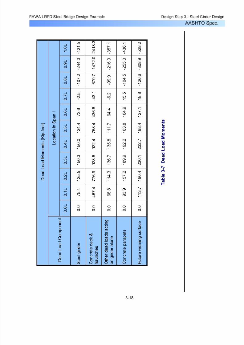
7/29/2019 LRFD steel design.pdf
http://slidepdf.com/reader/full/lrfd-steel-designpdf 129/646
1 . 0 L
- 4 2 1 . 5
- 2 4 1 8 . 3
- 3 5 7 . 1
- 4 3 6 . 1
- 5 2 8 . 2
0 . 9 L
- 2 4 4 . 0
- 1 4 7 2 . 0
- 2 1 6 . 9
- 2 5 5 . 0
- 3 0 8 . 9
0 . 8 L
- 1 0 7 . 2
- 6 7 9 . 7
- 9 9 . 9
- 1 0 4 . 5
- 1 2 6 . 6
0 . 7 L
- 2 . 5
- 4 3 . 1
- 6 . 2
1 5 . 5
1 8 . 8
0 . 6 L
7 3 . 6
4 3 6 . 6
6 4 . 4
1 0 4 . 9
1 2 7 . 1
0 . 5 L
1 2 4 . 4
7 5 8 . 4
1 1 1 . 7
1 6 3 . 8
1 9 8 . 4
0 . 4 L
1 5 0 . 0
9 2 2 . 4
1 3 5 . 8
1 9 2 . 2
2 3 2 . 7
0 . 3 L
1 5 0 . 3
9 2 8 . 6
1 3 6 . 7
1 8 9 . 9
2 3 0 . 1
0 . 2 L
1
2 5 . 5
7
7 6 . 9
1
1 4 . 3
1
5 7 . 2
1
9 0 . 4
0 . 1 L
7 5 . 4
4 6 7 . 4
6 8 . 8
9 3 . 9
1 1 3 . 7
0 . 0 L
0 . 0
0 . 0
0 . 0
0 . 0
0 . 0
T a
b l e 3 - 7
D e a d L o a d M o m e n t s
C o n c r e t e d e c k &
h a u n c h e s
O t h e r d e a d l o a d s a c t i n g
o n g i r d e r a l o
n e
C o n c r e t e p a r a p e t s
F u t u r e w e a r i n g s u r f a c e
D e a d L o a d M o m e n t s ( K i p - f e e t )
L o c a t i o n i n S p a n 1
D e a d L o a d
C o m p o n e n t
S t e e l g i r d e r
3-18

7/29/2019 LRFD steel design.pdf
http://slidepdf.com/reader/full/lrfd-steel-designpdf 130/646
1 . 0 L
- 1 6 . 8 4
- 8 5 . 1 8
- 1 2 . 6 5
- 1 6 . 3 6
- 1 9 . 8 2
0 . 9 L
- 1 2 . 7 4
- 7 2 . 5 2
- 1 0 . 7 2
- 1 3 . 8 2
- 1 6 . 7 4
0 . 8 L
- 1 0 . 0 6
- 5 9 . 5 4
- 8 . 7 8
- 1 1 . 2 7
- 1 3 . 6 5
0 . 7 L
- 7 . 3 9
- 4 6 . 5 5
- 6 . 8 5
- 8 . 7 3
- 1 0 . 5 7
0 . 6 L
- 5 . 2 9
- 3 3 . 4 0
- 4 . 9 1
- 6 . 1 8
- 7 . 4 9
0 . 5 L
- 3 . 1 8
- 2 0 . 2 4
- 2 . 9 8
- 3 . 6 3
- 4 . 4 0
0 . 4 L
- 1 . 0 8
- 7 . 0 9
- 1 . 0 4
- 1 . 0 9
- 1 . 3 2
0 . 3 L
1 . 0 2
6 . 0 6
0 . 8 9
1 . 4 6
1 . 7 7
0
. 2 L
3
. 1 2
1
9 . 2 2
2
. 8 3
4
. 0 0
4
. 8 5
0 . 1 L
5 . 2 3
3 2 . 3 7
4 . 7 6
6 . 5 5
7 . 9 3
0 . 0 L
7 . 3 3
4 5 . 5 3
6 . 7 0
9 . 1 0
1 1 . 0 2
D e a d L o a d S h e a r s ( K i p s )
L o c a t i o n i n S p
a n 1
D e a d L o a d C
o m p o n e n t
S t e e l g i r d e r
T a
b l e 3 - 8
D e a d L o a d S h e a r s
C o n c r e t e d e c k &
h a u n c h e s
O t h e r d e a d l o a d s a c t i n g
o n g i r d e r a l o n
e
C o n c r e t e p a r a
p e t s
F u t u r e w e a r i n
g s u r f a c e
3-19

7/29/2019 LRFD steel design.pdf
http://slidepdf.com/reader/full/lrfd-steel-designpdf 131/646
Design Step 3.5 - Compute Live Load Effects
LRFD Live Load
There are several differences between the live loadused in Allowable Stress Design (ASD) or LoadFactor Design (LFD) and the live load used in Loadand Resistance Factor Design (LRFD). Some of themore significant differences are:
In ASD and LFD, the basic live load designation is•HS20 or HS25. In LRFD, the basic live loaddesignation is HL-93.In ASD and LFD, the live load consists of either a•truck load or a lane load and concentrated loads.In LRFD, the load consists of a design truck or tandem, combined with a lane load.In ASD and LFD, the two concentrated loads are•combined with lane load to compute the maximumnegative live load moment. In LRFD, 90% of theeffect of two design trucks at a specified distanceis combined with 90% of the lane load to computethe maximum negative live load moment.In ASD and LFD, the term "impact" is used for the•dynamic interaction between the bridge and themoving vehicles. In LRFD, the term "dynamic load
allowance" is used instead of "impact."In ASD and LFD, impact is applied to the entire•live load. In LRFD, dynamic load allowance isapplied only to the design truck and design tandem.
For additional information about the live load used in
LRFD, refer to S3.6 and C3.6 .
The girder must also be designed to resist the live load effects. Thelive load consists of an HL-93 loading. Similar to the dead load, the
live load moments and shears for an HL-93 loading can be obtainedfrom an analysis computer program.
S3.6.1.2
Based on Table 3-3, for all limit states other than fatigue and fracture,the dynamic load allowance, IM, is as follows:
S3.6.2.1
IM 0.33=
3-20

7/29/2019 LRFD steel design.pdf
http://slidepdf.com/reader/full/lrfd-steel-designpdf 132/646
OKftL 120=
20 L≤ 240≤
OKints 8.0=
4.5 ts≤ 12.0≤
OKftS 9.75=
3.5 S≤ 16.0≤
STable
4.6.2.2.2b-1
Check the range of applicability as follows:
S4.6.2.2.1
After the longitudinal stiffness parameter is computed, STable
4.6.2.2.1-1 is used to find the letter corresponding with thesuperstructure cross section. The letter corresponding withthe superstructure cross section in this design example is "a."
If the superstructure cross section does not correspond withany of the cross sections illustrated in STable 4.6.2.2.1-1, then
the bridge should be analyzed as presented in S4.6.3.
Based on cross section "a," STables 4.6.2.2.2b-1 and
4.6.2.2.2.3a-1 are used to compute the distribution factors for moment and shear, respectively.
Table 3-9 Longitudinal Stiffness Parameter
Region A Region B Region C Weighted
(Pos. Mom.) (Intermediate) (At Pier) Average *
Length (Feet) 84 24 12
n 8 8 8
I (Inches4) 22,114.8 34,639.8 65,426.6
A (Inches2) 48.000 63.750 100.500
eg (Inches) 36.523 35.277 35.532
Kg (Inches4) 689,147 911,796 1,538,481 818,611
Longitudinal Stiffness Parameter, Kg
Kg n I A eg2⋅+( )⋅= eg
S4.6.2.2.1First, the longitudinal stiffness parameter, Kg, must be computed:
S4.6.2.2.2 The live load distribution factors for moment for an interior girder arecomputed as follows:
3-21

7/29/2019 LRFD steel design.pdf
http://slidepdf.com/reader/full/lrfd-steel-designpdf 133/646
lanesgint_shear_2 0.935=
gint_shear_2 0.2S
12+
S
35
⎛ ⎝
⎞ ⎠
2.0
−=
STable
4.6.2.2.3a-1
For two or more design lanes loaded, the distribution of live loadper lane for shear in interior beams is as follows:
lanesgint_shear_1 0.750=
gint_shear_1 0.36S
25.0+=
STable
4.6.2.2.3a-1
For one design lane loaded, the distribution of live load per lanefor shear in interior beams is as follows:
STable
4.6.2.2.3a-1
The live load distribution factors for shear for an interior girder arecomputed in a similar manner. The range of applicability is similar to that for moment.
lanesgint_moment_2 0.696=
gint_moment_2 0.075S
9.5
⎛ ⎝
⎞ ⎠
0.6S
L
⎛ ⎝
⎞ ⎠
0.2 Kg
12.0 L⋅ ts( )3⋅
⎡
⎣
⎤
⎦
0.1
+=
STable
4.6.2.2.2b-1
For two or more design lanes loaded, the distribution of liveload per lane for moment in interior beams is as follows:
lanesgint_moment_1 0.472=
gint_moment_1 0.06S
14
⎛ ⎝
⎞ ⎠
0.4S
L
⎛ ⎝
⎞ ⎠
0.3 Kg
12.0L ts( )3⋅
⎡⎢⎣
⎤⎥⎦
0.1
+=
STable
4.6.2.2.2b-1
For one design lane loaded, the distribution of live load per lanefor moment in interior beams is as follows:
OKin4
Kg 818611=10000 Kg≤ 7000000≤
OKNb 5=
Nb 4≥
3-22

7/29/2019 LRFD steel design.pdf
http://slidepdf.com/reader/full/lrfd-steel-designpdf 134/646
lanes (for strength limit state)gext_moment_1 0.892=
gext_moment_1 gext_moment_1 Multiple_presence_factor ⋅=
Multiple_presence_factor 1.20=
lanesgext_moment_1 0.744=
gext_moment_1
0.5( ) 4.25 ft⋅( )⋅ 0.5( ) 10.25 ft⋅( )⋅+9.75 ft⋅=
Figure 3-5 Lever Rule
Assumed
Hinge
0.5P 0.5P
6'-0"
2'-0"
4'-3"
3'-11 ¼"9'-9"
1'-5 ¼"
STable
4.6.2.2.2d-1
For one design lane loaded, the distribution of live load per lanefor moment in exterior beams is computed using the lever rule,as follows:
OKftde 2.50=
1.0− de≤ 5.5≤
STable
4.6.2.2.2d-1
Check the range of applicability as follows:
de 2.50ft=
The distance, de, is defined as the distance between the webcenterline of the exterior girder and the interior edge of the curb.For this design example, based on Figure 3-2:
S4.6.2.2.2 This design example is based on an interior girder. However, for illustrative purposes, the live load distribution factors for an exterior girder are computed below, as follows:
S4.6.2.2.2e,
S4.6.2.2.3c
Since this bridge has no skew, the skew correction factor doesnot need to be considered for this design example.
3-23
7/29/2019 LRFD steel design.pdf
http://slidepdf.com/reader/full/lrfd-steel-designpdf 135/646
S4.6.2.2.2d In beam-slab bridge cross-sections with diaphragms or cross-frames,the distribution factor for the exterior beam can not be taken to be lessthan that which would be obtained by assuming that the cross-section
deflects and rotates as a rigid cross-section. CEquation 4.6.2.2.2d-1 provides one approximate approach to satisfy this requirement. The
multiple presence factor provisions of S3.6.1.1.2 must be appliedwhen this equation is used.
lanesgext_shear_2 0.795=
gext_shear_2 e gint_shear_2⋅=
e 0.850=e 0.6de
10+=
STable
4.6.2.2.3b-1
For two or more design lanes loaded, the distribution of liveload per lane for shear in exterior beams is as follows:
lanes (for strength limit state)gext_shear_1 0.892=
gext_shear_1 gext_shear_1 Multiple_presence_factor ⋅=
Multiple_presence_factor 1.20=
lanesgext_shear_1 0.744=
gext_shear_10.5( ) 4.25 ft⋅( )⋅ 0.5( ) 10.25 ft⋅( )⋅+
9.75 ft⋅=
STable
4.6.2.2.3b-1
For one design lane loaded, the distribution of live load per lanefor shear in exterior beams is computed using the lever rule, asillustrated in Figure 3-5 and as follows:
STable
4.6.2.2.3b-1
The live load distribution factors for shear for an exterior girder arecomputed in a similar manner. The range of applicability is similar to that for moment.
lanesgext_moment_2 0.727=
gext_moment_2 e gint_moment_2⋅=
e 1.045=e 0.77de
9.1+=
STable
4.6.2.2.2d-1
For two or more design lanes loaded, the distribution of live loadper lane for moment in exterior beams is as follows:
3-24

7/29/2019 LRFD steel design.pdf
http://slidepdf.com/reader/full/lrfd-steel-designpdf 136/646

7/29/2019 LRFD steel design.pdf
http://slidepdf.com/reader/full/lrfd-steel-designpdf 137/646
1 . 0 L
9 8 3
- 2 4 5 0
3 5 . 8
- 1 3 1 . 4
0 . 9 L
8 6 5
- 1 5 9 3
3 3 . 0
- 1 1 8 .
5
0 . 8 L
1 0 0 6
- 1 0 9 7
3 2 . 1
- 1 0 5 . 1
0 . 7 L
1 3 1 8
- 9 6 6
3 3 . 5
- 9 1 . 1
0 . 6 L
1 6 2 8
- 9 6 6
3 7 . 1
- 7 6 . 7
0 . 5 L
1 8 5 7
- 9 6 8
4 2 . 5
- 6 2 . 2
0 . 4 L
1 9 0 8
- 9 0 5
4 9 . 6
- 4 7 . 8
0 . 3 L
1 7 6 6
- 7 7 7
6 1 . 0
- 3 6 . 4
0 . 2
L
1 4 2
2
- 5 8
3
7 6 . 6
- 2 9
. 1
0 . 1 L
8 3 6
- 3 2 4
9 3 . 7
- 2 8 . 7
0 . 0 L
0 0 1 1 0 . 5
- 3 3 . 8
T a b l e 3 - 1 0
L i v e L o a d E f f e c
t s
L i v e L o a d E f f e c t s ( f o r I n t e r i o r B e
a m s )
L o c a t i o n i n S p a n 1
M a x i m u
m
n e g a t i v e s h e a r
( k i p s )
L i v e
L o a d
E f f e c t
M a x i m u
m
p o s i t i v e
m o m e n t ( K - f t )
M a x i m u
m
n e g a t i v e
m o m e n t ( K - f t )
M a x i m u
m
p o s i t i v e
s h e a r
( k i p s )
3-26
7/29/2019 LRFD steel design.pdf
http://slidepdf.com/reader/full/lrfd-steel-designpdf 138/646
The design live load values for HL-93 loading, as presented in theprevious table, are computed based on the product of the live loadeffect per lane and live load distribution factor. These values alsoinclude the effects of dynamic load allowance. However, it isimportant to note that the dynamic load allowance is applied only tothe design truck or tandem. The dynamic load allowance is notapplied to pedestrian loads or to the design lane load.
S3.6.1,
S3.6.2,
S4.6.2.2
Design Step 3.6 - Combine Load Effects
After the load factors and load combinations have beenestablished (see Design Step 3.1), the section properties havebeen computed (see Design Step 3.3), and all of the load effectshave been computed (see Design Steps 3.4 and 3.5), the forceeffects must be combined for each of the applicable limit states.
For this design example, η equals 1.00. (For more detailedinformation about η, refer to Design Step 1.)
Based on the previous design steps, the maximum positivemoment (located at 0.4L) for the Strength I Limit State is computedas follows:
S1.3
S3.4.1
LFDC 1.25=
MDC 150.0K ft⋅ 922.4K ft⋅+ 135.8K ft⋅+192.2K ft⋅+
...=
MDC 1400.4K ft⋅=
LFDW 1.50=
MDW 232.7K ft⋅=
LFLL 1.75=
MLL 1908K ft⋅=
Mtotal LFDC MDC⋅ LFDW MDW⋅+ LFLL MLL⋅+=
Mtotal 5439 K ft⋅=
3-27

7/29/2019 LRFD steel design.pdf
http://slidepdf.com/reader/full/lrfd-steel-designpdf 139/646
f LL 1.63− ksi=f LL
MLL−12 in⋅
ft
⎛ ⎝
⎞ ⎠
⋅
Stopgdr =
Stopgdr 14010.3in3=
MLL 1908 K ft⋅=
Live load (HL-93) and dynamic load allowance:
f fws 0.82− ksi=f fws
Mfws−12 in⋅
ft
⎛ ⎝
⎞ ⎠
⋅
Stopgdr =
Stopgdr 3398.4in3
=Mfws 232.7K ft⋅=
Future wearing surface dead load (composite):
f parapet 0.68− ksi=f parapet
Mparapet−12 in⋅
ft
⎛ ⎝
⎞ ⎠
⋅
Stopgdr =
Stopgdr 3398.4in3=Mparapet 192.2K ft⋅=
Parapet dead load (composite):
f noncompDL 19.44− ksi=
f noncompDL
MnoncompDL−12 in⋅
ft
⎛ ⎝
⎞ ⎠
⋅
Stopgdr =
Stopgdr 745.9 in3⋅=
MnoncompDL 1208.2K ft⋅=
MnoncompDL 150.0K ft⋅ 922.4K ft⋅+ 135.8K ft⋅+=
Noncomposite dead load:
Similarly, the maximum stress in the top of the girder due to positivemoment (located at 0.4L) for the Strength I Limit State is computed asfollows:
3-28

7/29/2019 LRFD steel design.pdf
http://slidepdf.com/reader/full/lrfd-steel-designpdf 140/646
Multiplying the above stresses by their respective loadfactors and adding the products results in the followingcombined stress for the Strength I Limit State:
S3.4.1
f Str LFDC f noncompDL⋅( ) LFDC f parapet⋅( )+LFDW f fws⋅( ) LFLL f LL⋅( )++
...=
f Str 29.24− ksi=
Similarly, all of the combined moments, shears, and flexural stressescan be computed at the controlling locations. A summary of thosecombined load effects for an interior beam is presented in thefollowing three tables, summarizing the results obtained using theprocedures demonstrated in the above computations.
Summary of Unfactored Values:
Noncomposite DL 1208 16.95 -19.44 0.00
Parapet DL 192 1.93 -0.68 -0.05
FWS DL 233 2.34 -0.82 -0.06
LL - HL-93 1908 17.52 -1.63 -0.67
LL - Fatigue 563 5.17 -0.48 -0.20
Summary of Factored Values:
Strength I 5439 57.77 -29.24 -1.33
Service II 4114 44.00 -23.06 -0.99
Fatigue 422 3.87 -0.36 -0.15
Combined Effects at Location of Maximum Positive Moment
LoadingMoment
(K-ft)
f botgdr
ksi
f topgdr
ksi
f topslab
(ksi)
f topslab
ksi
Limit State
Moment
(K-ft)
f botgdr
(ksi)
f topgdr
(ksi)
Table 3-11 Combined Effects at Location of
Maximum Positive Moment
As shown in the above table, the Strength I Limit State elastic stressin the bottom of the girder exceeds the girder yield stress.
However, for this design example, this value is not used because of the local yielding that occurs at this section.
3-29
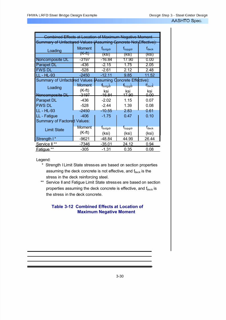
7/29/2019 LRFD steel design.pdf
http://slidepdf.com/reader/full/lrfd-steel-designpdf 141/646
Noncomposite DL -3197 -16.84 17.90 0.00
Parapet DL -436 -2.15 1.75 2.05
FWS DL -528 -2.61 2.12 2.48
LL - HL-93 -2450 -12.11 9.85 11.52
Noncomposite DL -3197 -16.84 17.90 0.00
Parapet DL -436 -2.02 1.15 0.07
FWS DL -528 -2.44 1.39 0.08
LL - HL-93 -2450 -10.55 2.83 0.61LL - Fatigue -406 -1.75 0.47 0.10
Strength I * -9621 -48.84 44.99 26.44
Service II ** -7346 -35.01 24.12 0.94
Fatigue ** -305 -1.31 0.35 0.08
Legend:
* Strength I Limit State stresses are based on section properties
assuming the deck concrete is not effective, and f deck is the
stress in the deck reinforcing steel.
** Service II and Fatigue Limit State stresses are based on section
properties assuming the deck concrete is effective, and f deck is
the stress in the deck concrete.
Summary of Unfactored Values (Assuming Concrete Effective):
LoadingMoment
(K-ft)
f botgdr
ksi
f topgdr
ksi
f deck
ksi
Summary of Factored Values:
Moment
(K-ft)
f botgdr
(ksi)
f topgdr
(ksi)
f deck
(ksi)Limit State
Combined Effects at Location of Maximum Negative Moment
LoadingMoment
(K-ft)
f botgdr
(ksi)
f topgdr
(ksi)
f deck
(ksi)
Summary of Unfactored Values (Assuming Concrete Not Effective):
Table 3-12 Combined Effects at Location of
Maximum Negative Moment
3-30
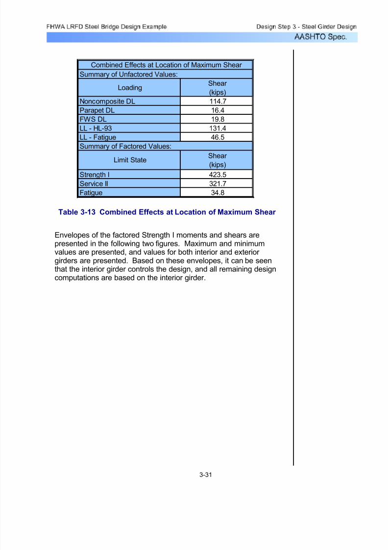
7/29/2019 LRFD steel design.pdf
http://slidepdf.com/reader/full/lrfd-steel-designpdf 142/646
Summary of Unfactored Values:
Noncomposite DL 114.7
Parapet DL 16.4
FWS DL 19.8
LL - HL-93 131.4
LL - Fatigue 46.5
Summary of Factored Values:
Strength I 423.5
Service II 321.7
Fatigue 34.8
Combined Effects at Location of Maximum Shear
Loading
Limit State
Shear
(kips)
Shear
(kips)
Table 3-13 Combined Effects at Location of Maximum Shear
Envelopes of the factored Strength I moments and shears arepresented in the following two figures. Maximum and minimumvalues are presented, and values for both interior and exterior girders are presented. Based on these envelopes, it can be seenthat the interior girder controls the design, and all remaining designcomputations are based on the interior girder.
3-31

7/29/2019 LRFD steel design.pdf
http://slidepdf.com/reader/full/lrfd-steel-designpdf 143/646
F i g u r e 3 - 6
E n v e l o
p e o f S t r e n g t h I M o m e n t s
3-32
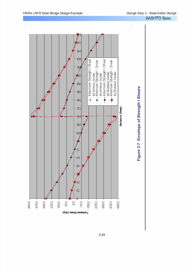
7/29/2019 LRFD steel design.pdf
http://slidepdf.com/reader/full/lrfd-steel-designpdf 144/646
F i g u r e 3 - 7
E n v e l o p e o f S t r e n g t h I S h
e a r s
3-33
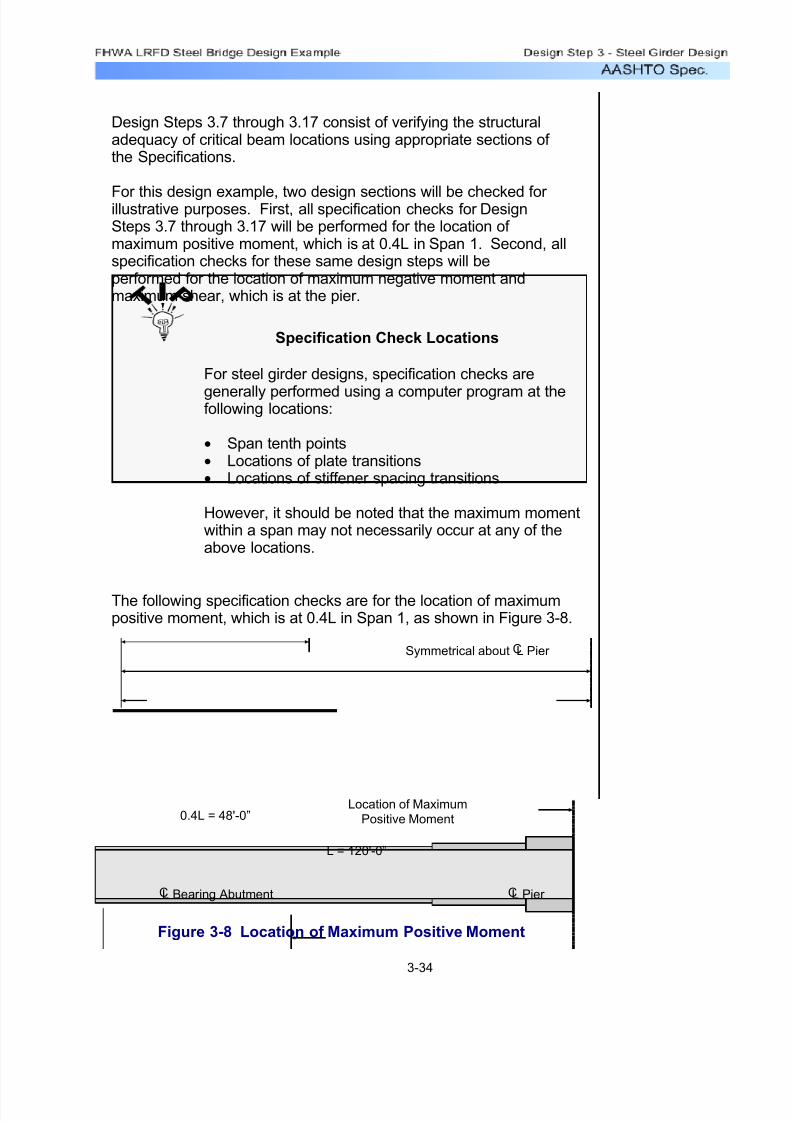
7/29/2019 LRFD steel design.pdf
http://slidepdf.com/reader/full/lrfd-steel-designpdf 145/646
Design Steps 3.7 through 3.17 consist of verifying the structuraladequacy of critical beam locations using appropriate sections of the Specifications.
For this design example, two design sections will be checked for illustrative purposes. First, all specification checks for DesignSteps 3.7 through 3.17 will be performed for the location of maximum positive moment, which is at 0.4L in Span 1. Second, allspecification checks for these same design steps will beperformed for the location of maximum negative moment andmaximum shear, which is at the pier.
Specification Check Locations
For steel girder designs, specification checks are
generally performed using a computer program at thefollowing locations:
Span tenth points•Locations of plate transitions•Locations of stiffener spacing transitions•
However, it should be noted that the maximum momentwithin a span may not necessarily occur at any of theabove locations.
The following specification checks are for the location of maximumpositive moment, which is at 0.4L in Span 1, as shown in Figure 3-8.
0.4L = 48'-0”
L = 120'-0”
L Bearing Abutment L Pier
Location of Maximum
Positive Moment
CC
Symmetrical about L Pier C
Figure 3-8 Location of Maximum Positive Moment
3-34

7/29/2019 LRFD steel design.pdf
http://slidepdf.com/reader/full/lrfd-steel-designpdf 146/646
(see Figure 3-4)tbotfl 0.875in=
(see Figure 3-4)Dweb 54in=
(see Figure 3-4)ttopfl 0.625in=
(see Table 3-11)f topgdr 29.24− ksi⋅=
(see Table 3-11and explanation
below table)
f botgdr 57.77 ksi⋅=
S6.10.3.1.4aFor the Strength I limit state at 0.4L in Span 1 (the location of maximum positive moment):
2 Dc⋅
tw6.77
E
f c⋅≤ 200≤
S6.10.2.2 The second section proportion check relates to the webslenderness. For a section without longitudinal stiffeners, the webmust be proportioned such that:
OKIyc
Iy0.416=
Iy 343.6in4
=
Iy0.625 in⋅ 14 in⋅( )
3⋅12
54 in⋅ 12
in⋅⎛ ⎝
⎞ ⎠
3⋅
12+
0.875 in⋅ 14 in⋅( )3⋅
12+=
Iyc 142.9in4=Iyc
0.625 in⋅ 14 in⋅( )3⋅
12=
0.1Iyc
Iy≤ 0.9≤
S6.10.2.1
S6.10.2 Several checks are required to ensure that the proportions of thetrial girder section are within specified limits.
The first section proportion check relates to the general proportionsof the section. The flexural components must be proportioned suchthat:
Design Step 3.7 - Check Section Proportion Limits - Positive
Moment Region
3-35
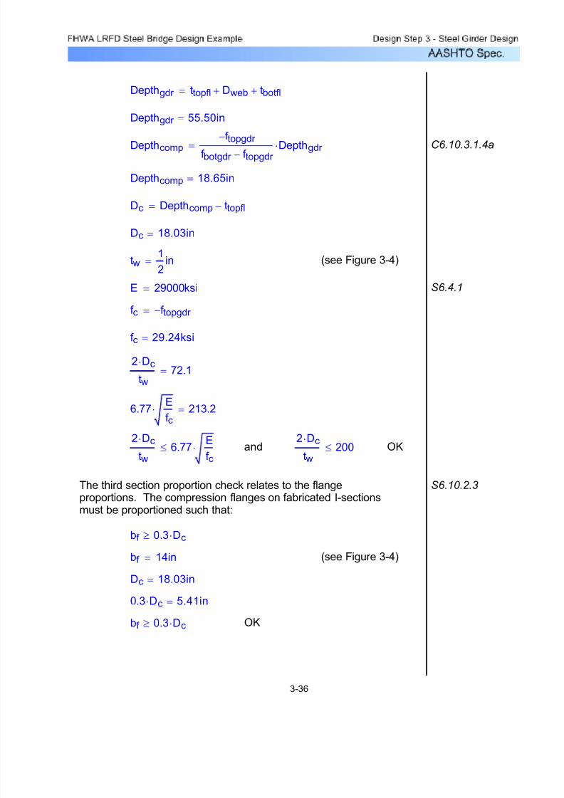
7/29/2019 LRFD steel design.pdf
http://slidepdf.com/reader/full/lrfd-steel-designpdf 147/646
OKbf 0.3 Dc⋅≥
0.3 Dc⋅ 5.41in=
Dc 18.03in=(see Figure 3-4)bf 14in=
bf 0.3 Dc⋅≥
S6.10.2.3The third section proportion check relates to the flangeproportions. The compression flanges on fabricated I-sectionsmust be proportioned such that:
OK2 Dc⋅
tw200≤and
2 Dc⋅
tw6.77
E
f c⋅≤
6.77E
f c
⋅ 213.2=
2 Dc⋅
tw72.1=
f c 29.24ksi=
f c f topgdr −=
S6.4.1E 29000ksi=
(see Figure 3-4)tw1
2in=
Dc 18.03in=
Dc Depthcomp ttopfl−=
Depthcomp 18.65in=
C6.10.3.1.4aDepthcomp f topgdr −f botgdr f topgdr −
Depthgdr ⋅=
Depthgdr 55.50in=
Depthgdr ttopfl Dweb+ tbotfl+=
3-36
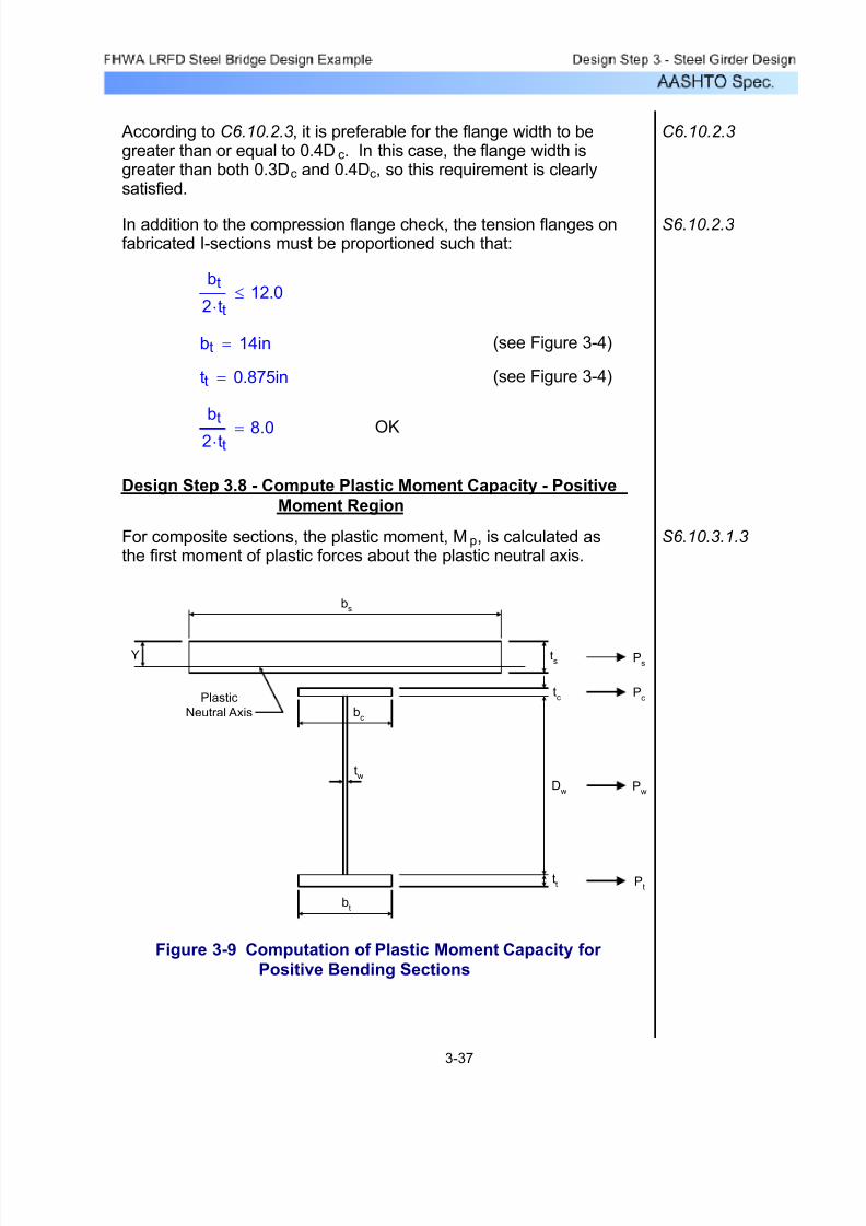
7/29/2019 LRFD steel design.pdf
http://slidepdf.com/reader/full/lrfd-steel-designpdf 148/646
Figure 3-9 Computation of Plastic Moment Capacity for
Positive Bending Sections
bs
ts
tc
bc
tw
bt
Dw
tt
Y
Plastic
Neutral Axis
Ps
Pc
Pw
Pt
S6.10.3.1.3For composite sections, the plastic moment, Mp, is calculated asthe first moment of plastic forces about the plastic neutral axis.
Design Step 3.8 - Compute Plastic Moment Capacity - Positive
Moment Region
OK
bt
2 tt⋅ 8.0=
(see Figure 3-4)tt 0.875in=
(see Figure 3-4)bt 14in=
bt
2 tt⋅12.0≤
S6.10.2.3In addition to the compression flange check, the tension flanges onfabricated I-sections must be proportioned such that:
C6.10.2.3 According to C6.10.2.3, it is preferable for the flange width to begreater than or equal to 0.4Dc. In this case, the flange width isgreater than both 0.3Dc and 0.4Dc, so this requirement is clearlysatisfied.
3-37

7/29/2019 LRFD steel design.pdf
http://slidepdf.com/reader/full/lrfd-steel-designpdf 149/646
bs 103in= ts 8.0in=
Ps 0.85 f'c⋅ bs⋅ ts⋅= Ps 2802K=
The forces in the longitudinal reinforcement may beconservatively neglected.
C6.10.3.1.3
Check the location of the plastic neutral axis, as follows: SAppendix A6.1
Pt Pw+ 1963K= Pc Ps+ 3239K=
Pt Pw+ Pc+ 2400K= Ps 2802K=
Therefore, the plastic neutral axis is located within the slab.
Y ts( )Pc Pw+ Pt+
Ps
⎛
⎝
⎞
⎠⋅= STable A6.1-1
Y 6.85 in=
Check that the position of the plastic neutral axis, as computedabove, results in an equilibrium condition in which there is no net
axial force.
Compression 0.85 f'c⋅ bs⋅ Y⋅=
Compression 2400K=
Tension Pt Pw+ Pc+=
Tension 2400K= OK
For the tension flange: SAppendix A6.1
Fyt 50ksi= bt 14in= tt 0.875in=
Pt Fyt bt⋅ tt⋅= Pt 613K=
For the web:
Fyw 50.0ksi= Dw 54in= tw 0.50in=
Pw Fyw Dw⋅ tw⋅= Pw 1350K=
For the compression flange:
Fyc 50ksi= bc 14in= tc 0.625in=
Pc Fyc bc⋅ tc⋅= Pc 438K=
For the slab:
f'c 4.0ksi=
3-38

7/29/2019 LRFD steel design.pdf
http://slidepdf.com/reader/full/lrfd-steel-designpdf 150/646
CFigure
6.10.4-1
S6.10.4.1.2 Therefore the web is deemed compact. Since this is a composite
section in positive flexure, the flexural resistance is computed asdefined by the composite compact-section positive flexural
resistance provisions of S6.10.4.2.2 .
For composite sections in positive flexure in their final condition, theprovisions of S6.10.4.1.3, S6.10.4.1.4, S6.10.4.1.6a, S6.10.4.1.7 ,
and S6.10.4.1.9 are considered to be automatically satisfied.
The section is therefore considered to be compact.
Dcp 0in=
Since the plastic neutral axis is located within the slab,
2 Dcp⋅
tw3.76
E
Fyc⋅≤
S6.10.4.1.2
S6.10.4.1.1
The next step in the design process is to determine if the section iscompact or noncompact. This, in turn, will determine which formulaeshould be used to compute the flexural capacity of the girder.
Where the specified minimum yield strength does not exceed 70.0ksi, and the girder has a constant depth, and the girder does not
have longitudinal stiffeners or holes in the tension flange, then thefirst step is to check the compact-section web slendernessprovisions, as follows:
Design Step 3.9 - Determine if Section is Compact or
Noncompact - Positive Moment Region
Mp 7419 K ft⋅=
MpY
2Ps⋅
2 ts⋅Pc dc⋅ Pw dw⋅+ Pt dt⋅+( )+=
dt 59.08in=dttt
2Dw+ 3.5in+ ts+ Y−=
dw 31.65in=dwDw
23.5in+ ts+ Y−=
dc 4.33in=dc
tc−
2 3.5in+ ts+ Y−=
STable A6.1-1The plastic moment, Mp, is computed as follows, where d is thedistance from an element force (or element neutral axis) to theplastic neutral axis:
3-39

7/29/2019 LRFD steel design.pdf
http://slidepdf.com/reader/full/lrfd-steel-designpdf 151/646
SST 1306.8 in3⋅=
SLT 1192.7 in3
⋅=
SNC 855.5 in3
⋅=
For the bottom flange:
MD2 590K ft⋅=
MD2 1.25 192⋅ K ft⋅( ) 1.50 233⋅ K ft⋅( )+=
MD1 1510K ft⋅=
MD1 1.25 1208⋅ K ft⋅( )=
Fy 50ksi=
My MD1 MD2+ M AD+= M AD
FyMD1
SNC
MD2
SLT+
M AD
SST+=
SST
SAppendix A6.2 The yield moment, My, is computed as follows:
Rh 1.0=
S6.10.4.3.1 All design sections of this girder are homogenous. That is, thesame structural steel is used for the top flange, the web, and thebottom flange. Therefore, the hybrid factor, Rh, is as follows:
Mn 1.3 Rh⋅ My⋅= My
S6.10.4.2.2a
SFigure
C6.10.4-1
Since the section was determined to be compact, and since it is acomposite section in the positive moment region, the flexural
resistance is computed in accordance with the provisions of S6.10.4.2.2 .
This is neither a simple span nor a continuous span with compactsections in the negative flexural region over the interior supports.(This will be proven in the negative flexure region computations of this design example.) Therefore, the nominal flexural resistance isdetermined using the following equation, based on the approximatemethod:
Design Step 3.10 - Design for Flexure - Strength Limit State -
Positive Moment Region
3-40
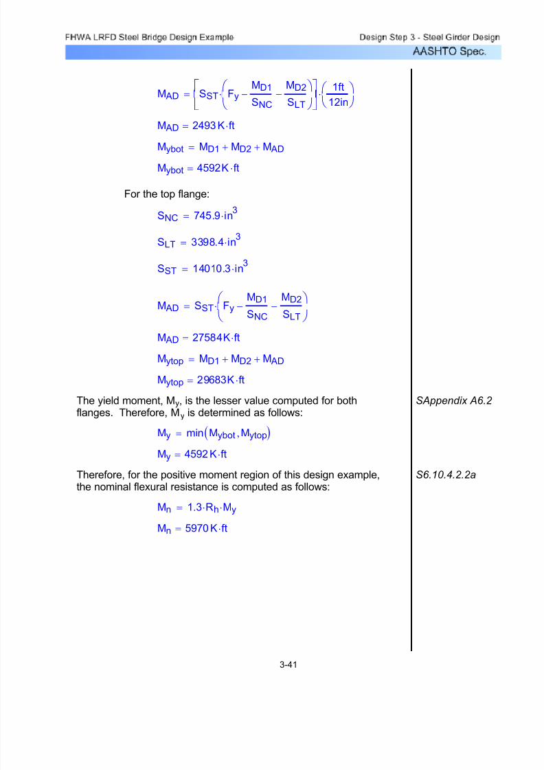
7/29/2019 LRFD steel design.pdf
http://slidepdf.com/reader/full/lrfd-steel-designpdf 152/646

7/29/2019 LRFD steel design.pdf
http://slidepdf.com/reader/full/lrfd-steel-designpdf 153/646
D' Dp≤ 5 D'⋅≤ S6.10.4.2.2a
Mn5 Mp⋅ 0.85 My⋅−
4
0.85 My⋅ Mp−
4
Dp
D'
⎛
⎝
⎞
⎠⋅+=
Mn 7326 K ft⋅=
Therefore, use Mn 5970 K⋅ ft⋅=
The ductility requirement in S6.10.4.2.2b is checked as follows: S6.10.4.2.2b
Dp
D'1.1=
Dp
D'5≤ OK
The factored flexural resistance, Mr , is computed as follows: S6.10.4
φf 1.00= S6.5.4.2
Mr φf Mn⋅=
Mr 5970 K ft⋅=
In addition, the nominal flexural resistance can not be taken to begreater than the applicable value of Mn computed from either
SEquation 6.10.4.2.2a-1 or 6.10.4.2.2a-2 .
S6.10.4.2.2a
Dp Y= Dp 6.85in=
S6.10.4.2.2bD' β
d ts+ th+( )7.5
⋅=th
β 0.7= for Fy = 50 ksi
d Depthgdr = d 55.50 in=
ts 8.0in=
th 3.5 in⋅ 0.625 in⋅−= th 2.875in=
D' βd ts+ th+( )
7.5⋅=
D' 6.19in=
5 D'⋅ 30.97in=
Therefore
3-42
7/29/2019 LRFD steel design.pdf
http://slidepdf.com/reader/full/lrfd-steel-designpdf 154/646
Available Plate Thicknesses
Based on the above computations, the flexuralresistance is approximately 10% greater than thefactored design moment, yielding a slightlyconservative design. This degree of conservatism can
generally be adjusted by changing the platedimensions as needed.
However, for this design example, the web dimensionsand the flange width were set based on the girder design requirements at the pier. In addition, the flangethicknesses could not be reduced any further due tolimitations in plate thicknesses or because such areduction would result in a specification check failure.
Available plate thicknesses can be obtained from steel
fabricators. As a rule of thumb, the following platethicknesses are generally available from steelfabricators:
3/16" to 3/4" - increments of 1/16"3/4" to 1 1/2" - increments of 1/8"1 1/2" to 4" - increments of 1/4"
OKMr 5970 K ft⋅=
Σηi γ i⋅ Mi⋅ 5439 K⋅ ft⋅=Σηi γ i⋅ Mi⋅ 5439 K⋅ ft⋅=Therefore
Σγi Mi⋅ 5439K ft⋅=Σγi Mi⋅ 5439K ft⋅=
As computed in Design Step 3.6,
η i 1.00=
For this design example,
Σηi γ i⋅ Mi⋅ Mr ≤
or in this case:
Σηi γ i⋅ Qi⋅ Rr ≤
S1.3.2.1The positive flexural resistance at this design section is checkedas follows:
3-43

7/29/2019 LRFD steel design.pdf
http://slidepdf.com/reader/full/lrfd-steel-designpdf 155/646
Design Step 3.11 - Design for Shear - Positive Moment Region
Shear must be checked at each section of the girder. However,shear is minimal at the location of maximum positive moment, and
it is maximum at the pier.
Therefore, for this design example, the required shear designcomputations will be presented later for the girder design sectionat the pier.
S6.10.7
It should be noted that in end panels, the shear is limited to either the shear yield or shear buckling in order to provide an anchor for the tension field in adjacent interior panels. Tension field is notallowed in end panels. The design procedure for shear in the end
panel is presented in S6.10.7.3.3c .
S6.10.7.3.3c
Design Step 3.12 - Design Transverse Intermediate Stiffeners -
Positive Moment Region
The girder in this design example has transverse intermediatestiffeners. Transverse intermediate stiffeners are used to increasethe shear resistance of the girder.
As stated above, shear is minimal at the location of maximumpositive moment but is maximum at the pier. Therefore, therequired design computations for transverse intermediate stiffeners
will be presented later for the girder design section at the pier.
S6.10.8.1
Design Step 3.14 - Design for Flexure - Fatigue and Fracture
Limit State - Positive Moment Region
Load-induced fatigue must be considered in a plate girder design.Fatigue considerations for plate girders may include:
1. Welds connecting the shear studs to the girder.2. Welds connecting the flanges and the web.3. Welds connecting the transverse intermediate stiffeners to the
girder.
The specific fatigue considerations depend on the uniquecharacteristics of the girder design. Specific fatigue details and
detail categories are explained and illustrated in STable
6.6.1.2.3-1 and in SFigure 6.6.1.2.3-1.
S6.6.1
STable
6.6.1.2.3-1
SFigure
6.6.1.2.3-1
3-44

7/29/2019 LRFD steel design.pdf
http://slidepdf.com/reader/full/lrfd-steel-designpdf 156/646
For this design example, fatigue will be checked for thefillet-welded connection of the transverse intermediate stiffeners tothe girder. This detail corresponds to Illustrative Example 6 in
SFigure 6.6.1.2.3-1, and it is classified as Detail Category C' in
STable 6.6.1.2.3-1.
For this design example, the fillet-welded connection of thetransverse intermediate stiffeners will be checked at the location of maximum positive moment. The fatigue detail is located at theinner fiber of the tension flange, where the transverse intermediatestiffener is welded to the flange. However, for simplicity, thecomputations will conservatively compute the fatigue stress at theouter fiber of the tension flange.
The fatigue detail being investigated in this design example is
illustrated in the following figure:
Transverse
IntermediateStiffener (Typ.) Fillet Weld (Typ.)
Figure 3-10 Load-Induced Fatigue Detail
The nominal fatigue resistance is computed as follows: S6.6.1.2.5
∆F( )n
A
N
⎛ ⎝
⎞ ⎠
1
31
2∆F( )
TH≥=
TH
for which:
STable
6.6.1.2.5-1 A 44.0 10
8⋅ ksi( )3=
N 365( ) 75( )⋅ n⋅ ADTT( )SL⋅= SLS6.6.1.2.5
n 1.0= STable
6.6.1.2.5-2
ADTTSL 3000=
3-45

7/29/2019 LRFD steel design.pdf
http://slidepdf.com/reader/full/lrfd-steel-designpdf 157/646
S6.10.6 In addition to the above fatigue detail check, fatigue requirementsfor webs must also be checked. These calculations will be
presented later for the girder design section at the pier.
OKf botgdr ∆Fn≤
f botgdr 3.87 ksi⋅=
The factored fatigue stress in the outer fiber of the tension flange atthe location of maximum positive moment was previouslycomputed in Table 3-11, as follows:
Fatigue Resistance
CTable 6.6.1.2.5-1 can be used to eliminate the needfor some of the above fatigue resistancecomputations. The above computations are presentedsimply for illustrative purposes.
∆Fn 6.00ksi=
S6.6.1.2.5 ∆Fn max
A
N
⎛
⎝
⎞
⎠
1
31
2 ∆FTH⋅,
⎡
⎣
⎤
⎦=
1
2∆FTH⋅ 6.00ksi=
A
N
⎛ ⎝
⎞ ⎠
1
3
3.77ksi=
∆FTH
12.0 ksi⋅= STable
6.6.1.2.5-3
N 82125000=
N 365( ) 75( )⋅ n⋅ ADTTSL⋅=
3-46
7/29/2019 LRFD steel design.pdf
http://slidepdf.com/reader/full/lrfd-steel-designpdf 158/646
S2.5.2.6.2 This maximum live load deflection is computed based on thefollowing:
1. All design lanes are loaded.2. All supporting components are assumed to deflect equally.3. For composite design, the design cross section includes the
entire width of the roadway.4. The number and position of loaded lanes is selected to provide
the worst effect.5. The live load portion of Service I Limit State is used.6. Dynamic load allowance is included.
7. The live load is taken from S3.6.1.3.2 .
∆max 1.43 in⋅=
S2.5.2.6.2 In addition to the check for service limit state control of permanentdeflection, the girder can also be checked for live load deflection.
Although this check is optional for a concrete deck on steelgirders, it is included in this design example.
Using an analysis computer program, the maximum live loaddeflection is computed to be the following:
OK0.95 Fyf ⋅ 47.50ksi=
Fyf 50.0ksi=
f topgdr 23.06− ksi⋅=f botgdr 44.00 ksi⋅=
The factored Service II flexural stress was previously computed inTable 3-11 as follows:
S6.10.5.2 f f 0.95Fyf ≤
S6.10.5 The girder must be checked for service limit state control of permanent deflection. This check is intended to prevent
objectionable permanent deflections due to expected severe trafficloadings that would impair rideability. Service II Limit State is usedfor this check.
The flange stresses for both steel flanges of composite sectionsmust satisfy the following requirement:
Design Step 3.15 - Design for Flexure - Service Limit State -
Positive Moment Region
3-47
7/29/2019 LRFD steel design.pdf
http://slidepdf.com/reader/full/lrfd-steel-designpdf 159/646
S6.10.4.1.9Lb Lp≤ 1.76 r t⋅E
Fyc⋅=Lb Lp≤ 1.76 r t⋅
E
Fyc⋅=
Therefore, the investigation proceeds with the noncompact sectioncompression-flange bracing provisions of S6.10.4.1.9.
bf
2 tf ⋅11.2=
(see Figure 3-4)tf 0.625in=
(see Figure 3-4)bf 14in=
bf
2 tf ⋅12.0≤
S6.10.4.1.4
S6.10.3.2 The girder must also be checked for flexure during construction.The girder has already been checked in its final condition when itbehaves as a composite section. The constructibility must also be
checked for the girder prior to the hardening of the concrete deckwhen the girder behaves as a noncomposite section.
As previously stated, a deck pouring sequence will not beconsidered in this design example. However, it is generallyimportant to consider the effects of the deck pouring sequence inan actual design because it will often control the design of the topflange in the positive moment regions of composite girders.
The investigation of the constructibility of the girder begins with thethe noncompact section compression-flange slenderness check, asfollows:
Design Step 3.16 - Design for Flexure - Constructibility Check -
Positive Moment Region
OK∆allowable 1.80in=
∆allowable
Span
800
⎛
⎝
⎞
⎠
12in
ft
⎛
⎝
⎞
⎠⋅=
Span 120 ft⋅=
S2.5.2.6.2 In the absence of other criteria, the deflection limit is as follows:
3-48

7/29/2019 LRFD steel design.pdf
http://slidepdf.com/reader/full/lrfd-steel-designpdf 160/646
Therefore, the investigation proceeds with the noncompositesection lateral torsional buckling provisions of S6.10.4.2.6 .
Lb 20.0ft=
Lp 11.46ft=Lp 1.76 r t⋅E
Fyc⋅=
Fyc 50ksi=E 29000ksi=
r t 3.24in=r tIt
At=
At 13.6in2= At tc bc⋅( )
Dc
3tw⋅
⎛ ⎝
⎞ ⎠
+=
It 143.0in4=It
tc bc3⋅
12
Dc
3tw
3⋅
12+=
tc 0.625in=bc 14.0in=
Dc
39.67in=D
c29.02in=
Dc Depthcomp ttopfl−=
Depthcomp 29.65in=
(see Figure 3-4 and Table 3-4)
Depthcomp 55.50 in⋅ 25.852 in⋅−=
For the noncomposite loads during construction:
The term, r t, is defined as the radius of gyration of a notionalsection comprised of the compression flange of the steel sectionplus one-third of the depth of the web in compression taken aboutthe vertical axis.
3-49
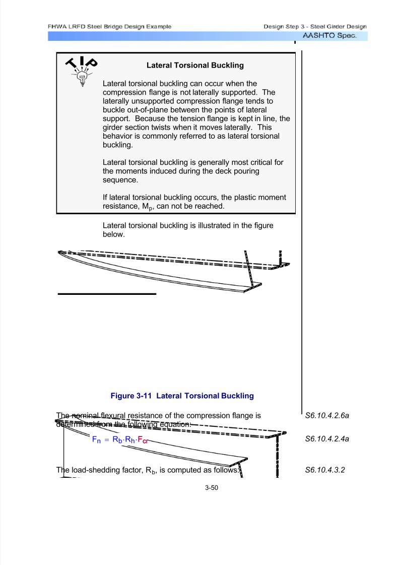
7/29/2019 LRFD steel design.pdf
http://slidepdf.com/reader/full/lrfd-steel-designpdf 161/646
Lateral Torsional Buckling
Lateral torsional buckling can occur when thecompression flange is not laterally supported. The
laterally unsupported compression flange tends tobuckle out-of-plane between the points of lateralsupport. Because the tension flange is kept in line, thegirder section twists when it moves laterally. Thisbehavior is commonly referred to as lateral torsionalbuckling.
Lateral torsional buckling is generally most critical for the moments induced during the deck pouringsequence.
If lateral torsional buckling occurs, the plastic momentresistance, Mp, can not be reached.
Lateral torsional buckling is illustrated in the figurebelow.
Figure 3-11 Lateral Torsional Buckling
The nominal flexural resistance of the compression flange isdetermined from the following equation:
S6.10.4.2.6a
Fn Rb Rh⋅ Fcr ⋅= Fcr S6.10.4.2.4a
The load-shedding factor, Rb, is computed as follows: S6.10.4.3.2
3-50
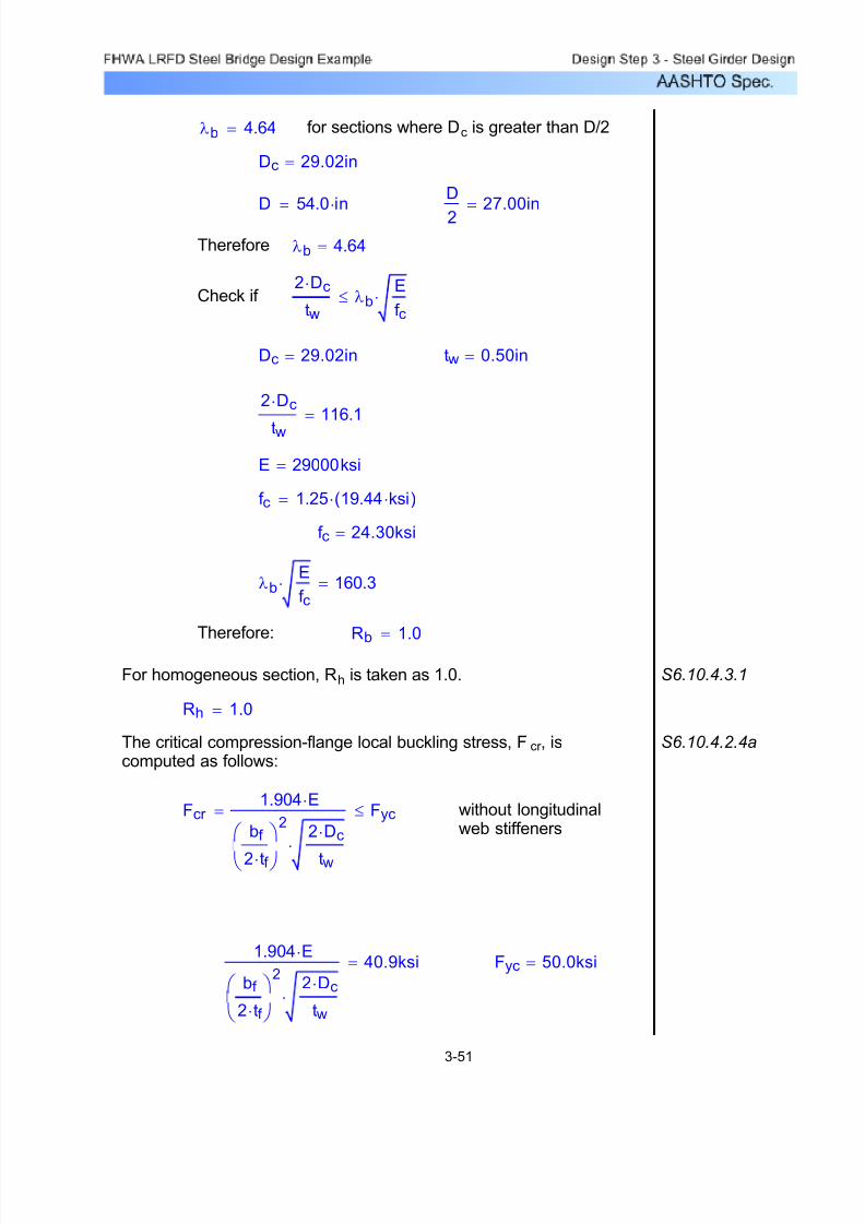
7/29/2019 LRFD steel design.pdf
http://slidepdf.com/reader/full/lrfd-steel-designpdf 162/646
Fyc 50.0ksi=1.904 E⋅
bf
2 tf ⋅
⎛
⎝
⎞
⎠
22 Dc⋅
tw⋅
40.9ksi=
without longitudinalweb stiffeners
Fcr 1.904 E⋅
bf
2 tf ⋅
⎛
⎝
⎞
⎠
22 Dc⋅
tw⋅
Fyc≤=
S6.10.4.2.4aThe critical compression-flange local buckling stress, Fcr , iscomputed as follows:
Rh 1.0=
S6.10.4.3.1For homogeneous section, Rh is taken as 1.0.
Rb
1.0=Therefore:
λbE
f c⋅ 160.3=
f c 24.30ksi=
f c 1.25 19.44 ksi⋅( )⋅=
E 29000ksi=
2 Dc⋅
tw116.1=
tw 0.50in=Dc 29.02in=
2 Dc⋅
twλb
E
f c⋅≤Check if
λb 4.64=Therefore
D
227.00in=D 54.0 in⋅=
Dc 29.02in=
for sections where Dc is greater than D/2λb 4.64=
3-51

7/29/2019 LRFD steel design.pdf
http://slidepdf.com/reader/full/lrfd-steel-designpdf 163/646
Lr 29.06ft=Lr 4.44Iyc d⋅
Sxc
E
Fyc⋅⋅=
Fyc 50.0ksi=
E 29000.0ksi=
(see Table 3-4)Sxc 745.9in3=
d 55.50 in=
Iyc 142.9in4=
Lb Lr ≤ 4.44Iyc d⋅
Sxc
E
Fyc⋅⋅=Lb Lr ≤ 4.44
Iyc d⋅
Sxc
E
Fyc⋅⋅=Check if
λbE
Fyc⋅ 111.7=
Fyc 50.0ksi=E 29000ksi=λb 4.64=
2 Dc⋅
tw116.1=
tw 0.5in=Dc 29.02in=
2 Dc⋅
twλb
E
Fyc⋅≤Check if
S6.10.4.2.6aIn addition, the nominal flexural resistance of the compressionflange should not exceed the nominal flexural resistance basedupon lateral-torsional buckling determined as follows:
Fn 40.9ksi=
Fn Rb Rh⋅ Fcr ⋅=
S6.10.4.2.4aTherefore the nominal flexural resistance of the compression flangeis determined from the following equation:
Fcr 40.9ksi=Fcr min1.904 E⋅
bf
2 tf
⋅
⎛
⎝
⎞
⎠
22 Dc⋅
tw
⋅
Fyc,⎡
⎢
⎣
⎤
⎥
⎦
=
3-52

7/29/2019 LRFD steel design.pdf
http://slidepdf.com/reader/full/lrfd-steel-designpdf 164/646
Rb Rh⋅ My⋅ 3108K ft⋅=
Cb Rb⋅ Rh⋅ My⋅ 1 0.5Lb Lp−
Lr Lp−
⎛
⎝
⎞
⎠⋅−
⎡
⎣
⎤
⎦⋅ 3258K ft⋅=
Lr 29.06ft=Lb 20.0ft=
Lp 14.28ft=Lp 1.76 r t⋅ EFyc
⋅=
Fyc 50ksi=E 29000ksi=
r t 4.04in=r tIt
At=
At 8.8in2= At tc bc⋅=
S6.10.4.2.6aIt 142.9in4
=Ittc bc
3⋅
12
=
S6.10.3.3.1
Lb 20.0ft=
Therefore:
Mn Cb Rb⋅ Rh⋅ My⋅ 1 0.5L
bL
p−
Lr Lp−⎛ ⎝ ⎞ ⎠−⎡⎣ ⎤⎦⋅ Rb Rh⋅ My⋅≤= Cb S6.10.4.2.6a
The moment gradient correction factor, Cb, is computed as follows: S6.10.4.2.5a
Cb 1.75 1.05Pl
Ph
⎛
⎝
⎞
⎠⋅− 0.3
Pl
Ph
⎛
⎝
⎞
⎠
2
⋅+ Kb≤= Kb
Use:Pl
Ph0.5=
Pl
Ph0.5= (based on analysis)
1.75 1.05 0.5( )⋅− 0.3 0.5( )2
⋅+ 1.30=
Kb 1.75=
Therefore Cb 1.30=
My 50 ksi⋅( ) 745.98⋅ in3⋅= My 3108K ft⋅=
3-53
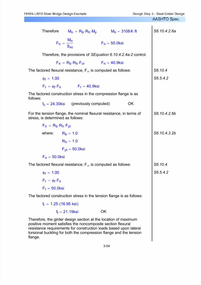
7/29/2019 LRFD steel design.pdf
http://slidepdf.com/reader/full/lrfd-steel-designpdf 165/646
For the tension flange, the nominal flexural resistance, in terms of stress, is determined as follows:
S6.10.4.2.6b
Fn Rb Rh⋅ Fyt⋅=
where: Rb 1.0= S6.10.4.3.2b
Rh 1.0=
Fyt 50.0ksi=Fn 50.0ksi=
The factored flexural resistance, Fr , is computed as follows: S6.10.4
φf 1.00= S6.5.4.2
Fr φf Fn⋅=
Fr 50.0ksi=
The factored construction stress in the tension flange is as follows:
f t 1.25 16.95 ksi⋅( )⋅=
f t 21.19ksi= OK
Therefore, the girder design section at the location of maximumpositive moment satisfies the noncomposite section flexuralresistance requirements for construction loads based upon lateraltorsional buckling for both the compression flange and the tensionflange.
Therefore Mn Rb Rh⋅ My⋅= Mn 3108 K ft⋅= S6.10.4.2.6a
FnMn
Sxc= Fn 50.0ksi=
Therefore, the provisions of SEquation 6.10.4.2.4a-2 control.
Fn Rb Rh⋅ Fcr ⋅= Fn 40.9ksi=
The factored flexural resistance, Fr , is computed as follows: S6.10.4
φf 1.00= S6.5.4.2
Fr φf Fn⋅= Fr 40.9ksi=
The factored construction stress in the compression flange is as
follows:f c 24.30ksi= (previously computed) OK
3-54
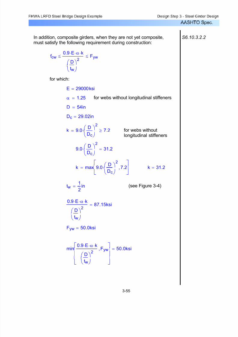
7/29/2019 LRFD steel design.pdf
http://slidepdf.com/reader/full/lrfd-steel-designpdf 166/646
min0.9 E⋅ α⋅ k⋅
D
tw
⎛ ⎝
⎞ ⎠
2Fyw,
⎡
⎢
⎣
⎤
⎥
⎦
50.0ksi=
Fyw 50.0ksi=
0.9 E⋅ α⋅ k⋅
D
tw
⎛ ⎝
⎞ ⎠
287.15ksi=
(see Figure 3-4)tw1
2in=
k 31.2=k max 9.0D
Dc
⎛ ⎝
⎞ ⎠
2
⋅ 7.2,⎡
⎣
⎤
⎦=
9.0D
Dc
⎛ ⎝
⎞ ⎠
2
⋅ 31.2=
for webs withoutlongitudinal stiffeners
k 9.0D
Dc
⎛ ⎝
⎞ ⎠
2
⋅ 7.2≥=
Dc 29.02in=
D 54in=
for webs without longitudinal stiffenersα 1.25=
E 29000ksi=
for which:
f cw
0.9 E⋅ α⋅ k⋅
D
tw
⎛ ⎝
⎞ ⎠
2≤ F
yw≤
S6.10.3.2.2 In addition, composite girders, when they are not yet composite,must satisfy the following requirement during construction:
3-55

7/29/2019 LRFD steel design.pdf
http://slidepdf.com/reader/full/lrfd-steel-designpdf 167/646
f cw f topgdr Dc
Dc tf +
⎛
⎝
⎞
⎠⋅=
f cw 22.57− ksi= OK
In addition to checking the nominal flexural resistance duringconstruction, the nominal shear resistance must also be checked.However, shear is minimal at the location of maximum positivemoment, and it is maximum at the pier.
Therefore, for this design example, the nominal shear resistancefor constructibility will be presented later for the girder designsection at the pier.
S6.10.3.2.3
Design Step 3.17 - Check Wind Effects on Girder Flanges -
Positive Moment Region
As stated in Design Step 3.3, for this design example, the interior girder controls and is being designed.
Wind effects generally do not control a steel girder design, and theyare generally considered for the exterior girders only. However, for this design example, wind effects will be presented later for thegirder design section at the pier.
Specification checks have been completed for the location of maximum positive moment, which is at 0.4L in Span 1.
S6.10.3.5
C6.10.3.5.2 &
C4.6.2.7.1
Now the specification checks are repeated for the location of maximum negative moment, which is at the pier, as shown inFigure 3-12. This is also the location of maximum shear.
3-56
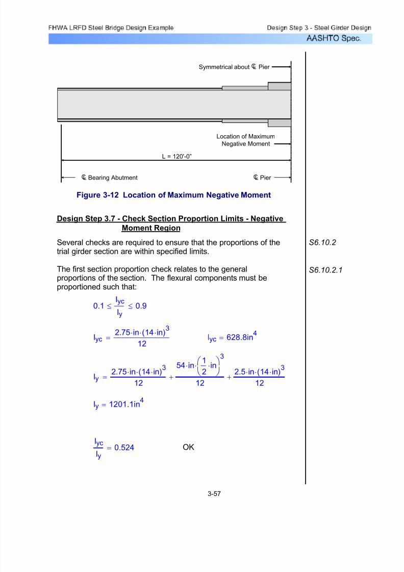
7/29/2019 LRFD steel design.pdf
http://slidepdf.com/reader/full/lrfd-steel-designpdf 168/646
L = 120'-0”
Location of Maximum
Negative Moment
Symmetrical about L Pier C
L Pier CL Bearing AbutmentC
Figure 3-12 Location of Maximum Negative Moment
Design Step 3.7 - Check Section Proportion Limits - Negative
Moment Region
Several checks are required to ensure that the proportions of thetrial girder section are within specified limits.
The first section proportion check relates to the generalproportions of the section. The flexural components must beproportioned such that:
S6.10.2
S6.10.2.1
0.1 Iyc
Iy≤ 0.9≤
Iyc2.75 in⋅ 14 in⋅( )
3⋅12
= Iyc 628.8in4
=
Iy2.75 in⋅ 14 in⋅( )
3⋅12
54 in⋅1
2in⋅⎛
⎝ ⎞ ⎠
3
⋅
12+
2.5 in⋅ 14 in⋅( )3
⋅12
+=
Iy 1201.1in4=
Iyc
Iy0.524= OK
3-57

7/29/2019 LRFD steel design.pdf
http://slidepdf.com/reader/full/lrfd-steel-designpdf 169/646
OK2 Dc⋅
tw200≤and
2 Dc⋅
tw6.77
E
f c⋅≤
6.77
E
f c⋅ 165.0=
2 Dc⋅
tw119.7=
f c 48.84 ksi⋅=
S6.4.1E 29000ksi=
(see Figure 3-4)tw1
2in=
Dc 29.92in=
(see Figure 3-4 and Table 3-5)
Dc 32.668 in⋅ 2.75 in⋅−=
Dc for Negative Flexure
At sections in negative flexure, using Dc of the
composite section consisting of the steel section plusthe longitudinal reinforcement, as described in
C6.10.3.1.4a, removes the dependency of Dc on theapplied loading, which greatly simplifies subsequentload rating calculations.
C6.10.3.1.4a At sections in negative flexure, using Dc of the compositesection consisting of the steel section plus thelongitudinal reinforcement is conservative.
2 Dc
⋅
tw6.77 E
f c⋅≤ 200≤
S6.10.2.2 The second section proportion check relates to the webslenderness. For a section without longitudinal stiffeners, the webmust be proportioned such that:
3-58

7/29/2019 LRFD steel design.pdf
http://slidepdf.com/reader/full/lrfd-steel-designpdf 170/646
OKbt
2 tt⋅2.8=
(see Figure 3-4)tt 2.5in=
(see Figure 3-4)bt 14in=
bt
2 tt⋅12.0≤
S6.10.2.3In addition to the compression flange check, the tension flangeson fabricated I-sections must be proportioned such that:
C6.10.2.3 According to C6.10.2.3, it is preferable for the flange width to begreater than or equal to 0.4Dc. In this case, the flange width isgreater than both 0.3Dc and 0.4Dc, so this requirement is clearlysatisfied.
OKbf 0.3 Dc⋅≥
0.3 Dc⋅ 8.98in=
Dc 29.92in=
(see Figure 3-4)bf 14in=
bf 0.3 Dc⋅≥
S6.10.2.3The third section proportion check relates to the flangeproportions. The compression flanges on fabricated I-sectionsmust be proportioned such that:
3-59

7/29/2019 LRFD steel design.pdf
http://slidepdf.com/reader/full/lrfd-steel-designpdf 171/646
Fyrt 60ksi=
For the longitudinal reinforcing steel in the top layer of the slab at the pier:
Pc 1925K=Pc Fyc bc⋅ tc⋅=
tc 2.75in=bc 14in=Fyc 50ksi=
For the compression flange:
Pw 1350K=Pw Fyw Dw⋅ tw⋅=
tw 0.50in=Dw 54in=Fyw 50.0ksi=
For the web:
Pt 1750K=Pt Fyt bt⋅ tt⋅=
tt 2.50in=bt 14in=Fyt 50ksi=
SAppendix A6.1For the tension flange:
Figure 3-13 Computation of Plastic Moment Capacity for
Negative Bending Sections
tt
bt
tw
bc
Dw
tc
Y
PlasticNeutral Axis
Prb
Pt
Pw
Pc
Art
Arb
Prt
S6.10.3.1.3For composite sections, the plastic moment, Mp, is calculated as
the first moment of plastic forces about the plastic neutral axis.
Design Step 3.8 - Compute Plastic Moment Capacity - Negative
Moment Region
3-60

7/29/2019 LRFD steel design.pdf
http://slidepdf.com/reader/full/lrfd-steel-designpdf 172/646
S6.10.4.1.1
The next step in the design process is to determine if the section iscompact or noncompact. This, in turn, will determine which formulaeshould be used to compute the flexural capacity of the girder.
Where the specified minimum yield strength does not exceed 70.0
ksi, and the girder has a constant depth, and the girder does nothave longitudinal stiffeners or holes in the tension flange, then thefirst step is to check the compact-section web slendernessprovisions, as follows:
Design Step 3.9 - Determine if Section is Compact or
Noncompact - Negative Moment Region
Since it will be shown in the next design step that this section is
noncompact, the plastic moment is not used to compute theflexural resistance and therefore does not need to be computed.
Y 15.17 in=
STable A6.1-2 YD
2
⎛ ⎝
⎞ ⎠
Pc Pt− Prt− Prb−
Pw1+
⎛
⎝
⎞
⎠⋅=
Therefore the plastic neutral axis is located within the web.
Prb Prt+ 766K=Pc Pw+ Pt+ 5025K=
Pt Prb+ Prt+ 2516K=Pc Pw+ 3275K=
SAppendix A6.1Check the location of the plastic neutral axis, as follows:
Prb 383K=Prb Fyrb Arb⋅=
Arb 6.39in2= Arb 0.31 in
2⋅103in
5in
⎛ ⎝
⎞ ⎠
⋅=
Fyrb 60ksi=
For the longitudinal reinforcing steel in the bottom layer of the slab at the pier:
Prt 383K=Prt Fyrt Art⋅=
Art 6.39in2= Art 0.31 in
2⋅103 in⋅
5in
⎛ ⎝
⎞ ⎠
⋅=
3-61

7/29/2019 LRFD steel design.pdf
http://slidepdf.com/reader/full/lrfd-steel-designpdf 173/646
It 628.9in4
=Ittc bc
3⋅
12
Dc
3tw
3⋅
12+=
tc 2.75in=bc 14.0in=
Dc
39.97in=Dc 29.92in=
The term, r t, is defined as the radius of gyration of a notionalsection comprised of the compression flange of the steel sectionplus one-third of the depth of the web in compression taken aboutthe vertical axis.
Based on previous computations,
S6.10.4.1.9Lb Lp≤ 1.76 r t⋅E
Fyc⋅=Lb Lp≤ 1.76 r t⋅
E
Fyc⋅=
Therefore, the investigation proceeds with the noncompact section
compression-flange bracing provisions of S6.10.4.1.9.
bf
2 tf ⋅2.5=
tf 2.75in=bf 14.0in=
bf
2 tf ⋅12.0≤ S6.10.4.1.4
Therefore, the web does not qualify as compact. Since this is not acomposite section in positive flexure, the investigation proceedswith the noncompact section compression-flange slenderness
provisions of S6.10.4.1.4.
3.76E
Fyc⋅ 90.6=
2 Dcp⋅
tw155.3=
Dcp 38.83in=Dcp Dw Y−=Since the plastic neutral axis is located within the web,
2 Dcp⋅
tw3.76
E
Fyc⋅≤
S6.10.4.1.2
3-62

7/29/2019 LRFD steel design.pdf
http://slidepdf.com/reader/full/lrfd-steel-designpdf 174/646
D
227.00in=D 54.0in=
f c 48.84ksi=Dc 29.92in=
for sections where Dc is greater than D/2λb 4.64=
S6.10.4.3.2 The load-shedding factor, Rb, is computed as follows:
S6.10.4.2.4aFn Rb Rh⋅ Fcr ⋅=
S6.10.4.2.5aThe nominal flexural resistance of the compression flange, in termsof stress, is determined from the following equation:
S6.10.4.2.5 Since the section was determined to be noncompact and based onthe computations in the previous design step, the nominal flexuralresistance is computed based upon lateral torsional buckling.
Design Step 3.10 - Design for Flexure - Strength Limit State -
Negative Moment Region
Noncompact Sections
Based on the previous computations, it wasdetermined that the girder section at the pier isnoncompact. Several steps could be taken to makethis a compact section, such as increasing the webthickness or possibly modifying the flange thicknessesto decrease the value Dcp. However, such revisionsmay not be economical.
Therefore, the investigation proceeds with the composite section
lateral torsional buckling provisions of S6.10.4.2.5 .
Lb 20.0ft=
Lp 13.43ft=Lp 1.76 r t⋅E
Fyc⋅=
r t 3.80in=r t
It
At=
At 43.5in2= At tc bc⋅( )
Dc
3tw⋅
⎛ ⎝
⎞ ⎠
+=
3-63

7/29/2019 LRFD steel design.pdf
http://slidepdf.com/reader/full/lrfd-steel-designpdf 175/646
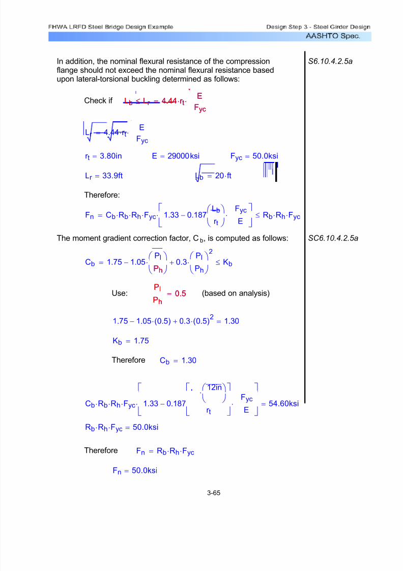
7/29/2019 LRFD steel design.pdf
http://slidepdf.com/reader/full/lrfd-steel-designpdf 176/646
Fn 50.0ksi=
Fn Rb Rh⋅ Fyc⋅=Therefore
Rb Rh⋅ Fyc⋅ 50.0ksi=
Cb Rb⋅ Rh⋅ Fyc⋅ 1.33 0.187
Lb12in
ft
⎛
⎝
⎞
⎠
⋅
r t
⎡
⎣
⎤
⎦FycE
⋅−
⎡
⎣
⎤
⎦⋅ 54.60ksi=
Cb 1.30=Therefore
Kb 1.75=
1.75 1.05 0.5( )⋅− 0.3 0.5( )2⋅+ 1.30=
(based on analysis)Pl
Ph
0.5=Pl
Ph
0.5=Use:
Cb 1.75 1.05Pl
Ph
⎛
⎝
⎞
⎠⋅− 0.3
Pl
Ph
⎛
⎝
⎞
⎠
2
⋅+ Kb≤=Ph
SC6.10.4.2.5aThe moment gradient correction factor, Cb, is computed as follows:
Fn Cb Rb⋅ Rh⋅ Fyc⋅ 1.33 0.187Lb
r t
⎛
⎝
⎞
⎠
Fyc
E⋅−
⎡
⎣
⎤
⎦⋅ Rb Rh⋅ Fyc⋅≤=
Therefore:
Lb 20 ft⋅=Lr 33.9ft=
Fyc 50.0ksi=E 29000ksi=r t 3.80in=
Lr 4.44 r t⋅E
Fyc⋅=
Lb Lr ≤ 4.44 r t⋅ EFyc
⋅=Lb Lr ≤ 4.44 r t⋅ EFyc
⋅=Check if
S6.10.4.2.5aIn addition, the nominal flexural resistance of the compressionflange should not exceed the nominal flexural resistance basedupon lateral-torsional buckling determined as follows:
3-65
7/29/2019 LRFD steel design.pdf
http://slidepdf.com/reader/full/lrfd-steel-designpdf 177/646
Fr 50.00ksi= OK
For the tension flange, the nominal flexural resistance, in terms of stress, is determined as follows:
S6.10.4.2.5b
Fn Rb Rh⋅ Fyt⋅=
where: Rb 1.0= S6.10.4.3.2b
Rh 1.0=
Fyt 50.0ksi=
Fn 50.0ksi=
The factored flexural resistance, Fr , is computed as follows: S6.10.4
φf 1.00= S6.5.4.2
Fr φf Fn⋅=
Fr 50.0ksi=
The factored flexural resistance, Fr , is computed as follows: S6.10.4
φf 1.00= S6.5.4.2
Fr φf
Fn⋅=
Fr 50.0ksi=
The negative flexural resistance at this design section is checked asfollows:
S1.3.2.1
Σηi γ i⋅ Qi⋅ Rr ≤
or in this case:
Σηi γ i⋅ Fi⋅ Fr ≤
For this design example,
η i 1.00=
As computed in Design Step 3.6, the factored Strength I LimitState stress for the compression flange is as follows:
Σγi Fi⋅ 48.84ksi=Σγi Fi⋅ 48.84ksi=
Therefore Σηi γ i⋅ Fi⋅ 48.84 ksi⋅=Σηi γ i⋅ Fi⋅ 48.84 ksi⋅=
3-66

7/29/2019 LRFD steel design.pdf
http://slidepdf.com/reader/full/lrfd-steel-designpdf 178/646
1.10E k⋅Fyw
⋅ 59.2=
D
tw108.0= S6.10.7.3.3a
S6.10.7.3.3ak 5.0=
Vn C Vp⋅= Vp
S6.10.7.2
S6.10.7 Shear must be checked at each section of the girder. For thisdesign example, shear is maximum at the pier.
The first step in the design for shear is to check if the web must bestiffened. The nominal shear resistance of unstiffened webs of hybrid and homogeneous girders is:
Design Step 3.11 - Design for Shear - Negative Moment Region
Therefore, the girder design section at the pier satisfies theflexural resistance requirements for both the compression flangeand the tension flange.
OKFr 50.0ksi=
Σηi γ i⋅ Fi⋅ 44.99 ksi⋅=Σηi γ i⋅ Fi⋅ 44.99 ksi⋅=Therefore
Σγi Fi⋅ 44.99ksi=Σγi Fi⋅ 44.99ksi=
As computed in Design Step 3.6, the factored Strength I LimitState stress for the tension flange is as follows:
η i 1.00=
For this design example,
Σηi γ i⋅ Fi⋅ Fr ≤
or in this case:
Σηi γ i⋅ Qi⋅ Rr ≤
S1.3.2.1The negative flexural resistance at this design section is checkedas follows:
3-67

7/29/2019 LRFD steel design.pdf
http://slidepdf.com/reader/full/lrfd-steel-designpdf 179/646
Σγ i Vi⋅ 423.5 K⋅=Σγ i Vi⋅ 423.5 K⋅=
As computed in Design Step 3.6, the factored Strength I LimitState shear is as follows:
η i 1.00=
For this design example,Σηi γ i⋅ Vi⋅ Vr ≤
or in this case:
Σηi γ i⋅ Qi⋅ Rr ≤
S1.3.2.1The shear resistance at this design section is checked as follows:
Vr 295.9K=
Vr φv Vn⋅=
S6.5.4.2 φv 1.00=
S6.10.7.1The factored shear resistance, Vr , is computed as follows:
Vn 295.9K=
Vn C Vp⋅=
Vp 783.0K=
S6.10.7.3.3a&c Vp 0.58 Fyw⋅ D⋅ tw⋅=
tw 0.5in=D 54.0 in=Fyw 50.0ksi=
C 0.378=
C1.52
D
tw
⎛ ⎝
⎞ ⎠
2
E k⋅Fyw
⎛ ⎝
⎞ ⎠
⋅=
D
tw1.38
E k⋅Fyw⋅≥Therefore,
1.38E k⋅Fyw
⋅ 74.3=
3-68
7/29/2019 LRFD steel design.pdf
http://slidepdf.com/reader/full/lrfd-steel-designpdf 180/646
D
tw108.0=
tw 0.5in=D 54.0in=
D
tw150≥
S6.10.7.3.2 First, handling requirements of the web are checked. For webpanels without longitudinal stiffeners, transverse stiffeners must beused if:
Stiffener Spacing
The spacing of the transverse intermediate stiffenersis determined such that it satisfies all spacing
requirement in S6.10.7 and such that the shear resistance of the stiffened web is sufficient to resist theapplied factored shear.
S6.10.7.1For this design example, transverse intermediate stiffeners are usedand longitudinal stiffeners are not used. The transverseintermediate stiffener spacing in this design example is 80 inches.Therefore, the spacing of the transverse intermediate stiffenersdoes not exceed 3D. Therefore, the design section can be
considered stiffened and the provisions of S6.10.7.3 apply.
Nominally Stiffened Webs
As previously explained, a "nominally stiffened" web(approximately 1/16 inch thinner than "unstiffened") willgenerally provide the least cost alternative or veryclose to it. However, for web depths of approximately50 inches or less, unstiffened webs may be moreeconomical.
Since the shear resistance of an unstiffened web is less than theactual design shear, the web must be stiffened.
Vr 295.9K=
Σηi γ i⋅ Vi⋅ 423.5 K⋅=Σηi γ i⋅ Vi⋅ 423.5 K⋅=Therefore
3-69

7/29/2019 LRFD steel design.pdf
http://slidepdf.com/reader/full/lrfd-steel-designpdf 181/646
S6.10.7.3.3ak 7.3=k 55
do
D
⎛ ⎝
⎞ ⎠
2+=
Vn R Vp⋅ C0.87 1 C−( )⋅
1do
D
⎛ ⎝
⎞ ⎠
2
+
+⎡⎢
⎣
⎤⎥
⎦
⋅ C Vp⋅≥= R Vp⋅ C0.87 1 C−( )⋅
1do
D
⎛ ⎝
⎞ ⎠
2
+
+⎡⎢
⎣
⎤⎥
⎦
⋅ C Vp⋅≥
f u 0.75 φf ⋅ Fy⋅≥Therefore,
0.75 φf ⋅ Fy⋅ 37.5ksi=
(see Table 3-12)f u 48.84 ksi⋅=
The term, f u, is the flexural stress in the compression or tensionflange due to the factored loading, whichever flange has themaximum ratio of f u to Fr in the panel under consideration.
f u 0.75 φf ⋅ Fy⋅≤Check if
S6.10.7.3.3bThe nominal shear resistance of interior web panels of noncompact
sections which are considered stiffened, as per S6.10.7.1, is asfollows:
This handling requirement for transverse stiffeners need only be
enforced in regions where transverse stiffeners are no longer required for shear and where the web slenderness ratio exceeds150. Therefore, this requirement must typically be applied only in thecentral regions of the spans of relatively deep girders, where theshear is low.
OKdo 80.0 in⋅=Use
D260
D
tw
⎛ ⎝
⎞ ⎠
⎡
⎣
⎤
⎦
2
⋅ 313.0in=
do D260
Dtw
⎛ ⎝
⎞ ⎠
⎡
⎣
⎤
⎦
2
⋅≤
S6.10.7.3.2 Another handling requirement is that the spacing of transversestiffeners, do, must satisfy the following:
3-70

7/29/2019 LRFD steel design.pdf
http://slidepdf.com/reader/full/lrfd-steel-designpdf 182/646
Vn 430.7K=
Vn max R Vp⋅ C0.87 1 C−( )⋅
1do
D
⎛ ⎝
⎞ ⎠
2
+
+⎡
⎢
⎣
⎤
⎥
⎦
⋅ C Vp⋅,⎡
⎢
⎣
⎤
⎥
⎦
=
C Vp⋅ 430.7K=
R Vp⋅ C0.87 1 C−( )⋅
1do
D
⎛ ⎝
⎞ ⎠
2
+
+⎡
⎢
⎣
⎤
⎥
⎦
⋅ 383.7K=
Vp 783.0K=
S6.10.7.3.3a&c Vp 0.58 Fyw⋅ D⋅ tw⋅=
R 0.637=
R 0.6 0.4Fr f u−
Fr 0.75φf Fy⋅−
⎛
⎝
⎞
⎠⋅+
⎡
⎣
⎤
⎦=
S6.10.7.3.3bThe reduction factor applied to the factored shear, R, is computedas follows:
C 0.550=
C1.52
D
tw
⎛
⎝
⎞
⎠
2
E k⋅Fyw
⎛ ⎝
⎞ ⎠
⋅=
D
tw1.38
E k⋅Fyw
⋅≥Therefore,
1.38E k⋅Fyw
⋅ 89.7=
1.10E k⋅
Fyw⋅ 71.5=
D
tw108.0= S6.10.7.3.3a
3-71
7/29/2019 LRFD steel design.pdf
http://slidepdf.com/reader/full/lrfd-steel-designpdf 183/646
S6.10.8.1.1In this design example, it is assumed that the transverseintermediate stiffeners consist of plates welded to one side of the
web. The required interface between the transverse intermediatestiffeners and the top and bottom flanges is described in
S6.10.8.1.1.
The transverse intermediate stiffener configuration is assumed tobe as presented in the following figure.
S6.10.8.1The girder in this design example has transverse intermediatestiffeners. Transverse intermediate stiffeners are used toincrease the shear resistance of the girder. The shear resistancecomputations shown in the previous design step were based on astiffener spacing of 80 inches.
Design Step 3.12 - Design Transverse Intermediate Stiffeners -
Negative Moment Region
Therefore, the girder design section at the pier satisfies the shear resistance requirements for the web.
OKVr 430.7K=
Σηi γ i⋅ Vi⋅ 423.5 K⋅=Σηi γ i⋅ Vi⋅ 423.5 K⋅=
As previously computed, for this design example:
Vr 430.7K=Vr φv Vn⋅=
S6.5.4.2 φv 1.00=
S6.10.7.1The factored shear resistance, Vr , is computed as follows:
3-72
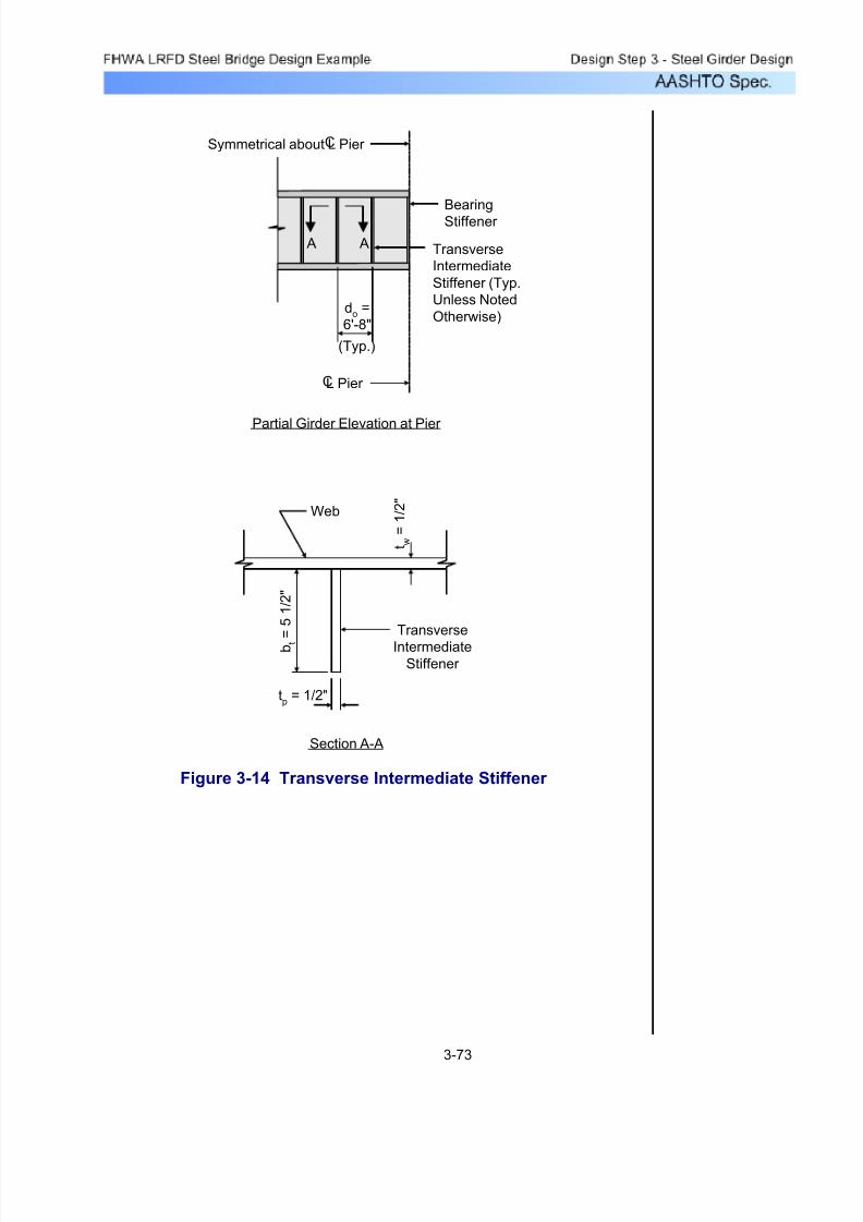
7/29/2019 LRFD steel design.pdf
http://slidepdf.com/reader/full/lrfd-steel-designpdf 184/646
do
=
6'-8"
A A
Partial Girder Elevation at Pier
Section A-A
t w = 1 / 2 "
b t = 5 1 / 2 "
tp
= 1/2"
Transverse
IntermediateStiffener
Web
(Typ.)
Bearing
Stiffener
Transverse
Intermediate
Stiffener (Typ.
Unless Noted
Otherwise)
Symmetrical about L Pier C
L Pier C
Figure 3-14 Transverse Intermediate Stiffener
3-73

7/29/2019 LRFD steel design.pdf
http://slidepdf.com/reader/full/lrfd-steel-designpdf 185/646
16.0 tp⋅ bt≥ 0.25 bf ⋅≥ OK
The second specification check is for the moment of inertia of thetransverse intermediate stiffener. This requirement is intended toensure sufficient rigidity. The moment of inertia of any transverse
stiffener must satisfy the following:
S6.10.8.1.3
It do tw3
⋅ J⋅≥
do 80.0in= tw 0.50in= D 54.0 in=
J 2.5D
do
⎛ ⎝
⎞ ⎠
2
⋅ 2.0− 0.5≥=
2.5D
do
⎛ ⎝
⎞ ⎠
2
⋅ 2.0− 0.9−=
Therefore, J 0.5=
Therefore, do tw3
⋅ J⋅ 5.0in4
=
Ittp bt
3⋅
3= It 27.7in
4=
Therefore, It do tw3⋅ J⋅≥ OK
The first specification check is for the projecting width of thetransverse intermediate stiffener. The width, bt, of each projectingstiffener element must satisfy the following:
S6.10.8.1.2
bt 2.0
d
30.0+≥ and 16.0 tp⋅ bt≥ 0.25bf ≥
bt 5.5in=
d 59.25= in
tp 0.50 in⋅=
bf 14.0in=
bt 5.5in= 2.0d
30.0+ 3.98= in
Therefore, bt 2.0 d30.0
+≥ OK
16.0 tp⋅ 8.0in=
0.25 bf ⋅ 3.5in=
Therefore,
3-74
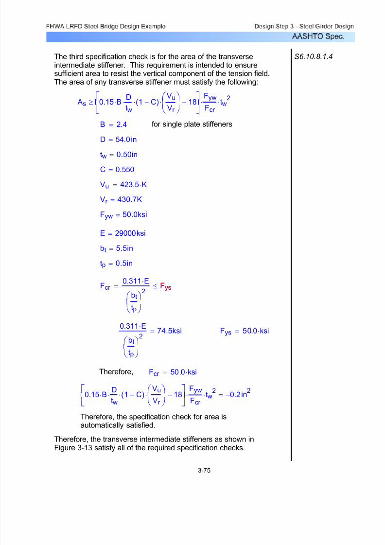
7/29/2019 LRFD steel design.pdf
http://slidepdf.com/reader/full/lrfd-steel-designpdf 186/646
Therefore, the transverse intermediate stiffeners as shown inFigure 3-13 satisfy all of the required specification checks.
Therefore, the specification check for area isautomatically satisfied.
0.15 B⋅D
tw⋅ 1 C−( )⋅
Vu
Vr
⎛
⎝
⎞
⎠⋅ 18−
⎡
⎣
⎤
⎦
Fyw
Fcr ⋅ tw
2⋅ 0.2− in2=
Fcr 50.0 ksi⋅=Therefore,
Fys 50.0 ksi⋅=0.311 E⋅
bt
tp
⎛
⎝
⎞
⎠
274.5ksi=
Fcr 0.311 E⋅
bt
tp
⎛
⎝
⎞
⎠
2 Fys≤= Fys
tp 0.5in=
bt 5.5in=
E 29000ksi=
Fyw 50.0ksi=
Vr 430.7K=
Vu 423.5 K⋅=
C 0.550=
tw 0.50in=
D 54.0in=
for single plate stiffenersB 2.4=
As 0.15 B⋅ D
tw⋅ 1 C−( )⋅ Vu
Vr
⎛ ⎝
⎞ ⎠
⋅ 18−⎡⎣
⎤⎦
Fyw
Fcr ⋅ tw
2⋅≥
S6.10.8.1.4The third specification check is for the area of the transverseintermediate stiffener. This requirement is intended to ensuresufficient area to resist the vertical component of the tension field.The area of any transverse stiffener must satisfy the following:
3-75
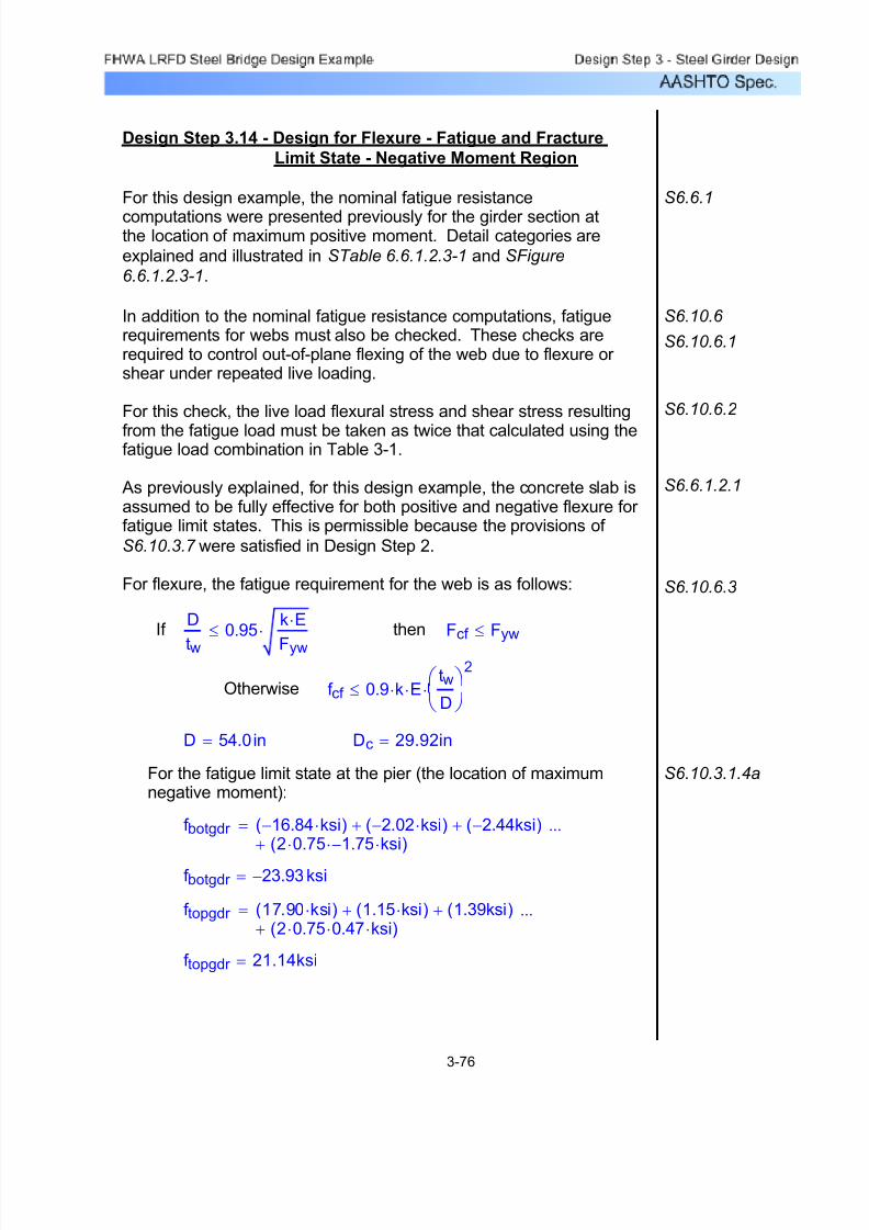
7/29/2019 LRFD steel design.pdf
http://slidepdf.com/reader/full/lrfd-steel-designpdf 187/646
f topgdr 21.14ksi=
f topgdr 17.90 ksi⋅( ) 1.15 ksi⋅( )+ 1.39ksi( )+2 0.75⋅ 0.47⋅ ksi⋅( )+
...=
f botgdr 23.93− ksi=
f botgdr 16.84− ksi⋅( ) 2.02− ksi⋅( )+ 2.44− ksi( )+2 0.75⋅ 1.75−⋅ ksi⋅( )+
...=
S6.10.3.1.4aFor the fatigue limit state at the pier (the location of maximumnegative moment):
Dc 29.92in=D 54.0in=
f cf 0.9 k⋅ E⋅tw
D
⎛ ⎝
⎞ ⎠
2
⋅≤Otherwise
Fcf Fyw≤thenD
tw
0.95k E⋅
Fyw
⋅≤If
S6.10.6.3
S6.6.1.2.1
S6.10.6.2
S6.10.6.1
S6.10.6 In addition to the nominal fatigue resistance computations, fatiguerequirements for webs must also be checked. These checks arerequired to control out-of-plane flexing of the web due to flexure or shear under repeated live loading.
For this check, the live load flexural stress and shear stress resulting
from the fatigue load must be taken as twice that calculated using thefatigue load combination in Table 3-1.
As previously explained, for this design example, the concrete slab isassumed to be fully effective for both positive and negative flexure for fatigue limit states. This is permissible because the provisions of
S6.10.3.7 were satisfied in Design Step 2.
For flexure, the fatigue requirement for the web is as follows:
S6.6.1For this design example, the nominal fatigue resistance
computations were presented previously for the girder section atthe location of maximum positive moment. Detail categories are
explained and illustrated in STable 6.6.1.2.3-1 and SFigure
6.6.1.2.3-1.
Design Step 3.14 - Design for Flexure - Fatigue and Fracture
Limit State - Negative Moment Region
3-76

7/29/2019 LRFD steel design.pdf
http://slidepdf.com/reader/full/lrfd-steel-designpdf 188/646
OKf cf Fyw≤Therefore,
Fyw 50.0ksi=f cf 23.93− ksi=
f cf 16.84− ksi⋅( ) 2.02− ksi⋅( )+ 2.44− ksi( )+2 0.75⋅ 1.75−⋅ ksi⋅( )+
...=
Based on the unfactored stress values in Table 3-12:
D
tw0.95
k E⋅Fyw
⋅≤Therefore,
0.95 k E⋅Fyw⋅ 129.1=D
tw108.0=
k 31.9=k max 9.0D
Dc
⎛ ⎝
⎞ ⎠
2
⋅ 7.2,⎡
⎣
⎤
⎦=
9.0D
Dc
⎛ ⎝
⎞ ⎠
2
⋅ 31.9=k 9.0D
Dc
⎛ ⎝
⎞ ⎠
2
⋅ 7.2≥=
Dc 28.70in=
Dc Depthcomp tbotfl−=
Depthcomp 31.45in=
C6.10.3.1.4aDepthcompf botgdr −
f topgdr f botgdr −Depthgdr ⋅=
Depthgdr 59.25in=
Depthgdr ttopfl Dweb+ tbotfl+=(see Figure 3-4)tbotfl 2.75in=
(see Figure 3-4)Dweb 54in=
(see Figure 3-4)ttopfl 2.50in=
3-77

7/29/2019 LRFD steel design.pdf
http://slidepdf.com/reader/full/lrfd-steel-designpdf 189/646
S6.10.5.1The web must satisfy SEquation 6.10.3.2.2-1, using theappropriate value of the depth of the web in compression in theelastic range, Dc.
C6.10.5.1This check will not control for composite noncompact sections
under the load combinations given in STable 3.4.1-1. Althougha web bend buckling check is also required in regions of positiveflexure at the service limit state according to the currentspecification language, it is unlikely that such a check wouldcontrol in these regions for composite girders without
longitudinal stiffeners since Dc is relatively small for such girdersin these regions.
S6.10.5 The girder must be checked for service limit state control of permanent deflection. This check is intended to preventobjectionable permanent deflections due to expected severe trafficloadings that would impair rideability. Service II Limit State is usedfor this check.
Design Step 3.15 - Design for Flexure - Service Limit State -
Negative Moment Region
Therefore, the fatigue requirements for webs for both flexure andshear are satisfied.
OKvcf 0.58 C⋅ Fyw⋅≤Therefore,
0.58 C⋅ Fyw⋅ 15.95ksi=
Fyw 50.0ksi=C 0.550=
vcf 8.17ksi=vcf Vcf
D tw⋅=
tw 0.50in=D 54.0in=
Vcf 220.7K=
Vcf 114.7 K⋅ 16.4 K⋅+ 19.8 K⋅+ 2 0.75⋅ 46.5⋅ K⋅( )+=
Based on the unfactored shear values in Table 3-13:
vcf 0.58 C⋅ Fyw⋅≤
S6.10.6.4For shear, the fatigue requirement for the web is as follows:
3-78

7/29/2019 LRFD steel design.pdf
http://slidepdf.com/reader/full/lrfd-steel-designpdf 190/646
(see Figure 3-4)tw 0.5in=
k 25.1=k max 9.0D
Dc
⎛ ⎝
⎞ ⎠
2
⋅ 7.2,⎡
⎣
⎤
⎦=
9.0D
Dc
⎛ ⎝
⎞ ⎠
2
⋅ 25.1=
for webs withoutlongitudinal stiffeners
k 9.0D
Dc
⎛ ⎝
⎞ ⎠
2
⋅ 7.2≥=
Dc 32.33in=
Dc Depthcomp tbotfl−=
Depthcomp 35.08in=
Depthcompf botgdr −
f topgdr f botgdr −Depthgdr ⋅=
(see Figure 3-4)Depthgdr 59.25in=
f topgdr 24.12 ksi⋅=
f botgdr 35.01− ksi⋅=
The factored Service II flexural stress was previouslycomputed in Table 3-12 as follows:
D 54.0in=
for webs without longitudinal stiffenersα 1.25=
E 29000ksi=
for which:
f cw0.9 E⋅ α⋅ k⋅
D
tw
⎛ ⎝
⎞ ⎠
2≤ Fyw≤
3-79
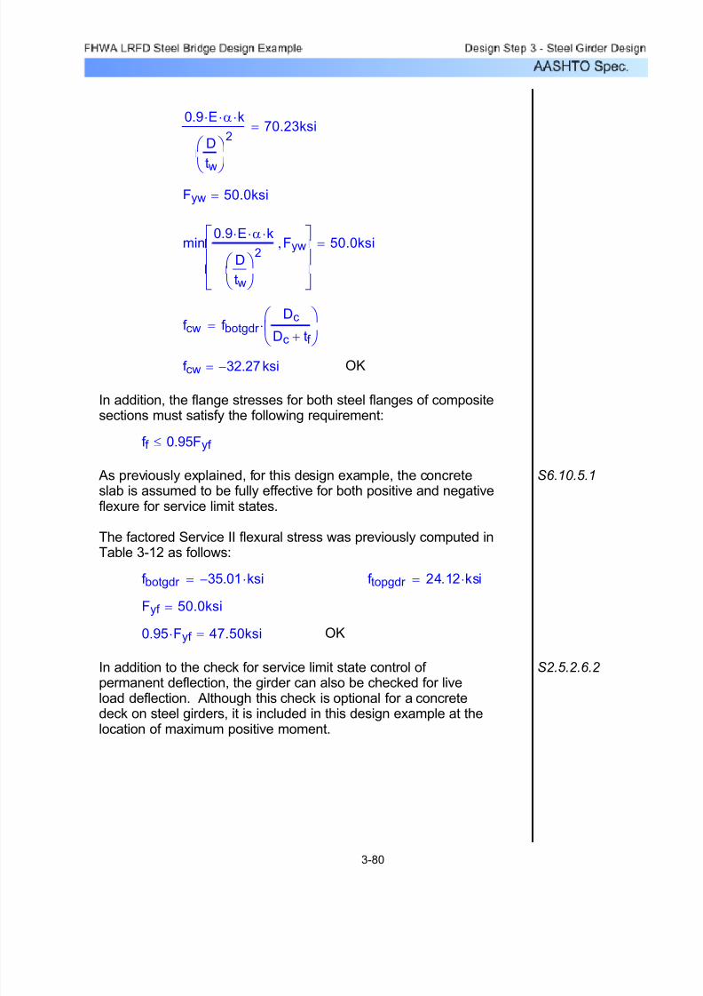
7/29/2019 LRFD steel design.pdf
http://slidepdf.com/reader/full/lrfd-steel-designpdf 191/646
S2.5.2.6.2 In addition to the check for service limit state control of permanent deflection, the girder can also be checked for live
load deflection. Although this check is optional for a concretedeck on steel girders, it is included in this design example at thelocation of maximum positive moment.
OK0.95 Fyf ⋅ 47.50ksi=
Fyf 50.0ksi=
f topgdr 24.12 ksi⋅=f botgdr 35.01− ksi⋅=
S6.10.5.1 As previously explained, for this design example, the concreteslab is assumed to be fully effective for both positive and negativeflexure for service limit states.
The factored Service II flexural stress was previously computed inTable 3-12 as follows:
f f 0.95Fyf ≤
In addition, the flange stresses for both steel flanges of compositesections must satisfy the following requirement:
OKf cw 32.27− ksi=
f cw f botgdr Dc
Dc tf +
⎛
⎝
⎞
⎠⋅=
min0.9 E⋅ α⋅ k⋅
D
tw
⎛ ⎝
⎞ ⎠
2Fyw,
⎡
⎢
⎣
⎤
⎥
⎦
50.0ksi=
Fyw 50.0ksi=
0.9 E⋅ α⋅ k⋅
D
tw
⎛
⎝
⎞
⎠
270.23ksi=
3-80
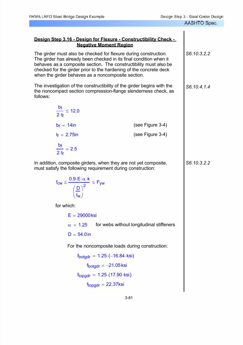
7/29/2019 LRFD steel design.pdf
http://slidepdf.com/reader/full/lrfd-steel-designpdf 192/646
f topgdr 22.37ksi=
f topgdr 1.25 17.90 ksi⋅( )⋅=
f botgdr 21.05− ksi=
f botgdr 1.25 16.84− ksi⋅( )⋅=
For the noncomposite loads during construction:
D 54.0in=
for webs without longitudinal stiffenersα 1.25=
E 29000ksi=
for which:
f cw 0.9 E⋅ α⋅ k⋅D
tw
⎛ ⎝
⎞ ⎠
2≤ Fyw≤
S6.10.3.2.2 In addition, composite girders, when they are not yet composite,must satisfy the following requirement during construction:
bf
2 tf ⋅2.5=
(see Figure 3-4)tf 2.75in=
(see Figure 3-4)bf 14in=
bf
2 tf ⋅12.0≤
S6.10.4.1.4
S6.10.3.2.2 The girder must also be checked for flexure during construction.
The girder has already been checked in its final condition when itbehaves as a composite section. The constructibility must also bechecked for the girder prior to the hardening of the concrete deckwhen the girder behaves as a noncomposite section.
The investigation of the constructibility of the girder begins with thethe noncompact section compression-flange slenderness check, asfollows:
Design Step 3.16 - Design for Flexure - Constructibility Check -
Negative Moment Region
3-81

7/29/2019 LRFD steel design.pdf
http://slidepdf.com/reader/full/lrfd-steel-designpdf 193/646
OKf cw 19.03− ksi=
f cw f botgdr Dc
Dc tf +
⎛
⎝
⎞
⎠⋅=
min0.9 E⋅ α⋅ k⋅
D
tw
⎛ ⎝
⎞ ⎠
2Fyw,
⎡
⎢
⎣
⎤
⎥
⎦
50.0ksi=
Fyw 50.0ksi=
0.9 E⋅ α⋅ k⋅D
tw
⎛ ⎝
⎞ ⎠
2108.83ksi=
(see Figure 3-4)tw 0.5in=
k 38.9=k max 9.0D
Dc
⎛ ⎝
⎞ ⎠
2
⋅ 7.2,⎡
⎣
⎤
⎦=
9.0D
Dc
⎛ ⎝
⎞ ⎠
2
⋅ 38.9=
for webs without
longitudinal stiffeners
k 9.0D
Dc
⎛
⎝
⎞
⎠
2
⋅ 7.2≥=
Dc 25.97in=
Dc Depthcomp tbotfl−=
Depthcomp 28.72in=
C6.10.3.1.4aDepthcompf botgdr −
f topgdr f botgdr −Depthgdr ⋅=
(see Figure 3-4)Depthgdr 59.25in=
3-82
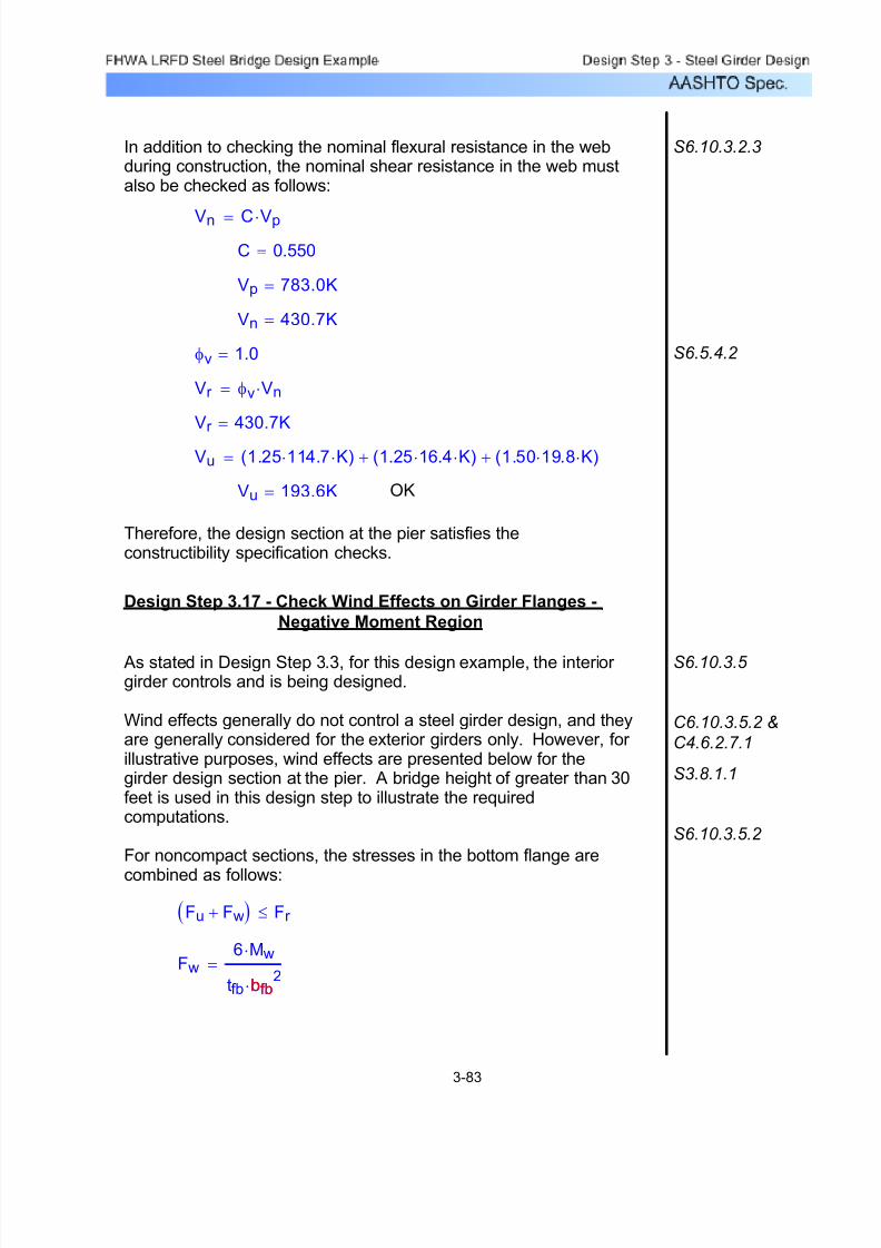
7/29/2019 LRFD steel design.pdf
http://slidepdf.com/reader/full/lrfd-steel-designpdf 194/646
Fw6 Mw⋅
tfb bfb2⋅
=bfb
Fu Fw+( ) Fr ≤
S6.10.3.5.2
S3.8.1.1
C6.10.3.5.2 &
C4.6.2.7.1
S6.10.3.5 As stated in Design Step 3.3, for this design example, the interior girder controls and is being designed.
Wind effects generally do not control a steel girder design, and theyare generally considered for the exterior girders only. However, for illustrative purposes, wind effects are presented below for thegirder design section at the pier. A bridge height of greater than 30feet is used in this design step to illustrate the requiredcomputations.
For noncompact sections, the stresses in the bottom flange are
combined as follows:
Design Step 3.17 - Check Wind Effects on Girder Flanges -
Negative Moment Region
Therefore, the design section at the pier satisfies theconstructibility specification checks.
OKVu 193.6K=
Vu 1.25 114.7⋅ K⋅( ) 1.25 16.4⋅ K⋅( )+ 1.50 19.8⋅ K⋅( )+=
Vr 430.7K=
Vr φv Vn⋅=
S6.5.4.2 φv 1.0=
Vn 430.7K=
Vp 783.0K=
C 0.550=
Vn C Vp⋅=
S6.10.3.2.3In addition to checking the nominal flexural resistance in the webduring construction, the nominal shear resistance in the web mustalso be checked as follows:
3-83

7/29/2019 LRFD steel design.pdf
http://slidepdf.com/reader/full/lrfd-steel-designpdf 195/646
MPHVB 100=
STable3.8.1.2.1-1
PB 0.050 ksf ⋅=
PD PBVDZ
VB
⎛
⎝
⎞
⎠
2
⋅=VB
S3.8.1.2 Assume that the bridge is to be constructed in Pittsburgh,Pennsylvania. The design horizontal wind pressure is computed asfollows:
STable 3.4.1-1 for Strength V Limit Stateγ 0.40=
Strength Limit States for Wind on Structure
For the strength limit state, wind on the structure isconsidered for the Strength III and Strength V LimitStates. For Strength III, the load factor for wind onstructure is 1.40 but live load is not considered. Dueto the magnitude of the live load stresses, Strength IIIwill clearly not control for this design example (and for most designs). Therefore, for this design example, theStrength V Limit State will be investigated.
S1.3 η 1.0=
Wη γ⋅ PD⋅ d⋅
2=
PD
Lb 20.0ft=
MwW Lb
2⋅
10=
W
C4.6.2.7.1Since the deck provides horizontal diaphragm action and sincethere is wind bracing in the superstructure, the maximum windmoment on the loaded flange is determined as follows:
3-84
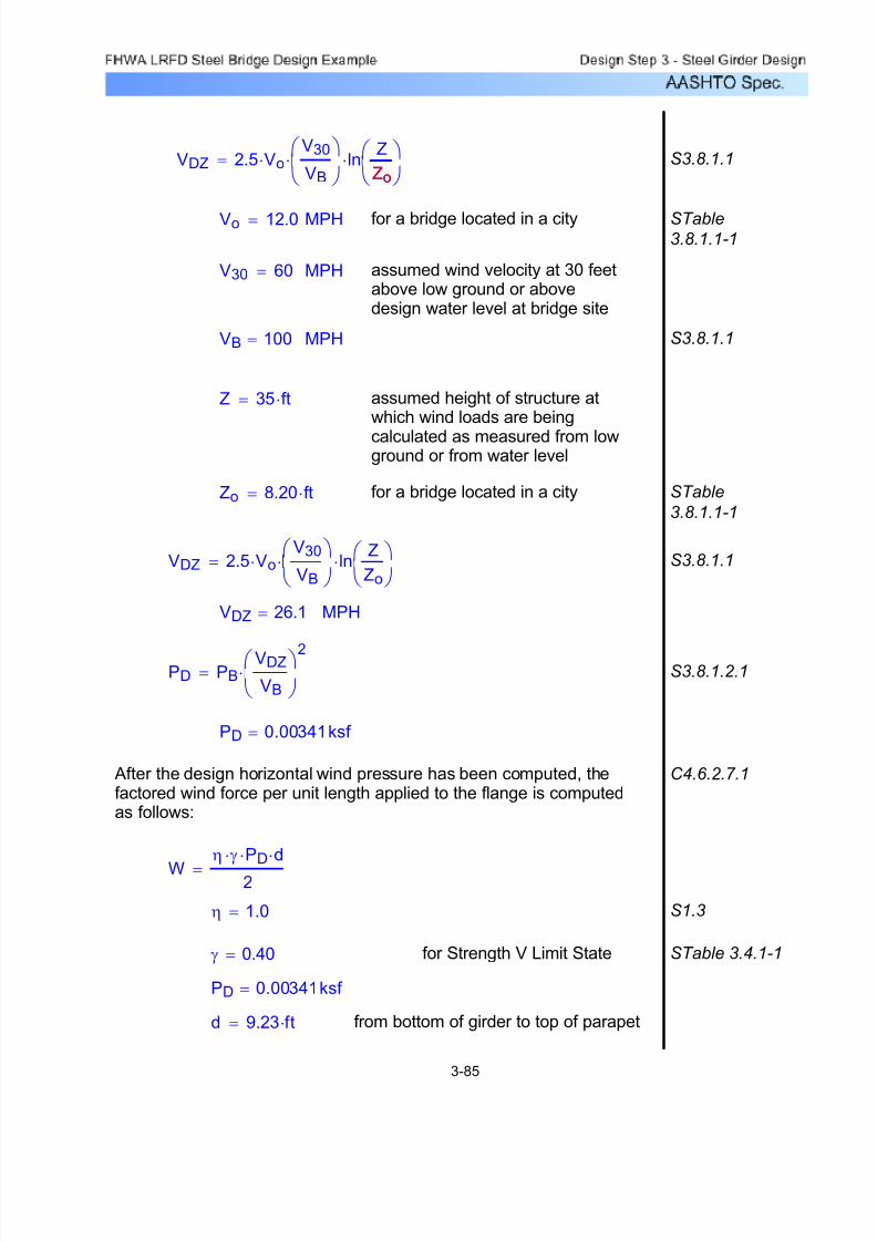
7/29/2019 LRFD steel design.pdf
http://slidepdf.com/reader/full/lrfd-steel-designpdf 196/646
VDZ 2.5 Vo⋅V30
VB
⎛
⎝
⎞
⎠⋅ ln
Z
Zo
⎛ ⎝
⎞ ⎠
⋅= S3.8.1.1
VDZ 26.1= MPH
PD PBVDZ
VB
⎛ ⎝
⎞ ⎠
2⋅= S3.8.1.2.1
PD 0.00341ksf =
After the design horizontal wind pressure has been computed, thefactored wind force per unit length applied to the flange is computedas follows:
C4.6.2.7.1
W
η γ⋅ PD⋅ d⋅
2=
η 1.0= S1.3
γ 0.40= for Strength V Limit State STable 3.4.1-1
PD 0.00341ksf =
d 9.23 ft⋅= from bottom of girder to top of parapet
VDZ 2.5 Vo⋅V30
VB
⎛
⎝
⎞
⎠⋅ ln
Z
Zo
⎛ ⎝
⎞ ⎠
⋅=Zo
S3.8.1.1
Vo 12.0= MPH for a bridge located in a city STable3.8.1.1-1
V30 60= MPH assumed wind velocity at 30 feetabove low ground or abovedesign water level at bridge site
VB 100= MPH S3.8.1.1
Z 35 ft⋅= assumed height of structure atwhich wind loads are being
calculated as measured from lowground or from water level
Zo 8.20 ft⋅= for a bridge located in a city STable
3.8.1.1-1
3-85

7/29/2019 LRFD steel design.pdf
http://slidepdf.com/reader/full/lrfd-steel-designpdf 197/646
The load factor for live load is 1.35 for the Strength V Limit State.However, it is 1.75 for the Strength I Limit State, which we havealready investigated. Therefore, it is clear that wind effects will notcontrol the design of this steel girder. Nevertheless, the followingcomputations are presented simply to demonstrate that wind effectsdo not control this design:
Fw 0.034ksi=
Fw6 Mw⋅
tfb bfb2
⋅=
bfb 14.0 in⋅=
tfb 2.75 in⋅=Mw 0.252K ft⋅=
Fw6 Mw⋅
tfb bfb2
⋅=
bfb
S6.10.3.5.2 Finally, the flexural stress at the edges of the bottom flange due tofactored wind loading is computed as follows:
Mw 0.252K ft⋅=
Lb 20.0ft=
W 0.00630K
ft=
MwW Lb
2⋅
10=
C4.6.2.7.1 Next, the maximum lateral moment in the flange due to the factoredwind loading is computed as follows:
W 0.00630
K
ft=
Wη γ⋅ PD⋅ d⋅
2=
3-86

7/29/2019 LRFD steel design.pdf
http://slidepdf.com/reader/full/lrfd-steel-designpdf 198/646
Fu 1.25 16.84−⋅ ksi( ) 1.25 2.15−⋅ ksi( )+1.50 2.61−⋅ ksi⋅( ) 1.35 12.11−⋅ ksi⋅( )++
...=
Fu 44.00− ksi=
Fw 0.028− ksi⋅=
Fu Fw+ 44.03− ksi=
Fr 50.0ksi=
Therefore: Fu Fw+( ) Fr ≤ OK
Therefore, wind effects do not control the design of this steel girder.
Design Step 3.18 - Draw Schematic of Final Steel Girder Design
Since all of the specification checks were satisfied, the trial girder section presented in Design Step 3.2 is acceptable. If any of thespecification checks were not satisfied or if the design were foundto be overly conservative, then the trial girder section would need tobe revised appropriately, and the specification checks would needto be repeated for the new trial girder section.
The following is a schematic of the final steel girder configuration:
84'-0” 12'-0”
120'-0”
14” x 7/8” Bottom Flange
14” x 1 1/4” Top Flange
14” x 2 3/4”
Bottom Flange
14” x 2 1/2”
Top Flange
L Bearing Abutment L Pier
Symmetrical about L Pier
L Bolted Field Splice
54” x 1/2” Web
C
C
C C
8”
24'-0”
14” x 1 3/8” Bottom Flange
14” x 5/8” Top Flange
6'-8”
5 1/2” x 1/2” TransverseIntermediate Stiffener
(One Side of Web Only -
Interior Side of Fascia Girders)
(Typ. Unless Noted Otherwise)
Bearing Stiffener
(Both Sides of Web)Bearing Stiffener
(Both Sides of Web)
(Typ.)
Figure 3-15 Final Plate Girder Elevation
3-87

7/29/2019 LRFD steel design.pdf
http://slidepdf.com/reader/full/lrfd-steel-designpdf 199/646
For this design example, only the location of maximum positivemoment, the location of maximum negative moment, and the locationof maximum shear were investigated. However, the aboveschematic shows the plate sizes and stiffener spacing throughout theentire length of the girder. Some of the design principles for thisdesign example are presented in "tip boxes."
Design computations for a bolted field splice are presented inDesign Step 4. Design computations and principles for shear connectors, bearing stiffeners, welded connections, andcross-frames are presented in Design Step 5. Design computationsfor an elastomeric bearing pad are presented in Design Step 6.
3-88

7/29/2019 LRFD steel design.pdf
http://slidepdf.com/reader/full/lrfd-steel-designpdf 200/646
Refer to Design Step 1 for introductory information about this designexample. Additional information is presented about the designassumptions, methodology, and criteria for the entire bridge, includingthe splice.
This splice design example is based on AASHTO LRFD Bridge
Design Specifications (through 2002 interims). The design methodspresented throughout the example are meant to be the most widelyused in general bridge engineering practice.
The first design step is to identify the appropriate design criteria. Thisincludes, but is not limited to, defining material properties, identifyingrelevant superstructure information, and determining the splice location.
Design Step 4.1 - Obtain Design Criteria
103Design Step 4.8 - Draw Schematic of Final Bolted FieldSplice Design
77Design Step 4.7 - Design Web Splice
61Design Step 4.6 - Compute Web Splice Design Loads
60Design Step 4.5 - Design Top Flange Splice
31Design Step 4.4 - Design Bottom Flange Splice
6Design Step 4.3 - Compute Flange Splice Design Loads
6Design Step 4.2 - Select Girder Section as Basis for Field Splice Design
1Design Step 4.1 - Obtain Design Criteria
PageTable of Contents
Bolted Field Splice Design ExampleDesign Step 4
4-1

7/29/2019 LRFD steel design.pdf
http://slidepdf.com/reader/full/lrfd-steel-designpdf 201/646
Presented in Figure 4-1 is the final steel girder configuration asdesigned in Design Step 3. Included in Figure 4-1 is the bolted fieldsplice location. This location was determined using the criteriapresented in the narrative below.
84'-0” 12'-0”
120'-0”
14” x 7/8” Bottom Flange
14” x 1 1/4” Top Flange
14” x 2 3/4”Bottom Flange
14” x 2 1/2”Top Flange
L Bearing Abutment L Pier
Symmetrical about L Pier
L Bolted Field Splice
54” x 1/2” Web
C
C
C C
8”
24'-0”
14” x 1 3/8” Bottom Flange
14” x 5/8” Top Flange
Figure 4-1 Plate Girder Elevation
The following units are defined for use in this design example:
K 1000lb= kcf K
ft
3= ksi
K
in
2=
For relatively long girders, field splices are generally required to reducethe girder shipping length. The location of the field splice is generallybased on economy and includes the following considerations:
1.
2.
3.
Field splices are generally located to provide girder segmentlengths that do not exceed the allowable girder shipping length.The allowable girder shipping length is often a function of theshipping route from the fabrication site to the construction site.
The Specifications recommends locating splices near points of dead load contraflexure.
Field splices are generally located where total moment in thegirder is relatively small. This minimizes the required spliceplate thicknesses and the required number of bolts.
S6.13.6.1.4a
4-2
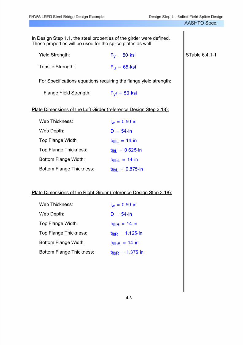
7/29/2019 LRFD steel design.pdf
http://slidepdf.com/reader/full/lrfd-steel-designpdf 202/646
tfltL 0.625 in⋅=
Bottom Flange Width: bflbL 14 in⋅=
Bottom Flange Thickness: tflbL 0.875 in⋅=
Plate Dimensions of the Right Girder (reference Design Step 3.18):
Web Thickness: tw 0.50 in⋅=
Web Depth: D 54 in⋅=
Top Flange Width: bfltR 14 in⋅=
Top Flange Thickness: tfltR 1.125 in⋅=
Bottom Flange Width: bflbR 14 in⋅=
Bottom Flange Thickness: tflbR 1.375 in⋅=
In Design Step 1.1, the steel properties of the girder were defined.These properties will be used for the splice plates as well.
Yield Strength: Fy 50 ksi⋅= STable 6.4.1-1
Tensile Strength: Fu 65 ksi⋅=
For Specifications equations requiring the flange yield strength:
Flange Yield Strength: Fyf 50 ksi⋅=
Plate Dimensions of the Left Girder (reference Design Step 3.18):
Web Thickness: tw 0.50 in⋅=
Web Depth: D 54 in⋅=
Top Flange Width: bfltL 14 in⋅=
Top Flange Thickness:
4-3

7/29/2019 LRFD steel design.pdf
http://slidepdf.com/reader/full/lrfd-steel-designpdf 203/646
Adeckreinfbot 6.386in2=
Adeckreinfbot 0.31 in2⋅( ) Weff
5 in⋅⋅=
For the bottom steel:
Adeckreinftop 6.386in2=
Adeckreinftop 0.31 in2⋅( ) Weff
5 in⋅⋅=
For the top steel:
Based on the concrete deck design example and as illustrated inFigure 2-18, the area of longitudinal deck reinforcing steel in thenegative moment region is computed as follows:
Weff 103 in⋅=Effective Flange Width:
dhaunch 3.5 in⋅=Haunch Depth (measuredfrom top of web):
n 8=Modular Ratio:
tseff 8 in⋅=Effective Slab Thickness:
Concrete Deck Properties (reference Design Step 3.3):
S6.4.3.1Fubolt 120 ksi⋅=Bolt Tensile Strength:
S6.8.3dhole 1.0 in⋅=Bolt Hole Diameter:(for design purposes)
S6.13.2.5dbolt 0.875 in⋅=Bolt Diameter:
Splice Bolt Properties:
4-4

7/29/2019 LRFD steel design.pdf
http://slidepdf.com/reader/full/lrfd-steel-designpdf 204/646
φbs 0.80=Block shear:
φs 0.80= A325 and A490 bolts in shear:
φbb 0.80=Bolts bearing on material:
φy 0.95=Tension, yielding in gross section:
φu 0.80=Tension, fracture in net section:
φc 0.90= Axial Compression:
φv 1.0=Shear:
Flexure: φf 1.0=
S6.5.4.2Resistance Factors:
4-5

7/29/2019 LRFD steel design.pdf
http://slidepdf.com/reader/full/lrfd-steel-designpdf 205/646
MNFLL 284.0− K⋅ ft⋅=Fatigue Negative:
MPFLL 394.3 K⋅ ft⋅=Fatigue Positive:
MNLL 953.3− K⋅ ft⋅=HL-93 Negative:
MPLL 1307.8 K⋅ ft⋅=HL-93 Positive:
Live Loads:
MFWS 18.8 K⋅ ft⋅=Future Wearing Surface:
MCDL 15.5 K⋅ ft⋅=Composite:
MNDL 51.8− K⋅ ft⋅=Noncomposite:
Dead Loads:
MomentsLoads
Based on the properties defined in Design Step 3 (Steel Girder Design), any number of commercially available software programscan be used to obtain the design dead and live loads at the splice.For this design example, the AASHTO Opis software was used. Asummary of the unfactored moments at the splice from the initial trialof the girder design are listed below. The live loads include impactand distribution factors.
Girder Moments at the Splice Location:
Design Step 4.3 - Compute Flange Splice Design Loads
S6.13.6.1.1Design Step 4.2 - Select Girder Section as Basis for Field
Splice Design
Where a section changes at a splice, the smaller of the two
connected sections shall be used in the design. Therefore, thebolted field splice will be designed based on the left adjacent girder section properties. This will be referred to as the Left Girder throughout the calculations. The girder located to the right of thebolted field splice will be designated the Right Girder.
4-6
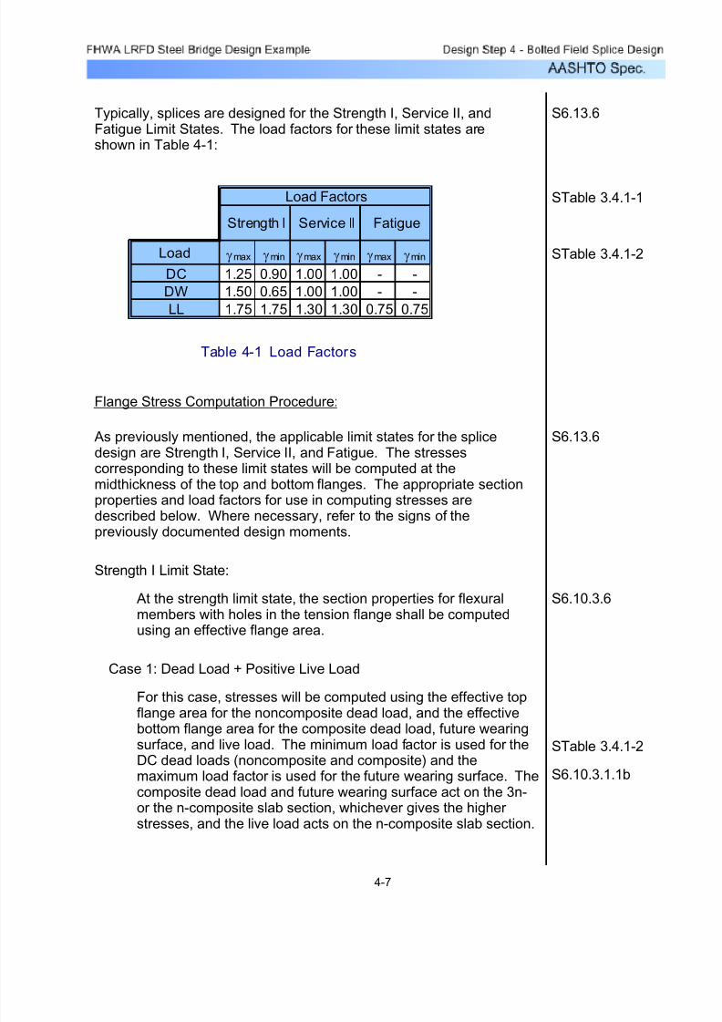
7/29/2019 LRFD steel design.pdf
http://slidepdf.com/reader/full/lrfd-steel-designpdf 206/646
S6.10.3.1.1b
STable 3.4.1-2
For this case, stresses will be computed using the effective top
flange area for the noncomposite dead load, and the effectivebottom flange area for the composite dead load, future wearingsurface, and live load. The minimum load factor is used for theDC dead loads (noncomposite and composite) and themaximum load factor is used for the future wearing surface. Thecomposite dead load and future wearing surface act on the 3n-or the n-composite slab section, whichever gives the higher stresses, and the live load acts on the n-composite slab section.
Case 1: Dead Load + Positive Live Load
S6.10.3.6 At the strength limit state, the section properties for flexuralmembers with holes in the tension flange shall be computedusing an effective flange area.
Strength I Limit State:
S6.13.6 As previously mentioned, the applicable limit states for the splicedesign are Strength I, Service II, and Fatigue. The stressescorresponding to these limit states will be computed at themidthickness of the top and bottom flanges. The appropriate sectionproperties and load factors for use in computing stresses aredescribed below. Where necessary, refer to the signs of the
previously documented design moments.
Flange Stress Computation Procedure:
Table 4-1 Load Factors
STable 3.4.1-2
STable 3.4.1-1
Load γmax γmin γmax γmin γmax γmin
DC 1.25 0.90 1.00 1.00 - -
DW 1.50 0.65 1.00 1.00 - -
LL 1.75 1.75 1.30 1.30 0.75 0.75
FatigueStrength I Service II
Load Factors
S6.13.6Typically, splices are designed for the Strength I, Service II, andFatigue Limit States. The load factors for these limit states areshown in Table 4-1:
4-7

7/29/2019 LRFD steel design.pdf
http://slidepdf.com/reader/full/lrfd-steel-designpdf 207/646
For this case, stresses will be computed using the grosssteel section. The live load acts on the n-compositeslab section.
S6.10.3.1.1cCase 2: Negative Live Load
For this case, stresses will be computed using the grosssteel section. The live load acts on the n-composite slabsection.
Case 1: Positive Live Load
C6.13.6.1.4aFatigue Limit State:
For this case, stresses will be computed using the gross steelsection. The future wearing surface is excluded. Thecomposite dead load acts on the 3n- or n-composite slabsection, whichever gives the larger stresses. The live load actson the n-composite slab section.
S6.10.3.1.1cCase 2: Dead Load + Negative Live Load
For this case, stresses will be computed using the gross steelsection. The future wearing surface is included and acts,along with the composite dead load, on the 3n- or n-composite slab section, whichever gives the higher stresses. The live load acts on the n-composite slab section.
Case 1: Dead Load + Positive Live Load
S6.13.6.1.4aService II Limit State:
For this case, stresses will be computed using the effective topflange area for all loads. The future wearing surface is
excluded and the maximum load factor is used for the DCdead loads. The live load acts on the composite steel girder plus longitudinal reinforcement section. The composite deadload is applied to this section as well, as a conservativeassumption for simplicity and convenience, since the net effectof the live load is to induce tension in the slab. The reinforcingsteel in the deck that is used corresponds to the negativemoment deck reinforcement shown in Figure 2-18.
Case 2: Dead Load + Negative Live Load
4-8
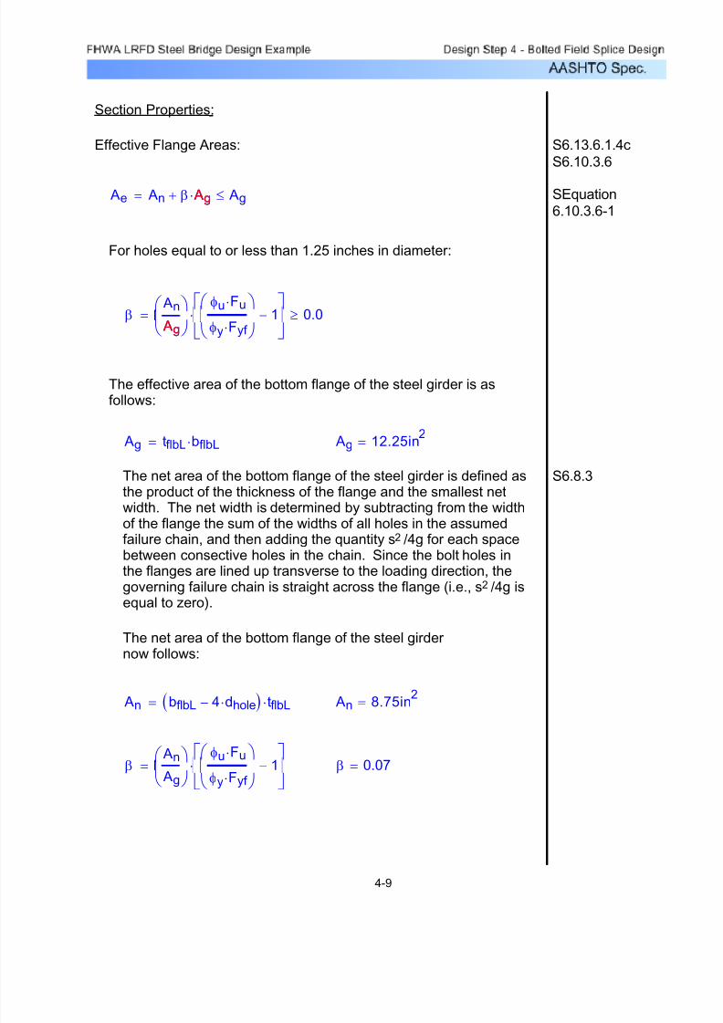
7/29/2019 LRFD steel design.pdf
http://slidepdf.com/reader/full/lrfd-steel-designpdf 208/646
β 0.07=β An
Ag
⎛
⎝
⎞
⎠
φu Fu⋅
φy Fyf ⋅
⎛
⎝
⎞
⎠1−
⎡
⎣
⎤
⎦⋅=
An 8.75in2
= An bflbL 4 dhole⋅−( ) tflbL⋅=
The net area of the bottom flange of the steel girder now follows:
S6.8.3The net area of the bottom flange of the steel girder is defined asthe product of the thickness of the flange and the smallest netwidth. The net width is determined by subtracting from the widthof the flange the sum of the widths of all holes in the assumed
failure chain, and then adding the quantity s2 /4g for each spacebetween consective holes in the chain. Since the bolt holes inthe flanges are lined up transverse to the loading direction, thegoverning failure chain is straight across the flange (i.e., s2 /4g isequal to zero).
Ag 12.25in2
= Ag tflbL bflbL⋅=
The effective area of the bottom flange of the steel girder is asfollows:
β An
Ag
⎛
⎝
⎞
⎠
φu Fu⋅
φy Fyf ⋅
⎛
⎝
⎞
⎠1−
⎡
⎣
⎤
⎦⋅ 0.0≥=
Ag
For holes equal to or less than 1.25 inches in diameter:
SEquation
6.10.3.6-1 Ae An β Ag⋅+ Ag≤= Ag
S6.13.6.1.4c
S6.10.3.6
Effective Flange Areas:
Section Properties:
4-9
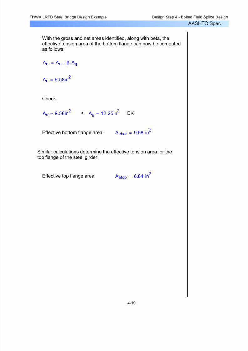
7/29/2019 LRFD steel design.pdf
http://slidepdf.com/reader/full/lrfd-steel-designpdf 209/646
With the gross and net areas identified, along with beta, theeffective tension area of the bottom flange can now be computedas follows:
Ae An β Ag⋅+=
Ae 9.58in2
=
Check:
Ae 9.58in2
= < Ag 12.25in2
= OK
Effective bottom flange area: Aebot 9.58 in2⋅=
Similar calculations determine the effective tension area for thetop flange of the steel girder:
Effective top flange area: Aetop 6.84 in2
⋅=
4-10

7/29/2019 LRFD steel design.pdf
http://slidepdf.com/reader/full/lrfd-steel-designpdf 210/646
Figure 4-2 Girder, Slab and Longitudinal Reinforcement
Neutral Axis
Y
1 2
3
4
5
The section properties for the Left Girder are calculated with the aid of Figure 4-2 shown below:
Ac3n 34.33in2= Ac3n
Weff
3ntseff ⋅=
For the 3n-composite beam:
Ac 103.00in2
= AcWeff
ntseff ⋅=
For the n-composite beam:
n 8=Modular Ratio:
Weff 103in=Effective Slab Width:
where:
Ac= Effective Slab Width x tseff
Modular Ratio
The transformed effective area of the concrete flange of the steelgirder is now determined. This requires the modular ratio as follows:
4-11

7/29/2019 LRFD steel design.pdf
http://slidepdf.com/reader/full/lrfd-steel-designpdf 211/646
The following tables contain the section properties for the left (i.e.,smaller) girder section at the splice location. The properties in Table4-2 are based on the gross area of the steel girder, and theseproperties are used for computation of stresses for the Service II and
Fatigue Limit States. The properties in Tables 4-3 and 4-4 are basedon the effective top flange and effective bottom flange of the steelgirder, respectively, and these properties are used for computation of stresses for the Strength I Limit State.
Top flange 8.750 55.188 482.9 0.3 7530.2 7530.5
Web 27.000 27.875 752.6 6561.0 110.5 6671.5Bottom flange 12.250 0.438 5.4 0.8 7912.0 7912.7
Total 48.000 25.852 1240.9 6562.1 15552.7 22114.8
Girder 48.000 25.852 1240.9 22114.8 11134.4 33249.2
Slab 34.333 62.375 2141.5 183.1 15566.5 15749.6
Total 82.333 41.082 3382.4 22297.9 26700.8 48998.7
Girder 48.000 25.852 1240.9 22114.8 29792.4 51907.2
Slab 103.000 62.375 6424.6 549.3 13883.8 14433.2
Total 151.000 50.765 7665.5 22664.1 43676.2 66340.3
Girder only 25.414 29.336 885.4 870.2 753.8 762.0
Composite (3n) 40.644 14.106 1218.7 1205.5 3473.7 3552.4
Composite (n) 50.327 4.423 1329.7 1318.2 15000.3 16140.8
Sbotmid
(Inches3)
Stopmid
(Inches3)
Stopweb
(Inches3)
Girder only:
Composite (3n):
Composite (n):
Section
ybotmid
(Inches)
ytopmid
(Inches)
Sbotweb
(Inches3)
Gross Section Properties
Section Area, A
(Inches2)
Centroid, d
(Inches)
A*d
(Inches3)
Io
(Inches4)
A*y2
(Inches4)
Itotal
(Inches4)
Table 4-2 Section Properties Based on Gross Steel Section
4-12
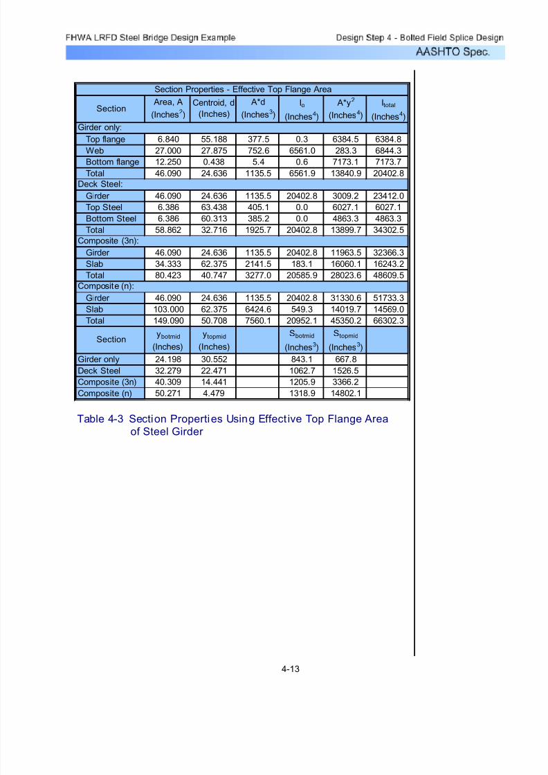
7/29/2019 LRFD steel design.pdf
http://slidepdf.com/reader/full/lrfd-steel-designpdf 212/646
Top flange 6.840 55.188 377.5 0.3 6384.5 6384.8
Web 27.000 27.875 752.6 6561.0 283.3 6844.3
Bottom flange 12.250 0.438 5.4 0.6 7173.1 7173.7
Total 46.090 24.636 1135.5 6561.9 13840.9 20402.8
Girder 46.090 24.636 1135.5 20402.8 3009.2 23412.0
Top Steel 6.386 63.438 405.1 0.0 6027.1 6027.1
Bottom Steel 6.386 60.313 385.2 0.0 4863.3 4863.3
Total 58.862 32.716 1925.7 20402.8 13899.7 34302.5
Girder 46.090 24.636 1135.5 20402.8 11963.5 32366.3
Slab 34.333 62.375 2141.5 183.1 16060.1 16243.2
Total 80.423 40.747 3277.0 20585.9 28023.6 48609.5
Girder 46.090 24.636 1135.5 20402.8 31330.6 51733.3
Slab 103.000 62.375 6424.6 549.3 14019.7 14569.0
Total 149.090 50.708 7560.1 20952.1 45350.2 66302.3
Girder only 24.198 30.552 843.1 667.8
Deck Steel 32.279 22.471 1062.7 1526.5
Composite (3n) 40.309 14.441 1205.9 3366.2
Composite (n) 50.271 4.479 1318.9 14802.1
Girder only:
Section Properties - Effective Top Flange Area
Section Area, A
(Inches2)
Centroid, d
(Inches)
A*d
(Inches3)
Io
(Inches4)
A*y2
(Inches4)
Itotal
(Inches4)
Deck Steel:
Composite (3n):
Sbotmid
(Inches3)
Stopmid
(Inches3)
Composite (n):
Sectionybotmid
(Inches)
ytopmid
(Inches)
Table 4-3 Section Properties Using Effect ive Top Flange Area
of Steel Girder
4-13
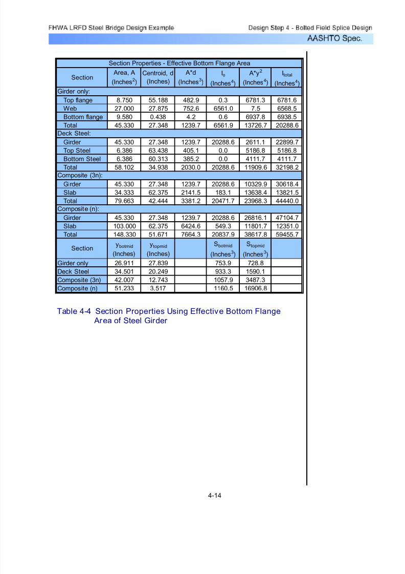
7/29/2019 LRFD steel design.pdf
http://slidepdf.com/reader/full/lrfd-steel-designpdf 213/646
Top flange 8.750 55.188 482.9 0.3 6781.3 6781.6Web 27.000 27.875 752.6 6561.0 7.5 6568.5
Bottom flange 9.580 0.438 4.2 0.6 6937.8 6938.5
Total 45.330 27.348 1239.7 6561.9 13726.7 20288.6
Girder 45.330 27.348 1239.7 20288.6 2611.1 22899.7
Top Steel 6.386 63.438 405.1 0.0 5186.8 5186.8
Bottom Steel 6.386 60.313 385.2 0.0 4111.7 4111.7
Total 58.102 34.938 2030.0 20288.6 11909.6 32198.2
Girder 45.330 27.348 1239.7 20288.6 10329.9 30618.4
Slab 34.333 62.375 2141.5 183.1 13638.4 13821.5
Total 79.663 42.444 3381.2 20471.7 23968.3 44440.0
Girder 45.330 27.348 1239.7 20288.6 26816.1 47104.7
Slab 103.000 62.375 6424.6 549.3 11801.7 12351.0
Total 148.330 51.671 7664.3 20837.9 38617.8 59455.7
Girder only 26.911 27.839 753.9 728.8
Deck Steel 34.501 20.249 933.3 1590.1
Composite (3n) 42.007 12.743 1057.9 3487.3
Composite (n) 51.233 3.517 1160.5 16906.8
Section Properties - Effective Bottom Flange Area
Section Area, A
(Inches2)
Centroid, d
(Inches)
A*d
(Inches3)
Io
(Inches4)
A*y2
(Inches4)
Itotal
(Inches4)
Girder only:
Composite (n):
Sectionybotmid
(Inches)
ytopmid
(Inches)
Deck Steel:
Composite (3n):
Sbotmid
(Inches3)
Stopmid
(Inches3)
Table 4-4 Section Properties Using Effective Bottom Flange
Area of Steel Girder
4-14
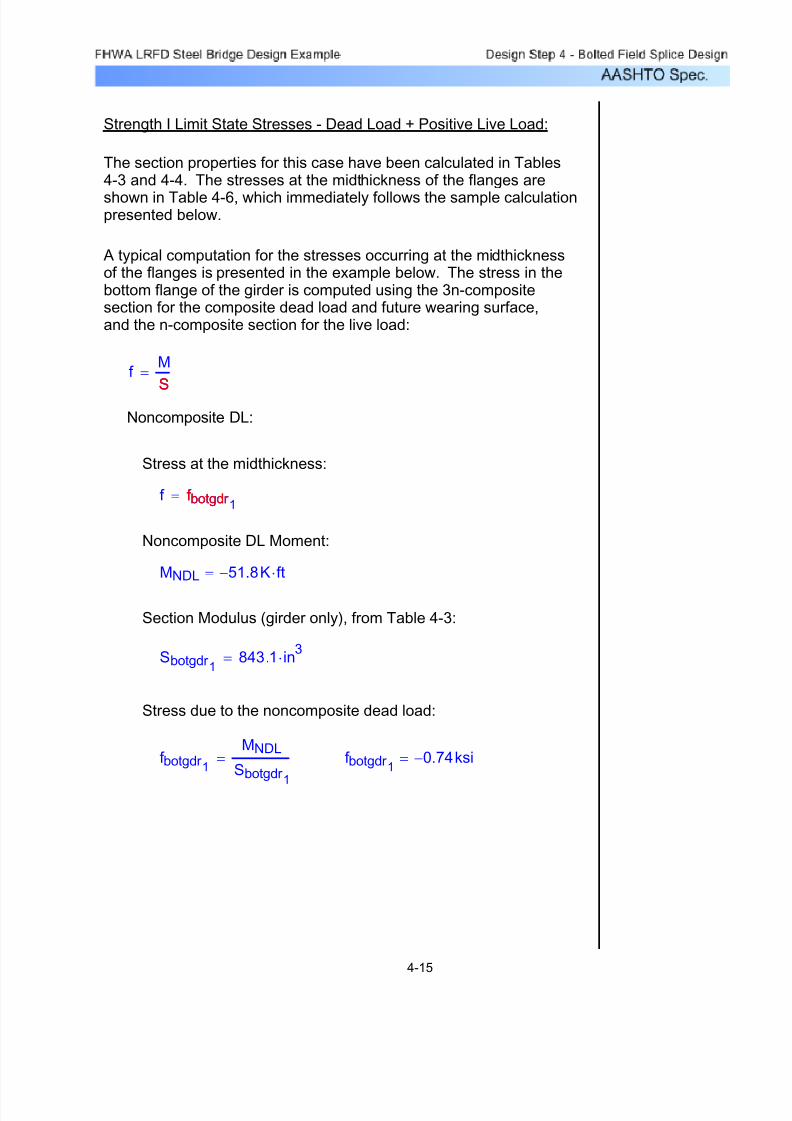
7/29/2019 LRFD steel design.pdf
http://slidepdf.com/reader/full/lrfd-steel-designpdf 214/646
Strength I Limit State Stresses - Dead Load + Positive Live Load:
The section properties for this case have been calculated in Tables4-3 and 4-4. The stresses at the midthickness of the flanges are
shown in Table 4-6, which immediately follows the sample calculationpresented below.
A typical computation for the stresses occurring at the midthicknessof the flanges is presented in the example below. The stress in thebottom flange of the girder is computed using the 3n-compositesection for the composite dead load and future wearing surface,and the n-composite section for the live load:
f M
S=
S
Noncomposite DL:
Stress at the midthickness:
f f botgdr 1= f botgdr
Noncomposite DL Moment:
MNDL 51.8− K ft⋅=
Section Modulus (girder only), from Table 4-3:
Sbotgdr 1
843.1 in3
⋅=
Stress due to the noncomposite dead load:
f botgdr 1
MNDL
Sbotgdr
1
= f botgdr 10.74− ksi=
4-15

7/29/2019 LRFD steel design.pdf
http://slidepdf.com/reader/full/lrfd-steel-designpdf 215/646
f botgdr 30.21ksi=f botgdr 3
MFWS
Sbotgdr 3
=
Stress due to the composite dead load:
Sbotgdr 31057.9 in3⋅=
Section Modulus (3n-composite), From Table 4-4:
MFWS 18.8K ft⋅=
FWS Moment:
f f botgdr 3=
3
Stress at the midthickness:
Future Wearing Surface:
f botgdr 20.18ksi=f botgdr 2
MCDL
Sbotgdr 2
=
Stress due to the composite dead load:
Sbotgdr 21057.9 in
3⋅=
Section Modulus (3n-composite), From Table 4-4:
MCDL 15.5K ft⋅=
Composite DL Moment:
f f botgdr 2= 2
Stress at the midthickness:
Composite DL:
4-16

7/29/2019 LRFD steel design.pdf
http://slidepdf.com/reader/full/lrfd-steel-designpdf 216/646
Positive Live Load:
Stress at the midthickness:
f f botgdr 4= 4
Live Load Moment:
MPLL 1307.8K ft⋅=
Section Modulus (n-composite), From Table 4-4:
Sbotgdr 41160.5 in
3⋅=
Stress due to the positive live load:
f botgdr 4
MPLL
Sbotgdr 4
= f botgdr 413.52ksi=
The preceding stresses are now factored by their respective loadfactors to obtain the final factored stress at the midthickness of thebottom flange for this load case. The applicable load factors for this
case were discussed previously.
STable 3.4.1-1
STable 3.4.1-2
f botgdr 0.90 f botgdr 1⋅ 0.90 f botgdr 2
⋅+ 1.50 f botgdr 3⋅+ 1.75 f botgdr 4
⋅+( )=
f botgdr 23.48ksi=
The stresses at the midthickness of the top flange for this load caseare computed in a similar manner. The section properties used to
obtain the stresses in the top flange are also from Tables 4-3 and 4-4.
4-17

7/29/2019 LRFD steel design.pdf
http://slidepdf.com/reader/full/lrfd-steel-designpdf 217/646
The top and bottom flange midthickness stresses are summarized inTable 4-5, shown below.
LoadingMoment
(K-ft)
f botmid
(ksi)
f topmid
(ksi)
Noncomposite DL -51.80 -0.74 0.93
Composite DL 15.50 0.18 -0.05
FWS DL 18.80 0.21 -0.06
Live Load - HL-93 1307.80 13.52 -0.93
Strength I 2284.18 23.48 -0.93
Strength I - Dead Load + Positive Live LoadSummary of Unfactored Values
Summary of Factored Values
Limit State
Table 4-5 Strength I Flange Stresses for Dead + Pos. LL
The computation of the midthickness flange stresses for the remainingload cases are computed in a manner similar to what was shown in thesample calculation that preceded Table 4-5.
Strength I Limit State - Dead Load + Negative Live Load:
The computed stresses in the following table require the use of sectionproperties from Table 4-3.
LoadingMoment
(K-ft)
f botmid
(ksi)
f topmid
(ksi)
Noncomposite DL -51.80 -0.74 0.93Composite DL 15.50 0.18 -0.12
Live Load - HL-93 -953.30 -10.76 7.49
Strength I -1713.65 -19.54 14.13
Strength I - Dead Load + Negative Live Load
Summary of Unfactored Values
Summary of Factored Values
Limit State
Table 4-6 Strength I Flange Stresses for Dead + Neg. LL
4-18

7/29/2019 LRFD steel design.pdf
http://slidepdf.com/reader/full/lrfd-steel-designpdf 218/646
Service II Limit State - Dead Load + Positive Live Load:
The computed stresses in the following table require the use of sectionproperties from Table 4-2.
LoadingMoment
(K-ft)
f botmid
(ksi)
f topmid
(ksi)
Noncomposite DL -51.80 -0.71 0.82
Composite DL 15.50 0.15 -0.05
FWS 18.80 0.19 -0.06
Live Load - HL-93 1307.80 11.91 -1.05
Service II 1682.64 15.10 -0.65
Service II - Dead Load + Positive Live Load
Summary of Unfactored Values
Summary of Factored Values
Limit State
Table 4-7 Service II Flange Stresses for Dead + Pos. LL
Service II Limit State - Dead Load + Negative Live Load:
The computed stresses in the following table require the use of sectionproperties from Table 4-2.
LoadingMoment
(K-ft)
f botmid
(ksi)
f topmid
(ksi)
Noncomposite DL -51.80 -0.71 0.82
Composite DL 15.50 0.14 -0.01
Live Load - HL-93 -953.30 -8.68 0.76
Service II -1275.59 -11.85 1.80
Summary of Factored Values
Limit State
Service II - Dead Load + Negative Live Load
Summary of Unfactored Values
Table 4-8 Service II Flange Stresses for Dead + Neg. LL
4-19

7/29/2019 LRFD steel design.pdf
http://slidepdf.com/reader/full/lrfd-steel-designpdf 219/646
Fatigue Limit State - Positive Live Load:
The computed stresses in the following table require the use of sectionproperties from Table 4-2.
LoadingMoment
(K-ft)
f botmid
(ksi)
f topmid
(ksi)
Live Load-Fatigue 394.30 3.59 -0.32
Fatigue 295.73 2.69 -0.24
Fatigue - Positive Live Load
Summary of Unfactored Values
Summary of Factored Values
Limit State
Table 4-9 Fatigue Flange Stresses for Posi tive LL
Fatigue Limit State - Negative Live Load:
The computed stresses in the following table require the use of sectionproperties from Table 4-2.
LoadingMoment
(K-ft)
f botmid
(ksi)
f topmid
(ksi)
Live Load-Fatigue -284.00 -2.59 0.23
Fatigue -213.00 -1.94 0.17
Fatigue - Negative Live Load
Summary of Unfactored Values
Summary of Factored Values
Limit State
Table 4-10 Fatigue Flange Stresses for Negative LL
4-20
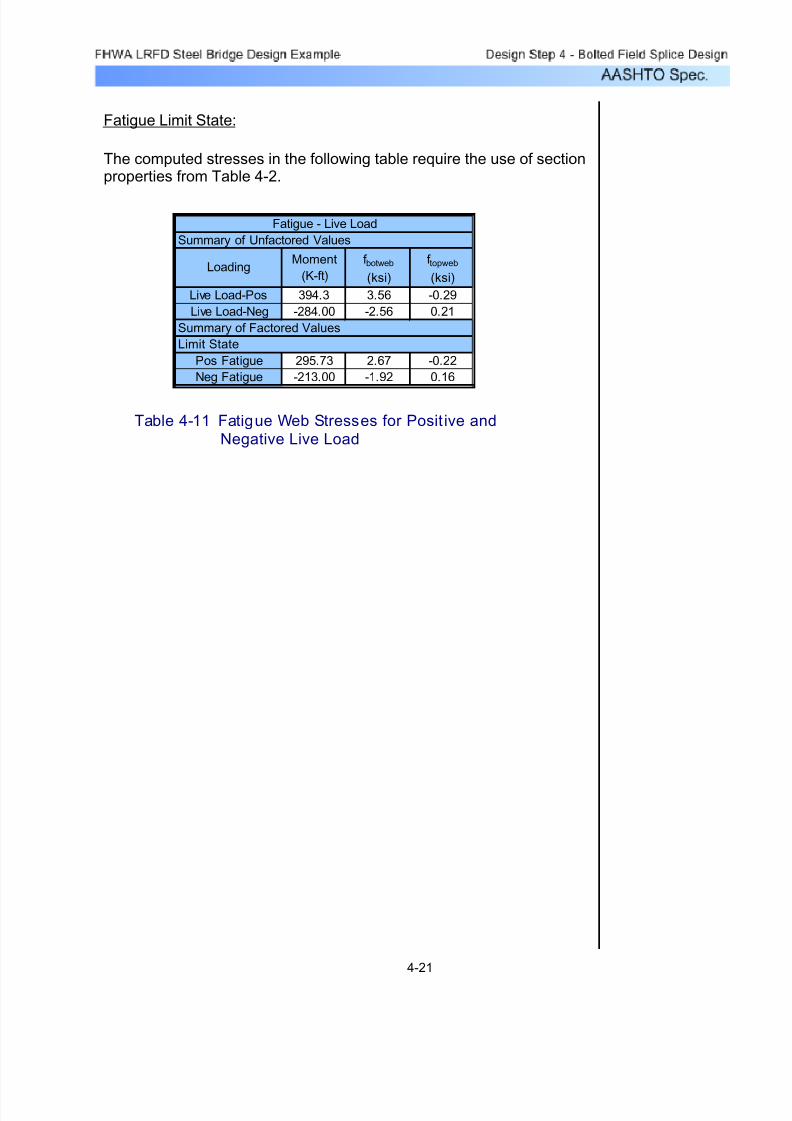
7/29/2019 LRFD steel design.pdf
http://slidepdf.com/reader/full/lrfd-steel-designpdf 220/646
Fatigue Limit State:
The computed stresses in the following table require the use of sectionproperties from Table 4-2.
LoadingMoment
(K-ft)
f botweb
(ksi)
f topweb
(ksi)
Live Load-Pos 394.3 3.56 -0.29
Live Load-Neg -284.00 -2.56 0.21
Pos Fatigue 295.73 2.67 -0.22
Neg Fatigue -213.00 -1.92 0.16
Fatigue - Live Load
Summary of Unfactored Values
Summary of Factored Values
Limit State
Table 4-11 Fatigue Web Stresses for Posit ive and
Negative Live Load
4-21

7/29/2019 LRFD steel design.pdf
http://slidepdf.com/reader/full/lrfd-steel-designpdf 221/646
A summary of the factored stresses at the midthickness of the topand bottom flanges for the Strength I, Service II, and Fatigue limitstates are presented below in Tables 4-12 through 4-14. Table4-14 also contains the top and bottom web fatigue stresses.
Limit State Location Dead + Pos. LL Dead + Neg. LL
Bottom Flange 23.48 -19.54
Top Flange -0.93 14.13Strength I
Stress (ksi)
Table 4-12 Strength I Flange Stresses
Limit State Location Dead + Pos. LL Dead + Neg. LL
Bottom Flange 15.10 -11.85
Top Flange -0.65 1.80Service II
Stress (ksi)
Table 4-13 Service II Flange Stresses
Limit State Location Positive LL Negative LL
Bottom Flange 2.69 -1.94
Top Flange -0.24 0.17
Bottom of Web 2.67 -1.92
Top of Web -0.22 0.16
Stress (ksi)
Fatigue
Table 4-14 Fatigue Flange and Web Stresses
4-22

7/29/2019 LRFD steel design.pdf
http://slidepdf.com/reader/full/lrfd-steel-designpdf 222/646
Fyf 50ksi=Minimum yield strength of the flange:
φf 1.0=Resistance factor for flexure(Design Step 4.1):
α 1.0=Flange stress reduction
factor:
Rh 1.0=Hybrid girder reduction factor.For homogeneous girders:
f cf 23.48 ksi⋅=Maximum flexural stress due to thefactored loads at the midthickness of the controlling flange at the point of splice (from Table 4-12):
where:
SEquation
6.13.6.1.4c-1Fcf
f cf
Rhα φf ⋅ Fyf ⋅+
⎛
⎝
⎞
⎠2
0.75 α⋅ φf ⋅ Fyf ⋅≥=
α
The minimum design stress for the controlling (bottom) flange iscomputed as follows:
The calculation of the minimum design force is presented below for
the load case of dead load with positive live load.
S6.10.3.6
The minimum design force for the controlling flange, Pcu, is takenequal to the design stress, Fcf , times the smaller effective flangearea, Ae, on either side of the splice. When a flange is incompression, the effective compression flange area shall betaken as Ae = Ag.
The next step is to determine the minimum design forces for thecontrolling flange of each load case (i.e., positive and negative live
load). By inspection of Table 4-12, it is obvious that the bottomflange is the controlling flange for both positive and negative liveload for the Strength I Limit State.
S6.13.6.1.4cStrength I Minimum Design Force - Controlling Flange:
4-23
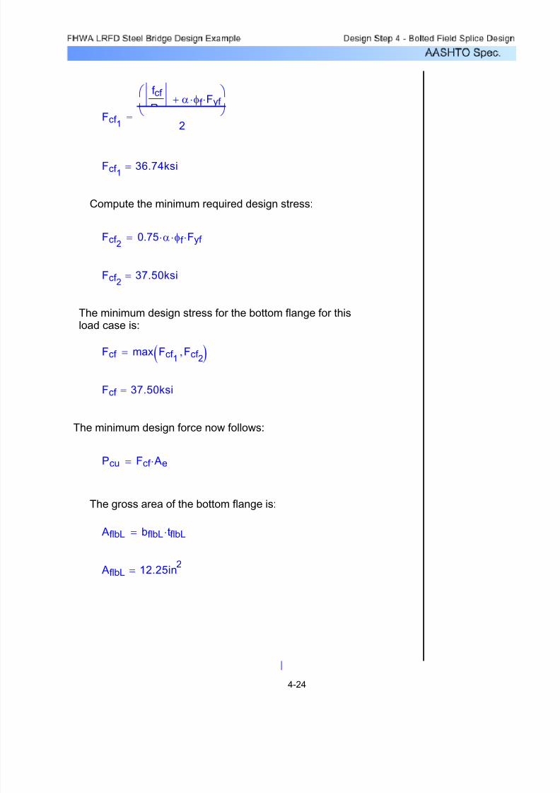
7/29/2019 LRFD steel design.pdf
http://slidepdf.com/reader/full/lrfd-steel-designpdf 223/646
Fcf 1
f cf
Rhα φf ⋅ Fyf ⋅+
⎛
⎝
⎞
⎠2
=
Fcf 136.74ksi=
Compute the minimum required design stress:
Fcf 2
0.75 α⋅ φf ⋅ Fyf ⋅=
Fcf 2 37.50ksi=
The minimum design stress for the bottom flange for thisload case is:
Fcf max Fcf 1Fcf 2
,( )=
Fcf 37.50ksi=
The minimum design force now follows:
Pcu Fcf Ae⋅=
The gross area of the bottom flange is:
AflbL bflbL tflbL⋅=
AflbL 12.25in2
=
4-24

7/29/2019 LRFD steel design.pdf
http://slidepdf.com/reader/full/lrfd-steel-designpdf 224/646
Since the bottom flange force for this load case is a tensile force,the effective area will be used. This value was computed previouslyto be:
Aebot 9.58in2=
Therefore:
Pcu Fcf Aebot⋅=
Pcu 359.25K=
Table 4-15 presents the minimum design forces for the Strength I LimitState for both the positive and negative live load cases.
Load Case Location f cf (ksi) Fcf (ksi) Area (in2) Pcu (kips)
Dead + Pos. LL Bot. Flange 23.48 37.5 9.58 359.25
Dead + Neg. LL Bot. Flange -19.54 37.5 12.25 459.38
Strength I Limit State
Controlling Flange
Table 4-15 Contro ll ing Flange Forces
In the above table, the design controlling flange force (Pcu) is acompressive force for negative live load.
4-25

7/29/2019 LRFD steel design.pdf
http://slidepdf.com/reader/full/lrfd-steel-designpdf 225/646
Rh 1.00=Hybrid girder reduction factor:
Rcf 1.60=Rcf Fcf
f cf =
Controlling flange stress ratio:
f cf 23.48ksi=Controlling flange actual stress:
Fcf 37.50ksi=Controlling flange design stress:
f ncf 0.93− ksi⋅=Maximum flexural stress due to thefactored loads at the midthickness of the noncontrolling flange at the pointof splice concurrent with f cf (see Table4-12):
where:
SEquation
6.13.6.1.4c-2Fncf Rcf
f ncf
Rh⋅ 0.75 α⋅ φf ⋅ Fyf ⋅≥=
f ncf
The minimum design stress for the noncontrolling (top) flange iscomputed as follows:
The calculation of the minimum design force is presented below for the load case of dead load with positive live load.
S6.10.3.6
The minimum design force for the noncontrolling flange, Pncu, istaken equal to the design stress, Fncf , times the smaller effectiveflange area, Ae, on either side of the splice. When a flange is incompression, the effective compression flange area shall betaken as Ae = Ag.
The next step is to determine the minimum design forces for thenoncontrolling flange of each load case (i.e., positive and negative
live load). By inspection of Table 4-12, the top flange is thenoncontrolling flange for both positive and negative live load for theStrength I Limit State.
S6.13.6.1.4cStrength I Minimum Design Force - Noncontrolling Flange:
4-26

7/29/2019 LRFD steel design.pdf
http://slidepdf.com/reader/full/lrfd-steel-designpdf 226/646
(compression)Pncu 328.13K=
Pncu Fncf Ag⋅=
Therefore:
Ag 8.75in2
= Ag tfltL bfltL⋅=
SEquation
6.10.3.6-2 Ae Ag=
For the positive live load case, the top flange is in compression.The effective compression flange area shall be taken as:
Pncu Fncf Ae⋅=
The minimum design force now follows:
Fncf 37.50ksi=
Fncf max Fncf 1Fncf 2
,( )=
The minimum design stress in the top flange is:
Fncf 2
37.50ksi=
Fncf 20.75 α⋅ φf ⋅ Fyf ⋅=
Compute the minimum required design stress:
Fncf 11.49ksi=
Fncf 1Rcf
f ncf
Rh⋅=
Therefore:
4-27
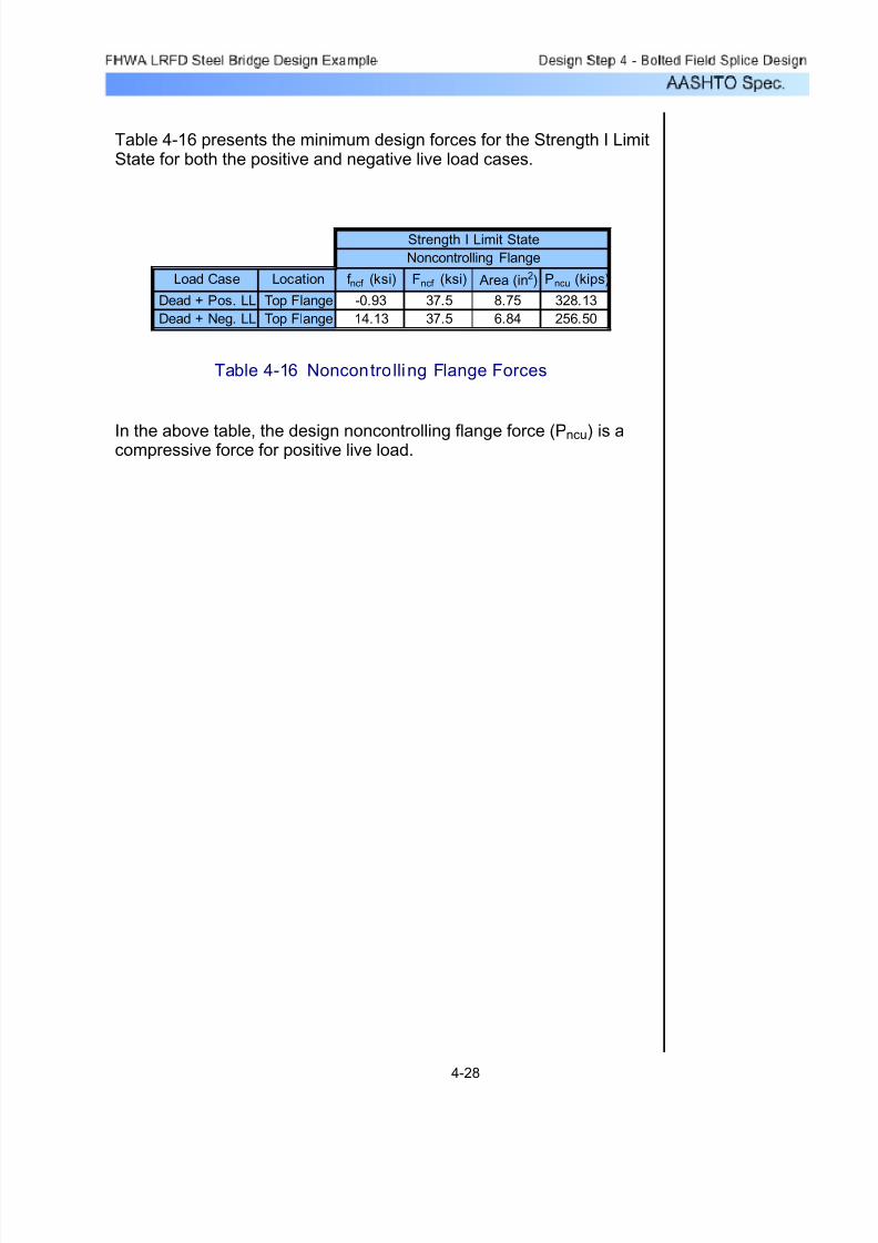
7/29/2019 LRFD steel design.pdf
http://slidepdf.com/reader/full/lrfd-steel-designpdf 227/646
Table 4-16 presents the minimum design forces for the Strength I LimitState for both the positive and negative live load cases.
Load Case Location f ncf (ksi) Fncf (ksi) Area (in2) Pncu (kips)
Dead + Pos. LL Top Flange -0.93 37.5 8.75 328.13
Dead + Neg. LL Top Flange 14.13 37.5 6.84 256.50
Strength I Limit State
Noncontrolling Flange
Table 4-16 Noncontro lling Flange Forces
In the above table, the design noncontrolling flange force (Pncu) is acompressive force for positive live load.
4-28

7/29/2019 LRFD steel design.pdf
http://slidepdf.com/reader/full/lrfd-steel-designpdf 228/646
Service II Limit State Flange Forces: S6.13.6.1.4c
Per the Specifications, bolted connections for flange splices are to
be designed as slip-critical connections for the service level flangedesign force. This design force shall be taken as the Service IIdesign stress, Fs, multiplied by the smaller gross flange area oneither side of the splice.
Fs is defined as follows:
Fsf s
Rh=
f sSEquation
6.13.6.1.4c-4
f s = maximum flexural Service II stress at the midthickness of theflange under consideration.
The factored Service II design stresses and forces are shown in Table4-17 below.
Load Case Location Fs (ksi) Agross (in
2
) Ps (kips)Bot. Flange 15.10 12.25 184.98
Top Flange -0.65 8.75 -5.69
Bot. Flange -11.85 12.25 -145.16
Top Flange 1.80 8.75 15.75
Service II Limit State
Dead + Pos. LL
Dead + Neg. LL
Table 4-17 Service II Flange Forces
It is important to note here that the flange slip resistance must exceed
the larger of: (1) the Service II flange forces or (2) the factored flangeforces from the moments at the splice due to constructibility (erectionand/or deck pouring sequence). However, in this design example,no special erection procedure is prescribed and, per the Introductionin Design Step 1, the deck is placed in a single pour. Therefore, theconstructibility moment is equal to the noncomposite dead loadmoment shown at the beginning of this design step. By inspection,the Service II Limit State will control for checking of slip-criticalconnections for the flanges and the web in this example.
S3.4.2
4-29
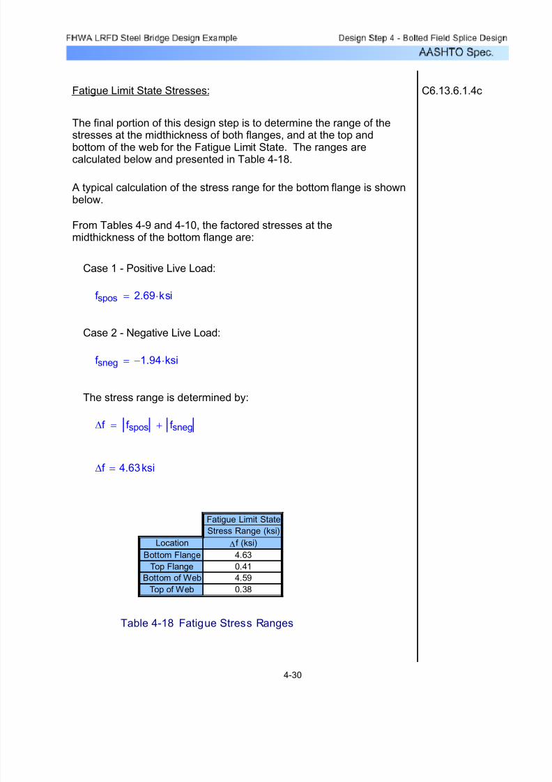
7/29/2019 LRFD steel design.pdf
http://slidepdf.com/reader/full/lrfd-steel-designpdf 229/646
Fatigue Limit State Stresses: C6.13.6.1.4c
The final portion of this design step is to determine the range of the
stresses at the midthickness of both flanges, and at the top andbottom of the web for the Fatigue Limit State. The ranges arecalculated below and presented in Table 4-18.
A typical calculation of the stress range for the bottom flange is shownbelow.
From Tables 4-9 and 4-10, the factored stresses at themidthickness of the bottom flange are:
Case 1 - Positive Live Load:
f spos 2.69 ksi⋅=
Case 2 - Negative Live Load:
f sneg 1.94− ksi⋅=
The stress range is determined by:
∆f f spos f sneg+=
∆f 4.63ksi=
Fatigue Limit State
Stress Range (ksi)
Location
∆f (ksi)
Bottom Flange 4.63
Top Flange 0.41
Bottom of Web 4.59
Top of Web 0.38
Table 4-18 Fatigue Stress Ranges
4-30
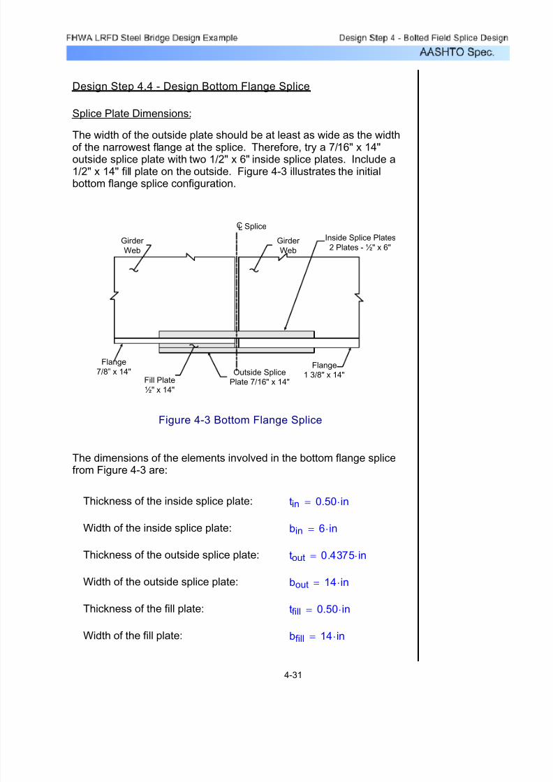
7/29/2019 LRFD steel design.pdf
http://slidepdf.com/reader/full/lrfd-steel-designpdf 230/646
bfill 14 in⋅=Width of the fill plate:
tfill 0.50 in⋅=Thickness of the fill plate:
bout 14 in⋅=Width of the outside splice plate:
tout 0.4375 in⋅=Thickness of the outside splice plate:
bin 6 in⋅=Width of the inside splice plate:
tin 0.50 in⋅=Thickness of the inside splice plate:
The dimensions of the elements involved in the bottom flange splicefrom Figure 4-3 are:
Figure 4-3 Bottom Flange Splice
Girder
Web
Girder
Web
CL Splice
Inside Splice Plates
2 Plates - ½" x 6"
Flange
7/8” x 14"Flange
1 3/8" x 14"Outside Splice
Plate 7/16" x 14"Fill Plate
½" x 14"
The width of the outside plate should be at least as wide as the widthof the narrowest flange at the splice. Therefore, try a 7/16" x 14"outside splice plate with two 1/2" x 6" inside splice plates. Include a1/2" x 14" fill plate on the outside. Figure 4-3 illustrates the initialbottom flange splice configuration.
Splice Plate Dimensions:
Design Step 4.4 - Design Bottom Flange Splice
4-31

7/29/2019 LRFD steel design.pdf
http://slidepdf.com/reader/full/lrfd-steel-designpdf 231/646
If the combined area of the inside splice plates is within tenpercent of the area of the outside splice plate, then both the insideand outside splice plates may be designed for one-half the flangedesign force.
C6.13.6.1.4c
Gross area of the inside and outside splice plates:
Inside:
Agross_in 2 tin⋅ bin⋅=
Agross_in 6.00in2=
Outside:
Agross_out tout bout⋅=
Agross_out 6.13in2
=
Check:
1
Agross_in
Agross_out−
⎛
⎝
⎞
⎠100⋅ % 2.04%=
The combined areas are within ten percent.
If the areas of the inside and outside splice plates had differed bymore than ten percent, the flange design force would beproportioned to the inside and outside splice plates. This iscalculated by multiplying the flange design force by the ratio of thearea of the splice plate under consideration to the total area of the
inner and outer splice plates.
C6.13.6.1.4c
4-32
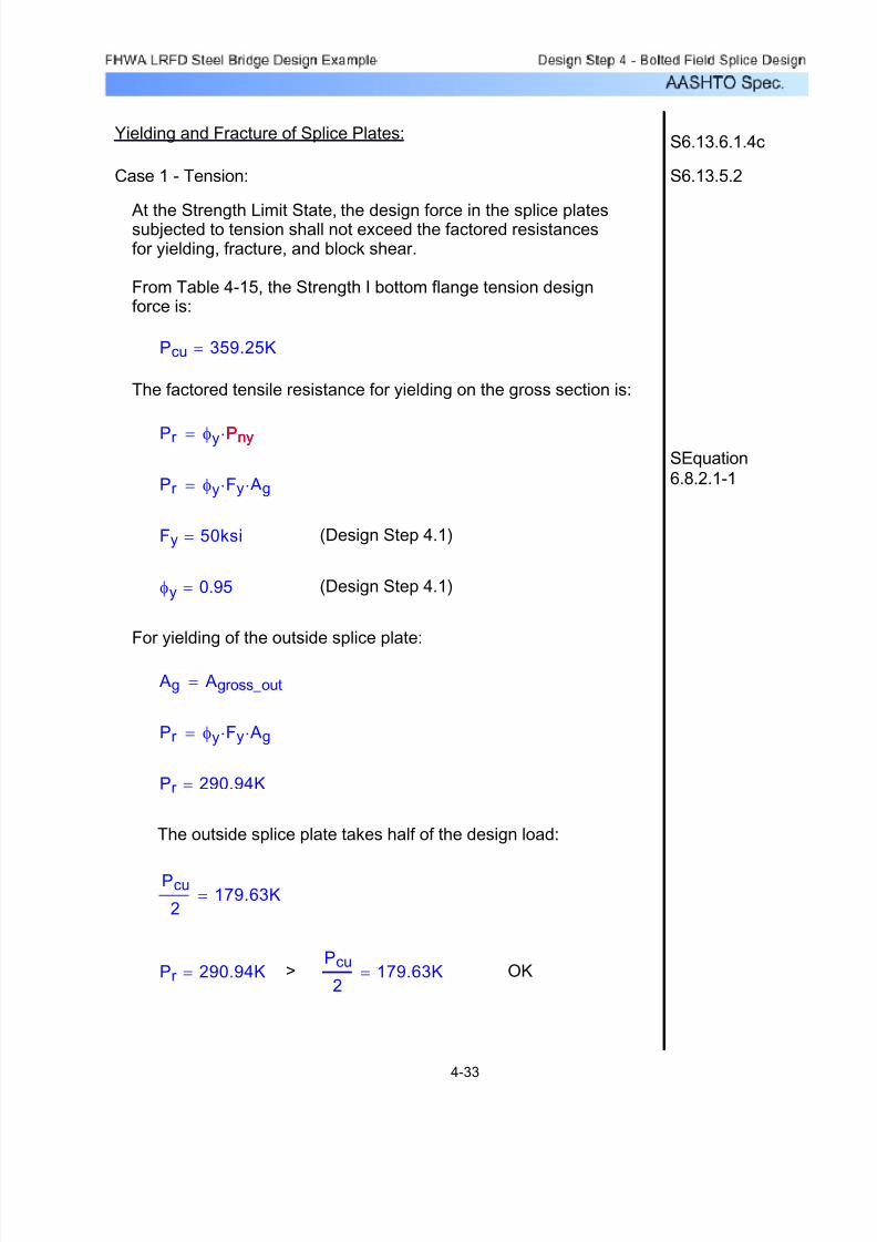
7/29/2019 LRFD steel design.pdf
http://slidepdf.com/reader/full/lrfd-steel-designpdf 232/646
OKPcu
2179.63K=>Pr 290.94K=
Pcu
2179.63K=
The outside splice plate takes half of the design load:
Pr 290.94K=
Pr φy Fy⋅ Ag⋅=
Ag Agross_out=
For yielding of the outside splice plate:
(Design Step 4.1)φy 0.95=
(Design Step 4.1)Fy 50ksi=
Pr φy Fy⋅ Ag⋅=
SEquation
6.8.2.1-1
Pr φy Pny⋅= Pny
The factored tensile resistance for yielding on the gross section is:
Pcu 359.25K=
From Table 4-15, the Strength I bottom flange tension designforce is:
At the Strength Limit State, the design force in the splice platessubjected to tension shall not exceed the factored resistancesfor yielding, fracture, and block shear.
S6.13.5.2Case 1 - Tension:
S6.13.6.1.4cYielding and Fracture of Splice Plates:
4-33

7/29/2019 LRFD steel design.pdf
http://slidepdf.com/reader/full/lrfd-steel-designpdf 233/646
S6.8.3The net width shall be determined for each chain of holesextending across the member along any transverse, diagonal
or zigzag line. This is determined by subtracting from thewidth of the element the sum of the width of all holes in thechain and adding the quantity s2/4g for each space betweenconsecutive holes in the chain. For non-staggered holes,such as in this design example, the minimum net width is thewidth of the element minus the number of bolt holes in a linestraight across the width.
To compute the net area of the splice plates, assume four 7/8" bolts across the width of the splice plate.
S6.13.5.2U 1.0=
(Design Step 4.1)φu 0.80=
(Design Step 4.1)Fu 65ksi=
Pr φu Fu⋅ An⋅ U⋅= U
SEquation
6.8.2.1-2
Pr φu Pnu⋅= Pnu
The factored tensile resistance for fracture on the net section is:
OK
Pcu
2 179.63K=>Pr 285.00K=
Pcu
2179.63K=
The inside splice plate takes half of the design load:
Pr 285.00K=
Pr φy Fy⋅ Ag⋅=
Ag Agross_in=
For yielding of the inside splice plates:
4-34

7/29/2019 LRFD steel design.pdf
http://slidepdf.com/reader/full/lrfd-steel-designpdf 234/646
OKP
cu2
179.63K=>Pr 227.50K=
The outside splice plate takes half of the design flange force:
Pr 227.50K=
Pr φu Fu⋅ An_out⋅ U⋅=
OK0.85 Agross_out
⋅ 5.21in2
=< An_out
4.38in2
=
Agross_out 6.13in2=
An 0.85 Ag⋅≤
S6.13.5.2The net area of the connecting element is limited to 0.85 Ag:
An_out 4.38in2
=
An_out bn_out tout⋅=
The nominal area is determined to be:
bn_out 10.00in=
(Design Step 4.1)dhole 1.0in=
bn_out bout 4 dhole⋅−=
The net width is:
For fracture of the outside splice plate:
4-35

7/29/2019 LRFD steel design.pdf
http://slidepdf.com/reader/full/lrfd-steel-designpdf 235/646
OKPcu
2179.63K=>P
r 208.00K=
The inside splice plates take half of the design flange force:
Pr 208.00K=
Pr φu Fu⋅ An_in⋅ U⋅=
OK0.85 Agross_in⋅ 5.10in
2
=< An_in 4.00in
2
=
Agross_in 6.00in2=
An 0.85 Ag⋅≤
S6.13.5.2The net area of the connecting element is limited to 0.85 Ag:
An_in 4.00in
2
=
An_in 2 bn_in tin⋅( )=
The nominal area is determined to be:
bn_in 4.00in=
bn_in bin 2 dhole⋅−=
The net width is:
For fracture of the inside splice plates:
4-36

7/29/2019 LRFD steel design.pdf
http://slidepdf.com/reader/full/lrfd-steel-designpdf 236/646
OKPcu
2229.69K=>Rr_in 270.00K=
Rr_in 270.00K=
Rr_in φc Fy⋅ As⋅=
As Agross_in=
For yielding of the inside splice plates:
OKPcu
2229.69K=>Rr_out 275.63K=
Rr_out 275.63K=
Rr_out φc Fy⋅ As⋅=
As Agross_out=
For yielding of the outside splice plate:
(Design Step 4.1)φc 0.90=
SEquation
6.13.6.1.4c-3Rr φc Fy⋅ As⋅= As
The factored resistance of the splice plate is:
This force is distributed equally to the inside and outsidesplice plates.
Pcu 459.38 K⋅=
From Table 4-15, the Strength I bottom flange compressiondesign force is:
S6.13.6.1.4cCase 2 - Compression:
4-37

7/29/2019 LRFD steel design.pdf
http://slidepdf.com/reader/full/lrfd-steel-designpdf 237/646
φbs 0.80=Resistance factor for block shear:
Fu 65ksi=Minimum tensile strength of theconnected material:
Fy 50ksi=Minimum yield strength of theconnected material:
where, from Design Step 4.1:
SEquation 6.13.4-2Rr φbs 0.58 Fu⋅ Avn⋅ Fy Atg⋅+( )⋅= Atg
Otherwise:
SEquation 6.13.4-1Rr φbs 0.58 Fy⋅ Avg⋅ Fu Atn⋅+( )⋅= Atn
then: Atn 0.58 Avn⋅≥If
To determine the appropriate block shear equation:
Pcu 359.25 K⋅=
From Table 4-15, the Strength I bottom flange tension design force is:
All tension connections, including connection plates, splice platesand gusset plates, shall be investigated to ensure that adequate
connection material is provided to develop the factoredresistance of the connection. Block shear rupture will usually notgovern the design of splice plates of typical proportion. However,the block shear checks are carried out here for completeness.
S6.13.6.1.4c
S6.13.5.2S6.13.4
Block Shear:
4-38
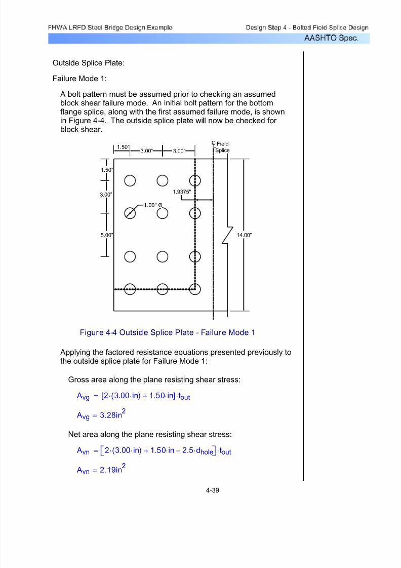
7/29/2019 LRFD steel design.pdf
http://slidepdf.com/reader/full/lrfd-steel-designpdf 238/646
Outside Splice Plate:
Failure Mode 1:
A bolt pattern must be assumed prior to checking an assumedblock shear failure mode. An initial bolt pattern for the bottomflange splice, along with the first assumed failure mode, is shownin Figure 4-4. The outside splice plate will now be checked for block shear.
14.00”
3.00”
1.50”
5.00”
1.50”3.00” 3.00”
1.9375"
1.00" Ø
FieldSplice
CL
Figure 4-4 Outside Splice Plate - Failure Mode 1
Applying the factored resistance equations presented previously tothe outside splice plate for Failure Mode 1:
Gross area along the plane resisting shear stress:
Avg 2 3.00 in⋅( )⋅ 1.50 in⋅+[ ] tout⋅=
Avg 3.28in2=
Net area along the plane resisting shear stress:
Avn 2 3.00 in⋅( )⋅ 1.50 in⋅+ 2.5 dhole⋅− tout⋅=
Avn 2.19in2=
4-39

7/29/2019 LRFD steel design.pdf
http://slidepdf.com/reader/full/lrfd-steel-designpdf 239/646
OKPcu
2179.63K=>Rr 280.88K=
Check:
Rr 280.88K=
Rr φbs 0.58 Fy⋅ Avg⋅ Fu Atn⋅+( )⋅=
Therefore, use SEquation 6.13.4-1:
0.58 Avn⋅ 1.27in2
=> Atn 3.94in2
=
To determine which equation should be applied to calculatethe factored resistance:
Atn 3.94in2
=
Atn 2 3.00 in⋅( )⋅ 5.00 in⋅+ 1.50 in⋅+[ ] 3.5 dhole⋅− tout⋅=
Net area along the plane resisting tension stress:
Atg 5.47in2
=
Atg 2 3.00 in⋅( )⋅ 5.00 in⋅+ 1.50 in⋅+[ ] tout⋅=
Gross area along the plane resisting tension stress:
4-40

7/29/2019 LRFD steel design.pdf
http://slidepdf.com/reader/full/lrfd-steel-designpdf 240/646
Failure Mode 2:
See Figure 4-5 for Failure Mode 2:
14.00”
3.00”
1.50”
5.00”
1.50”3.00” 3.00”
1.9375"
1.00” Ø
Field
Splice
CL
Figure 4-5 Outside Splice Plate - Failure Mode 2
Applying the factored resistance equations presented previously tothe outside splice plate for Failure Mode 2:
Gross area along the plane resisting shear stress:
Avg 2 2 3.00 in⋅( )⋅ 1.50 in⋅+[ ] tout⋅=
Avg 6.56in2
=
Net area along the plane resisting shear stress:
Avn 2 2 3.00 in⋅( )⋅ 1.50 in⋅+ 2.5 dhole⋅− tout⋅=
Avn 4.38in2
=
4-41

7/29/2019 LRFD steel design.pdf
http://slidepdf.com/reader/full/lrfd-steel-designpdf 241/646
OKPcu
2179.63K=>Rr 288.75K=
Check:
Rr 288.75K=
Rr φbs 0.58 Fy⋅ Avg⋅ Fu Atn⋅+( )⋅=
Therefore, use SEquation 6.13.4-1:
0.58 Avn⋅ 2.54in2
=> Atn 2.63in2
=
To determine which equation should be applied to calculatethe factored resistance:
Atn 2.63in2
=
Atn 2 3.00 in⋅ 1.50 in⋅+( ) 1.5dhole− tout⋅=
Net area along the plane resisting tension stress:
Atg 3.94in2=
Atg 2 3.00 in⋅ 1.50 in⋅+( ) tout⋅=
Gross area along the plane resisting tension stress:
4-42
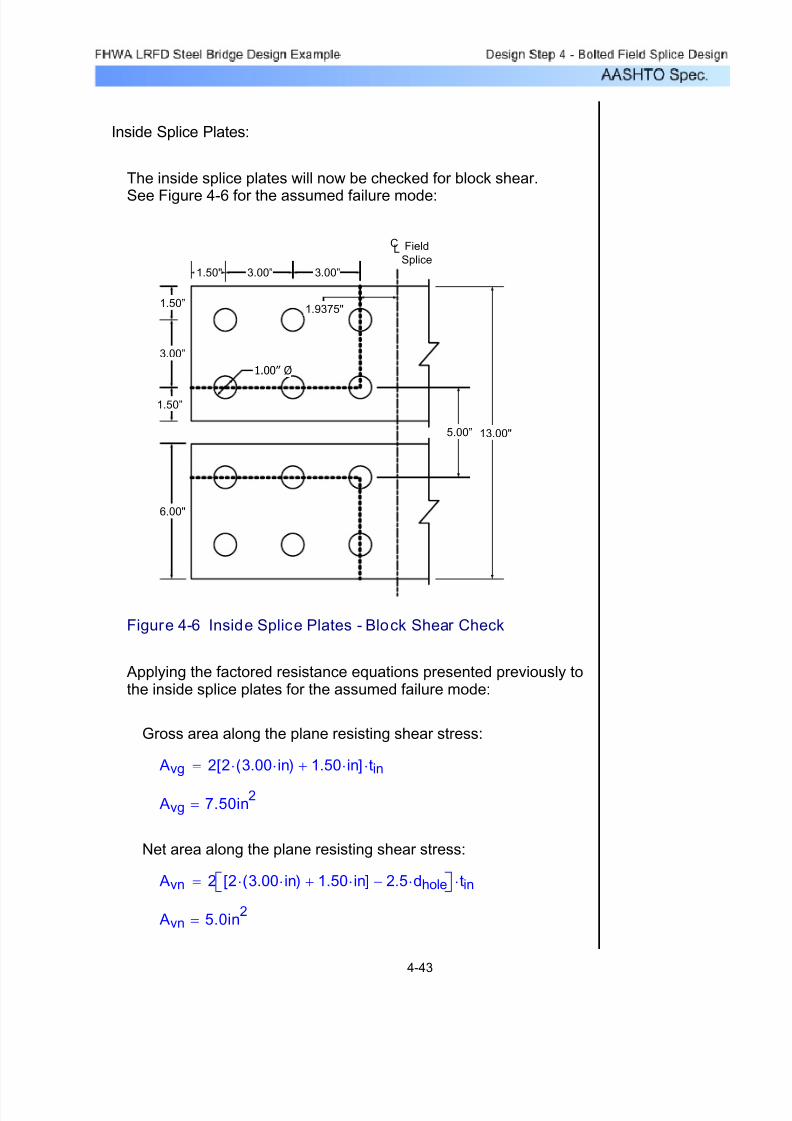
7/29/2019 LRFD steel design.pdf
http://slidepdf.com/reader/full/lrfd-steel-designpdf 242/646
Inside Splice Plates:
The inside splice plates will now be checked for block shear.
See Figure 4-6 for the assumed failure mode:
6.00"
13.00"
1.50”
3.00”
1.50”
5.00”
1.50" 3.00” 3.00”
1.9375"
1.00” Ø
CL Field
Splice
Figure 4-6 Inside Splice Plates - Block Shear Check
Applying the factored resistance equations presented previously tothe inside splice plates for the assumed failure mode:
Gross area along the plane resisting shear stress:
Avg 2 2 3.00 in⋅( )⋅ 1.50 in⋅+[ ] tin⋅=
Avg 7.50in2
=
Net area along the plane resisting shear stress:
Avn 2 2 3.00 in⋅( )⋅ 1.50 in⋅+[ ] 2.5 dhole⋅− tin⋅=
Avn 5.0in2
=
4-43
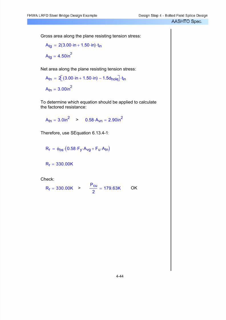
7/29/2019 LRFD steel design.pdf
http://slidepdf.com/reader/full/lrfd-steel-designpdf 243/646
OKPcu
2179.63K=>Rr 330.00K=
Check:
Rr 330.00K=
Rr φbs 0.58 Fy⋅ Avg⋅ Fu Atn⋅+( )⋅=
Therefore, use SEquation 6.13.4-1:
0.58 Avn⋅ 2.90in2=> Atn 3.0in
2=
To determine which equation should be applied to calculatethe factored resistance:
Atn 3.00in2
=
Atn 2 3.00 in⋅ 1.50 in⋅+( ) 1.5dhole− tin⋅=
Net area along the plane resisting tension stress:
Atg 4.50in2
=
Atg 2 3.00 in⋅ 1.50 in⋅+( ) tin⋅=
Gross area along the plane resisting tension stress:
4-44

7/29/2019 LRFD steel design.pdf
http://slidepdf.com/reader/full/lrfd-steel-designpdf 244/646
Girder Bottom Flange:
The girder bottom flange will now be checked for block shear. SeeFigure 4-7 for the assumed failure mode:
14.00"
3.00”
1.50”
5.00”
3.00” 3.00” 1.75"
1.00” Ø
Field
Splice
CL
Figure 4-7 Bottom Flange - Block Shear Check
Applying the factored resistance equations presented previously tothe bottom flange for the assumed failure mode:
Gross area along the plane resisting shear stress:
Avg 4 2 3.00 in⋅( )⋅ 1.75 in⋅+[ ] tflbL⋅=
Avg
27.13in2
=
Net area along the plane resisting shear stress:
Avn 4 2 3.00 in⋅( )⋅ 1.75 in⋅+[ ] 2.5 dhole⋅− tflbL⋅=
Avn 18.38in2
=
4-45

7/29/2019 LRFD steel design.pdf
http://slidepdf.com/reader/full/lrfd-steel-designpdf 245/646
It should be noted that although the block shear checks performedin this design example indicate an overdesign, the number of boltscannot be reduced prior to checking shear on the bolts andbearing at the bolt holes. These checks are performed in whatfollows.
OKPcu 359.25K=>Rr 764.19K=
Check:
Rr 764.19K=
Rr φbs 0.58 Fu⋅ Avn⋅ Fy Atg⋅+( )⋅=
Therefore, use SEquation 6.13.4-2:
0.58 Avn⋅ 10.66in2
=< Atn 3.50in2
=
To determine which equation should be applied to calculatethe factored resistance:
Atn 3.50in2
=
Atn 2 3.00 in⋅( ) 1.0dhole− tflbL⋅=
Net area along the plane resisting tension stress:
Atg 5.25in2=
Atg 2 3.00 in⋅( ) tflbL⋅=
Gross area along the plane resisting tension stress:
4-46

7/29/2019 LRFD steel design.pdf
http://slidepdf.com/reader/full/lrfd-steel-designpdf 246/646
Ns 2=Number of shear planes per bolt:
Fub 120ksi=
Fub Fubolt=Specified minimum tensile strengthof the bolt from Design Step 4.1:
Ab 0.60in2
=
Abπ
4dbolt
2⋅= Area of the bolt corresponding to the
nominal diameter:
where:
SEquation
6.13.2.7-1R
n0.48 A
b⋅ F
ub⋅ N
s⋅
( )= N
s
The nominal shear resistance is computed first as follows:
The factored resistance of an ASTM A325 7/8" diameter high-strength bolt in shear must be determined, assuming thethreads are excluded from the shear planes. For this case, thenumber of bolts required to provide adequate shear strength isdetermined by assuming the design force acts on two shear planes, known as double shear.
Pcu 459.38 K⋅=
The Strength I flange design force used in this check waspreviously computed (reference Table 4-15):
Determine the number of bolts for the bottom flange splice platesthat are required to develop the Strength I design force in the flange
in shear assuming the bolts in the connection have slipped andgone into bearing. A minimum of two rows of bolts should beprovided to ensure proper alignment and stability of the girder during construction.
Flange Bolts - Shear:
4-47

7/29/2019 LRFD steel design.pdf
http://slidepdf.com/reader/full/lrfd-steel-designpdf 247/646
γ Af
Ap=
Ap
where:
SEquation6.13.6.1.5-1
R 1 γ+( )1 2γ+( )⎡⎣ ⎤⎦
= γ
In this design example, the reduction factor approach will be used.The reduction factor per the Specifications is:
The fillers need not be extended and developed provided thatthe factored resistance of the bolts in shear at the StrengthLimit State, specified in Article 6.13.2.2, is reduced by anappropriate factor:
or
The fillers shall be extended beyond the gusset or splice materialand shall be secured by enough additional bolts to distribute thetotal stress in the member uniformly over the combined section of the member and the filler.
S6.13.6.1.5When bolts carrying loads pass through fillers 0.25 inches or more in thickness in axially loaded connections, includinggirder flange splices, either:
Ru 55.42K=
(Design Step 4.1)φs 0.80=
Ru φs Rn⋅=
The factored shear resistance now follows:
Rn 69.27K=
Rn 2 0.48 Ab⋅ Fub⋅( )⋅=
4-48

7/29/2019 LRFD steel design.pdf
http://slidepdf.com/reader/full/lrfd-steel-designpdf 248/646
γ 0.58=γ Af
Ap=
Therefore:
Ap 12.13in2=
Ap min Ap1 Ap2,( )=
The minimum of the areas is:
Ap2 12.13in2
=
Ap2 Agross_in Agross_out+=
Agross_out 6.13in2= Agross_in 6.00in2=
Sum of splice plate areas is equal to the grossareas of the inside and outside splice plates:
Ap1 12.25in2=
Ap1 bflbL( ) tflbL( )⋅=
tflbL 0.875in=
bflbL 14in=
Bottom flange area:
The smaller of either the connected plate area (i.e., girder flange)or the sum of the splice plate areas on the top and bottom of theconnected plate determines Ap.
Af 7.00in2
=
Af bfill tfill=
Sum of the area of the fillers on the top and bottomof the connected plate:
4-49
7/29/2019 LRFD steel design.pdf
http://slidepdf.com/reader/full/lrfd-steel-designpdf 249/646
SEquation
6.13.2.8-1Rn Kh Ks⋅ Ns⋅ Pt⋅= Pt
SEquation
6.13.2.2-1Rr Rn=
The factored resistance for slip-critical connections is:
Ps 184.98 K⋅=
From Table 4-17, the Service II bottom flange design force is:
C6.13.6.1.4cWhen checking for slip of the bolted connection for a flange splicewith inner and outer splice plates, the slip resistance should alwaysbe determined by dividing the flange design force equally to the twoslip planes regardless of the ratio of the splice plate areas. Slip of the connection cannot occur unless slip occurs on both planes.
S 6.13.6.1.4cBolted connections for flange splices shall be designed asslip-critical connections for the Service II flange design force, or the flange design force from constructibility, whichever governs.In this design example, the Service II flange force controls (seeprevious discussion in Design Step 4.3).
Flange Bolts - Slip Resistance:
The minimum number of bolts required on each side of the splice toresist the maximum Strength I flange design force in shear is twelve.
N 11.32=NPcu
R=
The number of bolts required per side is:
R 40.57K=
R Ru Rfill⋅=
To determine the total number of bolts required for the bottom flangesplice, divide the applied Strength I flange design force by the reducedallowable bolt shear strength:
Rfill 0.73=Rfill1 γ+( )
1 2γ+( )⎡⎣
⎤⎦
=
The reduction factor is determined to be:
4-50

7/29/2019 LRFD steel design.pdf
http://slidepdf.com/reader/full/lrfd-steel-designpdf 250/646
Friction Coeffic ient Selection
Weathering steel can be blasted for a Class B surface. Also, for painted steel, most inorganic zinc (IOZ)primers provide a Class B surface.
Therefore, the number of bolts required for the bottom-flange splice iscontrolled by the bolt shear requirements. Arrange the bolts in threerows of four bolts per line with no stagger.
12 bolts determined previously tosatisfy the bolt shear requirements.
bolts < N =N 5=
Use:
N 4.74=N
Ps
Rr =
The minimum number of bolts required to prevent slip is:
Rr 39.00K=Rr Kh Ks⋅ Ns⋅ Pt⋅=
STable 6.13.2.8-3Ks 0.50=Surface condition factor for Class B surface conditions:
STable 6.13.2.8-2Kh 1.0=Hole size factor:
STable 6.13.2.8-1Pt 39.0 K⋅=Minimum required bolt tension:
Ns 2=Number of slip planes per bolt:
Additionally:
S6.13.2.8Class B surfaces are unpainted blast-cleaned surfaces andblast-cleaned surfaces with Class B coatings.
Determine the factored resistance per bolt assuming a ClassB surface condition for the faying surface, standard holes
(which are required per S6.13.6.1.4a) and two slip planes per bolt:
4-51
7/29/2019 LRFD steel design.pdf
http://slidepdf.com/reader/full/lrfd-steel-designpdf 251/646
OKs 5.75 in⋅≤
5.75 in⋅ 7.00 in⋅≤4.0 in⋅ 4.0 tout⋅+ 5.75in=
Maximum spacing for sealing:
tout 0.4375in=Thickness of the thinner outside plate or shape:
where:
s 4.0 4.0 t⋅+( )≤ 7.0≤
For a single line adjacent to a free edge of an outside plate or shape (for example, the bolts along the edges of the plate parallelto the direction of the applied force):
The maximum spacing of the bolts is limited to prevent penetrationof moisture in the joints.
S6.13.2.6.2Flange Bolts - Maximum Spacing for Sealing:
The minimum spacing requirement is satisfied.
(see Figures 4-4 thru 4-7)s 3.00 in⋅=For this example,
smin 2.63in=
smin 3 dbolt⋅=
(Design Step 4.1)dbolt 0.875in=
The minimum spacing between centers of bolts in standard holesshall be no less than three times the diameter of the bolt.
S6.13.2.6.1Flange Bolts - Minimum Spacing:
4-52

7/29/2019 LRFD steel design.pdf
http://slidepdf.com/reader/full/lrfd-steel-designpdf 252/646
Referring to Figures 4-4 thru 4-7, it is clear that theminimum edge distance specified for this example is 1 1/2"and thus satisfies the minimum requirement.
STable 6.13.2.6.6-1For a 7/8" diameter bolt measured to a sheared edge, the
minimum edge distance is 1 1/2".
The minimum required edge distance is measured as thedistance from the center of any bolt in a standard hole to anedge of the plate.
Minimum:
S6.13.2.6.6Flange Bolts - Edge Distance:
The maximum pitch requirements are applicable only for
mechanically fastened built-up members and will not be applied inthis example.
S6.13.2.6.3Flange Bolts - Maximum Pitch for Stitch Bolts:
Therefore the requirement is satisfied.
OKsend 5.75 in⋅≤
4.00 in⋅ 4.00 tout
⋅+ 5.75in=
Maximum spacing for sealing:
send 5.00 in⋅=
Maximum spacing along the free edge at the end of the spliceplate (see Figures 4-4 thru 4-7):
s 4.00 4.00 t⋅+( )≤ 7.00≤
Next, check for sealing along the free edge at the end of thesplice plate. The bolts are not staggered, therefore theapplicable equation is:
4-53

7/29/2019 LRFD steel design.pdf
http://slidepdf.com/reader/full/lrfd-steel-designpdf 253/646
Maximum:
The maximum edge distance shall not be more than eighttimes the thickness of the thinnest outside plate or five inches.
8 t⋅ 5.00 in⋅≤
where:
t tout=
tout 0.4375in=
The maximum edge distance allowable is:
8 tout⋅ 3.50in=
The maximum distance from the corner bolts to the corner of thesplice plate or girder flange is equal to (reference Figure 4-7):
1.50 in⋅( )2
1.75 in⋅( )2+ 2.30in=
and satisfies the maximum edge distance requirement.
2.30 in⋅ 3.50 in⋅≤ OK
4-54

7/29/2019 LRFD steel design.pdf
http://slidepdf.com/reader/full/lrfd-steel-designpdf 254/646
Lc22.00in=
Lc23.00 in⋅ dhole−=
The center-to-center distance between bolts in thedirection of the force is three inches. Therefore, the clear distance between edges of adjacent holes is computed as:
Lc11.00in=
Lc11.50 in⋅
dhole
2−=
(Design Step 4.1)dhole 1.0in=
For the bolts adjacent to the end of the splice plate, theedge distance is 1 1/2". Therefore, the clear end distancebetween the edge of the hole and the end of the splice plate:
2 dbolt⋅ 1.75in=
(Design Step 4.1)dbolt 0.875in=
To determine the applicable equation for the calculation of the nominalresistance, the clear distance between holes and the clear enddistance must be calculated and compared to the value of two timesthe nominal diameter of the bolt. This check yields:
The element of the bottom flange splice that controls the bearingcheck in this design example is the outer splice plate.
The design bearing strength of the connected material is calculated asthe sum of the bearing strengths of the individual bolt holes parallel tothe line of the applied force.
Pcu 459.38 K⋅=
Check bearing of the bolts on the connected material under themaximum Strength I Limit State design force. The maximum
Strength I bottom flange design force from Table 4-15 is:
S6.13.2.9Flange Bolts - Bearing at Bolt Holes:
4-55

7/29/2019 LRFD steel design.pdf
http://slidepdf.com/reader/full/lrfd-steel-designpdf 255/646
OKRr 546.00K=<Pcu
2229.69K=
Check:
Rr 546.00K=
Rr φbb Rn⋅=
(Design Step 4.1)φbb 0.80=
Rn 682.50K=
Rn Rn1Rn2
+=
The total nominal resistance of the bolt holes is:
Rn2546.00K=
Rn28 1.2 Lc2
⋅ tout⋅ Fu⋅( )⋅=
The nominal resistance for the remaining bolt holes is computedas follows:
Rn1136.50K=
Rn14 1.2 Lc1
⋅ tout⋅ Fu⋅( )⋅=
The nominal resistance for the end row of bolt holes is computedas follows:
Fu 65ksi=Tensile strength of the connected material(Design Step 4.1):
tout 0.4375in=Thickness of the connected material:
For the outside splice plate:
SEquation
6.13.2.9-2
Rn 1.2 Lc⋅ t⋅ Fu⋅=
For standard holes, where either the clear distance between holesor the clear end distance is less than twice the bolt diameter:
4-56

7/29/2019 LRFD steel design.pdf
http://slidepdf.com/reader/full/lrfd-steel-designpdf 256/646
STable
6.6.1.2.3-1
The fatigue detail category under the condition of Mechanically Fastened Connections for checking thebase metal at the gross section of high-strength boltedslip-resistant connections is Category B.
SEquation
6.6.1.2.5-1∆F
n
A
N
⎛
⎝
⎞
⎠
1
31
2∆F
TH⋅≥= ∆F
TH
∆F( )n
Nominal fatigue resistance:
γ ∆f ( ) ∆f fact=
Force effect, live load stress range due to the passage of the fatigue load:
γ 0.75=Load factor for the fatigue load combination:
where:
SEquation
6.6.1.2.2-1γ ∆f ( )⋅ ∆F( )
n≤
For load-induced fatigue considerations, each detail shall satisfy:
∆f fact 4.63 ksi⋅=
From Table 4-18, the factored fatigue stress range at themidthickness of the bottom flange is:
Check the fatigue stresses in the base metal of the bottom flangesplice plates adjacent to the slip-critical connections. Fatigue
normally does not govern the design of the splice plates, andtherefore, an explicit check is not specified. However, a fatiguecheck of the splice plates is recommended whenever thecombined area of the inside and outside flange splice plates isless than the area of the smaller flange at the splice.
S6.6.1Fatigue of Splice Plates:
4-57
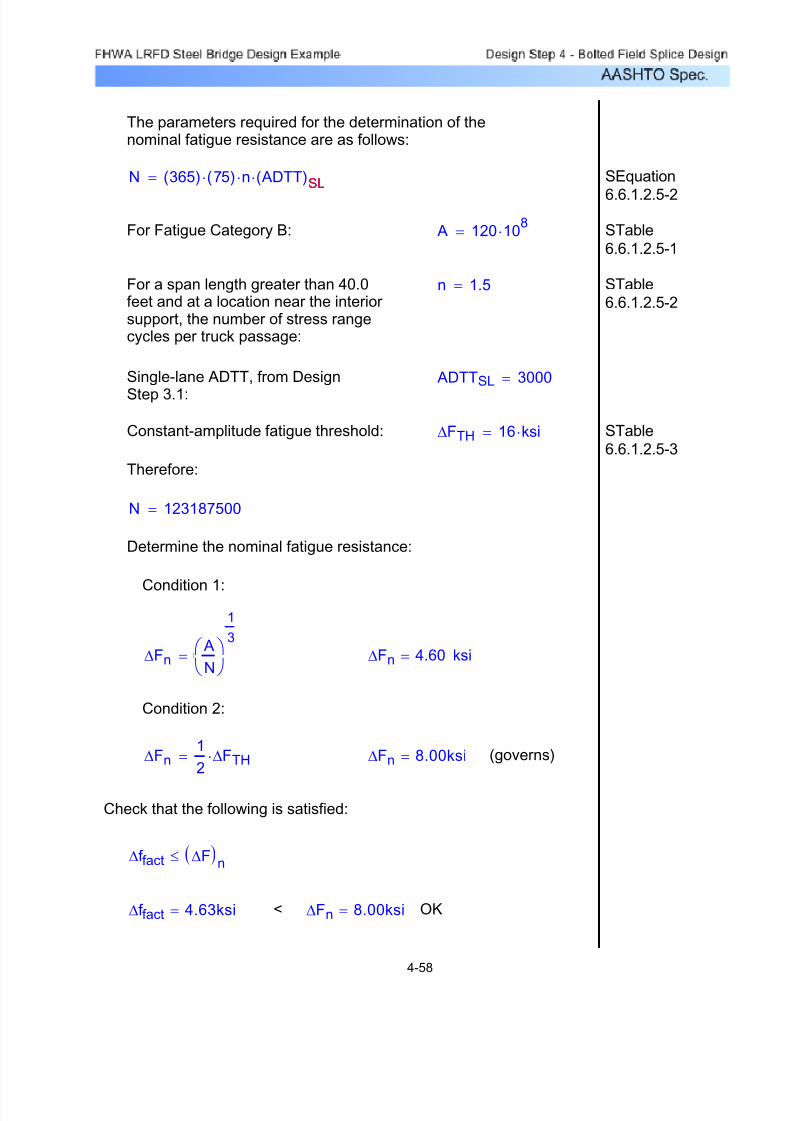
7/29/2019 LRFD steel design.pdf
http://slidepdf.com/reader/full/lrfd-steel-designpdf 257/646
OK∆Fn 8.00ksi=<∆f fact 4.63ksi=
∆f fact ∆F( )n
≤
Check that the following is satisfied:
(governs)∆Fn 8.00ksi=∆Fn1
2∆FTH⋅=
Condition 2:
ksi∆Fn 4.60=∆Fn A
N
⎛ ⎝
⎞ ⎠
1
3
=
Condition 1:
Determine the nominal fatigue resistance:
N 123187500=
Therefore:
STable
6.6.1.2.5-3∆FTH 16 ksi⋅=Constant-amplitude fatigue threshold:
ADTTSL 3000=Single-lane ADTT, from Design
Step 3.1:
STable
6.6.1.2.5-2n 1.5=For a span length greater than 40.0
feet and at a location near the interior support, the number of stress rangecycles per truck passage:
STable
6.6.1.2.5-1 A 120 10
8⋅=For Fatigue Category B:
SEquation
6.6.1.2.5-2
N 365( ) 75( )⋅ n⋅ ADTT( )SL⋅= SL
The parameters required for the determination of thenominal fatigue resistance are as follows:
4-58

7/29/2019 LRFD steel design.pdf
http://slidepdf.com/reader/full/lrfd-steel-designpdf 258/646
OK0.95 Fyf ⋅ 47.50ksi=<f_out 15.10ksi=
f_out 15.10ksi=f_outP
Agross_out=
Agross_out 6.13in2=
The resulting stress in the outside splice plate is:
P 92.49K=PPs
2=
The flange force is equally distributed to the inner and outer spliceplates due to the areas of the flanges being within 10 percent of eachother:
Fyf 50ksi=Specified minimum yield strengthof the flange (Design Step 4.1):
f f Elastic flange stress causedby the factored loading:
where:
SEquation
6.10.5.2-1f f 0.95 Fyf ⋅≤
The following criteria will be used to make this check. The equation
presented is for both steel flanges of composite section:
Ps 184.98K=
The maximum Service II flange force in the bottom flange is takenfrom Table 4-17:
A check of the flexural stresses in the splice plates at the Service IILimit State is not explicitly specified in the specifications. However,
whenever the combined area of the inside and outside flange spliceplates is less than the area of the smaller flange at the splice (which isthe case for the bottom flange splice in this example), such a check isrecommended.
S6.10.5.2Control of Permanent Deflection - Splice Plates:
4-59

7/29/2019 LRFD steel design.pdf
http://slidepdf.com/reader/full/lrfd-steel-designpdf 259/646
The resulting stress in the inside splice plates is:
Agross_in 6.00in2
=
f_inP
Agross_in= f_in 15.42ksi=
f_in 15.42ksi= < 0.95 Fyf ⋅ 47.50ksi= OK
Design Step 4.5 - Design Top Flange Splice
The design of the top flange splice is not included in this designexample (for the sake of simplicity and brevity). However, the topflange splice is designed using the same procedures and methodspresented in this design example for the bottom flange splice.
4-60
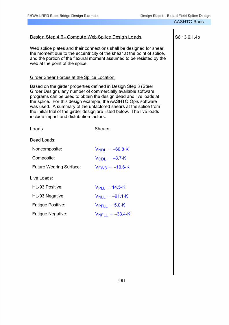
7/29/2019 LRFD steel design.pdf
http://slidepdf.com/reader/full/lrfd-steel-designpdf 260/646
VNFLL 33.4− K⋅=Fatigue Negative:
VPFLL 5.0 K⋅=Fatigue Positive:
VNLL 91.1− K⋅=HL-93 Negative:
VPLL 14.5 K⋅=HL-93 Positive:
Live Loads:
VFWS 10.6− K⋅=Future Wearing Surface:
VCDL 8.7− K⋅=Composite:
VNDL 60.8− K⋅=Noncomposite:
Dead Loads:
ShearsLoads
Based on the girder properties defined in Design Step 3 (SteelGirder Design), any number of commercially available softwareprograms can be used to obtain the design dead and live loads atthe splice. For this design example, the AASHTO Opis softwarewas used. A summary of the unfactored shears at the splice from
the initial trial of the girder design are listed below. The live loadsinclude impact and distribution factors.
Girder Shear Forces at the Splice Location:
Web splice plates and their connections shall be designed for shear,the moment due to the eccentricity of the shear at the point of splice,
and the portion of the flexural moment assumed to be resisted by theweb at the point of the splice.
S6.13.6.1.4bDesign Step 4.6 - Compute Web Splice Design Loads
4-61

7/29/2019 LRFD steel design.pdf
http://slidepdf.com/reader/full/lrfd-steel-designpdf 261/646
Web Moments and Horizontal Force Resultant: C6.13.6.1.4b
Because the portion of the flexural moment assumed to be resistedby the web is to be applied at the mid-depth of the web, a horizontal
design force resultant, Huw, must also be applied at the mid-depth of the web to maintain equilibrium. The web moment and horizontalforce resultant are applied together to yield a combined stressdistribution equivalent to the unsymmetrical stress distribution in theweb. For sections with equal compressive and tensile stresses at thetop and bottom of the web (i.e., with the neutral axis located at themid-depth of the web), Huw will equal zero.
In the computation of the portion of the flexural moment assumedto be resisted by the web, Muw, and the horizontal design forceresultant, Huw, in the web, the flange stresses at the midthickness
of the flanges are conservatively used. This allows use of thesame stress values for both the flange and web splices, whichsimplifies the calculations. It is important to note that the flangestresses are taken as signed quantities in determining Muw andHuw (positive for tension; negative for compression).
C6.13.6.1.4b
The moment, Muv, due to the eccentricity of the design shear, Vuw,is resisted solely by the web and always acts about the mid-depthof the web (i.e., horizontal force resultant is zero). This moment iscomputed as:
Muv Vuw e⋅= Vuw
where e is defined as the distance from the centerline of thesplice to the centroid of the connection on the side of the jointunder consideration. For this design example:
S6.13.6.1.4b
e 1.9375 in⋅3.00 in⋅
2+= (Reference Figure 4-8)
e 3.44in=
The total web moment for each load case is computed as follows:
Mtotal Muw Muv+= Muv
In general, and in this example, the web splice is designed under the conservative assumption that the maximum moment andshear at the splice will occur under the same loading condition.
4-62

7/29/2019 LRFD steel design.pdf
http://slidepdf.com/reader/full/lrfd-steel-designpdf 262/646
tw 0.50in=Thickness of the web:
D 54 in=Web Depth:
From Figure 4-1:
Fyw 50ksi=
Fyw Fy=Specified minimum
yield strength of the web(Design Step 4.1):
E 29000 ksi⋅=Modulus of Elasticity:
S6.10.7.2k 5.0=
And:
1.38E k⋅Fyw⋅and1.10
E k⋅Fyw⋅
Strength I Limit State:
Design Shear: S6.13.6.1.4b
For the Strength I Limit State, the girder web factored shear resistance is required when determining the design shear. Assumean unstiffened web at the splice location. S6.10.7.2
φv 1.00= (Design Step 4.1)
Vr φv Vn⋅= Vn SEquation
6.10.7.1-1
Vn C Vp⋅= Vp SEquation
6.10.7.2-1
Vp 0.58 Fyw⋅ D⋅ tw⋅= Fyw SEquation
6.10.7.2-2
where:
Ratio of shear buckling stress to the shear yield strength, C,is dependent upon the ratio of D/tw in comparison to:
S6.10.7.3.3a
4-63
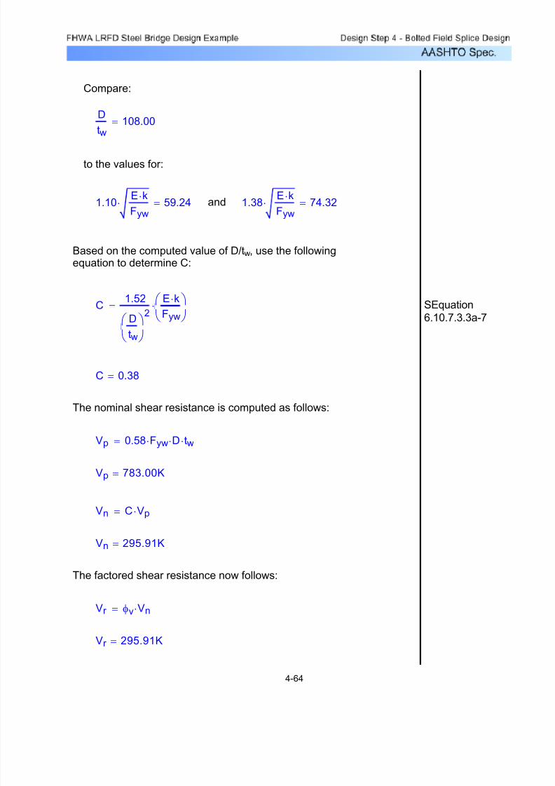
7/29/2019 LRFD steel design.pdf
http://slidepdf.com/reader/full/lrfd-steel-designpdf 263/646
Vr 295.91K=
Vr φv Vn⋅=
The factored shear resistance now follows:
Vn
295.91K=
Vn C Vp⋅=
Vp 783.00K=
Vp 0.58 Fyw⋅ D⋅ tw⋅=
The nominal shear resistance is computed as follows:
C 0.38=
SEquation
6.10.7.3.3a-7C
1.52
D
tw
⎛ ⎝
⎞ ⎠
2
E k⋅Fyw
⎛ ⎝
⎞ ⎠
⋅=
Based on the computed value of D/tw, use the followingequation to determine C:
1.38E k⋅Fyw
⋅ 74.32=and1.10E k⋅Fyw
⋅ 59.24=
to the values for:
D
tw
108.00=
Compare:
4-64
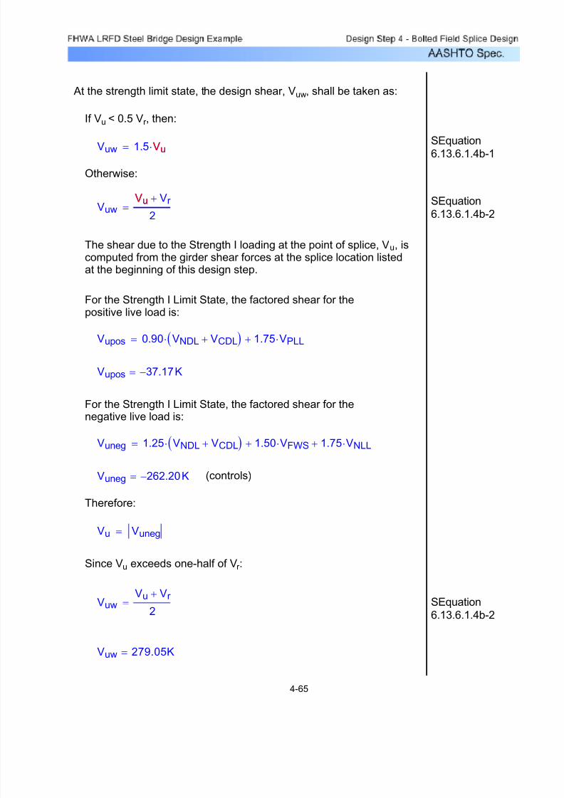
7/29/2019 LRFD steel design.pdf
http://slidepdf.com/reader/full/lrfd-steel-designpdf 264/646
Vuw 279.05K=
SEquation
6.13.6.1.4b-2Vuw
Vu Vr +
2=
Since Vu exceeds one-half of Vr :
Vu Vuneg=
Therefore:
(controls)Vuneg 262.20− K=
Vuneg 1.25 VNDL VCDL+( )⋅ 1.50 VFWS⋅+ 1.75 VNLL⋅+=
For the Strength I Limit State, the factored shear for the
negative live load is:
Vupos 37.17− K=
Vupos 0.90 VNDL VCDL+( )⋅ 1.75 VPLL⋅+=
For the Strength I Limit State, the factored shear for thepositive live load is:
The shear due to the Strength I loading at the point of splice, Vu, iscomputed from the girder shear forces at the splice location listedat the beginning of this design step.
VuwVu Vr +
2=
Vu SEquation
6.13.6.1.4b-2
Otherwise:
Vuw 1.5 Vu⋅= Vu SEquation6.13.6.1.4b-1
If Vu < 0.5 Vr , then:
At the strength limit state, the design shear, Vuw, shall be taken as:
4-65

7/29/2019 LRFD steel design.pdf
http://slidepdf.com/reader/full/lrfd-steel-designpdf 265/646
D 54 in=Web depth:
tw 0.50in=Web thickness:
Rcf 1.60=Rcf Fcf
f cf =
The ratio Rcf is computed as follows:
Rh 1.00=The hybrid girder reduction factor:
where:
CEquation
6.13.6.1.4b-1Mw
tw D2⋅
12Rh Fcf ⋅ Rcf f ncf ⋅−⋅=
Therefore, the portion of the flexural moment assumed to beresisted by the web is computed as:
f ncf 0.93− ksi⋅=
For the same loading condition, the concurrent flexural stress atthe midthickness of the noncontrolling (top) flange, f ncu, waspreviously computed. From Table 4-16:
Fcf 37.50 ksi⋅=
f cf 23.48 ksi⋅=
For the loading condition with positive live load, the controllingflange was previously determined to be the bottom flange. Themaximum elastic flexural stress due to the factored loads at themidthickness of the controlling flange, f cf , and the design stressfor the controlling flange, Fcf , were previously computed for thisloading condition. From Table 4-15:
Case 1 - Dead Load + Positive Live Load:
Web Moments and Horizontal Force Resultants:
4-66

7/29/2019 LRFD steel design.pdf
http://slidepdf.com/reader/full/lrfd-steel-designpdf 266/646
Compute the portion of the flexural moment to beresisted by the web:
Mw_str_postw D2⋅
12Rh Fcf ⋅ Rcf f ncf ⋅−⋅ 1
12in
ft
⎛
⎝
⎞
⎠
⋅=
Mw_str_pos 394.73K ft⋅=
The total web moment is:
Vuw 279.05K= e 3.44 in=
Mtot_str_pos Mw_str_pos Vuw e⋅( ) 1
12in
ft
⎛
⎝
⎞
⎠
⋅+=
Mtot_str_pos 474.66K ft⋅=
Compute the horizontal force resultant (the variables includedin this equation are as defined for Mw_str_pos):
Hw_str_postw D⋅
2Rh Fcf ⋅ Rcf f ncf ⋅+( )⋅= CEquation
6.13.6.1.4b-2
Hw_str_pos 486.20K=
The above value is a signed quantity, positive for tension andnegative for compression.
4-67
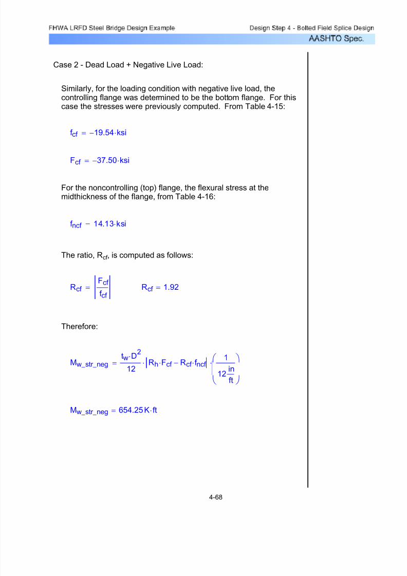
7/29/2019 LRFD steel design.pdf
http://slidepdf.com/reader/full/lrfd-steel-designpdf 267/646
Case 2 - Dead Load + Negative Live Load:
Similarly, for the loading condition with negative live load, the
controlling flange was determined to be the bottom flange. For thiscase the stresses were previously computed. From Table 4-15:
f cf 19.54− ksi⋅=
Fcf 37.50− ksi⋅=
For the noncontrolling (top) flange, the flexural stress at themidthickness of the flange, from Table 4-16:
f ncf 14.13 ksi⋅=
The ratio, Rcf , is computed as follows:
Rcf Fcf
f cf = Rcf 1.92=
Therefore:
Mw_str_negtw D
2⋅
12Rh Fcf ⋅ Rcf f ncf ⋅−⋅
1
12in
ft
⎛
⎝
⎞
⎠
⋅=
Mw_str_neg 654.25K ft⋅=
4-68

7/29/2019 LRFD steel design.pdf
http://slidepdf.com/reader/full/lrfd-steel-designpdf 268/646
The total web moment is:
Vuw 279.05K= e 3.44 in=
Mtot_str_neg Mw_str_neg Vuw e⋅( )1
12in
ft
⎛
⎝
⎞
⎠
⋅+=
Mtot_str_neg 734.19K ft⋅=
Compute the horizontal force resultant:
Hw_str_negtw D⋅
2Rh Fcf ⋅ Rcf f ncf ⋅+( )⋅=
Hw_str_neg 140.16− K=
The above value is a signed quantity, positive for tension, andnegative for compression.
4-69

7/29/2019 LRFD steel design.pdf
http://slidepdf.com/reader/full/lrfd-steel-designpdf 269/646
Service II Limit State:
Design Shear:
As a minimum, for checking slip of the web splice bolts, thedesign shear shall be taken as the shear at the point of spliceunder the Service II Limit State, or the shear from constructibility,whichever governs. In this design example, the Service II shear controls (see previous discussion in Design Step 4.3).
S6.13.6.1.4b
The elastic shears due to the unfactored loads at the point of the splice are listed at the beginning of this design step.
For the Service II Limit State, the factored shear for thepositive live load is (ignore future wearing surface):
Vser_pos 1.00 VNDL⋅ 1.00 VCDL⋅+ 1.30 VPLL⋅+=
Vser_pos 50.65− K=
For the Service II Limit State, the factored shear for thenegative live load is (include future wearing surface):
Vser_neg 1.00 VNDL⋅ 1.00 VCDL⋅+ 1.00 VFWS⋅+ 1.30 VNLL⋅+=
Vser_neg 198.53− K= (governs)
Therefore:
Vw_ser Vser_neg=
4-70
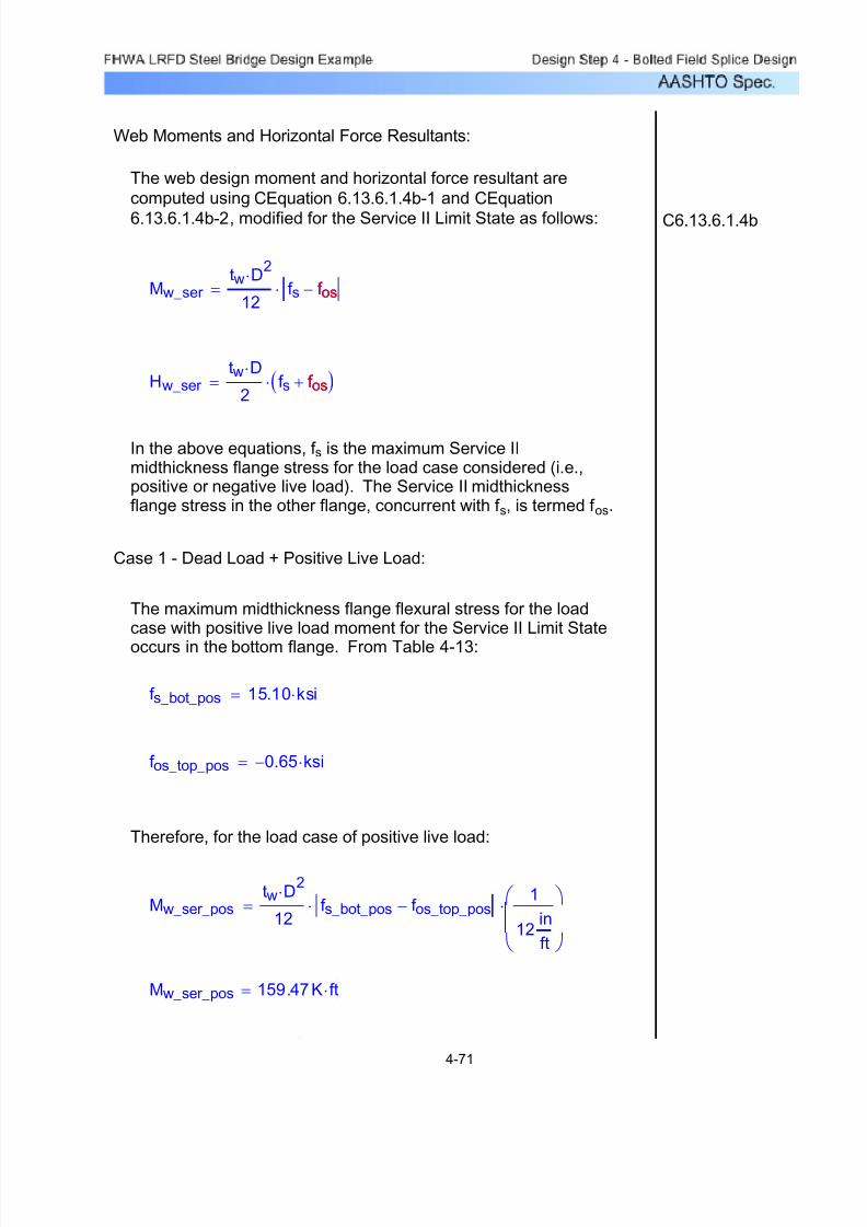
7/29/2019 LRFD steel design.pdf
http://slidepdf.com/reader/full/lrfd-steel-designpdf 270/646
Web Moments and Horizontal Force Resultants:
The web design moment and horizontal force resultant are
computed using CEquation 6.13.6.1.4b-1 and CEquation
6.13.6.1.4b-2, modified for the Service II Limit State as follows: C6.13.6.1.4b
Mw_ser tw D
2⋅
12f s f os−⋅= f os
Hw_ser tw D⋅
2f s f os+( )⋅= f os
In the above equations, f s is the maximum Service IImidthickness flange stress for the load case considered (i.e.,positive or negative live load). The Service II midthicknessflange stress in the other flange, concurrent with f s, is termed f os.
Case 1 - Dead Load + Positive Live Load:
The maximum midthickness flange flexural stress for the loadcase with positive live load moment for the Service II Limit State
occurs in the bottom flange. From Table 4-13:
f s_bot_pos 15.10 ksi⋅=
f os_top_pos 0.65− ksi⋅=
Therefore, for the load case of positive live load:
Mw_ser_postw D
2⋅
12f s_bot_pos f os_top_pos−⋅
1
12in
ft
⎛
⎝
⎞
⎠
⋅=
Mw_ser_pos 159.47K ft⋅=
4-71
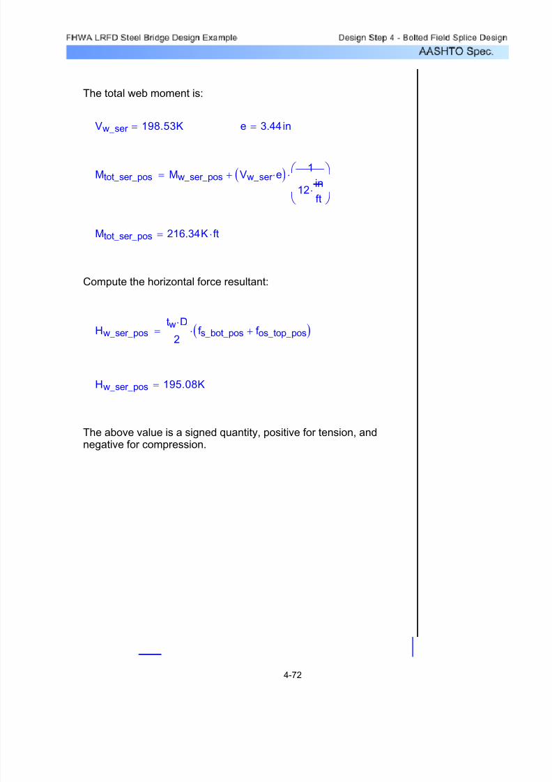
7/29/2019 LRFD steel design.pdf
http://slidepdf.com/reader/full/lrfd-steel-designpdf 271/646
The total web moment is:
Vw_ser 198.53K= e 3.44in=
Mtot_ser_pos Mw_ser_pos Vw_ser e⋅( )1
12in
ft⋅
⎛
⎝
⎞
⎠
⋅+=
Mtot_ser_pos 216.34K ft⋅=
Compute the horizontal force resultant:
Hw_ser_postw D⋅
2f s_bot_pos f os_top_pos+( )⋅=
Hw_ser_pos 195.08K=
The above value is a signed quantity, positive for tension, andnegative for compression.
4-72

7/29/2019 LRFD steel design.pdf
http://slidepdf.com/reader/full/lrfd-steel-designpdf 272/646
The above value is a signed quantity, positive for tension, andnegative for compression.
Hw_ser_neg 135.68− K=
Hw_ser_negtw D⋅
2f s_bot_neg f os_top_neg+( )⋅=
Compute the horizontal force resultant:
Mtot_ser_neg 195.08K ft⋅=
Mtot_ser_neg Mw_ser_neg Vw_ser e⋅( ) 1
12in
ft⋅
⎛
⎝
⎞
⎠
⋅+=
e 3.44in=Vw_ser 198.53K=
The total web moment is:
Mw_ser_neg 138.21K ft⋅=
Mw_ser_neg
tw D2⋅
12 f s_bot_neg f os_top_neg−⋅1
12in
ft
⎛ ⎝
⎞ ⎠
⋅=
Therefore:
f os_top_neg 1.80 ksi⋅=
f s_bot_neg 11.85− ksi⋅=
The maximum midthickness flange flexural stress for the loadcase with negative live load moment for the Service II Limit
State occurs in the bottom flange. From Table 4-13:
Case 2 - Dead Load + Negative Live Load:
4-73
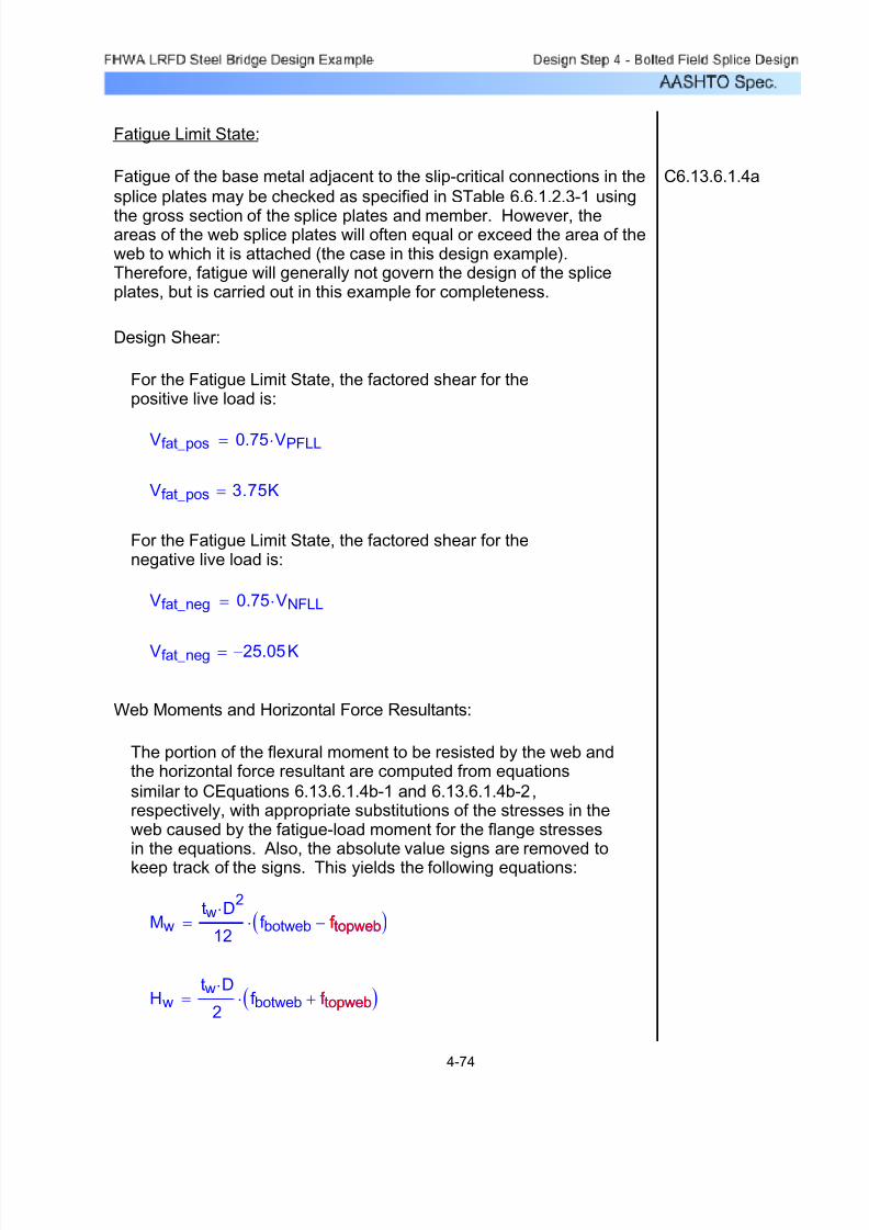
7/29/2019 LRFD steel design.pdf
http://slidepdf.com/reader/full/lrfd-steel-designpdf 273/646
7/29/2019 LRFD steel design.pdf
http://slidepdf.com/reader/full/lrfd-steel-designpdf 274/646
The above value is a signed quantity, positive for tension, andnegative for compression.
Hw_fat_pos 33.08K=
Hw_fat_postw D⋅
2
f botweb_pos f topweb_pos+( )⋅=
Compute the horizontal force resultant:
Mtot_fat_pos 30.34K ft⋅=
Mtot_fat_pos Mw_fat_pos Vfat_pos e⋅( )1
12in
ft⋅
⎛ ⎝
⎞ ⎠
⋅+=
e 3.44in=Vfat_pos 3.75K=
The total web moment is:
Mw_fat_pos 29.26K ft⋅=
Mw_fat_postw D
2⋅
12f botweb_pos f topweb_pos−( )⋅
1
12in
ft
⎛
⎝
⎞
⎠
⋅=
Therefore:
f botweb_pos 2.67 ksi⋅=
f topweb_pos 0.22− ksi⋅=
The factored stresses due to the positive live load moment for the Fatigue Limit State at the top and bottom of the web, from
Table 4-14, are:
Case 1 - Positive Live Load:
4-75
7/29/2019 LRFD steel design.pdf
http://slidepdf.com/reader/full/lrfd-steel-designpdf 275/646
The above value is a signed quantity, positive for tension, andnegative for compression.
Hw_fat_neg 23.76− K=
Hw_fat_negtw D⋅
2f botweb_neg f topweb_neg+( )⋅=
Compute the horizontal force resultant:
Mtot_fat_neg 28.24− K ft⋅=
Mtot_fat_neg Mw_fat_neg Vfat_neg e⋅( ) 1
12in
ft⋅
⎛
⎝
⎞
⎠
⋅+=
e 3.44in=Vfat_neg 25.05− K=
The total web moment is:
Mw_fat_neg 21.06− K ft⋅=
Mw_fat_neg
tw D2⋅
12 f botweb_neg f topweb_neg−( )⋅
1
12in
ft
⎛
⎝
⎞
⎠⋅=
Therefore:
f topweb_neg 0.16 ksi⋅=
f botweb_neg 1.92− ksi⋅=
The factored stresses due to the negative live load moment for the Fatigue Limit State at the top and bottom of the web, from
Table 4-14, are:
Case 2 - Negative Live Load:
4-76
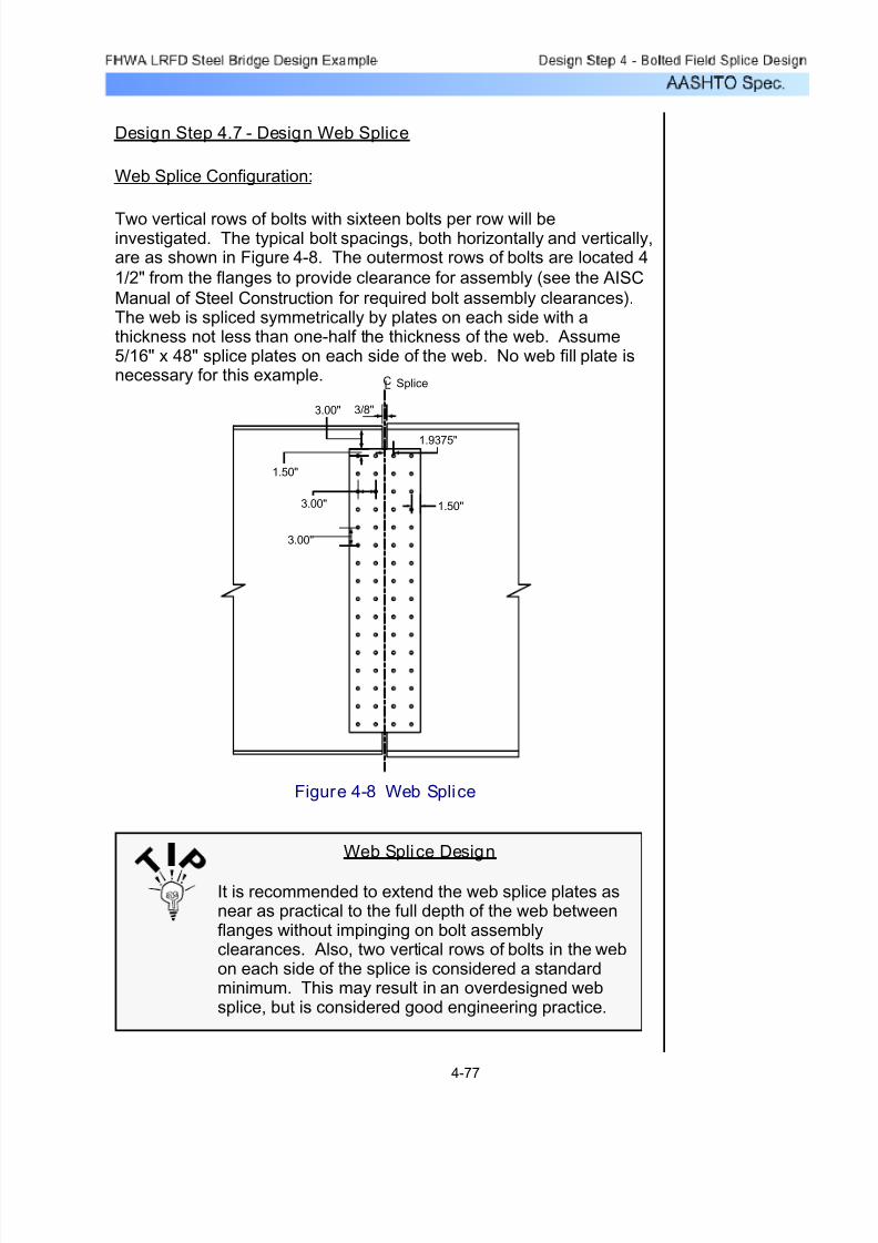
7/29/2019 LRFD steel design.pdf
http://slidepdf.com/reader/full/lrfd-steel-designpdf 276/646
Design Step 4.7 - Design Web Splice
Web Splice Configuration:
Two vertical rows of bolts with sixteen bolts per row will beinvestigated. The typical bolt spacings, both horizontally and vertically,are as shown in Figure 4-8. The outermost rows of bolts are located 4
1/2" from the flanges to provide clearance for assembly (see the AISC
Manual of Steel Construction for required bolt assembly clearances).The web is spliced symmetrically by plates on each side with athickness not less than one-half the thickness of the web. Assume5/16" x 48" splice plates on each side of the web. No web fill plate isnecessary for this example.
1.50"
3.00"
3.00"
3.00"
3/8"
1.50"
CL Splice
1.9375"
Figure 4-8 Web Splice
Web Splice Design
It is recommended to extend the web splice plates asnear as practical to the full depth of the web betweenflanges without impinging on bolt assemblyclearances. Also, two vertical rows of bolts in the webon each side of the splice is considered a standardminimum. This may result in an overdesigned websplice, but is considered good engineering practice.
4-77

7/29/2019 LRFD steel design.pdf
http://slidepdf.com/reader/full/lrfd-steel-designpdf 277/646
The maximum pitch requirements are applicable only for mechanically fastened built-up members and will not be applied inthis example.
Web Bolts - Maximum Pitch for Stitch Bolts:S6.13.2.6.3
OK3.0 in⋅ 5.25 in⋅≤
5.25 in⋅ 7.00 in⋅≤4.0 in⋅ 4.0 twp⋅+ 5.25in=
Maximum spacing for sealing:
twp 0.3125 in⋅=Thickness of the thinner outside plateor shape, in this case the web plate:
where:
s 4.0 4.0 t⋅+( )≤ 7.0≤
For a single line adjacent to a free edge of an outside plate or shape (for example, the bolts along the edges of the plate parallelto the direction of the applied force):
The maximum spacing of the bolts is limited to prevent penetrationof moisture in the joints.
S6.13.2.6.2Web Bolts - Maximum Spacing for Sealing:
This check is only dependent upon the bolt diameter, and is thereforesatisfied for a three inch spacing per the check for the flange boltsfrom Design Step 4.4.
S6.13.2.6.1Web Bolts - Minimum Spacing:
4-78
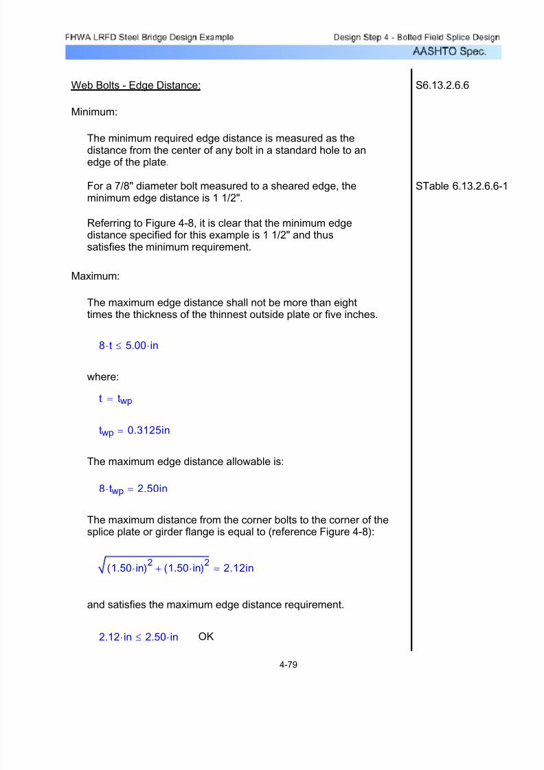
7/29/2019 LRFD steel design.pdf
http://slidepdf.com/reader/full/lrfd-steel-designpdf 278/646
OK2.12 in⋅ 2.50 in⋅≤
and satisfies the maximum edge distance requirement.
1.50 in⋅( )2
1.50 in⋅( )2
+ 2.12in=
The maximum distance from the corner bolts to the corner of thesplice plate or girder flange is equal to (reference Figure 4-8):
8 twp⋅ 2.50in=
The maximum edge distance allowable is:
twp 0.3125in=
t twp
=
where:
8 t⋅ 5.00 in⋅≤
The maximum edge distance shall not be more than eighttimes the thickness of the thinnest outside plate or five inches.
Maximum:
Referring to Figure 4-8, it is clear that the minimum edgedistance specified for this example is 1 1/2" and thussatisfies the minimum requirement.
STable 6.13.2.6.6-1For a 7/8" diameter bolt measured to a sheared edge, theminimum edge distance is 1 1/2".
The minimum required edge distance is measured as thedistance from the center of any bolt in a standard hole to anedge of the plate.
Minimum:
S6.13.2.6.6Web Bolts - Edge Distance:
4-79

7/29/2019 LRFD steel design.pdf
http://slidepdf.com/reader/full/lrfd-steel-designpdf 279/646
Ru 55.42K=
Under the most critical combination of the minimum design shear,moment and horizontal force, it is assumed that the bolts in the websplice have slipped and gone into bearing. The shear strength of an
ASTM A325 7/8" diameter high-strength bolt in double shear,assuming the threads are excluded from the shear planes, wascomputed in Design Step 4.4 for Flange Bolts - Shear:
Strength I Limit State:
Nb 32=
The total number of web bolts on each side of the splice,assuming two vertical rows per side with sixteen bolts per row, is:
Ip 6192.00in2=
Ipn m⋅12
s2
n2
1−( )⋅ g2
m2
1−( )⋅+=
The polar moment of inertia is:
g 3.00 in⋅=Horizontal pitch:
s 3.00 in⋅=Vertical pitch:
n 16=Number of bolts in one vertical row:
m 2=Number of vertical rows of bolts:
where:
CEquation
6.13.6.1.4b-3Ip
n m⋅12
s2
n2
1−( )⋅ g2
m2
1−( )⋅+= m2
1−
Calculate the polar moment of inertia, Ip, of the bolt group on each sideof the centerline with respect to the centroid of the connection. This isrequired for determination of the shear force in a given bolt due to the
applied web moments.
Web Bolts - Shear:
4-80
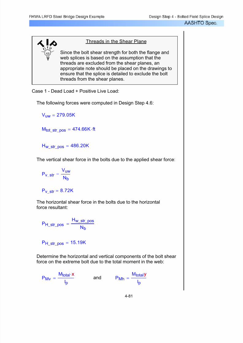
7/29/2019 LRFD steel design.pdf
http://slidepdf.com/reader/full/lrfd-steel-designpdf 280/646
PMhMtotaly
Ip=
yandPMv
Mtotal x⋅
Ip=
x
Determine the horizontal and vertical components of the bolt shear force on the extreme bolt due to the total moment in the web:
PH_str_pos 15.19K=
PH_str_posHw_str_pos
Nb=
The horizontal shear force in the bolts due to the horizontalforce resultant:
Pv_str 8.72K=
Pv_str Vuw
Nb
=
The vertical shear force in the bolts due to the applied shear force:
Hw_str_pos 486.20K=
Mtot_str_pos 474.66K ft⋅=
Vuw 279.05K=
The following forces were computed in Design Step 4.6:
Case 1 - Dead Load + Positive Live Load:
Threads in the Shear Plane
Since the bolt shear strength for both the flange and
web splices is based on the assumption that thethreads are excluded from the shear planes, anappropriate note should be placed on the drawings toensure that the splice is detailed to exclude the boltthreads from the shear planes.
4-81
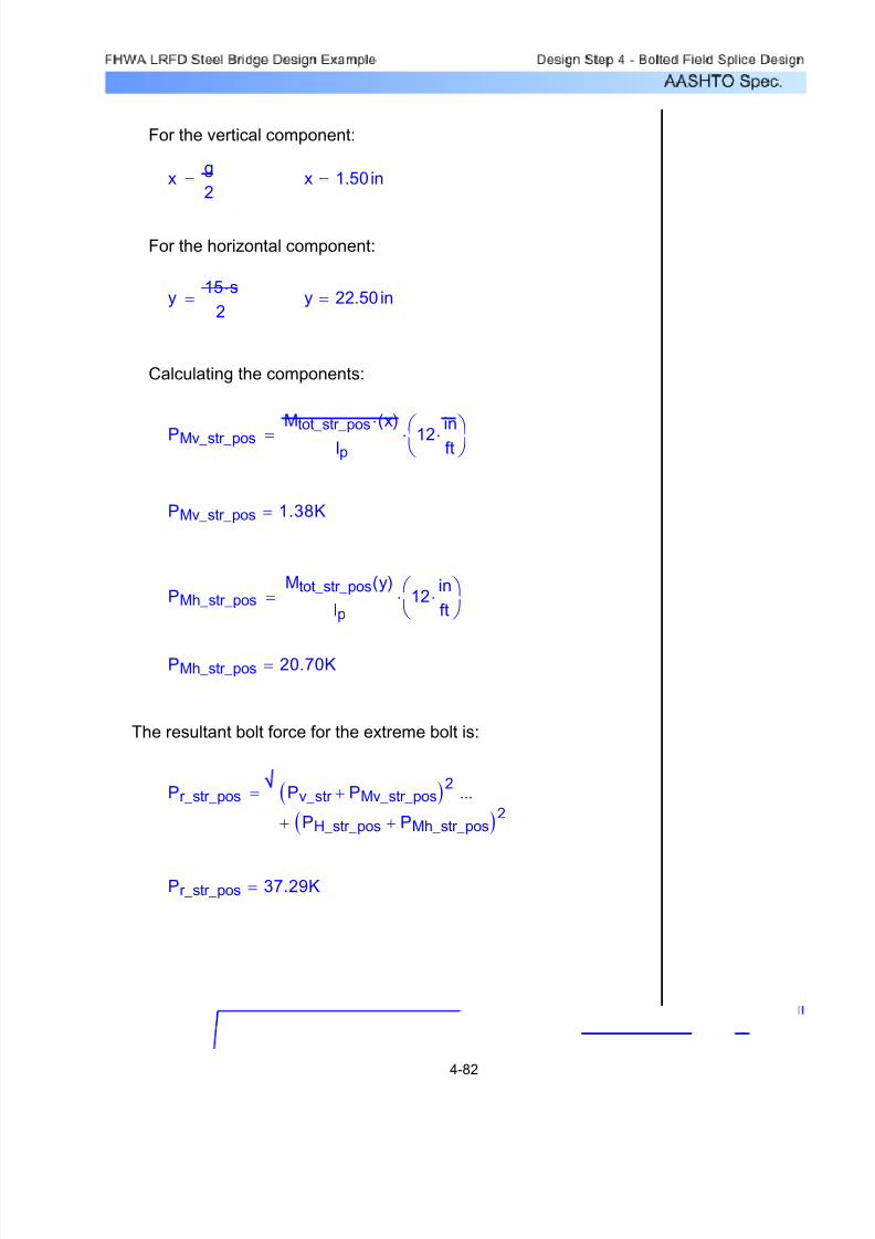
7/29/2019 LRFD steel design.pdf
http://slidepdf.com/reader/full/lrfd-steel-designpdf 281/646
For the vertical component:
xg
2= x 1.50in=
For the horizontal component:
y15 s⋅
2= y 22.50 in=
Calculating the components:
PMv_str_pos
Mtot_str_pos x( )⋅
Ip12
in
ft⋅⎛ ⎝ ⎞ ⎠⋅=
PMv_str_pos 1.38K=
PMh_str_posMtot_str_pos y( )
Ip12
in
ft⋅⎛
⎝ ⎞ ⎠
⋅=
PMh_str_pos 20.70K=
The resultant bolt force for the extreme bolt is:
Pr_str_pos Pv_str PMv_str_pos+( )2
PH_str_pos PMh_str_pos+( )2+
...=
Pr_str_pos 37.29K=
4-82

7/29/2019 LRFD steel design.pdf
http://slidepdf.com/reader/full/lrfd-steel-designpdf 282/646
Case 2 - Dead Load + Negative Live Load:
The following forces were computed in Design Step 4.6:
Vuw 279.05K=
Mtot_str_neg 734.19K ft⋅=
Hw_str_neg 140.16− K=
The vertical shear force in the bolts due to the applied shear force:
Pv_str Vuw
Nb=
Pv_str 8.72K=
The horizontal shear force in the bolts due to the horizontalforce resultant:
PH_str_negHw_str_neg
Nb=
PH_str_neg 4.38K=
Determine the horizontal and vertical components of the boltshear force on the extreme bolt due to the total moment in the web:
Calculating the components:
PMv_str_negMtot_str_neg x( )⋅
Ip12
in
ft⋅⎛
⎝ ⎞ ⎠
⋅=
PMv_str_neg 2.13K=
4-83

7/29/2019 LRFD steel design.pdf
http://slidepdf.com/reader/full/lrfd-steel-designpdf 283/646
PMh_str_negMtot_str_neg y( )
Ip12
in
ft⋅⎛
⎝ ⎞ ⎠
⋅=
PMh_str_neg 32.01K=
The resultant bolt force is:
Pr_str_neg Pv_str PMv_str_neg+( )2
PH_str_neg PMh_str_neg+( )2+
...=
Pr_str_neg 37.98K=
The governing resultant bolt force is:
Pr_str max Pr_str_pos Pr_str_neg,( )=
Pr_str 37.98K=
Check:
Pr_str 37.98K= < Ru 55.42K= OK
4-84

7/29/2019 LRFD steel design.pdf
http://slidepdf.com/reader/full/lrfd-steel-designpdf 284/646
Service II Limit State:
The factored slip resistance, Rr , for a 7/8" diameter
high-strength bolt in double shear for a Class B surface andstandard holes was determined from Design Step 4.4 to be:
Rr 39.00 K⋅=
Case 1 - Dead Load + Positive Live Load:
The following forces were computed in Design Step 4.6:
Vw_ser 198.53K=
Mtot_ser_pos 216.34K ft⋅=
Hw_ser_pos 195.08K=
The vertical shear force in the bolts due to the applied shear force:
Ps_ser Vw_ser
Nb=
Ps_ser 6.20K=
The horizontal shear force in the bolts due to the horizontalforce resultant:
PH_ser_pos
Hw_ser_pos
Nb=
PH_ser_pos 6.10K=
4-85
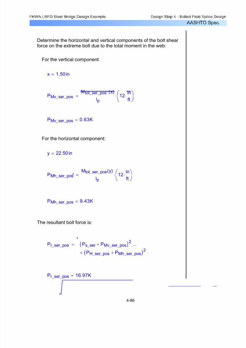
7/29/2019 LRFD steel design.pdf
http://slidepdf.com/reader/full/lrfd-steel-designpdf 285/646
Determine the horizontal and vertical components of the bolt shear force on the extreme bolt due to the total moment in the web:
For the vertical component:
x 1.50in=
PMv_ser_posMtot_ser_pos x( )⋅
Ip12
in
ft⋅⎛
⎝ ⎞ ⎠
⋅=
PMv_ser_pos 0.63K=
For the horizontal component:
y 22.50 in=
PMh_ser_posMtot_ser_pos y( )
Ip12
in
ft⋅⎛
⎝ ⎞ ⎠
⋅=
PMh_ser_pos 9.43K=
The resultant bolt force is:
Pr_ser_pos Ps_ser PMv_ser_pos+( )2
PH_ser_pos PMh_ser_pos+( )2+...=
Pr_ser_pos 16.97K=
4-86
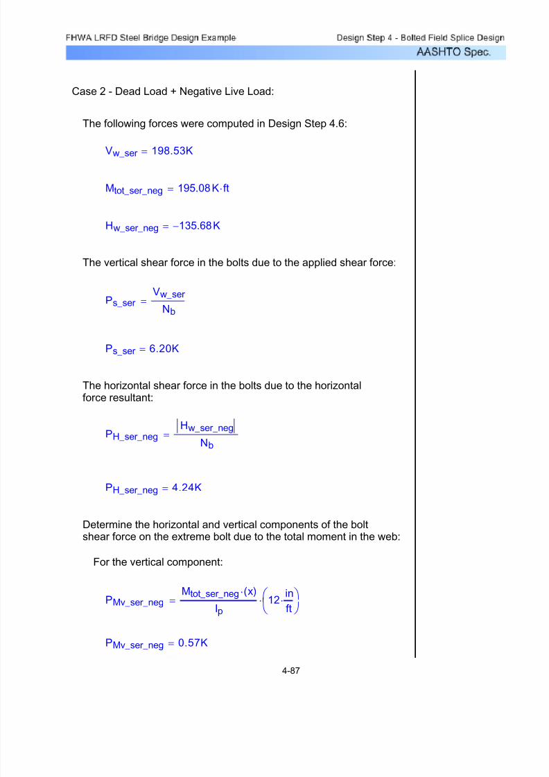
7/29/2019 LRFD steel design.pdf
http://slidepdf.com/reader/full/lrfd-steel-designpdf 286/646
Case 2 - Dead Load + Negative Live Load:
The following forces were computed in Design Step 4.6:
Vw_ser 198.53K=
Mtot_ser_neg 195.08K ft⋅=
Hw_ser_neg 135.68− K=
The vertical shear force in the bolts due to the applied shear force:
Ps_ser Vw_ser
Nb=
Ps_ser 6.20K=
The horizontal shear force in the bolts due to the horizontalforce resultant:
PH_ser_negHw_ser_neg
Nb=
PH_ser_neg 4.24K=
Determine the horizontal and vertical components of the boltshear force on the extreme bolt due to the total moment in the web:
For the vertical component:
PMv_ser_negMtot_ser_neg x( )⋅
Ip12
in
ft⋅⎛
⎝ ⎞ ⎠
⋅=
PMv_ser_neg 0.57K=
4-87

7/29/2019 LRFD steel design.pdf
http://slidepdf.com/reader/full/lrfd-steel-designpdf 287/646
For the horizontal component:
PMh_ser_neg
Mtot_ser_neg y( )
Ip12
in
ft⋅⎛ ⎝ ⎞ ⎠⋅=
PMh_ser_neg 8.51K=
The resultant bolt force is:
Pr_ser_neg Ps_ser PMv_ser_neg+( )2
PH_ser_neg PMh_ser_neg+( )2+
...=
Pr_ser_neg 14.43K=
The governing resultant bolt force is:
Pr_ser max Pr_ser_pos Pr_ser_neg,( )=
Pr_ser 16.97K=
Check:
Pr_ser
16.97K= < Rr
39.00K= OK
Thirty-two 7/8" diameter high-strength bolts in two verticalrows on each side of the splice provides sufficient resistanceagainst bolt shear and slip.
4-88

7/29/2019 LRFD steel design.pdf
http://slidepdf.com/reader/full/lrfd-steel-designpdf 288/646
OKRr 870.00K=<Vuw 279.05K=
Check:
Rr 870.00K=
Rr φv 0.58( )⋅ Agross_wp( )⋅ Fy( )⋅=
The factored shear resistance is then:
φv 1.0=Resistance factor for shear:
Fy 50ksi=Specified minimum yield strength of the connection element:
From Design Step 4.1:
Agross_wp 30.00in2
=
Agross_wp Nwp twp⋅ dwp⋅=
dwp 48 in⋅=Depth of splice plate:
twp 0.3125 in⋅=Thickness of plate:
Nwp 2=Number of splice plates:
The gross area of the web splice is calculated as follows:
SEquation
6.13.5.3-2
Rn 0.58 Ag⋅ Fy⋅=
SEquation
6.13.5.3-1Rr φv Rn⋅=
The factored resistance of the splice plates is taken as:
Vuw 279.05K=
Check for shear yielding on the gross section of the websplice plates under the Strength I design shear force, Vuw:
S6.13.6.1.4bShear Yielding of Splice Plates:
4-89

7/29/2019 LRFD steel design.pdf
http://slidepdf.com/reader/full/lrfd-steel-designpdf 289/646
Avn Nwp dwp Nfn dhole⋅−( )⋅ twp⋅= Nfn
where the net area resisting shear:
(Design Step 4.1)φbs 0.80=
SEquation 6.13.4-2Rr φbs 0.58 Fu⋅ Avn⋅ Fy Atg⋅+( )⋅=
Therefore, the factored resistance is:
Atn 0.0 in
2
⋅= Atg 0.0 in
2
⋅=
For this case, the areas of the plate resisting tension areconsidered to be zero.
Investigation of critical sections and failure modes, other thanblock shear, is recommended, including the case of a net sectionextending across the full plate width, and, therefore, having noparallel planes. This may be a more severe requirement for agirder flange or splice plate than the block shear rupture mode.
C6.13.4Fracture on the Net Section:
Vuw 279.05K=
From Design Step 4.6, the factored design shear for the Strength ILimit State was determined to be:
Strength I Limit State checks for fracture on the net section of websplice plates and block shear rupture normally do not govern for plates of typical proportion. These checks are provided in thisexample for completeness.
S6.13.6.1.4bFracture and Block Shear Rupture of the Web Splice Plates:
4-90

7/29/2019 LRFD steel design.pdf
http://slidepdf.com/reader/full/lrfd-steel-designpdf 290/646
OKVuw 279.05K=>Rr 603.20K=
Rr φbs 0.58 Fu⋅ Avn⋅( )⋅=
The factored resistance is then:
OK Avn 20.00in2
=> A85 25.50in2
=
Agross_wp 30.00in2
=
A85 0.85 Agross_wp⋅=
S6.13.5.2 Avn of the splice plates to be used in calculating the fracturestrength of the splice plates cannot exceed eighty-five percent of the gross area of the plates:
Avn 20.00in2=
Avn Nwp dwp Nfn dhole⋅−( )⋅ twp⋅=
Number of web plates: Nwp 2=
Depth of the web plate: dwp 48in=
Number of bolts along oneplane:
Nfn 16=
Thickness of the web plate: twp 0.3125in=
From Design Step 4.1:
Specified minimum yield strength of theconnected material:
Fy 50ksi=
Specified minimum tensile strength of theconnected material: Fu 65 ksi⋅=
Diameter of the bolt holes: dhole 1.0in=
Net area resisting shear:
4-91
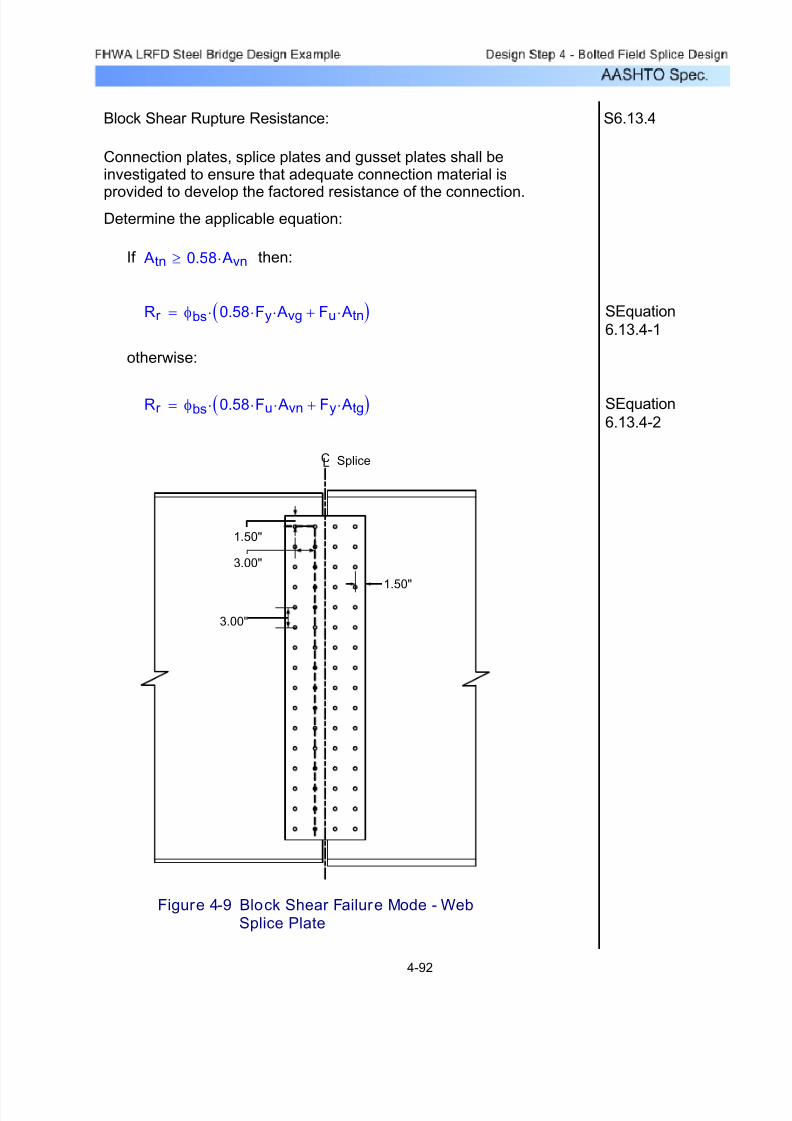
7/29/2019 LRFD steel design.pdf
http://slidepdf.com/reader/full/lrfd-steel-designpdf 291/646
Block Shear Rupture Resistance: S6.13.4
Connection plates, splice plates and gusset plates shall beinvestigated to ensure that adequate connection material is
provided to develop the factored resistance of the connection.Determine the applicable equation:
If Atn 0.58 Avn⋅≥ then:
Rr φbs 0.58 Fy⋅ Avg⋅ Fu Atn⋅+( )⋅= SEquation
6.13.4-1
otherwise:
Rr φbs 0.58 Fu⋅ Avn⋅ Fy Atg⋅+( )⋅= SEquation
6.13.4-2
3.00"
3.00"
1.50"
CL Splice
1.50"
Figure 4-9 Block Shear Failure Mode - WebSplice Plate
4-92
7/29/2019 LRFD steel design.pdf
http://slidepdf.com/reader/full/lrfd-steel-designpdf 292/646
OKRr 696.85K=<Vuw 279.05K=
Check:
Rr 696.85K=
Rr φbs 0.58 Fu⋅ Avn⋅ Fy Atg⋅+( )⋅=
Therefore, SEquation 6.13.4-2 is the governing equation:
0.58 Avn⋅ 11.24in2
=< Atn 1.88in2
=
Identify the appropriate block shear equation:
Atn 1.88in2=
Atn Nwp 1.50 in⋅ 3.0 in⋅+ 1.5 dhole( )⋅−⋅ twp⋅=
Net area along the plane resisting tension stress:
Atg 2.81in2
=
Atg Nwp 1.50 in⋅ 3.0 in⋅+( )⋅ twp⋅=
Gross area along the plane resisting tension stress:
Avn 19.38in2=
Avn Nwp dwp 1.50 in⋅− 15.50 dhole( )⋅−⋅ twp⋅=
Net area along the plane resisting shear stress:
Avg 29.06in2=
Avg Nwp dwp 1.50 in⋅−( )⋅ twp⋅=
Gross area along the plane resisting shear stress:
4-93

7/29/2019 LRFD steel design.pdf
http://slidepdf.com/reader/full/lrfd-steel-designpdf 293/646
OKφf Fy⋅ 50ksi=<f str_pos 39.94ksi=
f str_pos 39.94ksi=
f str_posMtot_str_pos
Spl
12in
ft⋅⎛
⎝
⎞
⎠
⋅Hw_str_pos
Agross_wp
+=
Hw_str_pos 486.20K=
Mtot_str_pos 474.66K ft⋅=
Case 1 - Dead Load + Positive Live Load:
Spl 240.00in3=
Spl1
6 Agross_wp⋅ dwp⋅=
Section modulus of the web splice plate:
φf 1.0=Resistance factor for flexure (Design Step 4.1):
where:
f MTotal
Spl
Huw
Agross_wp+ φf Fy⋅≤=
Huw
Check for flexural yielding on the gross section of the web spliceplates for the Strength I Limit State due to the total web momentand the horizontal force resultant:
S6.13.6.1.4bFlexural Yielding of Splice Plates:
4-94
7/29/2019 LRFD steel design.pdf
http://slidepdf.com/reader/full/lrfd-steel-designpdf 294/646
Case 2 - Dead Load + Negative Live Load:
Mtot_str_neg 734.19K ft⋅=
Hw_str_neg 140.16− K=
f str_negMtot_str_neg
Spl12
in
ft⋅⎛
⎝ ⎞ ⎠
⋅Hw_str_neg
Agross_wp+=
f str_neg 41.38ksi=
f str_neg 41.38ksi= < φf Fy⋅ 50ksi= OK
4-95
7/29/2019 LRFD steel design.pdf
http://slidepdf.com/reader/full/lrfd-steel-designpdf 295/646
OK0.95 Fy⋅ 47.50ksi=<f ser_pos 17.32ksi=
f ser_pos 17.32ksi=
f ser_posMtot_ser_pos
Spl12
in
ft⋅⎛
⎝ ⎞ ⎠
⋅Hw_ser_pos
Agross_wp+=
Hw_ser_pos 195.08K=
Mtot_ser_pos 216.34K ft⋅=
Case 1 - Dead Load + Positive Live Load:
Agross_wp 30.00in2
=
Spl 240.00in3
=
where:
f MTotal
Spl
Hw
Agross_wp+ 0.95 Fy⋅≤=
Hw
Check the maximum normal stress on the gross section of theweb splice plates for the Service II Limit State due to the total
web moment and horizontal force resultant:
S6.10.5.2Control of Permanent Deflection - Splice Plates:
4-96
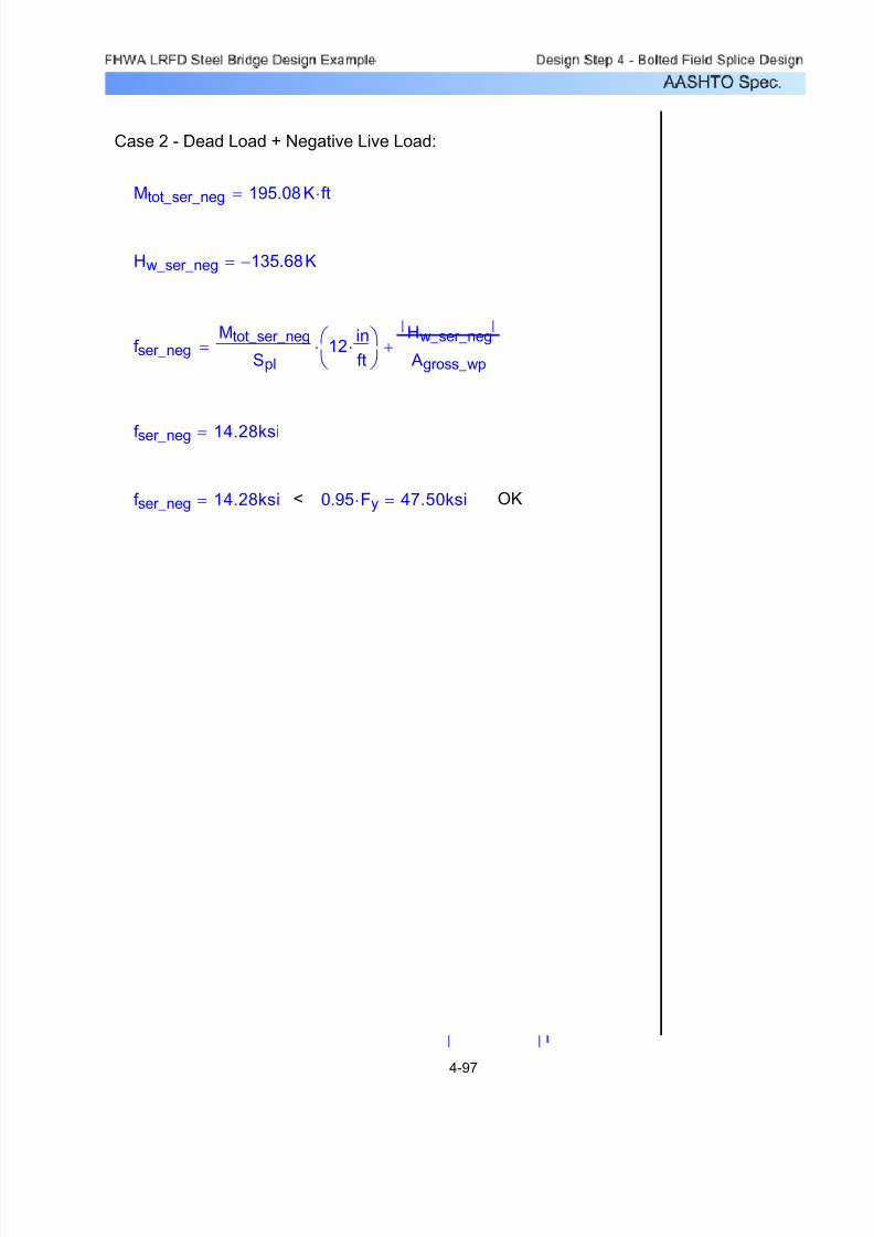
7/29/2019 LRFD steel design.pdf
http://slidepdf.com/reader/full/lrfd-steel-designpdf 296/646
Case 2 - Dead Load + Negative Live Load:
Mtot_ser_neg 195.08K ft⋅=
Hw_ser_neg 135.68− K=
f ser_negMtot_ser_neg
Spl12
in
ft⋅⎛
⎝ ⎞ ⎠
⋅Hw_ser_neg
Agross_wp+=
f ser_neg 14.28ksi=
f ser_neg 14.28ksi= < 0.95 Fy⋅ 47.50ksi= OK
4-97

7/29/2019 LRFD steel design.pdf
http://slidepdf.com/reader/full/lrfd-steel-designpdf 297/646
Web Bolts - Bearing Resistance at Bolt Holes: S6.13.2.9
Since the girder web thickness is less than twice the thickness of the web splice plates, the girder web will control for the bearingcheck.
Check the bearing of the bolts on the connected material for theStrength I Limit State assuming the bolts have slipped and gone intobearing. The design bearing strength of the girder web at thelocation of the extreme bolt in the splice is computed as the minimumresistance along the two orthogonal shear failure planes shown inFigure 4-10. The maximum force (vector resultant) acting on theextreme bolt is compared to this calculated strength, which isconservative since the components of this force parallel to the failuresurfaces are smaller than the maximum force.
Lc2
Hole 1
Hole 2
Lc1
Bottom Flange
End of
Girder
Shear Planes
for Bearing
(Typ.)
Figure 4-10 Bearing Resistance - Girder Web
To determine the applicable equation for the calculation of thenominal bearing resistance, the clear distance between holes and
the clear end distance must be calculated and compared to thevalue of two times the nominal diameter of the bolt. This checkyields:
S6.13.2.9
dbolt 0.875in= (Design Step 4.1)
2 dbolt⋅ 1.75in=
4-98
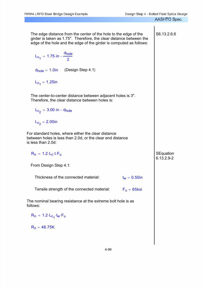
7/29/2019 LRFD steel design.pdf
http://slidepdf.com/reader/full/lrfd-steel-designpdf 298/646
Rn 48.75K=
Rn 1.2 Lc1
⋅ tw⋅ Fu⋅=
The nominal bearing resistance at the extreme bolt hole is asfollows:
Fu 65ksi=Tensile strength of the connected material:
tw 0.50in=Thickness of the connected material:
From Design Step 4.1:
SEquation6.13.2.9-2
Rn 1.2 Lc⋅ t⋅ Fu⋅=
For standard holes, where either the clear distancebetween holes is less than 2.0d, or the clear end distanceis less than 2.0d:
Lc22.00in=
Lc23.00 in⋅ dhole−=
The center-to-center distance between adjacent holes is 3".
Therefore, the clear distance between holes is:
Lc11.25in=
(Design Step 4.1)dhole 1.0in=
Lc11.75 in⋅
dhole
2−=
S6.13.2.6.6The edge distance from the center of the hole to the edge of thegirder is taken as 1.75". Therefore, the clear distance between theedge of the hole and the edge of the girder is computed as follows:
4-99

7/29/2019 LRFD steel design.pdf
http://slidepdf.com/reader/full/lrfd-steel-designpdf 299/646
The factored bearing resistance is:
Rr φbb Rn⋅=
φbb 0.80= (Design Step 4.1)
Rr 39.00K=
The controlling minimum Strength I resultant bolt force waspreviously computed:
Pr_str 37.98K= < Rr 39.00K= OK
Bearing Resistance at Web Bolt Holes
Should the bearing resistance be exceeded, it is
recommended that the edge distance be increasedslightly in lieu of increasing the number of bolts or thickening the web.
4-100
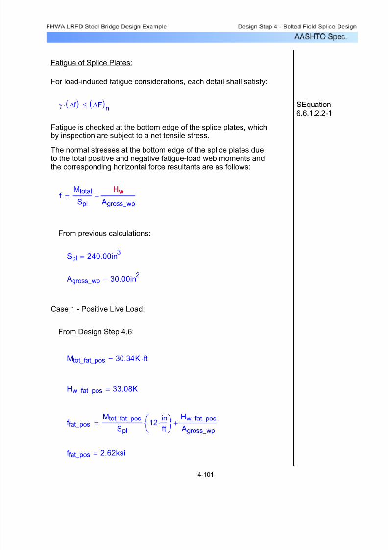
7/29/2019 LRFD steel design.pdf
http://slidepdf.com/reader/full/lrfd-steel-designpdf 300/646
f fat_pos 2.62ksi=
f fat_posMtot_fat_pos
Spl12
in
ft⋅⎛
⎝ ⎞ ⎠
⋅Hw_fat_pos
Agross_wp+=
Hw_fat_pos 33.08K=
Mtot_fat_pos 30.34K ft⋅=
From Design Step 4.6:
Case 1 - Positive Live Load:
Agross_wp 30.00in2=
Spl 240.00in3
=
From previous calculations:
f MtotalSpl
Hw Agross_wp
+= Hw
The normal stresses at the bottom edge of the splice plates dueto the total positive and negative fatigue-load web moments andthe corresponding horizontal force resultants are as follows:
Fatigue is checked at the bottom edge of the splice plates, whichby inspection are subject to a net tensile stress.
SEquation
6.6.1.2.2-1γ ∆f ( )⋅ ∆F( )
n≤
For load-induced fatigue considerations, each detail shall satisfy:
Fatigue of Splice Plates:
4-101
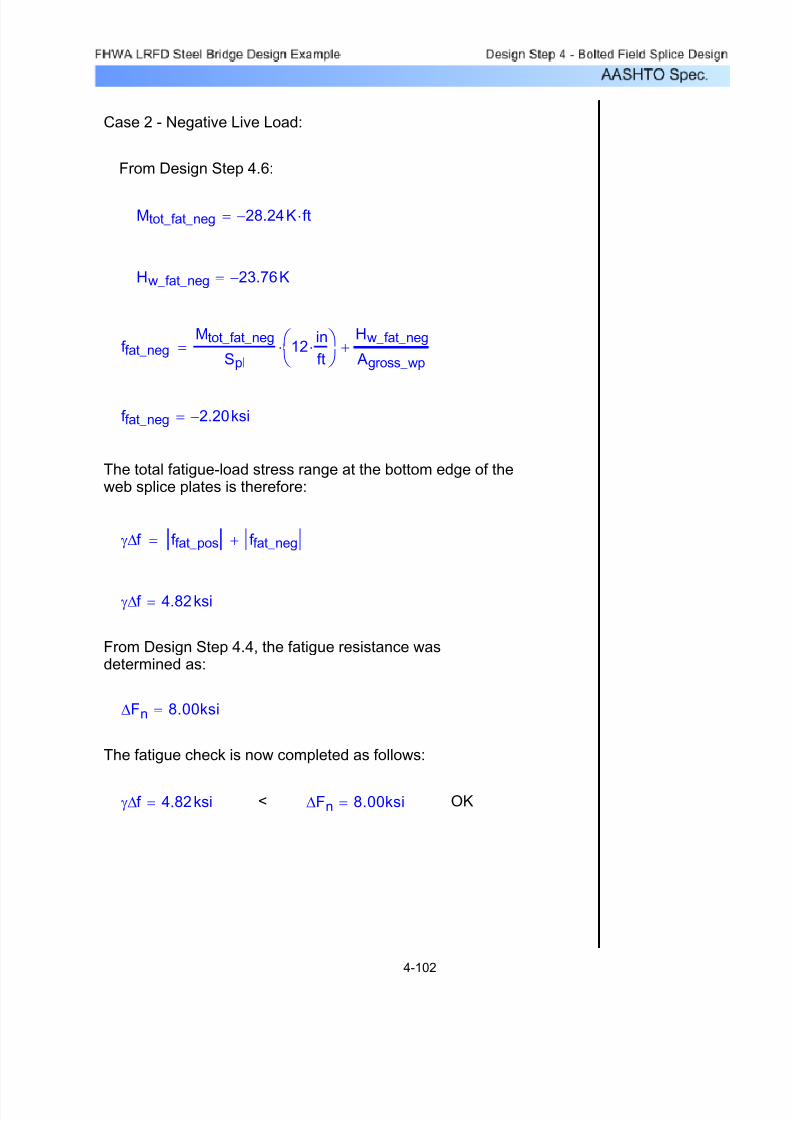
7/29/2019 LRFD steel design.pdf
http://slidepdf.com/reader/full/lrfd-steel-designpdf 301/646
OK∆Fn 8.00ksi=<γ∆f 4.82ksi=
The fatigue check is now completed as follows:
∆Fn 8.00ksi=
From Design Step 4.4, the fatigue resistance wasdetermined as:
γ∆f 4.82ksi=
γ∆f f fat_pos f fat_neg+=
The total fatigue-load stress range at the bottom edge of theweb splice plates is therefore:
f fat_neg 2.20− ksi=
f fat_negMtot_fat_neg
Spl12
in
ft⋅⎛
⎝ ⎞ ⎠
⋅Hw_fat_neg
Agross_wp+=
Hw_fat_neg 23.76− K=
Mtot_fat_neg 28.24− K ft⋅=
From Design Step 4.6:
Case 2 - Negative Live Load:
4-102
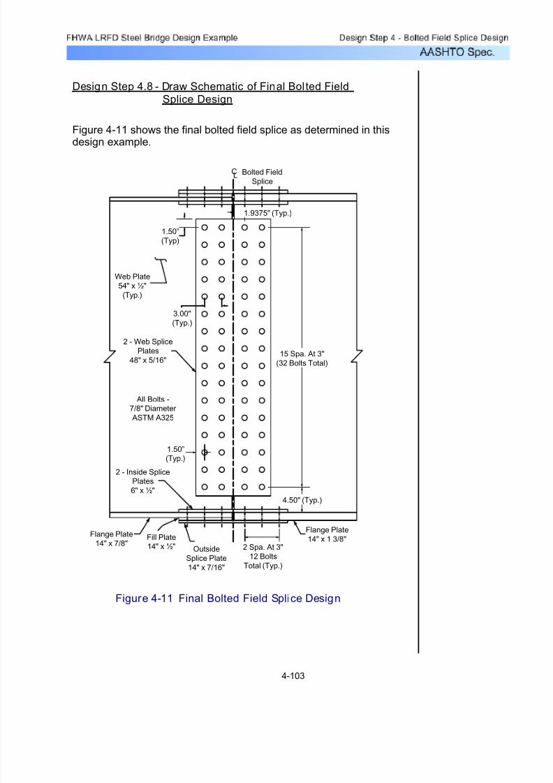
7/29/2019 LRFD steel design.pdf
http://slidepdf.com/reader/full/lrfd-steel-designpdf 302/646
Design Step 4.8 - Draw Schematic of Final Bolted Field
Splice Design
Figure 4-11 shows the final bolted field splice as determined in thisdesign example.
2 - Web Splice
Plates
48" x 5/16"
1.50”
(Typ)
3.00"
(Typ.)
1.9375" (Typ.)
Fill Plate
14" x ½" OutsideSplice Plate
14" x 7/16"
Flange Plate
14" x 7/8"
Flange Plate
14" x 1 3/8"
2 - Inside Splice
Plates
6" x ½"
15 Spa. At 3"
(32 Bolts Total)
4.50" (Typ.)
All Bolts -
7/8" Diameter ASTM A325
2 Spa. At 3"12 Bolts
Total (Typ.)
1.50”
(Typ.)
Web Plate54" x ½"
(Typ.)
C Bolted Field
SpliceL
Figure 4-11 Final Bolted Field Splice Design
4-103

7/29/2019 LRFD steel design.pdf
http://slidepdf.com/reader/full/lrfd-steel-designpdf 303/646
Refer to Design Step 1 for introductory information about this designexample. Additional information is presented about the designassumptions, methodology, and criteria for the entire bridge, includingthe design features included in this design step.
ksf K
ft2=ksi
K
in2=K 1000lb=
Design Step 5 consists of various design computations associatedwith the steel girder but not necessarily required to design the actualplates of the steel girder. Such miscellaneous steel designcomputations include the following:
1. Shear connectors2. Bearing stiffeners3. Welded connections
4. Diaphragms and cross-frames5. Lateral bracing6. Girder camber
For this design example, computations for the shear connectors, abearing stiffener, a welded connection, and a cross-frame will bepresented. The other features must also be designed, but their design computations are not included in this design example.
The following units are defined for use in this design example:
(It should be noted that Design Step 5.4presents a narrative description rather thandesign computations.)
21Design Step 5.4 - Design Cross-frames
16Design Step 5.3 - Design Welded Connections
10Design Step 5.2 - Design Bearing Stiffeners
2Design Step 5.1 - Design Shear Connectors
PageTable of Contents
Miscellaneous Steel Design ExampleDesign Step 5
5-1

7/29/2019 LRFD steel design.pdf
http://slidepdf.com/reader/full/lrfd-steel-designpdf 304/646
Design Step 5.1 - Design Shear Connectors
Since the steel girder has been designed as a composite section,shear connectors must be provided at the interface between the
concrete deck slab and the steel section to resist the interface shear.For continuous composite bridges, shear connectors are normallyprovided throughout the length of the bridge. In the negative flexureregion, since the longitudinal reinforcement is considered to be a partof the composite section, shear connectors must be provided.
Studs or channels may be used as shear connectors. For this designexample, stud shear connectors are being used throughout the lengthof the bridge. The shear connectors must permit a thoroughcompaction of the concrete to ensure that their entire surfaces are incontact with the concrete. In addition, the shear connectors must be
capable of resisting both horizontal and vertical movement betweenthe concrete and the steel.
The following figure shows the stud shear connector proportions, aswell as the location of the stud head within the concrete deck.
S6.10.7.4.1
S6.10.7.4.1a
7/8"φ
14"
8 ½ "
5"
(Typ.)
A
B
C
6 "
3 ½ "
Figure 5-1 Stud Shear Connectors
Flexure Region A B C
Positive 2.875" 3.125" 5.375"
Intermediate 2.25" 3.75" 4.75"
Negative 1.00” 5.00” 3.50”
Shear Connector Embedment
Table 5-1 Shear Connector Embedment
5-2
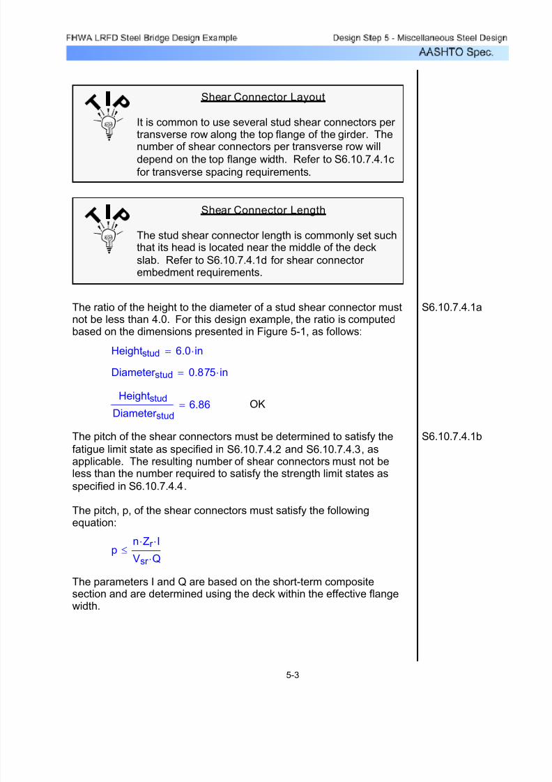
7/29/2019 LRFD steel design.pdf
http://slidepdf.com/reader/full/lrfd-steel-designpdf 305/646
The parameters I and Q are based on the short-term compositesection and are determined using the deck within the effective flangewidth.
pn Z
r ⋅ I⋅
Vsr Q⋅≤
S6.10.7.4.1bThe pitch of the shear connectors must be determined to satisfy the
fatigue limit state as specified in S6.10.7.4.2 and S6.10.7.4.3, asapplicable. The resulting number of shear connectors must not beless than the number required to satisfy the strength limit states as
specified in S6.10.7.4.4.
The pitch, p, of the shear connectors must satisfy the followingequation:
OKHeightstud
Diameter stud6.86=
Diameter stud 0.875 in⋅=
Heightstud 6.0 in⋅=
S6.10.7.4.1aThe ratio of the height to the diameter of a stud shear connector mustnot be less than 4.0. For this design example, the ratio is computedbased on the dimensions presented in Figure 5-1, as follows:
Shear Connector Length
The stud shear connector length is commonly set suchthat its head is located near the middle of the deck
slab. Refer to S6.10.7.4.1d for shear connector
embedment requirements.
Shear Connector Layout
It is common to use several stud shear connectors per
transverse row along the top flange of the girder. Thenumber of shear connectors per transverse row will
depend on the top flange width. Refer to S6.10.7.4.1c
for transverse spacing requirements.
5-3

7/29/2019 LRFD steel design.pdf
http://slidepdf.com/reader/full/lrfd-steel-designpdf 306/646
p 10.04 in=pn Zr ⋅ I⋅
Vsr Q⋅=
Zr 2.11 K⋅=Therefore,
5.5 d2⋅
22.11=α d
2⋅ 0.48=
ind 0.875=
α 0.626=
α 34.5 4.28 log N( )⋅−=
S6.6.1.2.5(see Design Step 3.14 at locationof maximum positive flexure)
N 82125000=
S6.10.7.4.2Zr α d2⋅
5.5 d2⋅
2≥= d
(see live load analysis computer run)
Vsr 34.97K=
Vsr 0.75 41.45 K⋅ 5.18 K⋅+( )⋅=
In the positive flexure region, the maximum fatigue live loadshear range is located at the abutment. The factored value iscomputed as follows:
Q 1195.8 in3=
Q8.0 in⋅( ) 103.0 in⋅( )⋅
8
⎡⎣
⎤⎦
62.375 in⋅ 50.765 in⋅−( )⋅=
S6.10.3.1.1b(see Table 3-4)I 66340.3 in4⋅=
(see Figure 5-1)n 3=
In the positive flexure region:
5-4

7/29/2019 LRFD steel design.pdf
http://slidepdf.com/reader/full/lrfd-steel-designpdf 307/646
p 10 in⋅=
Therefore, based on the above pitch computations to satisfy thefatigue limit state, use the following pitch throughout the entire girder length:
p 13.07 in=pn Zr ⋅ I⋅
Vsr Q⋅=
(see previous computation)Zr 2.11 K⋅=
S6.10.7.4.2Zr α d2⋅
5.5 d2⋅
2≥=
(see Table 3-1 and live load analysis computer run)
Vsr 34.90K=
Vsr 0.75 0.00 K⋅ 46.53 K⋅+( )⋅=
Q 1807.4 in3=
Q8.0 in⋅( ) 103.0 in⋅( )⋅
8
⎡
⎣
⎤
⎦
64.250 in⋅ 46.702 in⋅−( )⋅=
(see Table 3-5)I 130196.1 in4⋅=
SC6.10.7.4.1bIn the negative flexure region, the parameters I and Q may
be determined using the reinforcement within the effectiveflange width for negative moment, unless the concrete slabis considered to be fully effective for negative moment incomputing the longitudinal range of stress, as permitted in
S6.6.1.2.1. For this design example, I and Q are assumedto be computed considering the concrete slab to be fullyeffective.
(see Figure 5-1)n 3=
In the negative flexure region:
5-5
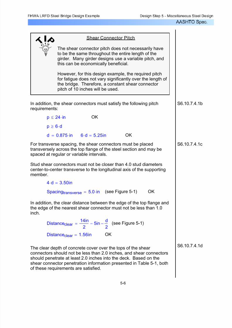
7/29/2019 LRFD steel design.pdf
http://slidepdf.com/reader/full/lrfd-steel-designpdf 308/646
The clear depth of concrete cover over the tops of the shear connectors should not be less than 2.0 inches, and shear connectorsshould penetrate at least 2.0 inches into the deck. Based on theshear connector penetration information presented in Table 5-1, bothof these requirements are satisfied.
S6.10.7.4.1d
OKDistanceclear 1.56in=
(see Figure 5-1)Distanceclear 14in
25in−
d
2−=
In addition, the clear distance between the edge of the top flange andthe edge of the nearest shear connector must not be less than 1.0inch.
OK(see Figure 5-1)Spacingtransverse 5.0 in⋅=
4 d⋅ 3.50in=
S6.10.7.4.1cFor transverse spacing, the shear connectors must be placedtransversely across the top flange of the steel section and may bespaced at regular or variable intervals.
Stud shear connectors must not be closer than 4.0 stud diameterscenter-to-center transverse to the longitudinal axis of the supportingmember.
OK6 d⋅ 5.25in=d 0.875 in⋅=
p 6 d⋅≥
OKp 24 in⋅≤
S6.10.7.4.1bIn addition, the shear connectors must satisfy the following pitchrequirements:
Shear Connector Pitch
The shear connector pitch does not necessarily haveto be the same throughout the entire length of the
girder. Many girder designs use a variable pitch, andthis can be economically beneficial.
However, for this design example, the required pitchfor fatigue does not vary significantly over the length of the bridge. Therefore, a constant shear connector pitch of 10 inches will be used.
5-6

7/29/2019 LRFD steel design.pdf
http://slidepdf.com/reader/full/lrfd-steel-designpdf 309/646
S6.4.4
0.5 0.601⋅ 4.0 3834⋅⋅ 37.21= K
0.601 60.0⋅ 36.06= K
Therefore, Qn 36.06 K⋅=
Qr φsc Qn⋅=
Therefore, Qr 30.65K=
The number of shear connectors provided between the section of maximum positive moment and each adjacent point of 0.0 momentor between each adjacent point of 0.0 moment and the centerline of an interior support must not be less than the following:
S6.10.7.4.4a
nVh
Qr =
Vh
The total horizontal shear force, Vh, between the point of maximum
positive moment and each adjacent point of 0.0 moment is equal tothe lesser of the following:
S6.10.7.4.4b
Vh 0.85 f'c⋅ b⋅ ts⋅= ts
or
Vh Fyw D⋅ tw⋅ Fyt bt⋅ tt⋅+ Fyc bf ⋅ tf ⋅+= tf
For the strength limit state, the factored resistance of the shear connectors, Qr , is computed as follows:
S6.10.7.4.4
Qr φsc Qn⋅= Qn S6.10.7.4.4a
φsc 0.85= S6.5.4.2
The nominal shear resistance of one stud shear connector embedded in a concrete slab is computed as follows:
S6.10.7.4.4c
Qn 0.5 Asc⋅ f'c Ec⋅⋅ Asc Fu⋅≤= Fu
Asc πd
2
4⋅= Asc 0.601in
2=
f'c 4.0 ksi⋅= (see Design Step 3.1) S5.4.2.1
Ec 3834 ksi⋅= (see Design Step 3.3) S5.4.2.4
Fu 60.0 ksi⋅=
5-7

7/29/2019 LRFD steel design.pdf
http://slidepdf.com/reader/full/lrfd-steel-designpdf 310/646
Fyc 50 ksi⋅= (see Design Step 3.1) STable 6.4.1-1
bf 14 in⋅= (see Design Step 3.18)
tf 0.625 in⋅= (see Design Step 3.18)
0.85 f'c⋅ b⋅ ts⋅ 2802K=
Fyw D⋅ tw⋅ Fyt bt⋅ tt⋅+ Fyc bf ⋅ tf ⋅+ 2400K=
Therefore, Vh 2400 K⋅=
Therefore, the number of shear connectors provided between thesection of maximum positive moment and each adjacent point of 0.0 moment must not be less than the following:
S6.10.7.4.4a
nVh
Qr =
n 78.3=
The distance between the end of the girder and the location of maximum positive moment is approximately equal to:
L 48.0 ft⋅= (see Table 3-7)
Similarly the distance between the section of the maximum positivemoment and the point of dead load contraflexure is approximatelyequal to:
L 83.6 ft⋅ 48.0 ft⋅−= (see Table 3-7)
L 35.6ft=
where f'c 4.0ksi= (see Design Step 3.1) S5.4.2.1
b 103.0 in⋅= (see Design Step 3.3)
ts 8.0 in⋅= (see Design Step 3.1)
Fyw 50 ksi⋅= (see Design Step 3.1) STable 6.4.1-1
D 54 in⋅= (see Design Step 3.18)
tw 0.50 in⋅= (see Design Step 3.18)
Fyt 50 ksi⋅= (see Design Step 3.1) STable 6.4.1-1
bt 14 in⋅= (see Design Step 3.18)
tt 0.875 in⋅= (see Design Step 3.18)
5-8
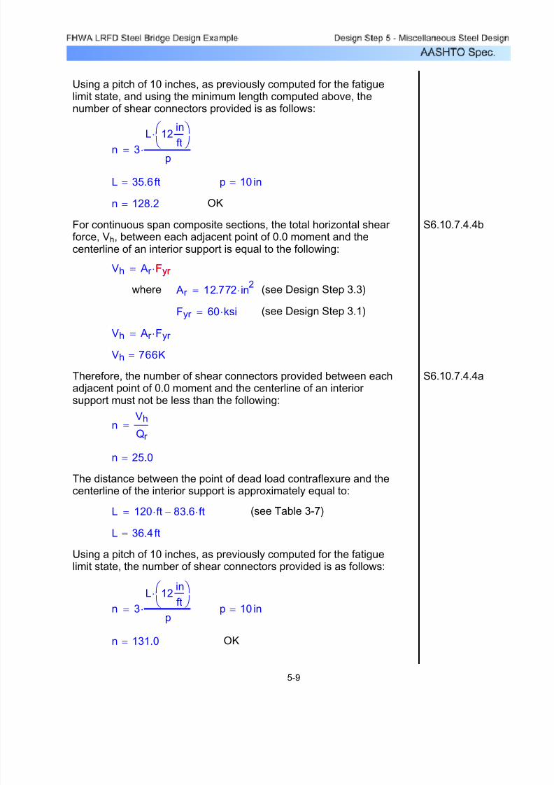
7/29/2019 LRFD steel design.pdf
http://slidepdf.com/reader/full/lrfd-steel-designpdf 311/646
OKn 131.0=
p 10 in=n 3
L 12in
ft
⎛ ⎝
⎞ ⎠
⋅
p⋅=
Using a pitch of 10 inches, as previously computed for the fatiguelimit state, the number of shear connectors provided is as follows:
L 36.4ft=
(see Table 3-7)L 120 ft⋅ 83.6 ft⋅−=
The distance between the point of dead load contraflexure and thecenterline of the interior support is approximately equal to:
n 25.0=
nVh
Qr =
S6.10.7.4.4aTherefore, the number of shear connectors provided between eachadjacent point of 0.0 moment and the centerline of an interior support must not be less than the following:
Vh 766K=
Vh Ar Fyr ⋅=
(see Design Step 3.1)Fyr 60 ksi⋅=
(see Design Step 3.3) Ar 12.772 in2⋅=where
Vh
Ar
Fyr
⋅= Fyr
S6.10.7.4.4bFor continuous span composite sections, the total horizontal shear force, Vh, between each adjacent point of 0.0 moment and thecenterline of an interior support is equal to the following:
OKn 128.2=
p 10 in=L 35.6ft=
n 3L 12
in
ft
⎛ ⎝
⎞ ⎠⋅
p⋅=
Using a pitch of 10 inches, as previously computed for the fatiguelimit state, and using the minimum length computed above, thenumber of shear connectors provided is as follows:
5-9

7/29/2019 LRFD steel design.pdf
http://slidepdf.com/reader/full/lrfd-steel-designpdf 312/646
Therefore, using a pitch of 10 inches for each row, with three studshear connectors per row, throughout the entire length of the girder
satisfies both the fatigue limit state requirements of S6.10.7.4.1 and
S6.10.7.4.2 and the strength limit state requirements of S6.10.7.4.4.
Therefore, use a shear stud spacing as illustrated in the followingfigure.
Symmetrical about L Pier
144 Spaces @ 10" = 120'-0"
(3 Stud Shear Connectors Per Row)
L Pier CL Bearing AbutmentC
C
Figure 5-2 Shear Connector Spacing
Design Step 5.2 - Design Bearing Sti ffeners
Bearing stiffeners are required to resist the bearing reactions andother concentrated loads, either in the final state or duringconstruction.
For plate girders, bearing stiffeners are required to be placed on thewebs at all bearing locations and at all locations supportingconcentrated loads.
Therefore, for this design example, bearing stiffeners are required atboth abutments and at the pier. The following design of the abutmentbearing stiffeners illustrates the bearing stiffener design procedure.
The bearing stiffeners in this design example consist of one platewelded to each side of the web. The connections to the web will bedesigned to transmit the full bearing force due to factored loads andis presented in Design Step 5.3.
S6.10.8.2.1
5-10
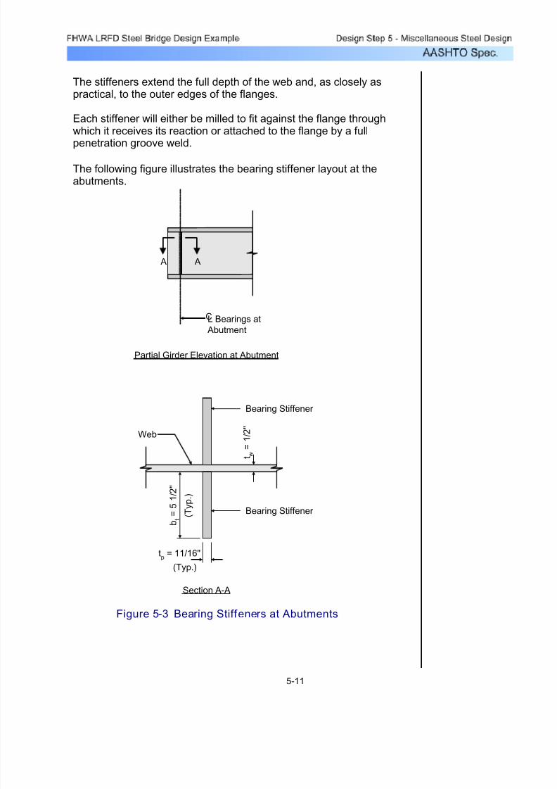
7/29/2019 LRFD steel design.pdf
http://slidepdf.com/reader/full/lrfd-steel-designpdf 313/646
The stiffeners extend the full depth of the web and, as closely aspractical, to the outer edges of the flanges.
Each stiffener will either be milled to fit against the flange throughwhich it receives its reaction or attached to the flange by a fullpenetration groove weld.
The following figure illustrates the bearing stiffener layout at theabutments.
L Bearings at
Abutment
A A
Partial Girder Elevation at Abutment
Section A-A
t w = 1 / 2 "
b t = 5 1 / 2 "
tp = 11/16"
Web
Bearing Stiffener
Bearing Stiffener
( T y p . )
(Typ.)
C
Figure 5-3 Bearing Stiffeners at Abutments
5-11

7/29/2019 LRFD steel design.pdf
http://slidepdf.com/reader/full/lrfd-steel-designpdf 314/646
Part of the stiffener must be clipped to clear theweb-to-flange weld. Thus the area of direct bearing isless than the gross area of the stiffener. The bearingarea, Apn, is taken as the area of the projecting elementsof the stiffener outside of the web-to-flange fillet welds butnot beyond the edge of the flange. This is illustrated inthe following figure:
S6.5.4.2 φb 1.00=
Br φb Apn⋅ Fys⋅= Apn
S6.10.8.2.3 The bearing resistance must be sufficient to resist the factoredreaction acting on the bearing stiffeners. The factored bearingresistance, Br , is computed as follows:
OK(see Figure 5-3)bt 5.5 in⋅=
0.48 tp⋅E
Fys⋅ 7.95in=
STable 6.4.1-1 Fys 50 ksi⋅=
S6.4.1 E 29000 ksi⋅=
(see Figure 5-3)tp11
16in⋅=
bt 0.48 tp⋅
E
Fys⋅≤
S6.10.8.2.2 The projecting width, bt, of each bearing stiffener element mustsatisfy the following equation. This provision is intended to preventlocal buckling of the bearing stiffener plates.
Bearing Stiffener Plates
Bearing stiffeners usually consist of one plateconnected to each side of the web. This is generally agood starting assumption for the bearing stiffener design. Then, if this configuration does not providesufficient resistance, two plates can be used on eachside of the web.
5-12

7/29/2019 LRFD steel design.pdf
http://slidepdf.com/reader/full/lrfd-steel-designpdf 315/646
1"
Bearing
Stiffener
(Typ.)
1" x 1" Clip for
Fillet Weld (Typ.)
Total Width = 5 1/2"
Bearing Width = 4 1/2"
Figure 5-4 Bearing Width
bbrg bt 1.0 in⋅−= bbrg 4.5in=
Apn 2bbrg tp⋅= Apn 6.19in2=
Fys 50ksi=
Br φb Apn⋅ Fys⋅=
Br 309.4K=
The factored bearing reaction at the abutment is computed as
follows, using load factors as presented in STable 3.4.1-1 and
STable 3.4.1-2 and using reactions obtained from a computer analysis run:
ReactionFactored 1.25 68.7⋅ K⋅( ) 1.50 11.0⋅ K⋅( )+1.75 110.5⋅ K⋅( )+
...=
ReactionFactored 295.8K=
Therefore, the bearing stiffener at the abutment satisfies the bearingresistance requirements.
5-13

7/29/2019 LRFD steel design.pdf
http://slidepdf.com/reader/full/lrfd-steel-designpdf 316/646
Is 87.22in4=
Is0.6875in 11.5in( )
3⋅ 8.3125in 0.5in( )3⋅+
12= S6.10.8.2.4b
S6.10.8.2.4akl 0.75( ) 54in( )⋅=
S6.9.4.1λk l⋅
r s π⋅⎛ ⎝
⎞ ⎠
2 Fy
E⋅=Fy
S6.5.4.2φc 0.90=
S6.9.2.1Pr φc Pn⋅= Pn
Figure 5-5 Bearing Stiffener Effect ive Section
t w = 1 / 2 "
b t = 5 1 / 2 "
tp
= 11/16"
Bearing Stiffener
(Typ.)
( T y p . )
(Typ.)
9tw
= 4 1/2" 9tw
= 4 1/2"
9"
Midthickness
of Web
S6.10.8.2.4b
S6.10.8.2.4a
S6.10.8.2.4 The final bearing stiffener check relates to the axial resistance of thebearing stiffeners. The factored axial resistance is determined as
specified in S6.9.2.1. The radius of gyration is computed about themidthickness of the web, and the effective length is taken as 0.75D,
where D is the web depth.
For stiffeners consisting of two plates welded to the web, the effectivecolumn section consists of the two stiffener elements, plus a centrallylocated strip of web extending not more than 9tw on each side of thestiffeners. This is illustrated in the following figure:
5-14

7/29/2019 LRFD steel design.pdf
http://slidepdf.com/reader/full/lrfd-steel-designpdf 317/646
Therefore, the bearing stiffener at the abutment satisfies the axialbearing resistance requirements.
The bearing stiffener at the abutment satisfies all bearing stiffener requirements. Therefore, use the bearing stiffener as presented inFigures 5-3 and 5-4.
ReactionFactored 295.8K=
Pr 533.9K=
S6.9.2.1Pr φc Pn⋅=
Pn 593.3K=
S6.9.4.1Pn 0.66λ
Fy As⋅=Therefore,
λ 2.25≤Therefore,
λ 0.0396=
S6.9.4.1λkl
r s π⋅⎛ ⎝
⎞ ⎠
2 Fy
E⋅=
Fy 50ksi=
r s 2.69in=
r sIs
As=
As 12.06in2=
S6.10.8.2.4b As 0.6875in 11.5⋅ in( ) 8.3125in 0.5⋅ in( )+=
5-15
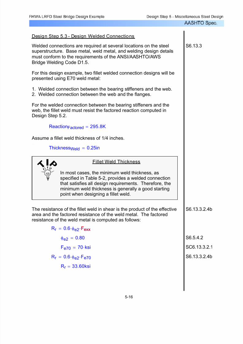
7/29/2019 LRFD steel design.pdf
http://slidepdf.com/reader/full/lrfd-steel-designpdf 318/646
Rr 33.60ksi=
S6.13.3.2.4bRr 0.6 φe2⋅ Fe70⋅=
SC6.13.3.2.1Fe70 70 ksi⋅=
S6.5.4.2φe2
0.80=
Rr 0.6 φe2⋅ Fexx⋅= Fexx
S6.13.3.2.4bThe resistance of the fillet weld in shear is the product of the effectivearea and the factored resistance of the weld metal. The factoredresistance of the weld metal is computed as follows:
Fillet Weld Thickness
In most cases, the minimum weld thickness, asspecified in Table 5-2, provides a welded connectionthat satisfies all design requirements. Therefore, theminimum weld thickness is generally a good startingpoint when designing a fillet weld.
ThicknessWeld 0.25in=
Assume a fillet weld thickness of 1/4 inches.
ReactionFactored 295.8K=
S6.13.3 Welded connections are required at several locations on the steelsuperstructure. Base metal, weld metal, and welding design details
must conform to the requirements of the ANSI/AASHTO/AWS
Bridge Welding Code D1.5.
For this design example, two fillet welded connection designs will bepresented using E70 weld metal:
1. Welded connection between the bearing stiffeners and the web.2. Welded connection between the web and the flanges.
For the welded connection between the bearing stiffeners and theweb, the fillet weld must resist the factored reaction computed inDesign Step 5.2.
Design Step 5.3 - Design Welded Connections
5-16

7/29/2019 LRFD steel design.pdf
http://slidepdf.com/reader/full/lrfd-steel-designpdf 319/646
In this case, the thicker part joined is the bearing stiffener plate,which is 11/16 inches thick. Therefore, based on Table 5-2, theminimum size of fillet weld is 1/4 inch, and this requirement issatisfied.
Table 5-2 Minimum Size of Fillet Welds
STable 6.13.3.4-1Base Metal Thickness of
Thicker Part Joined (T)
(Inches)
Minimum Size of
Fillet Weld
(Inches)
T ≤ 3/4 1/4
T>
3/4 5/16
Minimum Size of Fillet Welds
S6.13.3.4
S6.13.3.4For material 0.25 inches or more in thickness, the maximum size of the fillet weld is 0.0625 inches less than the thickness of the material,unless the weld is designated on the contract documents to be builtout to obtain full throat thickness.
For the fillet weld connecting the bearing stiffeners to the web, thebearing stiffener thickness is 11/16 inches and the web thickness is1/2 inches. Therefore, the maximum fillet weld size requirement issatisfied.
The minimum size of fillet welds is as presented in Table 5-2. Inaddition, the weld size need not exceed the thickness of the thinner part joined.
OKResistance 1235K=
Resistance Rr AreaEff ⋅=
S6.13.3.2.4bThe resistance of the fillet weld is then computed as follows:
AreaEff 36.77in2= AreaEff LengthEff ThroatEff ⋅=
ThroatEff 0.177in=ThroatEff ThicknessWeld
2=
LengthEff 208.0in=LengthEff 4 54in 2in−( )⋅=
S6.13.3.3The effective area equals the effective weld length multiplied by theeffective throat. The effective throat is the shortest distance from the
joint root to the weld face.
5-17
7/29/2019 LRFD steel design.pdf
http://slidepdf.com/reader/full/lrfd-steel-designpdf 320/646
The minimum effective length of a fillet weld is four times its size andin no case less than 1.5 inches. Therefore, this requirement is alsosatisfied.
Since all weld design requirements are satisfied, use a 1/4 inch filletweld for the connection of the bearing stiffeners to the web.
S6.13.3.5
For the welded connection between the web and the flanges, the filletweld must resist a factored horizontal shear per unit length based onthe following equation:
S6.13.3
vV Q⋅
I=
V
This value is greatest at the pier, where the factored shear has its
highest value.
The following computations are for the welded connection betweenthe web and the top flange. The welded connection between the weband the bottom flange is designed in a similar manner.
The shear is computed based on the individual section propertiesand load factors for each loading, as presented in Design Steps 3.3and 3.6:
For the noncomposite section, the factored horizontal shear is
computed as follows:
VNoncomp 1.25 114.7⋅ K⋅( )=
VNoncomp 143.4K=
QNoncomp 14 in⋅ 2.5⋅ in⋅( ) 58.00 in⋅ 28.718 in⋅−( )⋅=
QNoncomp 1024.9in3=
INoncomp 65426.6 in4⋅=
vNoncompVNoncomp QNoncomp⋅
INoncomp= vNoncomp 2.25
K
in=
5-18

7/29/2019 LRFD steel design.pdf
http://slidepdf.com/reader/full/lrfd-steel-designpdf 321/646
AreaEff 0.442in
2
in= AreaEff 2 ThroatEff ⋅=
ThroatEff 0.221in=ThroatEff ThicknessWeld
2=
S6.13.3.3The effective area equals the effective weld length multiplied by theeffective throat. The effective throat is the shortest distance from the
joint root to the weld face. In this case, the effective area is computed
per unit length, based on the use of one weld on each side of the web.
Rr 33.60ksi=Rr 0.6 φe2⋅ Fe70⋅=
S6.13.3.2.4bThe resistance of the fillet weld in shear is the product of the effectivearea and the factored resistance of the weld metal. The factoredresistance of the weld metal was previously computed as follows:
ThicknessWeld 0.3125in=
Assume a fillet weld thickness of 5/16 inches.
vTotal 5.38K
in=
vTotal vNoncomp vComp+=
Based on the above computations, the total factored horizontalshear is computed as follows:
vComp 3.13K
in=vComp
VComp QComp⋅
IComp
=
IComp 79333.4 in4⋅=
QComp 886.6in3=
QComp 14 in⋅ 2.5⋅ in⋅( ) 58.00 in⋅ 32.668 in⋅−( )⋅=
VComp 280.1K=
VComp 1.25 16.4⋅ K⋅( ) 1.50 19.8⋅ K⋅( )+ 1.75 131.4⋅ K⋅( )+=
For the composite section, the factored horizontal shear iscomputed as follows:
5-19
7/29/2019 LRFD steel design.pdf
http://slidepdf.com/reader/full/lrfd-steel-designpdf 322/646
The resistance of the fillet weld is then computed as follows: S6.13.3.2.4b
Resistance Rr AreaEff ⋅=
Resistance 14.85
K
in=OK
For material 0.25 inches or more in thickness, the maximum size of the fillet weld is 0.0625 inches less than the thickness of the material,unless the weld is designated on the contract documents to be builtout to obtain full throat thickness.
For the fillet weld connecting the web to the flanges, the webthickness is 0.5 inches, the minimum flange thickness is 0.625inches, and the maximum flange thickness is 2.75 inches. Therefore,the maximum fillet weld size requirement is satisfied.
The minimum size of fillet welds is as presented in Table 5-2. Inaddition, the weld size need not exceed the thickness of the thinner part joined.
S6.13.3.4
S6.13.3.4
In this case, the thicker part joined is the flange, which has a minimumthickness of 0.625 inches and a maximum thickness of 2.75 inches.Therefore, based on Table 5-2, the minimum size of fillet weld is 5/16inch, and this requirement is satisfied.
The minimum effective length of a fillet weld is four times its size andin no case less than 1.5 inches. Therefore, this requirement is also
satisfied.
Since all weld design requirements are satisfied, use a 5/16 inch filletweld for the connection of the web and the top flange. The weldedconnection between the web and the bottom flange is designed in asimilar manner.
S6.13.3.5
Load-induced fatigue must be considered in the base metal at a weldedconnection. Fatigue considerations for plate girders may include:
1. Welds connecting the shear studs to the girder.
2. Welds connecting the flanges and the web.3. Welds connecting the transverse intermediate stiffeners to the girder.
The specific fatigue considerations depend on the unique characteristicsof the girder design. Specific fatigue details and detail categories are
explained and illustrated in STable 6.6.1.2.3-1 and in SFigure
6.6.1.2.3-1.
S6.6.1.2.5
5-20

7/29/2019 LRFD steel design.pdf
http://slidepdf.com/reader/full/lrfd-steel-designpdf 323/646
In Design Step 3.14 for the positive moment region, the fatigue check isillustrated for the fillet-welded connection of the transverse intermediatestiffeners to the girder. This procedure must be considered for thebase metal at welded connections.
Additional weld connection requirements are presented in S6.13.3 andin ANSI/AASHTO/AWS Bridge Welding Code D1.5.
Design Step 5.4 - Design Cross-frames
Diaphragms and cross-frames may be placed at the following locationsalong the bridge:
At the end of the structure• Across interior supports•Intermittently along the span•
S6.7.4.1
Diaphragm or Cross-frame Spacing
A common rule of thumb, based on previous editionsof the AASHTO Specifications, is to use a maximumdiaphragm or cross-frame spacing of 25 feet. Based
on C6.7.4.1, the arbitrary requirement for a 25 footmaximum spacing has been replaced by a
requirement for a rational analysis that will often resultin the elimination of fatigue-prone attachment details.
For this design example, cross-frames are used at aspacing of 20 feet. The 20-foot spacing in this designexample facilitates a reduction in the required flangethicknesses in the girder section at the pier.
The need for diaphragms or cross-frames must be investigated for:
All stages of assumed construction procedures• The final condition•
5-21

7/29/2019 LRFD steel design.pdf
http://slidepdf.com/reader/full/lrfd-steel-designpdf 324/646
Difference Between Diaphragms
and Cross-frames
The difference between diaphragms and cross-frames
is that diaphragms consist of a transverse flexuralcomponent, while cross-frames consist of a transversetruss framework.
Both diaphragms and cross-frames connect adjacentlongitudinal flexural components.
When investigating the need for diaphragms or cross-frames and whendesigning them, the following must be considered:
Transfer of lateral wind loads from the bottom of the girder to the•deck and from the deck to the bearingsStability of the bottom flange for all loads when it is in compression•Stability of the top flange in compression prior to curing of the deck•Distribution of vertical dead and live loads applied to the structure•
Diaphragms or cross-frames can be specified as either:
Temporary - if they are required only during construction•Permanent - if they are required during construction and in the•bridge's final condition
At a minimum, the Specifications require that diaphragms andcross-frames be designed for the following:
Transfer of wind loads according to the provisions of S4.6.2.7• Applicable slenderness requirements in S6.8.4 or S6.9.3•
In addition, connection plates must satisfy the requirements of
S6.6.1.3.1.
5-22
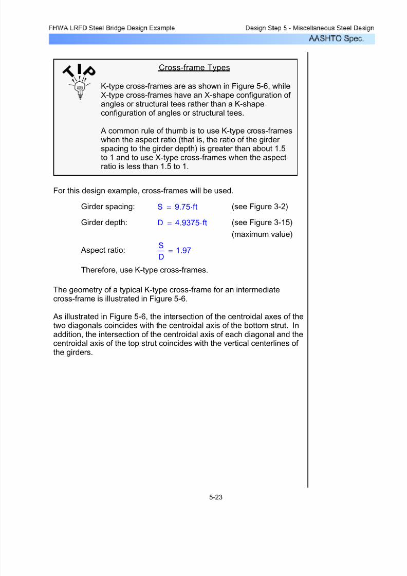
7/29/2019 LRFD steel design.pdf
http://slidepdf.com/reader/full/lrfd-steel-designpdf 325/646
Cross-frame Types
K-type cross-frames are as shown in Figure 5-6, whileX-type cross-frames have an X-shape configuration of angles or structural tees rather than a K-shapeconfiguration of angles or structural tees.
A common rule of thumb is to use K-type cross-frameswhen the aspect ratio (that is, the ratio of the girder spacing to the girder depth) is greater than about 1.5to 1 and to use X-type cross-frames when the aspectratio is less than 1.5 to 1.
For this design example, cross-frames will be used.
Girder spacing: S 9.75 ft⋅= (see Figure 3-2)
Girder depth: D 4.9375 ft⋅= (see Figure 3-15)
(maximum value)
Aspect ratio:S
D1.97=
Therefore, use K-type cross-frames.
The geometry of a typical K-type cross-frame for an intermediate
cross-frame is illustrated in Figure 5-6.
As illustrated in Figure 5-6, the intersection of the centroidal axes of thetwo diagonals coincides with the centroidal axis of the bottom strut. Inaddition, the intersection of the centroidal axis of each diagonal and thecentroidal axis of the top strut coincides with the vertical centerlines of the girders.
5-23

7/29/2019 LRFD steel design.pdf
http://slidepdf.com/reader/full/lrfd-steel-designpdf 326/646
Pw 0.366K=Pw W Lb⋅=
Lb 20 ft⋅=
W 0.0183 Kft
=
C4.6.2.7.1 Pw W Lb⋅= Lb
The horizontal wind force applied to the brace point may then be
computed as specified in C4.6.2.7.1, as follows:
W 0.0183K
ft=W
η γ⋅ PD⋅ d⋅
2=
(maximum value)d 4.9375ft=
(see Design Step 3.17)PD 0.00529 ksf ⋅=
STable 3.4.1-1 (for Strength III Limit State)γ 1.40=
S1.3 η 1.0=
C4.6.2.7.1 Wη γ⋅ PD⋅ d⋅
2=
PD
Based on previous computations in Design Step 3.17 for the negativemoment region, the unfactored wind load is computed as follows:
Figure 5-6 K-Type Cross-frame
9'-9"
Steel Angle or Tee (Typ.)
4'-10 1/2"4'-10 1/2"
5-24

7/29/2019 LRFD steel design.pdf
http://slidepdf.com/reader/full/lrfd-steel-designpdf 327/646
For the design of the cross-frame members, the following checks shouldbe made using the previously computed wind load:
Slenderness•
Axial compression• Flexure about the major axis•Flexure about the minor axis•Flexure and axial compression•
5-25

7/29/2019 LRFD steel design.pdf
http://slidepdf.com/reader/full/lrfd-steel-designpdf 328/646
15Design Step 6.14 - Draw Schematic of Final Bearing Design
12Design Step 6.13 - Design Anchorage for Fixed Bearing
10Design Step 6.12 - Design for Anchorage
9Design Step 6.11 - Check Reinforcement
9Design Step 6.10 - Check Stability
8Design Step 6.9 - Check Rotation or Combined Compressionand Rotation
7Design Step 6.8 - Check Shear Deformation5Design Step 6.7 - Check Compressive Deflection
5Design Step 6.6 - Check Compressive Stress
4Design Step 6.5 - Compute Shape Factor
3Design Step 6.4 - Select Design Method (A or B)
3Design Step 6.3 - Select Preliminary Bearing Properties
2Design Step 6.2 - Select Optimum Bearing Type
2Design Step 6.1 - Obtain Design Criteria
PageTable of Contents
Bearing Design ExampleDesign Step 6
6-1

7/29/2019 LRFD steel design.pdf
http://slidepdf.com/reader/full/lrfd-steel-designpdf 329/646
S14.6.2Selecting the optimum bearing type depends on the load, movement
capabilities, and economics. Refer to STable 14.6.2-1 and SFigure14.6.2-1 for guidance on selecting the most practical bearing type.For the abutment bearing design, a steel-reinforced elastomericbearing was selected. If the loads were considerably larger, potbearings, which are more expensive than elasomeric bearings, wouldbe an option.
Design Step 6.2 - Select Optimum Bearing Type
Strength limit state minimum vertical forcedue to permanent loads (used in DesignStep 6.12)
Psd 67.8K=
Service I limit state total rotation about thetransverse axis (see Figure 6-1)
θsx 0.0121rad=
Service I limit state live load (includingdynamic load allowance)
LLserv 110.4K=
Service I limit state dead loadDLserv 78.4K=
For bearing design, the required design criteria includes:
1. Longitudinal and transverse movement2. Longitudinal, transverse, and vertical rotation3. Longitudinal, transverse, and vertical loads
Most of the above information is typically obtained from thesuperstructure design software output, which is the case for this bearingdesign (first trial of girder design):
ksiK
in2
=K 1000lb=
The following units are defined for use in this design example:
Refer to Design Step 1 for introductory information about this designexample. Additional information is presented about the designassumptions, methodology, and criteria for the entire bridge, includingthe bearing design.
For this bearing design example, an abutment bearing was chosen. Itwas decided that the abutment would have expansion bearings.Therefore, the bearing design will be for an expansion bearing.
Design Step 6.1 - Obtain Design Criteria
6-2
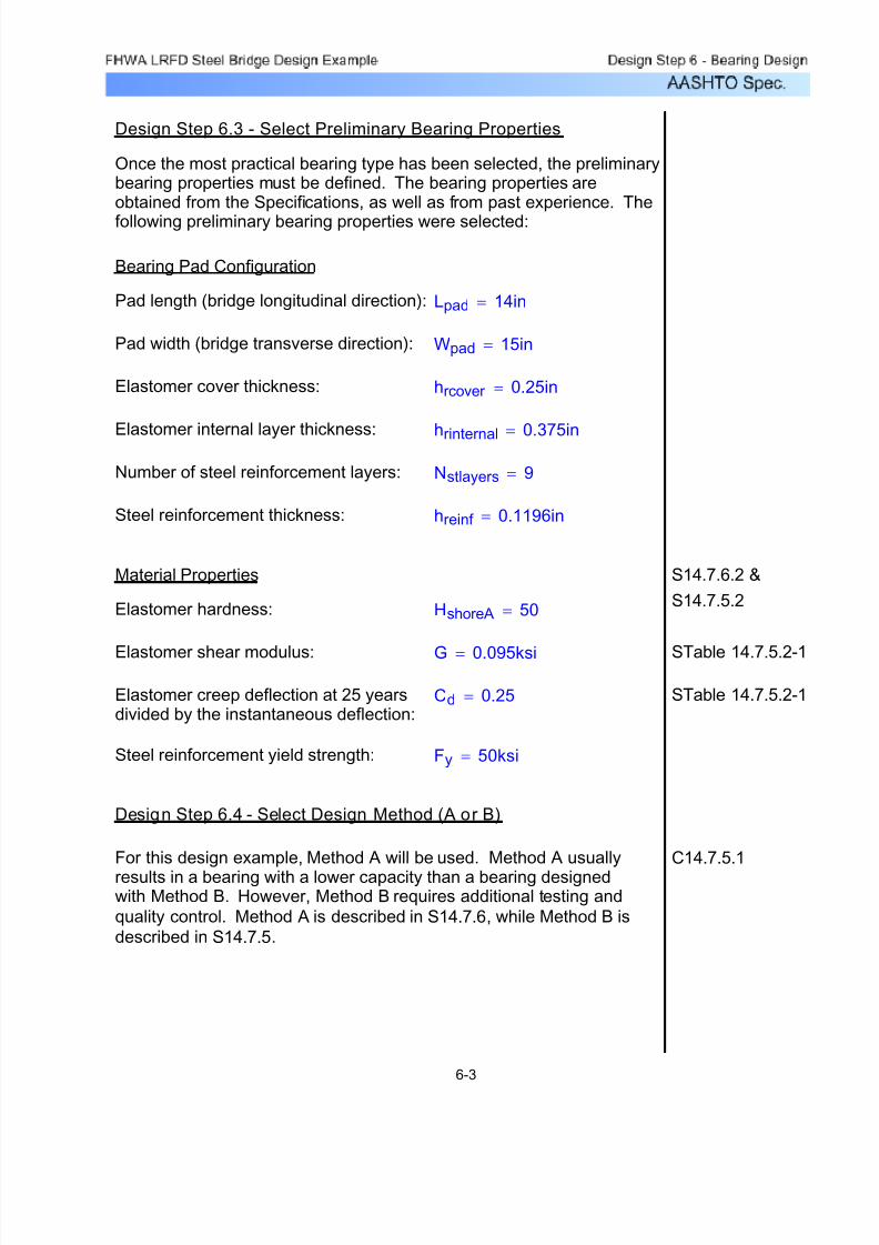
7/29/2019 LRFD steel design.pdf
http://slidepdf.com/reader/full/lrfd-steel-designpdf 330/646
C14.7.5.1For this design example, Method A will be used. Method A usually
results in a bearing with a lower capacity than a bearing designedwith Method B. However, Method B requires additional testing and
quality control. Method A is described in S14.7.6, while Method B is
described in S14.7.5.
Design Step 6.4 - Select Design Method (A or B)
Fy 50ksi=Steel reinforcement yield strength:
STable 14.7.5.2-1Cd 0.25=Elastomer creep deflection at 25 yearsdivided by the instantaneous deflection:
STable 14.7.5.2-1G 0.095ksi=Elastomer shear modulus:
HshoreA 50=Elastomer hardness:S14.7.5.2
S14.7.6.2 &Material Properties
hreinf 0.1196in=Steel reinforcement thickness:
Nstlayers 9=Number of steel reinforcement layers:
hrinternal 0.375in=Elastomer internal layer thickness:
hrcover 0.25in=Elastomer cover thickness:
Wpad 15in=Pad width (bridge transverse direction):
Lpad 14in=Pad length (bridge longitudinal direction):
Bearing Pad Configuration
Once the most practical bearing type has been selected, the preliminarybearing properties must be defined. The bearing properties areobtained from the Specifications, as well as from past experience. The
following preliminary bearing properties were selected:
Design Step 6.3 - Select Preliminary Bearing Properties
6-3
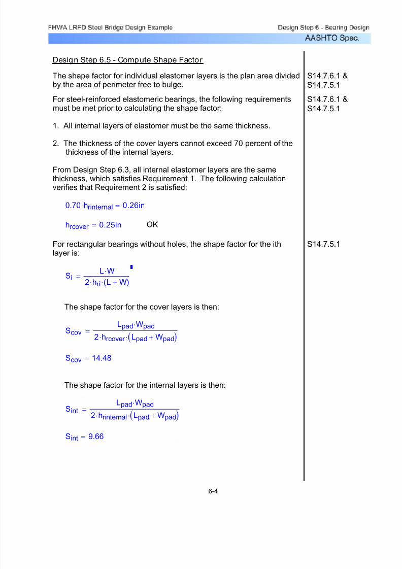
7/29/2019 LRFD steel design.pdf
http://slidepdf.com/reader/full/lrfd-steel-designpdf 331/646
Sint 9.66=
SintLpad Wpad⋅
2 hrinternal⋅ Lpad Wpad+( )⋅=
The shape factor for the internal layers is then:
Scov 14.48=
ScovLpad Wpad⋅
2 hrcover ⋅ Lpad Wpad+( )⋅=
The shape factor for the cover layers is then:
SiL W⋅
2 hri⋅ L W+( )⋅=
S14.7.5.1For rectangular bearings without holes, the shape factor for the ithlayer is:
OKhrcover 0.25in=
0.70 hrinternal⋅ 0.26in=
From Design Step 6.3, all internal elastomer layers are the samethickness, which satisfies Requirement 1. The following calculationverifies that Requirement 2 is satisfied:
S14.7.6.1 &S14.7.5.1
For steel-reinforced elastomeric bearings, the following requirementsmust be met prior to calculating the shape factor:
1. All internal layers of elastomer must be the same thickness.
2. The thickness of the cover layers cannot exceed 70 percent of thethickness of the internal layers.
S14.7.6.1 &
S14.7.5.1
The shape factor for individual elastomer layers is the plan area dividedby the area of perimeter free to bulge.
Design Step 6.5 - Compute Shape Factor
6-4

7/29/2019 LRFD steel design.pdf
http://slidepdf.com/reader/full/lrfd-steel-designpdf 332/646
δ Σεi hri⋅=
S14.7.5.3.3The compressive deflection due to the total load at the service limitstate is obtained from the following equation:
Design Step 6.7 - Check Compressive Deflect ion
σL 0.526ksi=
σL
LLserv
Lpad Wpad⋅( )=
The service average compressive stress due to live load onlywill also be computed at this time. It will be needed in DesignStep 6.11. Again, the service limit state live load value wasobtained from Opis superstructure output.
OK1.0 G⋅ Sint⋅ 0.917ksi=
σs 0.899ksi=
σs
DLserv LLserv+
Lpad Wpad⋅( )=
LLserv 110.4K=Service I limit state live load(including dynamic load allowance):
DLserv 78.4K=Service I limit state dead load:
The compressive stress is taken as the total reaction at one of the abutment bearings for the service limit state divided by theelastomeric pad plan area. The service limit state dead andlive load reactions are obtained from the Opis superstructureoutput. The shape factor used in the above equation should befor the thickest elastomer layer.
σs 1.0 G⋅ S⋅≤andσs 1.0ksi≤
S14.7.6.3.2The compressive stress check limits the compressive stress in theelastomer at the service limit state as follows:
Design Step 6.6 - Check Compressive Stress
6-5

7/29/2019 LRFD steel design.pdf
http://slidepdf.com/reader/full/lrfd-steel-designpdf 333/646
OK0.07hrinternal 0.026in=
δ int1layer 0.015in=
δ int1layer ε int hrinternal⋅=
In order to reduce design steps, the above requirement will bechecked using the deflection calculated for the service limit stateincluding dynamic load allowance. If the compressive deflection isgreater than 0.07hri, then the deflection without dynamic loadallowance would need to be calculated.
S14.7.6.3.3The initial compressive deflection in any layer of a steel-reinforcedelastomeric bearing at the service limit state without dynamic loadallowance shall not exceed 0.07hri.
δtotal 0.175in=
δtotal δ inst δcreep+=
The total deflection is then:
δcreep 0.035in=
δcreep Cd δ inst⋅=
STable 14.7.5.2-1The effects of creep should also be considered. For this designexample, material-specific data is not available. Therefore, calculatethe creep deflection value as follows:
δ inst 0.140in=
S14.7.5.3.3 δ inst 2 ε int⋅ hrcover ⋅ 8 ε int⋅ hrinternal⋅+=
The instantaneous deflection is then:
CTable14.7.5.3.3-1
ε int 0.04=
For this design example, the instantaneous compressive strain
was approximated from CTable 14.7.5.3.3-1 for 50 durometer reinforced bearings using a compressive stress of 0.899 ksi and ashape factor of 9.66.
6-6
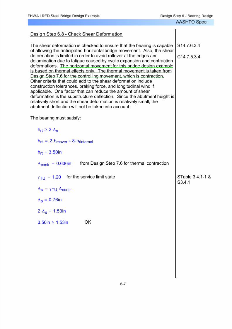
7/29/2019 LRFD steel design.pdf
http://slidepdf.com/reader/full/lrfd-steel-designpdf 334/646
OK3.50in 1.53in≥
2 ∆s⋅ 1.53in=
∆s 0.76in=
∆s γTU ∆contr ⋅=
STable 3.4.1-1 &
S3.4.1
for the service limit stateγTU 1.20=
from Design Step 7.6 for thermal contraction∆contr 0.636in=
hrt 3.50in=
hrt 2 hrcover ⋅ 8 hrinternal⋅+=
hrt 2 ∆s⋅≥
The bearing must satisfy:
C14.7.5.3.4
S14.7.6.3.4The shear deformation is checked to ensure that the bearing is capableof allowing the anticipated horizontal bridge movement. Also, the shear
deformation is limited in order to avoid rollover at the edges anddelamination due to fatigue caused by cyclic expansion and contractiondeformations. The horizontal movement for this bridge design exampleis based on thermal effects only. The thermal movement is taken fromDesign Step 7.6 for the controlling movement, which is contraction.Other criteria that could add to the shear deformation includeconstruction tolerances, braking force, and longitudinal wind if applicable. One factor that can reduce the amount of shear deformation is the substructure deflection. Since the abutment height isrelatively short and the shear deformation is relatively small, theabutment deflection will not be taken into account.
Design Step 6.8 - Check Shear Deformation
6-7

7/29/2019 LRFD steel design.pdf
http://slidepdf.com/reader/full/lrfd-steel-designpdf 335/646
The service rotation due to the total load about the longitudinalaxis is negligible compared to the service rotation about thetransverse axis. Therefore, the check about the longitudinal axiswill be assumed to be negligible and is not computed in thisbearing design example.
OK0.5 G⋅ Sint⋅Lpad
hrinternal
⎛
⎝
⎞
⎠
2
⋅θsx
8 1+( )⋅ 0.859ksi=
n 8 0.5+ 0.5+=
The number of interior layers is:
Construction Tolerance
For spans over approximately 100 feet, it is goodengineering practice to include an additional 0.005radians of rotation about both pad axes to account for construction tolerances.
S14.7.6.3.5dradθsx 0.0121=
The service rotation due to the total load about the transverse axiswas taken from Opis:
σs 0.899ksi=
(associated with rotation about
longitudinal axis)σ
s
0.5G S⋅W
hri
⎛
⎝
⎞
⎠
2
⋅θsz
n⋅≥
and
S14.7.6.3.5d(associated with rotation abouttransverse axis)
σs 0.5G S⋅L
hri
⎛ ⎝
⎞ ⎠
2
⋅θsx
n⋅≥
S14.7.6.3.5Since Design Method A was chosen, combined compression androtation does not need to be checked. The rotation check ensuresthat no point in the bearing undergoes net uplift and is as follows:
Design Step 6.9 - Check Rotation or Combined Compressionand Rotation
6-8
7/29/2019 LRFD steel design.pdf
http://slidepdf.com/reader/full/lrfd-steel-designpdf 336/646
OKhreinf 0.1196in=
3 hmax⋅ σs⋅
Fy0.0202in=
Fy 50ksi=σs 0.899ksi=
hmax 0.375in=hmax hrinternal=
hs
3hmax σs⋅
Fy≥
For the service limit state:
S14.7.5.3.7
S14.7.6.3.7The thickness of the steel reinforcement must be able to sustain thetensile stresses induced by compression in the bearing. Thereinforcement thickness must also satisfy the requirements of the
AASHTO LRFD Bridge Construction Specifications.
Design Step 6.11 - Check Reinforcement
OKhtotal 4.5764in=
htotal 2 hrcover ⋅ 8 hrinternal⋅+ Nstlayers hreinf ⋅+=
The total thickness of the pad based on the preliminarydimensions is:
Wpad
3 5.00in=
Lpad
3 4.67in=
S14.7.6.3.6The total thickness of the pad shall not exceed the least of L/3 or W/3.
Design Step 6.10 - Check Stabi lity
6-9
7/29/2019 LRFD steel design.pdf
http://slidepdf.com/reader/full/lrfd-steel-designpdf 337/646
The controlling shear force is either from Strength III or Strength V:
WL 6.00K=
The shear force due to wind on live load is taken from Table 7-2:
WS 30.69K=
The shear force due to wind on superstructure is taken from Table7-1:
The maximum factored shear force sustained by the deformed padat the strength limit state is obtained from Design Step 7.6, addingwind on superstructure and wind on live load. The maximum shear force will occur when wind is taken at 0 degrees.
taken from Opis outputPsd 67.8K=
S14.7.6.4The bearing pad must be secured against transverse horizontalmovement if the factored shear force sustained by the deformed padat the strength limit state exceeds one-fifth of the minimum verticalforce due to permanent loads, Psd.
Design Step 6.12 - Design for Anchorage
OKhreinf 0.1196in=
2 hmax⋅ σL⋅
∆FTH
0.0164in=
STable 6.6.1.2.5-3∆FTH 24.0ksi=
σL 0.526ksi=
From Design Step 6.6, the service average compressive stressdue to live load only is:
hs
2hmax σL⋅
∆FTH
≥
For the fatigue limit state:
6-10

7/29/2019 LRFD steel design.pdf
http://slidepdf.com/reader/full/lrfd-steel-designpdf 338/646
Since the maximum shear force at the strength limit state does notexceed one-fifth of the minimum vertical force due to permanent deadloads, the pad does not need to be secured against horizontalmovement.
1
5Psd⋅ 13.56K=
Vmax 8.59K=
Vmax max VwindstrIII VwindstrV,( )=Use:
VwindstrV 3.66K=
VwindstrV
γWS WS⋅ γWL WL⋅+( )5
=
STable 3.4.1-1γWL 1.00=
STable 3.4.1-1γWS 0.40=
Factored shear force per bearing for Strength V:
VwindstrIII 8.59K=
VwindstrIII
γWS WS⋅ γWL WL⋅+( )5
=
STable 3.4.1-1γWL 0.00=
STable 3.4.1-1γWS 1.40=
Factored shear force per bearing for Strength III:
6-11

7/29/2019 LRFD steel design.pdf
http://slidepdf.com/reader/full/lrfd-steel-designpdf 339/646
Ab 0.31in2=
Abπ 0.625in( )
2⋅
4=
S6.5.4.2resistance factor for A 307 bolts in shear φs 0.65=
S6.13.2.7for threads excluded from shear planeRn 0.48 Ab⋅ Fub⋅ Ns⋅=
S6.4.3 Assume two 5/8" diameter A 307 bolts with a minimum tensilestrength of 60 ksi:
S14.8.3.1
S6.13.2.7
The factored shear resistance of the anchor bolts per bearing is then:
HEQ 7.84K=
HEQ 0.1 DLserv⋅=
The maximum transverse horizontal earthquake load per bearing isthen:
DLserv 78.4K=
For the controlling girder (interior):
C3.4.1
S3.10.9.2
S14.8.3.1The abutment bearings are expansion in the longitudinal direction butfixed in the transverse direction. Therefore, the bearings must berestrained in the transverse direction. Based on Design Step 6.12,
the expansion bearing pad does not need to be secured againsthorizontal movement. However, based on S3.10.9.2, the horizontalconnection force in the restrained direction cannot be less than 0.1times the vertical reaction due to the tributary permanent load and thetributary live loads assumed to exist during an earthquake. In addition,since all abutment bearings are restrained in the transverse direction,the tributary permanent load can be taken as the reaction at thebearing. Also, γEQ is assumed to be zero. Therefore, no tributary live
loads will be considered. This transverse load will be used to designthe bearing anchor bolts for this design example.
Design Step 6.13 - Design Anchorage for Fixed Bearings
6-12
7/29/2019 LRFD steel design.pdf
http://slidepdf.com/reader/full/lrfd-steel-designpdf 340/646
P1bolt 3.92K=
P1boltHEQ
2=
The transverse load per anchor bolt is then:
HEQ 7.84K=
The total transverse horizontal load is:
Stressbrg 1.78ksi=
Stressbrg φb 0.85⋅ 4ksi( )⋅ m⋅=
S5.5.4.2.1for bearing on concreteφb 0.70=
(conservative assumption)m 0.75= Assume:
Stressbrg φb 0.85⋅ f c⋅ m⋅=
Stressbrg
φb Pn⋅
A1=
S5.7.5φb Pn⋅ φb 0.85⋅ f c⋅ A1⋅ m⋅=
S14.8.3.1
C14.8.3.1
Once the anchor bolt quantity and size are determined, the anchor bolt length must be computed. As an approximation, the bearingstress may be assumed to vary linearly from zero at the end of theembedded length to its maximum value at the top surface of the
concrete. The bearing resistance of the concrete is based onS5.7.5.
OKRr HEQ≥
Rr 11.49K=Rr φs Rn⋅=
Rn 17.67K=Rn 0.48 Ab⋅ Fub⋅ Ns⋅=
(number of bolts)Ns 2=
Fub 60ksi=
6-13

7/29/2019 LRFD steel design.pdf
http://slidepdf.com/reader/full/lrfd-steel-designpdf 341/646
Using the bearing stress approximation from above, the requiredanchor bolt area resisting the transverse horizontal load can becalculated.
A1P1bolt
Stressbrg 0+2
⎛ ⎝
⎞ ⎠
=
A1 4.39in2=
A1 is the product of the anchor bolt diameter and the length theanchor bolt is embedded into the concrete pedestal/beam seat.Since we know the anchor bolt diameter, we can now solve for therequired embedment length.
Lembed A10.625in
=
Lembed 7.03in=
Individual states and agencies have their own minimum anchor boltembedment lengths. For this design example, a minimum of 12 incheswill be used.
Use: Lembed 12.0in=
6-14

7/29/2019 LRFD steel design.pdf
http://slidepdf.com/reader/full/lrfd-steel-designpdf 342/646
Design Step 6.14 - Draw Schematic of Final Bearing Design
Pad width
90.0°
15.00 in.
1 4 . 0 0 i n .
P a d l e n g t h
L Girder (longitudinal axis)C
L Bearing
(transverse
axis)
C
Figure 6-1 Bearing Pad Plan View
15.00 in.
9 - Steel reinf. layers @ 0.1196 in. thickness each
0.25 in. thickness (Typ. - top & bottom layer)
0.375 in. thickness (Typ. - internal layers)
1/8 in. (Typ.)
4 . 5 7 6 4
i n .
Figure 6-2 Bearing Pad Elevation View
6-15

7/29/2019 LRFD steel design.pdf
http://slidepdf.com/reader/full/lrfd-steel-designpdf 343/646
4 . 5 7 6 4
i n .
12.00in.
5/8" Diameter
A 307 Bolt
(Typ.)
Embedment(Typ.)
Figure 6-3 Anchor Bolt Embedment
6-16

7/29/2019 LRFD steel design.pdf
http://slidepdf.com/reader/full/lrfd-steel-designpdf 344/646
63
Design Step 7.11 - Design Abutment Footing 71
Design Step 7.12 - Draw Schematic of Final Abutment Design 97
Design Step 7.2 - Select Optimum Wingwall Type 98
Design Step 7.3 - Select Preliminary Wingwall Dimensions 98
Design Step 7.4 - Compute Dead Load Effects 99Design Step 7.5 - Compute Live Load Effects 101
Design Step 7.6 - Compute Other Load Effects 101
Design Step 7.7 - Analyze and Combine Force Effects 104
Design Step 7.9 - Design Wingwall Stem 111
Design Step 7.12 - Draw Schematic of Final Wingwall Design 119
Abutment and Wingwall Design ExampleDesign Step 7
Table of Contents
Page
Design Step 7.1 - Obtain Design Criteria 2
Design Step 7.2 - Select Optimum Abutment Type 5
Design Step 7.3 - Select Preliminary Abutment Dimensions 5
Design Step 7.4 - Compute Dead Load Effects 6
Design Step 7.5 - Compute Live Load Effects 8
Design Step 7.6 - Compute Other Load Effects 10
Design Step 7.7 - Analyze and Combine Force Effects 27
Design Step 7.8 - Check Stability and Safety Requirements 54
Design Step 7.9 - Design Abutment Backwall 54
Design Step 7.10 - Design Abutment Stem
7-1

7/29/2019 LRFD steel design.pdf
http://slidepdf.com/reader/full/lrfd-steel-designpdf 345/646
Design Step 7.1 - Obtain Design Criteria
This abutment and wingwall design example is based on AASHTO
LRFD Bridge Design Specifications (through 2002 interims). The
design methods presented throughout the example are meant to be themost widely used in general bridge engineering practice. The examplecovers the abutment backwall, stem, and footing design, using pileloads from Design Step P, Pile Foundation Design Example. Thewingwall design focuses on the wingwall stem only. All applicable loadsthat apply to the abutment and wingwall are either taken from designsoftware or calculated herein.
The wingwall design utilizes the same flowchart as the abutment.Design Step 7.1 is shared by both the abutment and wingwall. After Design Step 7.1, Design Steps 7.2 through 7.12 are for the abutment.For the wingwall, any Design Steps from 7.2 through 7.12 that apply to
the wingwall follow at the end of the abutment design steps. For example, there are two Design Steps 7.2 - one for the abutment andone for the wingwall (after Design Step 7.12 of the abutment).
Refer to Design Step 1 for introductory information about this designexample. Additional information is presented about the designassumptions, methodology, and criteria for the entire bridge, includingthe abutments and wingwalls.
In order to begin the design, the abutment and wingwall properties aswell as information about the superstructure that the abutment supports
is required.
The following units are defined for use in this design example:
K 1000lb= kcf K
ft3
= ksiK
in2
= ksf K
ft2
= klf K
ft=
It should be noted that the superstructure loads and plate girder dimensions used in this design step are based on the first trial of thegirder design.
7-2

7/29/2019 LRFD steel design.pdf
http://slidepdf.com/reader/full/lrfd-steel-designpdf 346/646
Stem back cover: Cover s 2.5in= STable 5.12.3-1
Footing top cover: Cover ft 2.0in= STable 5.12.3-1
Footing bottom cover: Cover fb 3.0in= STable 5.12.3-1
Backwall back cover - Assuming that the backwall will be subject to
deicing salts, the cover is set at 2.5 inches.
STable 5.12.3-1
Stem cover - The stem cover is set at 2.5 inches. This will allow the
vertical flexure reinforcement in the stem to be lapped with the verticalback face reinforcement in the backwall. Also, it is assumed that thestem may be exposed to deicing salts due to the abutment having anexpansion joint.
STable 5.12.3-1
Footing top cover - The footing top cover is set at 2.0 inches. STable 5.12.3-1
Footing bottom cover - Since the footing bottom is cast directly
against the earth, the footing bottom cover is set at 3.0 inches.
STable 5.12.3-1
Material properties:
Concrete density: Wc 0.150kcf = STable 3.5.1-1
Concrete 28-daycompressive strength:
f'c
4.0ksi= S5.4.2.1
SC5.4.2.1
STable C5.4.2.1-1
Reinforcementstrength:
f y 60ksi= S5.4.3
Reinforcing steel cover requirements:
Backwall back cover: Cover b 2.5in= STable 5.12.3-1
7-3

7/29/2019 LRFD steel design.pdf
http://slidepdf.com/reader/full/lrfd-steel-designpdf 347/646
Lwing 20.5ft=Wingwall length:
Labut 46.875ft=Abutment length:
S11.6.1.4 Abutment and wingwall length
use height at 3/4point
hwwstem 20.75ft=Wingwall stem design height:
hstem 22ft=Abutment stem height:
S2.3.3.2 Abutment and wingwall height
Superstructure data - The above superstructure information was
taken from Design Steps 1 and 2.
Wdeck 46.875ft=Out-to-out deck width:
Wpar 0.53K
ft=Parapet weight (each):
Hpar 3.5ft=Parapet height:
Lspan 120ft=Span length:N 5=
Number of girders:
S 9.75ft=Girder spacing:
Relevant superstructure data:
7-4
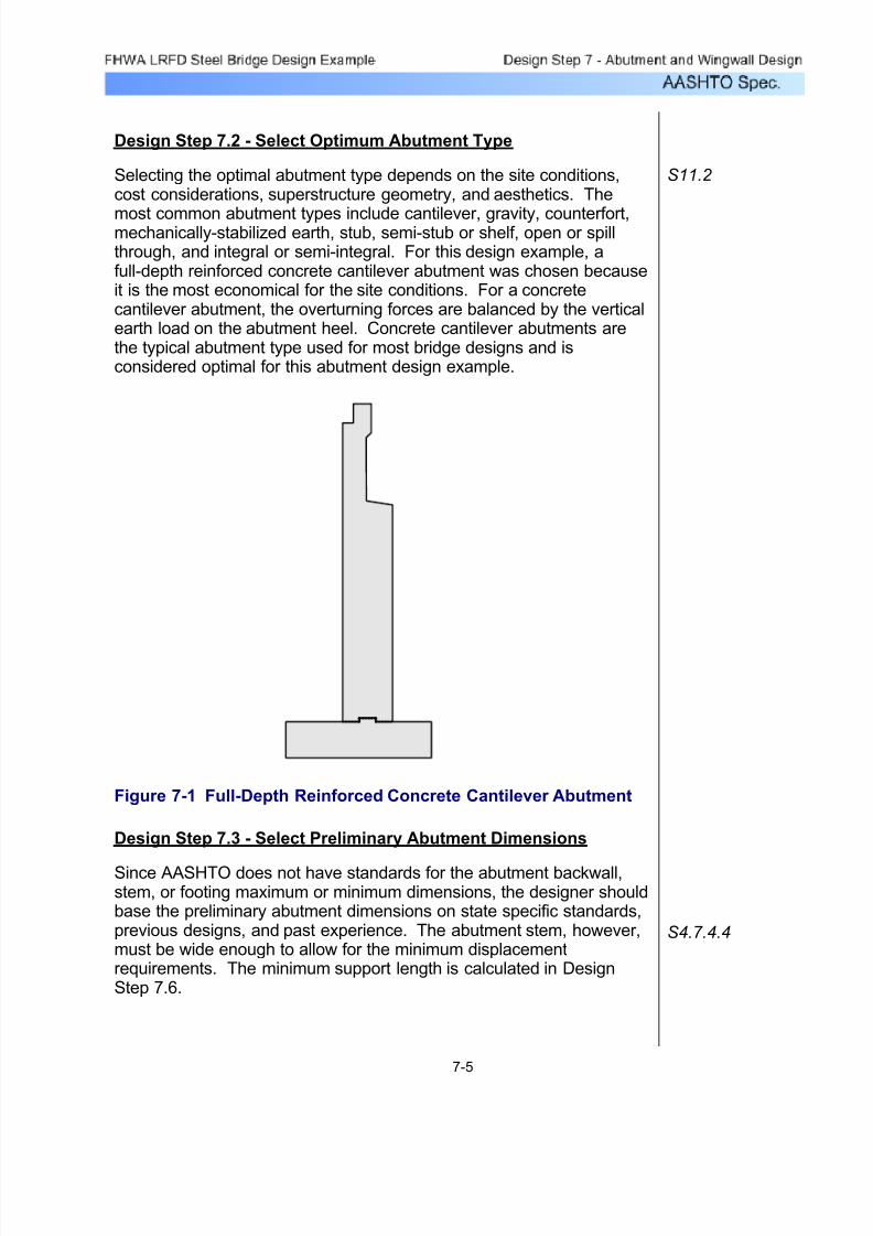
7/29/2019 LRFD steel design.pdf
http://slidepdf.com/reader/full/lrfd-steel-designpdf 348/646
Design Step 7.2 - Select Optimum Abutment Type
Selecting the optimal abutment type depends on the site conditions,cost considerations, superstructure geometry, and aesthetics. The
most common abutment types include cantilever, gravity, counterfort,mechanically-stabilized earth, stub, semi-stub or shelf, open or spillthrough, and integral or semi-integral. For this design example, afull-depth reinforced concrete cantilever abutment was chosen becauseit is the most economical for the site conditions. For a concretecantilever abutment, the overturning forces are balanced by the verticalearth load on the abutment heel. Concrete cantilever abutments arethe typical abutment type used for most bridge designs and isconsidered optimal for this abutment design example.
S11.2
Figure 7-1 Full-Depth Reinforced Concrete Cantilever Abutment
Design Step 7.3 - Select Preliminary Abutment Dimensions
Since AASHTO does not have standards for the abutment backwall,stem, or footing maximum or minimum dimensions, the designer shouldbase the preliminary abutment dimensions on state specific standards,previous designs, and past experience. The abutment stem, however,must be wide enough to allow for the minimum displacementrequirements. The minimum support length is calculated in DesignStep 7.6.
S4.7.4.4
7-5

7/29/2019 LRFD steel design.pdf
http://slidepdf.com/reader/full/lrfd-steel-designpdf 349/646
The following figure shows the preliminary dimensions for this abutmentdesign example.
7 ' - 0 "
3'-6"
2 ' - 0 "
4 "
1'-3"9"
1 ' - 4 "
10'-3"
2 ' - 6 "
4"
5%
1 5 ' - 0 "
2'-9"4'-0"
Figure 7-2 Preliminary Abutment Dimensions
For sealed expansion joints, slope the top surface of the abutment(excluding bearing seats) a minimum of 5% towards the edge.
S2.5.2.1.2
Design Step 7.4 - Compute Dead Load Effects
Once the preliminary abutment dimensions are selected, thecorresponding dead loads can be computed. Along with the abutmentdead loads, the superstructure dead loads must be computed. Thesuperstructure dead loads acting on the abutment will be given based onthe superstructure output from the software used to design thesuperstructure. The dead loads are calculated on a per foot basis.
Also, the dead loads are calculated assuming the beam seat is level.
S3.5.1
7-6

7/29/2019 LRFD steel design.pdf
http://slidepdf.com/reader/full/lrfd-steel-designpdf 350/646
DLstem 7.88K
ft=
DLstem 15ft 3.5⋅ ft Wc⋅=
Stem dead load:
DLbw 1.71 Kft
=
DLbw 1.25ft 1.33⋅ ft( ) 2.0ft 0.67⋅ ft( )+2ft 1.67ft+
2
⎛ ⎝
⎞ ⎠
0.33⋅ ft⎡⎣
⎤⎦
4.67ft 1.67⋅ ft( )++
...⎡
⎣
⎤
⎦
Wc⋅=
Backwall dead load:
RDWtot 1.20K
ft=
RDWtot2 RDWfascia⋅( ) 3RDWinterior ( )+
Labut=
RDCtot 7.66K
ft=
RDCtot2 RDCfascia⋅( ) 3 RDCinterior ⋅( )+
Labut=
As previously stated, the superstructure dead load reactions must beconverted into a load applied to a one-foot strip of abutment. This isaccomplished by adding the two fascia girder dead load reactions withthe three interior girder dead load reactions and then dividing by theabutment length.
RDWinterior 11.24K=RDCinterior 73.51K=
Interior girder:
RDWfascia 11.24K=RDCfascia 69.25K=
Fascia girder:
The superstructure dead load reactions per bearing were obtained fromtrial one of the steel grider design and are as follows.
7-7

7/29/2019 LRFD steel design.pdf
http://slidepdf.com/reader/full/lrfd-steel-designpdf 351/646
RLLbw 2.81K
ft=
RLLbw6 16 K⋅( )⋅ 1 IM+( )⋅ 3 0.64 klf ⋅( )⋅ 2.0 ft⋅( )⋅+[ ]
Labut=
For this design example, the backwall live load is computed byplacing three design truck axles along the abutment and calculatingthe load on a per foot basis including impact and the multiplepresence factor. This load is applied to the entire length of abutment backwall and is assumed to act at the front top corner (bridge side) of the backwall. This load is not applied, however,
when designing the abutment stem or footing.
STable 3.6.1.1.2-1m3 0.85=Multiple presence factor, m (3 lanes)
STable 3.6.1.1.2-1m2 1.00=Multiple presence factor, m (2 lanes)STable 3.6.1.1.2-1m1 1.20=Multiple presence factor, m (1 lane)
STable 3.6.2.1-1IM 0.33=Dynamic load allowance, IM
The live load effects were also obtained from trial one of the girder design. The reactions for one girder are given as unfactored, withoutimpact, and without distribution factors. The given reactions areconverted into one loaded lane and then converted into a per foot load.
Design Step 7.5 - Compute Live Load Effects
DLearth 10.56K
ft=
DLearth 22ft 4⋅ ft γs⋅=
STable 3.5.1-1use average of loose and compacted gravelγs 0.120kcf =
Earth dead load:
DLftg 3.84K
ft=
DLftg 10.25ft 2.5⋅ ft Wc⋅=
Footing dead load:
7-8
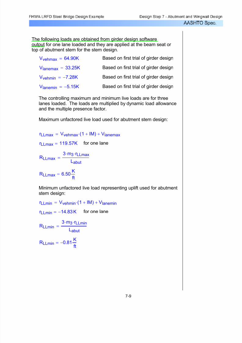
7/29/2019 LRFD steel design.pdf
http://slidepdf.com/reader/full/lrfd-steel-designpdf 352/646
RLLmin 0.81− Kft
=
RLLmin3 m3⋅ r LLmin⋅
Labut=
for one laner LLmin 14.83− K=
r LLmin Vvehmin 1 IM+( )⋅ Vlanemin+=
Minimum unfactored live load representing uplift used for abutmentstem design:
RLLmax 6.50K
ft
=
RLLmax3 m3⋅ r LLmax⋅
Labut=
for one laner LLmax 119.57K=
r LLmax Vvehmax 1 IM+( )⋅ Vlanemax+=
Maximum unfactored live load used for abutment stem design:
The controlling maximum and minimum live loads are for threelanes loaded. The loads are multiplied by dynamic load allowanceand the multiple presence factor.
Based on first trial of girder designVlanemin 5.15− K=
Based on first trial of girder designVvehmin 7.28− K=
Based on first trial of girder designVlanemax 33.25K=Based on first trial of girder designVvehmax 64.90K=
The following loads are obtained from girder design softwareoutput for one lane loaded and they are applied at the beam seat or top of abutment stem for the stem design.
7-9

7/29/2019 LRFD steel design.pdf
http://slidepdf.com/reader/full/lrfd-steel-designpdf 353/646
Since the abutment has expansion bearings, the braking force does notapply at the abutment. The entire braking force is resisted by the fixedbearings located at the pier. Braking force calculations are provided inDesign Step 8.
Braking Force
Other load effects that need to be computed include braking force, windloads, earthquake loads, earth pressure, live load surcharge, andtemperature loads.
Design Step 7.6 - Compute Other Load Effects
RLLmin1 0.68−K
ft=
RLLmin13 m3⋅ r LLmin1⋅
Labut=
for one lane loadedr LLmin1 12.43− K=
r LLmin1 Vvehmin Vlanemin+=
Minimum unfactored vehicle load used for abutment footing design:
RLLmax1 5.34
K
ft=
RLLmax13 m3⋅ r LLmax1⋅
Labut=
for one lane loadedr LLmax1 98.15K=
r LLmax1 Vvehmax Vlanemax+=
Maximum unfactored live load used for abutment footing design:
S3.6.2.1
The following loads are applied at the beam seat or top of abutment stem for the footing design. The loads do not includedynamic load allowance, but do include the multiple presencefactor.
7-10
- Pier
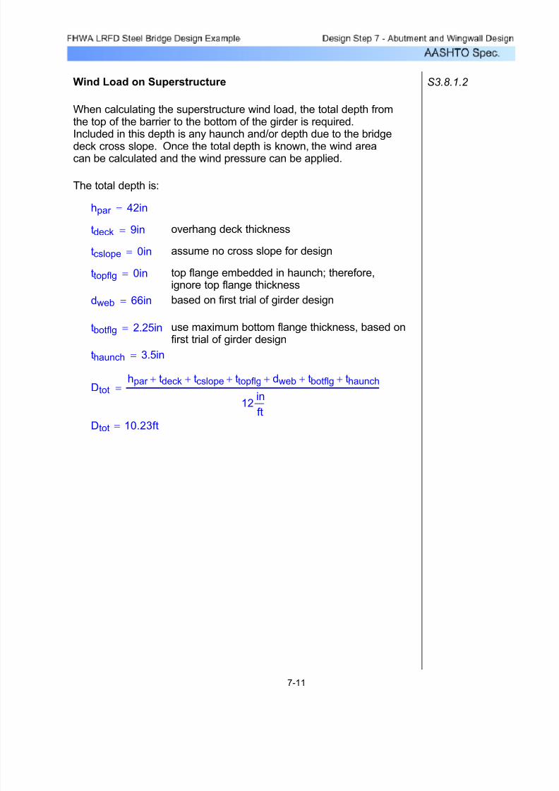
7/29/2019 LRFD steel design.pdf
http://slidepdf.com/reader/full/lrfd-steel-designpdf 354/646
Dtot 10.23ft=
Dtothpar tdeck+ tcslope+ ttopflg+ dweb+ tbotflg+ thaunch+
12in
ft
=
thaunch 3.5in=
use maximum bottom flange thickness, based onfirst trial of girder design
tbotflg 2.25in=
based on first trial of girder designdweb 66in=
top flange embedded in haunch; therefore,ignore top flange thicknessttopflg 0in=
assume no cross slope for designtcslope 0in=
overhang deck thicknesstdeck 9in=
hpar 42in=
The total depth is:
When calculating the superstructure wind load, the total depth fromthe top of the barrier to the bottom of the girder is required.
Included in this depth is any haunch and/or depth due to the bridgedeck cross slope. Once the total depth is known, the wind areacan be calculated and the wind pressure can be applied.
S3.8.1.2 Wind Load on Superstructure
7-11

7/29/2019 LRFD steel design.pdf
http://slidepdf.com/reader/full/lrfd-steel-designpdf 355/646
S3.8.1.2.2 The wind load from the superstructure acting on the abutmentdepends on the attack angle of the wind. Two wind load calculations
are provided for two different wind attack angles. All wind loads aretabulated in Table 7-1 for the various attack angles. The attack angleis measured from a line perpendicular to the girder longitudinal axis.The wind pressure can be applied to either superstructure face. Thebase wind pressures for the superstructure for various attack angles
are given in STable 3.8.1.2.2-1. Since the abutment has expansionbearings, the longitudinal component of the wind load onsuperstructure will not be resisted by the abutment and is notrequired to be calculated. The fixed pier will resist the longitudinalwind component.
, which is greater than 0.30 klf Windtotal 0.51K
ft=
Windtotal 0.050ksf Dtot⋅=
S3.8.1.2.1 Also, the total wind loading on girders must be greater than or equalto 0.30 klf:
PD PB=
PD PB100mph
100mph
⎛ ⎝
⎞ ⎠
2
⋅=or PD PBVDZ
VB
⎛
⎝
⎞
⎠
2
⋅=
S3.8.1.2.1 From this, the design wind pressure is equal to the base windpressure:
VDZ VB=
mphVB 100=
S3.8.1.1 Since the abutment is less than 30 feet in height, the design windvelocity, VDZ, does not have to be adjusted and is equal to the basewind velocity.
Awsuper 613.75ft2=
Awsuper Dtot Lwind⋅=
The wind area is:
Lwind 60ft=
The wind load on the abutment from the superstructure will befrom one-half of one span length or:
7-12
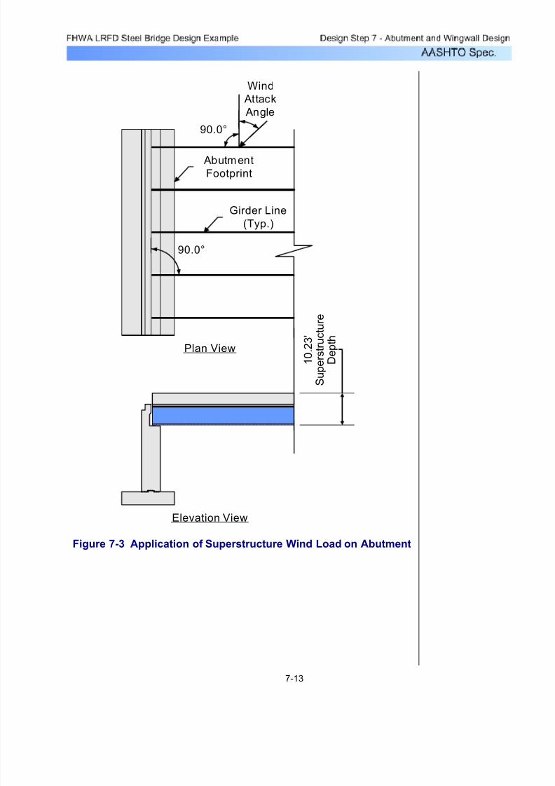
7/29/2019 LRFD steel design.pdf
http://slidepdf.com/reader/full/lrfd-steel-designpdf 356/646
Plan View
Wind
Attack
Angle
Elevation View
Girder Line
(Typ.)
1 0
. 2 3 '
S u p e r s
t r u c
t u r e
D e p
t h
90.0°
90.0°
Abutment
Footprint
Figure 7-3 Application of Superstructure Wind Load on Abutment
7-13

7/29/2019 LRFD steel design.pdf
http://slidepdf.com/reader/full/lrfd-steel-designpdf 357/646
The wind loads acting on the exposed portion of the abutment front andend elevations are calculated from a base wind pressure of 0.040 ksf.These loads act simultaneously with the superstructure wind loads.
S3.8.1.2.3Wind Load on Abutment (Substructure)
Table 7-1 Abutment Design Wind Loads from Superstructurefor Various Wind Attack Angles
* Provided but not applicable due to expansion bearings at
abutment.
45 20.25 9.82
60 10.43 11.66
15 27.01 3.68
30 25.16 7.37
Degrees Kips Kips0 30.69 0.00
Abutment Design Wind Loads from
Superstructure
Wind Attack
Angle
Bridge
Transverse Axis
Bridge *
Longitudinal Axis
not applicable due to expansionbearings at abutment
WSsuperlong60 11.66K=
WSsuperlong60 Awsuper 0.019⋅ ksf =WSsupertrans60 10.43K=
WSsupertrans60 Awsuper 0.017⋅ ksf =
STable 3.8.1.2.2-1For a wind attack angle of 60 degrees, the superstructure wind loadsacting on the abutment are:
not applicable due to expansionbearings at abutment
WSsuperlong0 0.00K=
WSsuperlong0 Awsuper 0.000⋅ ksf =
WSsupertrans0 30.69K=
WSsupertrans0 Awsuper 0.050⋅ ksf =
STable 3.8.1.2.2-1For a wind attack angle of 0 degrees, the superstructure wind loadsacting on the abutment are:
7-14

7/29/2019 LRFD steel design.pdf
http://slidepdf.com/reader/full/lrfd-steel-designpdf 358/646
Since all wind loads acting on the abutment front face decrease themaximum longitudinal moment, all abutment front face wind loads willbe conservatively ignored.
The abutment exposed end elevation wind area is:
Awsubend 3.5ft( ) 22ft( )⋅=
Awsubend 77.00ft2=
Two wind load calculations for the abutment end elevation are shownbelow for a wind attack angle of zero and sixty degrees. All other windattack angles do not control and are not shown.
For a wind attack angle of 0 degrees, the wind loads acting on the
abutment end elevation are:
WSsubtransend0 Awsubend 0.040 ksf ⋅ cos 0 deg⋅( )⋅( )⋅=
WSsubtransend0 3.08K=
WSsublongend0 Awsubend 0.040ksf sin 0deg( )⋅( )⋅=
WSsublongend0 0.00K=
7-15
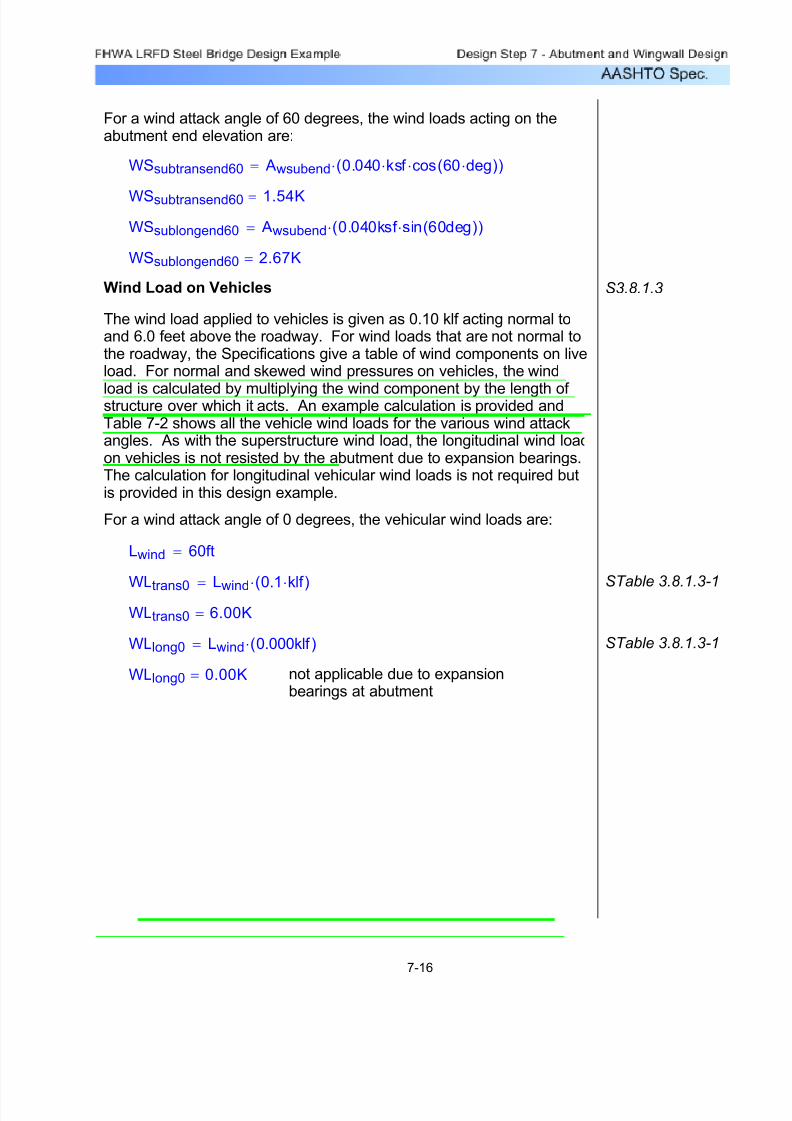
7/29/2019 LRFD steel design.pdf
http://slidepdf.com/reader/full/lrfd-steel-designpdf 359/646
not applicable due to expansionbearings at abutment
WLlong0 0.00K=
STable 3.8.1.3-1WLlong0 Lwind 0.000klf ( )⋅=
WLtrans0 6.00K=STable 3.8.1.3-1WLtrans0 Lwind 0.1 klf ⋅( )⋅=
Lwind 60ft=
For a wind attack angle of 0 degrees, the vehicular wind loads are:
The wind load applied to vehicles is given as 0.10 klf acting normal toand 6.0 feet above the roadway. For wind loads that are not normal tothe roadway, the Specifications give a table of wind components on liveload. For normal and skewed wind pressures on vehicles, the wind
load is calculated by multiplying the wind component by the length of structure over which it acts. An example calculation is provided andTable 7-2 shows all the vehicle wind loads for the various wind attackangles. As with the superstructure wind load, the longitudinal wind loadon vehicles is not resisted by the abutment due to expansion bearings.The calculation for longitudinal vehicular wind loads is not required butis provided in this design example.
S3.8.1.3Wind Load on Vehicles
WSsublongend60 2.67K=
WSsublongend60 Awsubend 0.040ksf sin 60deg( )⋅( )⋅=
WSsubtransend60 1.54K=
WSsubtransend60 Awsubend 0.040 ksf ⋅ cos 60 deg⋅( )⋅( )⋅=
For a wind attack angle of 60 degrees, the wind loads acting on theabutment end elevation are:
7-16
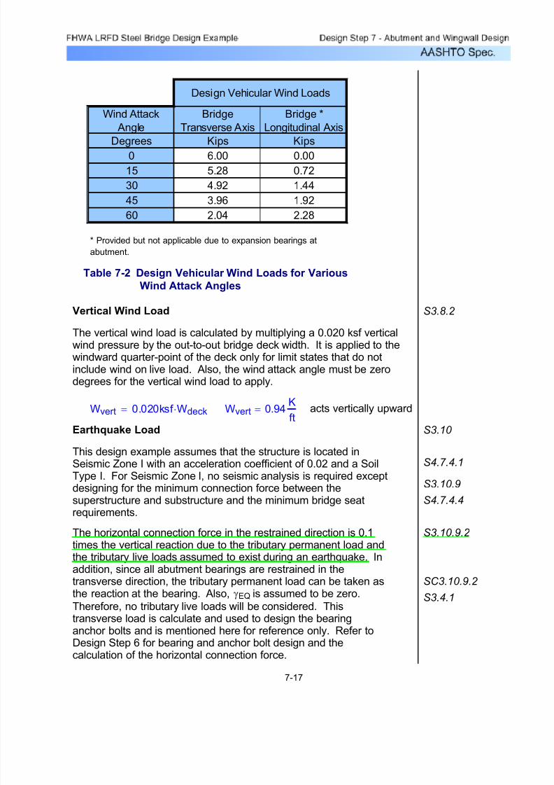
7/29/2019 LRFD steel design.pdf
http://slidepdf.com/reader/full/lrfd-steel-designpdf 360/646
S3.4.1
SC3.10.9.2
S3.10.9.2 The horizontal connection force in the restrained direction is 0.1
times the vertical reaction due to the tributary permanent load andthe tributary live loads assumed to exist during an earthquake. Inaddition, since all abutment bearings are restrained in thetransverse direction, the tributary permanent load can be taken asthe reaction at the bearing. Also, γEQ is assumed to be zero.
Therefore, no tributary live loads will be considered. Thistransverse load is calculate and used to design the bearinganchor bolts and is mentioned here for reference only. Refer toDesign Step 6 for bearing and anchor bolt design and thecalculation of the horizontal connection force.
S4.7.4.4
S3.10.9
S4.7.4.1This design example assumes that the structure is located inSeismic Zone I with an acceleration coefficient of 0.02 and a SoilType I. For Seismic Zone I, no seismic analysis is required exceptdesigning for the minimum connection force between thesuperstructure and substructure and the minimum bridge seatrequirements.
S3.10 Earthquake Load
acts vertically upwardWvert 0.94
K
ft=Wvert 0.020ksf Wdeck⋅=
The vertical wind load is calculated by multiplying a 0.020 ksf verticalwind pressure by the out-to-out bridge deck width. It is applied to thewindward quarter-point of the deck only for limit states that do notinclude wind on live load. Also, the wind attack angle must be zerodegrees for the vertical wind load to apply.
S3.8.2 Vertical Wind Load
Table 7-2 Design Vehicular Wind Loads for VariousWind Attack Angles
Design Vehicular Wind Loads
Wind Attack
Angle
Bridge
Transverse Axis
Bridge *
Longitudinal Axis
Degrees Kips Kips
0 6.00 0.00
15 5.28 0.72
30 4.92 1.44
* Provided but not applicable due to expansion bearings at
abutment.
45 3.96 1.92
60 2.04 2.28
7-17

7/29/2019 LRFD steel design.pdf
http://slidepdf.com/reader/full/lrfd-steel-designpdf 361/646
Figure 7-4 Minimum Support Length Required
3'-6"
3"
N=15"
STable 4.7.4.4-1Since the selected preliminary abutment dimensions in Design Step7.3 leave 18 inches as a support length, this design example will use100 percent of the minimum support length.
inN 15=UseinN 14.56=
N 8 0.02L+ 0.08H+( ) 1 0.000125S2+( )⋅=
degS 0=ftH 22=ftL 240=
S4.7.4.4N 8 0.02L+ 0.08H+( ) 1 0.000125S2+( )⋅=
Minimum support length required:
STable 4.7.4.4-1
S4.7.4.4
From S4.7.4.3, for Seismic Zone I, no seismic analysis is required.Therefore, the minimum displacement requirement must be obtainedfrom a percentage of the empirical seat width. The percentage of theminimum support length, N, is based on Seismic Zone I, an
acceleration coefficient of 0.02, and Soil Type I. From the aboveinformation, 50 percent or greater of the minimum support length isrequired.
7-18

7/29/2019 LRFD steel design.pdf
http://slidepdf.com/reader/full/lrfd-steel-designpdf 362/646
p 0.25ksf =
p ka γs⋅ z⋅=
backwall heightz 7ft=
STable 3.5.1-1use average of loose and compacted gravelγs
0.120kcf =
obtained from geotechnical informationka 0.3=
Bottom of backwall lateral earth load:
p ka γs⋅ z⋅=
S3.11.5.1To obtain the lateral loads due to basic earth pressure, the earthpressure (p) must first be calculated from the following equation.
S3.11.5 Loads due to basic lateral earth pressure:
S11.6.6
S3.11.3The water table is considered to be below the bottom of footing for thisdesign example. Therefore, the effect of hydrostatic water pressuredoes not need to be added to the earth pressure. Hydrostatic water pressure should be avoided if possible in all abutment and retaining walldesign cases through the design of an appropriate drainage system.Some ways that can reduce or eliminate hydrostatic water pressureinclude the use of pipe drains, gravel drains, perforated drains,geosynthetic drains, or backfilling with crushed rock. It should be notedthat the use of weep holes, or drains at the wall face, do not assure fullydrained conditions.
S3.11.6 S3.11.5
The earth loads that need to be investigated for this design exampleinclude loads due to basic lateral earth pressure, loads due to
uniform surcharge, and live load surcharge loads.
S3.11Earth Loads
7-19

7/29/2019 LRFD steel design.pdf
http://slidepdf.com/reader/full/lrfd-steel-designpdf 363/646
7 ' - 0 "
3'-6"
10'-3" 2 ' - 6 "
1 5 ' - 0 "
2 ' - 4 "
REHbw
p
Figure 7-5 Backwall Design Earth Pressure
Once the lateral earth pressure is calculated, the lateral loaddue to the earth pressure can be calculated. This load actsat a distance of H/3 from the bottom of the section beinginvestigated. S3.11.5.1
SC3.11.5.1
hbkwll 7ft=
REHbw1
2
⎛ ⎝
⎞ ⎠
p⋅ hbkwll⋅=
REHbw 0.88K
ft=
7-20

7/29/2019 LRFD steel design.pdf
http://slidepdf.com/reader/full/lrfd-steel-designpdf 364/646
REHstem 8.71K
ft=
REHstem1
2
⎛ ⎝
⎞ ⎠
p⋅ hstem⋅=
SC3.11.5.1S3.11.5.1
Once the lateral earth pressure is calculated, the lateral loaddue to the earth pressure can be calculated. This load acts
at a distance of H/3 from the bottom of the section beinginvestigated.
Figure 7-6 Abutment Stem Design Earth Pressure
7 ' - 0 "
3'-6"
10'-3" 2 ' - 6 "
1 5 ' - 0 "
7 ' - 4 "
REHstem
p
p 0.79ksf =
p ka γs⋅ z⋅=
height used for maximum moment atbottom of abutment stem
z 22ft=
STable 3.5.1-1use average of loose and compacted gravelγs 0.120kcf =
obtained from geotechnical informationka 0.3=
Bottom of abutment stem lateral earth load:
7-21
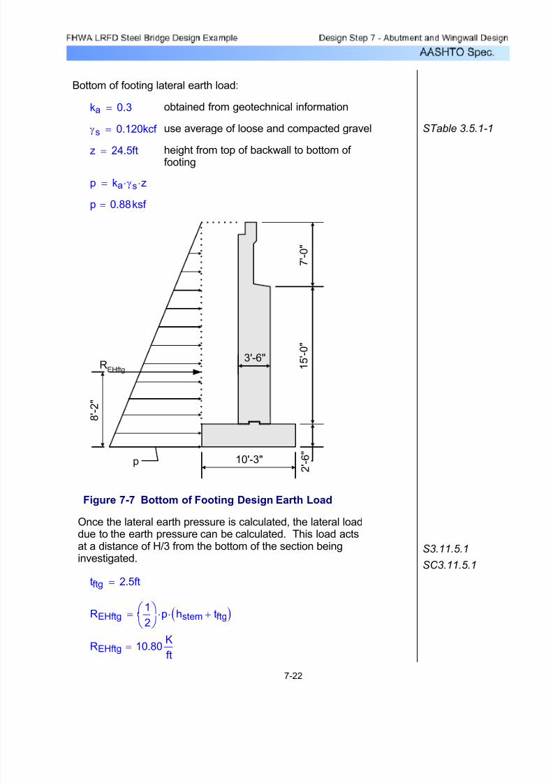
7/29/2019 LRFD steel design.pdf
http://slidepdf.com/reader/full/lrfd-steel-designpdf 365/646
REHftg 10.80K
ft=
REHftg1
2
⎛ ⎝
⎞ ⎠
p⋅ hstem tftg+( )⋅=
tftg 2.5ft=
SC3.11.5.1S3.11.5.1
Once the lateral earth pressure is calculated, the lateral loaddue to the earth pressure can be calculated. This load acts
at a distance of H/3 from the bottom of the section beinginvestigated.
Figure 7-7 Bottom of Footing Design Earth Load
7 ' - 0 "
3'-6"
10'-3" 2 ' - 6 "
1 5 ' - 0 "
8 ' - 2 "
REHftg
p
p 0.88ksf =
p ka γs⋅ z⋅=
height from top of backwall to bottom of footing
z 24.5ft=
STable 3.5.1-1use average of loose and compacted gravelγs
0.120kcf =
obtained from geotechnical informationka 0.3=
Bottom of footing lateral earth load:
7-22

7/29/2019 LRFD steel design.pdf
http://slidepdf.com/reader/full/lrfd-steel-designpdf 366/646
∆p 0.072ksf =
∆p k γs⋅ heq⋅=
STable 3.11.6.4-1equivalent height of soil for vehicular loading based on stem height
heq 2ft=
STable 3.5.1-1use average of loose and compacted gravelγs 0.120kcf =
k ka=
Bottom of abutment stem live load surcharge load:
RLSbw 0.91K
ft=
RLSbw ∆p hbkwll⋅=
The lateral load due to the live load surcharge is:
∆p 0.130ksf =
∆p k γs⋅ heq⋅=
STable 3.11.6.4-1equivalent height of soil for vehicular loadingbased on 7ft backwall height (interpolatebetween 4 and 3 in the Table)
heq 3.6ft=
STable 3.5.1-1use average of loose and compacted gravelγs 0.120kcf =
k ka=
Bottom of backwall live load surcharge load:
∆p k γs⋅ heq⋅=
Loads due to live load surcharge must be applied when a vehicular live load acts on the backfill surface behind the back face withinone-half the wall height. The horizontal pressure increase due to liveload surcharge is estimated based on the following equation:
S3.11.6.4Loads due to live load surcharge:
Since an approach slab and roadway will cover the abutment backfillmaterial, no uniform surcharge load will be applied.
S3.11.6.1Loads due to uniform surcharge:
7-23

7/29/2019 LRFD steel design.pdf
http://slidepdf.com/reader/full/lrfd-steel-designpdf 367/646
assumed steel girder setting temperatureoFtset 68=
S6.4.1(in/in/oF)ε 6.5 106−×=
S14.6.3.1
S6.4.1STable 3.12.2.1-1
S3.12.2.2
For this abutment design example, two horizontal temperature loadsneed to be calculated: load due to temperature rise and load due totemperature fall. To calculate these loads, the steel girder setting
temperature is required. Also, the temperature range, as well as thethermal coefficient of expansion for steel, is needed. The expansionor contraction can then be calculated. Using the expansion or contraction, the thermal loads can be calculated based on theneoprene bearing properties.
S3.12 Loads due to temperature:
S3.11.6.5 Since one edge of the approach slab will be supported by theabutment, a reduction of live load surcharge could be takeninto account. For this design example, a surcharge reductionis not accounted for.
RLSftg 1.76K
ft
=
RLSftg ∆p hstem tftg+( )⋅=
The lateral load due to the live load surcharge is:
∆p 0.072ksf =
∆p k γs⋅ heq⋅=
STable 3.11.6.4-1equivalent height of soil for vehicular loadingheq 2ft=
STable 3.5.1-1use average of loose and compacted gravelγs 0.120kcf =
k ka=
Bottom of footing live load surcharge load:
RLSstem 1.58K
ft=
RLSstem ∆p hstem⋅=
The lateral load due to the live load surcharge is:
7-24
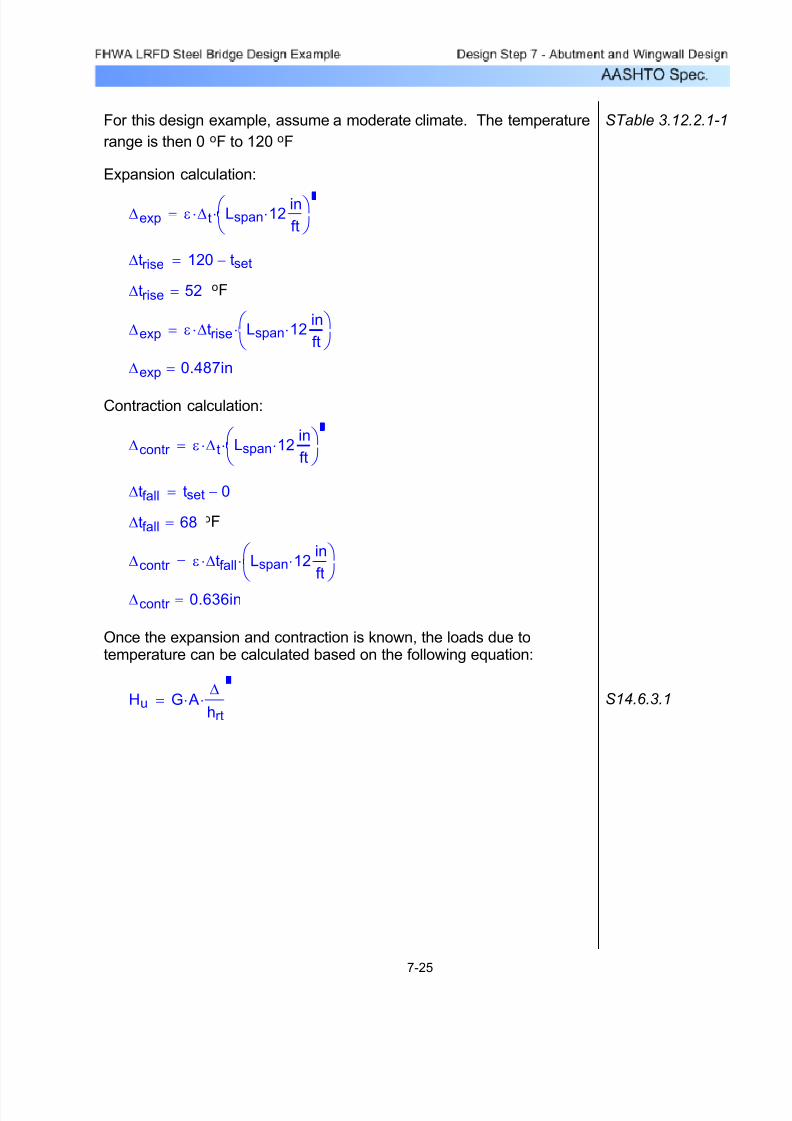
7/29/2019 LRFD steel design.pdf
http://slidepdf.com/reader/full/lrfd-steel-designpdf 368/646
S14.6.3.1Hu G A⋅∆
hrt⋅=
Once the expansion and contraction is known, the loads due totemperature can be calculated based on the following equation:
∆contr 0.636in=
∆contr ε ∆tfall⋅ Lspan 12⋅in
ft
⎛ ⎝
⎞ ⎠
⋅=
oF∆tfall 68=
∆tfall tset 0−=
∆contr ε ∆ t⋅ Lspan 12⋅in
ft
⎛ ⎝
⎞ ⎠
⋅=
Contraction calculation:
∆exp 0.487in=
∆exp ε ∆trise⋅ Lspan 12⋅in
ft
⎛ ⎝
⎞ ⎠
⋅=
oF∆trise 52=
∆trise 120 tset−=
∆exp ε ∆t⋅ Lspan 12⋅in
ft⎛ ⎝
⎞ ⎠
⋅=
Expansion calculation:
STable 3.12.2.1-1For this design example, assume a moderate climate. The temperature
range is then 0 oF to 120 oF
7-25

7/29/2019 LRFD steel design.pdf
http://slidepdf.com/reader/full/lrfd-steel-designpdf 369/646
Hufalltot 0.39K
ft=
HufalltotHufall 5⋅
Labut=
Now, multiply Hufall by five bearings and divide by the abutmentlength to get the total load due to temperature fall:
Hufall 3.63K=
Hufall G A⋅∆contr
hrt⋅=
Load due to temperature fall:
Hurisetot 0.30K
ft=
HurisetotHurise 5⋅
Labut=
Now, multiply Hurise by five bearings and divide by theabutment length to get the total load due to temperature rise:
per bearingHurise 2.77K=
Hurise G A⋅∆exp
hrt⋅=
Load due to temperature rise:
elastomer thickness (not including steel
reinforcement)
hrt 3.5in=
A 210.00in2=
area of the bearing pad in plan view A 14in 15⋅ in=
STable 14.7.5.2-1shear modulusG 0.095ksi=
Before the loads due to temperature rise and fall can be calculated, theneoprene bearing properties are needed (see Design Step 6). If thebearing pad design is not complete at the time the temperature loadsare being calculated, the temperature loads can be estimated by
assuming bearing pad properties that are larger than expected from thebearing pad design. The bearing pad properties for this designexample are:
7-26

7/29/2019 LRFD steel design.pdf
http://slidepdf.com/reader/full/lrfd-steel-designpdf 370/646
Design Step 7.7 - Analyze and Combine Force Effects
There are three critical locations where the force effects need tobe combined and analyzed for an abutment design. They are
the base or bottom of the backwall, the bottom of stem or top of footing, and the bottom of footing. For the backwall and stemdesign, transverse horizontal loads do not need to beconsidered due to the high moment of inertia about that axis, butat the bottom of footing, the transverse horizontal loads will needto be considered for the footing and pile design, although theyare still minimal.
Bottom of Abutment Backwall
In order to analyze and combine the force effects, the abutmentbackwall dimensions, the appropriate loads, and the application
location of the loads are needed. The small moment that iscreated by the top of the backwall corbel concrete will beneglected in this design example.
7 ' - 0
"
2 ' - 4 "
Horizontal earthload, R
EHbw
p
1'-8"
1'-3"9"
RLLbw
1'-2"
DLbw
CL Backwall
Live load surcharge,
RLSbw
Figure 7-8 Abutment Backwall Dimensions and Loading
The following limit states will be investigated for the backwallanalysis. The load factor for future wearing surface is given,but the load due to future wearing surface on the abutmentbackwall will be ignored since its effects are negligible. Also,limit states that are not shown either do not control or are notapplicable. In addition, Strength III and Strength V limit statesare included but generally will not control for an abutment withexpansion bearings. Strength III or Strength V may control for abutments supporting fixed bearings.
7-27
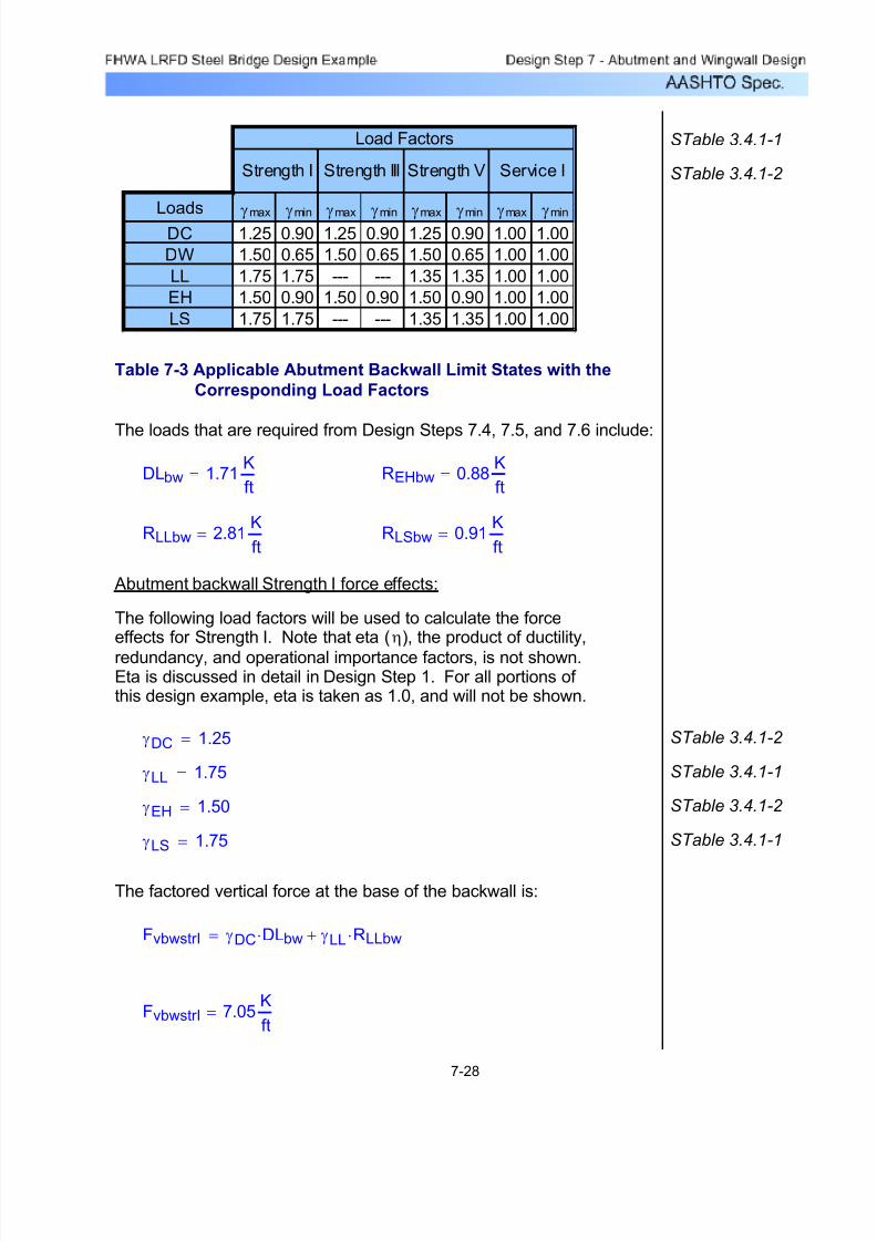
7/29/2019 LRFD steel design.pdf
http://slidepdf.com/reader/full/lrfd-steel-designpdf 371/646
FvbwstrI 7.05K
ft=
FvbwstrI γDC DLbw⋅ γLL RLLbw⋅+=
The factored vertical force at the base of the backwall is:
STable 3.4.1-1γLS 1.75=
STable 3.4.1-2 γEH 1.50=
STable 3.4.1-1γLL 1.75=
STable 3.4.1-2 γDC 1.25=
The following load factors will be used to calculate the forceeffects for Strength I. Note that eta (η), the product of ductility,
redundancy, and operational importance factors, is not shown.Eta is discussed in detail in Design Step 1. For all portions of this design example, eta is taken as 1.0, and will not be shown.
Abutment backwall Strength I force effects:
RLSbw 0.91K
ft=RLLbw 2.81
K
ft=
REHbw 0.88K
ft=DLbw 1.71
K
ft=
The loads that are required from Design Steps 7.4, 7.5, and 7.6 include:
Table 7-3 Applicable Abutment Backwall Limit States with the
Corresponding Load Factors
STable 3.4.1-2
STable 3.4.1-1
Loadsγmax γmin γmax γmin γmax γmin γmax γmin
DC 1.25 0.90 1.25 0.90 1.25 0.90 1.00 1.00
DW 1.50 0.65 1.50 0.65 1.50 0.65 1.00 1.00
LL 1.75 1.75 --- --- 1.35 1.35 1.00 1.00
EH 1.50 0.90 1.50 0.90 1.50 0.90 1.00 1.00
LS 1.75 1.75 --- --- 1.35 1.35 1.00 1.00
Load Factors
Strength I Strength III Strength V Service I
7-28
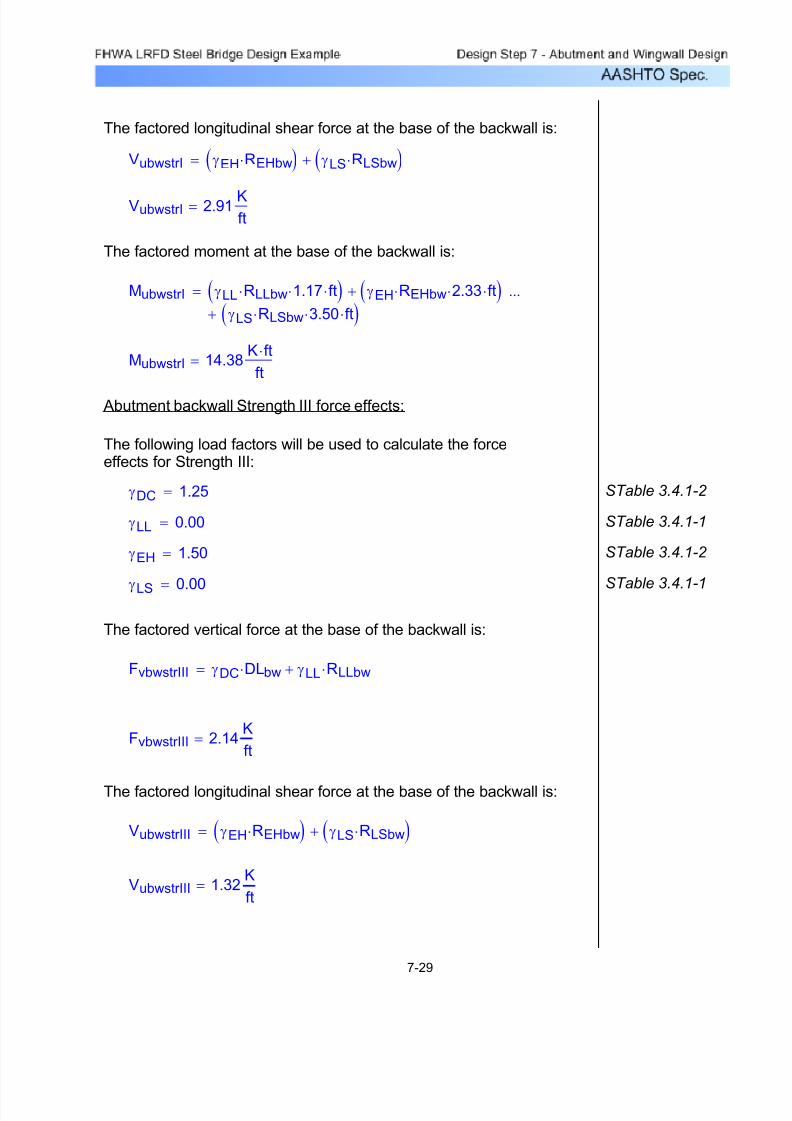
7/29/2019 LRFD steel design.pdf
http://slidepdf.com/reader/full/lrfd-steel-designpdf 372/646
VubwstrIII 1.32K
ft=
VubwstrIII γEH REHbw⋅( ) γLS RLSbw⋅( )+=
The factored longitudinal shear force at the base of the backwall is:
FvbwstrIII 2.14K
ft=
FvbwstrIII γDC DLbw⋅ γLL RLLbw⋅+=
The factored vertical force at the base of the backwall is:
STable 3.4.1-1γLS 0.00=
STable 3.4.1-2 γEH 1.50=
STable 3.4.1-1γLL 0.00=
STable 3.4.1-2 γDC 1.25=
The following load factors will be used to calculate the forceeffects for Strength III:
Abutment backwall Strength III force effects:
MubwstrI 14.38K ft⋅
ft=
MubwstrI γLL RLLbw⋅ 1.17⋅ ft⋅( ) γEH REHbw⋅ 2.33⋅ ft⋅( )+
γLS RLSbw⋅ 3.50⋅ ft⋅( )+
...=
The factored moment at the base of the backwall is:
VubwstrI 2.91 Kft
=
VubwstrI γEH REHbw⋅( ) γLS RLSbw⋅( )+=
The factored longitudinal shear force at the base of the backwall is:
7-29

7/29/2019 LRFD steel design.pdf
http://slidepdf.com/reader/full/lrfd-steel-designpdf 373/646
MubwstrV 11.80K ft⋅
ft=
MubwstrV γLL RLLbw⋅ 1.17⋅ ft⋅( ) γEH REHbw⋅ 2.33⋅ ft⋅( )+γLS RLSbw⋅ 3.50⋅ ft⋅( )+
...=
The factored moment at the base of the backwall is:
VubwstrV 2.55K
ft=
VubwstrV γEH REHbw⋅( ) γLS RLSbw⋅( )+=
The factored longitudinal shear force at the base of the backwall is:
FvbwstrV 5.93 Kft
=
FvbwstrV γDC DLbw⋅ γLL RLLbw⋅+=
The factored vertical force at the base of the backwall is:
STable 3.4.1-1γLS 1.35=
STable 3.4.1-2 γEH 1.50=
STable 3.4.1-1γLL 1.35=
STable 3.4.1-2 γDC 1.25=
The following load factors will be used to calculate the forceeffects for Strength V:
Abutment backwall Strength V force effects:
MubwstrIII 3.08K ft⋅
ft=
MubwstrIII γLL RLLbw⋅ 1.17⋅ ft⋅( ) γEH REHbw⋅ 2.33⋅ ft⋅( )+
γLS
RLSbw⋅ 3.50⋅ ft⋅
( )+
...=
The factored moment at the base of the backwall is:
7-30
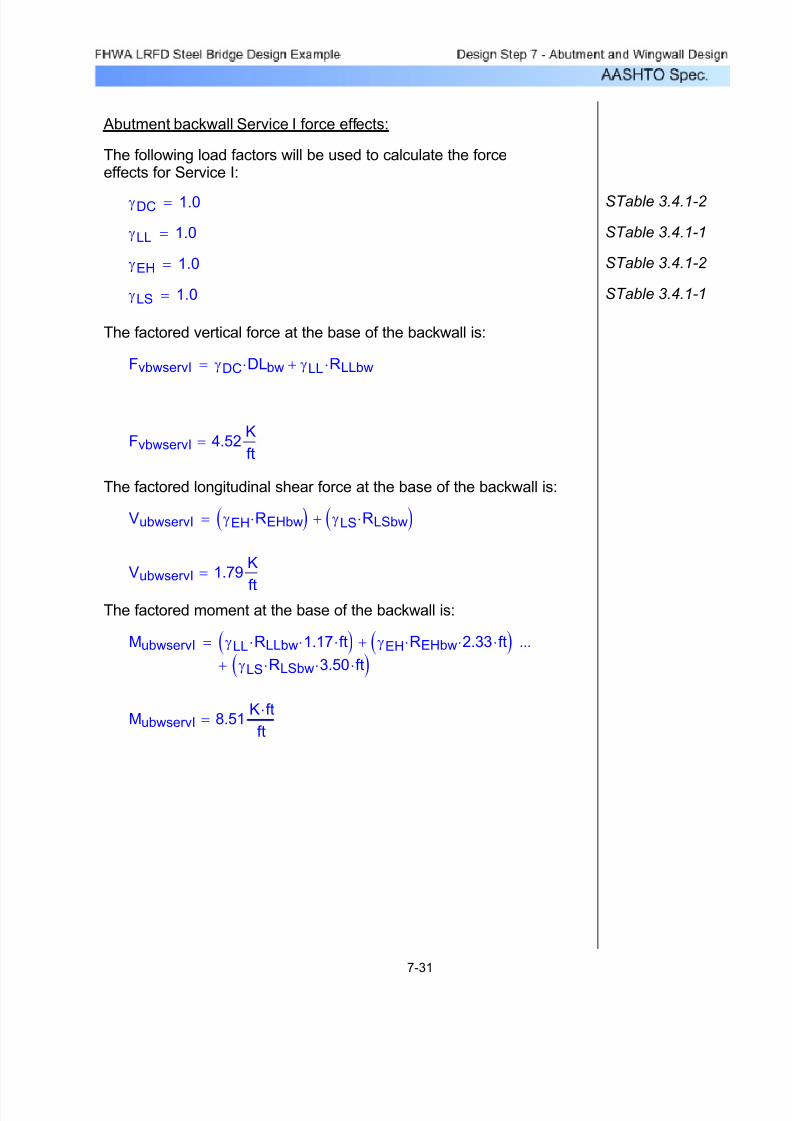
7/29/2019 LRFD steel design.pdf
http://slidepdf.com/reader/full/lrfd-steel-designpdf 374/646
MubwservI 8.51K ft⋅
ft=
MubwservI γLL RLLbw⋅ 1.17⋅ ft⋅( ) γEH REHbw⋅ 2.33⋅ ft⋅( )+
γLS RLSbw⋅ 3.50⋅ ft⋅( )+
...=
The factored moment at the base of the backwall is:
VubwservI 1.79K
ft
=
VubwservI γEH REHbw⋅( ) γLS RLSbw⋅( )+=
The factored longitudinal shear force at the base of the backwall is:
FvbwservI 4.52K
ft=
FvbwservI γDC DLbw⋅ γLL RLLbw⋅+=
The factored vertical force at the base of the backwall is:
STable 3.4.1-1γLS 1.0=
STable 3.4.1-2 γEH 1.0=
STable 3.4.1-1γLL 1.0=
STable 3.4.1-2 γDC 1.0=
The following load factors will be used to calculate the forceeffects for Service I:
Abutment backwall Service I force effects:
7-31

7/29/2019 LRFD steel design.pdf
http://slidepdf.com/reader/full/lrfd-steel-designpdf 375/646
The maximum factored backwall vertical force, shear force, andmoment for the strength limit state are:
Fvbwmax max FvbwstrI FvbwstrIII, FvbwstrV,( )=
Fvbwmax 7.05K
ft=
Vubwmax max VubwstrI VubwstrIII, VubwstrV,( )=
Vubwmax 2.91K
ft=
Mubwmax max MubwstrI MubwstrIII, MubwstrV,( )=
Mubwmax 14.38K ft⋅
ft=
7-32

7/29/2019 LRFD steel design.pdf
http://slidepdf.com/reader/full/lrfd-steel-designpdf 376/646
Bottom of Abutment Stem
The combination of force effects for the bottom of abutmentstem are similar to the backwall with the addition of thesuperstructure dead and live loads.
Figure 7-9 Abutment Stem Dimensions and Loading
The force effects for the stem will be combined for the same limitstates as the backwall. The loads and load factors are also similar to the backwall with the addition of wind on structure, wind on liveload, and thermal effects. As with the backwall, the extreme eventlimit states will not be investigated.
7-33
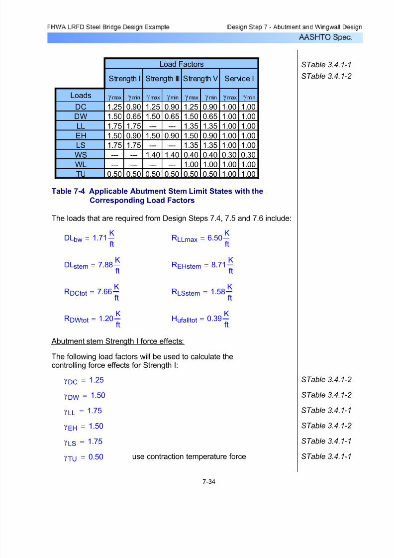
7/29/2019 LRFD steel design.pdf
http://slidepdf.com/reader/full/lrfd-steel-designpdf 377/646
STable 3.4.1-1use contraction temperature forceγTU 0.50=
STable 3.4.1-1γLS 1.75=
STable 3.4.1-2 γEH 1.50=
STable 3.4.1-1γLL 1.75=
STable 3.4.1-2 γDW 1.50=
STable 3.4.1-2 γDC 1.25=
The following load factors will be used to calculate thecontrolling force effects for Strength I:
Abutment stem Strength I force effects:
Hufalltot 0.39K
ft=RDWtot 1.20
K
ft=
RLSstem 1.58
K
ft=RDCtot 7.66
K
ft=
REHstem 8.71K
ft=DLstem 7.88
K
ft=
RLLmax 6.50K
ft=DLbw 1.71
K
ft=
The loads that are required from Design Steps 7.4, 7.5 and 7.6 include:
Table 7-4 Applicable Abutment Stem Limit States with the
Corresponding Load Factors
STable 3.4.1-2
STable 3.4.1-1
Loads γmax γmin γmax γmin γmax γmin γmax γmin
DC 1.25 0.90 1.25 0.90 1.25 0.90 1.00 1.00
DW 1.50 0.65 1.50 0.65 1.50 0.65 1.00 1.00
LL 1.75 1.75 --- --- 1.35 1.35 1.00 1.00
EH 1.50 0.90 1.50 0.90 1.50 0.90 1.00 1.00
LS 1.75 1.75 --- --- 1.35 1.35 1.00 1.00
WS --- --- 1.40 1.40 0.40 0.40 0.30 0.30
WL --- --- --- --- 1.00 1.00 1.00 1.00
TU 0.50 0.50 0.50 0.50 0.50 0.50 1.00 1.00
Load Factors
Strength I Strength III Strength V Service I
7-34
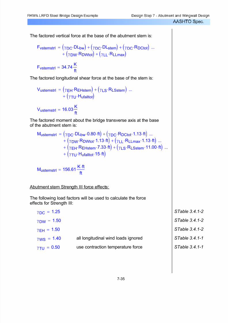
7/29/2019 LRFD steel design.pdf
http://slidepdf.com/reader/full/lrfd-steel-designpdf 378/646
STable 3.4.1-1use contraction temperature forceγTU 0.50=
STable 3.4.1-1all longitudinal wind loads ignoredγWS 1.40=
STable 3.4.1-2 γEH 1.50=
STable 3.4.1-2 γDW 1.50=
STable 3.4.1-2 γDC 1.25=
The following load factors will be used to calculate the forceeffects for Strength III:
Abutment stem Strength III force effects:
MustemstrI 156.61K ft⋅ft=
MustemstrI γDC DLbw⋅ 0.80⋅ ft⋅( ) γDC RDCtot⋅ 1.13⋅ ft⋅( )+
γDW RDWtot⋅ 1.13⋅ ft⋅( ) γLL RLLmax⋅ 1.13⋅ ft⋅( )++
...
γEH REHstem⋅ 7.33⋅ ft⋅( ) γLS RLSstem⋅ 11.00⋅ ft⋅( )++
...
γTU Hufalltot⋅ 15⋅ ft⋅( )+
...
=
The factored moment about the bridge transverse axis at the baseof the abutment stem is:
VustemstrI 16.03K
ft
=
VustemstrI γEH REHstem⋅( ) γLS RLSstem⋅( )+
γTU Hufalltot⋅( )+
...=
The factored longitudinal shear force at the base of the stem is:
FvstemstrI 34.74K
ft=
FvstemstrI γDC DLbw⋅( ) γDC DLstem⋅( )+ γDC RDCtot⋅( )+
γDW
RDWtot
⋅
( )γ
LLR
LLmax⋅
( )++
...=
The factored vertical force at the base of the abutment stem is:
7-35

7/29/2019 LRFD steel design.pdf
http://slidepdf.com/reader/full/lrfd-steel-designpdf 379/646
STable 3.4.1-1use contraction temperature forceγTU 0.50=
STable 3.4.1-1only applicable for wind angle of 0 degreesγWL 1.00=
STable 3.4.1-1all longitudinal wind loads ignoredγWS 0.40=
STable 3.4.1-1γLS 1.35=STable 3.4.1-2 γEH 1.50=
STable 3.4.1-1γLL 1.35=
STable 3.4.1-2 γDW 1.50=
STable 3.4.1-2 γDC 1.25=
The following load factors will be used to calculate the forceeffects for Strength V:
Abutment stem Strength V force effects:
MustemstrIII 113.25K ft⋅ft
=
MustemstrIII γDC DLbw⋅ 0.80⋅ ft⋅( ) γDC RDCtot⋅ 1.13⋅ ft⋅( )+
γDW RDWtot⋅ 1.13⋅ ft⋅( ) γEH REHstem⋅ 7.33⋅ ft⋅( )++
...
γTU Hufalltot⋅ 15⋅ ft⋅( )+
...
=
The factored moment about the bridge transverse axis at the baseof the abutment stem is:
VustemstrIII 13.26K
ft=
VustemstrIII γEH REHstem⋅( ) γTU Hufalltot⋅( )+=
The factored longitudinal shear force at the base of the stem is:
FvstemstrIII 23.36K
ft=
FvstemstrIII γDC DLbw⋅( ) γDC DLstem⋅( )+
γDC RDCtot⋅( ) γDW RDWtot⋅( )++
...=
The factored vertical force at the base of the abutment stem is:
7-36

7/29/2019 LRFD steel design.pdf
http://slidepdf.com/reader/full/lrfd-steel-designpdf 380/646
The factored vertical force at the base of the abutment stem is:
FvstemstrV γDC DLbw⋅( ) γDC DLstem⋅( )+
γDC RDCtot⋅( ) γDW RDWtot⋅( )++
...
γLL RLLmax⋅( )+
...
=
FvstemstrV 32.14K
ft=
The factored longitudinal shear force at the base of the stem is:
VustemstrV γEH REHstem⋅( ) γLS RLSstem⋅( )+
γTU Hufalltot⋅( )+
...=
VustemstrV 15.40K
ft=
The factored moment about the bridge transverse axis at the baseof the abutment stem is:
MustemstrV γDC DLbw⋅ 0.80⋅ ft⋅( ) γDC RDCtot⋅ 1.13⋅ ft⋅( )+
γDW RDWtot⋅ 1.13⋅ ft⋅( ) γLL RLLmax⋅ 1.13⋅ ft⋅( )++
...
γEH REHstem⋅ 7.33⋅ ft⋅( ) γLS RLSstem⋅ 11.00⋅ ft⋅( )++
...
γTU Hufalltot⋅ 15⋅ ft⋅( )+
...
=
MustemstrV 146.70K ft⋅ft
=
7-37
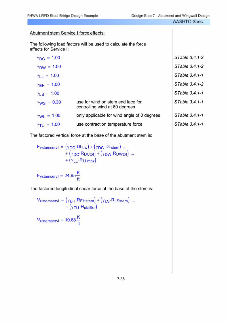
7/29/2019 LRFD steel design.pdf
http://slidepdf.com/reader/full/lrfd-steel-designpdf 381/646
VustemservI 10.68K
ft=
VustemservI γEH REHstem⋅( ) γLS RLSstem⋅( )+
γTU Hufalltot⋅( )+
...=
The factored longitudinal shear force at the base of the stem is:
FvstemservI 24.95K
ft=
FvstemservI γDC DLbw⋅( ) γDC DLstem⋅( )+
γDC RDCtot⋅( ) γDW RDWtot⋅( )++
...
γLL RLLmax⋅( )+
...
=
The factored vertical force at the base of the abutment stem is:
STable 3.4.1-1use contraction temperature forceγTU 1.00=
STable 3.4.1-1only applicable for wind angle of 0 degreesγWL 1.00=
STable 3.4.1-1use for wind on stem end face for controlling wind at 60 degrees
γWS 0.30=
STable 3.4.1-1γLS 1.00=
STable 3.4.1-2 γEH 1.00=
STable 3.4.1-1γLL 1.00=
STable 3.4.1-2 γDW 1.00=
STable 3.4.1-2 γDC 1.00=
The following load factors will be used to calculate the forceeffects for Service I:
Abutment stem Service I force effects:
7-38

7/29/2019 LRFD steel design.pdf
http://slidepdf.com/reader/full/lrfd-steel-designpdf 382/646
The factored moment about the bridge transverse axis atthe base of the abutment stem is:
MustemservI γDC DLbw⋅ 0.80⋅ ft⋅( ) γDC RDCtot⋅ 1.13⋅ ft⋅( )+
γDW RDWtot⋅ 1.13⋅ ft⋅( ) γLL RLLmax⋅ 1.13⋅ ft⋅( )++
...
γEH REHstem⋅ 7.33⋅ ft⋅( ) γLS RLSstem⋅ 11.00⋅ ft⋅( )++...
γTU Hufalltot⋅ 15⋅ ft⋅( )+
...
=
MustemservI 105.82K ft⋅ft
=
The maximum factored abutment stem vertical force, shear force,and moment for the strength limit state are:
Fvstemmax max FvstemstrI FvstemstrIII, FvstemstrV,( )=
Fvstemmax 34.74K
ft=
Vustemmax
max VustemstrI
VustemstrIII
, VustemstrV
,( )
=
Vustemmax 16.03K
ft=
Mustemmax max MustemstrI MustemstrIII, MustemstrV,( )=
Mustemmax 156.61K ft⋅ft
=
7-39

7/29/2019 LRFD steel design.pdf
http://slidepdf.com/reader/full/lrfd-steel-designpdf 383/646
Bottom of Abutment Footing
The combination of force effects for the bottom of abutmentfooting are similar to the backwall and stem with the additionof the earth load on the abutment heel. Also, dynamic load
allowance must be removed from the live load portion of theforce effects for foundation components that are completelybelow the ground level.
S3.6.2.1
Figure 7-10 Abutment Footing Dimensions and Loading
7-40

7/29/2019 LRFD steel design.pdf
http://slidepdf.com/reader/full/lrfd-steel-designpdf 384/646
WSsublongend60 2.67K=RLLmax1 5.34K
ft=
WSsubtransend60 1.54K=RLLmin1 0.68−K
ft=
WLtrans0 6.00K=RDWtot 1.20K
ft=
WSsubtransend0 3.08K=RDCtot 7.66K
ft
=
WSsupertrans0 30.69K=DLearth 10.56K
ft=
Hufalltot 0.39K
ft=DLftg 3.84
K
ft=
RLSftg 1.76 Kft
=DLstem 7.88 Kft
=
REHftg 10.80K
ft=DLbw 1.71
K
ft=
The loads that are required from Design Steps 7.4, 7.5, and 7.6 include:
Table 7-5 Applicable Abutment Footing Limit States with the
Corresponding Load Factors
STable 3.4.1-2
STable 3.4.1-1
Loads γmax γmin γmax γmin γmax γmin γmax γmin
DC 1.25 0.90 1.25 0.90 1.25 0.90 1.00 1.00
DW 1.50 0.65 1.50 0.65 1.50 0.65 1.00 1.00
LL 1.75 1.75 --- --- 1.35 1.35 1.00 1.00
EH 1.50 0.90 1.50 0.90 1.50 0.90 1.00 1.00
EV 1.35 1.00 1.35 1.00 1.35 1.00 1.00 1.00
LS 1.75 1.75 --- --- 1.35 1.35 1.00 1.00
WS --- --- 1.40 1.40 0.40 0.40 0.30 0.30WL --- --- --- --- 1.00 1.00 1.00 1.00
TU 0.50 0.50 0.50 0.50 0.50 0.50 1.00 1.00
Load FactorsStrength I Strength III Strength V Service I
The force effects for the bottom of footing will be combined for thesame limit states as the backwall and stem. The loads and loadfactors are also similar with the addition of vertical earth load.
7-41

7/29/2019 LRFD steel design.pdf
http://slidepdf.com/reader/full/lrfd-steel-designpdf 385/646
The load factors for the loads thatproduce transverse horizontal forcesare zero for Strength I.
FtraftgstrI 0K
ft=
The factored transverse horizontal force at the bottom of footing is:
FlonftgstrI 19.49K
ft=
FlonftgstrI γEH REHftg⋅( ) γLS RLSftg⋅( )+
γTU Hufalltot⋅( )+
...⎡
⎣
⎤
⎦
=
The factored longitudinal horizontal force at the bottom of footing is:
FvftgstrI 51.76K
ft=
FvftgstrI γDC DLbw⋅( ) γDC DLstem⋅( )+
γDC DLftg⋅( ) γEV DLearth⋅( )++
...
γDC RDCtot⋅( ) γDW RDWtot⋅( )++
...
γLL
RLLmax1⋅
( )+
...
=
The factored vertical force at the bottom of footing is:
STable 3.4.1-1use contraction temperature forceγTU 0.50=
STable 3.4.1-1γLS 1.75=
STable 3.4.1-2 use maximum value to maximizethe pile loads
γEV 1.35=
STable 3.4.1-2 γEH 1.50=
STable 3.4.1-1γLL 1.75=
STable 3.4.1-2 γDW 1.50=
STable 3.4.1-2 γDC 1.25=
The following load factors will be used to calculate the
controlling force effects for Strength I:
Abutment bottom of footing Strength I force effects using themaximum load factors:
7-42
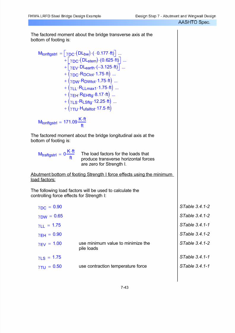
7/29/2019 LRFD steel design.pdf
http://slidepdf.com/reader/full/lrfd-steel-designpdf 386/646
STable 3.4.1-1use contraction temperature forceγTU 0.50=
STable 3.4.1-1γLS 1.75=
STable 3.4.1-2 use minimum value to minimize thepile loads
γEV 1.00=
STable 3.4.1-2 γEH 0.90=
STable 3.4.1-1γLL 1.75=
STable 3.4.1-2 γDW 0.65=
STable 3.4.1-2 γDC 0.90=
The following load factors will be used to calculate thecontrolling force effects for Strength I:
Abutment bottom of footing Strength I force effects using the minimumload factors:
The load factors for the loads thatproduce transverse horizontal forcesare zero for Strength I.
MtraftgstrI 0K ft⋅ft
=
The factored moment about the bridge longitudinal axis at thebottom of footing is:
MlonftgstrI 171.09K ft⋅ft
=
MlonftgstrI γDC DLbw( )⋅ 0.177− ft⋅( )⋅
γDC DLstem( )⋅ 0.625 ft⋅( )⋅+
...
γEV DLearth⋅ 3.125− ft⋅( )⋅+...
γDC RDCtot⋅ 1.75⋅ ft⋅( )+
...
γDW RDWtot⋅ 1.75⋅ ft⋅( )+
...
γLL RLLmax1⋅ 1.75⋅ ft⋅( )+
...
γEH REHftg⋅ 8.17⋅ ft⋅( )+
...
γLS RLSftg⋅ 12.25⋅ ft⋅( )+
...
γTU Hufalltot⋅ 17.5⋅ ft⋅( )+
...
=
The factored moment about the bridge transverse axis at thebottom of footing is:
7-43

7/29/2019 LRFD steel design.pdf
http://slidepdf.com/reader/full/lrfd-steel-designpdf 387/646
The factored vertical force at the bottom of footing is:
FvftgstrImin γDC DLbw⋅( ) γDC DLstem⋅( )+
γDC DLftg⋅( ) γEV DLearth⋅( )++
...
γDC RDCtot⋅( ) γDW RDWtot⋅( )++ ...
γLL RLLmin1⋅( )+
...
=
FvftgstrImin 29.14K
ft=
The factored longitudinal horizontal force at the bottom of footing is:
FlonftgstrImin γEH REHftg⋅( ) γLS RLSftg⋅( )+
γTU Hufalltot⋅( )+
...=
FlonftgstrImin 13.00K
ft=
The factored transverse horizontal force at the bottom of footing is:
FtraftgstrImin 0K
ft= The load factors for the loads that
produce transverse horizontal forces
are zero for Strength I.
The factored moment about the bridge transverse axis at thebottom of footing is:
MlonftgstrImin γDC DLbw( )⋅ 0.177− ft⋅( )⋅
γDC DLstem( )⋅ 0.625 ft⋅( )⋅+
...
γEV DLearth⋅ 3.125− ft⋅( )⋅+
...
γDC RDCtot⋅ 1.75⋅ ft⋅( )+
...
γDW RDWtot⋅ 1.75⋅ ft⋅( )+
...
γLL RLLmin1⋅ 1.75⋅ ft⋅( )+
...
γEH REHftg⋅ 8.17⋅ ft⋅( )+...
γLS RLSftg⋅ 12.25⋅ ft⋅( )+
...
γTU Hufalltot⋅ 17.5⋅ ft⋅( )+
...
=
MlonftgstrImin 103.16K ft⋅ft
=
7-44

7/29/2019 LRFD steel design.pdf
http://slidepdf.com/reader/full/lrfd-steel-designpdf 388/646
Vertical wind load will be ignored since the moment of inertia aboutthe abutment longitudinal axis is so large.
STable 3.4.1-1use contraction temperature forceγTU 0.50=
STable 3.4.1-1use a wind angle of 0 degreesγWS 1.40=
STable 3.4.1-2 use minimum value to maximizethe longitudinal moment
γEV 1.00=
STable 3.4.1-2 γEH 1.50=
STable 3.4.1-2 γDW 1.50=
STable 3.4.1-2 γDC 1.25=
The following load factors will be used to calculate the force
effects for Strength III:
S3.4.1Load Combinations
There are numerous load factor combinations for each
limit state as can be seen from STables 3.4.1-1 and
3.4.1-2 . It is possible to check one limit state, such as
Strength I, over and over again using many differentload factor combinations to obtain the controllingfactored effects. The engineer should use engineering
judgement when selecting the most appropriate loadfactor for each individual load within a limit state.
For the Strength III force effects below, the horizontalearth load is factored by the maximum load factor while the vertical earth load is factored by the minimumfactor to maximize the overturning moment.
Abutment bottom of footing Strength III force effects:
The load factors for the loads that
produce transverse horizontal forcesare zero for Strength I.
MtraftgstrImin 0K
ft
=
The factored moment about the bridge longitudinal axis at thebottom of footing is:
7-45
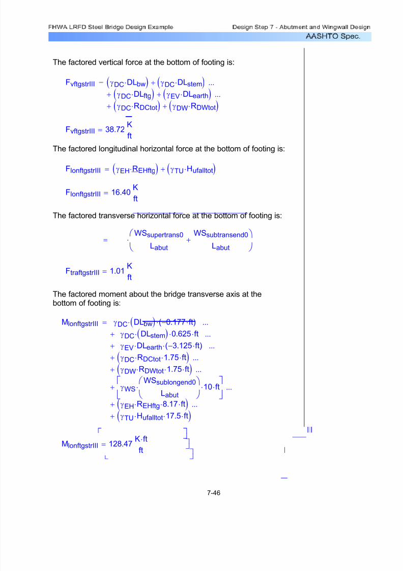
7/29/2019 LRFD steel design.pdf
http://slidepdf.com/reader/full/lrfd-steel-designpdf 389/646
The factored vertical force at the bottom of footing is:
FvftgstrIII γDC DLbw⋅( ) γDC DLstem⋅( )+
γDC
DLftg⋅
( )γ
EV
DLearth⋅
( )++
...
γDC RDCtot⋅( ) γDW RDWtot⋅( )++
...
=
FvftgstrIII 38.72K
ft=
The factored longitudinal horizontal force at the bottom of footing is:
FlonftgstrIII γEH REHftg⋅( ) γTU Hufalltot⋅( )+=
FlonftgstrIII 16.40K
ft
=
The factored transverse horizontal force at the bottom of footing is:
FtraftgstrIII γWS
WSsupertrans0
Labut
WSsubtransend0
Labut+
⎛
⎝
⎞
⎠⋅=
FtraftgstrIII 1.01K
ft=
The factored moment about the bridge transverse axis at thebottom of footing is:
MlonftgstrIII γDC DLbw( )⋅ 0.177− ft⋅( )⋅
γDC DLstem( )⋅ 0.625⋅ ft⋅+
...
γEV DLearth⋅ 3.125− ft⋅( )⋅+
...
γDC RDCtot⋅ 1.75⋅ ft⋅( )+
...
γDW RDWtot⋅ 1.75⋅ ft⋅( )+
...
γWS
WSsublongend0
Labut
⎛
⎝
⎞
⎠
⋅ 10⋅ ft⋅⎡
⎣
⎤
⎦
+
...
γEH REHftg⋅ 8.17⋅ ft⋅( )+
...
γTU Hufalltot⋅ 17.5⋅ ft⋅( )+...
=
MlonftgstrIII 128.47K ft⋅ft
=
7-46
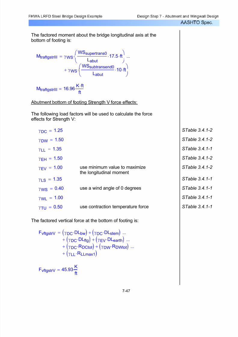
7/29/2019 LRFD steel design.pdf
http://slidepdf.com/reader/full/lrfd-steel-designpdf 390/646
FvftgstrV 45.93K
ft=
FvftgstrV γDC DLbw⋅( ) γDC DLstem⋅( )+
γDC DLftg⋅( ) γEV DLearth⋅( )++
...
γDC RDCtot⋅( ) γDW RDWtot⋅( )++
...
γLL RLLmax1⋅( )+
...
=
The factored vertical force at the bottom of footing is:
STable 3.4.1-1use contraction temperature forceγTU 0.50=
STable 3.4.1-1γWL 1.00=
STable 3.4.1-1use a wind angle of 0 degreesγWS 0.40=
STable 3.4.1-1γLS 1.35=
STable 3.4.1-2 use minimum value to maximizethe longitudinal moment
γEV 1.00=
STable 3.4.1-2 γEH 1.50=
STable 3.4.1-1γLL 1.35=
STable 3.4.1-2 γDW 1.50=
STable 3.4.1-2 γDC 1.25=
The following load factors will be used to calculate the force
effects for Strength V:
Abutment bottom of footing Strength V force effects:
MtraftgstrIII 16.96K ft⋅ft
=
MtraftgstrIII
γWS
WSsupertrans0
Labut17.5⋅ ft⋅
⎛
⎝
⎞
⎠⋅
γWS
WSsubtransend0
Labut10⋅ ft⋅
⎛
⎝
⎞
⎠⋅+
...=
The factored moment about the bridge longitudinal axis at thebottom of footing is:
7-47
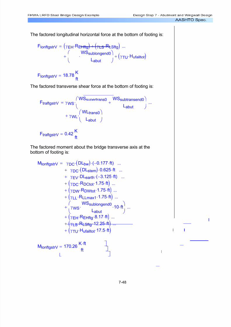
7/29/2019 LRFD steel design.pdf
http://slidepdf.com/reader/full/lrfd-steel-designpdf 391/646
The factored longitudinal horizontal force at the bottom of footing is:
FlonftgstrV γEH REHftg⋅( ) γLS RLSftg⋅( )+
γWS
WSsublongend0
Labut⋅
⎛
⎝
⎞
⎠ γTU Hufalltot⋅( )++
...=
FlonftgstrV 18.78K
ft=
The factored transverse shear force at the bottom of footing is:
FtraftgstrV γWS
WSsupertrans0
Labut
WSsubtransend0
Labut+
⎛
⎝
⎞
⎠⋅
γWL
WLtrans0
Labut⎛ ⎝ ⎞ ⎠
⋅+
...=
FtraftgstrV 0.42K
ft=
The factored moment about the bridge transverse axis at thebottom of footing is:
MlonftgstrV γDC DLbw( )⋅ 0.177− ft⋅( )⋅
γDC DLstem( )⋅ 0.625⋅ ft⋅+
...
γEV DLearth⋅ 3.125− ft⋅( )⋅+ ...
γDC RDCtot⋅ 1.75⋅ ft⋅( )+
...
γDW RDWtot⋅ 1.75⋅ ft⋅( )+
...
γLL RLLmax1⋅ 1.75⋅ ft⋅( )+
...
γWS
WSsublongend0
Labut⋅ 10⋅ ft⋅
⎛
⎝
⎞
⎠+
...
γEH REHftg⋅ 8.17⋅ ft⋅( )+
...
γLS RLSftg⋅ 12.25⋅ ft⋅( )+
...
γTU Hufalltot⋅ 17.5⋅ ft⋅( )+
...
=
MlonftgstrV 170.26K ft⋅ft
=
7-48

7/29/2019 LRFD steel design.pdf
http://slidepdf.com/reader/full/lrfd-steel-designpdf 392/646
FvftgservI 38.19K
ft=
FvftgservI γDC DLbw⋅( ) γDC DLstem⋅( )+
γDC DLftg⋅( ) γEV DLearth⋅( )++
...
γDC RDCtot⋅( ) γDW RDWtot⋅( )++
...
γLL RLLmax1⋅( )+
...
=
The factored vertical force at the bottom of footing is:
STable 3.4.1-1use contraction temperature forceγTU 1.00=
STable 3.4.1-1γWL 1.00=
STable 3.4.1-1use wind at 0 degreesγWS 0.30=
STable 3.4.1-1γLS 1.00=
STable 3.4.1-2 γEV 1.00=
STable 3.4.1-2 γEH 1.00=
STable 3.4.1-1γLL 1.00=
STable 3.4.1-2 γDW 1.00=
STable 3.4.1-2 γDC 1.00=
The following load factors will be used to calculate the forceeffects for Service I:
Abutment bottom of footing Service I force effects for wind at 0degrees and maximum live load:
MtraftgstrV 8.75K ft⋅ft
=
MtraftgstrV γWS
WSsupertrans0
Labut
17.5⋅ ft⋅⎛
⎝
⎞
⎠⋅
γWS
WSsubtransend0
Labut10⋅ ft⋅
⎛
⎝
⎞
⎠⋅+
...
γWL
WLtrans0
Labut30.5⋅ ft
⎛
⎝
⎞
⎠⋅+
...
=
The factored moment about the bridge longitudinal axis at thebottom of footing is:
7-49

7/29/2019 LRFD steel design.pdf
http://slidepdf.com/reader/full/lrfd-steel-designpdf 393/646
The factored longitudinal shear force at the bottom of footing is:
FlonftgservI γEH REHftg⋅( ) γLS RLSftg⋅( )+
γWS
WSsublongend0
Labut⋅⎛
⎝
⎞
⎠+
...
γTU Hufalltot⋅( )+
...
=
FlonftgservI 12.96K
ft=
The factored transverse shear force at the bottom of footing is:
FtraftgservI γWS
WSsupertrans0
Labut
⎛
⎝
⎞
⎠
⋅
γWS
WSsubtransend0
Labut
⎛
⎝
⎞
⎠⋅+
...
γWL
WLtrans0
Labut
⎛
⎝
⎞
⎠⋅+
...
=
FtraftgservI 0.34K
ft=
The factored moment about the bridge transverse axis at thebottom of footing is:
MlonftgservI γDC DLbw( )⋅ 0.177− ft⋅( )⋅
γDC DLstem( )⋅ 0.625⋅ ft⋅+
...
γEV DLearth⋅ 3.125− ft⋅( )⋅+
...
γDC RDCtot⋅ 1.75⋅ ft⋅( )+
...
γDW RDWtot⋅ 1.75⋅ ft⋅( )+
...
γLL RLLmax1⋅ 1.75⋅ ft⋅( )+
...
γWS
WSsublongend0
Labut
⋅ 10⋅ ft⋅⎛
⎝
⎞
⎠
+
...
γEH REHftg⋅ 8.17⋅ ft⋅( )+
...
γLS RLSftg⋅ 12.25⋅ ft⋅( )+
...
γTU Hufalltot⋅ 17.5⋅ ft⋅( )+
...
=
MlonftgservI 113.12K ft⋅ft
=
7-50
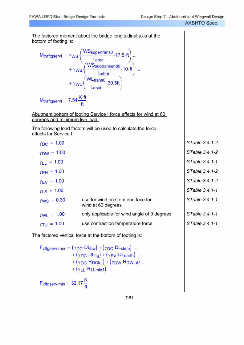
7/29/2019 LRFD steel design.pdf
http://slidepdf.com/reader/full/lrfd-steel-designpdf 394/646
FvftgservImin 32.17K
ft=
FvftgservImin γDC DLbw⋅( ) γDC DLstem⋅( )+
γDC DLftg⋅( ) γEV DLearth⋅( )++
...
γDC RDCtot⋅( ) γDW RDWtot⋅( )++
...
γLL RLLmin1⋅( )+
...
=
The factored vertical force at the bottom of footing is:
STable 3.4.1-1use contraction temperature forceγTU 1.00=
STable 3.4.1-1only applicable for wind angle of 0 degreesγWL 1.00=
STable 3.4.1-1use for wind on stem end face for wind at 60 degrees
γWS 0.30=
STable 3.4.1-1γLS 1.00=
STable 3.4.1-2 γEV 1.00=
STable 3.4.1-2 γEH 1.00=
STable 3.4.1-1γLL 1.00=
STable 3.4.1-2 γDW 1.00=
STable 3.4.1-2 γDC 1.00=
The following load factors will be used to calculate the forceeffects for Service I:
Abutment bottom of footing Service I force effects for wind at 60
degrees and minimum live load:
MtraftgservI 7.54K ft⋅ft
=
MtraftgservI γWS
WSsupertrans0
Labut
17.5⋅ ft⋅⎛
⎝
⎞
⎠
⋅
γWS
WSsubtransend0
Labut10⋅ ft⋅
⎛
⎝
⎞
⎠⋅+
...
γWL
WLtrans0
Labut30.5⋅ ft
⎛
⎝
⎞
⎠⋅+
...
=
The factored moment about the bridge longitudinal axis at thebottom of footing is:
7-51
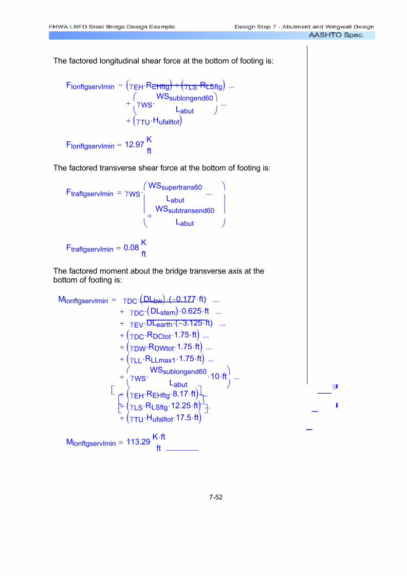
7/29/2019 LRFD steel design.pdf
http://slidepdf.com/reader/full/lrfd-steel-designpdf 395/646
The factored longitudinal shear force at the bottom of footing is:
FlonftgservImin γEH REHftg⋅( ) γLS RLSftg⋅( )+
γWS
WSsublongend60
Labut⋅⎛ ⎝ ⎞ ⎠
+
...
γTU Hufalltot⋅( )+
...
=
FlonftgservImin 12.97K
ft=
The factored transverse shear force at the bottom of footing is:
FtraftgservImin γWS
WSsupertrans60
LabutWSsubtransend60
Labut+
...⎛
⎜⎜
⎝
⎞
⎟⎟
⎠
⋅=
FtraftgservImin 0.08K
ft=
The factored moment about the bridge transverse axis at thebottom of footing is:
MlonftgservImin γDC DLbw( )⋅ 0.177− ft⋅( )⋅γDC DLstem( )⋅ 0.625⋅ ft⋅+ ...
γEV DLearth⋅ 3.125− ft⋅( )⋅+
...
γDC RDCtot⋅ 1.75⋅ ft⋅( )+
...
γDW RDWtot⋅ 1.75⋅ ft⋅( )+
...
γLL RLLmax1⋅ 1.75⋅ ft⋅( )+
...
γWS
WSsublongend60
Labut⋅ 10⋅ ft⋅
⎛
⎝
⎞
⎠+
...
γEH REHftg⋅ 8.17⋅ ft⋅( )+
...
γLS RLSftg⋅ 12.25⋅ ft⋅( )+
...
γTU Hufalltot⋅ 17.5⋅ ft⋅( )+...
=
MlonftgservImin 113.29K ft⋅ft
=
7-52

7/29/2019 LRFD steel design.pdf
http://slidepdf.com/reader/full/lrfd-steel-designpdf 396/646
The factored moment about the bridge longitudinal axis at thebottom of footing is:
MtraftgservImin γWS
WSsupertrans60
Labut17.5⋅ ft⋅
⎛
⎝
⎞
⎠⋅
γWSWSsublongend60
Labut10⋅ ft⋅⎛
⎝ ⎞ ⎠
⋅+
...=
MtraftgservImin 1.34K ft⋅ft
=
The following table summarizes the combined forces at the bottom of footing that were calculated above. The forces were calculated at thecenter of the bottom of footing. The values shown in the table weremultiplied by the abutment length to obtain the total effect. These forcesare required for the geotechnical engineer to design the pile foundation.
It should be noted that Design Step P was based on preliminary pilefoundation design forces. In an actual design, the geotechnicalengineer would need to revisit the pile foundation design calculationsand update the results based on the final design bottom of footingforces given below.
Limit State
Vertical
Force
(K)
Long.
Moment
(K-ft)
Trans.
Moment
(K-ft)
Lateral
Load
(Long.
Direction)
(K)
Lateral
Load
(Trans.
Direction)
(K)
Strength IMax/Final
2426 8020 0 913 0
Strength I
Min/Final1366 4836 0 610 0
Strength III
Max/Final1815 6022 795 769 47
Service I
Max/Final1790 5302 353 607 16
Service I
Min/Final1508 5310 63 608 4
Table 7-6 Pile Foundation Design Forces
7-53
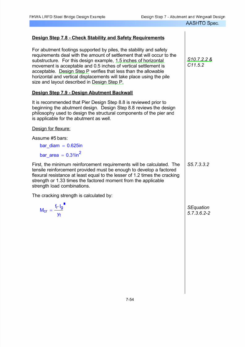
7/29/2019 LRFD steel design.pdf
http://slidepdf.com/reader/full/lrfd-steel-designpdf 397/646

7/29/2019 LRFD steel design.pdf
http://slidepdf.com/reader/full/lrfd-steel-designpdf 398/646
Centroidal
Axis
Front face of backwall at base
#5 bars@ 8.0 in
spacing
1 ' - 8 "
2
1 3 / 1 6 "
1 0 "
1'-0"
Figure 7-11 Abutment Backwall Cracking Moment Dimensions
f r 0.24 f'c⋅= S5.4.2.6
f r 0.48ksi=
Ig 112
12in( ) 20in( )3=
Ig 8000in4
=
yt 10in=
Mcr
f r Ig⋅
yt
ft=
Mcr 32.00K ft⋅ft
=
1.2 Mcr ⋅ 38.40K ft⋅ft
=
7-55

7/29/2019 LRFD steel design.pdf
http://slidepdf.com/reader/full/lrfd-steel-designpdf 399/646
ρ 0.00121=
ρ 0.85f'c
f y
⎛
⎝
⎞
⎠1.0 1.0
2 Rn⋅( )
0.85 f'c⋅( )−−
⎡⎣
⎤⎦
⋅=
Rn 0.072K
in2
=RnMubwdes 12⋅ in
φf b⋅ de2⋅( )
=
b 12in=
S5.5.4.2.1φf 0.90=
Solve for the required amount of reinforcing steel, as follows:
de 17.19in=
de tbw Cover b−bar_diam
2−=
backwall thicknesstbw 20in=
Effective depth, de = total backwall thickness - cover - 1/2 bar diameter
Mubwdes 19.13K ft⋅ft
=
Mubwdes 1.33 Mubwmax⋅=
Since 1.33 times the controlling factored backwall moment controlsthe minimum reinforcement requirements, use:
1.33 Mubwmax⋅ 19.13 K ft⋅ft
=
Mubwmax 14.38K ft⋅ft
=
1.33 times the factored controlling backwall moment is:
7-56
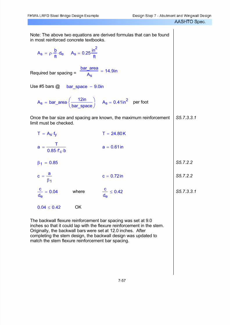
7/29/2019 LRFD steel design.pdf
http://slidepdf.com/reader/full/lrfd-steel-designpdf 400/646
The backwall flexure reinforcement bar spacing was set at 9.0
inches so that it could lap with the flexure reinforcement in the stem.Originally, the backwall bars were set at 12.0 inches. After completing the stem design, the backwall design was updated tomatch the stem flexure reinforcement bar spacing.
OK0.04 0.42≤
S5.7.3.3.1c
de0.42≤where
c
de0.04=
S5.7.2.2 c 0.72in=ca
β1
=
S5.7.2.2 β1 0.85=
a 0.61 in=aT
0.85 f'c⋅ b⋅=
T 24.80K=T As f y⋅=
S5.7.3.3.1Once the bar size and spacing are known, the maximum reinforcement
limit must be checked.
per foot As 0.41in2= As bar_area
12in
bar_space
⎛ ⎝
⎞ ⎠
⋅=
bar_space 9.0in=Use #5 bars @
Required bar spacing =bar_area
As14.9in=
As 0.25in
2
ft
= As ρb
ft
⋅ de⋅=
Note: The above two equations are derived formulas that can be foundin most reinforced concrete textbooks.
7-57
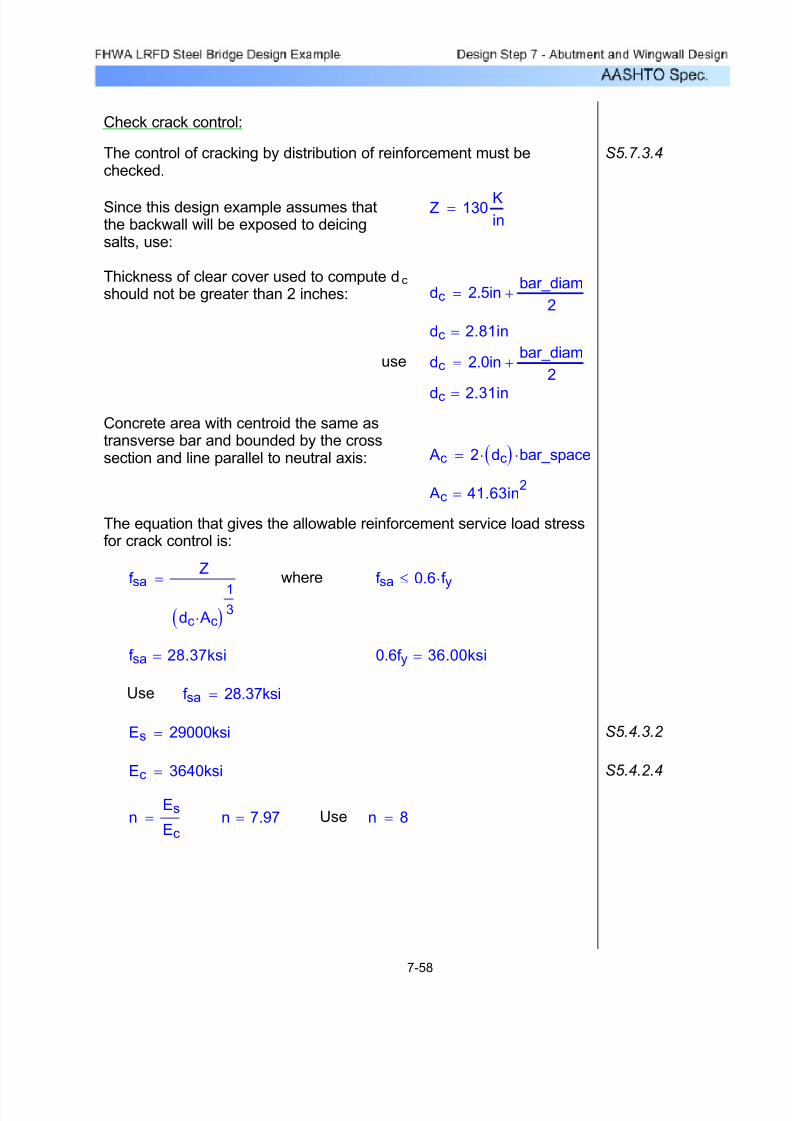
7/29/2019 LRFD steel design.pdf
http://slidepdf.com/reader/full/lrfd-steel-designpdf 401/646
n 8=Usen 7.97=nEs
Ec=
S5.4.2.4Ec 3640ksi=
S5.4.3.2 Es 29000ksi=
f sa 28.37ksi=Use
0.6f y 36.00ksi=f sa 28.37ksi=
f sa 0.6 f y⋅≤wheref saZ
dc Ac⋅( )13
=
The equation that gives the allowable reinforcement service load stressfor crack control is:
Ac 41.63in2=
Ac 2 dc( )⋅ bar_space⋅=
Concrete area with centroid the same astransverse bar and bounded by the crosssection and line parallel to neutral axis:
dc 2.31in=
dc 2.0inbar_diam
2+=use
dc 2.81in=
dc 2.5inbar_diam
2+=
Thickness of clear cover used to compute dc should not be greater than 2 inches:
Z 130 Kin
=Since this design example assumes thatthe backwall will be exposed to deicingsalts, use:
S5.7.3.4The control of cracking by distribution of reinforcement must bechecked.
Check crack control:
7-58

7/29/2019 LRFD steel design.pdf
http://slidepdf.com/reader/full/lrfd-steel-designpdf 402/646
Service backwall total load moment:
MubwservI 8.51K ft⋅ft
=
To solve for the actual stress in the reinforcement, the transformedmoment of inertia and the distance from the neutral axis to the centroidof the reinforcement must be computed:
de 17.19in= As 0.413in
2
ft= n 8=
ρ As
b
ftde⋅
= ρ 0.002=
k ρ n⋅( )2 2 ρ⋅ n⋅( )+ ρ n⋅−=
k 0.164=
k de⋅ 2.81in=
Neutral Axis
Front face of backwall at base
#5 bars
@ 9.0 inspacing
1 4
. 3 7 "
2 . 8
1 "
2 0
. 0 "
12.0"
2 . 8
1 "
Figure 7-12 Abutment Backwall Crack Control Check
7-59
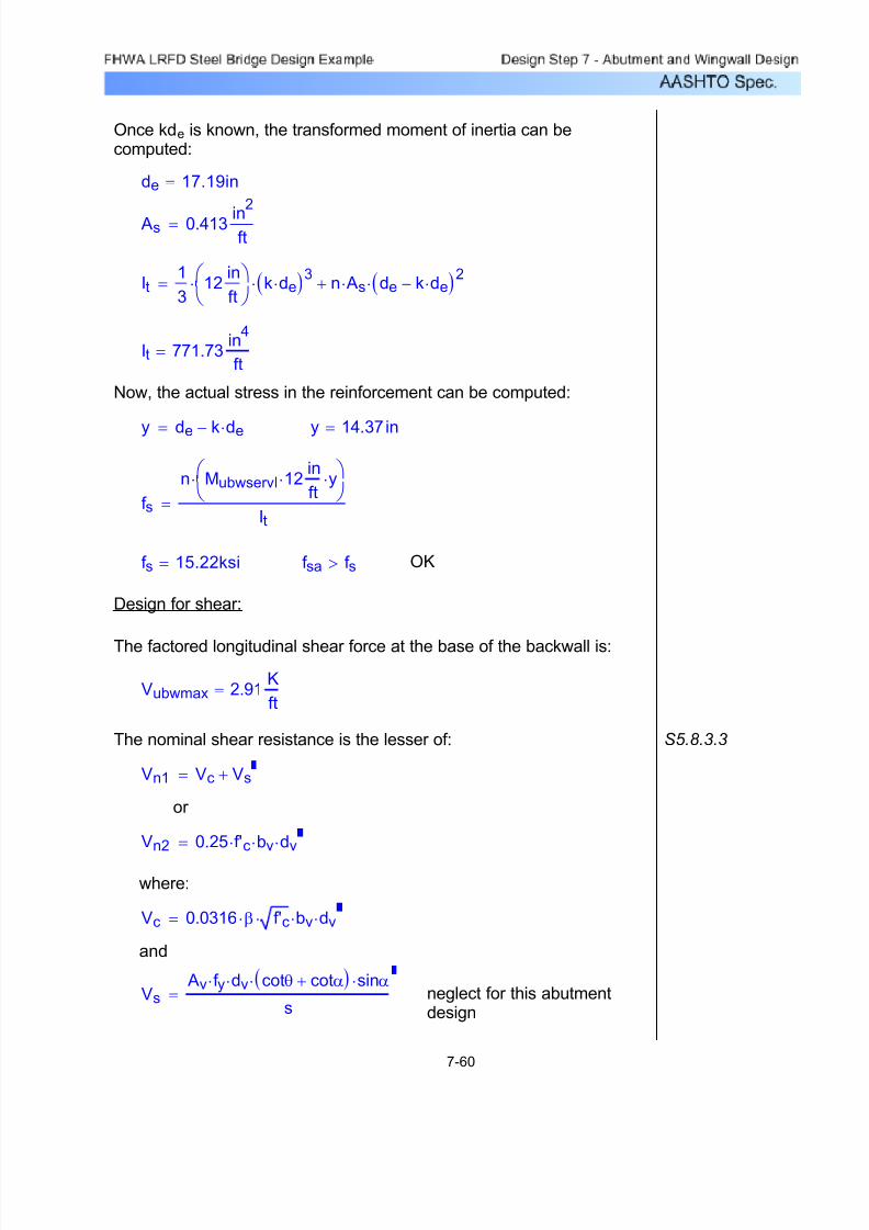
7/29/2019 LRFD steel design.pdf
http://slidepdf.com/reader/full/lrfd-steel-designpdf 403/646
neglect for this abutmentdesign
Vs Av f y⋅ dv⋅ cotθ cotα+( )⋅ sinα⋅
s=
and
Vc 0.0316 β⋅ f'c⋅ bv⋅ dv⋅=
where:
Vn2 0.25 f'c⋅ bv⋅ dv⋅=
or
Vn1 Vc Vs+=
S5.8.3.3The nominal shear resistance is the lesser of:
Vubwmax 2.91K
ft=
The factored longitudinal shear force at the base of the backwall is:
Design for shear:
OKf sa f s>f s 15.22ksi=
f s
n MubwservI 12⋅in
fty⋅⎛
⎝ ⎞ ⎠
⋅
It=
y 14.37 in=y de k de⋅−=
Now, the actual stress in the reinforcement can be computed:
It 771.73in
4
ft=
It1
312
in
ft
⎛ ⎝
⎞ ⎠
⋅ k de⋅( )3⋅ n As⋅ de k de⋅−( )2
⋅+=
As 0.413 in2
ft=
de 17.19in=
Once kde is known, the transformed moment of inertia can becomputed:
7-60

7/29/2019 LRFD steel design.pdf
http://slidepdf.com/reader/full/lrfd-steel-designpdf 404/646
OKVr Vubwmax>
Vr 22.93K
ft=
Vr φv Vn⋅=
S5.5.4.2.1φv 0.90=
The factored shear resistance is then:
Vn 25.48K
ft=Use:
K
ft
Vn2 201.60=
Vn2 0.25 f'c⋅ bv⋅ dv⋅=
K
ftVn1 25.48=
Vn1 0.0316 β⋅ f'c⋅ bv⋅ dv⋅=
ksif'c 4.0=For
Now, Vn1 and Vn2 can be calculated:
indv 16.80=
inh 20=
where:
S5.8.2.9dv max dea
2− 0.9 de⋅, 0.72 h⋅,⎛
⎝ ⎞ ⎠
=
inbv 12=
S5.8.3.4.1β 2.0=
Before the nominal shear resistance can be calculated, all thevariables used in the above equations need to be defined.
7-61

7/29/2019 LRFD steel design.pdf
http://slidepdf.com/reader/full/lrfd-steel-designpdf 405/646
Based on the backwall design, #5 bars at 9.0 inch spacing will beused for the back face flexure reinforcement. The same bar size andspacing will be used for the front face vertical reinforcement. Thehorizontal temperature and shrinkage reinforcement will consist of #4bars at 12.0 inch spacing for the front and back faces.
OK0.40in
2
ft0.36
in2
ft≥
As 0.40in
2
ft= As 2
bar_area
ft⋅=
bar_area 0.20in2=
bar_diam 0.500in=
Try 1 horizontal # 4 bar for each face of the backwall at 12.0 inchspacing:
The above steel must be distributed equally on both faces of the backwall.
As must be greater than or equal to 0.36in2/ft
in2
ft0.0015Ag 0.36=
or
in2
ft0.11
Ag
f y⋅ 0.44=
ksif y 60=
in2
ft Ag 240.0= Ag 20 in⋅( ) 12
in
ft⋅⎛
⎝ ⎞ ⎠
⋅=
Σ Ab 0.0015Ag=
or
As 0.11 Ag
fy≥
S5.10.8.2 For members less than 48.0 inches thick, the area of reinforcement ineach direction shall not be spaced greater than 12.0 inches and satisfythe lesser of:
S5.10.8 Shrinkage and temperature reinforcement:
7-62
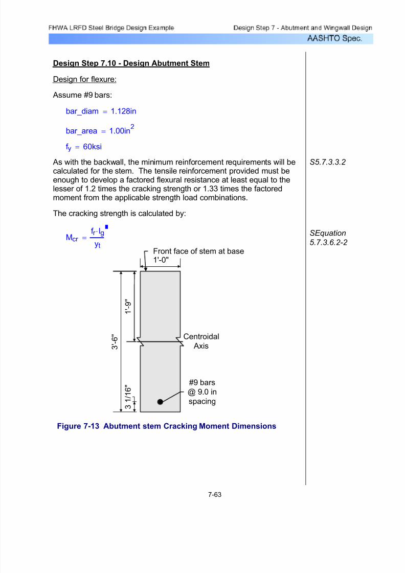
7/29/2019 LRFD steel design.pdf
http://slidepdf.com/reader/full/lrfd-steel-designpdf 406/646
Design Step 7.10 - Design Abutment Stem
Design for flexure:
Assume #9 bars:
bar_diam 1.128in=
bar_area 1.00in2
=
f y 60ksi=
As with the backwall, the minimum reinforcement requirements will becalculated for the stem. The tensile reinforcement provided must beenough to develop a factored flexural resistance at least equal to thelesser of 1.2 times the cracking strength or 1.33 times the factored
moment from the applicable strength load combinations.
S5.7.3.3.2
The cracking strength is calculated by:
SEquation
5.7.3.6.2-2 Mcr
f r Ig⋅
yt=
Centroidal
Axis
Front face of stem at base
#9 bars
@ 9.0 in
spacing
3 ' - 6 "
1 ' - 9 "
3 1
/ 1 6 "
1'-0"
Figure 7-13 Abutment stem Cracking Moment Dimensions
7-63
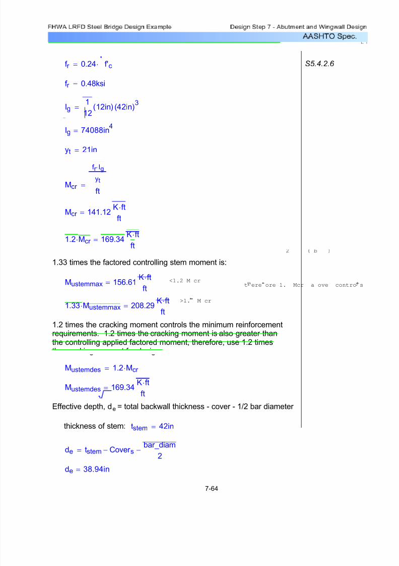
7/29/2019 LRFD steel design.pdf
http://slidepdf.com/reader/full/lrfd-steel-designpdf 407/646
de 38.94in=
de tstem Cover s−bar_diam
2−=
tstem 42in=thickness of stem:
Effective depth, de = total backwall thickness - cover - 1/2 bar diameter
Mustemdes 169.34K ft⋅
ft
=
Mustemdes 1.2 Mcr ⋅=
1.2 times the cracking moment controls the minimum reinforcementrequirements. 1.2 times the cracking moment is also greater thanthe controlling applied factored moment, therefore, use 1.2 timesthe cracking moment for design.
1.33 Mustemmax⋅ 208.29K ft⋅ft
=
Mustemmax 156.61K ft⋅ft
=
1.33 times the factored controlling stem moment is:
1.2 Mcr ⋅ 169.34K ft⋅ft
=
Mcr 141.12K ft⋅ft
=
Mcr
f r Ig⋅
yt
ft=
yt 21in=
Ig 74088in4
=
Ig1
1212in( ) 42in( )
3=
f r 0.48ksi=
S5.4.2.6 f r 0.24 f'c⋅=
7-64
<1.2 M cr
>1. M cr
t ere ore 1. Mcr a ove contro s
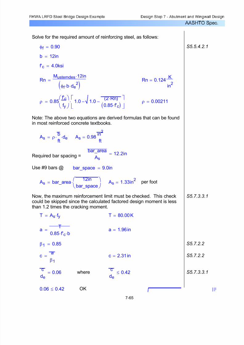
7/29/2019 LRFD steel design.pdf
http://slidepdf.com/reader/full/lrfd-steel-designpdf 408/646
per foot
Now, the maximum reinforcement limit must be checked. This checkcould be skipped since the calculated factored design moment is lessthan 1.2 times the cracking moment.
S5.7.3.3.1
T As f y⋅= T 80.00K=
aT
0.85 f'c⋅ b⋅= a 1.96 in=
β1 0.85= S5.7.2.2
ca
β1
= c 2.31in= S5.7.2.2
c
de0.06= where
c
de0.42≤ S5.7.3.3.1
0.06 0.42≤ OK
Solve for the required amount of reinforcing steel, as follows:
φf 0.90= S5.5.4.2.1
b 12in=
f'c 4.0ksi=
RnMustemdes 12⋅ in
φf b⋅ de2⋅( )
= Rn 0.124K
in2
=
ρ 0.85f'c
f y
⎛
⎝
⎞
⎠1.0 1.0
2 Rn⋅( )
0.85 f'c⋅( )−−
⎡
⎣
⎤
⎦⋅= ρ 0.00211=
Note: The above two equations are derived formulas that can be foundin most reinforced concrete textbooks.
As ρb
ft⋅ de⋅= As 0.98
in2
ft=
bar_area
As12.2in=Required bar spacing =
Use #9 bars @ bar_space 9.0in=
As bar_area 12inbar_space⎛ ⎝ ⎞ ⎠⋅= As 1.33in2=
7-65

7/29/2019 LRFD steel design.pdf
http://slidepdf.com/reader/full/lrfd-steel-designpdf 409/646
n 8=Usen 7.97=nEs
Ec=
S5.4.2.4Ec 3640ksi=
S5.4.3.2 Es 29000ksi=
f sa 26.48ksi=Use
0.6f y 36.00ksi=f sa 26.48ksi=
f sa 0.6 f y⋅≤wheref sa Z
dc Ac⋅( )
1
3
=
The equation that gives the allowable reinforcement service load stressfor crack control is:
Ac 46.15in2=
Ac 2 dc( )⋅ bar_space⋅=
Concrete area with centroid the same astransverse bar and bounded by the crosssection and line parallel to neutral axis:
dc 2.56in=
dc 2.0inbar_diam
2+=use
dc 3.06in=
dc 2.5inbar_diam
2+=
Thickness of clear cover used to compute dc should not be greater than 2 inches:
Z 130K
in=Since this design example assumes that the
abutment stem will be exposed to deicingsalts, use:
S5.7.3.4The control of cracking by distribution of reinforcement must bechecked.
Check crack control:
7-66

7/29/2019 LRFD steel design.pdf
http://slidepdf.com/reader/full/lrfd-steel-designpdf 410/646
Stem factored service moment:
MustemservI 105.82K ft⋅ft
=
To solve for the actual stress in the reinforcement, the transformedmoment of inertia and the distance from the neutral axis to the centroidof the reinforcement must be computed:
de 38.94in= As 1.33in
2
ft= n 8=
ρ As
b
ftde⋅
= ρ 0.00285=
k ρ n⋅( )22 ρ⋅ n⋅( )+ ρ n⋅−=
k 0.192=
k de⋅ 7.47in=
Neutral
Axis
Front face of stem at base
#9 bars
@ 9.0 in
spacing
7 . 4 7 "
3 1
. 4 7 "
4 2
. 0 0 "
12"
3 . 0
6 "
Figure 7-14 Abutment Stem Crack Control Check
7-67

7/29/2019 LRFD steel design.pdf
http://slidepdf.com/reader/full/lrfd-steel-designpdf 411/646
neglect for this abutmentdesign
Vs Av f y⋅ dv⋅ cotθ cotα+( )⋅ sinα⋅
s=
and
Vc 0.0316 β⋅ f'c⋅ bv⋅ dv⋅=
where:
Vn2 0.25 f'c⋅ bv⋅ dv⋅=
or
Vn1 Vc Vs+=
S5.8.3.3The nominal shear resistance is the lesser of:
Vustemmax 16.03K
ft=
The factored longitudinal shear force at the base of the stem is:
Design for shear:
OKf sa f s>f s 26.20ksi=
f s
n MustemservI 12⋅in
fty⋅⎛
⎝ ⎞ ⎠
⋅
It=
y 31.47 in=y de k de⋅−=
Now, the actual stress in the reinforcement can be computed:
It 12202.09in
4
ft=
It1
312
in
ft
⎛ ⎝
⎞ ⎠
⋅ k de⋅( )3⋅ n As⋅ de k de⋅−( )2
⋅+=
As 1.330in2
ft=
de 38.94in=
Once kde is known, the transformed moment of inertia can becomputed:
7-68

7/29/2019 LRFD steel design.pdf
http://slidepdf.com/reader/full/lrfd-steel-designpdf 412/646
OKVr Vustemmax>
Vr 52.15K
ft=
Vr φv Vn⋅=
S5.5.4.2.1φv 0.90=
The factored shear resistance is then:
Vn 57.94K
ft=use
K
ftVn2 458.40=
Vn2 0.25 f'c⋅ bv⋅ dv⋅=
K
ftVn1 57.94=
Vn1 0.0316 β⋅ f'c⋅ bv⋅ dv⋅=
ksif'c 4.0=For
Now, Vn1 and Vn2 can be calculated:
indv 38.2=
inh 42=
where:
S5.8.2.9dv max dea
2− 0.9 de⋅, 0.72 h⋅,⎛
⎝ ⎞ ⎠
=
inbv 12=
S5.8.3.4.1β 2.0=
Before the nominal shear resistance can be calculated, all thevariables used in the above equations need to be defined.
7-69

7/29/2019 LRFD steel design.pdf
http://slidepdf.com/reader/full/lrfd-steel-designpdf 413/646
Based on the abutment stem design, #9 bars at 9.0 inch spacing willbe used for the back face flexure reinforcement. The same bar sizeand spacing will be used for the front face vertical reinforcement toreduce design steps. The horizontal temperature and shrinkagereinforcement will consist of #5 bars at 9.0 inch spacing for the frontand back faces.
OK0.83in
2
ft0.76
in2
ft≥
As 0.83in
2
ft= As 2
bar_area12in
9in
⎛ ⎝
⎞ ⎠
⋅
ft⋅=
bar_area 0.31in2
=
bar_diam 0.625in=
Try 1 horizontal # 5 bar for each face of the stem at 9.0 inch spacing:
The above steel must be distributed equally on both faces of the stem.
As must be greater than or equal to 0.76in2/ft
in2
ft0.0015Ag 0.76=
or
in2
ft0.11
Ag
f y⋅ 0.92=
ksif y 60=
in2
ft Ag 504.0= Ag 42 in⋅( ) 12
in
ft⋅⎛
⎝ ⎞ ⎠
⋅=
Σ Ab 0.0015Ag=
or
As 0.11 Ag
fy≥
S5.10.8.2 For members less than 48.0 inches thick, the area of reinforcement ineach direction shall not be spaced greater than 12.0 inches and satisfythe lesser of:
S5.10.8 Shrinkage and temperature reinforcement:
7-70

7/29/2019 LRFD steel design.pdf
http://slidepdf.com/reader/full/lrfd-steel-designpdf 414/646
Design Step 7.11 - Design Abutment Footing
The abutment footing is designed for flexure in the heel and toe,one-way and two-way shear action, and the control of cracking by the
distribution of reinforcement. For footings supported by pilefoundations, the footing and pile foundation designs areinterdependent and should be designed concurrently to be moreefficient. Refer to Design Step P for the pile foundation design.
S5.13.3
S5.7.3.4
The following figures show the assumed footing dimensions and pilelocations within the footing.
7-71

7/29/2019 LRFD steel design.pdf
http://slidepdf.com/reader/full/lrfd-steel-designpdf 415/646
4 6 ' - 1 0 1 / 2 "
1'-3" 1'-3"
5'-1 1/2"
2 3 ' - 5 1 / 4 "
5'-9"
L abutment
stem
C
7'-9"
7 ' - 4 "
7 ' - 4 "
Abutment
footing toe
7 1/2"
L footing and
pile group
(longitudinal
axis)
C
L footing and pile
group (transverse
axis)
C
10'-3"
HP12x53
(Typ.) Gr.
50 steel
1 ' - 5 1 / 4 "
7 ' - 4 "
7 ' - 4 "
7 ' - 4 "
7 ' - 4 "
1 ' - 5 1 / 4 "
Abutment
footing heel
Legend:
Battered Pile
Vertical Pile
1 2
3
5
7
9
11 12
8
6
4
10
13 14
Figure 7-15 Abutment Footing and Pile Foundation Plan View
7-72

7/29/2019 LRFD steel design.pdf
http://slidepdf.com/reader/full/lrfd-steel-designpdf 416/646
10'-3"
3'-6"
2 ' - 6 "2'-9"4'-0"
1'-3" 1
3
1'-3" 1 ' - 0 "
Heel
Toe
Abutment
stem
Figure 7-16 Abutment Footing and Pile Foundation Elevation View
Design for flexure:
The flexure reinforcement must be designed at two critical sections for abutment footings. The two sections include the back and front face of the stem. The moments at the abutment faces are calculated from thepile reactions.
S5.13.3.4
7-73
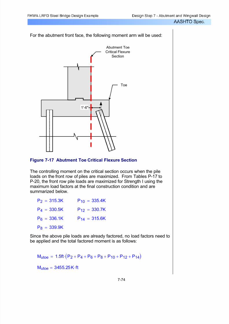
7/29/2019 LRFD steel design.pdf
http://slidepdf.com/reader/full/lrfd-steel-designpdf 417/646
For the abutment front face, the following moment arm will be used:
1'-6"
Toe
Abutment Toe
Critical Flexure
Section
Figure 7-17 Abutment Toe Critical Flexure Section
The controlling moment on the critical section occurs when the pileloads on the front row of piles are maximized. From Tables P-17 toP-20, the front row pile loads are maximized for Strength I using themaximum load factors at the final construction condition and aresummarized below.
P2 315.3K= P10 335.4K=
P4 330.5K= P12 330.7K=
P6 336.1K= P14 315.6K=
P8 339.9K=Since the above pile loads are already factored, no load factors need tobe applied and the total factored moment is as follows:
Mutoe 1.5ft P2 P4+ P6+ P8+ P10+ P12+ P14+( )⋅=
Mutoe 3455.25K ft⋅=
7-74
7/29/2019 LRFD steel design.pdf
http://slidepdf.com/reader/full/lrfd-steel-designpdf 418/646
The moment on a per foot basis is then:
MutoeftMutoe
Labut=
Mutoeft 73.71Kft
ft⋅=
Once the maximum moment at the critical section is known, the sameprocedure that was used for the backwall and stem to calculate theflexure reinforcement must be followed. The footing toe flexurereinforcement is located longitudinally in the bottom of the footingsince the bottom of footing is in tension at the critical toe section.These bars will extend from the back of the heel to the front of the toetaking into account the clear cover:
Assume #8 bars:
bar_diam 1.000in=
bar_area 0.79in2=
f y 60ksi=
The footing toe critical section minimum tensile reinforcementrequirements will be calculated. The tensile reinforcement providedmust be enough to develop a factored flexural resistance at leastequal to the lesser of 1.2 times the cracking strength or 1.33 times thefactored moment from the applicable strength load combinations.
S5.7.3.3.2
The cracking strength is calculated by:
SEquation
5.7.3.6.2-2 Mcr
f r Ig⋅
yt=
7-75
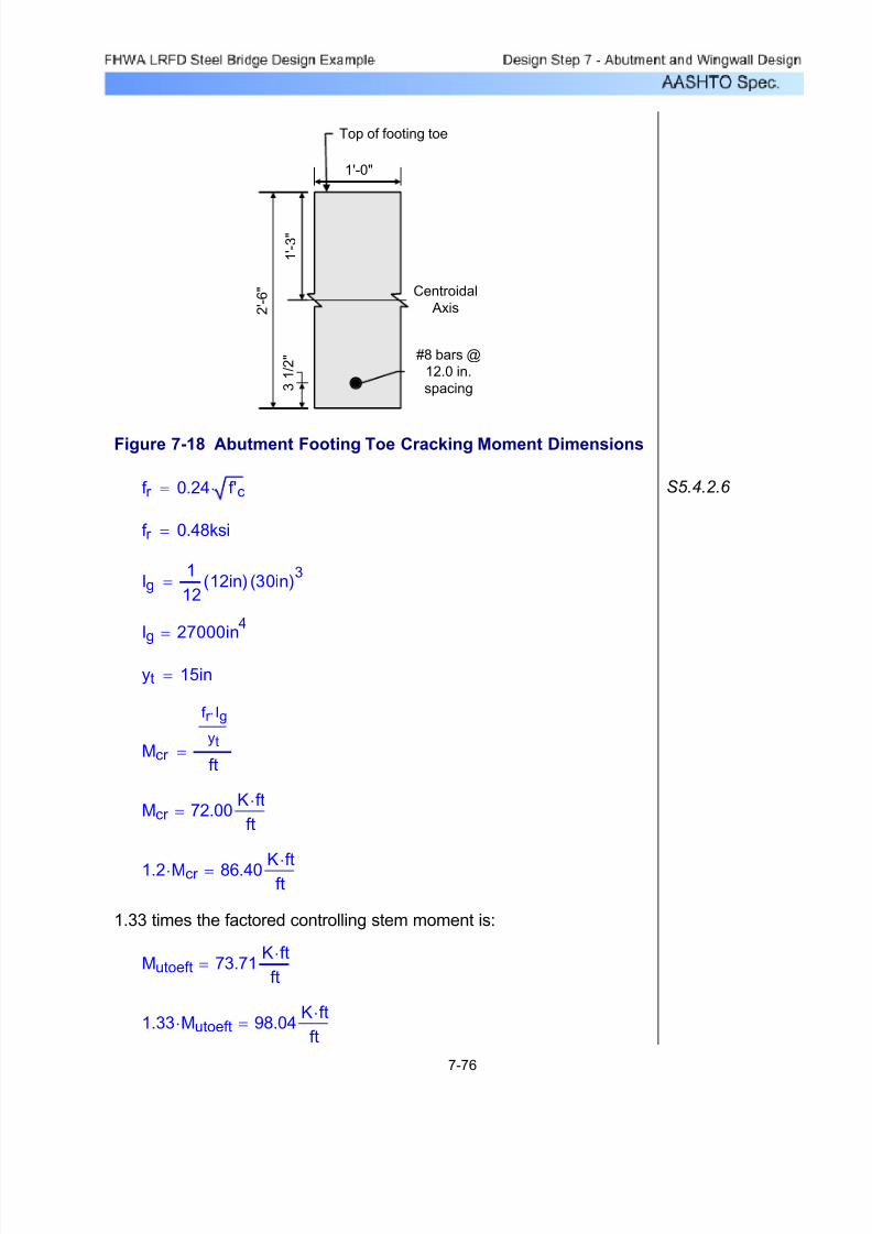
7/29/2019 LRFD steel design.pdf
http://slidepdf.com/reader/full/lrfd-steel-designpdf 419/646
Centroidal
Axis
Top of footing toe
#8 bars @
12.0 in.
spacing
2 ' - 6 "
1 ' - 3 "
3 1 / 2 "
1'-0"
Figure 7-18 Abutment Footing Toe Cracking Moment Dimensions
f r 0.24 f'c⋅= S5.4.2.6
f r 0.48ksi=
Ig1
1212in( ) 30in( )
3=
Ig 27000in4
=
yt 15in=
Mcr
f r Ig⋅
yt
ft=
Mcr 72.00K ft⋅ft
=
1.2 Mcr ⋅ 86.40 K ft⋅ft
=
1.33 times the factored controlling stem moment is:
Mutoeft 73.71K ft⋅ft
=
1.33 Mutoeft⋅ 98.04K ft⋅ft
=
7-76

7/29/2019 LRFD steel design.pdf
http://slidepdf.com/reader/full/lrfd-steel-designpdf 420/646
Required bar spacing =bar_area
As12.8in=
As 0.74in
2
ft= As ρ
b
ft⋅ de⋅=
Note: The above two equations are derived formulas that can be foundin most reinforced concrete textbooks.
ρ 0.00233=
ρ 0.85f'c
f y
⎛
⎝
⎞
⎠1.0 1.0
2 Rn⋅( )
0.85 f'c⋅( )−−
⎡⎣
⎤⎦
⋅=
Rn 0.137K
in2
=RnMufttoedes 12⋅ in
φf b⋅ de2
⋅( )=
f'c 4.0ksi=
b 12in=
S5.5.4.2.1φf 0.90=
Solve for the required amount of reinforcing steel, as follows:
de 26.50in=
de tftg Cover fb−bar_diam
2−=
Cover fb 3.00in=
tftg 30in=thickness of footing:
Effective depth, de = total footing thickness - cover - 1/2 bar diameter
Mufttoedes 86.40K ft⋅ft
=
Mufttoedes 1.2 Mcr ⋅=
1.2 times the cracking moment controls the minimum reinforcementrequirements. 1.2 times the cracking moment is also greater thanthe factored footing toe moment. Therefore, use 1.2 times thecracking moment to design the toe flexure reinforcement.
7-77

7/29/2019 LRFD steel design.pdf
http://slidepdf.com/reader/full/lrfd-steel-designpdf 421/646
c
de0.42≤ S5.7.3.3.1
0.05 0.42≤ OK
Check crack control:
The control of cracking by distribution of reinforcement must bechecked for the abutment toe. S5.7.3.4
Since the footing is buried, moderateexposure will be assumed, use:
Z 170K
in=
Thickness of clear cover used to compute dc should not be greater than 2 inches: dc 3.0in
bar_diam
2+=
dc 3.50in=
use dc 2.0in bar_diam2
+=
dc 2.50in=
Concrete area with centroid the same astransverse bar and bounded by the crosssection and line parallel to neutral axis: Ac 2 dc( )⋅ bar_space⋅=
Ac 60.00in2=
Use #8 bars @ bar_space 12.0in=
As bar_area12in
bar_space
⎛ ⎝
⎞ ⎠
⋅= As 0.79in2= per foot
Once the bar size and spacing are known, the maximum reinforcementlimit must be checked.
S5.7.3.3.1
T As f y⋅= T 47.40K=
aT
0.85 f'c⋅ b⋅= a 1.16in=
β1 0.85= S5.7.2.2
c aβ1
= c 1.37 in= S5.7.2.2
c
de0.05= where
7-78
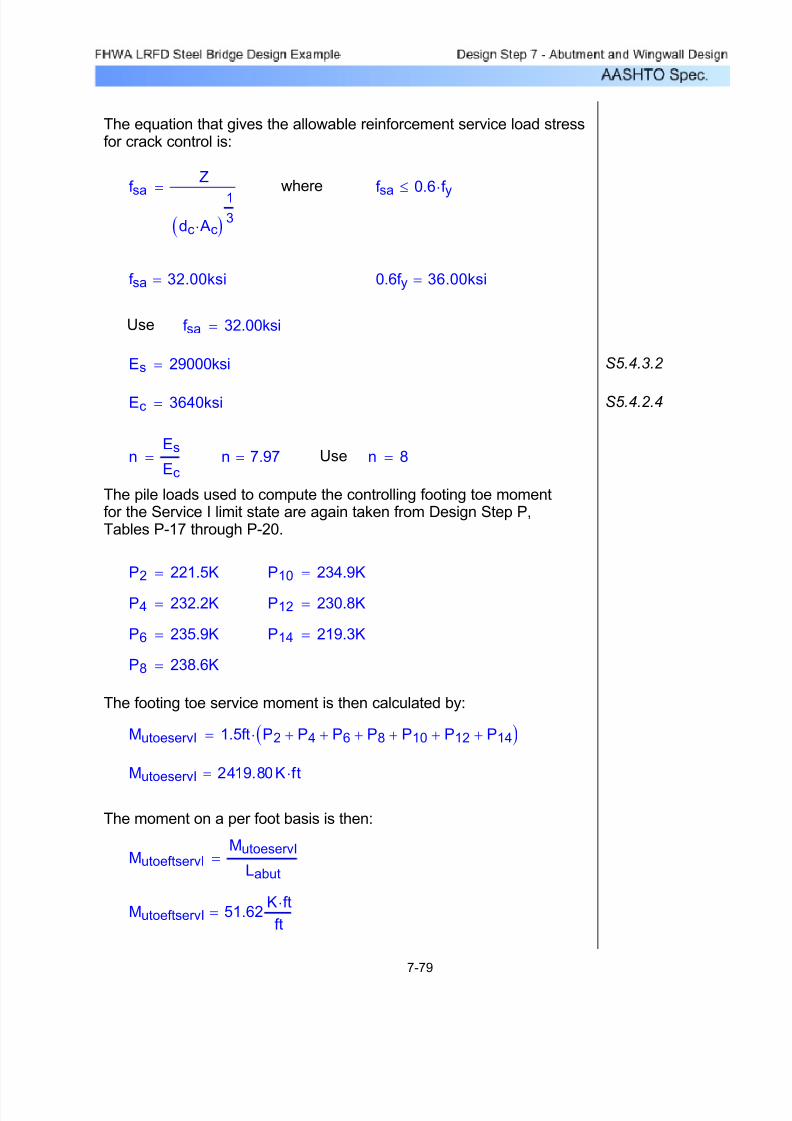
7/29/2019 LRFD steel design.pdf
http://slidepdf.com/reader/full/lrfd-steel-designpdf 422/646
MutoeftservI 51.62K ft⋅ft
=
MutoeftservIMutoeservI
Labut=
The moment on a per foot basis is then:
MutoeservI 2419.80K ft⋅=
MutoeservI 1.5ft P2 P4+ P6+ P8+ P10+ P12+ P14+( )⋅=
The footing toe service moment is then calculated by:
P8 238.6K=
P14 219.3K=P6 235.9K=
P12 230.8K=P4 232.2K=
P10 234.9K=P2 221.5K=
The pile loads used to compute the controlling footing toe momentfor the Service I limit state are again taken from Design Step P,Tables P-17 through P-20.
n 8=Usen 7.97=nEs
Ec=
S5.4.2.4Ec 3640ksi=
S5.4.3.2 Es 29000ksi=
f sa 32.00ksi=Use
0.6f y 36.00ksi=f sa 32.00ksi=
f sa
0.6 f y
⋅≤wheref sa
Z
dc Ac⋅( )1
3
=
The equation that gives the allowable reinforcement service load stressfor crack control is:
7-79

7/29/2019 LRFD steel design.pdf
http://slidepdf.com/reader/full/lrfd-steel-designpdf 423/646
To solve for the actual stress in the reinforcement, the transformedmoment of inertia and the distance from the neutral axis to the centroidof the reinforcement must be computed:
de 26.50in= As .79 in2
ft= n 8=
ρ As
b
ftde⋅
= ρ 0.00248=
k ρ n⋅( )22 ρ⋅ n⋅( )+ ρ n⋅−=
k 0.180=
k de⋅ 4.78in=
3 0 . 0 0 "
Neutral
Axis
Top of footing toe
#8 bars @
12.0 in
spacing
4 . 7
8 "
2 1
. 7 2
"
12"
3 . 5
0 "
Figure 7-19 Abutment Footing Toe Crack Control Check
7-80

7/29/2019 LRFD steel design.pdf
http://slidepdf.com/reader/full/lrfd-steel-designpdf 424/646
Once kde is known, the transformed moment of inertia can becomputed:
de 26.50in=
As 0.790in2
ft=
It1
312
in
ft
⎛ ⎝
⎞ ⎠
⋅ k de⋅( )3⋅ n As⋅ de k de⋅−( )2
⋅+=
It 3418.37in
4
ft=
Now, the actual stress in the reinforcement can be computed:
y de k de⋅−= y 21.72 in=
f s
n MutoeftservI 12⋅in
fty⋅⎛
⎝ ⎞ ⎠
⋅
It=
f s 31.48ksi= f sa f s> OK
7-81

7/29/2019 LRFD steel design.pdf
http://slidepdf.com/reader/full/lrfd-steel-designpdf 425/646
For the abutment back face flexure design, the following moment armwill be used:
10'-3"
2 ' - 6 "2'-9"4'-0"
1'-3" 1
3
2'-9" 1 ' - 0 "
Heel
Toe
Abutment Heel
Critical Flexure
Section
Figure 7-20 Abutment Heel Critical Flexure Section
The controlling moment on the critical section occurs when the pileloads on the back row of piles are minimized. From Tables P-17 toP-20, the back row pile loads are minimized for Strength I using theminimum load factors at the final construction condition and aresummarized below. Piles in tension are shown as having negative pileloads.
P1 15.3− K= P9 14.5− K=
P3 14.8− K= P11 14.8− K=
P5 14.5− K= P13 15.3− K=
P7 14.4− K=
Since the above pile loads are already factored, no load factors need tobe applied and the total factored moment is as follows:
Muheel 2.75ft P1 P3+ P5+ P7+ P9+ P11+ P13+( )⋅=
Muheel 284.90− K ft⋅=
7-82

7/29/2019 LRFD steel design.pdf
http://slidepdf.com/reader/full/lrfd-steel-designpdf 426/646
The moment on a per foot basis is then:
MuheelftMuheel
Labut=
Muheelft 6.08− Kft
ft⋅=
Once the moment at the critical section is known, the same procedurethat was used for the toe must be followed. The flexure reinforcementfor the footing heel is placed longitudinally along the top of the footingsince the top of the footing heel is in tension at the critical heel section.The bars will extend from the back of the heel to the front of the toetaking into account the concrete cover.
Assume #5 bars:
bar_diam 0.625in=
bar_area 0.31in2
=
f y 60ksi=
The footing heel critical section minimum tensile reinforcementrequirements will be calculated. The tensile reinforcement providedmust be enough to develop a factored flexural resistance at leastequal to the lesser of 1.2 times the cracking strength or 1.33 times thefactored moment from the applicable strength load combinations.
S5.7.3.3.2
The cracking strength is calculated by:
SEquation
5.7.3.6.2-2 Mcr f r Ig⋅
yt=
7-83

7/29/2019 LRFD steel design.pdf
http://slidepdf.com/reader/full/lrfd-steel-designpdf 427/646
Centroidal
Axis
Top of footing heel
#5 bars @
12.0 in
spacing
2 ' - 6 "
1 ' - 3 "
2 5 / 1 6 "
1'-0"
Figure 7-21 Abutment Footing Heel Cracking Moment Dimensions
f r 0.24 f'c⋅= S5.4.2.6
f r 0.48ksi=
Ig1
1212in( ) 30in( )
3=
Ig 27000in4=
yt 15in=
Mcr
f r − Ig⋅
yt
ft=
Mcr 72.00−K ft⋅ft
=
1.2 Mcr ⋅ 86.40−K ft⋅ft
=
1.33 times the factored controlling heel moment is:
1.33 Muheelft⋅ 8.08−K ft⋅ft
=
7-84
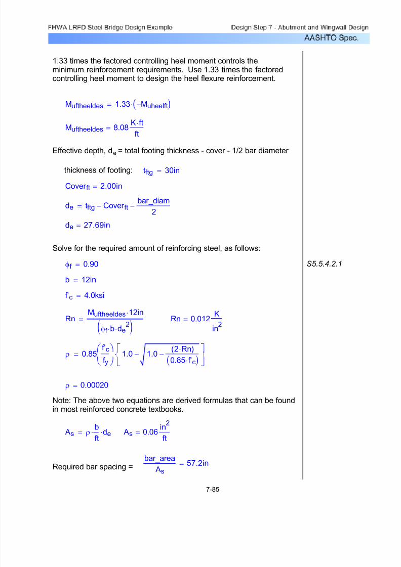
7/29/2019 LRFD steel design.pdf
http://slidepdf.com/reader/full/lrfd-steel-designpdf 428/646
Required bar spacing =bar_area
As57.2in=
As 0.06in
2
ft= As ρ
b
ft⋅ de⋅=
Note: The above two equations are derived formulas that can be foundin most reinforced concrete textbooks.
ρ 0.00020=
ρ 0.85f'c
f y
⎛
⎝
⎞
⎠1.0 1.0
2 Rn⋅( )
0.85 f'c⋅( )−−
⎡⎣
⎤⎦
⋅=
Rn 0.012K
in2
=RnMuftheeldes 12⋅ in
φf b⋅ de2
⋅( )=
f'c 4.0ksi=
b 12in=
S5.5.4.2.1φf 0.90=
Solve for the required amount of reinforcing steel, as follows:
de 27.69in=
de tftg Cover ft− bar_diam
2−=
Cover ft 2.00in=
tftg 30in=thickness of footing:
Effective depth, de = total footing thickness - cover - 1/2 bar diameter
Muftheeldes 8.08K ft⋅ft
=
Muftheeldes 1.33 Muheelft−( )⋅=
1.33 times the factored controlling heel moment controls theminimum reinforcement requirements. Use 1.33 times the factoredcontrolling heel moment to design the heel flexure reinforcement.
7-85

7/29/2019 LRFD steel design.pdf
http://slidepdf.com/reader/full/lrfd-steel-designpdf 429/646
Preliminary Design
A quick way to come up with a design section that willprobably work for all design checks is to just check thecrack control requirements for LRFD. It has been thedesigner's experience that in many footing designs,the crack control requirements control the footingdesign. The above is true for LRFD because LFDallows a certain percentage of overstress for the
service cases due to the low probability that the loadscombined for each service case will actually occur simultaneously.
The crack control check for the footing heel critical section will not becarried out. The calculations are similar to that of the abutment
backwall, stem, and footing toe.
OK0.05 0.42≤
S5.7.3.3.1c
de0.42≤where
c
de0.02=
S5.7.2.2 c 0.54 in=c aβ1
=
S5.7.2.2 β1 0.85=
a 0.46in=aT
0.85 f'c⋅ b⋅=
T 18.60K=T As f y⋅=
S5.7.3.3.1Once the bar size and spacing are known, the maximum reinforcementlimit must be checked.
per foot As 0.31in2= As bar_area
12in
bar_space
⎛ ⎝
⎞ ⎠
⋅=
bar_space 12.0in=Use #5 bars @
7-86
7/29/2019 LRFD steel design.pdf
http://slidepdf.com/reader/full/lrfd-steel-designpdf 430/646
OK0.31in
2
ft0.27
in2
ft≥
As 0.31 in2
ft= As
bar_area12in
12in
⎛
⎝
⎞
⎠⋅
ft=
bar_area 0.31in2=
bar_diam 0.625in=
Try 1 # 5 bar at 12.0 inch spacing for one face:
Astop 0.27in
2
ft= Astop
0.54 in2
ft
2=
For one face only:
The total combined amount of reinforcing steel on the top and
bottom transverse faces must be greater than or equal to 0.54 in2/ft.
in2
ft0.0015Ag 0.54=
or
in2
ft0.11
Ag
f y⋅ 0.66=
ksif y 60=
in2
ft Ag 360.00= Ag 30 in⋅( ) 12
in
ft⋅⎛
⎝ ⎞ ⎠
⋅=
Σ Ab 0.0015Ag=or As 0.11 Ag
fy≥
S5.10.8.2 For members less than 48.0 inches thick, the area of reinforcement ineach direction shall not be spaced greater than 12.0 inches and satisfythe lesser of:
S5.10.8 Shrinkage and temperature reinforcement:
7-87

7/29/2019 LRFD steel design.pdf
http://slidepdf.com/reader/full/lrfd-steel-designpdf 431/646
indv 25.92=use
indv 25.92=or in0.5 dv⋅ cot θ( )⋅ 12.96=
Now the critical section can be calculated:
dv 25.92=
inh 30=
taken from footing toe strength flexure designina 1.16=
taken from footing toe strength flexure design
Based on the abutment footing flexure design, #8 bars at 12.0 inchspacing are required for the bottom longitudinal flexure reinforcement.#5 bars at 12.0 inch spacing are required for the top longitudinalflexure reinforcement. In the footing transverse direction, the shrinkageand temperature reinforcement calculations require #5 bars at 12.0inch spacing for the top and bottom mats.
Design for shear: S5.13.3.6
Shear design in abutment footings consists of having adequateresistance against one-way action and two-way action. For bothone-way and two-way actions, the design shear is taken at a criticalsection. For abutments, one-way action is checked in the toe and heel.The factored shear force at the critical section is computed by cutting
the footing at the critical section and summing the pile loads or portionsof pile loads that are outside the critical section. Two-way action inabutment footings supported by piles is generally checked taking a
critical perimeter around individual piles or around a group of pileswhen the critical perimeter of individual piles overlap.
For one way action in the abutment footing toe, the critical section istaken as the larger of:
S5.13.3.6.1 &
S5.8.3.2
0.5 dv⋅ cotθ⋅ or dv
θ 45deg=
The term dv is calculated the same as it is for the backwall and stem:
dv max dea
2− 0.9 de⋅, 0.72 h⋅,⎛
⎝ ⎞ ⎠
= S5.8.2.9
where:
de 26.50= in
7-88
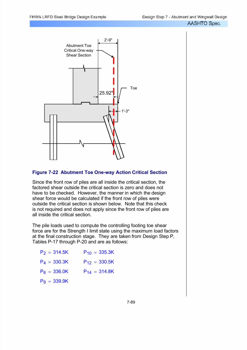
7/29/2019 LRFD steel design.pdf
http://slidepdf.com/reader/full/lrfd-steel-designpdf 432/646
1'-3"
Toe
Abutment Toe
Critical One-way
Shear Section
2'-9"
25.92"
Figure 7-22 Abutment Toe One-way Action Critical Section
Since the front row of piles are all inside the critical section, thefactored shear outside the critical section is zero and does nothave to be checked. However, the manner in which the designshear force would be calculated if the front row of piles wereoutside the critical section is shown below. Note that this checkis not required and does not apply since the front row of piles areall inside the critical section.
The pile loads used to compute the controlling footing toe shear force are for the Strength I limit state using the maximum load factorsat the final construction stage. They are taken from Design Step P,Tables P-17 through P-20 and are as follows:
P2 314.5K= P10 335.3K=
P4 330.3K= P12 330.5K=
P6 336.0K= P14 314.8K=
P8 339.9K=
7-89

7/29/2019 LRFD steel design.pdf
http://slidepdf.com/reader/full/lrfd-steel-designpdf 433/646
bv 12= in
dv 25.92= in S5.8.2.9
Now, Vn1 and Vn2 can be calculated:
For f'c 4.0= ksi
Vn1 0.0316 β⋅ f'c⋅ bv⋅ dv⋅=
Vn1 39.32= Kft
Vn2 0.25 f'c⋅ bv⋅ dv⋅=
Vn2 311.04=K
ft
Use: Vn 39.32K
ft=
The factored one-way shear force at the abutment footing toe criticalsection on a per foot basis is then:
VuftgtoeP2 P4+ P6+ P8+ P10+ P12+ P14+( )
Labut
=
Vuftgtoe 49.09K
ft=
The nominal shear resistance is the lesser of: S5.8.3.3
Vn1 Vc Vs+=
or
Vn2 0.25 f'c⋅ bv⋅ dv⋅=
where:
Vc 0.0316 β⋅ f'c⋅ bv⋅ dv⋅=
and
Vs Av f y⋅ dv⋅ cotθ cotα+( )⋅ sinα⋅
s= neglect for this abutment
design
Before the nominal shear resistance can be calculated, all thevariables used in the above equations need to be defined.
β 2.0= S5.8.3.4.1
7-90

7/29/2019 LRFD steel design.pdf
http://slidepdf.com/reader/full/lrfd-steel-designpdf 434/646
indv 25.92=
inh 30=
use the same stress block depth as thetoe - conservative
ina 1.16=
use the same effective depth as thetoe - conservative
inde 26.50=
where:
S5.8.2.9dv max dea
2− 0.9 de⋅, 0.72 h⋅,⎛
⎝ ⎞ ⎠
=
The term dv is calculated the same as it is for the abutment toe:
S5.13.3.6.1 &
C5.13.3.6.1
For one way action in the abutment footing heel, the critical section istaken at the abutment face for heels that are in tension on the topface of the heel. For heels that are in compression on the top face,
the critical section is calculated according to S5.8.2.9. Themaximum factored abutment footing heel shear occurs when the heelis in tension on the top face. Therefore, the critical section is takenat the stem back face.
If the front row of piles were outside the critical section, the one-wayshear for the abutment footing toe would fail. The footing depth wouldhave to be increased or the piles would have to be redesigned toreduce the shear force outside the critical section. Again, the above
design shear force and resistance are just shown to illustrate the toeone-way shear check if the pile loads were outside the critical section.
N.G.Vr Vuftgtoe<
Vr 35.39K
ft=
Vr φv Vn⋅=
S5.5.4.2.1φv 0.90=
The factored shear resistance is then:
7-91

7/29/2019 LRFD steel design.pdf
http://slidepdf.com/reader/full/lrfd-steel-designpdf 435/646
Heel
Abutment Heel
Critical Shear
Section
4'-0"
1'-3"
Figure 7-23 Abutment Heel One-way Action Critical Section
Since the back row of piles are all outside the critical section, the
factored shear is computed by summing all the back row pileloads.
The pile loads used to compute the controlling footing heel shear force are for the Strength I limit state using the minimum load factorsat the final construction stage. They are taken from Design Step P,Tables P-17 through P-20 and are as follows:
P1 15.3− K= P9 14.5− K=
P3 14.8− K= P11 14.8− K=
P5 14.5− K= P13 15.3− K=P7 14.4− K=
7-92

7/29/2019 LRFD steel design.pdf
http://slidepdf.com/reader/full/lrfd-steel-designpdf 436/646
bv 12= in
dv 25.92= in S5.8.2.9
Now, Vn1 and Vn2 can be calculated:
For f'c 4.0= ksi
Vn1 0.0316 β⋅ f'c⋅ bv⋅ dv⋅=
Vn1 39.32= Kft
Vn2 0.25 f'c⋅ bv⋅ dv⋅=
Vn2 311.04=K
ft
Use: Vn 39.32K
ft=
The factored one-way shear force at the abutment footing heel criticalsection on a per foot basis is then:
VuftgheelP1 P3+ P5+ P7+ P9+ P11+ P13+( )
Labut
=
Vuftgheel 2.21−K
ft=
The nominal shear resistance is the lesser of: S5.8.3.3
Vn1 Vc Vs+=
or
Vn2 0.25 f'c⋅ bv⋅ dv⋅=
where:
Vc 0.0316 β⋅ f'c⋅ bv⋅ dv⋅=
and
Vs Av f y⋅ dv⋅ cotθ cotα+( )⋅ sinα⋅
s= neglect for this abutment
design
Before the nominal shear resistance can be calculated, all thevariables used in the above equations need to be defined.
β 2.0= S5.8.3.4.1
7-93
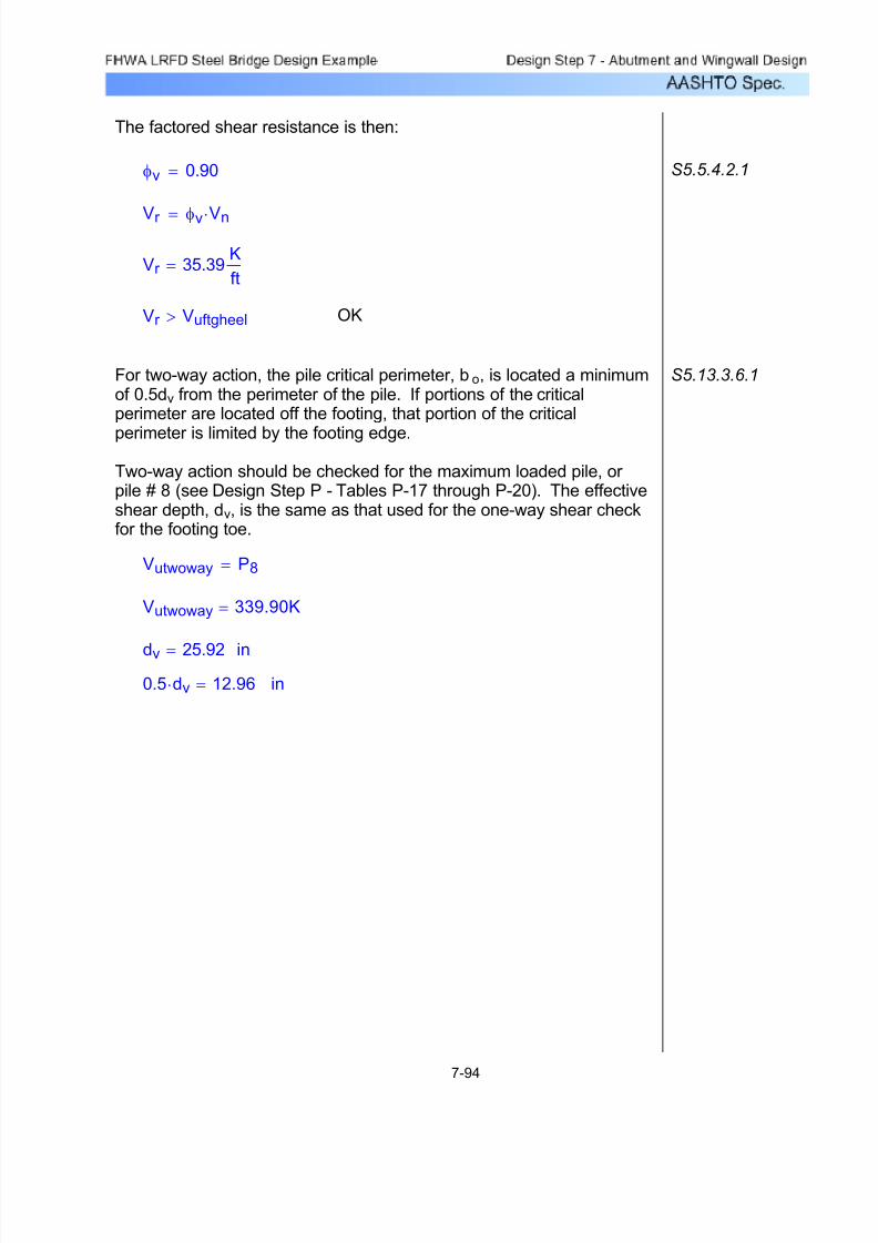
7/29/2019 LRFD steel design.pdf
http://slidepdf.com/reader/full/lrfd-steel-designpdf 437/646
The factored shear resistance is then:
φv 0.90= S5.5.4.2.1
Vr φv Vn⋅=
Vr 35.39K
ft=
Vr Vuftgheel> OK
For two-way action, the pile critical perimeter, bo, is located a minimumof 0.5dv from the perimeter of the pile. If portions of the criticalperimeter are located off the footing, that portion of the critical
perimeter is limited by the footing edge.
Two-way action should be checked for the maximum loaded pile, or pile # 8 (see Design Step P - Tables P-17 through P-20). The effectiveshear depth, dv, is the same as that used for the one-way shear checkfor the footing toe.
S5.13.3.6.1
Vutwoway P8=
Vutwoway 339.90K=
dv 25.92= in
0.5 dv⋅ 12.96= in
7-94

7/29/2019 LRFD steel design.pdf
http://slidepdf.com/reader/full/lrfd-steel-designpdf 438/646
Abutment
footing toe
HP12x53
(Typ.)
Abutment
footing heel
7 8
S t e m
b a c
k f a c e
B a c
k w a
l l b a c
k f a c e
B a c
k w a
l l f r o n
t f a c e
S t e m
f r o n
t f a c e
3 7
. 9 2 i n
.
33.86in.
12.96in.
1 2
. 9 6 i n
.
Pile critical
perimeter
Figure 7-24 Pile Two-way Action Critical Perimeter
In the above figure, it can be seen that the critical perimeter isapproximately at the face of the stem. In fact, the critical perimeter overlaps the front face of the stem by approximately 0.07 inches.Since the overlap is minimal, ignore the overlap and assume thecritical perimeter and the front face of the stem are aligned at thesame plane.
7-95

7/29/2019 LRFD steel design.pdf
http://slidepdf.com/reader/full/lrfd-steel-designpdf 439/646
OKVr Vutwoway>
Vr 843.94K=
Vr φv Vn⋅=
S5.5.4.2.1φv 0.90=
The factored punching shear resistance is then:
Vn 937.71K=use
K0.126 f'c⋅ bo⋅ dv⋅ 937.71=
K0.0630.126
βc
+⎛
⎝
⎞
⎠f'c⋅ bo⋅ dv⋅ 1306.17=
inbo 143.56=
inbo 2 33.86 37.92+( )⋅=
βc 1.12=
ratio of long to short side of critical perimeter βc37.92in
33.86in=
Vn 0.063
0.126
βc+
⎛
⎝
⎞
⎠ f'c⋅ bo⋅ dv⋅ 0.126 f'c⋅ bo⋅ dv⋅≤=
S5.13.3.6.3Two-way action or punching shear resistance for sections withouttransverse reinforcement can then be calculated as follows:
7-96
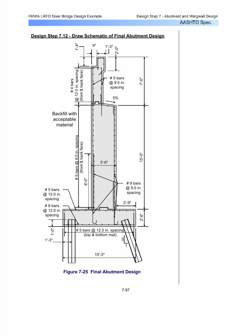
7/29/2019 LRFD steel design.pdf
http://slidepdf.com/reader/full/lrfd-steel-designpdf 440/646
Design Step 7.12 - Draw Schematic of Final Abutment Design
7 ' - 0 "
3'-6"
2 ' - 0 "1'-3"9"
1 ' - 4 "
10'-3"
2 ' - 6 "
5%
1 5 ' - 0 "
# 5 bars @ 12.0 in. spacing
(top & bottom mat)
# 8 bars
@ 12.0 in.
spacing
# 5 bars
@ 12.0 in.
spacing
# 9 bars
@ 9.0 in.
spacing
# 4 b a r s
@ 1
2 . 0
i n .
s p a c
i n g
( f r o n
t & b a c
k f a c e
)
# 5 bars
@ 9.0 in.
spacing
1'-3" 1
' - 0 "
2'-9"
3
1
Backfill with
acceptablematerial
8 ' - 0 " #
5 b a r s
@ 9
. 0 i n
. s p a c
i n g
( f r o n
t & b a c
k f a c e
)
Figure 7-25 Final Abutment Design
7-97
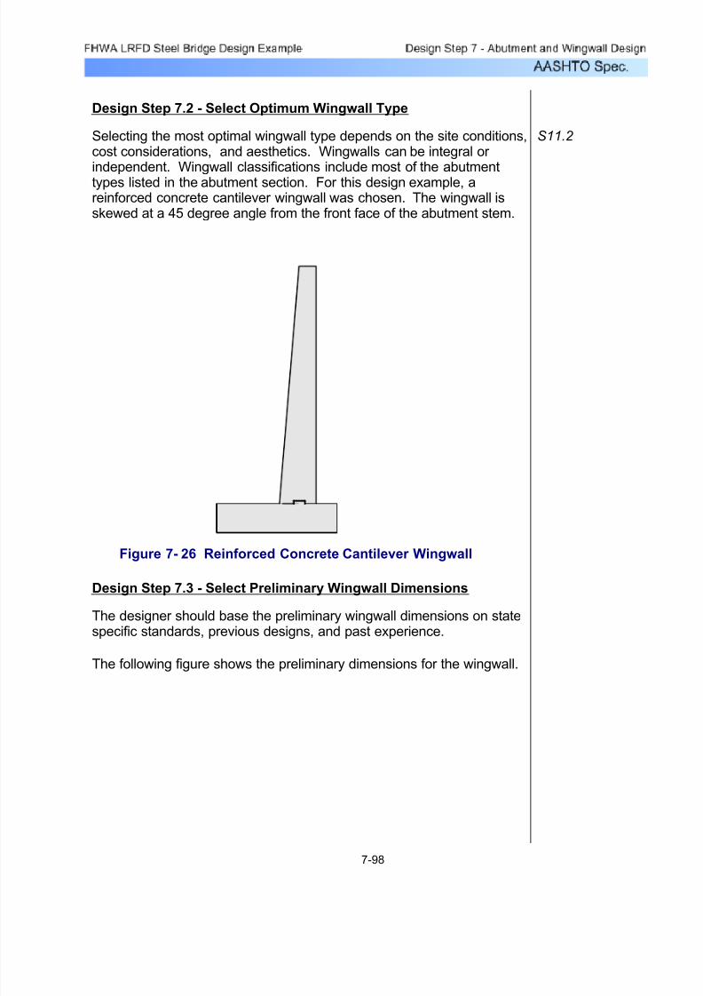
7/29/2019 LRFD steel design.pdf
http://slidepdf.com/reader/full/lrfd-steel-designpdf 441/646
Design Step 7.2 - Select Optimum Wingwall Type
Selecting the most optimal wingwall type depends on the site conditions,cost considerations, and aesthetics. Wingwalls can be integral or independent. Wingwall classifications include most of the abutmenttypes listed in the abutment section. For this design example, areinforced concrete cantilever wingwall was chosen. The wingwall isskewed at a 45 degree angle from the front face of the abutment stem.
S11.2
Figure 7- 26 Reinforced Concrete Cantilever Wingwall
Design Step 7.3 - Select Preliminary Wingwall Dimensions
The designer should base the preliminary wingwall dimensions on statespecific standards, previous designs, and past experience.
The following figure shows the preliminary dimensions for the wingwall.
7-98
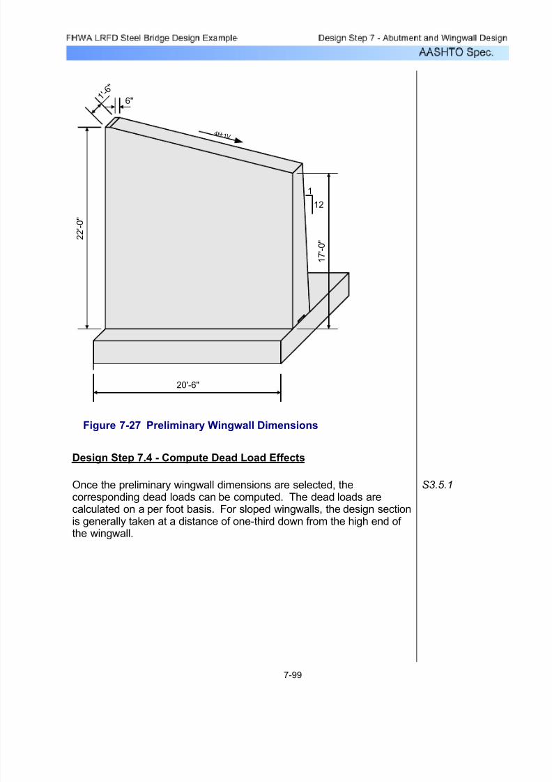
7/29/2019 LRFD steel design.pdf
http://slidepdf.com/reader/full/lrfd-steel-designpdf 442/646
20'-6"
2 2 ' - 0 "
1 ' - 6 "
4 H : 1V
12
1
6"
1 7 ' - 0 "
Figure 7-27 Preliminary Wingwall Dimensions
Design Step 7.4 - Compute Dead Load Effects
Once the preliminary wingwall dimensions are selected, thecorresponding dead loads can be computed. The dead loads arecalculated on a per foot basis. For sloped wingwalls, the design sectionis generally taken at a distance of one-third down from the high end of the wingwall.
S3.5.1
7-99
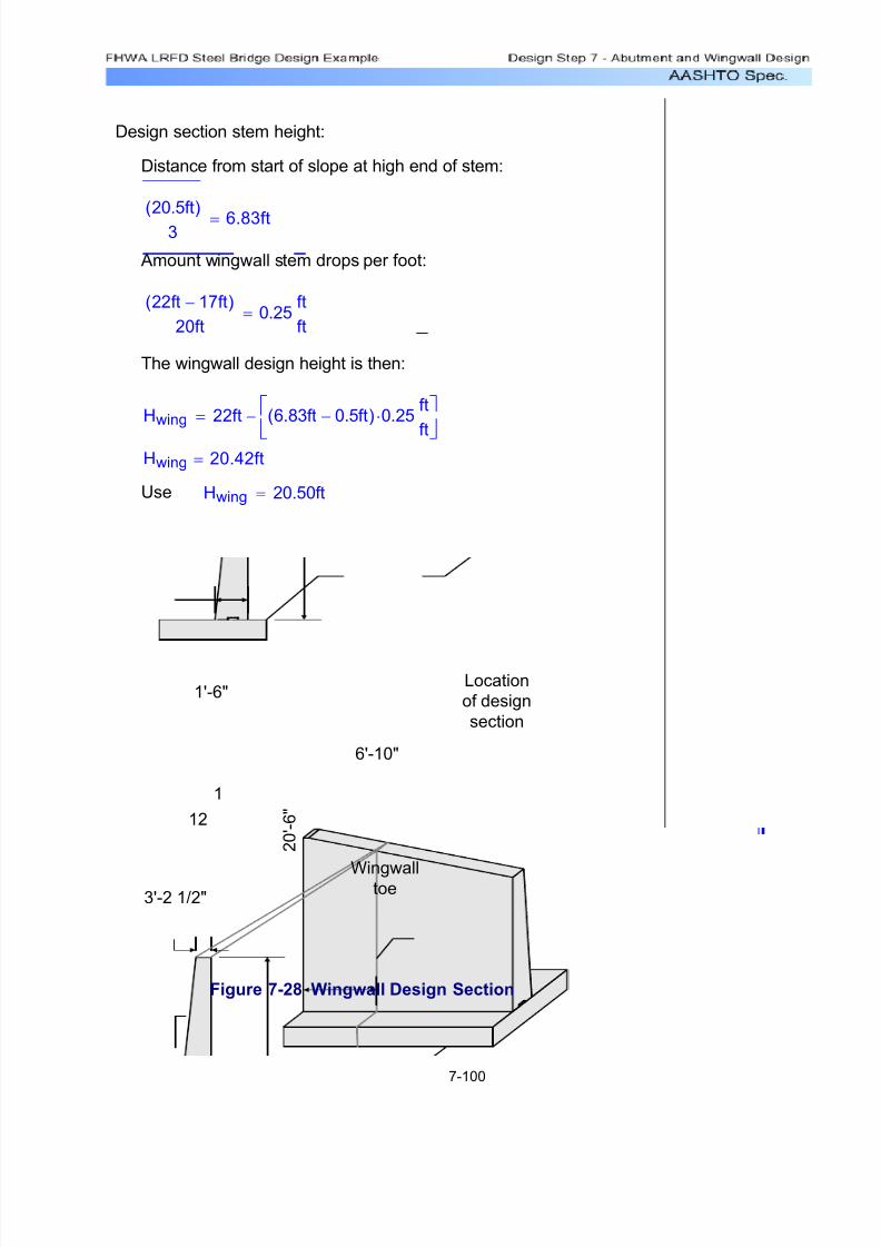
7/29/2019 LRFD steel design.pdf
http://slidepdf.com/reader/full/lrfd-steel-designpdf 443/646
Design section stem height:
Distance from start of slope at high end of stem:
20.5ft( )
3 6.83ft=
Amount wingwall stem drops per foot:
22ft 17ft−( )
20ft0.25
ft
ft=
The wingwall design height is then:
Hwing 22ft 6.83ft 0.5ft−( ) 0.25⋅ft
ft
⎡
⎣
⎤
⎦
−=
Hwing 20.42ft=
Use Hwing 20.50ft=
Wingwalltoe
2 0 ' - 6 "
1
12
3'-2 1/2"
6'-10"
1'-6"Location
of design
section
Figure 7-28 Wingwall Design Section
7-100
7/29/2019 LRFD steel design.pdf
http://slidepdf.com/reader/full/lrfd-steel-designpdf 444/646
S3.11.6
S3.11.5 The earth loads that need to be investigated for this design exampleinclude: loads due to basic lateral earth pressure, loads due touniform surcharge, and live load surcharge loads.
S3.11Earth Loads
This design example assumes that the structure is located inseismic zone I with an acceleration coefficient of 0.02. For seismiczone I, no seismic analysis is required.
S3.10 Earthquake Load
The wind loads acting on the exposed portion of the wingwall front andend elevations are calculated from a base wind pressure of 0.040KSF. In the wingwall final state, the wind loads acting on the wingwallwill only decrease the overturning moment and will be ignored for thisdesign example. For the wingwall temporary state, the wind loads
acting on the wingwall should be investigated. Also, any wind loadsthat produce a transverse shear or moment in the wingwall footing areignored. The reason for this is due to the fact that the majority of forceeffects required to produce a transverse shear or moment will alsoreduce the maximum overturning moment.
S3.8.1.2.3Wind Load on Wingwall
Other load effects that need to be computed include: wind loads,earthquake loads, earth pressure, live load surcharge, and temperatureloads.
Design Step 7.6 - Compute Other Load Effects
Since the wingwall does not support a parapet, the only live load effectsare from live load surcharge. The effects from live load surcharge arecomputed in Design Step 7.6.
Design Step 7.5 - Compute Live Load Effects
DLwwstem 7.24K
ft=
DLwwstem1.5ft 3.21ft+
2
⎛ ⎝
⎞ ⎠
20.50⋅ ft⎡⎣
⎤⎦
Wc⋅=
Wingwall stem:
7-101

7/29/2019 LRFD steel design.pdf
http://slidepdf.com/reader/full/lrfd-steel-designpdf 445/646
Figure 7-29 Wingwall Stem Design Earth Pressure
Wingwall
toe
2 0 ' - 6 "
1
12
3'-2 1/2"
1'-6"
18.5°
18.5°
Horizontal earth
load, REHstem
p
7 ' - 6 "
2 2 ' - 6 "
p 0.81ksf =
p ka γs⋅ z⋅=
Depth below the surface of the earthz 20.5ft 2.0ft+=
STable 3.5.1-1use average of loose and compacted gravelγs 0.120kcf =
obtained from geotechnical informationka 0.3=
Bottom of wingwall stem lateral earth load:
p ka γs⋅ z⋅=
S3.11.5.1To obtain the lateral loads due to basic earth pressure, the earthpressure (p) must first be calculated from the following equation.
S3.11.5 Loads due to basic lateral earth pressure:
7-102

7/29/2019 LRFD steel design.pdf
http://slidepdf.com/reader/full/lrfd-steel-designpdf 446/646
∆p k γs⋅ heq⋅=
Loads due to live load surcharge must be applied when a vehicular live load acts on the backfill surface behind the backface withinone-half the wall height. Since the distance from the wingwall backface to the edge of traffic is greater than one foot, the equivalent
height of fill is constant. The horizontal pressure increase due to liveload surcharge is estimated based on the following equation:
S3.11.6.4Loads due to live load surcharge:
Since an approach slab and roadway will cover the abutment backfillmaterial, no uniform surcharge load will be applied.
S3.11.6.1Loads due to uniform surcharge:
REHstemvert 2.89K
ft=
REHstemvert REHstem sin 18.5deg( )⋅=
REHstemhoriz 8.64K
ft=
REHstemhoriz REHstem cos 18.5deg( )⋅=
Since the ground line is sloped, REHstem, must be broken downinto horizontal and vertical components as follows:
REHstem 9.11K
ft=
REHstem1
2
⎛ ⎝
⎞ ⎠
p⋅ hwwstem⋅=
hwwstem 20.5ft 2.0ft+=
SC3.11.5.1
S3.11.5.1
Once the lateral earth pressure is calculated, the lateral loaddue to the earth pressure can be calculated. This load actsat a distance of H/3 from the bottom of the section beinginvestigated. For cases where the ground line is sloped, H
is taken as the height from the top of earth to the bottom of the section being investigated.
7-103

7/29/2019 LRFD steel design.pdf
http://slidepdf.com/reader/full/lrfd-steel-designpdf 447/646
There are two critical locations where the force effects need tobe combined and analyzed for design. They include: the bottomof stem or top of footing and the bottom of footing. For the stemdesign, transverse horizontal loads do not need be considereddue to the high moment of inertia about that axis, but at thebottom of footing, the transverse horizontal loads will need to beconsidered for the footing and pile design. Note that the footingdesign calculations for wingwalls are similar to abutments.Therefore, the wingwall footing design calculations will not beshown.
Design Step 7.7 - Analyze and Combine Force Effects
Temperature loads are not applicable for the wingwall design.
S3.12 Loads due to temperature:
RLSstemvert 0.51K
ft=
RLSstemvert RLSstem sin 18.5deg( )⋅=
RLSstemhoriz 1.54K
ft=
RLSstemhoriz RLSstem cos 18.5deg( )⋅=
Since the ground line is sloped, RLSstem, must be broken downinto horizontal and vertical components as follows:
RLSstem 1.62K
ft=
RLSstem ∆p hwwstem⋅=
The lateral load due to the live load surcharge is:
∆p 0.072ksf =
∆p k γs⋅ heq⋅=
STable 3.11.6.4-1equivalent height of soil for vehicular loadingheq 2.0ft=
STable 3.5.1-1use average of loose and compacted gravelγs 0.120kcf =
k ka=
Bottom of wingwall stem live load surcharge load:
7-104

7/29/2019 LRFD steel design.pdf
http://slidepdf.com/reader/full/lrfd-steel-designpdf 448/646
Bottom of Wingwall Stem
The combination of force effects for the bottom of the wingwallstem includes:
Figure 7-30 Wingwall Stem Dimensions and Loading
7-105

7/29/2019 LRFD steel design.pdf
http://slidepdf.com/reader/full/lrfd-steel-designpdf 449/646
FvstmstrI 9.05K
ft=
FvstmstrI γDC DLwwstem⋅=The factored vertical force at the base of the wingwall stem is:
STable 3.4.1-1γLS 1.75=
STable 3.4.1-2 γEH 1.50=
STable 3.4.1-2 γDC 1.25=
The following load factors will be used to calculate thecontrolling force effects for Strength I:
Wingwall stem Strength I force effects:
RLSstemhoriz 1.54K
ft=
REHstemhoriz 8.64K
ft=
DLwwstem 7.24K
ft=
The loads that are required to combine force effects at the base of thewingwall stem include:
Table 7-7 Applicable Wingwall Stem Limit States with the
Corresponding Load Factors
STable 3.4.1-2
STable 3.4.1-1
Load γmax γmin γmax γmin γmax γmin γmax γmin
DC 1.25 0.90 1.25 0.90 1.25 0.90 1.00 1.00
EH 1.50 0.90 1.50 0.90 1.50 0.90 1.00 1.00
LS 1.75 1.75 --- --- 1.35 1.35 1.00 1.00
Load Factors
Strength I Strength III Strength V Service I
The force effects for the wingwall stem will be combined for thefollowing limit states.
7-106
7/29/2019 LRFD steel design.pdf
http://slidepdf.com/reader/full/lrfd-steel-designpdf 450/646
VustmstrIII 12.96K
ft=
VustmstrIII γEH REHstemhoriz⋅=
The factored longitudinal shear force at the base of the abutment stem
is:
FvstmstrIII 9.05K
ft=
FvstmstrIII γDC DLwwstem⋅=
The factored vertical force at the base of the wingwall stem is:
STable 3.4.1-2 γEH 1.50=
STable 3.4.1-2 γDC 1.25=
The following load factors will be used to calculate the forceeffects for Strength III:
Wingwall stem Strength III force effects:
MustmstrI 127.46K ft⋅ft
=
MustmstrI γEH REHstemhoriz⋅ 7.5⋅ ft⋅( )γLS RLSstemhoriz⋅ 11.25⋅ ft⋅( )+
...=
The factored moment about the bridge transverse axis at the baseof the wingwall stem is:
VustmstrI 15.65K
ft=
VustmstrI γEH REHstemhoriz⋅( ) γLS RLSstemhoriz⋅( )+=
The factored longitudinal shear force at the base of the wingwallstem is:
7-107

7/29/2019 LRFD steel design.pdf
http://slidepdf.com/reader/full/lrfd-steel-designpdf 451/646
MustmstrV 120.55K ft⋅ft
=
MustmstrV γEH REHstemhoriz⋅ 7.5⋅ ft⋅( )γLS RLSstemhoriz⋅ 11.25⋅ ft⋅( )+
...=
The factored longitudinal moment at the base of the wingwallstem is:
VustmstrV 15.04K
ft=
VustmstrV γEH REHstemhoriz⋅( ) γLS RLSstemhoriz⋅( )+=
The factored longitudinal shear force at the base of the wingwallstem is:
FvstmstrV 9.05K
ft=
FvstmstrV γDC DLwwstem⋅=
The factored vertical force at the base of the wingwall stem is:
STable 3.4.1-1γLS 1.35=
STable 3.4.1-2 γEH 1.50=
STable 3.4.1-2 γDC 1.25=
The following load factors will be used to calculate the forceeffects for Strength V:
Wingwall stem Strength V force effects:
MustmstrIII 97.22K ft⋅ft
=
MustmstrIII γEH REHstemhoriz⋅ 7.5⋅ ft⋅=
The factored longitudinal moment at the base of the wingwallstem is:
7-108

7/29/2019 LRFD steel design.pdf
http://slidepdf.com/reader/full/lrfd-steel-designpdf 452/646
MustmservI 82.10K ft⋅ft
=
MustmservI γEH REHstemhoriz⋅ 7.5⋅ ft⋅( )γLS RLSstemhoriz⋅ 11.25⋅ ft⋅( )+
...=
The factored longitudinal moment at the base of thewingwall stem is:
VustmservI 10.18K
ft=
VustmservI γEH REHstemhoriz⋅( ) γLS RLSstemhoriz⋅( )+=
The factored longitudinal shear force at the base of the wingwall stemis:
FvstmservI 7.24K
ft=
FvstmservI γDC DLwwstem⋅=
The factored vertical force at the base of the wingwall stem is:
STable 3.4.1-1γLS 1.00=
STable 3.4.1-2 γEH 1.00=
STable 3.4.1-2 γDC 1.00=
The following load factors will be used to calculate the forceeffects for Service I:
Wingwall stem Service I force effects:
7-109

7/29/2019 LRFD steel design.pdf
http://slidepdf.com/reader/full/lrfd-steel-designpdf 453/646
The maximum factored wingwall stem vertical force, shear force,and moment for the strength limit state are:
Fvertstemmax max FvstmstrI FvstmstrIII, FvstmstrV,( )=
Fvertstemmax 9.05K
ft=
Vuwwstemmax max VustmstrI VustmstrIII, VustmstrV,( )=
Vuwwstemmax 15.65K
ft=
Muwwstemmax max MustmstrI MustmstrIII, MustmstrV,( )=
Muwwstemmax 127.46K ft⋅ft
=
7-110

7/29/2019 LRFD steel design.pdf
http://slidepdf.com/reader/full/lrfd-steel-designpdf 454/646
Design Step 7.9 - Design Wingwall Stem
Design for flexure:
Assume #9 bars:
bar_diam 1.128in=
bar_area 1.00in2=
First, the minimum reinforcement requirements will be calculated. Thetensile reinforcement provided must be enough to develop a factoredflexural resistance at least equal to the lesser of 1.2 times the crackingstrength or 1.33 times the factored moment from the applicablestrength load combinations.
S5.7.3.3.2
The cracking strength is calculated by:
SEquation
5.7.3.6.2-2 Mcr f r Ig⋅
yt=
Centroidal
Axis
Front face of
wingwall at
base
#9 bars
@ 9.0 in.
spacing
3 ' - 2 1 / 2 "
3 1 / 1 6 "
1 ' - 7 1 / 4 "
1'-0"
Figure 7-31 Wingwall Cracking Moment Dimensions
7-111

7/29/2019 LRFD steel design.pdf
http://slidepdf.com/reader/full/lrfd-steel-designpdf 455/646

7/29/2019 LRFD steel design.pdf
http://slidepdf.com/reader/full/lrfd-steel-designpdf 456/646
As 1.33in2
= per foot
Once the bar size and spacing are known, the maximum reinforcement
limit must be checked.
S5.7.3.3.1
T As f y⋅= T 80.00K=
aT
0.85 f'c⋅ b⋅= a 1.96 in=
β1 0.85= S5.7.2.2
ca
β1
= c 2.31in= S5.7.2.2
c
de0.07= where
c
de0.42≤ S5.7.3.3.1
0.07 0.42≤ OK
Solve for the required amount of reinforcing steel, as follows:
φf 0.90= S5.5.4.2.1
b 12in=
f'c 4.0ksi=
f y 60ksi=
RnMuwwstemdes 12⋅ in
φf b⋅ de2⋅( )
= Rn 0.13ksi=
ρ 0.85f'c
f y
⎛
⎝
⎞
⎠1.0 1.0
2 Rn⋅( )
0.85 f'c⋅( )−−
⎡⎣
⎤⎦
⋅= ρ 0.00214=
Note: The above two equations are derived formulas that can be foundin most reinforced concrete textbooks.
As ρb
ft⋅ de⋅= As 0.91
in2
ft=
bar_area
As13.2in=Required bar spacing =
Use #9 bars @ bar_space 9.0in= to match the abutmentstem vertical bar spacing
As bar_area12in
bar_space
⎛ ⎝
⎞ ⎠
⋅=
7-113

7/29/2019 LRFD steel design.pdf
http://slidepdf.com/reader/full/lrfd-steel-designpdf 457/646
n 8=Use
n 7.97=nEs
Ec=
S5.4.2.4Ec 3640ksi=
S5.4.3.2 Es 29000ksi=
f sa 26.48ksi=Use
0.6f y 36.00ksi=f sa 26.48ksi=
f sa 0.6 f y⋅≤wheref saZ
dc Ac⋅( )
1
3
=
The equation that gives the allowable reinforcement service load stressfor crack control is:
Ac 46.15in2
=
Ac 2 dc( )⋅ bar_space⋅=
Concrete area with centroid the same astransverse bar and bounded by the crosssection and line parallel to neutral axis:
dc 2.56in=dc 2.0in
bar_diam
2+=use
dc 3.06in=
dc 2.5inbar_diam
2+=
Thickness of clear cover used to compute dc should not be greater than 2 inches:
Z 130K
in=Since this design example assumes that
the wingwall will be exposed to deicingsalts, use:
S5.7.3.4The control of cracking by distribution of reinforcement must bechecked.
Check crack control:
7-114
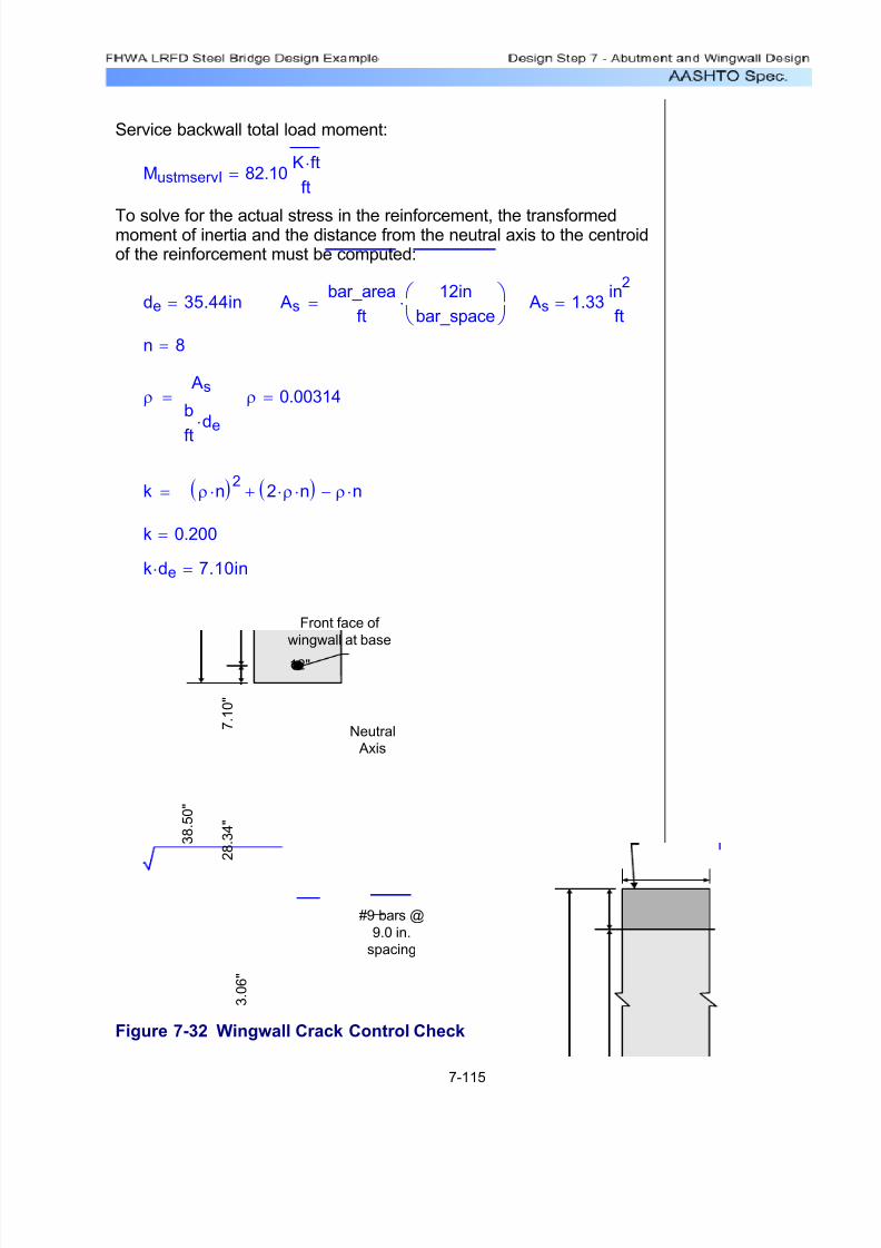
7/29/2019 LRFD steel design.pdf
http://slidepdf.com/reader/full/lrfd-steel-designpdf 458/646
Service backwall total load moment:
MustmservI 82.10K ft⋅ft
=
To solve for the actual stress in the reinforcement, the transformedmoment of inertia and the distance from the neutral axis to the centroidof the reinforcement must be computed:
de 35.44in= Asbar_area
ft
12in
bar_space
⎛ ⎝
⎞ ⎠
⋅= As 1.33in
2
ft=
n 8=
ρ As
b
ft
de⋅= ρ 0.00314=
k ρ n⋅( )22 ρ⋅ n⋅( )+ ρ n⋅−=
k 0.200=
k de⋅ 7.10in=
Neutral
Axis
Front face of
wingwall at base
#9 bars @
9.0 in.
spacing
7 . 1
0 "
2 8
. 3 4 "
3 8
. 5 0 "
12"
3 . 0
6 "
Figure 7-32 Wingwall Crack Control Check
7-115
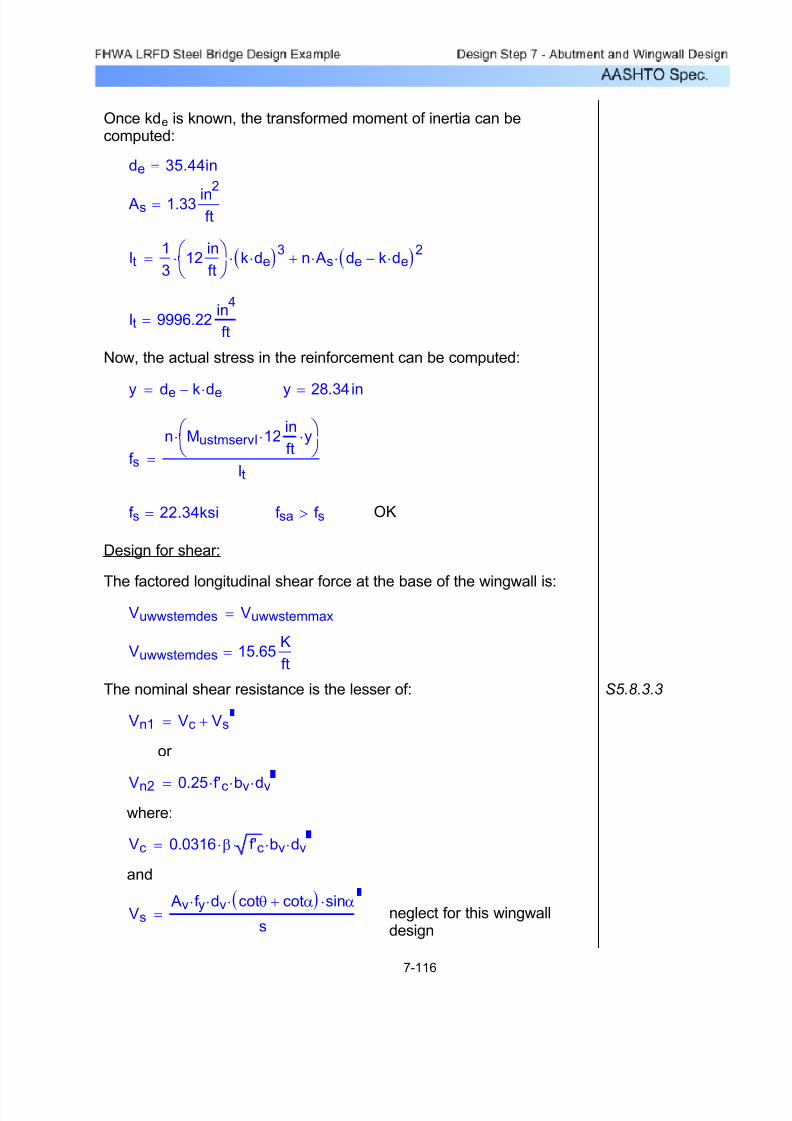
7/29/2019 LRFD steel design.pdf
http://slidepdf.com/reader/full/lrfd-steel-designpdf 459/646
neglect for this wingwalldesign
Vs Av f y⋅ dv⋅ cotθ cotα+( )⋅ sinα⋅
s=
and
Vc 0.0316 β⋅ f'c⋅ bv⋅ dv⋅=
where:
Vn2 0.25 f'c⋅ bv⋅ dv⋅=
or
Vn1 Vc Vs+=
S5.8.3.3The nominal shear resistance is the lesser of:
Vuwwstemdes 15.65K
ft=
Vuwwstemdes Vuwwstemmax=The factored longitudinal shear force at the base of the wingwall is:
Design for shear:
OKf sa f s>f s 22.34ksi=
f s
n MustmservI 12⋅in
fty⋅⎛
⎝ ⎞ ⎠
⋅
It=
y 28.34 in=y de k de⋅−=
Now, the actual stress in the reinforcement can be computed:
It 9996.22in
4
ft=
It1
312
in
ft
⎛ ⎝
⎞ ⎠
⋅ k de⋅( )3⋅ n As⋅ de k de⋅−( )2
⋅+=
As 1.33 in2
ft=
de 35.44in=
Once kde is known, the transformed moment of inertia can becomputed:
7-116

7/29/2019 LRFD steel design.pdf
http://slidepdf.com/reader/full/lrfd-steel-designpdf 460/646
f'c 4.0= ksi
Vn1 0.0316 β⋅ f'c⋅ bv⋅ dv⋅=
Vn1 52.27=
K
ft
Vn2 0.25 f'c⋅ bv⋅ dv⋅=
Vn2 413.52=K
ft
Use: Vn 52.27K
ft=
The factored shear resistance is then:
φv 0.90= S5.5.4.2.1
Vr φv Vn⋅=
Vr 47.04K
ft=
Vr Vuwwstemdes> OK
Before the nominal shear resistance can be calculated, all thevariables used in the above equations need to be defined.
β 2.0= S5.8.3.4.1
bv 12= in
dv max dea
2− 0.9 de⋅, 0.72 h⋅,⎛
⎝ ⎞ ⎠
= S5.8.2.9
where:
de 35.44in=
a 1.96in=
h 38.50= in
Therefore:
dv 34.46= in
Now, Vn1 and Vn2 can be calculated:
For
7-117
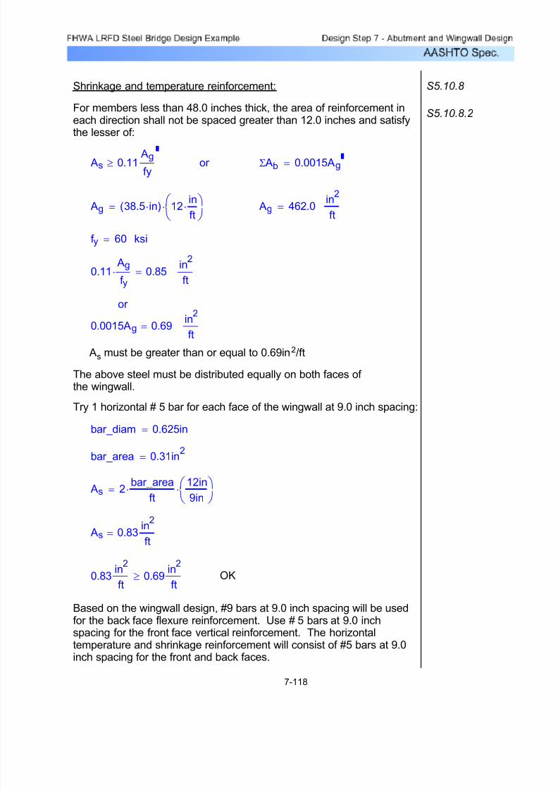
7/29/2019 LRFD steel design.pdf
http://slidepdf.com/reader/full/lrfd-steel-designpdf 461/646
Based on the wingwall design, #9 bars at 9.0 inch spacing will be usedfor the back face flexure reinforcement. Use # 5 bars at 9.0 inchspacing for the front face vertical reinforcement. The horizontaltemperature and shrinkage reinforcement will consist of #5 bars at 9.0inch spacing for the front and back faces.
OK0.83in
2
ft0.69
in2
ft≥
As 0.83in
2
ft=
As 2bar_area
ft⋅
12in
9in
⎛ ⎝
⎞ ⎠
⋅=
bar_area 0.31in2
=
bar_diam 0.625in=
Try 1 horizontal # 5 bar for each face of the wingwall at 9.0 inch spacing:
The above steel must be distributed equally on both faces of the wingwall.
As must be greater than or equal to 0.69in2/ft
in2
ft0.0015Ag 0.69=
or
in2
ft0.11
Ag
f y⋅ 0.85=
ksif y 60=
in2
ft Ag 462.0= Ag 38.5 in⋅( ) 12
in
ft⋅⎛
⎝ ⎞ ⎠
⋅=
Σ Ab 0.0015Ag=or As 0.11 Ag
fy≥
S5.10.8.2 For members less than 48.0 inches thick, the area of reinforcement ineach direction shall not be spaced greater than 12.0 inches and satisfythe lesser of:
S5.10.8 Shrinkage and temperature reinforcement:
7-118

7/29/2019 LRFD steel design.pdf
http://slidepdf.com/reader/full/lrfd-steel-designpdf 462/646
Design Step 7.12 - Draw Schematic of Final Wingwall Design
2 0 ' - 6 "
3'-2 1/2"
1'-6"
2 1/2" (Typ.)
# 5
b a r s
@ 9
. 0 i n
. s p a c
i n g
( f r o n
t &
b a c
k f a c
e )
#9 bars @
9.0 in.spacing
1
12
#5 bars @
9.0 in.
spacing
Backfill with
acceptable material
8 ' - 0 "
Figure 7-33 Final Wingwall Design
7-119
7/29/2019 LRFD steel design.pdf
http://slidepdf.com/reader/full/lrfd-steel-designpdf 463/646
69Design Step 8.12 - Final Pier Schematic
62Design Step 8.11 - Design Pier Footing
61Design Step 8.10 - Design Pier Piles
51Design Step 8.9 - Design Pier Column
39Design Step 8.8 - Design Pier Cap
24Design Step 8.7 - Analyze and Combine Force Effects
10Design Step 8.6 - Compute Other Load Effects
8Design Step 8.5 - Compute Live Load Effects
6Design Step 8.4 - Compute Dead Load Effects
5Design Step 8.3 - Select Preliminary Pier Dimensions
4Design Step 8.2 - Select Optimum Pier Type
2Design Step 8.1 - Obtain Design Criteria
Page
Table of Contents
Pier Design ExampleDesign Step 8
8-1

7/29/2019 LRFD steel design.pdf
http://slidepdf.com/reader/full/lrfd-steel-designpdf 464/646
C5.4.2.1
Concrete 28-day compressive strength - For all components of thispier design example, 4.0 ksi is used for the 28-day compressivestrength. However, per the Specifications, 2.4 ksi could be used for thepier footing.
S5.4.3f y 60.0ksi=Reinforcementstrength:
S5.4.2.1
CTable5.4.2.1-1f'c 4.0ksi=Concrete 28-day
compressive strength:
STable 3.5.1-1Wc 0.150kcf =Concrete density:
Material Properties:
klf K
ft=ksf
K
ft2
=ksiK
in2
=kcf K
ft3
=K 1000lb=
The following units are defined for use in this design example:
Refer to Design Step 1 for introductory information about this designexample. Additional information is presented about the design
assumptions, methodology, and criteria for the entire bridge, includingthe pier.
This pier design example is based on AASHTO LRFD Bridge Design
Specifications (through 2002 interims). The design methods presentedthroughout the example are meant to be the most widely used ingeneral bridge engineering practice.
The first design step is to identify the appropriate design criteria. Thisincludes, but is not limited to, defining material properties, identifyingrelevant superstructure information, determining the required pier height, and determining the bottom of footing elevation.
Design Step 8.1 - Obtain Design Criteria
8-2

7/29/2019 LRFD steel design.pdf
http://slidepdf.com/reader/full/lrfd-steel-designpdf 465/646
Number of girders: N 5=
Deck overhang: DOH 3.9375ft=
Span length: Lspan 120.0ft=
Parapet height: Hpar 3.5ft=
Deck overhangthickness: to 9.0in=
Haunch thickness: Hhnch 3.5in= (includes top flange)
Web depth: Do 66.0in=
Bot. flange thickness: tbf 2.25in= (maximum thickness)
Bearing height: Hbrng 5.0in=
Superstructure Depth: Hsuper Hpar to Hhnch+ Do+ tbf +
12in
ft
⎛
⎝
⎞
⎠
+=
Hsuper 10.23ft=
Reinforcing steel cover requirements (assume non-epoxy rebars):
Pier cap: Cover cp 2.5in= STable 5.12.3-1
Pier column: Cover co 2.5in= STable 5.12.3-1
Footing top cover: Cover ft 2.0in= STable 5.12.3-1
Footing bottom cover: Cover fb 3.0in= STable 5.12.3-1
Pier cap and column cover - Since no joint exists in the deck at the
pier, a 2-inch cover could be used with the assumption that the pier isnot subject to deicing salts. However, it is assumed here that the pier can be subjected to a deicing salt spray from nearby vehicles.Therefore, the cover is set at 2.5 inches.
STable 5.12.3-1
Footing top cover - The footing top cover is set at 2.0 inches. STable 5.12.3-1Footing bottom cover - Since the footing bottom is cast directly
against the earth, the footing bottom cover is set at 3.0 inches.
STable 5.12.3-1
Relevant superstructure data:
Girder spacing: S 9.75ft=
8-3

7/29/2019 LRFD steel design.pdf
http://slidepdf.com/reader/full/lrfd-steel-designpdf 466/646
Superstructure data - The above superstructure data is important
because it sets the width of the pier cap and defines the depth andlength of the superstructure needed for computation of wind loads.
S3.8
Pier height - Guidance on determining the appropriate pier height
can be found in the AASHTO publication A Policy on Geometric
Design of Highways and Streets. It will be assumed here thatadequate vertical clearance is provided given a ground line that istwo feet above the top of the footing and the pier dimensions given inDesign Step 8.3.
S2.3.3.2
Bottom of Footing Elevation - The bottom of footing elevation may
depend on the potential for scour (not applicable in this example) and/or the geotechnical properties of the soil and/or rock. However, as aminimum, it should be at or below the frost depth for a given geographicregion. In this example, it is assumed that the two feet of soil above the
footing plus the footing thickness provides sufficient depth below theground line for frost protection of the structure.
S10.6.1.2
Design Step 8.2 - Select Optimum Pier Type
Selecting the most optimal pier type depends on site conditions, costconsiderations, superstructure geometry, and aesthetics. The mostcommon pier types are single column (i.e., "hammerhead"), solid walltype, and bent type (multi-column or pile bent). For this designexample, a single column (hammerhead) pier was chosen. A typicalhammerhead pier is shown in Figure 8-1.
S11.2
Figure 8-1 Typical Hammerhead Pier
8-4
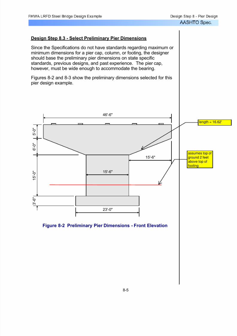
7/29/2019 LRFD steel design.pdf
http://slidepdf.com/reader/full/lrfd-steel-designpdf 467/646
Design Step 8.3 - Select Preliminary Pier Dimensions
Since the Specifications do not have standards regarding maximum or minimum dimensions for a pier cap, column, or footing, the designer
should base the preliminary pier dimensions on state specificstandards, previous designs, and past experience. The pier cap,however, must be wide enough to accommodate the bearing.
Figures 8-2 and 8-3 show the preliminary dimensions selected for thispier design example.
5 ' - 0 "
6 ' - 0 "
1 5 ' - 0 " 15'-6"
46'-6"
3 ' - 6 "
23'-0"
15'-6"
Figure 8-2 Preliminary Pier Dimensions - Front Elevation
8-5
assumes top of
ground 2 feetabove top of
footing
length = 16.62'

7/29/2019 LRFD steel design.pdf
http://slidepdf.com/reader/full/lrfd-steel-designpdf 468/646
5 ' - 0 "
6 ' - 0 "
5'-0"
12'-0"
4'-6"
Figure 8-3 Preliminary Pier Dimensions - End Elevation
Design Step 8.4 - Compute Dead Load Effects
Once the preliminary pier dimensions are selected, the correspondingdead loads can be computed. The pier dead loads must then becombined with the superstructure dead loads. The superstructure deadloads shown below are obtained from the superstructureanalysis/design software. Based on the properties defined in DesignStep 3 (Steel Girder Design), any number of commercially availablesoftware programs can be used to obtain these loads. For this designexample, the AASHTO Opis software was used, and the values shownbelow correspond to the first design iteration.
S3.5.1
Exterior girder dead load reactions (DC and DW):
RDCE 253.70K= RDWE 39.20K=
Interior girder dead load reactions (DC and DW):
RDCI 269.10K= RDWI 39.20K=
8-6

7/29/2019 LRFD steel design.pdf
http://slidepdf.com/reader/full/lrfd-steel-designpdf 469/646
EVftg 49.50K=
EVftg 0.120kcf 2ft( )⋅ 23ft 12⋅ ft 15.5ft 4.5⋅ ft−( )⋅=
STable 3.5.1-1
In addition to the above dead loads, the weight of the soil on top of thefooting must be computed. The two-foot height of soil above the footingwas previously defined. Assuming a unit weight of soil at 0.120 kcf :
DLftg
144.90K=
DLftg 3.5ft 23⋅ ft 12⋅ ft( )Wc=
Pier footing dead load:
DLcol 156.94K=
DLcol 15.5ft 4.5⋅ ft 15⋅ ft( ) Wc⋅=
Pier column dead load:
DLcap 313.88K=
DLcap 2 DLovrhg⋅ DLint+=Total:
DLint 127.88K=
DLint 11ft 5⋅ ft 15.5⋅ ft( ) Wc⋅=Interior:
DLovrhg 93.00K=
DLovrhg 5ft 5⋅ ft 15.5⋅ ft( ) Wc⋅1
26ft 5⋅ ft 15.5⋅ ft( )⋅ Wc⋅+=Overhang:
Pier cap dead load:
8-7

7/29/2019 LRFD steel design.pdf
http://slidepdf.com/reader/full/lrfd-steel-designpdf 470/646
Design Step 8.5 - Compute Live Load Effects
For the pier in this design example, the maximum live load effects in thepier cap, column and footing are based on either one, two or three
lanes loaded (whichever results in the worst force effect). Figure 8-4illustrates the lane positions when three lanes are loaded.
The positioning shown in Figure 8-4 is arrived at by first determining thenumber of design lanes, which is the integer part of the ratio of the clear roadway width divided by 12 feet per lane. Then the lane loading,which occupies ten feet of the lane, and the HL-93 truck loading, whichhas a six-foot wheel spacing and a two-foot clearance to the edge of the lane, are positioned within each lane to maximize the force effectsin each of the respective pier components.
S3.6.1.1.1
S3.6.1.2.1
S3.6.1.2.4
S3.6.1.3.1
12'-0” Lane - C
44'-0"
2'-0"
6'-0"
2'-0"
12'-0” Lane - B
2'-0"
6'-0"
2'-0"
12'-0” Lane - A
2'-0"
6'-0"
2'-0"
9'-9"9'-9"9'-9"9'-9" 2'-6"
L Pier C
1 2 3 4 5
w
PP
ww
PP PP
2'-0"
Figure 8-4 Pier Live Loading
8-8

7/29/2019 LRFD steel design.pdf
http://slidepdf.com/reader/full/lrfd-steel-designpdf 471/646
R5_cPwheel 4.25ft 10.25ft+( )⋅ Wlane 10⋅ ft 7.25⋅ ft+
9.75ft=
The next step is to compute the reactions due to the above loads ateach of the five bearing locations. This is generally carried out byassuming the deck is pinned (i.e., discontinuous) at the interior
girder locations but continuous over the exterior girders. Solving for the reactions is then elementary. The computations for the reactionswith only Lane C loaded are illustrated below as an example. Thesubscripts indicate the bearing location and the lane loaded toobtain the respective reaction:
Wlane 8.77K
ft=Wlane
Rlane
10ft0.90( )⋅=
S3.6.2.1
The value of the unfactored uniformly distributed load whichrepresents the girder lane load reaction in Figure 8-4 is computednext. This load is transversely distributed over ten feet and is notsubject to dynamic load allowance.
Pwheel 74.51K=
PwheelRtruck
21 IM+( )⋅ 0.90( )⋅=
The values of the unfactored concentrated loads which representthe girder truck load reaction per wheel line in Figure 8-4 are:
STable 3.6.2.1-1IM 0.33=Dynamic load allowance, IM
Rlane 97.40K=
Rtruck 124.50K=
S3.6.1.3.1
The unfactored girder reactions for lane load and truck load areobtained from the superstructure analysis/design software. Thesereactions do not include dynamic load allowance and are given on aper lane basis (i.e., distribution factor = 1.0). Also, the reactions do not
include the ten percent reduction permitted by the Specifications for interior pier reactions that result from longitudinally loading thesuperstructure with a truck pair in conjunction with lane loading. Thevalue of these reactions from the first design iteration are as follows:
8-9
7/29/2019 LRFD steel design.pdf
http://slidepdf.com/reader/full/lrfd-steel-designpdf 472/646
S3.6.2.1
S3.6.1.1.1The total braking force is computed based on the number of designlanes in the same direction. It is assumed in this example that thisbridge is likely to become one-directional in the future. Therefore,any and all design lanes may be used to compute the governingbraking force. Also, braking forces are not increased for dynamicload allowance. The calculation of the braking force for a singletraffic lane follows:
5 percent of the axle weights of the design tandem plus lane load
5 percent of the axle weights of the design truck plus lane load
25 percent of the axle weights of the design truck or tandem
The braking force per lane is the greater of:
Since expansion bearings exist at the abutments, the entire longitudinalbraking force is resisted by the pier.
S3.6.4Braking Force
Other load effects that will be considered for this pier design includebraking force, wind loads, temperature loads, and earthquake loads.
Design Step 8.6 - Compute Other Load Effects
R1_c 0.0K=R1_b 0.0K=R1_a 4.19K=
R2_c 0.0K=R2_b 0.0K=R2_a 161.59K=
R3_c 0.0K=R3_b 118.36K=R3_a 70.96K=
R4_b 118.36K=R4_a 0.0K=
R5_b 0.0K=R5_a 0.0K=
The reactions at bearings 1, 2 and 3 with only Lane C loaded are zero.Calculations similar to those above yield the following live load reactionswith the remaining lanes loaded (for simplicity, it is assumed that LaneB's loading is resisted entirely, and equally, by bearings 3 and 4):
R4_c 60.69K=
R4_c Pwheel 2⋅ Wlane 10⋅ ft+ R5_c−=
R5_c 176.00K=
8-10

7/29/2019 LRFD steel design.pdf
http://slidepdf.com/reader/full/lrfd-steel-designpdf 473/646
BRKbrgBRK
5=
S3.6.4The Specifications state that the braking force is applied at adistance of six feet above the roadway surface. However, since the
bearings are assumed incapable of transmitting longitudinal moment,the braking force will be applied at the bearing elevation (i.e., fiveinches above the top of the pier cap). This force may be applied ineither horizontal direction (back or ahead station) to cause themaximum force effects. Additionally, the total braking force istypically assumed equally distributed among the bearings:
BRK 18.00 K=
BRK max BRKtrk BRKtan, BRKtrk_lan, BRKtan_lan,( )=Use
BRKtan_lan 10.18K=
BRKtan_lan 0.05 25K 25K+( ) 0.64K
ft 240⋅ ft⎛ ⎝ ⎞ ⎠+⎡⎣ ⎤⎦⋅=
5 percent of the axle weights of the design tandem plus lane load:
BRKtrk_lan 11.28K=
BRKtrk_lan 0.05 32K 32K+ 8K+( ) 0.64K
ft240⋅ ft⎛
⎝ ⎞ ⎠
+⎡⎣
⎤⎦
⋅=
5 percent of the axle weights of the design truck plus lane load:
BRKtan 12.50K=
BRKtan 0.25 25K 25K+( )⋅=
25 percent of the design tandem:
BRKtrk 18.00K=
BRKtrk
0.25 32K 32K+ 8K+( )⋅=
25 percent of the design truck:
8-11
FIXED BEARING
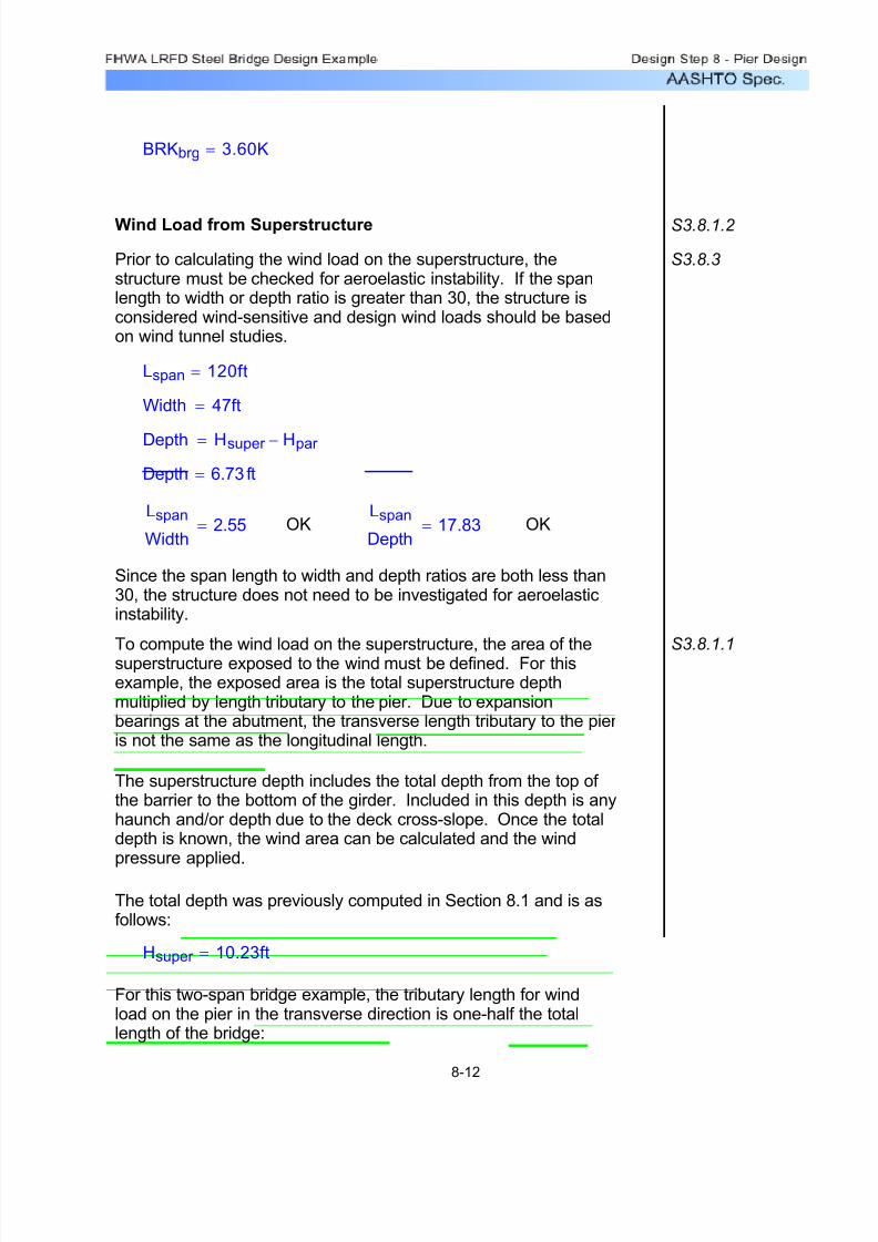
7/29/2019 LRFD steel design.pdf
http://slidepdf.com/reader/full/lrfd-steel-designpdf 474/646
For this two-span bridge example, the tributary length for windload on the pier in the transverse direction is one-half the totallength of the bridge:
Hsuper 10.23ft=
The total depth was previously computed in Section 8.1 and is asfollows:
The superstructure depth includes the total depth from the top of the barrier to the bottom of the girder. Included in this depth is anyhaunch and/or depth due to the deck cross-slope. Once the totaldepth is known, the wind area can be calculated and the windpressure applied.
S3.8.1.1To compute the wind load on the superstructure, the area of thesuperstructure exposed to the wind must be defined. For thisexample, the exposed area is the total superstructure depthmultiplied by length tributary to the pier. Due to expansionbearings at the abutment, the transverse length tributary to the pier is not the same as the longitudinal length.
Since the span length to width and depth ratios are both less than30, the structure does not need to be investigated for aeroelasticinstability.
OKLspan
Depth17.83=OK
Lspan
Width2.55=
Depth 6.73 ft=
Depth Hsuper Hpar −=
Width 47ft=
Lspan 120ft=
S3.8.3Prior to calculating the wind load on the superstructure, thestructure must be checked for aeroelastic instability. If the spanlength to width or depth ratio is greater than 30, the structure isconsidered wind-sensitive and design wind loads should be basedon wind tunnel studies.
S3.8.1.2 Wind Load from Superstructure
BRKbrg 3.60K=
8-12

7/29/2019 LRFD steel design.pdf
http://slidepdf.com/reader/full/lrfd-steel-designpdf 475/646
Windtotal 0.050ksf Hsuper ⋅=
S3.8.1.2.1 Also, the minimum transverse normal wind loading on girders mustbe greater than or equal to 0.30 KLF:
PD PB= PB
PD
PB
100mph
100mph
⎛
⎝
⎞
⎠
2
⋅= PB
or PD
PB
VDZ
VB
⎛
⎝
⎞
⎠
2
⋅= PB
S3.8.1.2.1 From this, the design wind pressure is equal to the base windpressure:
VDZ VB=
mphVB 100=
S3.8.1.1 Since the superstructure is approximately 30 feet above low groundlevel, the design wind velocity, VB, does not have to be adjusted.
Therefore:
AwsuperL 2455ft2=
AwsuperL Hsuper LwindL⋅=
The longitudinal wind area is:
AwsuperT
1228ft2=
AwsuperT Hsuper LwindT⋅=
The transverse wind area is:
LwindL 240ft=
In the longitudinal direction, the tributary length is the entire bridgelength due to the expansion bearings at the abutments:
LwindT 120ft=LwindT240
2ft=
8-13
= 120 x10.23
= klf
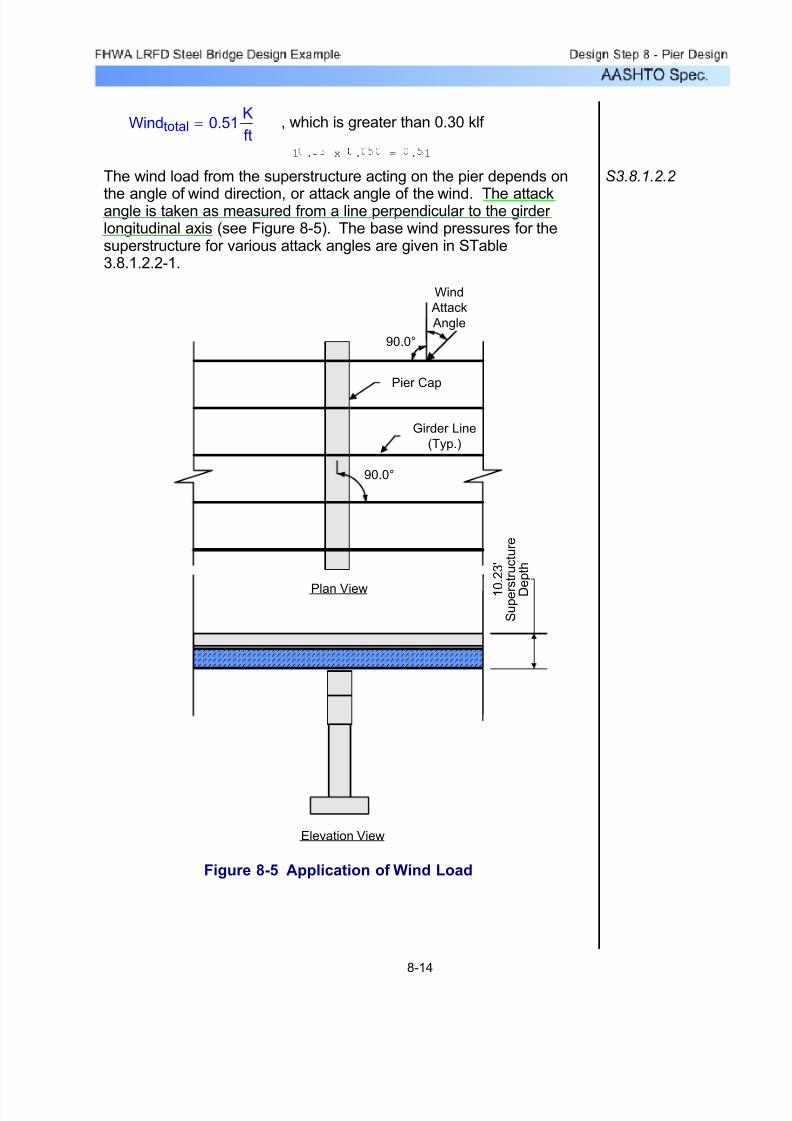
7/29/2019 LRFD steel design.pdf
http://slidepdf.com/reader/full/lrfd-steel-designpdf 476/646
Windtotal 0.51K
ft= , which is greater than 0.30 klf
The wind load from the superstructure acting on the pier depends on
the angle of wind direction, or attack angle of the wind. The attackangle is taken as measured from a line perpendicular to the girder longitudinal axis (see Figure 8-5). The base wind pressures for thesuperstructure for various attack angles are given in STable3.8.1.2.2-1.
S3.8.1.2.2
Plan View
Wind
Attack
Angle
Elevation View
Girder Line
(Typ.)
1 0
. 2 3 '
S u p e r s t r u c t u r e
D e p t h
90.0°
90.0°
Pier Cap
Figure 8-5 Application of Wind Load
8-14
1 . x . = . 1

7/29/2019 LRFD steel design.pdf
http://slidepdf.com/reader/full/lrfd-steel-designpdf 477/646
Table 8-1 Pier Design Wind Loads from Superstructure
for Various Wind Attack Angles
40.51 39.28
20.87 46.65
45
60
Kips Kips
61.38 0.00
54.01 14.73
50.33 29.46
Degrees
0
15
30
Bridge
Transverse Axis
Pier Design Wind Loads from
Superstructure
Bridge
Longitudinal Axis
Wind Attack
Angle
WSsuplng60 46.65K=
WSsuplng60 AwsuperL 0.019⋅ ksf =
WSsuptrns60 20.87K=
STable 3.8.1.2.2-1WSsuptrns60 AwsuperT 0.017⋅ ksf =
For a wind attack angle of 60 degrees, the superstructure wind loads
acting on the pier are:
WSsuplng0 0.00K=
WSsuplng0 AwsuperL 0.00⋅ ksf =
WSsuptrns0 61.38K=
STable 3.8.1.2.2-1WSsuptrns0 AwsuperT 0.050⋅ ksf =
For a wind attack angle of 0 degrees, the superstructure wind loadsacting on the pier are:
Two wind load calculations are illustrated below for two differentwind attack angles. The wind loads for all Specifications requiredattack angles are tabulated in Table 8-1.
8-15
A trans = 1
A long = 2455egrees trans =
perpendicular to
CL pie
t ese va ues rom ta e --->
egrees
sin 60 = .866
cos 60 = .5

7/29/2019 LRFD steel design.pdf
http://slidepdf.com/reader/full/lrfd-steel-designpdf 478/646
The total longitudinal wind load shown above for a given attack angle isassumed to be divided equally among the bearings. In addition, theload at each bearing is assumed to be applied at the top of the bearing(i.e., five inches above the pier cap). These assumptions are consistentwith those used in determining the bearing forces due to the longitudinalbraking force.
The transverse wind loads shown in Table 8-1 for a given attack angleare also assumed to be equally divided among the bearings andapplied at the top of each bearing. However, as shown in Figure 8-6,the transverse load also applies a moment to the pier cap. Thismoment, which acts about the centerline of the pier cap, inducesvertical loads at the bearings as illustrated in Figure 8-6. Thecomputations for these vertical forces with an attack angle of zero arepresented below.
4 Spaces @ 9’-9” = 39’-0”
46'-10½"
Figure 8-6 Transverse Wind Load Reactions at Pier Bearings
from Wind on Superstructure
Mtrns0 WSsuptrns0Hsuper
2
⎛ ⎝
⎞ ⎠
⋅=
Mtrns0 313.91K ft⋅=
Igirders 2 19.5ft( )2⋅ 2 9.75ft( )
2⋅+=
Igirders 950.63ft2=
RWS1_5trns0Mtrns0 19.5⋅ ft
Igirders=
RWS1_5trns0 6.44K=
8-16
= 61.38 x10.23/2

7/29/2019 LRFD steel design.pdf
http://slidepdf.com/reader/full/lrfd-steel-designpdf 479/646
This load causes a moment about the pier centerline. The value of this moment is:
WSvert 112.80K=
WSvert .02ksf Width( )⋅ LwindT( )⋅=
The total vertical wind load is then:
LwindT 120.00ft=
Width 47.00 ft=
From previous definitions:
The vertical (upward) wind load is calculated by multiplying a 0.020 ksf vertical wind pressure by the out-to-out bridge deck width. It is appliedat the windward quarter-point of the deck only for limit states that do notinclude wind on live load. Also, the wind attack angle must be zerodegrees for the vertical wind load to apply.
S3.8.2 Vertical Wind Load
The vertical reactions at the bearings due to transverse wind on thesuperstructure at attack angles other than zero are computed as aboveusing the appropriate transverse load from Table 8-1. Alternatively, thereactions for other attack angles can be obtained simply by multiplyingthe reactions obtained above by the ratio of the transverse load at theangle of interest to the transverse load at an attack angle of zero (i.e.,61.38K).
RWS3trns0 0.0K=
Finally, by inspection:
RWS2_4trns0 3.22K=
RWS2_4trns0
Mtrns0 9.75⋅ ft
Igirders=
The reactions at bearings 1 and 5 are equal but opposite in direction.Similarly for bearings 2 and 4:
8-17
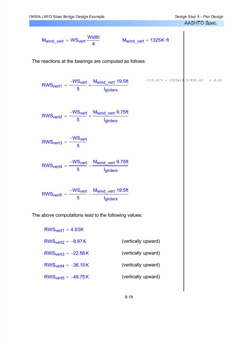
7/29/2019 LRFD steel design.pdf
http://slidepdf.com/reader/full/lrfd-steel-designpdf 480/646
(vertically upward)RWSvert5 49.75− K=
(vertically upward)RWSvert4 36.15− K=
(vertically upward)RWSvert3 22.56− K=
(vertically upward)RWSvert2 8.97− K=
RWSvert1 4.63K=
The above computations lead to the following values:
RWSvert5WSvert−
5
Mwind_vert 19.5⋅ ft
Igirders−=
RWSvert4WSvert−
5
Mwind_vert 9.75⋅ ft
Igirders−=
RWSvert3WSvert−
5=
RWSvert2WSvert−
5
Mwind_vert 9.75⋅ ft
Igirders
+=
RWSvert1WSvert−
5
Mwind_vert 19.5⋅ ft
Igirders+=
The reactions at the bearings are computed as follows:
Mwind_vert 1325K ft⋅=Mwind_vert WSvertWidth
4⋅=
8-18
-112.8/5 + 1325x19.5/950.63 = 4.61

7/29/2019 LRFD steel design.pdf
http://slidepdf.com/reader/full/lrfd-steel-designpdf 481/646
Wind Load on Vehicles S3.8.1.3
The representation of wind pressure acting on vehicular traffic is givenby the Specifications as a uniformly distributed load. Based on theskew angle, this load can act transversely, or both transversely and
longitudinally. Furthermore, this load is to be applied at a distance of six feet above the roadway surface. The magnitude of this load with awind attack angle of zero is 0.10 klf. For wind attack angles other than
zero, STable 3.8.1.3-1 gives values for the longitudinal and transversecomponents. For the transverse and longitudinal loadings, the totalforce in each respective direction is calculated by multiplying theappropriate component by the length of structure tributary to the pier.Similar to the superstructure wind loading, the longitudinal lengthtributary to the pier differs from the transverse length.
LwindT 120.00ft= LwindL 240.00ft=
An example calculation is illustrated below using a wind attack angle of 30 degrees:
WLtrans30 LwindT 0.082 klf ⋅( )⋅= STable 3.8.1.3-1
WLtrans30 9.84K=
WLlong30 LwindL 0.024klf ( )⋅= STable 3.8.1.3-1
WLlong30 5.76K=
Table 8-2 contains the total transverse and longitudinal loads due towind load on vehicular traffic at each Specifications required attackangle.
Design Vehicular Wind Loads
Wind Attack
Angle
Bridge
Transverse Axis
Bridge
Longitudinal Axis
Degrees Kips Kips
0 12.00 0.0015 10.56 2.88
30 9.84 5.76
45 7.92 7.68
60 4.08 9.12
Table 8-2 Design Vehicular Wind Loads for Various
Wind Attack Angles
8-19

7/29/2019 LRFD steel design.pdf
http://slidepdf.com/reader/full/lrfd-steel-designpdf 482/646
The vehicular live loads shown in Table 8-2 are applied to the bearingsin the same manner as the wind load from the superstructure. That is,the total transverse and longitudinal load is equally distributed to eachbearing and applied at the the top of the bearing (five inches above the
top of the pier cap). In addition, the transverse load acting six feetabove the roadway applies a moment to the pier cap. This momentinduces vertical reactions at the bearings. The values of these verticalreactions for a zero degree attack angle are given below. Thecomputations for these reactions are not shown but are carried out asshown in the subsection "Wind Load from Superstructure." The onlydifference is that the moment arm used for calculating the moment isequal to (Hsuper - Hpar + 6.0 feet).
RWL1_5trns0 3.13K=
RWL2_4trns0 1.57K=
RWL3trns0 0.0K=
Wind Load on Substructure S3.8.1.2.3
The Specifications state that the wind loads acting directly onsubstructure units shall be calculated from a base wind pressure of 0.040 ksf. It is interpreted herein that this pressure should be applied tothe projected area of the pier that is normal to the wind direction. Thisis illustrated in Figure 8-7. The resulting force is then the product of 0.040 ksf and the projected area. For nonzero wind attack angles, thisforce is resolved into components applied to the front and endelevations of the pier, respectively. These loads act simultaneously withthe superstructure wind loads.
8-20
see page -1
w = 12k, M = 12 x (10.23-3.5-6) =152.76
R = 152.76 x 19.5/950.03 = 3.13

7/29/2019 LRFD steel design.pdf
http://slidepdf.com/reader/full/lrfd-steel-designpdf 483/646
Pier Cap
Plan View
Wind
Attack
Angle
θ θ
θ
Projected
Face
Projected
Face
Figure 8-7 Projected Area for Wind Pressure on Pier
What follows is an example of the calculation of the wind loads actingdirectly on the pier for a wind attack angle of 30 degrees. For simplicity,the tapers of the pier cap overhangs will be considered solid (this isconservative and helpful for wind angles other than zero degrees). Thecolumn height exposed to wind is the distance from the ground line(which is two feet above the footing) to the bottom of the pier cap.
Component areas of the pier cap:
Acap1 11.0ft( ) 5.0ft( )⋅= Acap1 55.00ft2=
Acap2 11.0ft( ) 46.5ft( )⋅= Acap2 511.50ft2=
8-21
transverse
longitudinal
Included the hatched area in the example

7/29/2019 LRFD steel design.pdf
http://slidepdf.com/reader/full/lrfd-steel-designpdf 484/646
The point of application of these loads will be the centroid of the loadedarea of each face, respectively. This point will be approximated here as17 feet above the top of the footing for both the transverse andlongitudinal directions.
WSsub30L 9.10K=
WSsub30T 15.75K=
WSsub30L WSsub30 sin 30 deg⋅( )⋅=
WSsub30T WSsub30 cos 30 deg⋅( )⋅=
The transverse and longitudinal force components are:
WSsub30 18.19K=
WSsub30 0.040ksf APcap APcol+( )⋅=
The total wind force is then:
APcol 151.41ft2=
APcol Acol1 cos 30 deg⋅( )⋅ Acol2 sin 30 deg⋅( )⋅+=
Projected area of pier column:
Acol2 201.50ft2= Acol2 15ft 2ft−( ) 15.5ft( )⋅=
Acol1 58.50ft2= Acol1 15ft 2ft−( ) 4.5ft( )⋅=
Component areas of the pier column:
APcap 303.38ft
2
=
APcap Acap1 cos 30 deg⋅( )⋅ Acap2 sin 30 deg⋅( )⋅+=
Projected area of pier cap:
8-22
See "Additional No

7/29/2019 LRFD steel design.pdf
http://slidepdf.com/reader/full/lrfd-steel-designpdf 485/646
The wind attack angles for the pier must match the wind attack anglesused for the superstructure. Table 8-3 shows the pier wind loads for thevarious attack angles.
APcap APcol
Total
Wind
Load
ft2
ft2
Kips
55.00 58.50 4.54185.51 108.66 11.77
303.38 151.41 18.19
400.58 183.85 23.38
470.47 203.75 26.97
Wind Loads
Applied Directly
to Pier
Wind
Attack
Angle
Trans.
Force
Long.
Force
Degrees Kips Kips
0 4.54 0.0015 11.37 3.05
30 15.75 9.10
45 16.53 16.53
60 13.49 23.36
Table 8-3 Design Wind Loads Applied Directly to Pier for Various
Wind Attack Angles
Earthquake Load S3.10
It is assumed in this design example that the structure is located inSeismic Zone I with an acceleration coefficient of 0.02. For Seismic Zone I, a seismic analysis is not required. However, theSpecifications require a minimum design force for the check of thesuperstructure to substructure connection. Also, at locations of expansion bearings, a minimum bridge seat must be provided.
S4.7.4.1
S3.10.9
S4.7.4.4
Since the bearings at the pier are fixed both longitudinally andtransversely, minimum bridge seat requirements for seismic loads arenot applicable. Also, since the bearing design is carried out in DesignStep 6, the calculations for the check of the connection will not beshown here. Therefore, the earthquake provisions as identified in theabove paragraph will have no impact on the overall pier design andwill not be discussed further.
8-23

7/29/2019 LRFD steel design.pdf
http://slidepdf.com/reader/full/lrfd-steel-designpdf 486/646
Temperature Loading (Superimposed Deformations) S3.12
In general, uniform thermal expansion and contraction of thesuperstructure can impose longitudinal forces on the substructureunits. These forces can arise from restraint of free movement at the
bearings. Additionally, the physical locations and number of substructure units can cause or influence these forces.
S3.12.2
STable 3.12.2.1-1
In this particular structure, with a single pier centered between twoabutments that have identical bearing types, theoretically no force willdevelop at the pier from thermal movement of the superstructure.However, seldom are ideal conditions achieved in a physical structure.Therefore, it is considered good practice to include an approximatethermal loading even when theory indicates the absence of any suchforce.
For the purpose of this design example, a total force of 20 kips will beassumed. This force acts in the longitudinal direction of the bridge(either back or ahead station) and is equally divided among thebearings. Also, the forces at each bearing from this load will beapplied at the top of the bearing (i.e., five inches above the pier cap).
TU1 4.0K=
TU2 4.0K=
TU3 4.0K=
TU4 4.0K=
TU5 4.0K=
Design Step 8.7 - Analyze and Combine Force Effects
The first step within this design step will be to summarize the loadsacting on the pier at the bearing locations. This is done in Tables 8-4through 8-15 shown below. Tables 8-4 through 8-8 summarize thevertical loads, Tables 8-9 through 8-12 summarize the horizontallongitudinal loads, and Tables 8-13 through 8-15 summarize thehorizontal transverse loads. These loads along with the pier self-weight loads, which are shown after the tables, need to be factoredand combined to obtain total design forces to be resisted in the pier cap, column and footing.
8-24
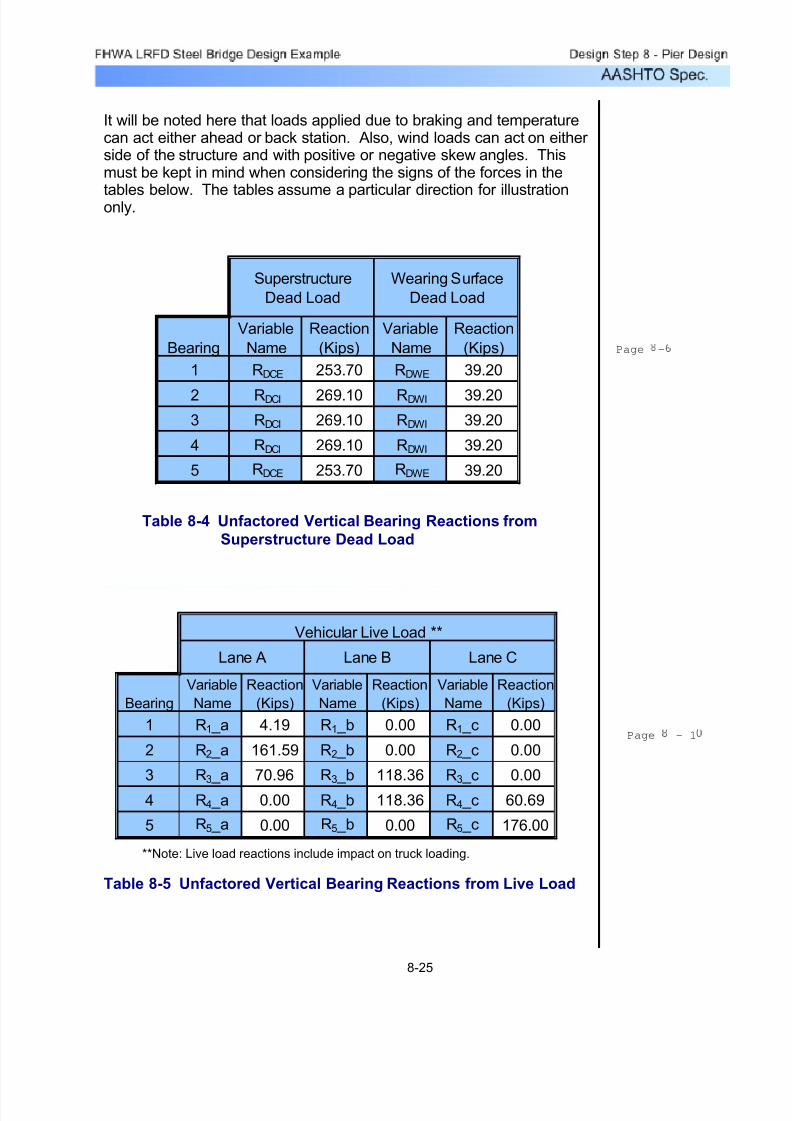
7/29/2019 LRFD steel design.pdf
http://slidepdf.com/reader/full/lrfd-steel-designpdf 487/646
It will be noted here that loads applied due to braking and temperaturecan act either ahead or back station. Also, wind loads can act on either side of the structure and with positive or negative skew angles. Thismust be kept in mind when considering the signs of the forces in the
tables below. The tables assume a particular direction for illustrationonly.
Bearing
Variable
Name
Reaction
(Kips)
Variable
Name
Reaction
(Kips)
1 RDCE 253.70 RDWE 39.20
2 RDCI 269.10 RDWI 39.20
3 RDCI 269.10 RDWI 39.20
4 RDCI 269.10 RDWI 39.20
5 RDCE 253.70 RDWE 39.20
Superstructure
Dead Load
Wearing Surface
Dead Load
Table 8-4 Unfactored Vertical Bearing Reactions from
Superstructure Dead Load
Bearing
Variable
Name
Reaction
(Kips)
Variable
Name
Reaction
(Kips)
Variable
Name
Reaction
(Kips)
1 R1 _a 4.19 R1 _b 0.00 R1 _c 0.00
2 R2 _a 161.59 R2 _b 0.00 R2 _c 0.00
3 R3 _a 70.96 R3 _b 118.36 R3 _c 0.00
4 R4 _a 0.00 R4 _b 118.36 R4 _c 60.69
5 R5 _a 0.00 R5 _b 0.00 R5 _c 176.00
Lane A Lane B Lane C
Vehicular Live Load **
**Note: Live load reactions include impact on truck loading.
Table 8-5 Unfactored Vertical Bearing Reactions from Live Load
8-25
Page -
Page - 1
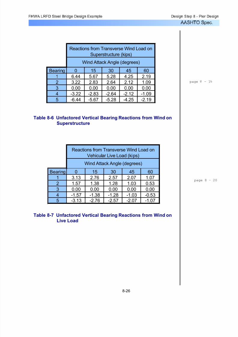
7/29/2019 LRFD steel design.pdf
http://slidepdf.com/reader/full/lrfd-steel-designpdf 488/646
Bearing 0 15 30 45 60
1 6.44 5.67 5.28 4.25 2.19
2 3.22 2.83 2.64 2.12 1.09
3 0.00 0.00 0.00 0.00 0.00
4 -3.22 -2.83 -2.64 -2.12 -1.09
5 -6.44 -5.67 -5.28 -4.25 -2.19
Wind Attack Angle (degrees)
Reactions from Transverse Wind Load on
Superstructure (kips)
Table 8-6 Unfactored Vertical Bearing Reactions from Wind onSuperstructure
Bearing 0 15 30 45 60
1 3.13 2.76 2.57 2.07 1.072 1.57 1.38 1.28 1.03 0.53
3 0.00 0.00 0.00 0.00 0.00
4 -1.57 -1.38 -1.28 -1.03 -0.53
5 -3.13 -2.76 -2.57 -2.07 -1.07
Wind Attack Angle (degrees)
Reactions from Transverse Wind Load on
Vehicular Live Load (kips)
Table 8-7 Unfactored Vertical Bearing Reactions from Wind on
Live Load
8-26
page - 1
page 8 - 20

7/29/2019 LRFD steel design.pdf
http://slidepdf.com/reader/full/lrfd-steel-designpdf 489/646
Bearing
Variable
Name
Reaction
(Kips)
1 RWSvert1 4.63
2 RWSvert2 -8.97
3 RWSvert3 -22.56
4 RWSvert4 -36.15
5 RWSvert5 -49.75
Vertical Wind Load
on Superstructure
Table 8-8 Unfactored Vertical Bearing Reactions from Vertical
Wind on Superstructure
BearingVariable
NameReaction
(Kips)Variable
NameReaction
(Kips)
1 BRKbrg 3.60 TU1 4.00
2 BRKbrg 3.60 TU2 4.00
3 BRKbrg 3.60 TU3 4.00
4 BRKbrg 3.60 TU4 4.00
5 BRKbrg 3.60 TU5 4.00
Braking Load **Temperature
Loading
**Note: Values shown are for a single lane loaded
Table 8-9 Unfactored Horizontal Longitudinal Bearing
Reactions from Braking and Temperature
8-27
Page -
page 8 - 11 (B)
page 8 - 24 (T)
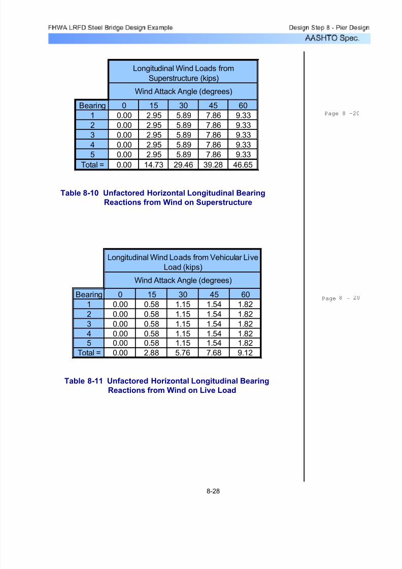
7/29/2019 LRFD steel design.pdf
http://slidepdf.com/reader/full/lrfd-steel-designpdf 490/646
Bearing 0 15 30 45 60
1 0.00 2.95 5.89 7.86 9.33
2 0.00 2.95 5.89 7.86 9.33
3 0.00 2.95 5.89 7.86 9.33
4 0.00 2.95 5.89 7.86 9.33
5 0.00 2.95 5.89 7.86 9.33
Total = 0.00 14.73 29.46 39.28 46.65
Wind Attack Angle (degrees)
Longitudinal Wind Loads from
Superstructure (kips)
Table 8-10 Unfactored Horizontal Longitudinal Bearing
Reactions from Wind on Superstructure
Bearing 0 15 30 45 60
1 0.00 0.58 1.15 1.54 1.82
2 0.00 0.58 1.15 1.54 1.82
3 0.00 0.58 1.15 1.54 1.82
4 0.00 0.58 1.15 1.54 1.82
5 0.00 0.58 1.15 1.54 1.82
Total = 0.00 2.88 5.76 7.68 9.12
Wind Attack Angle (degrees)
Longitudinal Wind Loads from Vehicular Live
Load (kips)
Table 8-11 Unfactored Horizontal Longitudinal Bearing
Reactions from Wind on Live Load
8-28
Page 8 -20
Page -

7/29/2019 LRFD steel design.pdf
http://slidepdf.com/reader/full/lrfd-steel-designpdf 491/646
0 15 30 45 60
0.00 3.05 9.10 16.53 23.36
Wind Attack Angle (degrees)
Longitudinal Substructure Wind Loads
Applied Directly to Pier (kips)
Table 8-12 Unfactored Horizontal Longitudinal Loads
from Wind Directly on Pier
Bearing 0 15 30 45 60
1 12.28 10.80 10.07 8.10 4.17
2 12.28 10.80 10.07 8.10 4.17
3 12.28 10.80 10.07 8.10 4.17
4 12.28 10.80 10.07 8.10 4.17
5 12.28 10.80 10.07 8.10 4.17
Total = 61.38 54.01 50.33 40.51 20.87
Wind Attack Angle
Transverse Wind Loads from
Superstructure
Table 8-13 Unfactored Horizontal Transverse Bearing
Reactions from Wind on Superstructure
8-29
Page -
Page -1 ; va ues are
divided by number of girders
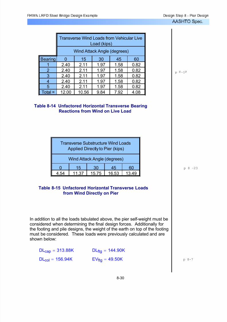
7/29/2019 LRFD steel design.pdf
http://slidepdf.com/reader/full/lrfd-steel-designpdf 492/646
Bearing 0 15 30 45 60
1 2.40 2.11 1.97 1.58 0.82
2 2.40 2.11 1.97 1.58 0.82
3 2.40 2.11 1.97 1.58 0.82
4 2.40 2.11 1.97 1.58 0.825 2.40 2.11 1.97 1.58 0.82
Total = 12.00 10.56 9.84 7.92 4.08
Wind Attack Angle (degrees)
Transverse Wind Loads from Vehicular Live
Load (kips)
Table 8-14 Unfactored Horizontal Transverse Bearing
Reactions from Wind on Live Load
0 15 30 45 604.54 11.37 15.75 16.53 13.49
Wind Attack Angle (degrees)
Transverse Substructure Wind Loads
Applied Directly to Pier (kips)
Table 8-15 Unfactored Horizontal Transverse Loads
from Wind Directly on Pier
In addition to all the loads tabulated above, the pier self-weight must be
considered when determining the final design forces. Additionally for the footing and pile designs, the weight of the earth on top of the footingmust be considered. These loads were previously calculated and areshown below:
DLcap 313.88K= DLftg 144.90K=
DLcol 156.94K= EVftg 49.50K=
8-30
p -1
p 8 -23
p 8-7

7/29/2019 LRFD steel design.pdf
http://slidepdf.com/reader/full/lrfd-steel-designpdf 493/646
S3.4.1 It is important to note here that the maximum load factors shown inTable 8-16 for uniform temperature loading (TU) apply only for deformations, and the minimum load factors apply for all other effects.Since the force effects from the uniform temperature loading are
considered in this pier design, the minimum load factors will be used.
Table 8-16 contains the applicable limit states and correspondingload factors that will be used for this pier design. Limit states notshown either do not control the design or are not applicable. Theload factors shown in Table 8-16 are the standard load factorsassigned by the Specifications and are exclusive of multiplepresence and eta factors.
m3 0.85=Multiple presence factor, m (3 lanes)
m2 1.00=Multiple presence factor, m (2 lanes)
m1 1.20=Multiple presence factor, m (1 lane)
STable 3.6.1.1.2-1The other set of factors mentioned in the first paragraph above appliesonly to the live load force effects and are dependent upon the number of loaded lanes. These factors are termed multiple presence factorsby the Specifications. These factors for this bridge are shown asfollows:
S1.3.2.1The first set of additional factors applies to all force effects and arerepresented by the Greek letter η (eta) in the Specifications. These
factors are related to the ductility, redundancy, and operationalimportance of the structure. A single, combined eta is required for every structure. These factors and their application are discussed indetail in Design Step 1.1. In this design example, all eta factors aretaken equal to one.
STable 3.4.1-2
STable 3.4.1-1In the AASHTO LRFD design philosophy, the applied loads arefactored by statistically calibrated load factors. In addition to thesefactors, one must be aware of two additional sets of factors whichmay further modify the applied loads.
8-31
age -

7/29/2019 LRFD steel design.pdf
http://slidepdf.com/reader/full/lrfd-steel-designpdf 494/646
Load γmax γmin γmax γmin γmax γmin γmax γmin
DC 1.25 0.90 1.25 0.90 1.25 0.90 1.00 1.00
DW 1.50 0.65 1.50 0.65 1.50 0.65 1.00 1.00
LL 1.75 1.75 --- --- 1.35 1.35 1.00 1.00
BR 1.75 1.75 --- --- 1.35 1.35 1.00 1.00
TU 1.20 0.50 1.20 0.50 1.20 0.50 1.20 1.00
WS --- --- 1.40 1.40 0.40 0.40 0.30 0.30
WL --- --- --- --- 1.00 1.00 1.00 1.00
EV 1.35 1.00 1.35 1.00 1.35 1.00 1.00 1.00
Strength V Service I
Load Factors
Strength I Strength III
STable 3.4.1-1
STable 3.4.1-2
Table 8-16 Load Factors and Applicable Pier Limit States
The loads discussed and tabulated previously can now be factored bythe appropriate load factors and combined to determine the governinglimit states in the pier cap, column, footing and piles. For this designexample, the governing limit states for the pier components weredetermined from a commercially available pier design computer program. Design calculations will be carried out for the governing limitstates only.
Pier Cap Force Effects
The controlling limit states for the design of the pier cap are Strength I(for moment, shear and torsion) and Service I ( for crack control). Thecritical design location is where the cap meets the column, or 15.5 feetfrom the end of the cap. This is the location of maximum moment,shear, and torsion. The reactions at the two outermost bearings(numbered 4 and 5 in Figure 8-4), along with the self-weight of the capoverhang, cause the force effects at the critical section. In the followingcalculations, note that the number of lanes loaded to achieve themaximum moment is different than that used to obtain the maximum
shear and torsion.
For Strength I, the factored vertical and horizontal forces at the bearingsand corresponding force effects at the critical section are shown below.
Also shown are the moment arms to the critical section.
Flexure from vertical loads (reference Tables 8-4 and 8-5):
FV4cap_flexstr1 1.25 RDCI⋅ 1.50 RDWI⋅+ 1.75 R4_c⋅ m1⋅+=
8-32
This is the pier cap
overhang
page 8-25
m1 - see page - 1
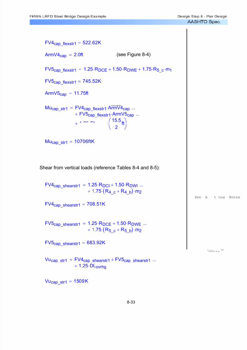
7/29/2019 LRFD steel design.pdf
http://slidepdf.com/reader/full/lrfd-steel-designpdf 495/646
FV4cap_flexstr1 522.62K=
ArmV4cap 2.0ft= (see Figure 8-4)
FV5cap_flexstr1 1.25 RDCE⋅ 1.50 RDWE⋅+ 1.75 R5_c⋅ m1⋅+=
FV5cap_flexstr1 745.52K=
ArmV5cap 11.75ft=
Mucap_str1 FV4cap_flexstr1 ArmV4cap⋅FV5cap_flexstr1 ArmV5cap⋅+
...
1.25 DLovrhg⋅ 15.52
ft⎛ ⎝ ⎞ ⎠⋅+
...=
Mucap_str1 10706ftK=
Shear from vertical loads (reference Tables 8-4 and 8-5):
FV4cap_shearstr1 1.25 RDCI⋅ 1.50 RDWI⋅+1.75 R4_c R4_b+( )⋅ m2⋅+
...=
FV4cap_shearstr1 708.51K=
FV5cap_shearstr1 1.25 RDCE⋅ 1.50 RDWE⋅+1.75 R5_c R5_b+( )⋅ m2⋅+
...=
FV5cap_shearstr1
683.92K=
Vucap_str1 FV4cap_shearstr1 FV5cap_shearstr1+1.25 DLovrhg⋅+
...=
Vucap_str1 1509K=
8-33
See A t ona N

7/29/2019 LRFD steel design.pdf
http://slidepdf.com/reader/full/lrfd-steel-designpdf 496/646
RWL4trans0 1.57K=RWS4trans0 3.22K=
RWL5trans0 3.13K=RWS5trans0 6.44K=
S3.8.2
For Service I, the factored vertical forces at the bearings andcorresponding force effects at the critical section are shown next.First, variables for transverse wind load on the structure and on the live
load with an attack angle of zero degrees will be defined. Forceeffects from vertical wind load on the structure are not applicable sincethe Service I limit state includes wind on live load.
The applied torsion would be larger than the value just calculated if thevertical loads at the bearings are not coincident with the centerline of the pier cap. Some state agencies mandate a minimum eccentricity toaccount for this possibility. However, AASHTO does not. Therefore,no eccentricity of vertical loads is considered in this design example.
Tucap_str1 172.77ftK=
Tucap_str1 FH4cap_torstr1 FH5cap_torstr1+( ) ArmHcap⋅=
ArmHcap 5.92ft=
ArmHcap11
2
ftHbrng
12 inft
+=
FH5cap_torstr1 14.60K=
FH5cap_torstr1 2 1.75 BRKbrg⋅ m2⋅( )⋅ 0.50 TU5⋅+=
FH4cap_torstr1 14.60K=
FH4cap_torstr1 2 1.75 BRKbrg⋅ m2⋅( )⋅ 0.50 TU4⋅+=
Torsion from horizontal loads (reference Table 8-9):
8-34
See "Additional No

7/29/2019 LRFD steel design.pdf
http://slidepdf.com/reader/full/lrfd-steel-designpdf 497/646
Flexure from vertical loads (reference Tables 8-4 and 8-5):
FV4cap_flexser1 1.00 RDCI⋅ 1.00 RDWI⋅+ 1.00 R4_c⋅ m1⋅+0.30 RWS4trans0⋅ 1.00 RWL4trans0⋅++
...=
FV4cap_flexser1 383.66K=
Arm4V 2.0ft= (see Figure 8-4)
FV5cap_flexser1 1.00 RDCE⋅ 1.00 RDWE⋅+ 1.00 R5_c⋅ m1⋅+0.30 RWS5trans0⋅ 1.00 RWL5trans0⋅++
...=
FV5cap_flexser1 509.16K=
Arm5V 11.75ft=
Mucap_ser1 FV4cap_flexser1 Arm4V⋅ FV5cap_flexser1 Arm5V⋅+
1.00 DLovrhg⋅15.5
2
ft⎛
⎝
⎞
⎠
⋅+
...=
Mucap_ser1 7471ftK=
Pier Column Force Effects
The controlling limit states for the design of the pier column areStrength I (for biaxial bending with axial load), Strength III (for
transverse shear) and Strength V (for longitudinal shear). The criticaldesign location is where the column meets the footing, or at thecolumn base. The governing force effects for Strength I are achievedby excluding the future wearing surface, applying minimum loadfactors on the structure dead load, and loading only Lane B and LaneC with live load. Transverse and longitudinal shears are maximizedwith wind attack angles of zero and 60 degrees, respectively.
8-35
See "Additional Not
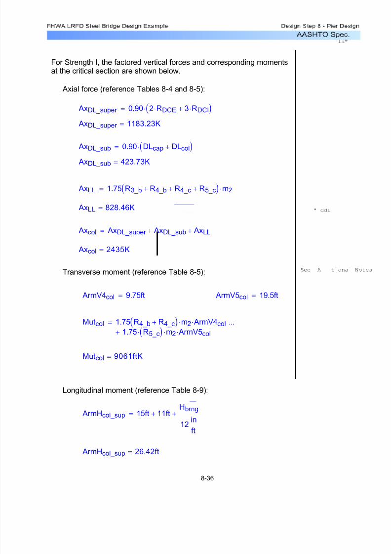
7/29/2019 LRFD steel design.pdf
http://slidepdf.com/reader/full/lrfd-steel-designpdf 498/646
ArmHcol_sup 26.42ft=
ArmHcol_sup 15ft 11ft+Hbrng
12in
ft
+=
Longitudinal moment (reference Table 8-9):
Mutcol 9061ftK=
Mutcol 1.75 R4_b R4_c+( ) m2⋅ ArmV4col⋅1.75 R5_c( )⋅ m2⋅ ArmV5col⋅+
...=
ArmV5col 19.5ft= ArmV4col 9.75ft=
Transverse moment (reference Table 8-5):
Axcol 2435K=
Axcol AxDL_super AxDL_sub+ AxLL+=
AxLL 828.46K=
AxLL 1.75 R3_b R4_b+ R4_c+ R5_c+( ) m2⋅=
AxDL_sub 423.73K=
AxDL_sub 0.90 DLcap DLcol+( )⋅=
AxDL_super 1183.23K=
AxDL_super 0.90 2 RDCE⋅ 3 RDCI⋅+( )⋅=
Axial force (reference Tables 8-4 and 8-5):
For Strength I, the factored vertical forces and corresponding momentsat the critical section are shown below.
8-36
See A t ona Not

7/29/2019 LRFD steel design.pdf
http://slidepdf.com/reader/full/lrfd-steel-designpdf 499/646
Mulcol 5 1.75 BRKbrg⋅ ArmHcol_sup⋅( )⋅ 2⋅ m2⋅0.50 TU1 TU2+
TU3 TU4+ TU5++...⎛
⎝ ⎞ ⎠
ArmHcol_sup⋅+...=
Mulcol 1928ftK=
For Strength III, the factored transverse shear in the column is:
WSsuptrns0 61.38K= WSsub0T 4.54K=
Vutcol 1.40 WSsuptrns0 WSsub0T+( )=
Vutcol 92.28K=
For Strength V, the factored longitudinal shear in the column is(reference Table 8-9):
WSsuplng60 46.65K= WSsub60L 23.36K=
WLlong60 9.12K=
Vulcol 0.40 WSsuplng60 WSsub60L+( ) 1.00 WLlong60⋅+0.50 TU1 TU2+ TU3+ TU4+ TU5+( )⋅+
...
1.35 5 BRKbrg⋅( )⋅ 3⋅ m3⋅+...
=
Vulcol 109.09K=
Pier Pile Force Effects
The foundation system for the pier is a reinforced concrete footing onsteel H-piles. The force effects in the piles cannot be determinedwithout a pile layout. The pile layout depends upon the pile capacityand affects the footing design. The pile layout used for this pier foundation is shown in Design Step 8.10 (Figure 8-11).
8-37
See A t ona No

7/29/2019 LRFD steel design.pdf
http://slidepdf.com/reader/full/lrfd-steel-designpdf 500/646
Based on the pile layout shown in Figure 8-11, the controlling limitstates for the pile design are Strength I (for maximum pile load),Strength III (for minimum pile load), and Strength V (for maximumhorizontal loading of the pile group).
The force effects in the piles for the above-mentioned limit states arenot given. The reason for this is discussed in Design Step 8.10.
Pier Footing Force Effects
The controlling limit states for the design of the pier footing areStrength I (for flexure, punching shear at the column, and punchingshear at the maximum loaded pile), Strength IV (for one-way shear),and Service I ( for crack control). There is not a single critical designlocation in the footing where all of the force effects just mentioned are
checked. Rather, the force effects act at different locations in thefooting and must be checked at their respective locations. For example, the punching shear checks are carried out using criticalperimeters around the column and maximum loaded pile, while theflexure and one-way shear checks are carried out on a vertical face of the footing either parallel or perpendicular to the bridge longitudinalaxis.
The Strength I limit state controls for the punching shear check at thecolumn. The factored axial load and corresponding factored biaxialmoments at the base of the column are obtained in a manner similar tothat for the Strength I force effects in the pier column. However, in this
case the future wearing surface is now included, maximum factors areapplied to all the dead load components, and all three lanes areloaded with live load. This results in the following bottom of columnforces:
Axcol_punch 3583K=
Mutcol_punch 5287ft K⋅=
Mulcol_punch 2756ft K⋅=
Factored force effects for the remaining limit states discussed aboveare not shown. The reason for this is discussed in Design Step 8.11.
8-38

7/29/2019 LRFD steel design.pdf
http://slidepdf.com/reader/full/lrfd-steel-designpdf 501/646
Mucap_ser1 7471ftK=
Service I
Tucap_str1 172.77ftK=
Vucap_str1 1509K=
Mucap_str1 10706ftK=
Strength I
As stated in Design Step 8.7, the critical section in the pier cap is wherethe cap meets the column, or 15.5' from the end of the cap. Thegoverning force effects and their corresponding limit states weredetermined to be:
The design of the pier cap will now proceed.
For the purpose of this design example, all structural components,regardless of dimensions, will be designed in accordance with theconventional strength of materials assumptions described above. Thisapproach is currently standard engineering practice.
C5.6.3.1
Traditionally, piers have been designed using conventional methods of
strength of materials regardless of member dimensions. In thisapproach, it is assumed that longitudinal strains vary linearly over thedepth of the member and the shear distribution remains uniform.Furthermore, separate designs are carried out for Vu and Mu at differentlocations along the member.
S5.6.3.1
S5.2 When a structural member meets the definition of a deep component,the Specifications recommends, although does not mandate, that astrut-and-tie model be used to determine force effects and required
reinforcing. Specifications Commentary C5.6.3.1 indicates that astrut-and-tie model properly accounts for nonlinear strain distribution,nonuniform shear distribution, and the mechanical interaction of Vu, Tu and Mu. Use of strut-and-tie models for the design of reinforcedconcrete members is new to the LRFD Specification.
Prior to carrying out the actual design of the pier cap, a brief discussionis in order regarding the design philosophy that will be used for the
design of the structural components of this pier.
Design Step 8.8 - Design Pier Cap
8-39
-
8-33
-
-

7/29/2019 LRFD steel design.pdf
http://slidepdf.com/reader/full/lrfd-steel-designpdf 502/646
A preliminary estimate of the required section size and reinforcement isshown in Figure 8-8.
1 1 ' - 0 "
1 2 5
. 9 7 i n
.
3 "
2 rows of 10 -
#11 bars
5'-0"
#5 hoops @
9" O.C. (typ)
2 1/2"
clear
(typ)
c l e a r
( t y p ) #8 bars @ 8" O.C.
(typ - side faces)
#8 bars @ 12"
O.C. - bottom
face
d e
=
Figure 8-8 Preliminary Pier Cap Design
Design for Flexure (Strength I)
Assume #11 bars:
bar_diam11 1.41in=
bar_area11 1.56in2=
f y 60ksi=
The minimum reinforcement requirements will be calculated for thecap. The tensile reinforcement provided must be enough to develop afactored flexural resistance at least equal to the lesser of 1.2 times thecracking strength or 1.33 times the factored moment from theapplicable strength load combinations.
S5.7.3.3.2
8-40

7/29/2019 LRFD steel design.pdf
http://slidepdf.com/reader/full/lrfd-steel-designpdf 503/646
f c 4.0ksi=
b 60in=
S5.5.4.2.1φf 0.90=
Solve for the required amount of reinforcing steel, as follows:
de 125.97in=
de 132in Cover cp .625in+ 1.41in+3
2in+⎛
⎝ ⎞ ⎠
−=
Cover cp 2.50in=
The effective depth (de) of the section shown in Figure 8-8 is computedas follows:
By inspection, the applied moment from the Strength I limit stateexceeds 120 percent of the cracking moment. Therefore, providingsteel sufficient to resist the applied moment automatically satisfies the
minimum reinforcement check.
1.2 Mcr ⋅ 8364ftK=
Mcr 6970ftK=
Mcr f r Ig⋅
yt
1
12 inft
⋅=
yt 66in=
Ig 11499840in4=
Ig1
1260in( ) 132in( )
3=
f r 0.48ksi=
S5.4.2.6 f r 0.24 f c⋅= f c
The cracking strength is calculated as follows:
8-41
=133/2

7/29/2019 LRFD steel design.pdf
http://slidepdf.com/reader/full/lrfd-steel-designpdf 504/646
OK0.09 0.42≤
S5.7.3.3.1c
de0.42≤where
c
de0.09=
S5.7.2.2 c 10.80 in=ca
β1
=
S5.7.2.2 β1 0.85=
a 9.18in=aT
0.85 f c⋅ b⋅=
T 1872.00 K=T As_cap f y⋅=
S5.7.3.3.1The reinforcement area provided must now be checked to ensure thatthe section is not overreinforced:
OK As_cap As≥
As_cap 31.20in2=
As_cap 20 bar_area11( )⋅=
The area of steel provided is:
As 19.32in2= As ρ b⋅ de⋅=
The above two equations are derived formulas that can be found in
most reinforced concrete textbooks.
ρ 0.00256=
ρ 0.85f c
f y
⎛
⎝
⎞
⎠1.0 1.0
2 Rn⋅( )
0.85 f c⋅( )−−⎡
⎣⎤⎦
⋅=
Rn 0.15ksi=Rn
Mucap_str1 12⋅in
ft
φf b⋅ de2⋅( )=
Mucap_str1 10706ftK=
8-42
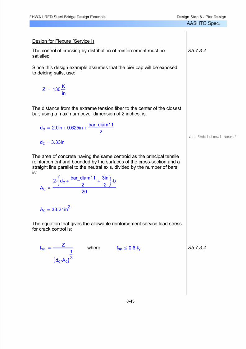
7/29/2019 LRFD steel design.pdf
http://slidepdf.com/reader/full/lrfd-steel-designpdf 505/646
S5.7.3.4f sa 0.6 f y⋅≤wheref saZ
dc Ac⋅( )
1
3
=
The equation that gives the allowable reinforcement service load stressfor crack control is:
Ac 33.21in2=
Ac2 dc
bar_diam11
2+
3in
2+
⎛
⎝
⎞
⎠⋅ b⋅20
=
The area of concrete having the same centroid as the principal tensilereinforcement and bounded by the surfaces of the cross-section and astraight line parallel to the neutral axis, divided by the number of bars,is:
dc 3.33in=
dc 2.0in 0.625in+bar_diam11
2+=
The distance from the extreme tension fiber to the center of the closestbar, using a maximum cover dimension of 2 inches, is:
Z 130K
in=
Since this design example assumes that the pier cap will be exposedto deicing salts, use:
S5.7.3.4The control of cracking by distribution of reinforcement must besatisfied.
Design for Flexure (Service I)
8-43
See "Additional Not

7/29/2019 LRFD steel design.pdf
http://slidepdf.com/reader/full/lrfd-steel-designpdf 506/646
k de⋅ 28.48in=
k 0.226=
k ρ n⋅( )2
2 ρ⋅ n⋅( )+ ρ n⋅−=
ρ 0.00413=ρ As_cap
b de⋅=
As_cap 31.20in2=de 125.97in=
n 8=
To solve for the actual stress in the reinforcement, the distance from theneutral axis to the centroid of the reinforcement (see Figure 8-9) and thetransformed moment of inertia must be computed:
Mucap_ser1 7471ftK=
The factored service moment in the cap is:
n 8=Usen 7.97=nEs
Ec=
SEquation
C5.4.2.4-1Ec 3640ksi=
S5.4.3.2 Es 29000ksi=
f sa 27.08ksi=Use
0.6f y 36.00ksi=f sa 27.08ksi=
8-44
page -

7/29/2019 LRFD steel design.pdf
http://slidepdf.com/reader/full/lrfd-steel-designpdf 507/646
1 3 2
. 0 0 i n
.
2 8 . 4 8 i n
.
Centroidal Axis
60.00in.
9 7
. 4 9 i n
.
Figure 8-9 Pier Cap Under Service Loads
Once kde is known, the transformed moment of inertia can becomputed:
de 125.97in=
As_cap 31.20in2=
It1
360in( )⋅ k de⋅( )3⋅ n As_cap⋅ de k de⋅−( )2⋅+=
It 2834038in4=
Now, the actual stress in the reinforcement is computed:
Mucap_ser1 7471ftK=
y de k de⋅−= y 97.49 in=
f s
Mucap_ser1 12⋅in
fty⋅⎛
⎝ ⎞ ⎠
Itn⋅=
8-45

7/29/2019 LRFD steel design.pdf
http://slidepdf.com/reader/full/lrfd-steel-designpdf 508/646
31.2
4
⎛ ⎝
⎞ ⎠
in2
ft⋅ 7.80
in2
ft=
(each side face) Ask 1.15in
2
ft=
Ask 0.012 125.97 30−( )⋅
in2
ft=
SEquation
5.7.3.4-4 Ask
As
4≤and Ask 0.012 de 30−( )⋅≥
bar_area8 0.79in2=
As_cap 31.20in2=de 125.97in=
The calculations shown below are for the critical section in the pier cap.The skin reinforcement necessary at this section is adequate for theentire pier cap.
Figure 8-8 shows longitudinal skin reinforcement (#8 bars spaced at8" on center) over the entire depth of the pier cap at the critical section.The Specifications require this steel only over a distance de/2 from thenearest flexural tension reinforcement. However, the reinforcing bar arrangement shown in Figure 8-8 is considered good engineeringpractice. This includes the placement of reinforcing steel along thebottom face of the pier cap as well, which some state agenciesmandate.
In addition to the above check for crack control, additional longitudinalsteel must be provided along the side faces of concrete membersdeeper than three feet. This additional steel is referred to in theSpecifications as longitudinal skin reinforcement. This is also a crackcontrol check. However, this check is carried out using the effectivedepth (de) and the required longitudinal tension steel in place of specific applied factored loads.
S5.7.3.4Design for Flexure (Skin Reinforcement)
OKf sa f s>
f sa 27.08ksi=f s 24.67ksi=
8-46

7/29/2019 LRFD steel design.pdf
http://slidepdf.com/reader/full/lrfd-steel-designpdf 509/646
Pc 2 60in 132in+( )⋅=
Acp 7920in2=
Acp 60in( ) 132in( )⋅=
S5.5.4.2.1φt 0.90=
S5.8.2.1The presence of torsion affects the total required amount of bothlongitudinal and transverse reinforcing steel. However, if the appliedtorsion is less than one-quarter of the factored torsional crackingmoment, then the Specifications allow the applied torsion to be ignored.This computation is shown as follows:
Tucap_str1 172.77ftK=
Vucap_str1 1509K=
The shear and torsion force effects were computed previously and are:
S5.8 Design for Shear and Torsion (Strength I)
OK1.18in
2
ft Ask≥
bar_area812
8
⎛ ⎝
⎞ ⎠
⋅1
ft⋅ 1.18
in2
ft=
Verify that #8 bars at 8" on center is adequate:
S Ask 12.00in=
S Ask minde
612in,
⎛ ⎝
⎞ ⎠
=
Spacing of the skin reinforcement:
OK Ask 7.8in
2
ft≤
8-47
Pc - perimeter

7/29/2019 LRFD steel design.pdf
http://slidepdf.com/reader/full/lrfd-steel-designpdf 510/646
S5.8.2.4 Note that unless one-half of the product of Vc and the phi-factor for shear is greater than Vu, then transverse reinforcement must beprovided. Therefore, when Vc is less than Vu, as in this case,transverse reinforcement is automatically required.
Vc 920.52K=
S5.8.3.3Vc 0.0316 β⋅ 2ksi( )⋅ bv⋅ dv⋅=
4 1 ksi⋅( ) 2.00ksi=
The nominal concrete shear strength is:
S5.8.3.4.1θ 45deg=β 2.0=
dv 121.38in=
S5.8.2.9dv max dea
2− 0.9 de⋅, 0.72 h⋅,⎛
⎝ ⎞ ⎠
=
h 132 in⋅=bv 60in=
S5.8.3.3The nominal shear resistance of the critical section is a combination of the nominal resistance of the concrete and the nominal resistance of the steel. This value is then compared to a computed upper-boundvalue and the lesser of the two controls. These calculations areillustrated below:
Based on the above check, torsion will be neglected and will not bediscussed further. The shear check of the critical cap section will nowproceed.
Tucap_str1 0.25 φt⋅ Tcr ⋅<
0.25 φt⋅ Tcr ⋅ 765.70ftK=
Tcr 3403ftK=
Tcr .125 2ksi( ) Acp( )2
Pc
⋅1
12 inft
⎛
⎝
⎞
⎠
⋅=
4 1 ksi⋅( ) 2.00ksi=Pc 384.00in=
8-48

7/29/2019 LRFD steel design.pdf
http://slidepdf.com/reader/full/lrfd-steel-designpdf 511/646
4 1 ksi⋅( ) 2.00ksi=
S5.8.2.5 Minimum quantity required:
The shear check is not complete until the provided transverse steel iscompared to the Specifications requirements regarding minimumquantity and maximum spacing.
OKVr Vucap_str1>
Vr 1732K=
Vr φv Vn⋅=
S5.5.4.2.1φv 0.90=
The factored shear resistance is:
Vn 1924K=Vn Vn1=
Define Vn as follows:
Vn2 7283K=Vn2 0.25 f c⋅ bv⋅ dv⋅=
S5.8.3.3
(controls)Vn1 1924K=Vn1 Vc Vs+=
The nominal shear strength of the critical section is the lesser of thefollowing two values:
Vs 1003K=
Vs Av f y⋅ dv⋅
s= S5.8.3.3
s 9in=
(4 legs of #5 bars) Av 1.24in2=
The nominal steel shear strength is (using vertical stirrups, theta equalto 45 degrees):
8-49
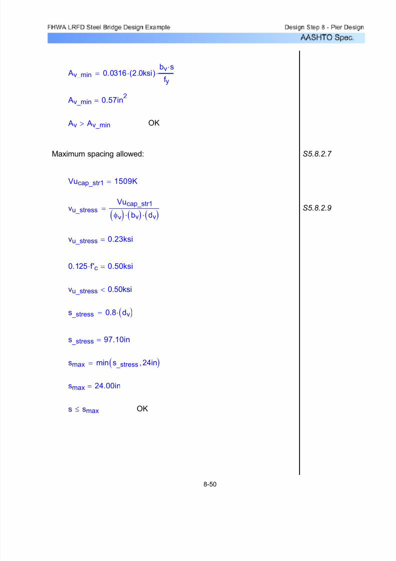
7/29/2019 LRFD steel design.pdf
http://slidepdf.com/reader/full/lrfd-steel-designpdf 512/646
OKs smax≤
smax 24.00in=
smax min s _stress 24in,( )=
s _stress 97.10in=
s _stress 0.8 dv( )⋅=
vu_stress 0.50ksi<
0.125 f'c⋅ 0.50ksi=
vu_stress 0.23ksi=
S5.8.2.9vu_stressVucap_str1
φv( ) bv( )⋅ dv( )⋅=
Vucap_str1 1509K=
S5.8.2.7 Maximum spacing allowed:
OK Av Av_min>
Av_min 0.57in2=
Av_min 0.0316 2.0ksi( )⋅bv s⋅
f y⋅=
8-50
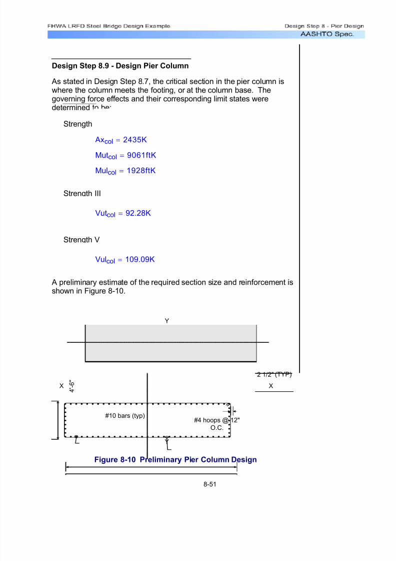
7/29/2019 LRFD steel design.pdf
http://slidepdf.com/reader/full/lrfd-steel-designpdf 513/646
Design Step 8.9 - Design Pier Column
As stated in Design Step 8.7, the critical section in the pier column iswhere the column meets the footing, or at the column base. The
governing force effects and their corresponding limit states weredetermined to be:
Strength I
Axcol 2435K=
Mutcol 9061ftK=
Mulcol 1928ftK=
Strength III
Vutcol 92.28K=
Strength V
Vulcol 109.09K=
A preliminary estimate of the required section size and reinforcement is
shown in Figure 8-10.
15'-6"
X X
Y
Y
2 1/2"
4 ' - 6 "
#4 hoops @ 12"
O.C.
#10 bars (typ)
(TYP)
Figure 8-10 Preliminary Pier Column Design
8-51

7/29/2019 LRFD steel design.pdf
http://slidepdf.com/reader/full/lrfd-steel-designpdf 514/646
For simplicity in the calculations that follow, let lu=lux=luy and Kcol=Kx=Ky.This is conservative for the transverse direction for this structure, andthe designer may select a lower value. The radius of gyration (r) abouteach axis can then be computed as follows:
CTable4.6.2.5-1
For this pier, the unbraced lengths (lux, luy) used in computing theslenderness ratio about each axis is the full pier height. This is theheight from the top of the footing to the top of the pier cap (26 feet). The
effective length factors, Kx and Ky, are both taken equal to 2.1. Thisassumes that the superstructure has no effect on restraining the pier from buckling. In essence, the pier is considered a free-standingcantilever.
S5.7.4.1
S5.7.4.3The column slenderness ratio (Klu/r) about each axis of the column iscomputed below in order to assess slenderness effects. Note that theSpecifications only permit the following approximate evaluation of slenderness effects when the slenderness ratio is below 100.
OK0.144 0.135≥ As_col f y⋅ Ag_col f c⋅
0.144=
OK0.0096 0.08≤ As_col
Ag_col0.0096=
Ag_col 10044in2=
Ag_col 4.5 ft⋅( ) 15.5 ft⋅( )⋅144 in2⋅
1ft2
⋅=
As_col 96.52in2=
As_col Num_bars( ) bar_area10( )⋅=
bar_area10 1.27in2=Num_bars 76=
S5.7.4.2 The preliminary column reinforcing is show in Figure 8-10 andcorresponds to #10 bars equally spaced around the column perimeter.
The Specifications prescribes limits (both maximum and minimum) onthe amount of reinforcing steel in a column. These checks areperformed on the preliminary column as follows:
S5.7.4Design for Axial Load and Biaxial Bending (Strength I):
8-52

7/29/2019 LRFD steel design.pdf
http://slidepdf.com/reader/full/lrfd-steel-designpdf 515/646
S5.7.4.3The Specifications permits slenderness effects to be ignored when theslenderness ratio is less than 22 for members not braced againstsidesway. It is assumed in this example that the pier is not bracedagainst sidesway in either its longitudinal or transverse directions.Therefore, slenderness will be considered for the pier longitudinaldirection only (i.e., about the "X-X" axis).
OK12.20 100<Kcol lu⋅( )
r yy
12.20=
OK42.03 100<Kcol lu⋅( )
r xx42.03=
lu 312in=Kcol 2.1=
The slenderness ratio for each axis now follows:
r yy 53.69in=
r yyIyy
Ag_col=
r xx 15.59in=
r xxIxx
Ag_col=
Iyy 28956852in4=Iyy 112
54in( )⋅ 186in( )3⋅=
Ixx 2440692in4=Ixx
1
12186in( )⋅ 54in( )
3⋅=
8-53
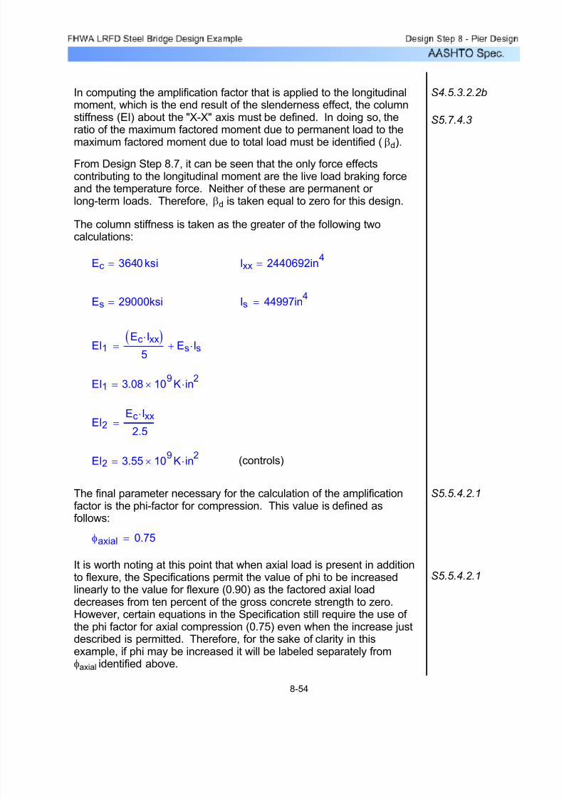
7/29/2019 LRFD steel design.pdf
http://slidepdf.com/reader/full/lrfd-steel-designpdf 516/646
S5.5.4.2.1It is worth noting at this point that when axial load is present in additionto flexure, the Specifications permit the value of phi to be increasedlinearly to the value for flexure (0.90) as the factored axial loaddecreases from ten percent of the gross concrete strength to zero.However, certain equations in the Specification still require the use of the phi factor for axial compression (0.75) even when the increase justdescribed is permitted. Therefore, for the sake of clarity in thisexample, if phi may be increased it will be labeled separately fromφaxial identified above.
φaxial 0.75=
S5.5.4.2.1The final parameter necessary for the calculation of the amplificationfactor is the phi-factor for compression. This value is defined asfollows:
(controls)EI2 3.55 109× K in
2⋅=
EI2 Ec Ixx⋅2.5
=
EI1 3.08 109× K in
2⋅=
EI1Ec Ixx⋅( )
5Es Is⋅+=
Is 44997in4=Es 29000ksi=
Ixx 2440692in4=Ec 3640 ksi=
The column stiffness is taken as the greater of the following twocalculations:
From Design Step 8.7, it can be seen that the only force effectscontributing to the longitudinal moment are the live load braking forceand the temperature force. Neither of these are permanent or long-term loads. Therefore, βd is taken equal to zero for this design.
S5.7.4.3
S4.5.3.2.2bIn computing the amplification factor that is applied to the longitudinalmoment, which is the end result of the slenderness effect, the columnstiffness (EI) about the "X-X" axis must be defined. In doing so, theratio of the maximum factored moment due to permanent load to the
maximum factored moment due to total load must be identified (βd).
8-54

7/29/2019 LRFD steel design.pdf
http://slidepdf.com/reader/full/lrfd-steel-designpdf 517/646
S5.7.4.5 The assessment of the resistance of a compression member withbiaxial flexure for strength limit states is dependent upon the magnitudeof the factored axial load. This value determines which of twoequations provided by the Specification are used.
Muy 9061ftK=Muy Mutcol=
Mux 2008ftK=Mux Mulcol δs⋅=
Pu_col 2435K=Pu_col Axcol=
The final design forces at the base of the column for the Strength I limitstate will be redefined as follows:
δs 1.04=δs 1
1 Axcol
φaxial Pe⋅
⎛
⎝
⎞
⎠−
=
Pe 81701K=Peπ
2EI2( )⋅
Kcol lu⋅( )2=
S4.5.3.2.2bThe longitudinal moment magnification factor will now be calculated asfollows:
φLow_axial 0.81=
φLow_axial 0.90 0.15 Axcol
0.10( )( ) f c( )⋅ Ag_col( )⋅
⎡
⎣
⎤
⎦⋅−=
Since the factored axial load in the column is less than ten percent of the gross concrete strength, the phi-factor will be modified andseparately labeled as follows:
0.10( ) f'c( )⋅ Ag_col( )⋅ 4018K=
Axcol 2435K=
8-55

7/29/2019 LRFD steel design.pdf
http://slidepdf.com/reader/full/lrfd-steel-designpdf 518/646
If the factored axial load is less than ten percent of the gross concretestrength multiplied by the phi-factor for compression members (φaxial),
then the Specifications require that a linear interaction equation for only
the moments is satisfied (SEquation 5.7.4.5-3). Otherwise, an axial
load resistance (Prxy) is computed based on the reciprocal load method(SEquation 5.7.4.5-1). In this method, axial resistances of the columnare computed (using φLow_axial if applicable) with each moment acting
separately (i.e., Prx with Mux, Pry with Muy). These are used along withthe theoretical maximum possible axial resistance (Po multiplied byφaxial) to obtain the factored axial resistance of the biaxially loaded
column.
Regardless of which of the two equations mentioned in the aboveparagraph controls, commercially available software is generally usedto obtain the moment and axial load resistances.
For this pier design, the procedure as discussed above is carried outas follows:
0.10( ) φaxial( )⋅ f'c( )⋅ Ag_col( )⋅ 3013K=
Pu_col 3013K<
Therefore, SEquation 5.7.4.5-3 will be used.
Mux 2008ftK= Muy 9061ftK=
Mrx 10440ft K⋅= Mry 36113ft K⋅=
Mux
Mrx
Muy
Mry+ 0.44= 0.44 1.0≤ OK
The factored flexural resistances shown above, Mrx and Mry, wereobtained by the use of commercial software. These values are theflexural capacities about each respective axis assuming that no axialload is present. Consistent with this, the phi-factor for flexure (0.90)was used in obtaining the factored resistance from the factorednominal strength.
Although the column has a fairly large excess flexural capacity, a moreoptimal design will not be pursued per the discussion following thecolumn shear check.
8-56

7/29/2019 LRFD steel design.pdf
http://slidepdf.com/reader/full/lrfd-steel-designpdf 519/646
Vc 914.08K=
S5.8.3.3Vc 0.0316 β⋅ 2ksi( )⋅ bv⋅ dv⋅=
4 1 ksi⋅( ) 2.00ksi=
The nominal concrete shear strength is:
S5.8.3.4.1θ 45deg=β 2.0=
The above calculation for dv is simple to use for columns and generallyresults in a conservative estimate of the shear capacity.
dv 133.92in=
S5.8.2.9dv 0.72( ) h( )⋅=
S5.8.3.3h 186 in⋅=bv 54.in=
S5.8.2.4
For the pier column of this example, the maximum factored shear ineither direction is less than one-half of the factored resistance of theconcrete. Therefore, shear reinforcement is not required. This isdemonstrated for the transverse direction as follows:
These maximum shear forces do not act concurrently. Although afactored longitudinal shear force is present in Strength III and a factoredtransverse shear force is present in Strength V, they both are smallrelative to their concurrent factored shear. Therefore, separate shear designs can be carried out for the longitudinal and transverse directions
using only the maximum shear force in that direction.
(Strength V)Vulcol 109.09K=
(Strength III)Vutcol 92.28K=
The maximum factored transverse and longitudinal shear forces werederived in Design Step 8.7 and are as follows:
S5.8 Design for Shear (Strength III and Strength V)
8-57
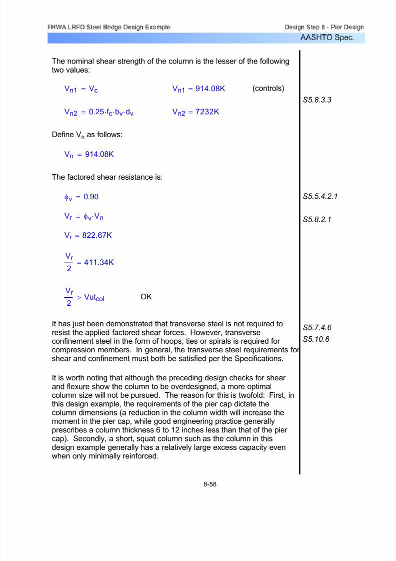
7/29/2019 LRFD steel design.pdf
http://slidepdf.com/reader/full/lrfd-steel-designpdf 520/646
It is worth noting that although the preceding design checks for shear and flexure show the column to be overdesigned, a more optimal
column size will not be pursued. The reason for this is twofold: First, inthis design example, the requirements of the pier cap dictate thecolumn dimensions (a reduction in the column width will increase themoment in the pier cap, while good engineering practice generallyprescribes a column thickness 6 to 12 inches less than that of the pier cap). Secondly, a short, squat column such as the column in thisdesign example generally has a relatively large excess capacity evenwhen only minimally reinforced.
S5.10.6
S5.7.4.6 It has just been demonstrated that transverse steel is not required toresist the applied factored shear forces. However, transverseconfinement steel in the form of hoops, ties or spirals is required for compression members. In general, the transverse steel requirements for shear and confinement must both be satisfied per the Specifications.
OKVr 2
Vutcol>
Vr
2411.34K=
Vr 822.67K=
S5.8.2.1Vr φv Vn⋅=
S5.5.4.2.1φv 0.90=
The factored shear resistance is:
Vn 914.08K=
Define Vn as follows:
Vn2 7232K=Vn2 0.25 f c⋅ bv⋅ dv⋅=S5.8.3.3
(controls)Vn1 914.08K=Vn1 Vc=
The nominal shear strength of the column is the lesser of the followingtwo values:
8-58
7/29/2019 LRFD steel design.pdf
http://slidepdf.com/reader/full/lrfd-steel-designpdf 521/646
S5.5.4.2.1 φv 0.90=
f'c 4.0ksi=f y 60ksi=
µ 1.00=µ 1.0 λ⋅=
S5.8.4.2 λ 1.00=ccv 0.100ksi=
Avf 96.52in2= Avf As_col=
S5.8.4.1 Acv 10044in2= Acv Ag_col=
In addition to the above, the Specifications requires that the transfer of lateral forces from the pier to the footing be in accordance with the
shear-transfer provisions of S5.8.4. With the standard detailingpractices for bridge piers previously mentioned (i.e., all columnreinforcement extended and developed in the footing), along withidentical design compressive strengths for the column and footing, thisrequirement is generally satisfied. However, for the sake of
completeness, this check will be carried out as follows:
In this design example, and consistent with standard engineeringpractice, all steel reinforcing bars in the column extend into, and aredeveloped, in the footing (see Figure 8-13). This automaticallysatisfies the following requirements for reinforcement across theinterface of the column and footing: A minimum reinforcement areaof 0.5 percent of the gross area of the supported member, aminimum of four bars, and any tensile force must be resisted by the
reinforcement. Additionally, with all of the column reinforcementextended into the footing, along with the fact that the column andfooting have the same compressive strength, a bearing check at thebase of the column and the top of the footing is not applicable.
The provisions for the transfer of forces and moments from thecolumn to the footing are new to the AASHTO LRFD Specifications.
Although similar provisions have existed in the ACI Building Code for some time, these provisions are absent from the AASHTO StandardSpecifications. In general, standard engineering practice for bridgepiers automatically satisfies most, if not all, of these requirements.
S5.13.3.8 Transfer of Force at Base of Column
8-59

7/29/2019 LRFD steel design.pdf
http://slidepdf.com/reader/full/lrfd-steel-designpdf 522/646
Transfer of Force at Column Base
For common bridges with standard detailing of bridgepiers and the same design compressive strength of the column and the footing, S5.13.3.8 can beconsidered satisfied.
As can be seen, a large excess capacity exists for this check. This ispartially due to the fact that the column itself is overdesigned in general(this was discussed previously). However, the horizontal forcesgenerally encountered with common bridges are typically small relativeto the shear-friction capacity of the column (assuming all reinforcingbars are extended into the footing). In addition, the presence of ashear-key, along with the permanent axial compression from thebridge dead load, further increase the shear-friction capacity at thecolumn/footing interface beyond that shown above. This may accountfor the absence of this check in both the Standard Specifications andin standard practice.
OKφv Vnsf ( )⋅ Vulcol≥
φv Vnsf ( )⋅ 6116K=
It then follows:
Vulcol 109.09K=
The maximum applied shear was previously identified from the StrengthV limit state:
Vnsf 6796K=Vnsf Vnsf1=
Define the nominal shear-friction capacity as follows:
Vnsf3 8035K=Vnsf3 0.8 Acv⋅ 1 ksi⋅( )⋅=
Vnsf2 8035K=Vnsf2 0.2 f'c⋅ Acv⋅=
Vnsf1 6796K=Vnsf1 ccv Acv⋅ µ Avf ⋅ f y⋅+=
S5.8.4.1The nominal shear-friction capacity is the smallest of the following threeequations (conservatively ignore permanent axial compression):
8-60
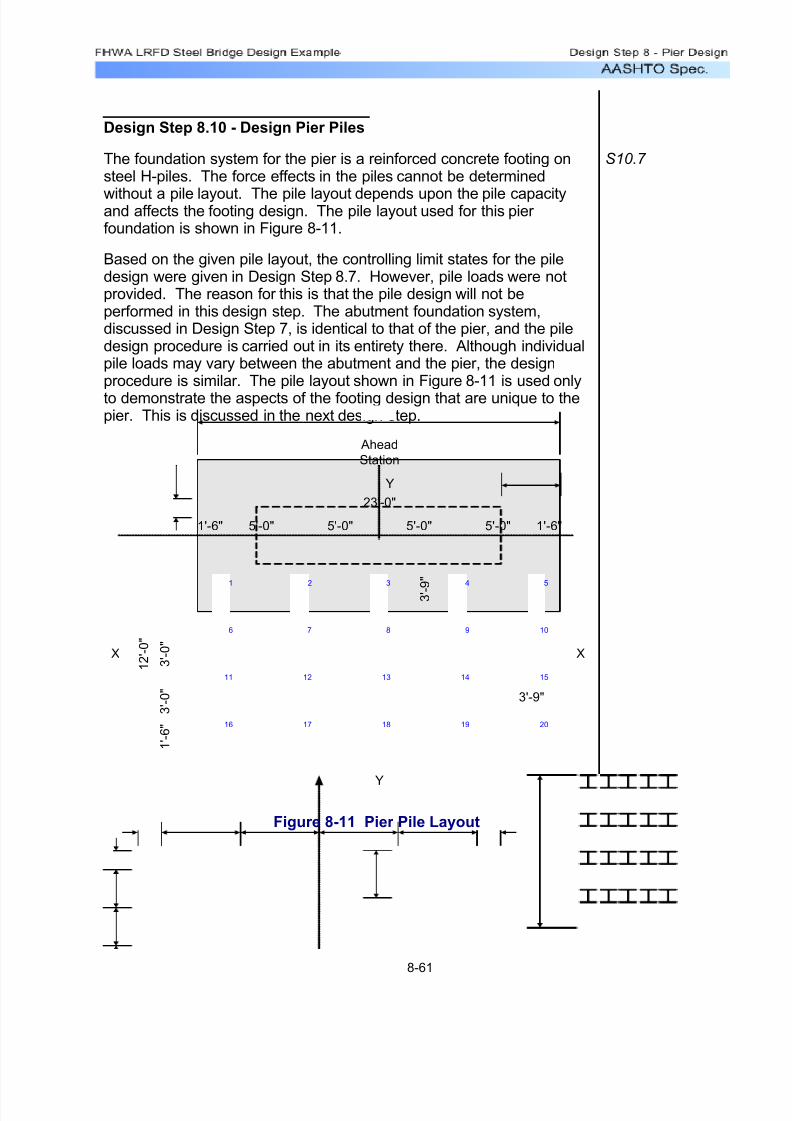
7/29/2019 LRFD steel design.pdf
http://slidepdf.com/reader/full/lrfd-steel-designpdf 523/646
Design Step 8.10 - Design Pier Piles
The foundation system for the pier is a reinforced concrete footing onsteel H-piles. The force effects in the piles cannot be determined
without a pile layout. The pile layout depends upon the pile capacityand affects the footing design. The pile layout used for this pier foundation is shown in Figure 8-11.
S10.7
Based on the given pile layout, the controlling limit states for the piledesign were given in Design Step 8.7. However, pile loads were notprovided. The reason for this is that the pile design will not beperformed in this design step. The abutment foundation system,discussed in Design Step 7, is identical to that of the pier, and the piledesign procedure is carried out in its entirety there. Although individualpile loads may vary between the abutment and the pier, the designprocedure is similar. The pile layout shown in Figure 8-11 is used onlyto demonstrate the aspects of the footing design that are unique to thepier. This is discussed in the next design step.
23'-0"
X X
Y
Y
1'-6" 5'-0" 5'-0" 5'-0" 5'-0" 1'-6"
1 ' - 6 "
3 ' - 0 "
3 ' - 0 "
3 ' - 0 "
1 ' - 6 "
3 ' - 9 "
3'-9"
Ahead
Station
1 2 ' - 0 "
16
11
6
1
17
12
7
2
18
13
8
3
19
14
9
4
20
15
10
5
Figure 8-11 Pier Pile Layout
8-61

7/29/2019 LRFD steel design.pdf
http://slidepdf.com/reader/full/lrfd-steel-designpdf 524/646
Design Step 8.11 - Design Pier Footing
In Design Step 8.7, the governing limit states were identified for thedesign of the pier footing. However, the factored force effects were
only given for the Strength I check of punching shear at the column.The reason for this is that most of the design checks for the pier footing are performed similarly to those of the abutment footing inDesign Step 7. Therefore, only the aspects of the footing design thatare unique to the pier footing will be discussed in this design step.This includes the punching (or two-way) shear check at the columnand a brief discussion regarding estimating the applied factoredshear and moment per foot width of the footing when adjacent pileloads differ.
The factored force effects from Design Step 8.7 for the punching shear check at the column are:
Axcol_punch 3583K=
Mutcol_punch 5287ft K⋅=
Mulcol_punch 2756ft K⋅=
It should be noted that in Design Step 8.5, the live load reactions at thebearings include dynamic load allowance on the truck loads. Theselive load force effects are part of the factored axial load and transverse
moment shown above. However, the Specifications do not requiredynamic load allowance for foundation components that are entirelybelow ground level. Therefore, the resulting pile loads will besomewhat larger (by about four percent) than necessary for thefollowing design check. For the sake of clarity and simplicity in DesignStep 8.5, a separate set of live load reactions with dynamic loadallowance excluded was not provided.
S3.6.2.1
The longitudinal moment given above must be magnified to account for slenderness of the column (see Design Step 8.9). The computedmagnification factor and final factored forces are:
δs_punch 1.06=
Pu_punch Axcol_punch= Pu_punch 3583K=
Mux_punch Mulcol_punch( ) δs_punch( )⋅=
Mux_punch 2921ftK=
8-62
see page -
7/29/2019 LRFD steel design.pdf
http://slidepdf.com/reader/full/lrfd-steel-designpdf 525/646
dex 37.31in=
dex 42in Cover ftg− bar_diam9−bar_diam9
2−=
dey 38.44in=
dey 42in Cover ftg−bar_diam9
2−=
Cover ftg 3in=
Effective depth for each axis:
(per foot width) As_ftg 2.00in2=
As_ftg 2 bar_area9( )⋅=
hftg 42in=bftg 12in=
bar_diam9 1.128in=bar_area9 1.00in2=
S5.13.3.6.3The effective shear depth, dv, must be defined in order to determine bo and the punching (or two-way) shear resistance. Actually, an averageeffective shear depth should be used since the two-way shear areaincludes both the "X-X" and "Y-Y" sides of the footing. In other words,dex is not equal to dey, therefore dvx will not be equal to dvy. This is
illustrated as follows assuming a 3'-6" footing with #9 reinforcing bars at6" on center in both directions in the bottom of the footing:
S5.13.3.6.1With the applied factored loads determined, the next step in the column
punching shear check is to define the critical perimeter, bo. TheSpecifications require that this perimeter be minimized, but need notbe closer than dv/2 to the perimeter of the concentrated load area. Inthis case, the concentrated load area is the area of the column on thefooting as seen in plan.
Muy_punch 5287ftK=Muy_punch Mutcol_punch=
8-63

7/29/2019 LRFD steel design.pdf
http://slidepdf.com/reader/full/lrfd-steel-designpdf 526/646
tcol 54in=bcol 186in=
With the average effective shear depth determined, the criticalperimeter can be calculated as follows:
dv_avg 36.40in=
dv_avgdvx dvy+( )
2=
Average effective shear depth:
dvy 36.97in=
S5.8.2.9dvy max deyaftg
2− 0.9 dey⋅, 0.72 hftg⋅,
⎛ ⎝
⎞ ⎠
=
dvx 35.84in=
S5.8.2.9dvx max dexaftg
2− 0.9 dex⋅, 0.72 hftg⋅,
⎛ ⎝
⎞ ⎠
=
aftg 2.94in=
aftgTftg
0.85 f c⋅ bftg⋅=
Tftg 120.00K=
Tftg As_ftg f y⋅=
Effective shear depth for each axis:
8-64
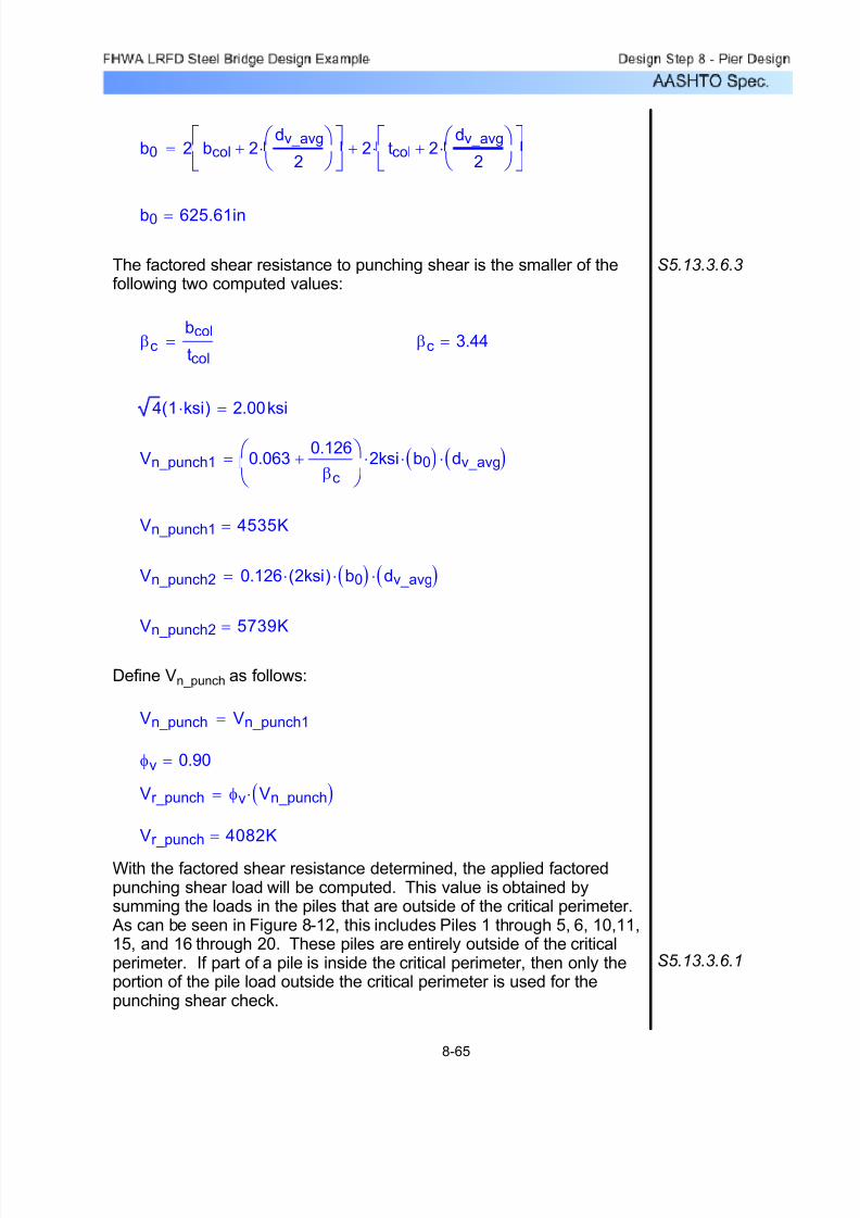
7/29/2019 LRFD steel design.pdf
http://slidepdf.com/reader/full/lrfd-steel-designpdf 527/646
S5.13.3.6.1
With the factored shear resistance determined, the applied factoredpunching shear load will be computed. This value is obtained bysumming the loads in the piles that are outside of the critical perimeter.
As can be seen in Figure 8-12, this includes Piles 1 through 5, 6, 10,11,15, and 16 through 20. These piles are entirely outside of the criticalperimeter. If part of a pile is inside the critical perimeter, then only theportion of the pile load outside the critical perimeter is used for thepunching shear check.
Vr_punch 4082K=
Vr_punch φv Vn_punch( )⋅=
φv 0.90=
Vn_punch Vn_punch1=
Define Vn_punch as follows:
Vn_punch2 5739K=
Vn_punch2 0.126 2ksi( )⋅ b0( )⋅ dv_avg( )⋅=
Vn_punch1 4535K=
Vn_punch1 0.0630.126
βc
+⎛
⎝
⎞
⎠2⋅ ksi b0( )⋅ dv_avg( )⋅=
4 1 ksi⋅( ) 2.00ksi=
βc 3.44=βc
bcol
tcol=
S5.13.3.6.3 The factored shear resistance to punching shear is the smaller of thefollowing two computed values:
b0 625.61in=
b0 2 bcol 2dv_avg
2
⎛ ⎝
⎞ ⎠
⋅+⎡⎣
⎤⎦
2 tcol 2dv_avg
2
⎛ ⎝
⎞ ⎠
⋅+⎡⎣
⎤⎦
⋅+=
8-65

7/29/2019 LRFD steel design.pdf
http://slidepdf.com/reader/full/lrfd-steel-designpdf 528/646
X X
Y
Y
Critical Perimeter
for Column
Punching Shear
ColumnPerimeter
+Mux
+Muy
d v
/ 2
16
11
6
1
17
12
7
2
18
13
8
3
19
14
9
4
20
15
10
5
Figure 8-12 Critical Perimeter for Column Punching Shear
The following properties of the pile group are needed to determine thepile loads (reference Figures 8-11 and 8-12):
npiles 20=
Ip_xx 5 1.5ft( )2
4.5ft( )2+⋅ 2⋅=
Ip_xx 225ft2=
Ip_yy 4 5 ft⋅( )2
10 ft⋅( )2+⋅ 2⋅=
Ip_yy 1000ft2=
The following illustrates the pile load in Pile 1:
P1Pu_punch
npiles
Mux_punch 4.5ft( )⋅
Ip_xx+
Muy_punch 10ft( )⋅
Ip_yy+=
P1 290.45K=
8-66

7/29/2019 LRFD steel design.pdf
http://slidepdf.com/reader/full/lrfd-steel-designpdf 529/646
Vu_punch_altPu_punch
npiles
⎛
⎝
⎞
⎠14⋅=
Alternate Punching Shear Load Calculation
An alternate method for carrying out the columnpunching shear check is to simply use the appliedfactored axial load to obtain equal pile loads in all of the piles. This is only valid for the case where the pilesoutside of the critical perimeter are symmetric about
both axes. The applied factored shear on the criticalsection is obtained as above (i.e., the sum of the pileslocated outside of the critical perimeter). Thisapproach yields the same value for Vu_punch as was
derived above. This is illustrated as follows:
OKVu_punch Vr_punch≤
Vu_punch 2509K=
Vu_punch P1 P2+ P3+ P4+ P5+ P6+ P10+P11 P15+ P16+ P17+ P18+ P19+ P20++
...=
The total applied factored shear used for the punching shear check is:
P20 68.40K=
P19 94.84K=P18 121.27K=
P17 147.71K=P16 174.14K=
P15 106.99K=P11 212.73K=
P10 145.57K=P6 251.31K=
P5 184.16K=P4 210.6K=
P3 237.03K=P2 263.47K=
Similar calculations for the other piles outside of the critical perimeter yield the following:
8-67

7/29/2019 LRFD steel design.pdf
http://slidepdf.com/reader/full/lrfd-steel-designpdf 530/646
Vu_punch_alt 2508K=
Vu_punch_alt Vu_punch=
It has just been shown that the factored axial load alone is sufficient for the punching shear check at the column. However, consideration of thefactored axial load along with the corresponding applied factoredmoments is necessary for other footing design checks such aspunching shear at the maximum loaded pile, one-way shear, andflexure. This applies to the abutment footing in Design Step 7 as well.However, what is unique to the pier footing is that significant momentsact about both axes. What follows is a demonstration, using the pileforces previously computed, of an estimation of the applied factoredload on a per-foot basis acting on each footing face. The following
estimations are based on the outer row of piles in each direction,respectively. Once these estimates are obtained, the appropriatefooting design checks are the same as those for the abutment footing.
Lftg_xx 23ft= Lftg_yy 12ft=
Estimation of applied factored load per foot in the "X" direction:
Restimate_xx2 P1 P2+( )⋅ P3+
Lftg_xx
=
Restimate_xx 58.47K
ft=
Estimation of applied factored load per foot in the "Y" direction:
Restimate_yy2 P1 P6+( )⋅
Lftg_yy=
Restimate_yy 90.29K
ft=
8-68

7/29/2019 LRFD steel design.pdf
http://slidepdf.com/reader/full/lrfd-steel-designpdf 531/646
Design Step 8.12 - Final Pier Schematic
Figure 8-13 shows the final pier dimensions along with the requiredreinforcement in the pier cap and column.
5 ' - 0 "
6 ' - 0 "
15'-0"
46'-6"
3'-6"
23'-0"
#5 hoops @ 9" spacing
2 rows of
10 - #11 bars
76 - #10 bars equally
spaced around
column perimeter
# 4 h o o p s @ 1
2 "
s p a c i n g ( t y p )
15'-6"
#8 bars
@ 12"
spacing
#8bars@
8"sp
acing
Figure 8-13 Final Pier Design
8-69

7/29/2019 LRFD steel design.pdf
http://slidepdf.com/reader/full/lrfd-steel-designpdf 532/646
36
Design Step P.9 - Determine Factored Axial Geotechnical
Resistance for Single Pile
37
Design Step P.10 - Check Drivability of Pile 38
Design Step P.11 - Do Preliminary Pile Layout Based onFactored Loads and Overturning Moments
53
Design Step P.12 - Evaluate Pile Head Fixity 63
Design Step P.13 - Perform Pile Soil Interaction Analysis 65
Design Step P.14 - Check Geotechnical Axial Capacity 77
Design Step P.15 - Check Structural Axial Capacity(in lower portion of pile)
78
Design Step P.16 - Check Structural Axial Capacity inCombined Bending and Axial Load(upper portion of pile)
79
Design Step P.17 - Check Structural Shear Capacity 89
Pile Foundation Design ExampleDesign Step P
Table of Contents Page
Design Step P.1 - Define Subsurface Conditions and AnyGeometric Constraints
2
Design Step P.2 - Determine Applicable Loads and LoadCombinations
13
Design Step P.3 - Factor Loads for Each Combination 14
Design Step P.4 - Verify Need for a Pile Foundation 16
Design Step P.5 - Select Suitable Pile Type and Size 23
Design Step P.6 - Determine Nominal Axial StructuralResistance for Selected Pile Type / Size
32
Design Step P.7 - Determine Nominal Axial GeotechnicalResistance for Selected Pile Type / Size
33
Design Step P.8 - Determine Factored Axial StructuralResistance for Single Pile
P-1

7/29/2019 LRFD steel design.pdf
http://slidepdf.com/reader/full/lrfd-steel-designpdf 533/646
PSFlb
ft2
=psilb
in2
=K 1000 lb⋅=KSF1000 lb⋅
ft2
=
kilo 1000=TSFton
ft2
=ksi1000 lb⋅
in2
=PCFlb
ft3
=
The following units are defined for use in this design example:
Refer to Design Step 1 for introductory information about this designexample. Additional information is presented about the designassumptions, methodology, and criteria for the entire bridge, includingthe Pile Foundation Design.
For Abutment 1, one boring was drilled at each side of the abutment.These borings are illustrated graphically in Section A1 below.
A subsurface investigation was conducted at the site. Two testborings were drilled at each substructure unit. Soils were sampled at3 foot intervals using a split spoon sampler in accordance with ASTMD-1586. Rock was continuously sampled with an N series core barrelin accordance with ASTM D-2113.
This task involves determining the location and extent of soil and rockmaterials beneath the proposed abutment and determiningengineering design properties for each of those materials. It alsoincludes identification of any specific subsurface conditions that mayimpact the performance of the structure. The design of the foundationsystem needs to address any identified issues.
Design Step P.1 - Define Subsurface Conditions and Any
Geometric Constraints
103References
92Design Step P.19 - Additional Miscellaneous Design Issues
91Design Step P.18 - Check Maximum Horizontal and VerticalDeflection of Pile Group at Beam Seats UsingService Load Case
P-2
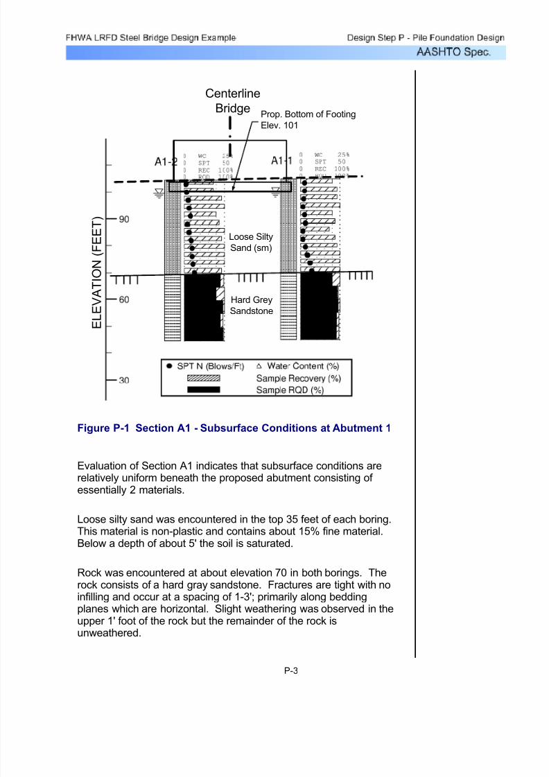
7/29/2019 LRFD steel design.pdf
http://slidepdf.com/reader/full/lrfd-steel-designpdf 534/646
E L E V A T I O
N ( F E E T )
Centerline
BridgeProp. Bottom of Footing
Elev. 101
Loose Silty
Sand (sm)
Hard Grey
Sandstone
Figure P-1 Section A1 - Subsurface Conditions at Abutment 1
Evaluation of Section A1 indicates that subsurface conditions arerelatively uniform beneath the proposed abutment consisting of essentially 2 materials.
Loose silty sand was encountered in the top 35 feet of each boring.This material is non-plastic and contains about 15% fine material.
Below a depth of about 5' the soil is saturated.
Rock was encountered at about elevation 70 in both borings. Therock consists of a hard gray sandstone. Fractures are tight with noinfilling and occur at a spacing of 1-3'; primarily along beddingplanes which are horizontal. Slight weathering was observed in theupper 1' foot of the rock but the remainder of the rock isunweathered.
P-3

7/29/2019 LRFD steel design.pdf
http://slidepdf.com/reader/full/lrfd-steel-designpdf 535/646
Special Geotechnical Considerations:
The loose fine sandy soils could be subject to liquefaction under
seismic loading. Liquefaction is a function of the anticipatedmaximum earthquake magnitude and the soil properties. If liquefaction is a problem, the soils can not be relied upon toprovide lateral support to deep foundation systems. For thisexample it is assumed that the potential for liquefaction has beenevaluated and has been found to be negligible. (Note: Seed andIdriss (NCEER-97-0022) provides more up to date material for evaluation of liquefaction)
C10.5.4,
SAppendix A10
The weight of the approach embankment will cause compression
of the loose soil horizon. The granular material should compressessentially elastically with little or no long term consolidation.However, since the full height abutment will likely be placed prior to completion of the approach embankment in the vicinity of theabutment, soil compression beneath the abutment must beaccounted for in foundation design. For shallow foundations, thiscompression will result in settlement and rotation of the footing.For deep foundations this compression could result in negativeskin friction (downdrag) loads on the foundation elements;particularly in the back row of piles.
S10.7.1.4,
C10.7.1.4
P-4

7/29/2019 LRFD steel design.pdf
http://slidepdf.com/reader/full/lrfd-steel-designpdf 536/646
Υeff 47.6PCF=
Υeff Υwet Υwater −=Effective unit weight:
Υwater 62.4 PCF⋅=Unit weight of water:
Υwet 110 PCF⋅=Wet unit weight:
Υdry 90 PCF⋅=Dry unit weight:
C10.4.1Consider relevant published data when selecting design
parameters. For unit weights of in-situ soil materials, agood reference is NAVFAC DM7.1-22. Based on thisreference, general and local experience, and the abovedescription of the soil horizon as loose silty sand, theunit weights were selected as follows:
Unit Weight (Υ):
101 ft⋅ 70 ft⋅− 31ft=
Assuming a bottom of footing elevation of 101 FT anda top of rock elevation of 70 FT as described above:
Depth:
Layer 1 - Soil
Development of Parameters for Design:
P-5
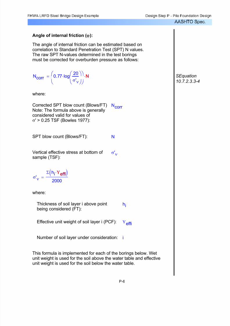
7/29/2019 LRFD steel design.pdf
http://slidepdf.com/reader/full/lrfd-steel-designpdf 537/646
This formula is implemented for each of the borings below. Wetunit weight is used for the soil above the water table and effectiveunit weight is used for the soil below the water table.
iNumber of soil layer under consideration:
ΥeffiEffective unit weight of soil layer i (PCF):
hiThickness of soil layer i above pointbeing considered (FT):
where:
σ'νΣ hi Υeffi⋅( )
2000=
Υeffi
σ'νVertical effective stress at bottom of sample (TSF):
NSPT blow count (Blows/FT):
Ncorr Corrected SPT blow count (Blows/FT)Note: The formula above is generally
considered valid for values of σ' > 0.25 TSF (Bowles 1977):
where:
SEquation
10.7.2.3.3-4Ncorr 0.77 log
20
σ'ν
⎛
⎝
⎞
⎠⋅⎛
⎝
⎞
⎠N⋅= N
The angle of internal friction can be estimated based oncorrelation to Standard Penetration Test (SPT) N values.The raw SPT N-values determined in the test boringsmust be corrected for overburden pressure as follows:
Angle of internal friction (ϕ):
P-6

7/29/2019 LRFD steel design.pdf
http://slidepdf.com/reader/full/lrfd-steel-designpdf 538/646
Depth to
Top of
Sample (FT)
Depth to
Bottom of
Sample (FT)
Υeff i
(PCF)σν' (TSF)
N
Blows/Ft
(BPF)
Ncorr
Blows/Ft
(BPF)
0 1.5 110 0.0825 5 93 4.5 110 0.2475 5 7
6 7.5 47.6 0.3189 4 6
9 10.5 47.6 0.3903 3 4
12 13.5 47.6 0.4617 5 6
15 16.5 47.6 0.5331 6 7
18 19.5 47.6 0.6045 3 4
21 22.5 47.6 0.6759 3 3
24 25.5 47.6 0.7473 6 7
27 28.5 47.6 0.8187 9 10
30 31.5 47.6 0.8901 12 12
33 34.5 47.6 0.9615 14 14
0 1.5 110 0.0825 2 4
3 4.5 110 0.2475 3 4
6 7.5 47.6 0.3189 5 7
9 10.5 47.6 0.3903 6 8
12 13.5 47.6 0.4617 8 10
15 16.5 47.6 0.5331 4 5
18 19.5 47.6 0.6045 6 7
21 22.5 47.6 0.6759 9 10
24 25.5 47.6 0.7473 10 11
27 28.5 47.6 0.8187 10 11
30 31.5 47.6 0.8901 11 11
33 34.5 47.6 0.9615 13 13
Boring A1-2
Boring A1-1
Table P-1 Calculation of Corrected SPT Blow Count
Find average values for zone between bottom of footing and top of rock. This means ignoring the first two values of each boring.
N 7.35= BPF
Ncorr 8.3= BPF
P-7
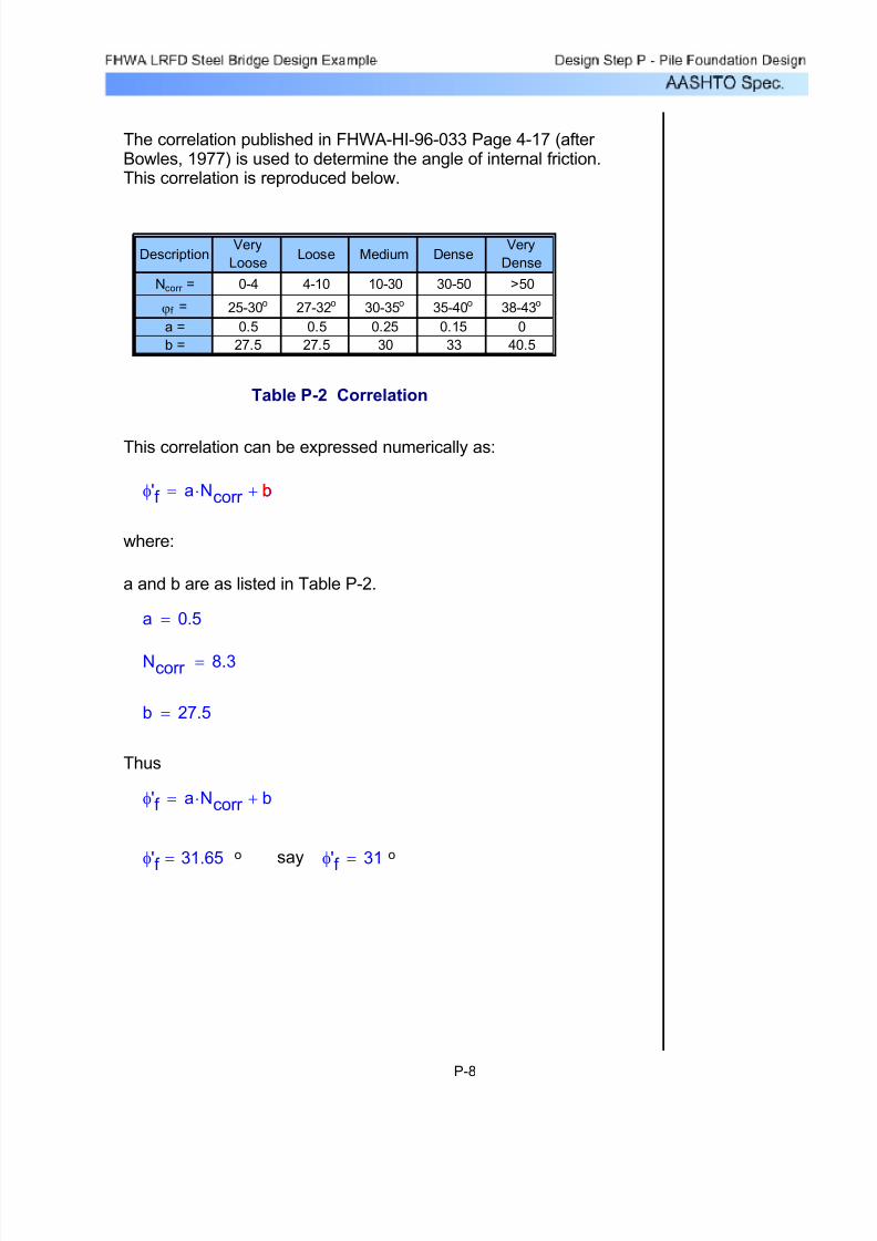
7/29/2019 LRFD steel design.pdf
http://slidepdf.com/reader/full/lrfd-steel-designpdf 539/646
oφ'f
31=sayoφ'f
31.65=
φ'f a Ncorr ⋅ b+=
Thus
b 27.5=
Ncorr 8.3=
a 0.5=
a and b are as listed in Table P-2.
where:
φ'f a Ncorr ⋅ b+= b
This correlation can be expressed numerically as:
Table P-2 Correlation
DescriptionVery
LooseLoose Medium Dense
Very
Dense
Ncorr = 0-4 4-10 10-30 30-50 >50
ϕf = 25-30o 27-32o 30-35o 35-40o 38-43o
a = 0.5 0.5 0.25 0.15 0
b = 27.5 27.5 30 33 40.5
The correlation published in FHWA-HI-96-033 Page 4-17 (after Bowles, 1977) is used to determine the angle of internal friction.This correlation is reproduced below.
P-8

7/29/2019 LRFD steel design.pdf
http://slidepdf.com/reader/full/lrfd-steel-designpdf 540/646
G0 0.33ksi=
G0 24TSF=
G0
E0
2 1 ν+( )⋅=
From Elastic Theory:
Shear Modulus (G):
ν 0.25=Loose Fine Sand:
STable
10.6.2.2.3b-1
Estimating ν from description
Poisons Ratio (ν):
E0 0.833ksi=
E0 60 TSF⋅=
Based on above, use:
TSFE0 58.1=
E0 7 Ncorr ⋅=
STable
10.6.2.2.3b-1E0 7 N1⋅= N1
Clean fine to medium sands and slightly silty sands
Note, in Table 10.6.2.2.3b-1 N1 is equivalent to Ncorr
Estimating E0 from Ncorr
80 - 120 TSFLoose Fine Sand E0 =
STable
10.6.2.2.3b-1
Estimating E0 from description
Modulus of elasticity (E):
P-9
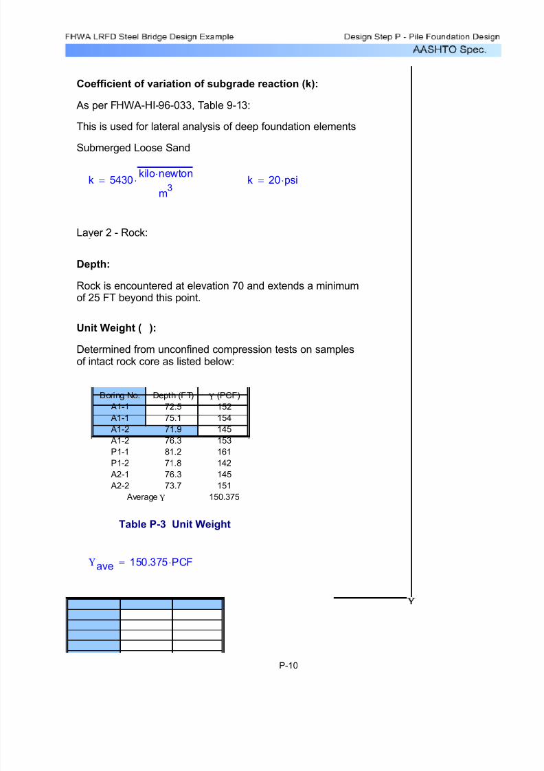
7/29/2019 LRFD steel design.pdf
http://slidepdf.com/reader/full/lrfd-steel-designpdf 541/646
Coefficient of variation of subgrade reaction (k):
As per FHWA-HI-96-033, Table 9-13:
This is used for lateral analysis of deep foundation elements
Submerged Loose Sand
k 5430kilo newton⋅
m3
⋅= k 20 psi⋅=
Layer 2 - Rock:
Depth:
Rock is encountered at elevation 70 and extends a minimumof 25 FT beyond this point.
Unit Weight (Υ):
Determined from unconfined compression tests on samplesof intact rock core as listed below:
Boring No. Depth (FT) Υ (PCF)
A1-1 72.5 152 A1-1 75.1 154
A1-2 71.9 145
A1-2 76.3 153
P1-1 81.2 161
P1-2 71.8 142
A2-1 76.3 145
A2-2 73.7 151
150.375 Average Υ
Table P-3 Unit Weight
Υave 150.375 PCF⋅=
P-10

7/29/2019 LRFD steel design.pdf
http://slidepdf.com/reader/full/lrfd-steel-designpdf 542/646
νave 0.2=For sandstone, Average:
This is to be used for prediction of pile tip response
STable
10.6.2.2.3d-1
Poisons Ratio (ν):
E0 2125ksi=
E0 153000 TSF⋅=For sandstone, Average:
This is to be used for prediction of deep foundation response
STable
10.6.2.2.3d-2
Modulus of elasticity (E):
quave 11485 psi⋅=
Table P-4 Unconfined Compressive
Strength
Boring No. Depth (FT) qu (PSI)
A1-1 72.5 12930
A1-1 75.1 10450
A1-2 71.9 6450
A1-2 76.3 12980
P1-1 81.2 14060
P1-2 71.8 6700
A2-1 76.3 13420
A2-2 73.7 1489011485 Average qu
Determined from unconfined compression tests on samplesof intact rock core as listed below:
Unconfined Compressive Strength (q):
P-11

7/29/2019 LRFD steel design.pdf
http://slidepdf.com/reader/full/lrfd-steel-designpdf 543/646
Shear Modulus (G):
From elastic theory
G0E0
2 1 νave+( )⋅=
G0 63750TSF=
G0 885.417ksi=
Rock Mass Quality:
Rock mass quality is used to correct the intact rock strength andintact modulus values for the effects of existing discontinuities inthe rock mass. This is done through empirical correlations usingparameters determined during core drilling.
Data from the test borings is summarized below:
Depth
(FT)
Run
Length
(FT)
Recovery
(%)RQD (%)
35 5 100 80
40 5 96 94
45 5 100 96
50 5 98 92
55 5 98 90
35 5 98 90
40 5 100 80
45 5 100 96
50 5 96 90
55 5 98 96
98.4 90.4
Boring A1-1
Boring A1-2
Averages
Table P-5 Rock Mass Quality
P-12

7/29/2019 LRFD steel design.pdf
http://slidepdf.com/reader/full/lrfd-steel-designpdf 544/646
Design Step P.2 - Determine Applicable Loads and Load
Combinations
Loads and load combinations are determined elsewhere in thedesign process. The critical load cases for evaluation of foundation design are summarized below:
1). The load combination that produces the maximum vertical loadon the foundation system. This will typically be a Strength I anda Service I load case with the maximum load factors applied.
2). The load combination that produces the maximum overturningon the foundation which will tend to lift a spread footing off thebearing stratum or place deep foundation elements in tension.
3). The load combination that produces the maximum lateral load.If several combinations produce the same horizontal load,select the one with the minimum vertical load as this will becritical for evaluation of spread footing sliding or response of battered deep foundations. In some cases, particularly deepfoundations employing all vertical elements, the highest lateralload and associated highest vertical load should also beevaluated as this case may produce higher foundationelement stress and deflections due to combined axial loadand bending in the foundation elements.
P-13
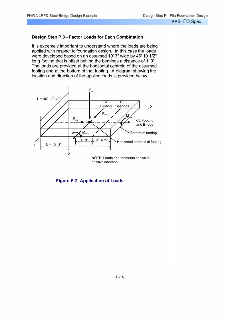
7/29/2019 LRFD steel design.pdf
http://slidepdf.com/reader/full/lrfd-steel-designpdf 545/646
Design Step P.3 - Factor Loads for Each Combination
It is extremely important to understand where the loads are beingapplied with respect to foundation design. In this case the loads
were developed based on an assumed 10' 3" wide by 46' 10 1/2"long footing that is offset behind the bearings a distance of 1' 9".The loads are provided at the horizontal centroid of the assumedfooting and at the bottom of that footing. A diagram showing thelocation and direction of the applied loads is provided below.
X
Z
Y
P
M
MP
P
vert
trans
long
long
trans
CL
Footing
CL
Bearings
CL Footing
and Bridge
Bottom of footing
Horizontal centroid of footing
NOTE: Loads and moments shown in
positive direction
L = 46' 10 ½"
B = 10' 3"
1' 9" 3' 4 ½"
Figure P-2 Application of Loads
P-14
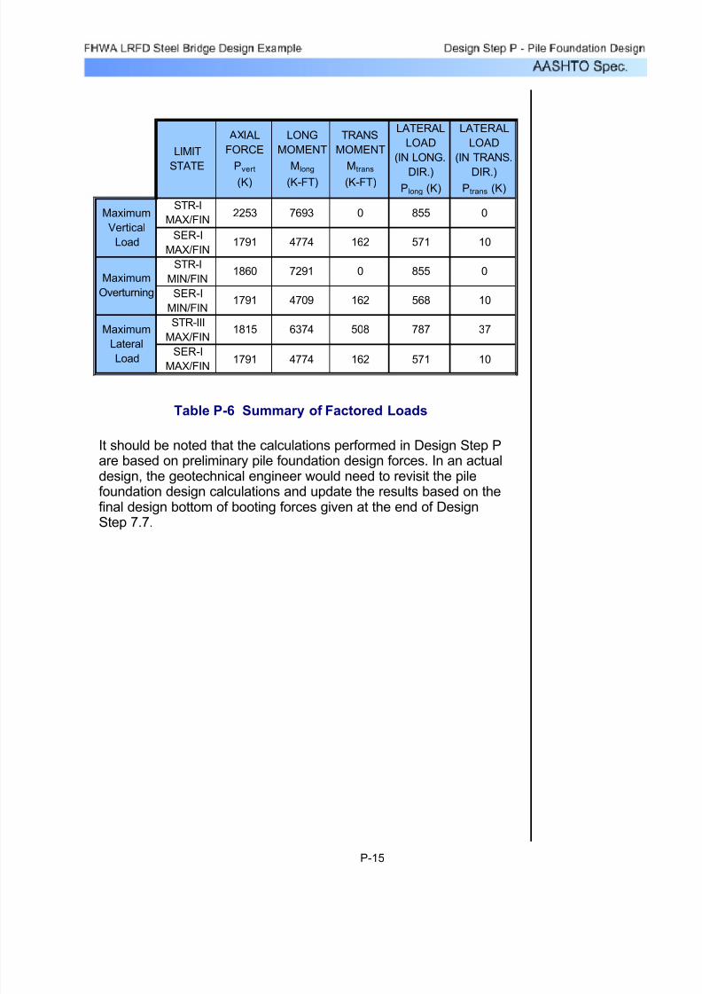
7/29/2019 LRFD steel design.pdf
http://slidepdf.com/reader/full/lrfd-steel-designpdf 546/646
LIMIT
STATE
AXIAL
FORCE
Pvert
(K)
LONG
MOMENT
Mlong
(K-FT)
TRANS
MOMENT
Mtrans
(K-FT)
LATERAL
LOAD
(IN LONG.
DIR.)Plong (K)
LATERAL
LOAD
(IN TRANS.
DIR.)Ptrans (K)
STR-I
MAX/FIN2253 7693 0 855 0
SER-I
MAX/FIN1791 4774 162 571 10
STR-I
MIN/FIN1860 7291 0 855 0
SER-I
MIN/FIN1791 4709 162 568 10
STR-III
MAX/FIN1815 6374 508 787 37
SER-I
MAX/FIN1791 4774 162 571 10
Maximum
Vertical
Load
Maximum
Overturning
Maximum
LateralLoad
Table P-6 Summary of Factored Loads
It should be noted that the calculations performed in Design Step Pare based on preliminary pile foundation design forces. In an actualdesign, the geotechnical engineer would need to revisit the pilefoundation design calculations and update the results based on thefinal design bottom of booting forces given at the end of Design
Step 7.7.
P-15

7/29/2019 LRFD steel design.pdf
http://slidepdf.com/reader/full/lrfd-steel-designpdf 547/646
Bmin 12.736 ft⋅=Preliminary minimum required width
L 46.875 ft⋅=Maximum possible length of footing
The length of the footing is controlled by the length of the abutmentstep required to support the steel beams and the approachroadway. This is determined from previous geometry calculations.
A 597 ft2⋅=The Required area:
Pvert 1791 K⋅=From Design Step P.3,the Maximum service load is
S10.5.2 Presumptive bearing capacity is a service limit state, thuscompare against maximum service load.
SM 3KSF=
STable
10.6.2.3.1-1SM 1.5 TSF⋅=Presumptive bearing capacity
Presumptive Bearing Capacity for loose sand with silt (SM)
Check vertical capacity:
Evaluate a spread footing design:
Design Step P.4 - Verify Need for a Pile Foundation
P-16

7/29/2019 LRFD steel design.pdf
http://slidepdf.com/reader/full/lrfd-steel-designpdf 548/646
In order to resolve the bearing pressure and eccentricity issue, thefooting will have to be widened and the centroid shifted toward thetoe. This can be accomplished by adding width to the toe of thefooting. Note that the issue could also be resolved by adding widthto the heel of the footing, which would increase the weight of soilthat resists overturning. This would require recalculation of theloads and was not pursued here.
Bi
42.563ft=
Bi 10.25 ft⋅=Width of the footing:
S10.6.3.1.5 To prevent excessive loss of contact eB must be less than B/4.
eB 3.92ft=
eB
Mlong
Pvert
=
Pvert 1860 K⋅=
Mlong 7291 K⋅ ft⋅=From the loads obtained in Design Step P.3,
eB
Mlong
Pvert
=Mlong
Determine the maximum eccentricity eB in the direction parallel tothe width of the footing (B)
S10.5.3This is a strength limit state thus use strength loads for the case of maximum overturning which is STR I Min.
Excessive loss of contact:
P-17
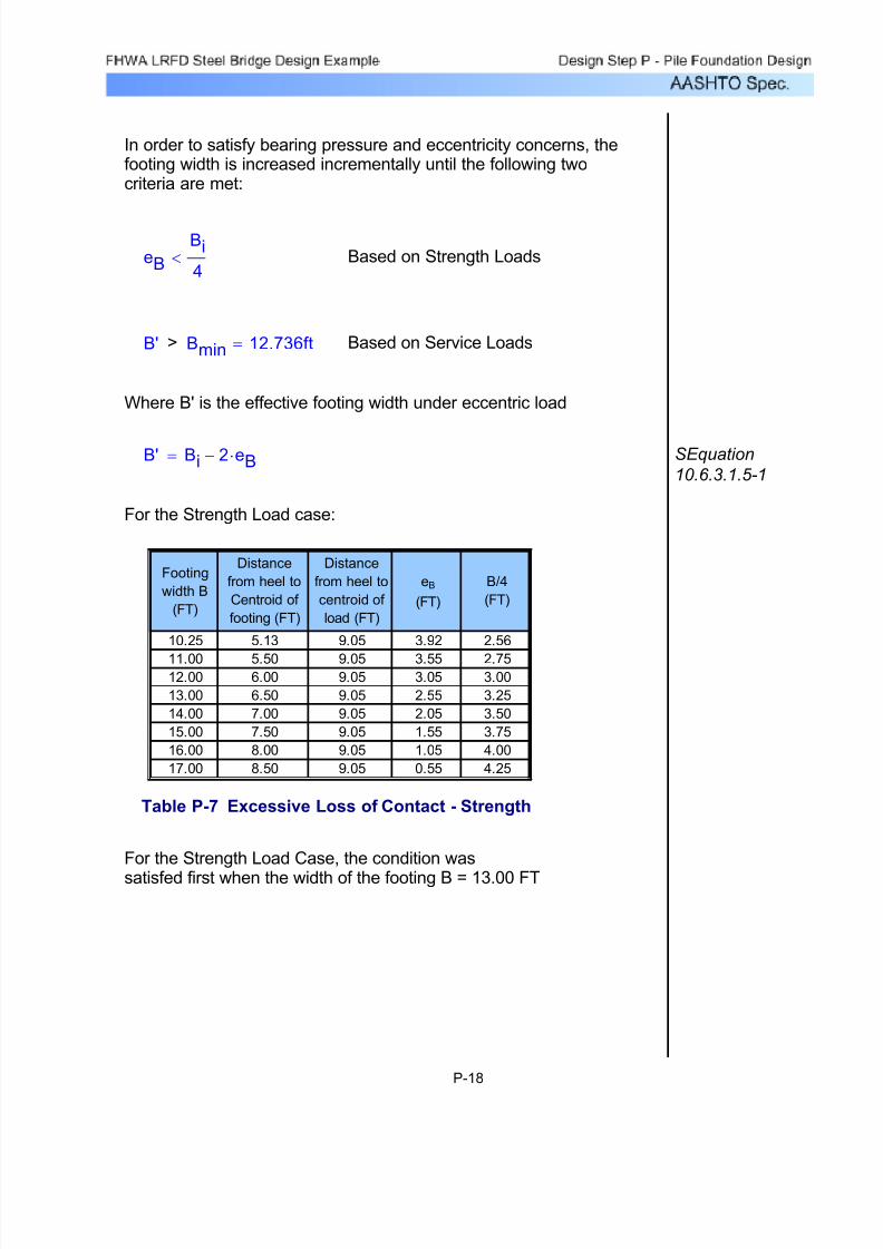
7/29/2019 LRFD steel design.pdf
http://slidepdf.com/reader/full/lrfd-steel-designpdf 549/646
In order to satisfy bearing pressure and eccentricity concerns, thefooting width is increased incrementally until the following twocriteria are met:
eB
Bi
4< Based on Strength Loads
B' > Bmin 12.736ft= Based on Service Loads
Where B' is the effective footing width under eccentric load
B' Bi 2 eB⋅−= SEquation
10.6.3.1.5-1
For the Strength Load case:
Footing
width B
(FT)
Distance
from heel to
Centroid of
footing (FT)
Distance
from heel to
centroid of
load (FT)
eB
(FT)
B/4
(FT)
10.25 5.13 9.05 3.92 2.56
11.00 5.50 9.05 3.55 2.7512.00 6.00 9.05 3.05 3.00
13.00 6.50 9.05 2.55 3.25
14.00 7.00 9.05 2.05 3.50
15.00 7.50 9.05 1.55 3.75
16.00 8.00 9.05 1.05 4.00
17.00 8.50 9.05 0.55 4.25
Table P-7 Excessive Loss of Contact - Strength
For the Strength Load Case, the condition was
satisfed first when the width of the footing B = 13.00 FT
P-18

7/29/2019 LRFD steel design.pdf
http://slidepdf.com/reader/full/lrfd-steel-designpdf 550/646
For the Service Load Case
eB
Mlong
P
vert
=
From the loads obtained from Design Step P.3, Mlong 4774 K⋅ ft⋅=
Pvert 1791 K⋅=
eB
Mlong
Pvert
=
eB 2.67ft=
Footing
width B
(FT)
Distance
from heel to
Centroid of
footing (FT)
Distance
from heel to
centroid of
load (FT)
eB (FT) B' (FT)
10.25 5.13 7.80 2.67 4.91
11.00 5.50 7.80 2.30 6.41
12.00 6.00 7.80 1.80 8.41
13.00 6.50 7.80 1.30 10.41
14.00 7.00 7.80 0.80 12.4115.00 7.50 7.80 0.30 14.41
16.00 8.00 7.80 -0.21 16.41
Table P-8 Presumptive Bearing Pressure - Service
For the Service Load Case, the condition was satisfedfirst when the width of the footing B = 15.00 FT
The first width to satisfy both conditions is 15.00 FT.Which would require the toe of the footing to be extended:
∆B 15 ft⋅ Bi−=
∆B 4.75ft=
This increase may not be possible because it may interfere withroadway drainage, roadside utilities, or the shoulder pavementstructure. However, assume this is not the case and investigatepotential settlement of such a footing.
P-19

7/29/2019 LRFD steel design.pdf
http://slidepdf.com/reader/full/lrfd-steel-designpdf 551/646
L'
B'3.681=atβzShape factor for rigid footing:
ν 0.25=Poisson's ratio of soil, fromDesign Step P.1:
Es 60 TSF⋅=Modulus of elasticity of soil, fromDesign Step P.1:
A 597 ft2= A L' B'⋅=
Therfore, the Effective Area is
B' 12.736 ft=B' Bmin=Width of the footing
L' 46.875 ft=L' L=
Length of footing
A L' B'⋅= L'Effective are of footing:
q0 1.5TSF=
q0 SM= Average bearing pressure on loaded area:
Assume the footing is fully loaded, thus q0 is the presumptivebearing capacity and effective loaded area is as calculatedabove
SEquation
10.6.2.2.3b-1S0
q0 1 ν2
−( )⋅ A0.5⋅
Es βz⋅=
βz
For the granular subsoils, settlement should be esentially elastic thusSettlement (S0) is computed from:
Settlement is a service limit state check.
P-20

7/29/2019 LRFD steel design.pdf
http://slidepdf.com/reader/full/lrfd-steel-designpdf 552/646
The influence value determined above is for a Poisson's ratio of 0.33. A Poisson's ration of 0.25 is used for the soil. Thisdifference is small for the purposes of estimating elastic settlement.
Isb 0.64=I for rigid circular area over stiff base at H/B of 3:
Iinf 0.79=I for rigid circular area over infinite halfspace:
As per NAVFAC DM7.1-212, and DM7.1-213:
Note: This computation assumes an infinite depth of the compressiblelayer. Other computation methods that allow for the rigid base
(NAVFAC DM-7.1-211) indicate the difference between assuming aninfinite compressible layer and a rigid base at a depth equal to 3times the footing width (H/B = 3) below the footing can be estimatedby computing the ratio between appropriate influence factors (I) asfollows:
S0 5.8in=S0 0.49ft=
S0
q0 1 ν2−( )⋅ A0.5⋅
Es βz⋅=
βz 1.18=L'
B'3.681=By interpolation, at
Table P-9 Rigid Footing
STable10.6.2.2.3b-2
L'/B' βz
3 1.155 1.24
From Table 10.6.2.2.3b-2 for rigid footing:
P-21
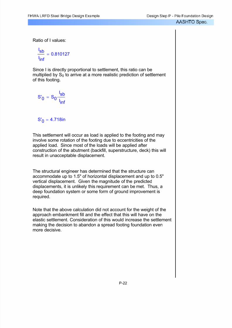
7/29/2019 LRFD steel design.pdf
http://slidepdf.com/reader/full/lrfd-steel-designpdf 553/646
Ratio of I values:
Isb
Iinf
0.810127=
Since I is directly proportional to settlement, this ratio can bemultiplied by S0 to arrive at a more realistic prediction of settlementof this footing.
S'0 S0
Isb
Iinf
⋅=
S'0 4.718in=
This settlement will occur as load is applied to the footing and mayinvolve some rotation of the footing due to eccentricities of theapplied load. Since most of the loads will be applied after construction of the abutment (backfill, superstructure, deck) this willresult in unacceptable displacement.
The structural engineer has determined that the structure canaccommodate up to 1.5" of horizontal displacement and up to 0.5"vertical displacement. Given the magnitude of the predicteddisplacements, it is unlikely this requirement can be met. Thus, adeep foundation system or some form of ground improvement isrequired.
Note that the above calculation did not account for the weight of theapproach embankment fill and the effect that this will have on theelastic settlement. Consideration of this would increase the settlementmaking the decision to abandon a spread footing foundation even
more decisive.
P-22

7/29/2019 LRFD steel design.pdf
http://slidepdf.com/reader/full/lrfd-steel-designpdf 554/646
Design Step P.5 - Select Suitable Pile Type and Size
It will be assumed that for the purposes of this example, groundimprovement methods such as vibro-flotation, vibro replacement,dynamic deep compaction, and others have been ruled out asimpractical or too costly. It is further assumed that drilled shaftfoundations have been shown to be more costly than driven pilefoundations under the existing subsurface conditions (granular, water bearing strata). Thus a driven pile foundation will be designed.
Of the available driven pile types, a steel H-pile end bearing onrock is selected for this application for the following reasons.
1) It is a low displacement pile which will minimize friction in theoverlying soils.
2) It can be driven to high capacities on and into the top weatheredportion of the rock.
3) It is relatively stiff in bending thus lateral deflections will be lessthan for comparably sized concrete or timber piles.
4) Soils have not been shown to be corrosive thus steel loss is notan issue.
P-23
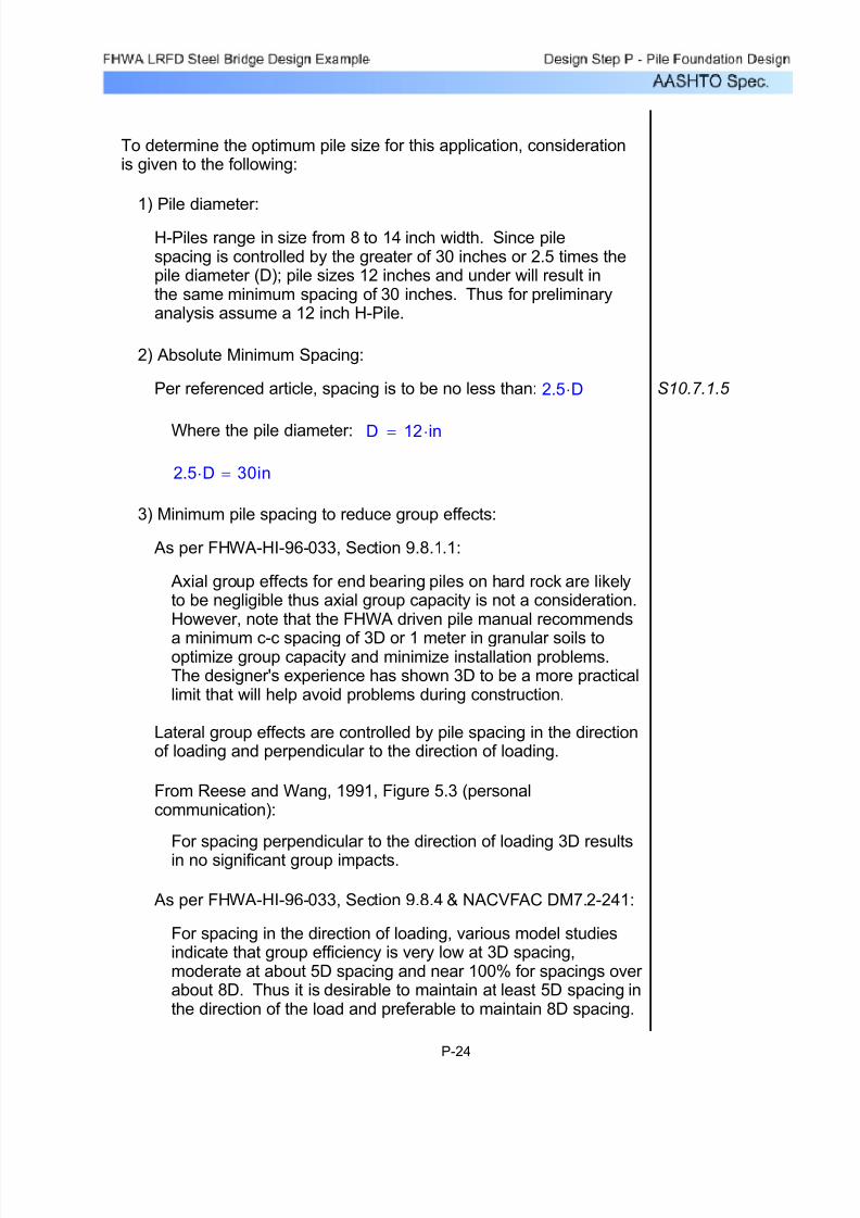
7/29/2019 LRFD steel design.pdf
http://slidepdf.com/reader/full/lrfd-steel-designpdf 555/646
For spacing in the direction of loading, various model studiesindicate that group efficiency is very low at 3D spacing,moderate at about 5D spacing and near 100% for spacings over about 8D. Thus it is desirable to maintain at least 5D spacing inthe direction of the load and preferable to maintain 8D spacing.
As per FHWA-HI-96-033, Section 9.8.4 & NACVFAC DM7.2-241:
For spacing perpendicular to the direction of loading 3D resultsin no significant group impacts.
From Reese and Wang, 1991, Figure 5.3 (personalcommunication):
Lateral group effects are controlled by pile spacing in the directionof loading and perpendicular to the direction of loading.
Axial group effects for end bearing piles on hard rock are likelyto be negligible thus axial group capacity is not a consideration.However, note that the FHWA driven pile manual recommends
a minimum c-c spacing of 3D or 1 meter in granular soils tooptimize group capacity and minimize installation problems.The designer's experience has shown 3D to be a more practicallimit that will help avoid problems during construction.
As per FHWA-HI-96-033, Section 9.8.1.1:
3) Minimum pile spacing to reduce group effects:
2.5 D⋅ 30in=
D 12 in⋅=Where the pile diameter:
S10.7.1.5 2.5 D⋅Per referenced article, spacing is to be no less than:
2) Absolute Minimum Spacing:
H-Piles range in size from 8 to 14 inch width. Since pilespacing is controlled by the greater of 30 inches or 2.5 times thepile diameter (D); pile sizes 12 inches and under will result inthe same minimum spacing of 30 inches. Thus for preliminaryanalysis assume a 12 inch H-Pile.
1) Pile diameter:
To determine the optimum pile size for this application, considerationis given to the following:
P-24
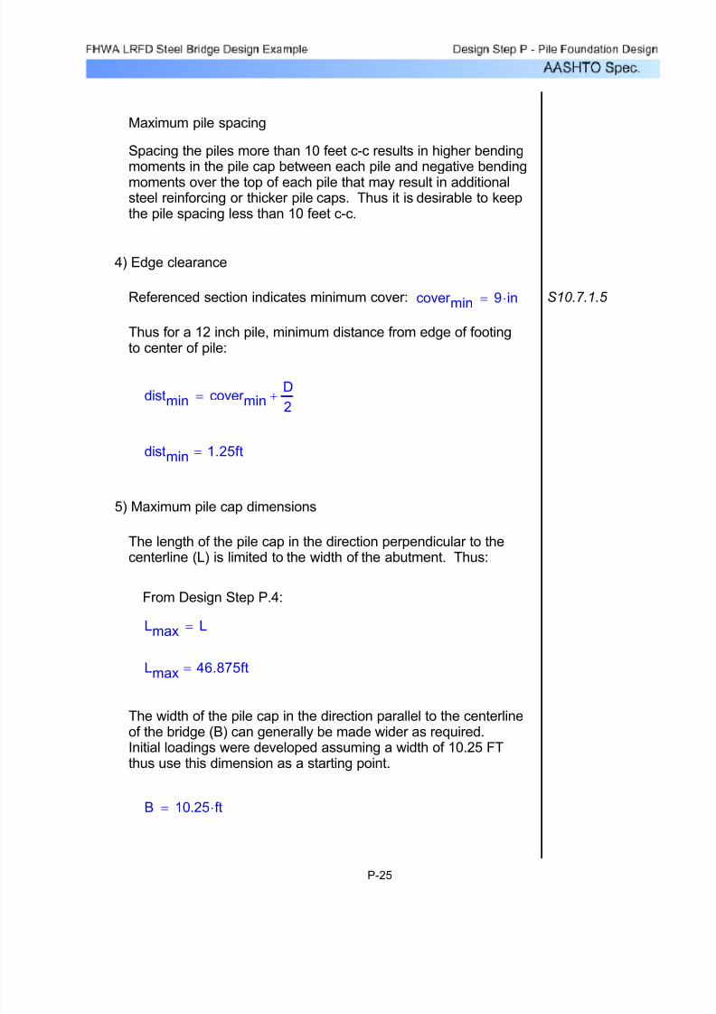
7/29/2019 LRFD steel design.pdf
http://slidepdf.com/reader/full/lrfd-steel-designpdf 556/646
B 10.25 ft⋅=
The width of the pile cap in the direction parallel to the centerlineof the bridge (B) can generally be made wider as required.Initial loadings were developed assuming a width of 10.25 FTthus use this dimension as a starting point.
Lmax 46.875ft=
Lmax L=
From Design Step P.4:
The length of the pile cap in the direction perpendicular to thecenterline (L) is limited to the width of the abutment. Thus:
5) Maximum pile cap dimensions
distmin 1.25ft=
distmin cover minD
2+=
Thus for a 12 inch pile, minimum distance from edge of footing
to center of pile:
S10.7.1.5 cover min 9 in⋅=Referenced section indicates minimum cover:
4) Edge clearance
Spacing the piles more than 10 feet c-c results in higher bendingmoments in the pile cap between each pile and negative bending
moments over the top of each pile that may result in additionalsteel reinforcing or thicker pile caps. Thus it is desirable to keepthe pile spacing less than 10 feet c-c.
Maximum pile spacing
P-25
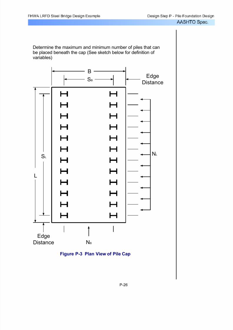
7/29/2019 LRFD steel design.pdf
http://slidepdf.com/reader/full/lrfd-steel-designpdf 557/646
Determine the maximum and minimum number of piles that canbe placed beneath the cap (See sketch below for definition of
variables)
B
SB
NLSL
L
Edge
Distance
Edge
Distance
NB
Figure P-3 Plan View of Pile Cap
P-26
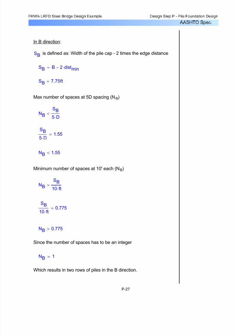
7/29/2019 LRFD steel design.pdf
http://slidepdf.com/reader/full/lrfd-steel-designpdf 558/646
Which results in two rows of piles in the B direction.
NB 1=
Since the number of spaces has to be an integer
NB 0.775>
SB
10 ft⋅0.775=
NB
SB
10 ft⋅>
Minimum number of spaces at 10' each (NB)
NB 1.55<
SB
5 D⋅1.55=
N
B
SB
5 D⋅
<
Max number of spaces at 5D spacing (NB)
SB 7.75ft=
SB B 2 distmin⋅−=
is defined as: Width of the pile cap - 2 times the edge distanceSB
In B direction:
P-27

7/29/2019 LRFD steel design.pdf
http://slidepdf.com/reader/full/lrfd-steel-designpdf 559/646
Which results in 6 to 15 rows of piles in the L direction.
to 14NL 5=
Since the number of spaces has to be an integer
NL 4.438>
SL
10 ft⋅4.438=
NLSL
10 ft⋅>
Minimum number of spaces at 10' each (NL)
NL 14.792<
SL
3 D⋅14.792=
NL
SL
3 D⋅<
Max number of spaces at 3D spacing (NL)
SL 44.375ft=
SL L 2 distmin⋅−=
is defined as: Width of the pile cap - 2 times the edge distanceSL
In L direction:
P-28

7/29/2019 LRFD steel design.pdf
http://slidepdf.com/reader/full/lrfd-steel-designpdf 560/646
RBACK211− K⋅=RFRONT2
1871 K⋅=
Mlong27291 K⋅ ft⋅=Pvert2
1860 K⋅=
For STR I min, from Table P.6:
RBACK1
134 K⋅=RFRONT1
2119 K⋅=
Mlong17963 K⋅ ft⋅=Pvert1
2253 K⋅=
For STR I max, from Table P.6:
ΣMB Mlong−SB
2Pvert⋅− SB RFRONT⋅+= RFRONTΣMB 0=
ΣF
z
P
vert
R
BACK
− R
FRONT
−= R
FRONT
ΣF
z
0=
Summing the forces in the z-direction and the moments about point B:
Figure P-4 Section View of Pile Cap
RFRONTRBACK
Pvert
M long
SB = 7.75'Z
XB F
Using factored loads and diagram below, determine reactions on
the front and back pile rows:
Determine maximum axial load acting on piles
P-29

7/29/2019 LRFD steel design.pdf
http://slidepdf.com/reader/full/lrfd-steel-designpdf 561/646
NOTE: Grade 36 steel is assumed at this stage even though mostH-pile sections are available in higher grades at little or no costdifferential. The need for using a higher strength steel will beinvestigated in future design steps
Fy 36 ksi⋅=
S6.5.4.2 φc 0.6=
NOTE: λ in equation 6.9.4.1-1 is assumed to be zero (because
unbraced length is zero) resulting in the simplified equation shownabove.
Pr φc Fy⋅ As⋅= AsStructural resistance
SEquation
6.9.2.1-1 and
SEquation
6.9.4.1-1
Axial pile resistance is controlled by structural resistance
Assuming the following:
RFRONT15 141.267K=RFRONT6 353.167K=
and
RFRONT15RFRONT
15=RFRONT6
RFRONT6
=
Max anticipated factored pile load can range between:
Since the front row can have 6 - 15 piles,
RFRONT 2119K=
RFRONT max RFRONT
1
RFRONT
2
,( )=
Max axial load on front row of piles:
P-30

7/29/2019 LRFD steel design.pdf
http://slidepdf.com/reader/full/lrfd-steel-designpdf 562/646
Es 29000 ksi⋅=
Zy 32.2 in3⋅=
Note: Plastic section modulus is usedto evaluate nominal moment capacity
Zx 74 in3⋅=
Iyy 127 in4⋅=
Ixx 393 in4⋅=
tw 0.435 in⋅=
tf 0.435 in⋅=
bf 12.045 in⋅=
d 11.78 in⋅=
As 15.5 in2⋅=
Properties of HP 12x53:
For preliminary layout and design, select: HP 12x53
RFRONT15
φc
⎛
⎝
⎞
⎠Fy
6.54in2=and
RFRONT6
φc
⎛
⎝
⎞
⎠Fy
16.35in2=
Compute required pile area to resist the anticipated maximumfactored pile load. The required steel area can range between:
P-31

7/29/2019 LRFD steel design.pdf
http://slidepdf.com/reader/full/lrfd-steel-designpdf 563/646
Design Step P.6 - Determine Nominal Axial Structural Resistance
for Selected Pile Type / Size
Ultimate axial compressive resistance is determined in accordancewith either equation 6.9.4.1-1 or 6.9.4.1-2. The selection of equationis based on the computation of l in equation 6.9.4.1-3 which accountsfor buckling of unbraced sections. Since the pile will be fullyembedded in soil, the unbraced length is zero and therefore l is zero.Based on this this, use equation 6.9.4.1-1 to calculate the nominalcompressive resistance.
S6.9.4.1
Pn 0.66λ
Fy⋅ As⋅= λSEquation
6.9.4.1-1
where:
Fy 36ksi=
As 15.5in2=
λ 0=
Therefore:
Pn 0.66λ
Fy⋅ As⋅=
Pn 558K=
P-32
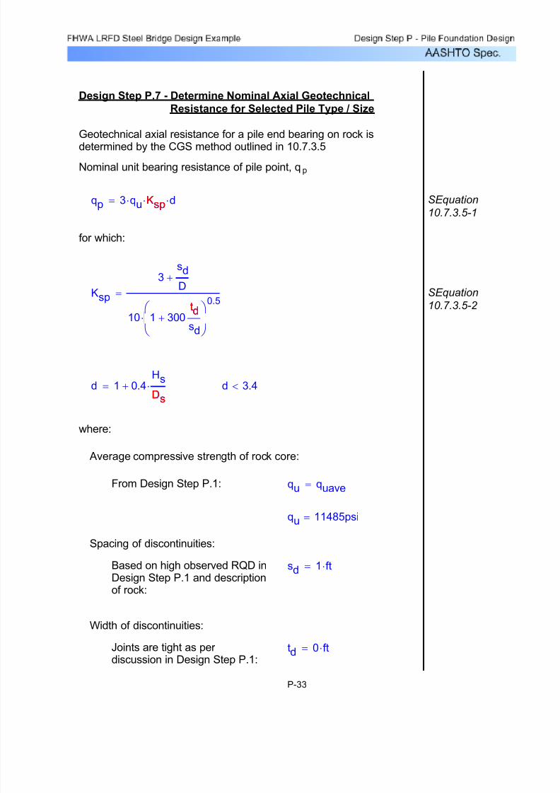
7/29/2019 LRFD steel design.pdf
http://slidepdf.com/reader/full/lrfd-steel-designpdf 564/646
td 0 ft⋅=Joints are tight as per discussion in Design Step P.1:
Width of discontinuities:
sd 1 ft⋅=Based on high observed RQD inDesign Step P.1 and descriptionof rock:
Spacing of discontinuities:
qu 11485psi=
qu quave=From Design Step P.1:
Average compressive strength of rock core:
where:
d 3.4<d 1 0.4Hs
Ds
⋅+=Ds
SEquation
10.7.3.5-2 Ksp
3
sd
D+
10 1 300td
sd
+⎛
⎝
⎞
⎠
0.5
⋅
=td
for which:
SEquation
10.7.3.5-1qp 3 qu⋅ Ksp⋅ d⋅= Ksp
Nominal unit bearing resistance of pile point, qp
Geotechnical axial resistance for a pile end bearing on rock isdetermined by the CGS method outlined in 10.7.3.5
Design Step P.7 - Determine Nominal Axial Geotechnical
Resistance for Selected Pile Type / Size
P-33
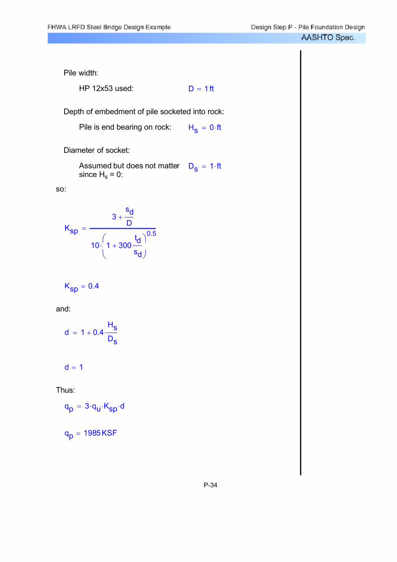
7/29/2019 LRFD steel design.pdf
http://slidepdf.com/reader/full/lrfd-steel-designpdf 565/646
qp 1985 KSF=
qp 3 qu⋅ Ksp⋅ d⋅=Thus:
d 1=
d 1 0.4Hs
Ds
⋅+=
and:
Ksp 0.4=
Ksp
3sd
D+
10 1 300td
sd
+⎛
⎝
⎞
⎠
0.5
⋅
=
so:
Ds 1 ft⋅= Assumed but does not matter since Hs = 0:
Diameter of socket:
Hs 0 ft⋅=Pile is end bearing on rock:
Depth of embedment of pile socketed into rock:
D 1 ft=HP 12x53 used:
Pile width:
P-34
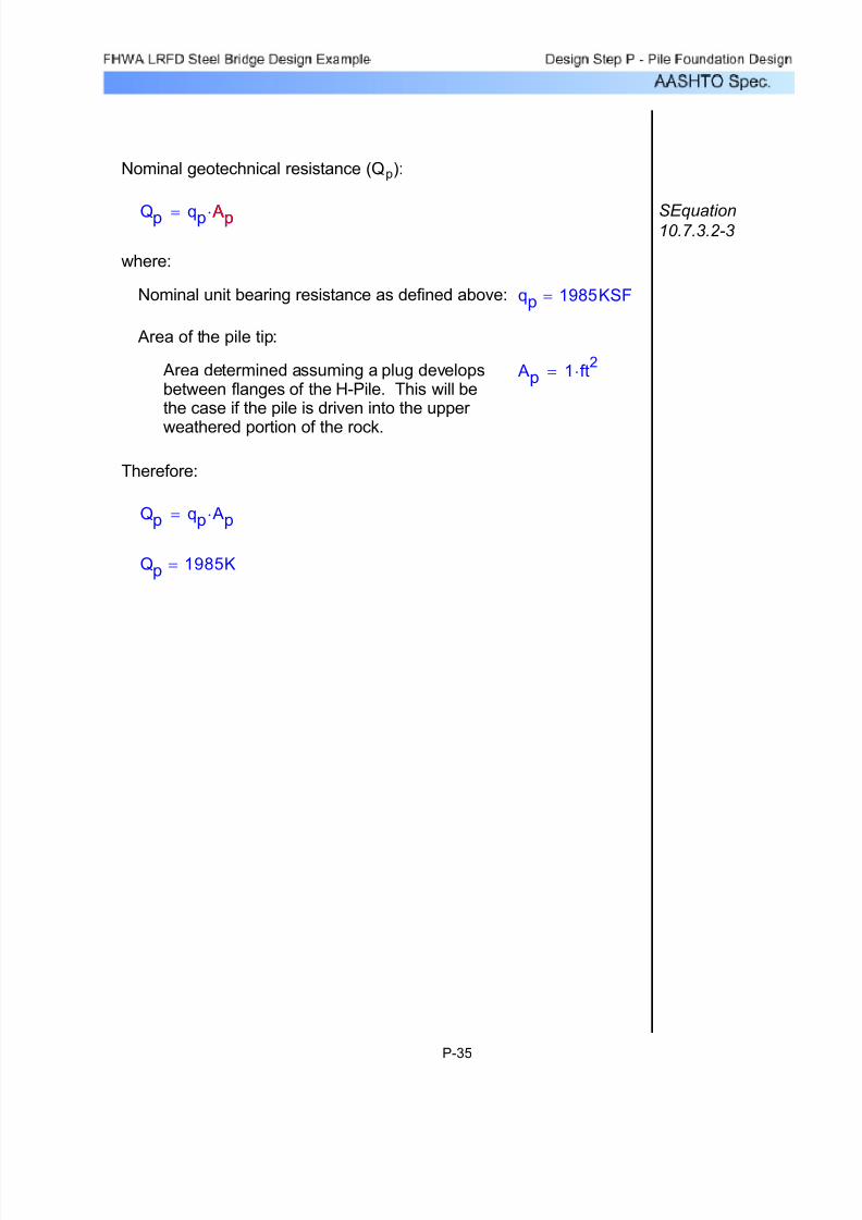
7/29/2019 LRFD steel design.pdf
http://slidepdf.com/reader/full/lrfd-steel-designpdf 566/646
Nominal geotechnical resistance (Qp):
Qp qp Ap⋅= Ap SEquation10.7.3.2-3
where:
Nominal unit bearing resistance as defined above: qp 1985KSF=
Area of the pile tip:
Area determined assuming a plug developsbetween flanges of the H-Pile. This will bethe case if the pile is driven into the upper
weathered portion of the rock.
Ap 1 ft2⋅=
Therefore:
Qp qp Ap⋅=
Qp 1985K=
P-35

7/29/2019 LRFD steel design.pdf
http://slidepdf.com/reader/full/lrfd-steel-designpdf 567/646
Design Step P.8 - Determine Factored Axial Structural
Resistance for Single Pile
Factored Structural Resistance (Pr):
Pr φc Pn⋅= SEquation
6.9.2.1
where:
Resistance factor for H-pile in compression,no damage anticipated:
φc 0.6= S6.5.4.2
Nominal resistance as computed in DesignStep P.6:
Pn 558K=
Therefore:
Pr 334.8K=
P-36
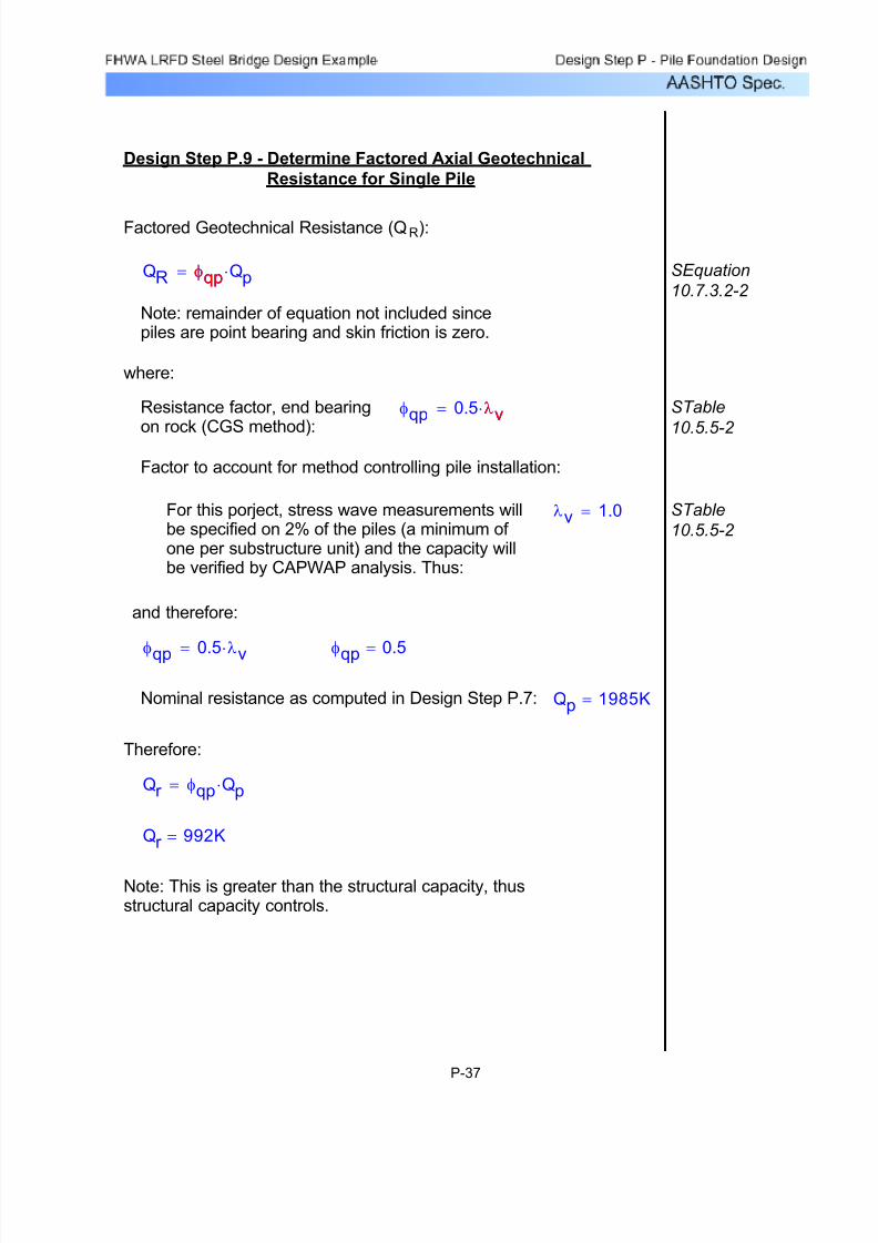
7/29/2019 LRFD steel design.pdf
http://slidepdf.com/reader/full/lrfd-steel-designpdf 568/646
Note: This is greater than the structural capacity, thusstructural capacity controls.
Qr 992K=
Qr φqp Qp⋅=
Therefore:
Qp 1985K=Nominal resistance as computed in Design Step P.7:
φqp 0.5=φqp 0.5 λv⋅=
and therefore:
STable
10.5.5-2 λv 1.0=For this porject, stress wave measurements will
be specified on 2% of the piles (a minimum of one per substructure unit) and the capacity willbe verified by CAPWAP analysis. Thus:
Factor to account for method controlling pile installation:
STable
10.5.5-2
φqp 0.5 λv⋅= λvResistance factor, end bearing
on rock (CGS method):
where:
Note: remainder of equation not included sincepiles are point bearing and skin friction is zero.
SEquation
10.7.3.2-2 QR φqp Qp⋅= φqp
Factored Geotechnical Resistance (QR):
Design Step P.9 - Determine Factored Axial Geotechnical
Resistance for Single Pile
P-37

7/29/2019 LRFD steel design.pdf
http://slidepdf.com/reader/full/lrfd-steel-designpdf 569/646
Design Step P.10 - Check Drivability of Pile
Pile drivability is checked using the computer program WEAP. The
analysis proceeds by selecting a suitable sized hammer. Determiningthe maximum pile stress and driving resistance (BPF) at several levelsof ultimate capacity and plotting a bearing graph relating thesevariables. The bearing graph is then entered at the driving resistanceto be specified for the job (in this case absolute refusal of 20 BPI or 240 BPF will be used) and the ultimate capacity and driving stresscorrelating to that driving resistance is read.
If the ultimate capacity is not sufficient, a bigger hammer is specifiedand the analysis is repeated.
If the driving stress exceeds the permitted driving stress for the pile,a smaller hammer is specified and the analysis is repeated.
Drivability of Piles
If a suitable hammer can not be found that allowsdriving the piile to the required ultimate capacitywithout exceeding the permissible driving stress,modification to the recommended pile type arenecessary. These may include:
Specifying a heavier pile section•Specifying a higher yield stress for the pile steel•Reducing the factored resistance of the pile•
Develop input parameters for WEAP
Driving lengths of piles
The finished pile will likely be 32-33 feet long which includes a 1 footprojection into the pile cap and up to 1' of penetration of the pile tipinto the weathered rock. Therefore assume that 35' long piles will beordered to allow for some variation in subsurface conditions andminimize pile wasted during cut off.
P-38
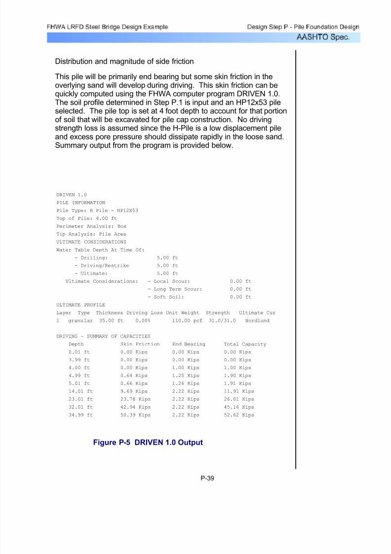
7/29/2019 LRFD steel design.pdf
http://slidepdf.com/reader/full/lrfd-steel-designpdf 570/646
Distribution and magnitude of side friction
This pile will be primarily end bearing but some skin friction in theoverlying sand will develop during driving. This skin friction can be
quickly computed using the FHWA computer program DRIVEN 1.0.The soil profile determined in Step P.1 is input and an HP12x53 pileselected. The pile top is set at 4 foot depth to account for that portionof soil that will be excavated for pile cap construction. No drivingstrength loss is assumed since the H-Pile is a low displacement pileand excess pore pressure should dissipate rapidly in the loose sand.Summary output from the program is provided below.
DRIVEN 1.0
PILE INFORMATION
Pile Type: H Pile - HP12X53
Top of Pile: 4.00 ft
Perimeter Analysis: Box
Tip Analysis: Pile Area
ULTIMATE CONSIDERATIONS
Water Table Depth At Time Of:
- Drilling: 5.00 ft
- Driving/Restrike 5.00 ft
- Ultimate: 5.00 ft
Ultimate Considerations: - Local Scour: 0.00 ft
- Long Term Scour: 0.00 ft- Soft Soil: 0.00 ft
ULTIMATE PROFILE
Layer Type Thickness Driving Loss Unit Weight Strength Ultimate Cur
1 granular 35.00 ft 0.00% 110.00 pcf 31.0/31.0 Nordlund
DRIVING – SUMMARY OF CAPACITIES
Depth Skin Friction End Bearing Total Capacity
0.01 ft 0.00 Kips 0.00 Kips 0.00 Kips
3.99 ft 0.00 Kips 0.00 Kips 0.00 Kips
4.00 ft 0.00 Kips 1.00 Kips 1.00 Kips
4.99 ft 0.64 Kips 1.25 Kips 1.90 Kips
5.01 ft 0.66 Kips 1.26 Kips 1.91 Kips
14.01 ft 9.69 Kips 2.22 Kips 11.91 Kips
23.01 ft 23.78 Kips 2.22 Kips 26.01 Kips
32.01 ft 42.94 Kips 2.22 Kips 45.16 Kips
34.99 ft 50.39 Kips 2.22 Kips 52.62 Kips
Figure P-5 DRIVEN 1.0 Output
P-39

7/29/2019 LRFD steel design.pdf
http://slidepdf.com/reader/full/lrfd-steel-designpdf 571/646
Figure P-6 Bearing Capacity
From this analysis, the side friction during driving will vary in atriangular distribution, and will be about:
Qs 50 K⋅=
The distribution will start 4 feet below the top of the pile which is:
4 ft⋅35 ft⋅
11%= below the top of the pile.
The desired factored resistance was determined in Design Step P.8and is controlled by structural resistance of the pile. This value is:
Pr 334.8K=
The ultimate resistance that must be achieved during wave equationanalysis will be this value divided by the appropriate resistance factor for wave equation analysis + the estimated side friction.
NOTE: Side friction is added here because downdrag is expectedto reduce or reverse the skin friction in the final condition.Therefore, sufficient point capacity must be developed duringdriving to adequately resist all applied loads plus the downdrag.
P-40

7/29/2019 LRFD steel design.pdf
http://slidepdf.com/reader/full/lrfd-steel-designpdf 572/646
φ 0.65 λv⋅= STable
10.5.5-2 From Design Step P.9:
λv 1=
Thus:
φ 0.65=
and
QP
Pr
φ=
QP 515K=
At this Ultimate point resistance the percent side friction is:
Qs
Qs QP+9%=
and the resistance required by wave equation analysis is:
Qreq Qs QP+=
Qreq 565K=
P-41

7/29/2019 LRFD steel design.pdf
http://slidepdf.com/reader/full/lrfd-steel-designpdf 573/646
Use toe damping and toe quake for pile toe.
TQ 0.05 in⋅=Toe Quake:
DIMTD 0.05=Toe Damping:
SQ 0.1 in⋅=Skin Quake:
DIMSD 0.05=Skin Damping:
Hard Sandstone
Use skin damping and skin quake for pile shaft.
TQ 0.1 in⋅=Toe Quake:
DIMTD 0.15=Toe Damping:
SQ 0.1 in⋅=Skin Quake:
DIMSD 0.2=Skin Damping:
Loose Sand
The parameters for loose sand and hard sandstone wereestimated based on local experience with similar soils.
Damping Factors
Case damping factors are used here because of experience with similar jobs. In general, Smithdamping factors are preferred. In this case, the Smithdamping factors would likely give very similar results towhat is computed using the selected Case dampingfactors.
Soil parameters (use Case damping factors):
P-42
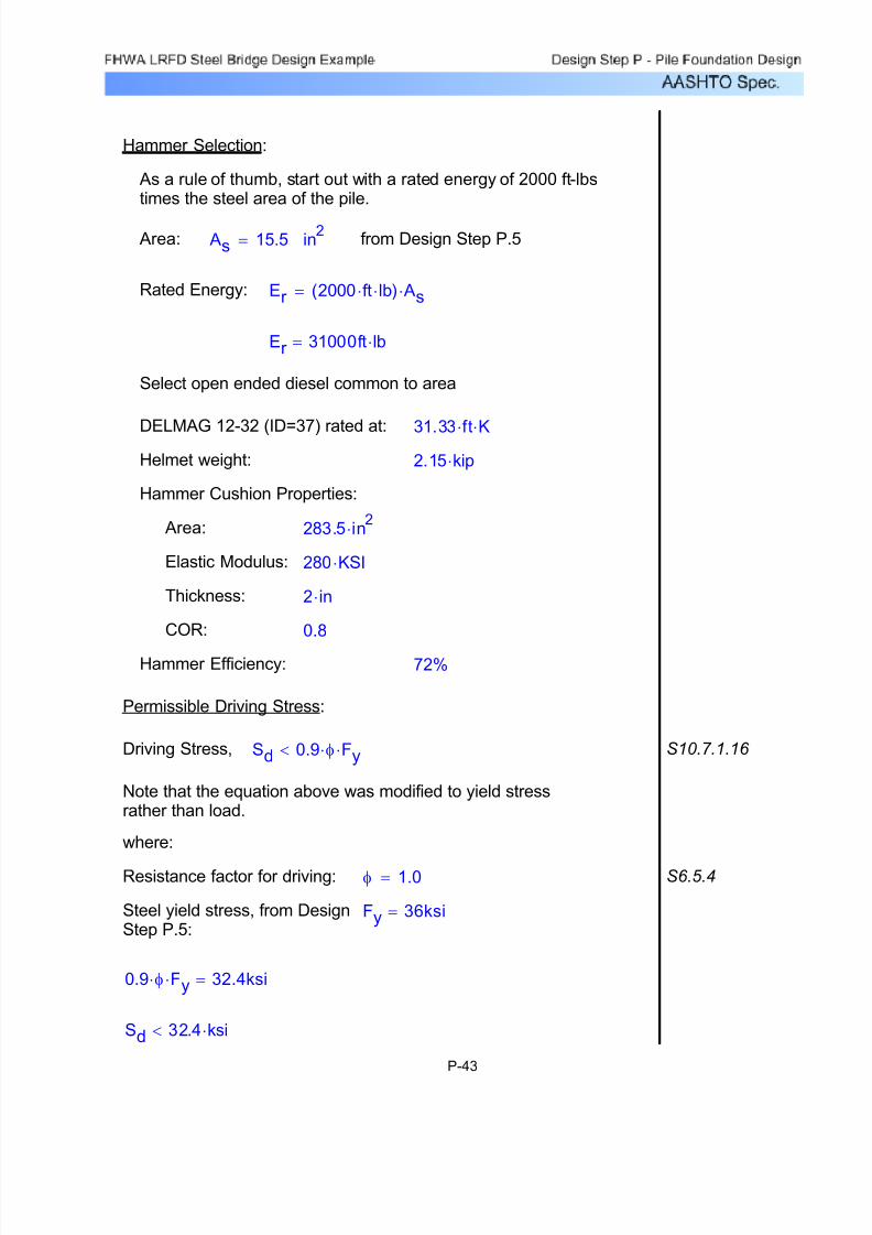
7/29/2019 LRFD steel design.pdf
http://slidepdf.com/reader/full/lrfd-steel-designpdf 574/646
Thickness: 2 in⋅
COR: 0.8
Hammer Efficiency: 72%
Permissible Driving Stress:
Driving Stress, Sd 0.9 φ⋅ Fy⋅< S10.7.1.16
Note that the equation above was modified to yield stressrather than load.
where:
Resistance factor for driving: φ 1.0= S6.5.4
Steel yield stress, from DesignStep P.5:
Fy 36ksi=
0.9 φ⋅ Fy⋅ 32.4ksi=
Sd 32.4 ksi⋅<
Hammer Selection:
As a rule of thumb, start out with a rated energy of 2000 ft-lbstimes the steel area of the pile.
Area: As 15.5= in2
from Design Step P.5
Rated Energy: Er 2000 ft⋅ lb⋅( ) As⋅=
Er 31000ft lb⋅=
Select open ended diesel common to area
DELMAG 12-32 (ID=37) rated at: 31.33 ft⋅ K⋅Helmet weight: 2.15 kip⋅
Hammer Cushion Properties:
Area: 283.5 in2⋅
Elastic Modulus: 280 KSI⋅
P-43
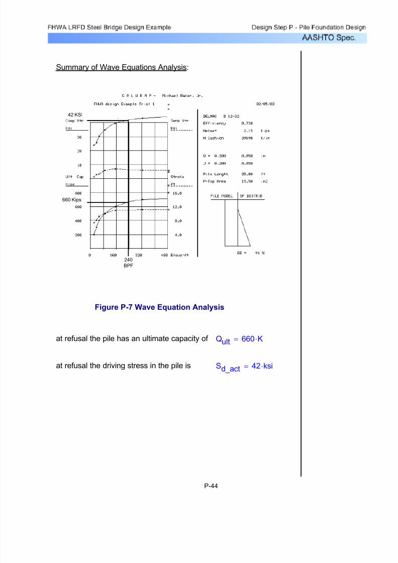
7/29/2019 LRFD steel design.pdf
http://slidepdf.com/reader/full/lrfd-steel-designpdf 575/646
Summary of Wave Equations Analysis:
42 KSI
660 Kips
240
BPF
Figure P-7 Wave Equation Analysis
at refusal the pile has an ultimate capacity of Qult 660 K⋅=
at refusal the driving stress in the pile is Sd_act 42 ksi⋅=
P-44

7/29/2019 LRFD steel design.pdf
http://slidepdf.com/reader/full/lrfd-steel-designpdf 576/646
Hammer Cushion Properties same as before
23.59 ft⋅ kip⋅DELMAG D 12 (ID=3) rated at
Try reducing hammer energy
This condition is not satisfied - no good.
Sd_act 42ksi=>Sd 32.4 ksi⋅=
SD Sd_act>
The permissible driving stress exceeds the actual value
OKQreq 565K=>Qult 660K=
Qult Qreq>
The ultimate capacity exceeds that required
Check:
P-45
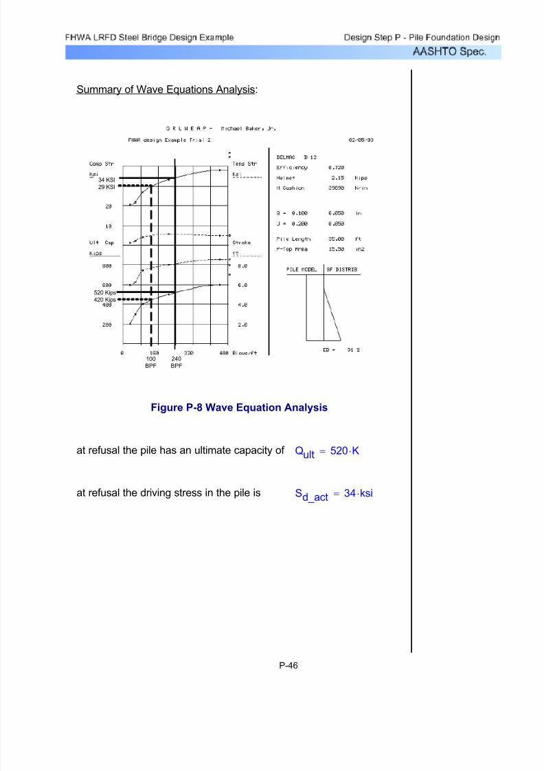
7/29/2019 LRFD steel design.pdf
http://slidepdf.com/reader/full/lrfd-steel-designpdf 577/646
Summary of Wave Equations Analysis:
34 KSI
29 KSI
520 Kips
420 Kips
100
BPF
240
BPF
Figure P-8 Wave Equation Analysis
at refusal the pile has an ultimate capacity of Qult 520 K⋅=
at refusal the driving stress in the pile is Sd_act 34 ksi⋅=
P-46

7/29/2019 LRFD steel design.pdf
http://slidepdf.com/reader/full/lrfd-steel-designpdf 578/646
Based on above analysis, no hammer can possibly drive this pileto the required capacity without exceeding the permissibledriving stress.
Is pile drivable to minimum of Ultimate Geotechnical Axial
Resistance or Ultimate Structural Resistance without piledamage?
A decision must be made at this point:
This condition is not satisfied - no good.
Sd_act 34ksi=>Sd 32.4 ksi⋅=
S
D
S
d_act
>
The permissible driving stress exceeds the actual value
This condition is not satisfied - no good
Qreq 565K=>Qult 520K=
Qult Qreq>
The ultimate capacity exceeds that required
Check:
P-47

7/29/2019 LRFD steel design.pdf
http://slidepdf.com/reader/full/lrfd-steel-designpdf 579/646
There are 2 approaches to resolving this problem
1) Reduce the factored resistance of the pile to a value thatcan be achieved without over stressing the pile.
Based on the above bearing graph and allowing for sometolerance in the driving stress (requiring the contractor toselect a driving system that produces exactly 32.4 KSI inthe pile is unreasonable) a reasonable driven capacity isestimated. Using a minimum driving stress of 29 KSI (0.8Fy) the penetration resistance is about 100 BPF and theultimate capacity would be:
Qult 420 K⋅=
This value includes skin friction during driving which wasset in the program to be 9% of the ultimate resistance.Therefore, point resistance at this driving stress would be:
Qp 91% Qult⋅= Qp 382.2K=
and:
φ 0.65=
QR φ Qp⋅= QR 248.43K=
P-48
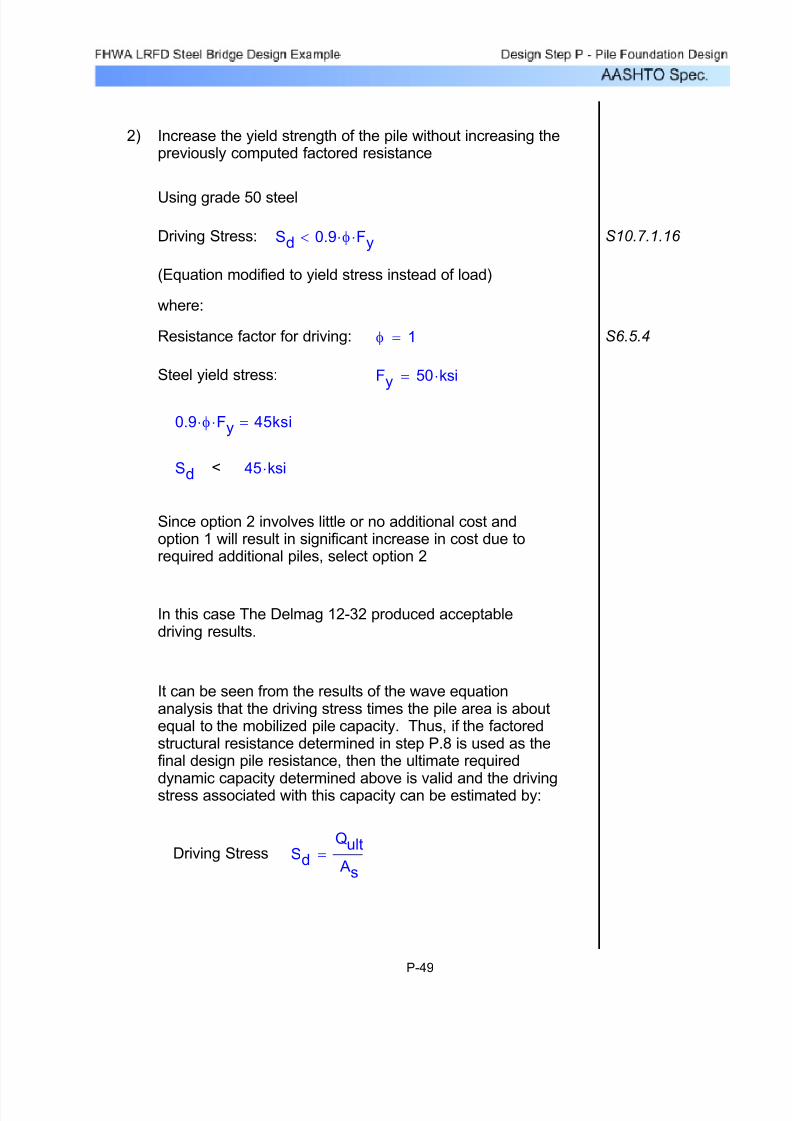
7/29/2019 LRFD steel design.pdf
http://slidepdf.com/reader/full/lrfd-steel-designpdf 580/646
Sd
Qult
As
=Driving Stress
It can be seen from the results of the wave equationanalysis that the driving stress times the pile area is aboutequal to the mobilized pile capacity. Thus, if the factoredstructural resistance determined in step P.8 is used as thefinal design pile resistance, then the ultimate required
dynamic capacity determined above is valid and the drivingstress associated with this capacity can be estimated by:
In this case The Delmag 12-32 produced acceptabledriving results.
Since option 2 involves little or no additional cost andoption 1 will result in significant increase in cost due torequired additional piles, select option 2
45 ksi⋅<Sd
0.9 φ⋅ Fy⋅ 45ksi=
Fy 50 ksi⋅=Steel yield stress:
S6.5.4φ 1=Resistance factor for driving:
where:
(Equation modified to yield stress instead of load)
S10.7.1.16 Sd 0.9 φ⋅ Fy⋅<Driving Stress:
Using grade 50 steel
Increase the yield strength of the pile without increasing thepreviously computed factored resistance
2)
P-49

7/29/2019 LRFD steel design.pdf
http://slidepdf.com/reader/full/lrfd-steel-designpdf 581/646
Qp 523.5K=
As defined previouslyQs 50K=
Qp Qult Qs−=
Qult 573.5K=
Qult Sd_min As⋅=
Sd_min 37 ksi⋅=Using a minimum driving stress of
Thus, so long as the contractor selects a hammer that willproduce a driving stress between about 37 and 45 KSI atrefusal, an acceptable driven capacity should be achievedduring construction.
Sd 36.5ksi=
Sd
Qult
As
=Driving Stress
As 15.5 in2⋅=Pile area, from Design Step 9.5:
Qult 565 K⋅=Ultimate required capacity aspreviously determined bywave equation analysis:
where:
P-50

7/29/2019 LRFD steel design.pdf
http://slidepdf.com/reader/full/lrfd-steel-designpdf 582/646
Pn 775K=
λ 0=
As 15.5in2=
Fy 50ksi=
PnNominal compressive resistance:
where
SEquation
6.9.4.1-1Pn 0.66
λFy⋅ As⋅=
Recompute structural resistance based on higher yield steel,
as in Design Step P.6
QR 340.275K=
QR φ Qp⋅=
Q
p
523.5K=
φ 0.65=
QR φ Qp⋅=
and the minimum driven resistance is
Again, side friction is subtracted from the ultimate capacitysince it will be present during driving but will not be presentin the final condition. Resistance is based on the pointresistance achieved during driving the pile to refusal.
P-51
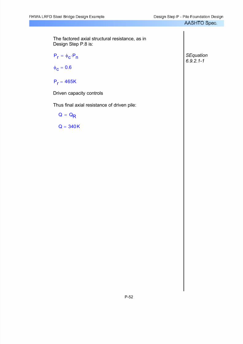
7/29/2019 LRFD steel design.pdf
http://slidepdf.com/reader/full/lrfd-steel-designpdf 583/646
The factored axial structural resistance, as inDesign Step P.8 is:
Pr φc Pn⋅= SEquation
6.9.2.1-1φc 0.6=
Pr 465K=
Driven capacity controls
Thus final axial resistance of driven pile:
Q QR=
Q 340K=
P-52

7/29/2019 LRFD steel design.pdf
http://slidepdf.com/reader/full/lrfd-steel-designpdf 584/646
RBACK 134 K⋅=RFRONT 2119K=
From Design Step P.5, the maximum load that needed to be supportedby each row of piles was calculated.
Additional piles will be required to resist the over turning moment.
PilesN 6.6=
NPvert
Pf
=
Pf QR=
QR 340K=The final controlling factored resistance for the
selected pile type, from Design Step P.10:
Pvert 2253 K⋅=The maximum factored vertical load on theabutment, from Design Step P.3, Load CaseSTR I max:
where:
NP
vertQR
=
The minimum number of piles to support the maximum factored verticalload is:
The purpose of this step is to produce a suitable pile layout beneaththe pile cap that results in predicted factored axial loads in any of thepiles that are less than the final factored resistance for the selectedpiles. A brief evaluation of lateral resistance is also included butlateral resistance is more fully investigated in step P.13
Design Step P.11 - Do Preliminary Pile Layout Based on Factored
Loads and Overturning Moments
P-53

7/29/2019 LRFD steel design.pdf
http://slidepdf.com/reader/full/lrfd-steel-designpdf 585/646
This is approaching the maximum pile spacing identified in Step 5 thusset the back row of piles to the same spacing. This will result in theback row of piles being under utilized for axial loads. However, theadditional piles are expected to be necessary to help handle lateralloads and to resist downdrag loads that will be applied to the back rowonly. Further, a load case in which the longitudinal loads such astemperature and braking loads are reversed will increase the loads onthe back row.
Set c-c spacing of piles = 7' 4"
s 7.396ft=
sSL
NFRONT 1−=c-c spacing of piles:
SL 44.375ft=The length of footing availablefor piles, from Design Step P.5:
where:
sSL
NFRONT
=c-c spacing of piles:
This results in a pile spacing of:
PilesNFRONT 7=
Additional load in the corner pile will come from the lateral momentbut this is small, so start with 7 piles in the front row.
PilesNFRONT 6.2=
NFRONT
RFRONT
Pf
=
The required number of piles in the front row is determined as above.
P-54
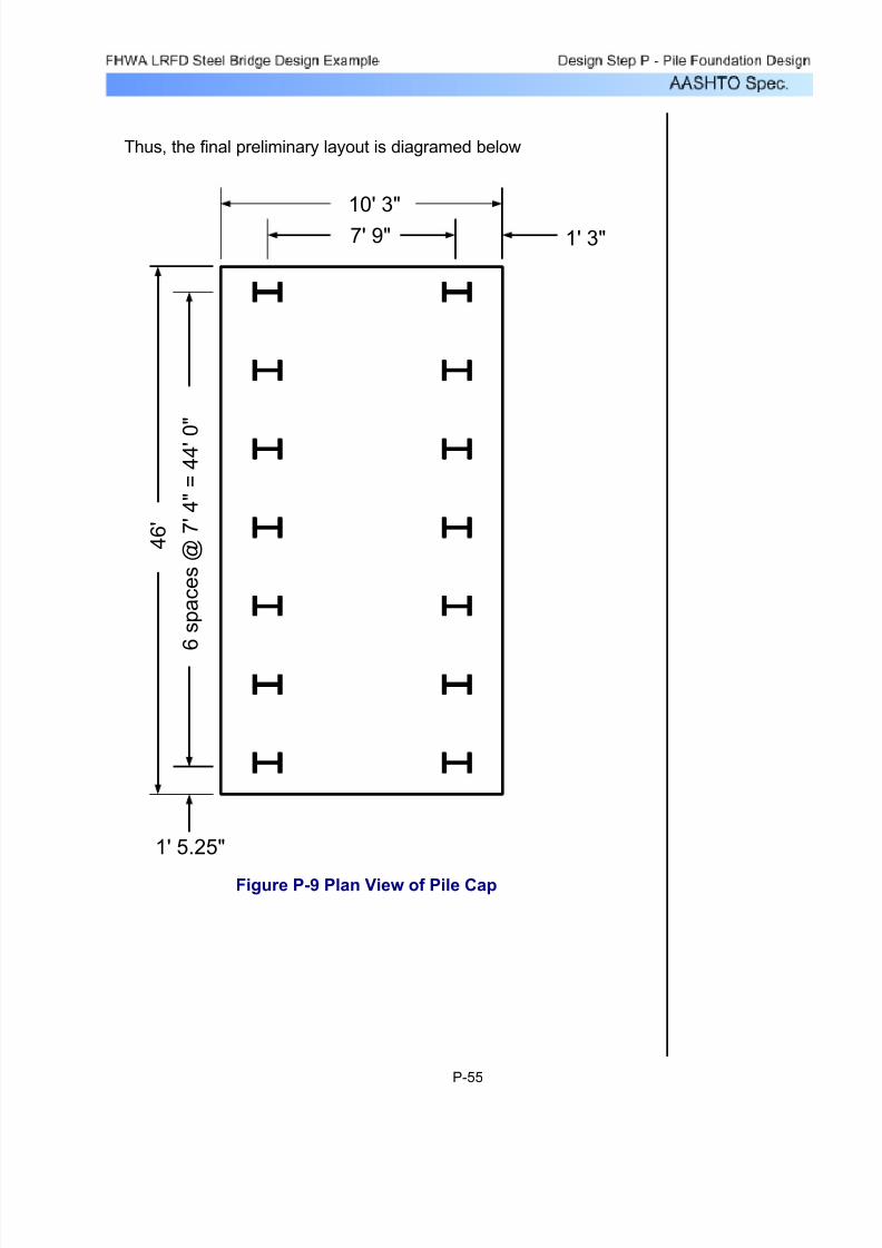
7/29/2019 LRFD steel design.pdf
http://slidepdf.com/reader/full/lrfd-steel-designpdf 586/646
Thus, the final preliminary layout is diagramed below
10' 3"
7' 9"
6 s p a c e s @ 7
' 4 " = 4 4 ' 0 "
4 6 '
1' 5.25"
1' 3"
Figure P-9 Plan View of Pile Cap
P-55

7/29/2019 LRFD steel design.pdf
http://slidepdf.com/reader/full/lrfd-steel-designpdf 587/646
Figure P-10 Coordinate System
+z
+x
+y
The coordinate system for the following calculations is providedin Figure P.10:
My 7693 K⋅ ft⋅=
Mx 0 K⋅ ft⋅=
Fz 2253− K⋅=
At x = 0, y = 0
Input Applied Loads:
Calculation of Individual Pile Loads on an Eccentrically Loaded Footing:
Iyy Ixx,Moment of inertia of the pile groupabout the y and x axis respectively:
x' y',Distance from centroid of pile groupto pile in the x and y directions:
F'z M'x, M'y,Vertical load and moments appliedat the centroid of the pile group:
where:
P F'zN
M'xx'Iyy⋅+ M'y
y'Ixx⋅+= y'
The spreadsheet below is used to calculate individual pile loads usingthe following formula:
P-56

7/29/2019 LRFD steel design.pdf
http://slidepdf.com/reader/full/lrfd-steel-designpdf 588/646
Table P-10 is used to calculate the vertical load and moments, and themoment of inertia of the pile group.
Pile
Number x y x' y' x' 2 y' 2 Pile load
1 -3.875 -22 -3.875 -22 15.01563 484 -19.1221
2 3.875 -22 3.875 -22 15.01563 484 -302.735
3 -3.875 -14.6667 -3.875 -14.6667 15.01563 215.111 -19.1221
4 3.875 -14.6667 3.875 -14.6667 15.01563 215.111 -302.735
5 -3.875 -7.33333 -3.875 -7.33333 15.01563 53.7778 -19.1221
6 3.875 -7.33333 3.875 -7.33333 15.01563 53.7778 -302.735
7 -3.875 0 -3.875 0 15.01563 0 -19.1221
8 3.875 0 3.875 0 15.01563 0 -302.735
9 -3.875 7.33333 -3.875 7.333333 15.01563 53.7778 -19.122110 3.875 7.33333 3.875 7.333333 15.01563 53.7778 -302.735
11 -3.875 14.6667 -3.875 14.66667 15.01563 215.111 -19.1221
12 3.875 14.6667 3.875 14.66667 15.01563 215.111 -302.735
13 -3.875 22 -3.875 22 15.01563 484 -19.1221
14 3.875 22 3.875 22 15.01563 484 -302.735
Input Pile Location Calculated Values
Table P-10 Pile Calculations
Sum of the distances in the x direction is zero.
Sum of the distances in the y direction is zero.
Centroids:
yc 0 in⋅=
xc
0 in⋅=
Moment of Inertia about the y axis: Iyy 210.2188 in4⋅=
Moment of Inertia about the x axis: Ixx 3011.556 in2⋅=
P-57

7/29/2019 LRFD steel design.pdf
http://slidepdf.com/reader/full/lrfd-steel-designpdf 589/646
Resolved loads at Centroid:
F'z Fz=
F'z 2253− K=
M'x F'z− yc⋅ Mx+=
M'x 0 K ft⋅=
M'y F'z− xc⋅ My+=
M'y 7693K ft⋅=
Summary of individual pile loads for all load cases:
This table was generated by inserting each load case in thespreadsheet above and recording the resulting pile loads for thatload combination.
Load
Case
STR-I
MAX/FIN
SER-I
MAX/FIN
STR-I
MIN/FIN
SER-I
MIN/FIN
STR-III
MAX/FIN
SER-I
MAX/FIN
Fz = -2253 -1791 -1860 -1791 -1815 -1791
Mx = 0 162 0 162 508 162
My = 7693 4774 7291 4709 6374 4774
1 -19.1 -41.1 1.5 -42.3 -15.9 -41.1
2 -302.7 -217.1 -267.3 -215.9 -250.8 -217.1
3 -19.1 -40.7 1.5 -41.9 -14.6 -40.7
4 -302.7 -216.7 -267.3 -215.5 -249.6 -216.7
5 -19.1 -40.3 1.5 -41.5 -13.4 -40.3
6 -302.7 -216.3 -267.3 -215.1 -248.4 -216.3
7 -19.1 -39.9 1.5 -41.1 -12.1 -39.9
8 -302.7 -215.9 -267.3 -214.7 -247.1 -215.9
9 -19.1 -39.5 1.5 -40.7 -10.9 -39.5
10 -302.7 -215.5 -267.3 -214.3 -245.9 -215.5
11 -19.1 -39.1 1.5 -40.3 -9.7 -39.112 -302.7 -215.1 -267.3 -213.9 -244.7 -215.1
13 -19.1 -38.7 1.5 -39.9 -8.4 -38.7
14 -302.7 -214.7 -267.3 -213.5 -243.4 -214.7
Maximum -302.7 -217.1 -267.3 -215.9 -250.8 -217.1
Minimum -19.1 -38.7 1.5 -39.9 -8.4 -38.7
Pile No.
Table P-11 Individual Loads for All Load Cases
P-58
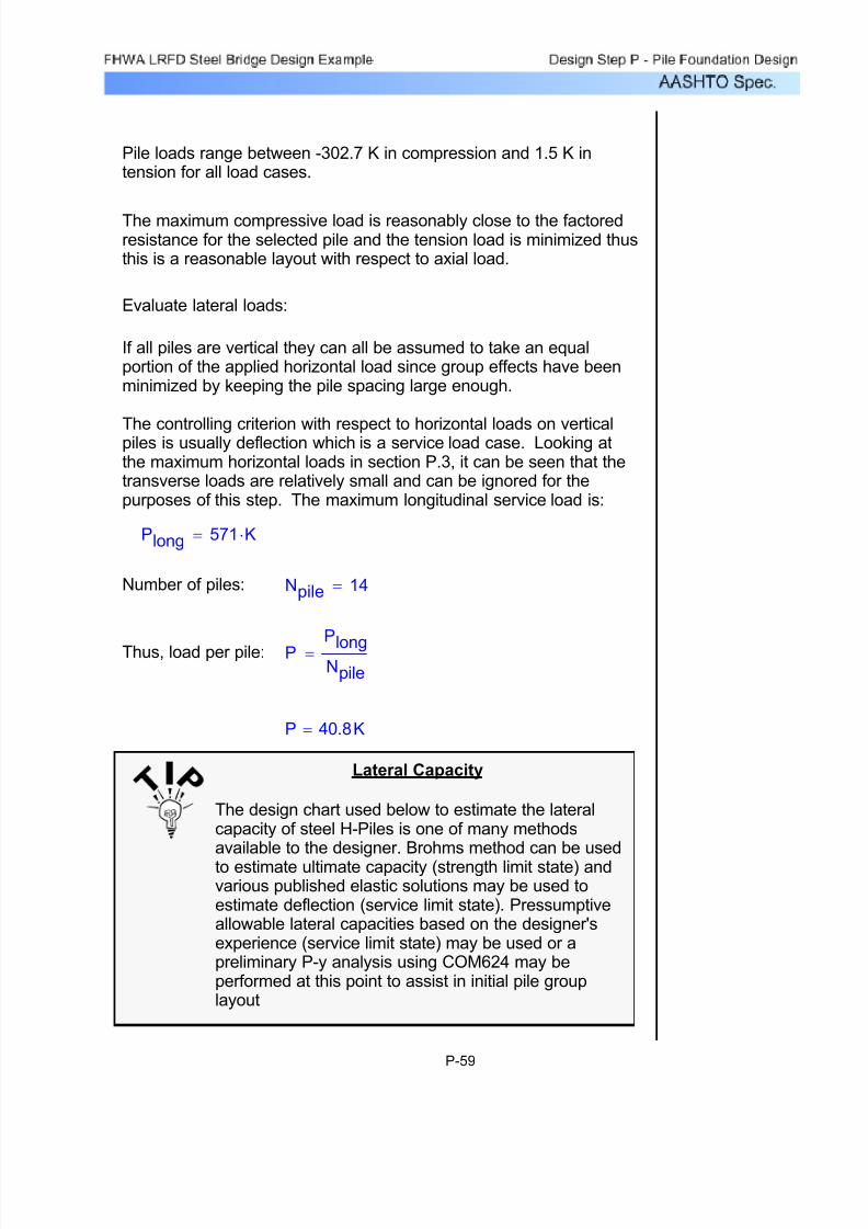
7/29/2019 LRFD steel design.pdf
http://slidepdf.com/reader/full/lrfd-steel-designpdf 590/646
Pile loads range between -302.7 K in compression and 1.5 K intension for all load cases.
The maximum compressive load is reasonably close to the factoredresistance for the selected pile and the tension load is minimized thusthis is a reasonable layout with respect to axial load.
Evaluate lateral loads:
If all piles are vertical they can all be assumed to take an equalportion of the applied horizontal load since group effects have beenminimized by keeping the pile spacing large enough.
The controlling criterion with respect to horizontal loads on verticalpiles is usually deflection which is a service load case. Looking atthe maximum horizontal loads in section P.3, it can be seen that thetransverse loads are relatively small and can be ignored for thepurposes of this step. The maximum longitudinal service load is:
Plong 571 K⋅=
Number of piles: Npile 14=
Thus, load per pile: PP
longNpile
=
P 40.8K=
Lateral Capacity
The design chart used below to estimate the lateralcapacity of steel H-Piles is one of many methodsavailable to the designer. Brohms method can be used
to estimate ultimate capacity (strength limit state) andvarious published elastic solutions may be used toestimate deflection (service limit state). Pressumptiveallowable lateral capacities based on the designer'sexperience (service limit state) may be used or apreliminary P-y analysis using COM624 may beperformed at this point to assist in initial pile grouplayout
P-59

7/29/2019 LRFD steel design.pdf
http://slidepdf.com/reader/full/lrfd-steel-designpdf 591/646
Based on the design chart below, the maximum service load per pilefor an assumed 1.5" deflection (38mm) is:
92KN 20.6K=92KN 20.6K=From PennDOT DM4 Appendix F-20:
92 KN
Figure P-11 Maximum Service Load Per Pile
P-60

7/29/2019 LRFD steel design.pdf
http://slidepdf.com/reader/full/lrfd-steel-designpdf 592/646
Notes on chart:
Solid lines represent load vs deflection for full depthloose saturated sand
I values are moment of inertia for pile about axis
perpendicular to applied load (shown in mm4 x 108)
For HP 12 x 53
Ixx 393 in4⋅=
Ixx 1.636 108× mm
4=
Load in KN is applied at ground surface and pile headis assumed to be 50% fixed
Thus, there probably will not be sufficient lateral load capacity with 14vertical piles. To resolve this, it will be necessary to add more piles or batter some of the piles. Since at least twice as many piles would berequired to handle the anticipated horizontal loads, battering the pilesmakes more sense.
Investigate battering front row of piles at 1:3 (back row of piles notbattered due to lack of vertical load and potential for downdrag)
Total vertical load on front row for each of the load cases is computedby summing the individual pile loads computed above.
P-61
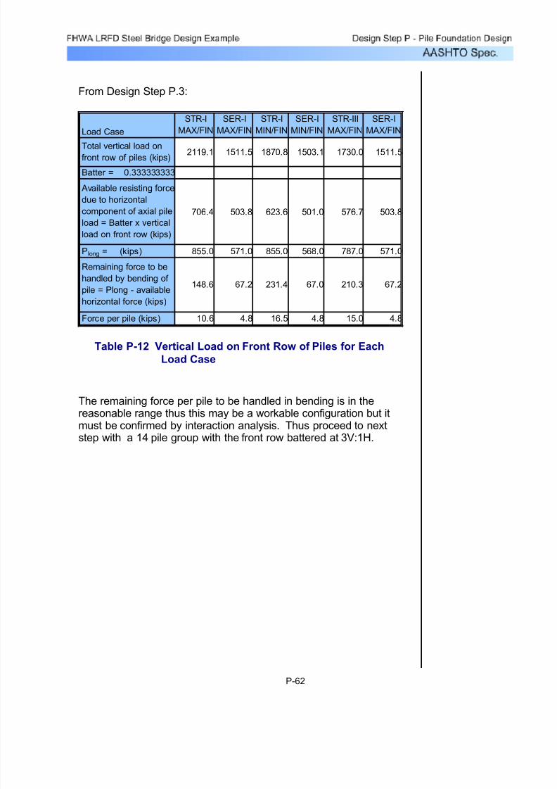
7/29/2019 LRFD steel design.pdf
http://slidepdf.com/reader/full/lrfd-steel-designpdf 593/646
From Design Step P.3:
Load Case
STR-I
MAX/FIN
SER-I
MAX/FIN
STR-I
MIN/FIN
SER-I
MIN/FIN
STR-III
MAX/FIN
SER-I
MAX/FIN
2119.1 1511.5 1870.8 1503.1 1730.0 1511.5
Batter = 0.333333333
706.4 503.8 623.6 501.0 576.7 503.8
Plong = (kips) 855.0 571.0 855.0 568.0 787.0 571.0
148.6 67.2 231.4 67.0 210.3 67.2
Force per pile (kips) 10.6 4.8 16.5 4.8 15.0 4.8
Total vertical load on
front row of piles (kips)
Available resisting force
due to horizontal
component of axial pile
load = Batter x vertical
load on front row (kips)
Remaining force to be
handled by bending of pile = Plong - available
horizontal force (kips)
Table P-12 Vertical Load on Front Row of Piles for Each
Load Case
The remaining force per pile to be handled in bending is in the
reasonable range thus this may be a workable configuration but itmust be confirmed by interaction analysis. Thus proceed to nextstep with a 14 pile group with the front row battered at 3V:1H.
P-62

7/29/2019 LRFD steel design.pdf
http://slidepdf.com/reader/full/lrfd-steel-designpdf 594/646
Design Step P.12 - Evaluate Pile Head Fixity
The performance of the pile group and the resulting pile stresses aregreatly influenced by the degree to which piles are fixed against
rotation at the pile head. This fixity is provided by the pile cap and isa function of the embedment of the pile into the cap, the geometry of the pile group, the stiffness of the pile cap, and the deflection. Eachof these is evaluated below.
S10.7.3.8
Embedment
Research has shown that a pile needs to be embedded 2-3 times itsdiameter into the pile cap in order to develop full fixity. These pileswill be embedded the minimum of 1 foot since the thickness of thepile cap is expected to be only 2.5 feet. Embedding the piles 2 feet
into a 2.5 thick cap places the tops of the piles near the top layer of reinforcing and increases the probability of the pile punching throughthe top of the cap under load. Thus full pile head fixity will likely notdevelop regardless of other factors.
S10.7.1.5
Group geometry
In the transverse direction, there will be 7 rows of piles that whendeflected force the pile cap to remain level. This condition will resultin full fixity of the pile head pending evaluation of other factors. Inthe longitudinal direction there will be only 2 rows of piles whichshould be sufficient to enforce fixity pending evaluation of other factors. However, if the front row of piles is battered and the backrow of piles is left vertical, the pile cap will tend to rotate backwardsas it deflects. This could conceivably result in a moment applied tothe pile heads greater than that required to fix the head (i.e. greater than 100% fixity) This backwards rotation of the pile cap isaccounted for in the group analysis so it does not need to beconsidered here.
Pile cap stiffness
Flexing of the pile cap due to applied loads and moments tends toreduce the fixity at the head of the pile. In this case the pile cap isexpected to be relatively thin so this effect becomes important. Thestiffness of the pile cap is accounted for in the group interactionanalysis so this does not effect the evaluation of fixity.
P-63
7/29/2019 LRFD steel design.pdf
http://slidepdf.com/reader/full/lrfd-steel-designpdf 595/646
Deflection
The fixity of a pile is reduced at large deflections due to crackingof the concrete at the bottom of the pile cap. For the vertical pile
group deflections are expected to be large but for the batteredgroup deflections are likely to be small.
Conclusion
Since the group analysis will account for the group geometry andthe stiffness of the pile cap, the remaining factors of embedmentand deflection need to be accounted for. Both of these indicatethat pile head fixity is likely to be somewhere between 25 and75% with the higher values for the battered group. To beconservative, the group will be analyzed with 0 and 100% fixity todetermine the critical conditions for pile stress (usually 100%fixity) and deflection (0 % fixity)
P-64

7/29/2019 LRFD steel design.pdf
http://slidepdf.com/reader/full/lrfd-steel-designpdf 596/646
Each is evaluated below:
Other miscellaneous considerations6)
The torsional response of the soil and rock (T- q)5)
The lateral response of soil (P-y)4)
The axial response of the soil and rock (T-z and Q-z)3)
The location and distribution of applied loads.2)
The location and thickness of the abutment stem. This controls therelative stiffness of the pile cap.
1)
In order to properly use the program, a few additional soil and pilecap properties need to be established. These are:
S10.7.3.11Group interaction analysis will be performed using the computer program FB-Pier developed by FHWA, FloridaDOT and University of
Florida. This program is available from the Bridge Software Instituteassociated with the University of Florida. Version 3 of the program isused in this example.
Design Step P.13 - Perform Pile Soil Interaction Analysis
P-65

7/29/2019 LRFD steel design.pdf
http://slidepdf.com/reader/full/lrfd-steel-designpdf 597/646
Location and thickness of stem.
Previous analysis has developed a preliminary stem thickness of 3.5feet located 2.75' from the toe of the footing. The stem is 15' tall thusthe footing will be thickened to 15' in this zone as shown on the sketchbelow:
10' 3"
7' 9"
6 s p a c
e s @ 7
' 4 " = 4 4 ' 0 "
4 6 '
1' 5.25"
1' 3"
3.5' 2.75'
CL of pile
cap
ZONE OF
THICKENED
FOOTING TO
ACCOUNT FOR
STEM
ASSUMED
LOCATIONS OF
APPLIED LOADS
(typical 3 spots)
Y
X
Figure P-12 Location and Thickness of Stem
P-66

7/29/2019 LRFD steel design.pdf
http://slidepdf.com/reader/full/lrfd-steel-designpdf 598/646
Location of applied loads
The loads as supplied so far were resolved to a point at the center of the footing and the bottom of the pile cap. The loads actually
consist of numerous loads due to earth pressure, superstructure,self weight etc. that are distributed over the proposed structure. Tosimplify the analysis, only the pile cap will be modeled in FB-Pier.The supplied loads will be divided by 3 and applied to the pile capat 3 locations along the length of the stem at the centerline of thepile group. Since the cap will be modeled as a membrane elementat an elevation that corresponds to the base of the pile cap and theloads were supplied at the base of the pile cap, no additionalchanges to the supplied loads and moments are required. Theassumed locations of the applied loads are shown above.
The magnitude of loads and moments are computed from thoseprovided in section P.3 as shown below. The terminology and signconvention has been converted to that used in FB-Pier. Thecoordinate system used is a right handed system as shown in thesketch above with Z pointing down.
Note the loads at each point provided below are in Kip-FT units
LIMIT
STATE
FB-Pier
Load
Case
Fz (K) My (K-FT) Mx (K-FT) Fx (K) Fy (K)
STR-IMAX/FIN
1 751.0 -2564.3 0.0 285.0 0.0
SER-I
MAX/FIN2 597.0 -1591.3 54.0 190.3 3.3
STR-I
MIN/FIN3 620.0 -2430.3 0.0 285.0 0.0
SER-I
MIN/FIN4 597.0 -1569.7 54.0 189.3 3.3
STR-III
MAX/FIN5 605.0 -2124.7 169.3 262.3 12.3
SER-I
MAX/FIN6 597.0 -1591.3 54.0 190.3 3.3
Table P-13 Loads for Each Limit State
P-67
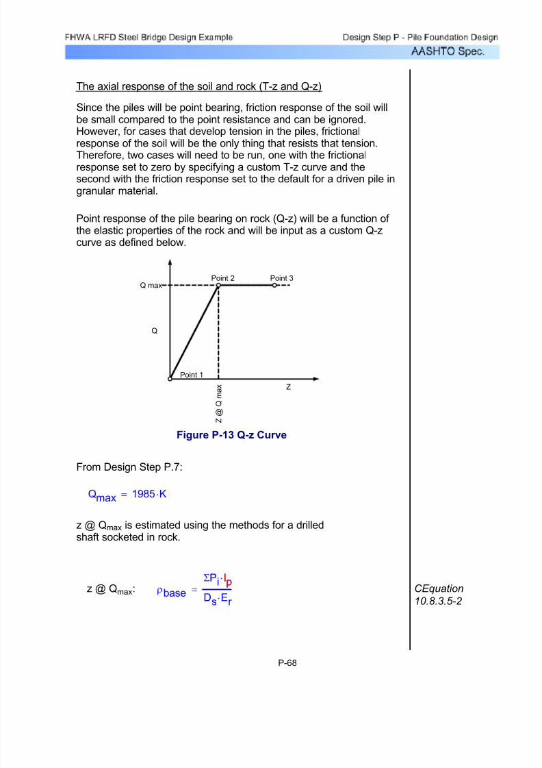
7/29/2019 LRFD steel design.pdf
http://slidepdf.com/reader/full/lrfd-steel-designpdf 599/646
The axial response of the soil and rock (T-z and Q-z)
Since the piles will be point bearing, friction response of the soil willbe small compared to the point resistance and can be ignored.
However, for cases that develop tension in the piles, frictionalresponse of the soil will be the only thing that resists that tension.Therefore, two cases will need to be run, one with the frictionalresponse set to zero by specifying a custom T-z curve and thesecond with the friction response set to the default for a driven pile ingranular material.
Point response of the pile bearing on rock (Q-z) will be a function of the elastic properties of the rock and will be input as a custom Q-zcurve as defined below.
Q maxPoint 2 Point 3
Point 1
Z @ Q
m a x Z
Q
Figure P-13 Q-z Curve
From Design Step P.7:
Qmax 1985 K⋅=
z @ Qmax is estimated using the methods for a drilled
shaft socketed in rock.
z @ Qmax: ρbase
ΣPi Ip⋅
Ds Er ⋅=
IpCEquation
10.8.3.5-2
P-68
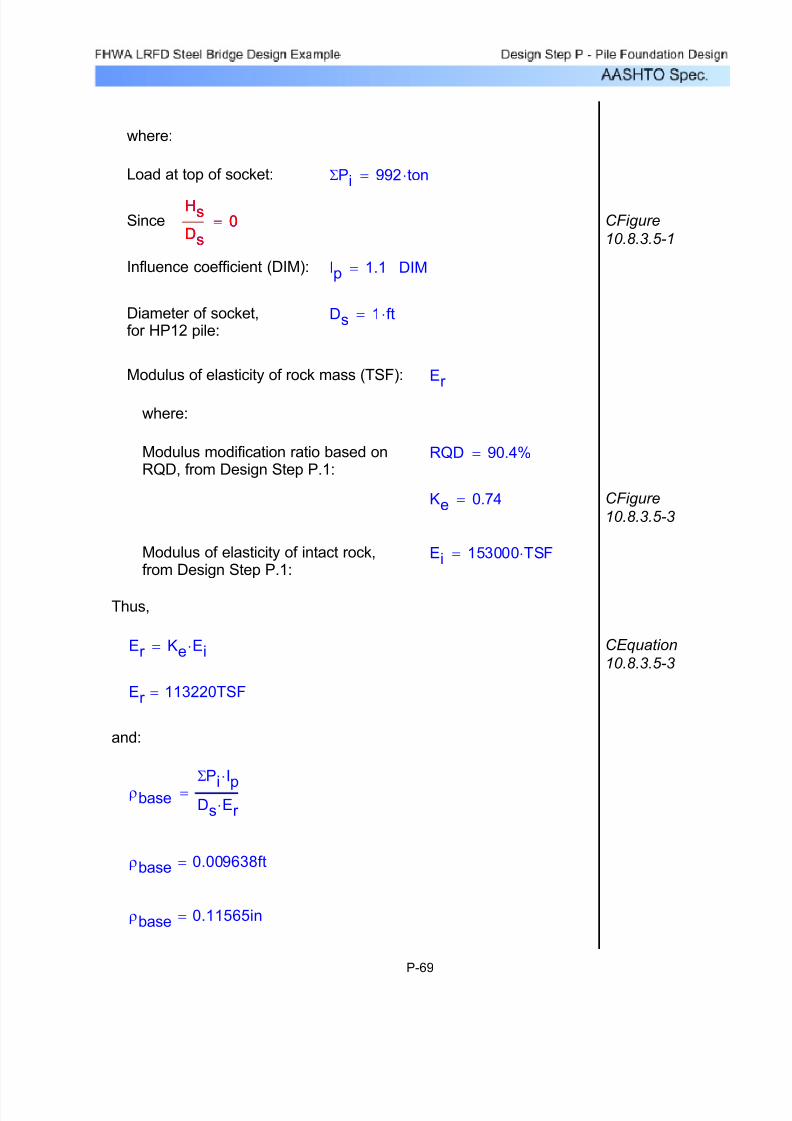
7/29/2019 LRFD steel design.pdf
http://slidepdf.com/reader/full/lrfd-steel-designpdf 600/646
ρbase 0.11565in=
ρbase 0.009638ft=
ρbase
ΣPi
Ip
⋅
Ds Er ⋅=
and:
Er 113220TSF=
CEquation
10.8.3.5-3Er Ke Ei⋅=
Thus,
Ei 153000 TSF⋅=Modulus of elasticity of intact rock,from Design Step P.1:
CFigure
10.8.3.5-3Ke 0.74=
RQD 90.4%=Modulus modification ratio based onRQD, from Design Step P.1:
where:
Er Modulus of elasticity of rock mass (TSF):
Ds 1 ft⋅=Diameter of socket,for HP12 pile:
DIMIp 1.1=Influence coefficient (DIM):
CFigure
10.8.3.5-1
Hs
Ds
0=Hs
Ds
0=Since
ΣPi 992 ton⋅=Load at top of socket:
where:
P-69

7/29/2019 LRFD steel design.pdf
http://slidepdf.com/reader/full/lrfd-steel-designpdf 601/646
Thus Q-z curve is defined by the following points
(refer to the sketch above for location of the points)
Point Q (kips) z (IN)
1 0 0.00
2 1985 0.12
3 1985 2.00
Table P-14 Q-z Curve Points
P-70
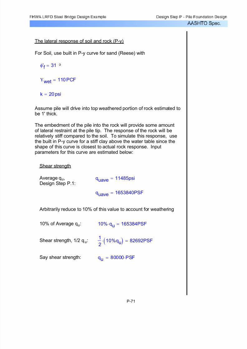
7/29/2019 LRFD steel design.pdf
http://slidepdf.com/reader/full/lrfd-steel-designpdf 602/646
qu 80000 PSF⋅=Say shear strength:
1
2
10%q
u( )⋅ 82692PSF=Shear strength, 1/2 qu:
10% qu⋅ 165384PSF=10% of Average qu:
Arbitrarily reduce to 10% of this value to account for weathering
quave 1653840PSF=
quave 11485psi= Average qu,
Design Step P.1:
Shear strength
The embedment of the pile into the rock will provide some amountof lateral restraint at the pile tip. The response of the rock will berelatively stiff compared to the soil. To simulate this response, usethe built in P-y curve for a stiff clay above the water table since theshape of this curve is closest to actual rock response. Inputparameters for this curve are estimated below:
Assume pile will drive into top weathered portion of rock estimated tobe 1' thick.
k 20psi=
Υwet 110PCF=
oφ'f 31=
For Soil, use built in P-y curve for sand (Reese) with
The lateral response of soil and rock (P-y)
P-71
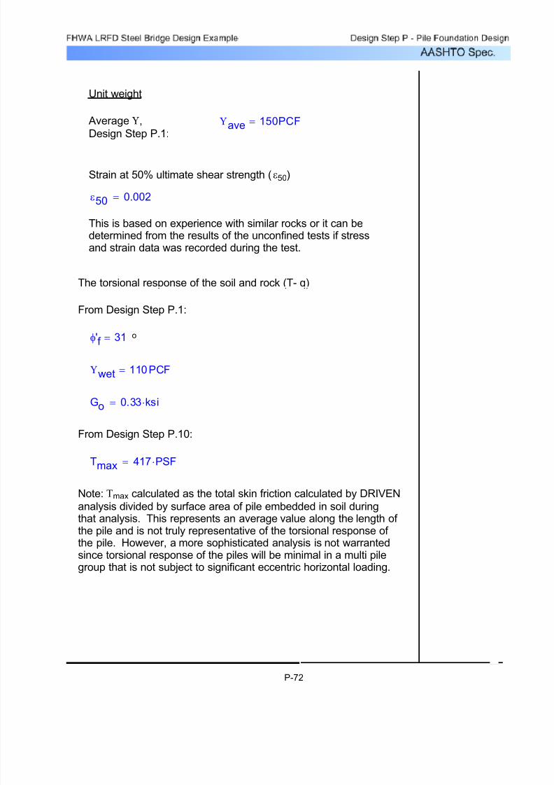
7/29/2019 LRFD steel design.pdf
http://slidepdf.com/reader/full/lrfd-steel-designpdf 603/646
Unit weight
Average Υ,
Design Step P.1:
Υave 150PCF=
Strain at 50% ultimate shear strength (ε50)
ε50 0.002=
This is based on experience with similar rocks or it can bedetermined from the results of the unconfined tests if stressand strain data was recorded during the test.
The torsional response of the soil and rock (T- q)
From Design Step P.1:
φ'f 31= o
Υwet 110PCF=
Go 0.33 ksi⋅=
From Design Step P.10:
Tmax 417 PSF⋅=
Note: Τmax calculated as the total skin friction calculated by DRIVEN
analysis divided by surface area of pile embedded in soil duringthat analysis. This represents an average value along the length of the pile and is not truly representative of the torsional response of the pile. However, a more sophisticated analysis is not warrantedsince torsional response of the piles will be minimal in a multi pilegroup that is not subject to significant eccentric horizontal loading.
P-72

7/29/2019 LRFD steel design.pdf
http://slidepdf.com/reader/full/lrfd-steel-designpdf 604/646
Lfront 33.73 ft⋅=Front row of piles:
(3V:1H)Btr 0.3333=Batter
Lback 32 ft⋅=Back row of piles:
Since top of rock is level and front row of piles is battered, front rowof piles will be slightly longer than back row so set up front row as asecond pile set.
Pile lengths
νc 0.2=
Assume:
Poisson's ratio for concrete
Ec 3122.019 ksi⋅=
psiEc 3122019=
Ec 57000 f'c0.5⋅=
Then, modulus of elasticity of concrete
psif'c 3000= Assume pile cap is constructed of concrete with
Modulus of elasticity of concrete in pile cap
Miscellaneous other considerations
P-73
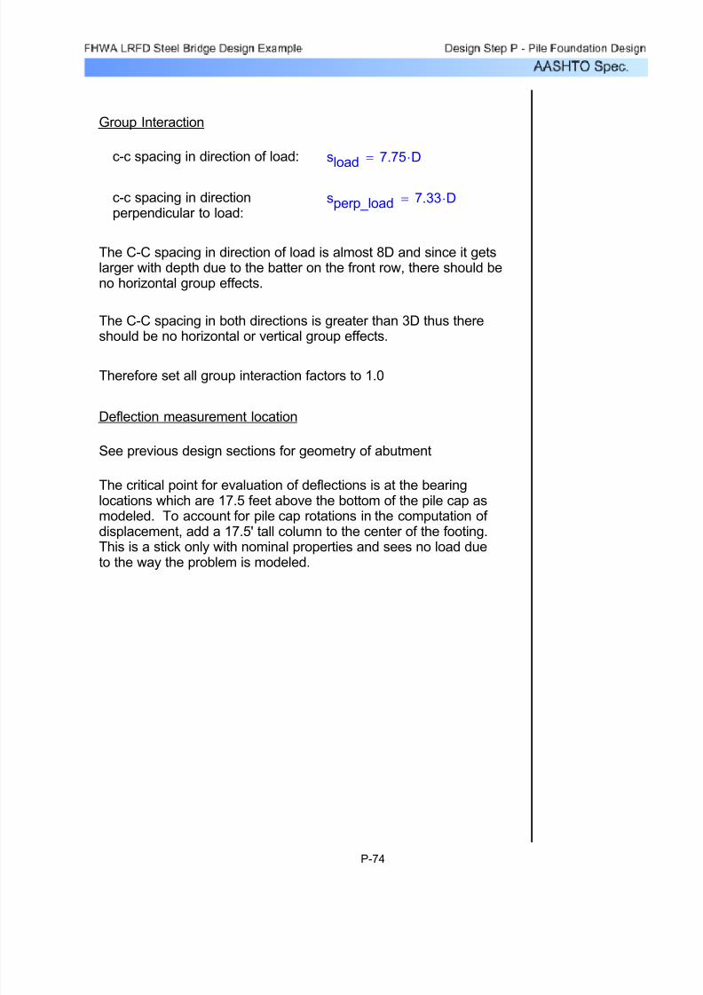
7/29/2019 LRFD steel design.pdf
http://slidepdf.com/reader/full/lrfd-steel-designpdf 605/646
Group Interaction
c-c spacing in direction of load: sload 7.75 D⋅=
c-c spacing in directionperpendicular to load:
sperp_load 7.33 D⋅=
The C-C spacing in direction of load is almost 8D and since it getslarger with depth due to the batter on the front row, there should beno horizontal group effects.
The C-C spacing in both directions is greater than 3D thus thereshould be no horizontal or vertical group effects.
Therefore set all group interaction factors to 1.0
Deflection measurement location
See previous design sections for geometry of abutment
The critical point for evaluation of deflections is at the bearinglocations which are 17.5 feet above the bottom of the pile cap as
modeled. To account for pile cap rotations in the computation of displacement, add a 17.5' tall column to the center of the footing.This is a stick only with nominal properties and sees no load dueto the way the problem is modeled.
P-74
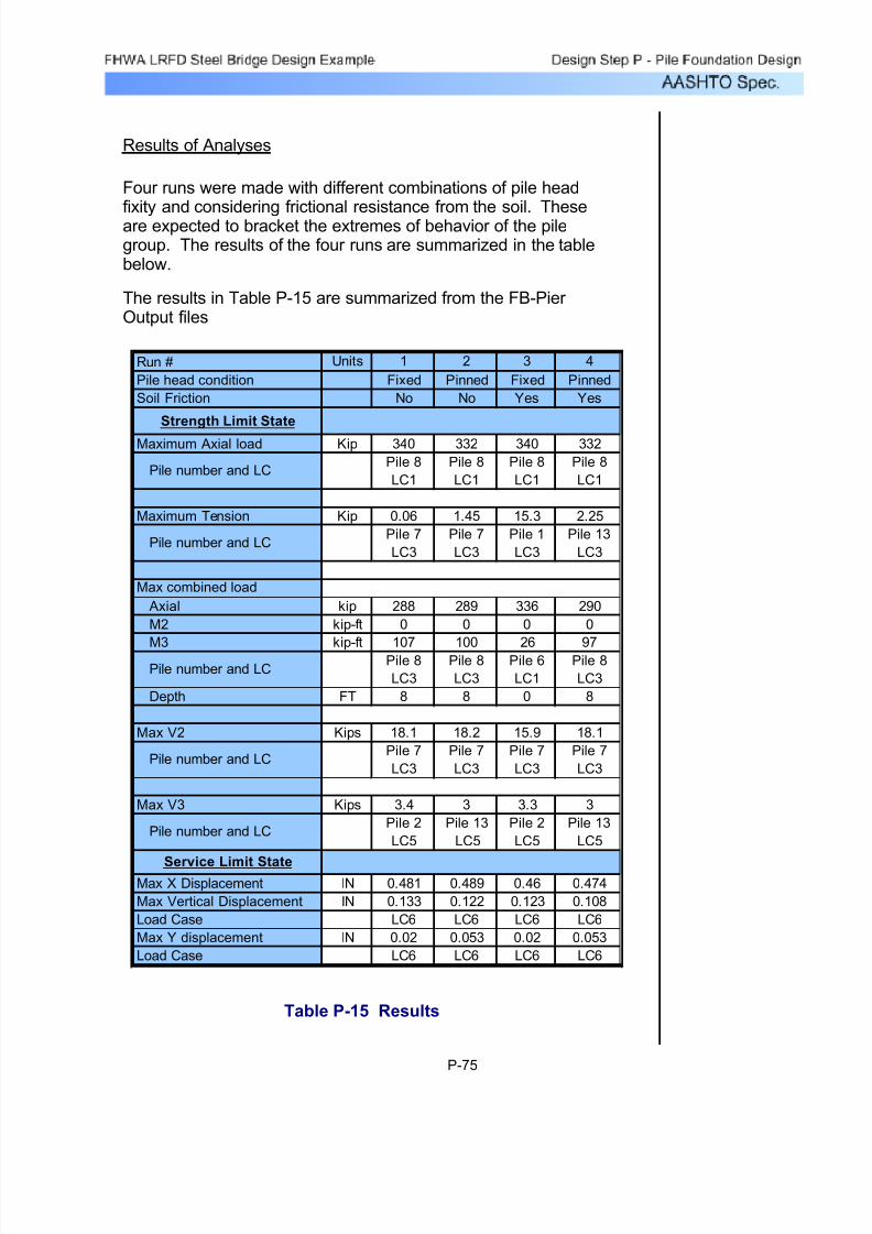
7/29/2019 LRFD steel design.pdf
http://slidepdf.com/reader/full/lrfd-steel-designpdf 606/646
Results of Analyses
Four runs were made with different combinations of pile headfixity and considering frictional resistance from the soil. Theseare expected to bracket the extremes of behavior of the pilegroup. The results of the four runs are summarized in the tablebelow.
The results in Table P-15 are summarized from the FB-Pier Output files
Units 1 2 3 4
Fixed Pinned Fixed Pinned
No No Yes Yes
Kip 340 332 340 332
Pile 8
LC1
Pile 8
LC1
Pile 8
LC1
Pile 8
LC1
Kip 0.06 1.45 15.3 2.25
Pile 7
LC3
Pile 7
LC3
Pile 1
LC3
Pile 13
LC3
kip 288 289 336 290
kip-ft 0 0 0 0
kip-ft 107 100 26 97Pile 8
LC3
Pile 8
LC3
Pile 6
LC1
Pile 8
LC3
FT 8 8 0 8
Kips 18.1 18.2 15.9 18.1
Pile 7
LC3
Pile 7
LC3
Pile 7
LC3
Pile 7
LC3
Kips 3.4 3 3.3 3
Pile 2
LC5
Pile 13
LC5
Pile 2
LC5
Pile 13
LC5
IN 0.481 0.489 0.46 0.474
IN 0.133 0.122 0.123 0.108
LC6 LC6 LC6 LC6
IN 0.02 0.053 0.02 0.053
LC6 LC6 LC6 LC6
Run #
Pile head condition
Soil Friction
Strength Limit State
Axial
Pile number and LC
Maximum Tension
Maximum Axial load
Pile number and LC
Max V2
Pile number and LC
M2
M3Pile number and LC
Depth
Max X DisplacementService Limit State
Max combined load
Max V3
Pile number and LC
Max Vertical Displacement
Load Case
Max Y displacement
Load Case
Table P-15 Results
P-75
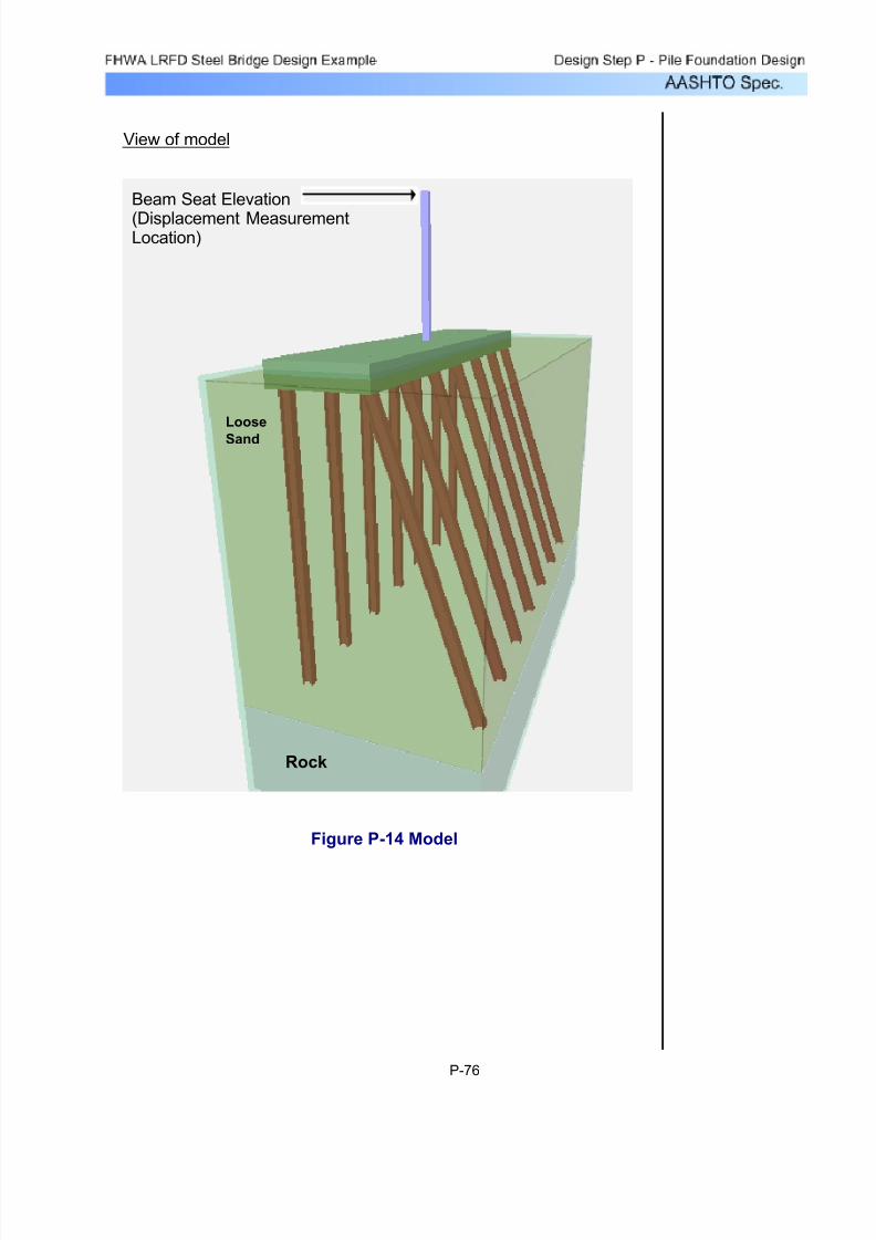
7/29/2019 LRFD steel design.pdf
http://slidepdf.com/reader/full/lrfd-steel-designpdf 607/646
View of model
Beam Seat Elevation
(Displacement MeasurementLocation)
Loose
Sand
Rock
Figure P-14 Model
P-76
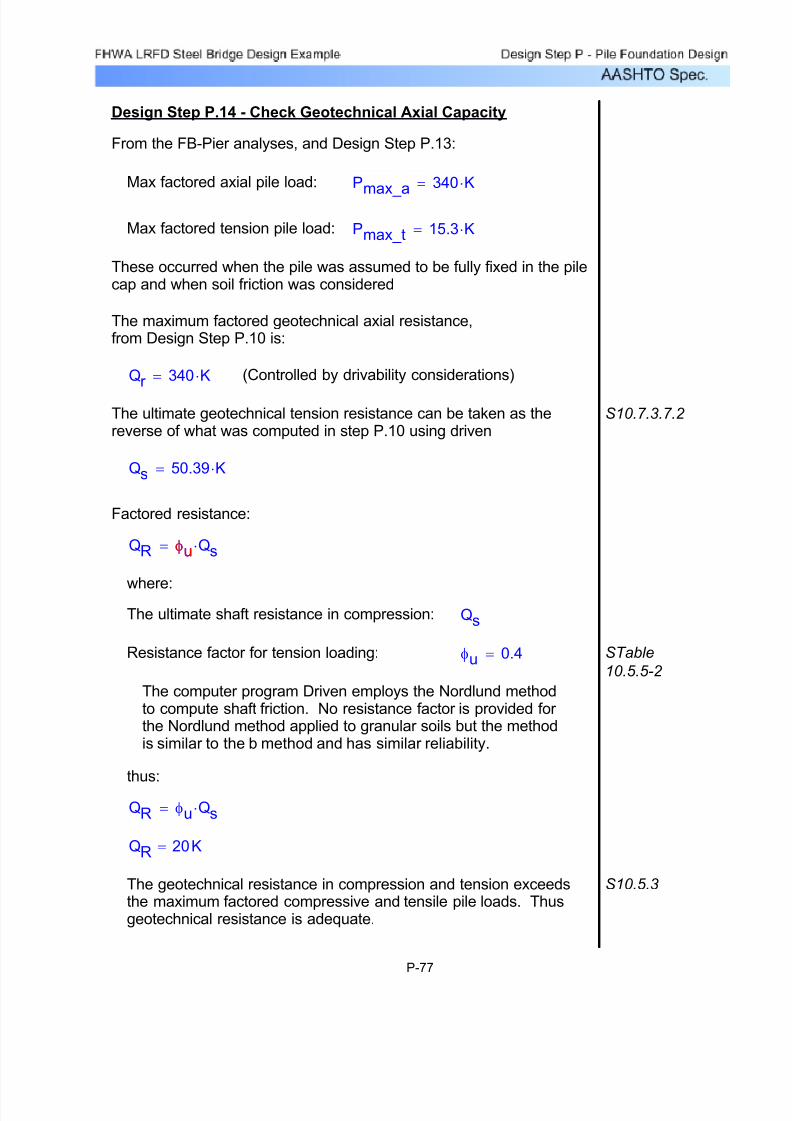
7/29/2019 LRFD steel design.pdf
http://slidepdf.com/reader/full/lrfd-steel-designpdf 608/646
S10.5.3The geotechnical resistance in compression and tension exceedsthe maximum factored compressive and tensile pile loads. Thusgeotechnical resistance is adequate.
QR 20K=
QR φu Qs⋅=
thus:
The computer program Driven employs the Nordlund methodto compute shaft friction. No resistance factor is provided for the Nordlund method applied to granular soils but the methodis similar to the b method and has similar reliability.
STable
10.5.5-2 φu 0.4=Resistance factor for tension loading:
QsThe ultimate shaft resistance in compression:
where:
QR φu Qs⋅= φu
Factored resistance:
Qs 50.39 K⋅=
S10.7.3.7.2 The ultimate geotechnical tension resistance can be taken as thereverse of what was computed in step P.10 using driven
(Controlled by drivability considerations)Qr 340 K⋅=
The maximum factored geotechnical axial resistance,from Design Step P.10 is:
These occurred when the pile was assumed to be fully fixed in the pilecap and when soil friction was considered
Pmax_t 15.3 K⋅=Max factored tension pile load:
P
max_a
340 K⋅=Max factored axial pile load:
From the FB-Pier analyses, and Design Step P.13:
Design Step P.14 - Check Geotechnical Axial Capacity
P-77

7/29/2019 LRFD steel design.pdf
http://slidepdf.com/reader/full/lrfd-steel-designpdf 609/646
Design Step P.15 - Check Structural Axial Capacity
(in lower portion of pile)
From the FB-Pier analyses, and Design Step P.13:
Max factored axial pile load: Pmax_a 340 K⋅=
Max factored tension pile load: Pmax_t 15.3 K⋅=
These occurred when the pile was assumed to be fully fixed in the pilecap and when soil friction was considered
The maximum factored structural axial resistance in the lower portionof the pile, from Design Step P.10 is:
Pr 465K=
This is also applicable to tension.
The factored structural resistance far exceeds the maximum factoredloads. Thus, the piles are adequately sized to transmit axial loads.
P-78
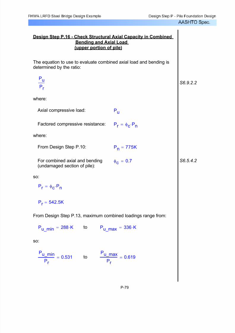
7/29/2019 LRFD steel design.pdf
http://slidepdf.com/reader/full/lrfd-steel-designpdf 610/646
Pu_max
Pr
0.619=toPu_min
Pr
0.531=
so:
Pu_max 336 K⋅=toPu_min 288 K⋅=
From Design Step P.13, maximum combined loadings range from:
Pr 542.5K=
Pr φc Pn⋅=
so:
S6.5.4.2 φc 0.7=For combined axial and bending(undamaged section of pile):
Pn 775K=From Design Step P.10:
where:
Pr φc Pn⋅=Factored compressive resistance:
Pu Axial compressive load:
where:
S6.9.2.2 Pu
Pr
The equation to use to evaluate combined axial load and bending isdetermined by the ratio:
Design Step P.16 - Check Structural Axial Capacity in Combined
Bending and Axial Load
(upper portion of pile)
P-79

7/29/2019 LRFD steel design.pdf
http://slidepdf.com/reader/full/lrfd-steel-designpdf 611/646
Mn is computed in accordance with the provisions of Section 6.12.
S6.5.4.2 φf 1.0=The resistance factor for combined bendingand axial load in piles:
where:
S6.10.4-1Mr φf Mn⋅= Mn
Flexural resistance is:
MryFactored flexural resistance about the y axis:
MrxFactored flexural resistance about the x axis:
MuyFactored flexural moment about the y axis,from Design Step P.13:
MuxFactored flexural moment about the x axis,from Design Step P.13:
are as defined abovePu Pr ,
where:
SEquation
6.9.2.2-2
Pu
Pr
8
9
Mux
Mrx
Muy
Mry
+⎛
⎝
⎞
⎠⋅+ 1.0≤
The combined loading must satisfy:
Since these are both greater than 0.2
P-80

7/29/2019 LRFD steel design.pdf
http://slidepdf.com/reader/full/lrfd-steel-designpdf 612/646
3.76E
Fyc
⎛
⎝
⎞
⎠
0.5
⋅ 90.553=2 Dcp⋅
tw
25.08=
Check:
Fyc 50 ksi⋅= As in Design Step P.10:
E 29000 ksi⋅=Modulus of Elasticity:
tw 0.435in=From Design Step P.5:
Dcp 5.455 in⋅=Dcpd
2 tf −=
2 tf −
for HP 12 x 53 Grade 50 piles:
SEquation
6.10.4.1.2-1
2 Dcp⋅
tw
3.76E
Fyc
⎛
⎝
⎞
⎠
0.5
⋅≤
Criteria from Section 6.10.4.1.2:
S6.12.2.2.1For bending about the x axis, the provisions of Section 6.10.4 applyas follows:
Deep Foundations Surrounded by Soil
In most cases where deep foundations are completely
surrounded by soil, lateral support from even theweakest soil is sufficient such that the unbraced lengthcan be considered zero. When the unbraced length iszero, the buckling considerations of section 6.10.4generally result in no reduction of the ultimate bendingstress and Mn=the plastic moment or Mn=f y*Z where Zis the plastic section modulus. Note that the plasticsection modulus is used in LRFD design, not theelastic section modulus. The evaluation of bucklingcriteria on the following pages is presented for completeness.
P-81
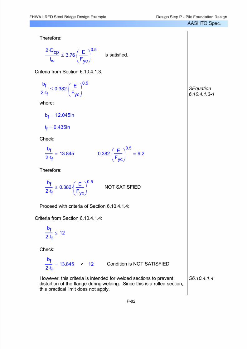
7/29/2019 LRFD steel design.pdf
http://slidepdf.com/reader/full/lrfd-steel-designpdf 613/646
S6.10.4.1.4However, this criteria is intended for welded sections to preventdistortion of the flange during welding. Since this is a rolled section,this practical limit does not apply.
Condition is NOT SATISFIED12>bf
2 tf ⋅13.845=
Check:
bf
2 tf ⋅12≤
Criteria from Section 6.10.4.1.4:
Proceed with criteria of Section 6.10.4.1.4:
NOT SATISFIEDbf
2 tf ⋅0.382 E
Fyc
⎛ ⎝
⎞ ⎠
0.5⋅≤
Therefore:
0.382E
Fyc
⎛
⎝
⎞
⎠
0.5
⋅ 9.2=bf
2 tf ⋅13.845=
Check:
tf 0.435in=
bf 12.045in=
where:
SEquation
6.10.4.1.3-1
bf
2 tf ⋅0.382
E
Fyc
⎛
⎝
⎞
⎠
0.5
⋅≤
Criteria from Section 6.10.4.1.3:
is satisfied.2 Dcp⋅
tw
3.76E
Fyc
⎛
⎝
⎞
⎠
0.5
⋅≤
Therefore:
P-82

7/29/2019 LRFD steel design.pdf
http://slidepdf.com/reader/full/lrfd-steel-designpdf 614/646
RbLoad shedding factor specified inSection 6.10.4.3.2:
S6.10.4.3.1aRh 1.0=Hybrid factor as specified in Section6.10.4.3.1 for a homogeneous section:
and:
Fcr 50 ksi⋅=
so:
Fyc 50ksi=cannot exceedFcr
but:
Fcr
57.52ksi=
Fcr 1.904 E⋅
bf
2 tf ⋅
⎛
⎝
⎞
⎠
22 Dcp⋅
tw
⎛
⎝
⎞
⎠
0.5
⋅
=
where:
SEquation
6.10.4.2.4a-2
F
n
R
b
R
h
⋅ F
cr
⋅= F
cr
For compression flange:
Proceed to noncompact section flange flexural resistance of Section 6.10.4.2.4
S6.10.4.1.9The pile is laterally braced along its entire length by the adjacent soilthus the unbraced length (Lb) is zero and this condition is alwayssatisfied.
Criteria from Section 6.10.4.1.9:
Therefore proceed to bracing requirements of Section 6.10.4.1.9:
P-83
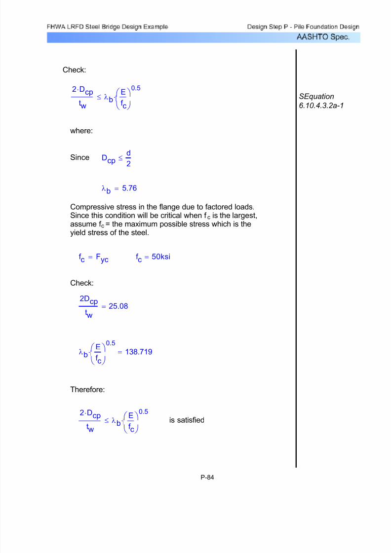
7/29/2019 LRFD steel design.pdf
http://slidepdf.com/reader/full/lrfd-steel-designpdf 615/646
is satisfied2 Dcp⋅
tw
λbE
f c
⎛
⎝
⎞
⎠
0.5
⋅≤
Therefore:
λbE
f c
⎛
⎝
⎞
⎠
0.5
⋅ 138.719=
2Dcp
tw
25.08=
Check:
f c 50ksi=f c Fyc=
Compressive stress in the flange due to factored loads.Since this condition will be critical when f c is the largest,assume f c = the maximum possible stress which is theyield stress of the steel.
λb
5.76=
Dcpd
2≤Since
where:
SEquation6.10.4.3.2a-1
2 Dcp⋅
twλb
E
f c⎛ ⎝ ⎞ ⎠
0.5
⋅≤
Check:
P-84

7/29/2019 LRFD steel design.pdf
http://slidepdf.com/reader/full/lrfd-steel-designpdf 616/646
Mp Fy Zx⋅=
Mn Mp= Mp
Since the nominal plastic stress in all components of the pile isequal to the yield stress, The nominal moment capacity may be
computed as the plastic moment.
Fn 50ksi=
Fn Rb Rh⋅ Fyt⋅=
Therefore:
F
yt
50 ksi⋅=
S6.10.4.3.2bfor tension flangeRb 1=
Rh 1=
where:
SEquation6.10.4.2b-1
Fn Rb Rh⋅ Fyt⋅= Fyt
For tension flange:
Fn 50ksi=
Fn Rb Rh⋅ Fcr ⋅=
so:
Rb 1.0=
thus:
P-85
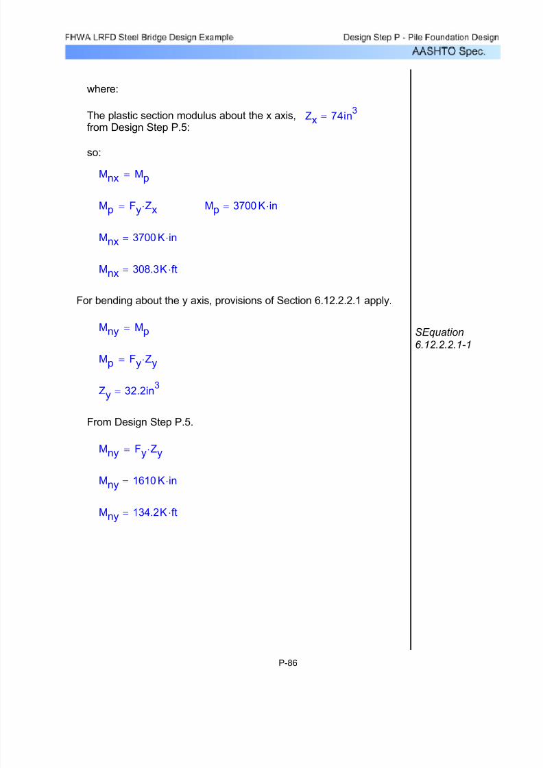
7/29/2019 LRFD steel design.pdf
http://slidepdf.com/reader/full/lrfd-steel-designpdf 617/646
Mny 134.2K ft⋅=
Mny 1610 K in⋅=
Mny Fy Zy⋅=
From Design Step P.5.
Zy 32.2in3=
Mp Fy Zy⋅=
SEquation
6.12.2.2.1-1
Mny Mp=
For bending about the y axis, provisions of Section 6.12.2.2.1 apply.
Mnx 308.3K ft⋅=
Mnx 3700 K in⋅=
Mp 3700 K in⋅=Mp Fy Zx⋅=
Mnx Mp=
so:
Zx 74in3=The plastic section modulus about the x axis,
from Design Step P.5:
where:
P-86
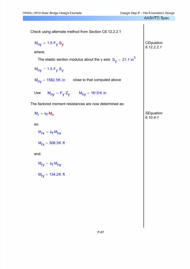
7/29/2019 LRFD steel design.pdf
http://slidepdf.com/reader/full/lrfd-steel-designpdf 618/646
Mry 134.2K ft⋅=
Mry φf Mny⋅=
and:
Mrx 308.3K ft⋅=
Mrx φf Mnx⋅=
so:
SEquation
6.10.4-1Mr φf Mn⋅= Mn
The factored moment resistances are now determined as:
Mny 1610 K in⋅=Mny Fy Zy⋅=Use
close to that computed aboveMny 1582.5K in⋅=
Mny 1.5 Fy⋅ Sy⋅=
Sy 21.1 in3⋅=The elastic section modulus about the y axis:
where:
CEquation
6.12.2.2.1
Mny 1.5 Fy⋅ Sy⋅= Sy
Check using alternate method from Section C6.12.2.2.1
P-87

7/29/2019 LRFD steel design.pdf
http://slidepdf.com/reader/full/lrfd-steel-designpdf 619/646
From the maximum combined loads from Design Step P.13:
The interaction equation is now applied to the maximum combinedloading conditions determined in the 4 FB-Pier analyses as follows
Pu
542.5
8
9
Mux
308.3
Muy
134.2+
⎛
⎝
⎞
⎠⋅+ 1.0≤ SEquation
6.9.2.2-2
FB-Pier
Run #
Pu
(kips)
Mux
(kip-ft)
Muy
(kip-ft)
1 288 107 0
2 289 100 0
3 336 26 04 290 97 0 0.81
Results of interaction
equation
0.84
0.82
0.69
Table P-16 Results of Interaction Equation
All conditions satisfy the interaction equation thus piles areacceptable under combined loading.
P-88

7/29/2019 LRFD steel design.pdf
http://slidepdf.com/reader/full/lrfd-steel-designpdf 620/646
and
Vp 148.6K=
Vp 0.58 Fyw⋅ D⋅ tw⋅=
so:
tw 0.435in=
D 11.78 in⋅=
From Design Step P.5
Fyw 50 ksi⋅=
SEquation
6.10.7.2-2 Vp 0.58 Fyw⋅ D⋅ tw⋅= Fyw
where:
SEquation
6.10.7.2-1Vn C Vp⋅= Vp
The nominal shear capacity of the pile section is computed as for anunstiffened web of a steel beam.
Pile Capacity
The capacity of the pile section to resist the maximumapplied shear force is usually not critical for steel pilesections placed in groups such that high overturningmoments are not required to be resisted by the pile.However, in foundation systems consisting of concretefoundation elements arranged as a single element or asingle row of elements supporting a tall laterally loadedpier or supporting a column subject to a largeeccentric vertical load, this can become the controllingcriteria. It is checked here for completeness.
Design Step P.17 - Check Structural Shear Capacity
P-89

7/29/2019 LRFD steel design.pdf
http://slidepdf.com/reader/full/lrfd-steel-designpdf 621/646
Thus, piles are acceptable for shear.
From Design Step P.13, the maximum factored shear in anypile in the FB-Pier analysis was 18.2 K.
Vr 148.6K=
Vr φv Vn⋅=
so:
S6.5.4.2 φv 1.0=Resistance factor for shear:
Vr φv Vn⋅= φvFactored resistance:
Vn 148.6K=
Vn C Vp⋅=
so:
C 1.0=thus:
27.08 59.237<Check:
1.129000 5⋅
50
⎛
⎝
⎞
⎠
0.5
⋅ 59.237=
SEquation
6.10.7.3.3a-5 1.1
E k⋅
Fyw
⎛
⎝
⎞
⎠
0.5
⋅compute:
Dtw
27.08=compute:
C is determined based on criteria in Section 6.10.7.3.3awith k = 5
P-90

7/29/2019 LRFD steel design.pdf
http://slidepdf.com/reader/full/lrfd-steel-designpdf 622/646
S10.7.2.4 and
S10.7.2.3.1
Thus deflections are within tolerances and Service limit statesare satisfied.
S10.7.2.3.1∆v_all 0.5 in⋅=The maximum vertical deflection allowed is
S10.7.2.2 ∆h_all 1.5 in⋅=The maximum horizontal deflection allowed is
The structural engineer has determined allowable deflections as
∆v 0.133 in⋅=The maximum vertical deflection observed is
∆h 0.489 in⋅=The maximum horizontal deflection observed is
From Design Step P.13:
It can be seen from the results that the horizontal displacements at thebeam seat elevation are slightly higher for the cases of pinned headpiles. This is expected and the difference is usually much greater. Inthis case, the battered piles in the front row resist the majority of thelateral load so pile head fixity is not critical to performance of thefoundation system.
Displacements were determined in the interaction analysis with FB-Pier
Design Step P.18 - Check Maximum Horizontal and Vertical
Deflection of Pile Group at Beam Seats
Using Service Load Case
P-91
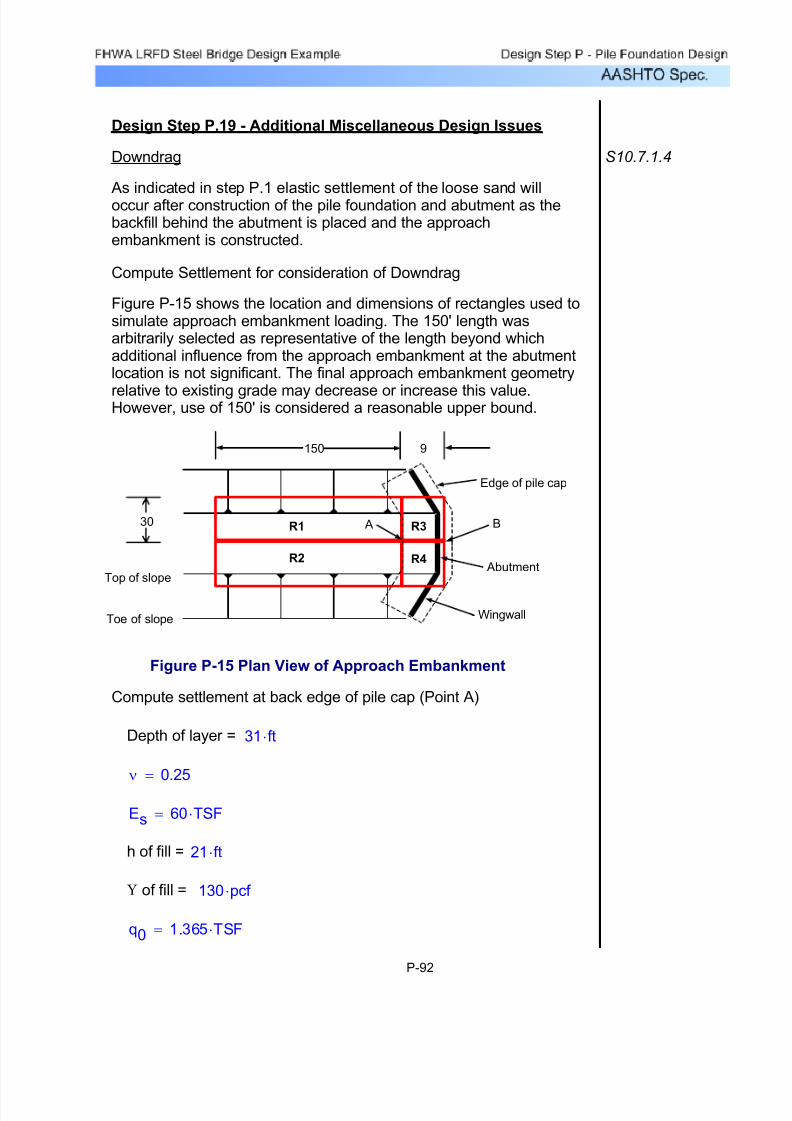
7/29/2019 LRFD steel design.pdf
http://slidepdf.com/reader/full/lrfd-steel-designpdf 623/646
q0 1.365 TSF⋅=
130 pcf ⋅Υ of fill =
21 ft⋅h of fill =
Es 60 TSF⋅=
ν 0.25=
31 ft⋅Depth of layer =
Compute settlement at back edge of pile cap (Point A)
Figure P-15 Plan View of Approach Embankment
150 9
30 B A
Edge of pile cap
Abutment
WingwallToe of slope
Top of slope
R1
R2 R4
R3
Figure P-15 shows the location and dimensions of rectangles used tosimulate approach embankment loading. The 150' length wasarbitrarily selected as representative of the length beyond whichadditional influence from the approach embankment at the abutmentlocation is not significant. The final approach embankment geometry
relative to existing grade may decrease or increase this value.However, use of 150' is considered a reasonable upper bound.
Compute Settlement for consideration of Downdrag
As indicated in step P.1 elastic settlement of the loose sand willoccur after construction of the pile foundation and abutment as thebackfill behind the abutment is placed and the approachembankment is constructed.
S10.7.1.4Downdrag
Design Step P.19 - Additional Miscellaneous Design Issues
P-92
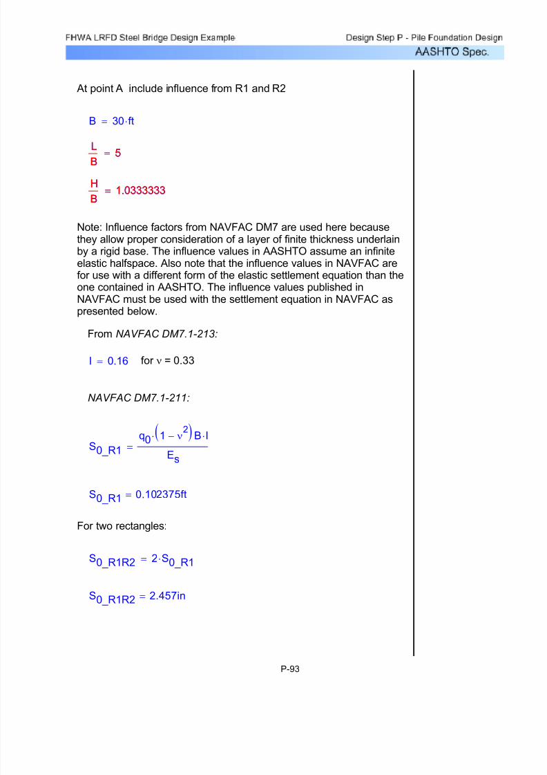
7/29/2019 LRFD steel design.pdf
http://slidepdf.com/reader/full/lrfd-steel-designpdf 624/646
At point A include influence from R1 and R2
B 30 ft⋅=
L
B5=
L
B5=
H
B1.0333333=
H
B1.0333333=
Note: Influence factors from NAVFAC DM7 are used here becausethey allow proper consideration of a layer of finite thickness underlainby a rigid base. The influence values in AASHTO assume an infiniteelastic halfspace. Also note that the influence values in NAVFAC arefor use with a different form of the elastic settlement equation than theone contained in AASHTO. The influence values published inNAVFAC must be used with the settlement equation in NAVFAC aspresented below.
From NAVFAC DM7.1-213:
I 0.16= for ν = 0.33
NAVFAC DM7.1-211:
S0_R1
q0 1 ν2
−( )⋅ B I⋅
Es
=
S0_R1 0.102375ft=
For two rectangles:
S0_R1R2 2 S0_R1⋅=
S0_R1R2 2.457in=
P-93

7/29/2019 LRFD steel design.pdf
http://slidepdf.com/reader/full/lrfd-steel-designpdf 625/646
S0_R1R2 S0_R3R4− 0.383906in=
S0_R1R2 S0_R3R4− 0.031992ft=
R1 R2+ R3 R4+( )− S0_R1R2 S0_R3R4−=R1 R2+ R3 R4+( )− S0_R1R2 S0_R3R4−=
(for two rectangles)S0_R3R4 0.172758ft=
S0_R3R4 2 S0_R3⋅=
S0_R3
q0 1 ν2
−( )⋅ B I⋅
Es
=
for ν = 0.33I 0.45=
From NAVFAC DM7.1-213
H
B3.444444=
H
B3.444444=
LB
3.333333=LB
3.333333=
B 9 ft⋅=
Contribution of R3 and R4 only
To simulate this case; the corner of R1 and R2 are shifted forward tobe coincident with point B, and the settlement due to the approach fillweight will be equal to that computed for Point A. However, theweight of the approach embankment above the heel of the footingwill be supported by the pile foundation and will not contribute toelastic settlement. Thus the settlement at point B can be computedby subtracting the influence of rectangles R3 and R4 from thesettlement computed for rectangles R1 and R2 alone.
Compute settlement at front row of piles (Point B)
P-94
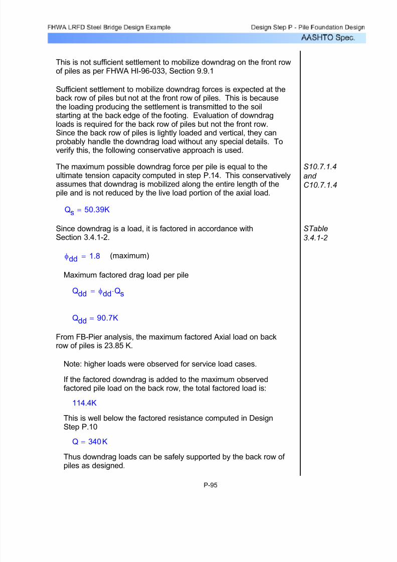
7/29/2019 LRFD steel design.pdf
http://slidepdf.com/reader/full/lrfd-steel-designpdf 626/646
Thus downdrag loads can be safely supported by the back row of piles as designed.
Q 340K=
This is well below the factored resistance computed in DesignStep P.10
114.4K
If the factored downdrag is added to the maximum observedfactored pile load on the back row, the total factored load is:
Note: higher loads were observed for service load cases.
From FB-Pier analysis, the maximum factored Axial load on backrow of piles is 23.85 K.
Qdd 90.7K=
Qdd
φdd
Qs
⋅=
Maximum factored drag load per pile
(maximum)φdd 1.8=
STable
3.4.1-2
Since downdrag is a load, it is factored in accordance withSection 3.4.1-2.
Qs 50.39K=
S10.7.1.4
and
C10.7.1.4
The maximum possible downdrag force per pile is equal to theultimate tension capacity computed in step P.14. This conservativelyassumes that downdrag is mobilized along the entire length of the
pile and is not reduced by the live load portion of the axial load.
Sufficient settlement to mobilize downdrag forces is expected at the
back row of piles but not at the front row of piles. This is becausethe loading producing the settlement is transmitted to the soilstarting at the back edge of the footing. Evaluation of downdragloads is required for the back row of piles but not the front row.Since the back row of piles is lightly loaded and vertical, they canprobably handle the downdrag load without any special details. Toverify this, the following conservative approach is used.
This is not sufficient settlement to mobilize downdrag on the front rowof piles as per FHWA HI-96-033, Section 9.9.1
P-95
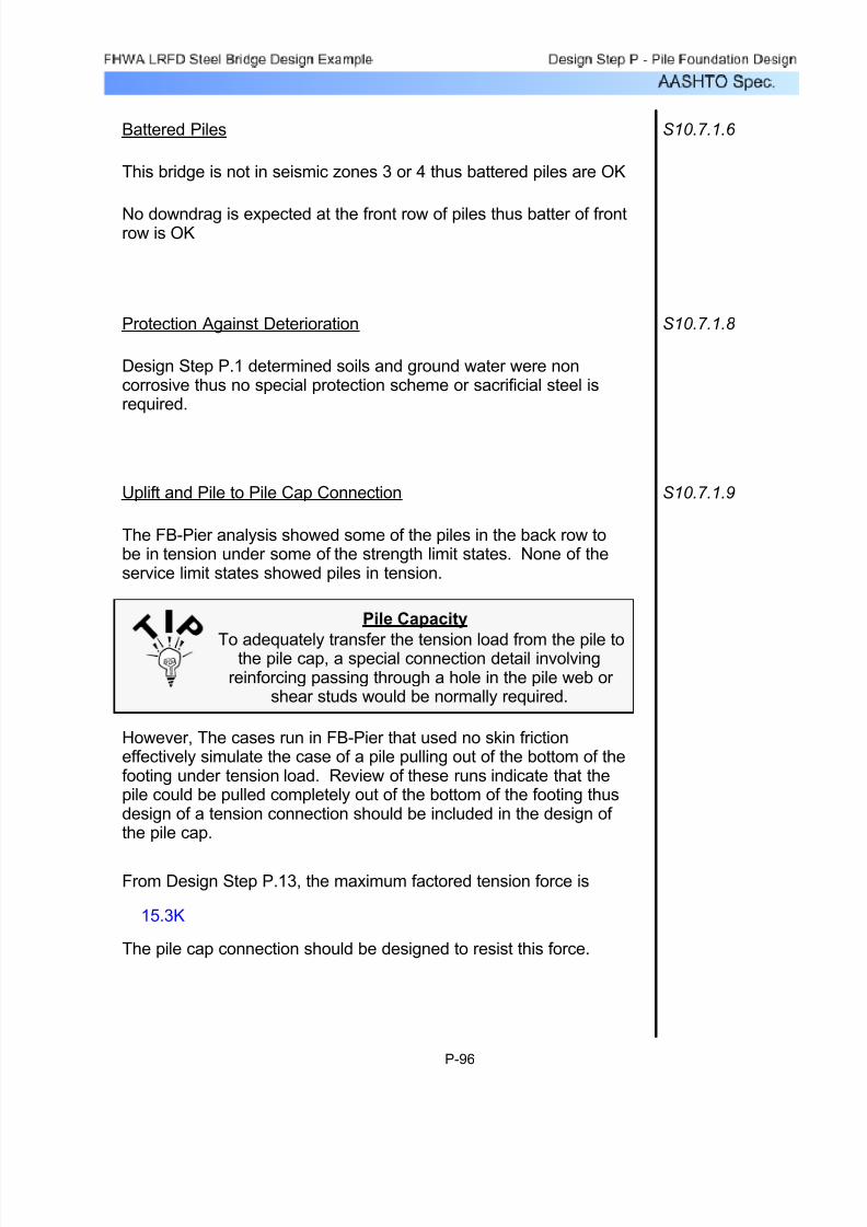
7/29/2019 LRFD steel design.pdf
http://slidepdf.com/reader/full/lrfd-steel-designpdf 627/646
The pile cap connection should be designed to resist this force.
15.3K
From Design Step P.13, the maximum factored tension force is
However, The cases run in FB-Pier that used no skin frictioneffectively simulate the case of a pile pulling out of the bottom of thefooting under tension load. Review of these runs indicate that thepile could be pulled completely out of the bottom of the footing thusdesign of a tension connection should be included in the design of the pile cap.
Pile Capacity
To adequately transfer the tension load from the pile tothe pile cap, a special connection detail involvingreinforcing passing through a hole in the pile web or
shear studs would be normally required.
The FB-Pier analysis showed some of the piles in the back row tobe in tension under some of the strength limit states. None of theservice limit states showed piles in tension.
S10.7.1.9Uplift and Pile to Pile Cap Connection
Design Step P.1 determined soils and ground water were noncorrosive thus no special protection scheme or sacrificial steel isrequired.
S10.7.1.8 Protection Against Deterioration
No downdrag is expected at the front row of piles thus batter of frontrow is OK
This bridge is not in seismic zones 3 or 4 thus battered piles are OK
S10.7.1.6 Battered Piles
P-96
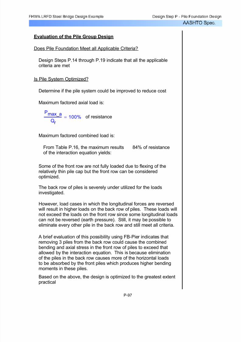
7/29/2019 LRFD steel design.pdf
http://slidepdf.com/reader/full/lrfd-steel-designpdf 628/646
Based on the above, the design is optimized to the greatest extentpractical
A brief evaluation of this possibility using FB-Pier indicates thatremoving 3 piles from the back row could cause the combinedbending and axial stress in the front row of piles to exceed thatallowed by the interaction equation. This is because eliminationof the piles in the back row causes more of the horizontal loadsto be absorbed by the front piles which produces higher bendingmoments in these piles.
However, load cases in which the longitudinal forces are reversedwill result in higher loads on the back row of piles. These loads willnot exceed the loads on the front row since some longitudinal loadscan not be reversed (earth pressure). Still, it may be possible toeliminate every other pile in the back row and still meet all criteria.
The back row of piles is severely under utilized for the loadsinvestigated.
Some of the front row are not fully loaded due to flexing of therelatively thin pile cap but the front row can be consideredoptimized.
84% of resistanceFrom Table P.16, the maximum resultsof the interaction equation yields:
Maximum factored combined load is:
of resistancePmax_a
Qr 100%=
Maximum factored axial load is:
Determine if the pile system could be improved to reduce cost
Is Pile System Optimized?
Design Steps P.14 through P.19 indicate that all the applicablecriteria are met
Does Pile Foundation Meet all Applicable Criteria?
Evaluation of the Pile Group Design
P-97

7/29/2019 LRFD steel design.pdf
http://slidepdf.com/reader/full/lrfd-steel-designpdf 629/646
Summary of Final Design Recommendations
Final Pile Cap Layout
All Piles are HP 12 x 53 Grade 50 All dimensions shown at bottom of pile cap
10' 3"
7' 9"
6 s p a c e s @
7 ' 4 " = 4 4 ' 0 "
4 6 '
1' 5.25"
1' 3"
3.5' 2.75'
CL of pile
cap
STEM
Battered at
1H:3V
Figure P-16 Final Pile Cap Layout
P-98

7/29/2019 LRFD steel design.pdf
http://slidepdf.com/reader/full/lrfd-steel-designpdf 630/646
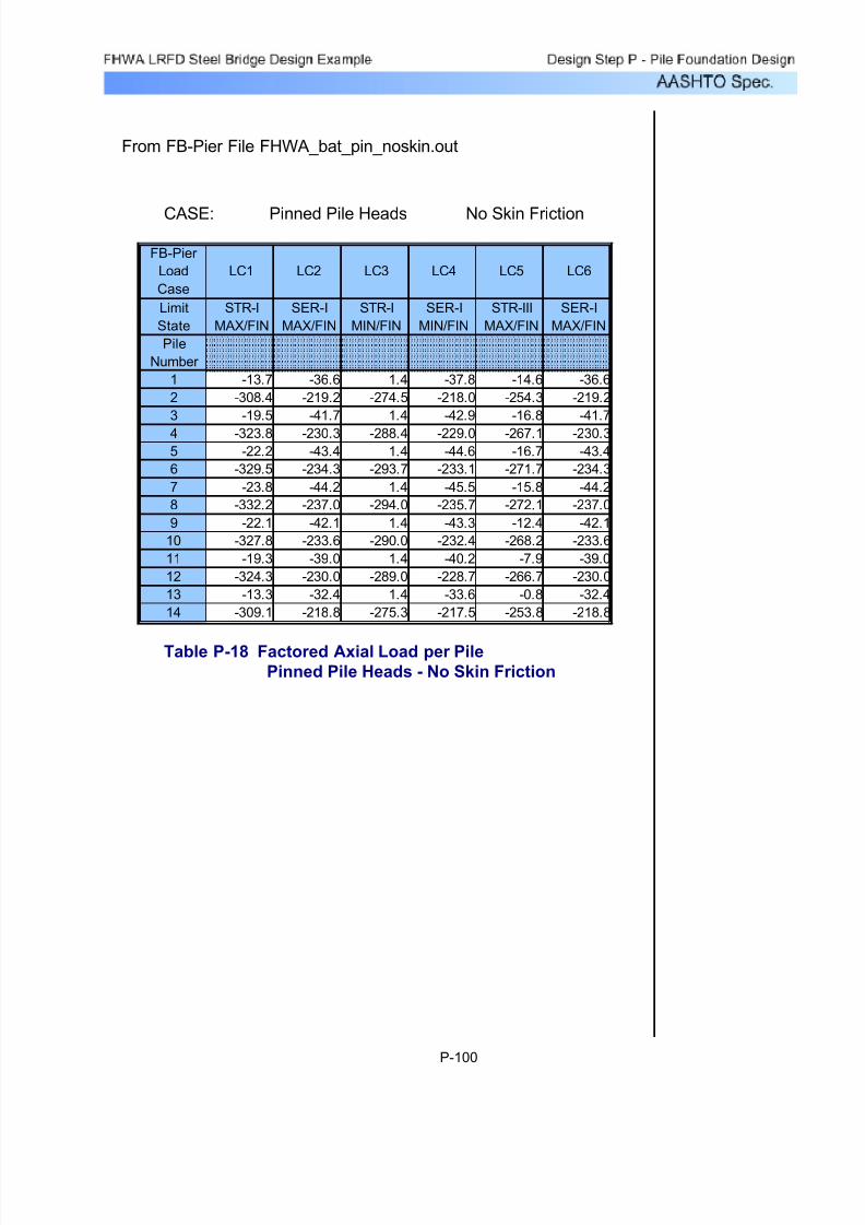
7/29/2019 LRFD steel design.pdf
http://slidepdf.com/reader/full/lrfd-steel-designpdf 631/646
From FB-Pier File FHWA_bat_pin_noskin.out
CASE: Pinned Pile Heads No Skin Friction
FB-Pier
Load
Case
LC1 LC2 LC3 LC4 LC5 LC6
Limit
State
STR-I
MAX/FIN
SER-I
MAX/FIN
STR-I
MIN/FIN
SER-I
MIN/FIN
STR-III
MAX/FIN
SER-I
MAX/FIN
Pile
Number
1 -13.7 -36.6 1.4 -37.8 -14.6 -36.6
2 -308.4 -219.2 -274.5 -218.0 -254.3 -219.2
3 -19.5 -41.7 1.4 -42.9 -16.8 -41.7
4 -323.8 -230.3 -288.4 -229.0 -267.1 -230.3
5 -22.2 -43.4 1.4 -44.6 -16.7 -43.4
6 -329.5 -234.3 -293.7 -233.1 -271.7 -234.3
7 -23.8 -44.2 1.4 -45.5 -15.8 -44.2
8 -332.2 -237.0 -294.0 -235.7 -272.1 -237.0
9 -22.1 -42.1 1.4 -43.3 -12.4 -42.1
10 -327.8 -233.6 -290.0 -232.4 -268.2 -233.6
11 -19.3 -39.0 1.4 -40.2 -7.9 -39.0
12 -324.3 -230.0 -289.0 -228.7 -266.7 -230.0
13 -13.3 -32.4 1.4 -33.6 -0.8 -32.4
14 -309.1 -218.8 -275.3 -217.5 -253.8 -218.8
Table P-18 Factored Axial Load per Pile
Pinned Pile Heads - No Skin Friction
P-100
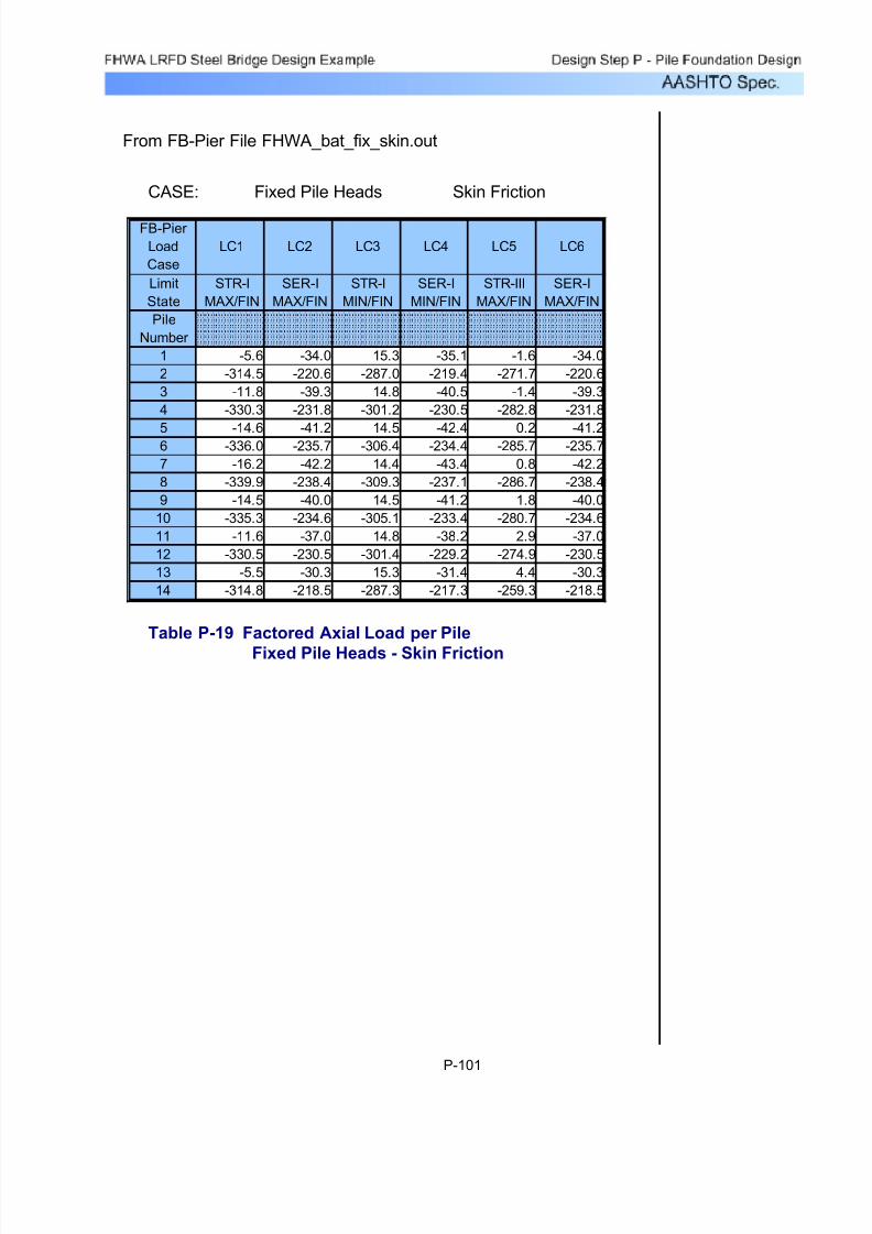
7/29/2019 LRFD steel design.pdf
http://slidepdf.com/reader/full/lrfd-steel-designpdf 632/646
From FB-Pier File FHWA_bat_fix_skin.out
CASE: Fixed Pile Heads Skin Friction
FB-Pier
Load
Case
LC1 LC2 LC3 LC4 LC5 LC6
Limit
State
STR-I
MAX/FIN
SER-I
MAX/FIN
STR-I
MIN/FIN
SER-I
MIN/FIN
STR-III
MAX/FIN
SER-I
MAX/FIN
Pile
Number
1 -5.6 -34.0 15.3 -35.1 -1.6 -34.0
2 -314.5 -220.6 -287.0 -219.4 -271.7 -220.6
3 -11.8 -39.3 14.8 -40.5 -1.4 -39.3
4 -330.3 -231.8 -301.2 -230.5 -282.8 -231.8
5 -14.6 -41.2 14.5 -42.4 0.2 -41.26 -336.0 -235.7 -306.4 -234.4 -285.7 -235.7
7 -16.2 -42.2 14.4 -43.4 0.8 -42.2
8 -339.9 -238.4 -309.3 -237.1 -286.7 -238.4
9 -14.5 -40.0 14.5 -41.2 1.8 -40.0
10 -335.3 -234.6 -305.1 -233.4 -280.7 -234.6
11 -11.6 -37.0 14.8 -38.2 2.9 -37.0
12 -330.5 -230.5 -301.4 -229.2 -274.9 -230.5
13 -5.5 -30.3 15.3 -31.4 4.4 -30.3
14 -314.8 -218.5 -287.3 -217.3 -259.3 -218.5
Table P-19 Factored Axial Load per Pile
Fixed Pile Heads - Skin Friction
P-101
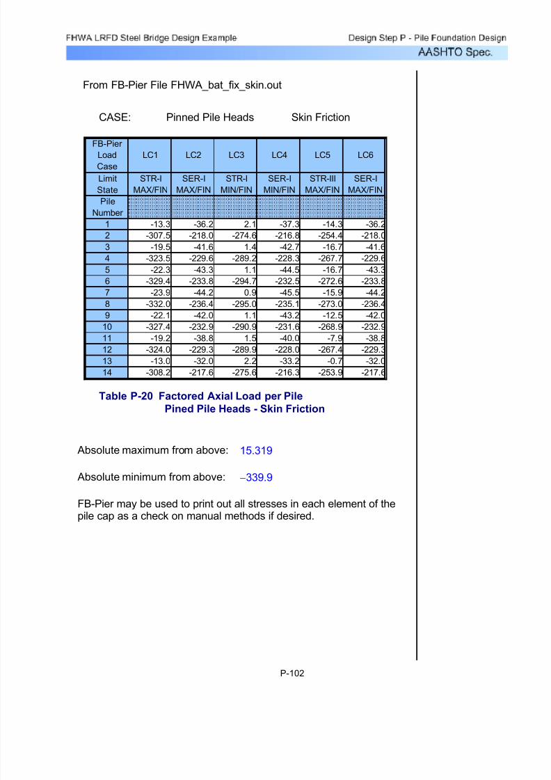
7/29/2019 LRFD steel design.pdf
http://slidepdf.com/reader/full/lrfd-steel-designpdf 633/646
From FB-Pier File FHWA_bat_fix_skin.out
CASE: Pinned Pile Heads Skin Friction
FB-Pier
Load
Case
LC1 LC2 LC3 LC4 LC5 LC6
Limit
State
STR-I
MAX/FIN
SER-I
MAX/FIN
STR-I
MIN/FIN
SER-I
MIN/FIN
STR-III
MAX/FIN
SER-I
MAX/FIN
Pile
Number
1 -13.3 -36.2 2.1 -37.3 -14.3 -36.2
2 -307.5 -218.0 -274.6 -216.8 -254.4 -218.0
3 -19.5 -41.6 1.4 -42.7 -16.7 -41.6
4 -323.5 -229.6 -289.2 -228.3 -267.7 -229.6
5 -22.3 -43.3 1.1 -44.5 -16.7 -43.36 -329.4 -233.8 -294.7 -232.5 -272.6 -233.8
7 -23.9 -44.2 0.9 -45.5 -15.9 -44.2
8 -332.0 -236.4 -295.0 -235.1 -273.0 -236.4
9 -22.1 -42.0 1.1 -43.2 -12.5 -42.0
10 -327.4 -232.9 -290.9 -231.6 -268.9 -232.9
11 -19.2 -38.8 1.5 -40.0 -7.9 -38.8
12 -324.0 -229.3 -289.9 -228.0 -267.4 -229.3
13 -13.0 -32.0 2.2 -33.2 -0.7 -32.0
14 -308.2 -217.6 -275.6 -216.3 -253.9 -217.6
Table P-20 Factored Axial Load per Pile
Pined Pile Heads - Skin Friction
Absolute maximum from above: 15.319
Absolute minimum from above: 339.9−
FB-Pier may be used to print out all stresses in each element of thepile cap as a check on manual methods if desired.
P-102

7/29/2019 LRFD steel design.pdf
http://slidepdf.com/reader/full/lrfd-steel-designpdf 634/646
Design Manual 7; Volume 1 - Soil Mechanics;Volume 2 - Foundations and Earth Structures,Department of the Navy, Naval FacilitiesEngineering Command, May 1982.
NAVFAC DM7
Design and Construction of Driven PileFoundations, Hannigan, P.J., Gobel, G.G,
Thedean, G., Likins, G.E., and Rausche, F.for FHWA, December 1996, Volume 1 and 2
FHWA HI-96-033
References:
This is based on a resistance factor (φ) of 0.65 for piles tested
dynamically.
Qp 523 K⋅=
The ultimate pile point capacity (after subtracting modeled skinfriction) is greater than:
Driving stress is in the range specified above.
Perform a CAPWAP analysis of each dynamically tested pile.The CAPWAP analysis shall confirm the following:
Verify capacity and driving system performance by performingstress wave measurements on a minimum of 2 piles in eachsubstructure. One test shall be on a vertical pile and the other shall
be on a battered pile.
Piles to be driven to absolute refusal defined as a penetrationresistance of 20 Blows Per Inch (BPI) using a hammer and drivingsystem components that produces a driving stress between 37and 45 KSI at refusal. Driving stress to be estimated using waveequation analysis of the selected hammer.
Required Factored Axial Resistance = 340K
Maximum Factored Axial Pile Load = 340K
Notes to be placed on Final Drawing
P-103

7/29/2019 LRFD steel design.pdf
http://slidepdf.com/reader/full/lrfd-steel-designpdf 635/646
PADOT DM4 Design Manual Part 4, PennsylvaniaDepartment of Transportation Publication15M, April 2000
Reese and Wang(1991)
Unpublished paper presenting groupefficiencies of pile groups subject tohorizontal loads in diferent directions and atdifferent spacings.
NCEER-97-0022 Proceedings of the NCEER Workshop onEvaluation of Liquefaction Resistance of Soils, Edited by T.L. Youd, I.M. Idriss.Summary Report, 1997. MCEER Publication
NCEER-97-0022
P-104

7/29/2019 LRFD steel design.pdf
http://slidepdf.com/reader/full/lrfd-steel-designpdf 636/646
Detailed Outline Design Example for a Two-Span Br
FHWA LRFD Steel Design Example
Development of a Comprehensive Design Example
for a Steel Girder Bridge with Commentary
Detailed Outline of Steel Girder Design Example
1. General
1.1 Obtain design criteria
1.1.1 Governing specifications, codes, and standards
1.1.2 Design methodology
1.1.3 Live load requirements1.1.4 Bridge width requirement
1.1.4.1 Number of design lanes (in each direction)
1.1.4.2 Shoulder, sidewalk, and parapet requirements
1.1.4.3 Bridge width1.1.5 Clearance requirements
1.1.5.1 Horizontal clearance1.1.5.2 Vertical clearance
1.1.6 Bridge length requirements
1.1.7 Material properties
1.1.7.1 Deck concrete1.1.7.2 Deck reinforcing steel
1.1.7.3 Structural steel
1.1.7.4 Fasteners1.1.7.5 Substructure concrete
1.1.7.6 Substructure reinforcing steel1.1.8 Future wearing surface requirements1.1.9 Load modifiers
1.1.9.1 Ductility
1.1.9.2 Redundancy1.1.9.3 Operational importance
1.2 Obtain geometry requirements
1.2.1 Horizontal geometry
1.2.1.1 Horizontal curve data1.2.1.2 Horizontal alignment
1.2.2 Vertical geometry
1.2.2.1 Vertical curve data1.2.2.2 Vertical grades
1.3 Span arrangement study
1.3.1 Select bridge type1.3.2 Determine span arrangement
1.3.3 Determine substructure locations
1.3.3.1 Abutments
1.3.3.2 Piers

7/29/2019 LRFD steel design.pdf
http://slidepdf.com/reader/full/lrfd-steel-designpdf 637/646
Detailed Outline Design Example for a Two-Span Br
FHWA LRFD Steel Design Example
1.3.4 Compute span lengths
1.3.5 Check horizontal clearance requirements1.4 Obtain geotechnical recommendations
1.4.1 Develop proposed boring plan
1.4.2 Obtain boring logs
1.4.3 Obtain foundation type recommendations for all substructures1.4.3.1 Abutments
1.4.3.2 Piers
1.4.4 Obtain foundation design parameters1.4.4.1 Allowable bearing pressure
1.4.4.2 Allowable settlement
1.4.4.3 Allowable stability safety factors
• Overturning
• Sliding1.4.4.4 Allowable pile resistance
• Axial
• Lateral1.5 Type, Size and Location (TS&L) study
1.5.1 Select steel girder types1.5.1.1 Composite or noncomposite superstructure
1.5.1.2 Plate girder or roll section
1.5.1.3 Homogeneous or hybrid
1.5.2 Determine girder spacing1.5.3 Determine approximate girder depth
1.5.4 Check vertical clearance requirements
1.6 Plan for bridge aesthetics1.6.1 Function
1.6.2 Proportion1.6.3 Harmony1.6.4 Order and rhythm
1.6.5 Contrast and texture
1.6.6 Light and shadow
2. Concrete Deck Design
2.1 Obtain design criteria2.1.1 Girder spacing
2.1.2 Number of girders
2.1.3 Reinforcing steel cover 2.1.3.1 Top
2.1.3.2 Bottom
2.1.4 Concrete strength2.1.5 Reinforcing steel strength
2.1.6 Concrete density
2.1.7 Future wearing surface
2.1.8 Concrete parapet properties
7/29/2019 LRFD steel design.pdf
http://slidepdf.com/reader/full/lrfd-steel-designpdf 638/646
Detailed Outline Design Example for a Two-Span Br
FHWA LRFD Steel Design Example
2.1.8.1 Weight per unit length
2.1.8.2 Width2.1.8.3 Center of gravity
2.1.9 Design method (assume Strip Method)
2.1.10 Applicable load combinations
2.1.11 Resistance factors2.2 Determine minimum slab thickness
2.2.1 Assume top flange width
2.2.2 Compute effective span length2.3 Determine minimum overhang thickness
2.4 Select thicknesses
2.4.1 Slab2.4.2 Overhang
2.5 Compute dead load effects
2.5.1 Component dead load, DC2.5.2 Wearing surface dead load, DW
2.6 Compute live load effects2.6.1 Dynamic load allowance
2.6.2 Multiple presence factor 2.7 Compute factored positive and negative design moments for each limit state
2.7.1 Service limit states (stress, deformation, and cracking)
2.7.2 Fatigue and fracture limit states (limit cracking)2.7.3 Strength limit states (strength and stability)
2.7.4 Extreme event limit states (e.g., earthquake, vehicular or vessel collision)
2.8 Design for positive flexure in deck 2.9 Check for positive flexure cracking under service limit state
2.10 Design for negative flexure in deck 2.11 Check for negative flexure cracking under service limit state
2.12 Design for flexure in deck overhang
2.12.1 Design overhang for horizontal vehicular collision force2.12.1.1 Check at inside face of parapet
2.12.1.2 Check at design section in overhang
2.12.1.3 Check at design section in first span
2.12.2 Design overhang for vertical collision force2.12.3 Design overhang for dead load and live load
2.12.3.1 Check at design section in overhang
2.12.3.2 Check at design section in first span2.13 Check for cracking in overhang under service limit state
2.14 Compute overhang cut-off length requirement
2.15 Compute overhang development length2.16 Design bottom longitudinal distribution reinforcement
2.17 Design top longitudinal distribution reinforcement
2.18 Design longitudinal reinforcement over piers2.19 Draw schematic of final concrete deck design
3. Steel Girder Design

7/29/2019 LRFD steel design.pdf
http://slidepdf.com/reader/full/lrfd-steel-designpdf 639/646
Detailed Outline Design Example for a Two-Span Br
FHWA LRFD Steel Design Example
3.1 Obtain design criteria3.1.1 Span configuration
3.1.2 Girder configuration
3.1.3 Initial spacing of cross frames
3.1.4 Material properties3.1.5 Deck slab design
3.1.6 Load factors
3.1.7 Resistance factors3.1.8 Multiple presence factors
3.2 Select trial girder section
3.3 Compute section properties3.3.1 Sequence of loading
3.3.2 Effective flange width
3.3.3 Composite or noncomposite3.4 Compute dead load effects
3.4.1 Component dead load, DC3.4.2 Wearing surface dead load, DW
3.5 Compute live load effects3.5.1 Determine live load distribution for moment and shear
3.5.1.1 Interior girders
3.5.1.2 Exterior girders3.5.1.3 Skewed bridges
3.5.2 Dynamic load allowance
3.6 Combine load effects for each limit state3.6.1 Service limit states (stress, deformation, and cracking)
3.6.2 Fatigue and fracture limit states (limit cracking)3.6.3 Strength limit states (strength and stability)
3.6.4 Extreme event limit states (e.g., earthquake, vehicular or vessel collision)
3.7 Check section proportions3.7.1 General proportions
3.7.2 Web slenderness
3.7.3 Flange proportions
3.8 Compute plastic moment capacity (for composite section)3.9 Determine if section is compact or noncompact
3.9.1 Check web slenderness
3.9.2 Check compression flange slenderness (negative flexure only)3.9.3 Check compression flange bracing (negative flexure only)
3.9.4 Check ductility (positive flexure only)
3.9.5 Check plastic forces and neutral axis (positive flexure only)3.10 Design for flexure - strength limit state
3.10.1 Compute design moment
3.10.2 Compute nominal flexural resistance3.10.3 Flexural stress limits for lateral-torsional buckling
3.11 Design for shear (at end panels and at interior panels)
3.11.1 Compute shear resistance

7/29/2019 LRFD steel design.pdf
http://slidepdf.com/reader/full/lrfd-steel-designpdf 640/646
Detailed Outline Design Example for a Two-Span Br
FHWA LRFD Steel Design Example
3.11.2 Check Dc/tw for shear
3.11.3 Check web fatigue stress3.11.4 Check handling requirements
3.11.5 Constructability
3.12 Design transverse intermediate stiffeners
3.12.1 Determine required locations3.12.2 Compute design loads
3.12.3 Select single-plate or double-plate and stiffener sizes
3.12.4 Compute stiffener section properties3.12.4.1 Projecting width
3.12.4.2 Moment of inertia
3.12.4.3 Area3.12.5 Check slenderness requirements
3.12.6 Check stiffness requirements
3.12.7 Check strength requirements3.13 Design longitudinal stiffeners
3.13.1 Determine required locations3.13.2 Compute design loads
3.13.3 Select stiffener sizes3.13.4 Compute stiffener section properties
3.13.4.1 Projecting width
3.13.4.2 Moment of inertia3.13.5 Check slenderness requirements
3.13.6 Check stiffness requirements
3.14 Design for flexure - fatigue and fracture limit state3.14.1 Fatigue load
3.14.2 Load-induced fatigue3.14.2.1 Top flange weld
3.14.2.2 Bottom flange weld
3.14.3 Fatigue requirements for webs3.14.3.1 Flexure
3.14.3.2 Shear
3.14.4 Distortion induced fatigue
3.14.5 Fracture3.15 Design for flexure - service limit state
3.15.1 Optional live load deflection check
3.15.2 Permanent deflection check 3.15.2.1 Compression flange
3.15.2.2 Tension flange
3.16 Design for flexure - constructibility check 3.16.1 Check web slenderness
3.16.2 Check compression flange slenderness
3.16.3 Check compression flange bracing3.17 Check wind effects on girder flanges
3.18 Draw schematic of final steel girder design
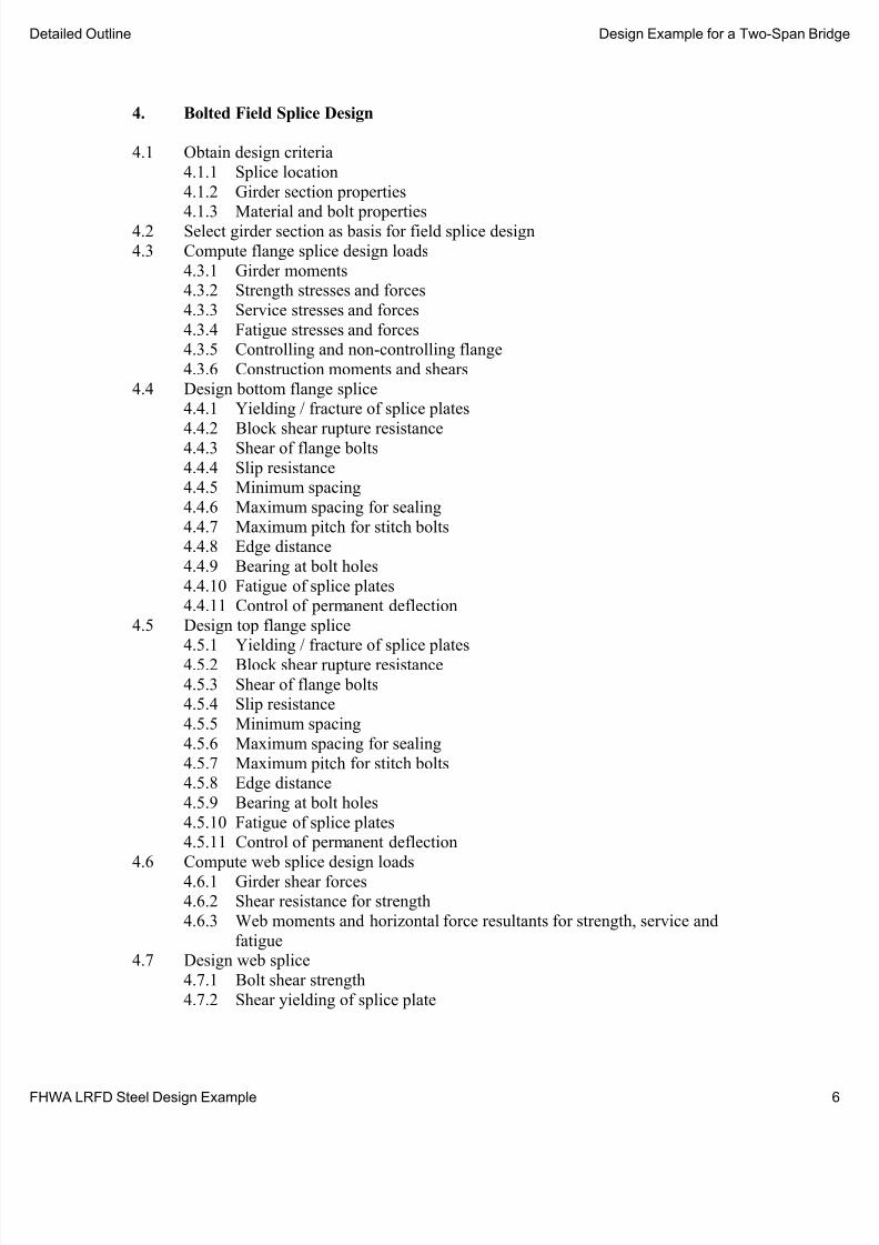
7/29/2019 LRFD steel design.pdf
http://slidepdf.com/reader/full/lrfd-steel-designpdf 641/646
Detailed Outline Design Example for a Two-Span Br
FHWA LRFD Steel Design Example
4. Bolted Field Splice Design
4.1 Obtain design criteria
4.1.1 Splice location
4.1.2 Girder section properties
4.1.3 Material and bolt properties4.2 Select girder section as basis for field splice design
4.3 Compute flange splice design loads
4.3.1 Girder moments4.3.2 Strength stresses and forces
4.3.3 Service stresses and forces
4.3.4 Fatigue stresses and forces4.3.5 Controlling and non-controlling flange
4.3.6 Construction moments and shears
4.4 Design bottom flange splice4.4.1 Yielding / fracture of splice plates
4.4.2 Block shear rupture resistance4.4.3 Shear of flange bolts
4.4.4 Slip resistance4.4.5 Minimum spacing
4.4.6 Maximum spacing for sealing
4.4.7 Maximum pitch for stitch bolts4.4.8 Edge distance
4.4.9 Bearing at bolt holes
4.4.10 Fatigue of splice plates4.4.11 Control of permanent deflection
4.5 Design top flange splice4.5.1 Yielding / fracture of splice plates
4.5.2 Block shear rupture resistance
4.5.3 Shear of flange bolts4.5.4 Slip resistance
4.5.5 Minimum spacing
4.5.6 Maximum spacing for sealing
4.5.7 Maximum pitch for stitch bolts4.5.8 Edge distance
4.5.9 Bearing at bolt holes
4.5.10 Fatigue of splice plates4.5.11 Control of permanent deflection
4.6 Compute web splice design loads
4.6.1 Girder shear forces4.6.2 Shear resistance for strength
4.6.3 Web moments and horizontal force resultants for strength, service and
fatigue4.7 Design web splice
4.7.1 Bolt shear strength
4.7.2 Shear yielding of splice plate

7/29/2019 LRFD steel design.pdf
http://slidepdf.com/reader/full/lrfd-steel-designpdf 642/646
Detailed Outline Design Example for a Two-Span Br
FHWA LRFD Steel Design Example
4.7.3 Fracture on the net section
4.7.4 Block shear rupture resistance4.7.5 Flexural yielding of splice plates
4.7.6 Bearing resistance
4.7.7 Fatigue of splice plates
4.8 Draw schematic of final bolted field splice design
5. Miscellaneous Steel Design
5.1 Design shear connectors
5.1.1 Select studs
5.1.1.1 Stud length5.1.1.2 Stud diameter
5.1.1.3 Transverse spacing
5.1.1.4 Cover 5.1.1.5 Penetration
5.1.1.6 Pitch5.1.2 Design for fatigue resistance
5.1.3 Check for strength limit state5.1.3.1 Positive flexure region
5.1.3.2 Negative flexure region
5.2 Design bearing stiffeners5.2.1 Determine required locations
5.2.2 Compute design loads
5.2.3 Select stiffener sizes and arrangement5.2.4 Compute stiffener section properties
5.2.4.1 Projecting width5.2.4.2 Effective section
5.2.5 Check bearing resistance
5.2.6 Check axial resistance5.2.7 Check slenderness requirements
5.2.8 Check nominal compressive resistance
5.3 Design welded connections
5.3.1 Determine required locations5.3.2 Determine weld type
5.3.3 Compute design loads
5.3.4 Compute factored resistance5.3.4.1 Tension and compression
5.3.4.2 Shear
5.3.5 Check effective area5.3.5.1 Required
5.3.5.2 Minimum
5.3.6 Check minimum effective length requirements5.4 Design cross-frames
5.4.1 Obtain required locations and spacing (determined during girder design)
5.4.1.1 Over supports

7/29/2019 LRFD steel design.pdf
http://slidepdf.com/reader/full/lrfd-steel-designpdf 643/646
Detailed Outline Design Example for a Two-Span Br
FHWA LRFD Steel Design Example
5.4.1.2 Intermediate cross frames
5.4.2 Check transfer of lateral wind loads5.4.3 Check stability of girder compression flanges during erection
5.4.4 Check distribution of vertical loads applied to structure
5.4.5 Design cross frame members
5.4.6 Design connections5.5 Design lateral bracing
5.5.1 Check transfer of lateral wind loads
5.5.2 Check control of deformation during erection and placement of deck 5.5.3 Design bracing members
5.5.4 Design connections
5.6 Compute girder camber 5.6.1 Compute camber due to dead load
5.6.1.1 Dead load of structural steel
5.6.1.2 Dead load of concrete deck 5.6.1.3 Superimposed dead load
5.6.2 Compute camber due to vertical profile of bridge5.6.3 Compute residual camber (if any)
5.6.4 Compute total camber
6. Bearing Design
6.1 Obtain design criteria
6.1.1 Movement
6.1.1.1 Longitudinal6.1.1.2 Transverse
6.1.2 Rotation6.1.2.1 Longitudinal
6.1.2.2 Transverse
6.1.2.3 Vertical6.1.3 Loads
6.1.3.1 Longitudinal
6.1.3.2 Transverse
6.1.3.3 Vertical6.2 Select optimum bearing type (assume steel-reinforced elastomeric bearing)
6.3 Select preliminary bearing properties
6.3.1 Pad length6.3.2 Pad width
6.3.3 Thickness of elastomeric layers
6.3.4 Number of steel reinforcement layers6.3.5 Thickness of steel reinforcement layers
6.3.6 Edge distance
6.3.7 Material properties6.4 Select design method
6.4.1 Design Method A
6.4.2 Design Method B

7/29/2019 LRFD steel design.pdf
http://slidepdf.com/reader/full/lrfd-steel-designpdf 644/646
Detailed Outline Design Example for a Two-Span Br
FHWA LRFD Steel Design Example
6.5 Compute shape factor
6.6 Check compressive stress6.7 Check compressive deflection
6.8 Check shear deformation
6.9 Check rotation or combined compression and rotation
6.9.1 Check rotation for Design Method A6.9.2 Check combined compression and rotation for Design Method B
6.10 Check stability
6.11 Check reinforcement6.12 Check for anchorage or seismic provisions
6.12.1 Check for anchorage for Design Method A
6.12.2 Check for seismic provisions for Design Method B6.13 Design anchorage for fixed bearings
6.14 Draw schematic of final bearing design
7. Abutment and Wingwall Design
7.1 Obtain design criteria
7.1.1 Concrete strength7.1.2 Concrete density
7.1.3 Reinforcing steel strength
7.1.4 Superstructure information7.1.5 Span information
7.1.6 Required abutment height
7.1.7 Load information7.2 Select optimum abutment type (assume reinforced concrete cantilever abutment)
7.2.1 Cantilever 7.2.2 Gravity
7.2.3 Counterfort
7.2.4 Mechanically-stabilized earth7.2.5 Stub, semi-stub, or shelf
7.2.6 Open or spill-through
7.2.7 Integral
7.2.8 Semi-integral7.3 Select preliminary abutment dimensions
7.4 Compute dead load effects
7.4.1 Dead load reactions from superstructure7.4.1.1 Component dead load, DC
7.4.1.2 Wearing surface dead load, DW
7.4.2 Abutment stem dead load7.4.3 Abutment footing dead load
7.5 Compute live load effects
7.5.1 Placement of live load in longitudinal direction7.5.2 Placement of live load in transverse direction
7.6 Compute other load effects
7.6.1 Vehicular braking force

7/29/2019 LRFD steel design.pdf
http://slidepdf.com/reader/full/lrfd-steel-designpdf 645/646
Detailed Outline Design Example for a Two-Span Br
FHWA LRFD Steel Design Example
7.6.2 Wind loads
7.6.2.1 Wind on live load7.6.2.2 Wind on superstructure
7.6.3 Earthquake loads
7.6.4 Earth pressure
7.6.5 Live load surcharge7.6.6 Temperature loads
7.7 Analyze and combine force effects for each limit state
7.7.1 Service limit states (stress, deformation, and cracking)7.7.2 Fatigue and fracture limit states (limit cracking)
7.7.3 Strength limit states (strength and stability)
7.7.4 Extreme event limit states (e.g., earthquake, vehicular or vessel collision)7.8 Check stability and safety requirements
7.8.1 Check pile group stability and safety criteria (if applicable)
7.8.1.1 Overall stability7.8.1.2 Axial pile resistance
7.8.1.3 Lateral pile resistance7.8.1.4 Overturning
7.8.1.5 Uplift7.8.2 Check spread footing stability and safety criteria (if applicable)
7.8.2.1 Maximum bearing pressure
7.8.2.2 Minimum bearing pressure (uplift)7.8.2.3 Overturning
7.8.2.4 Sliding
7.8.2.5 Settlement7.9 Design abutment backwall
7.9.1 Design for flexure7.9.1.1 Design moments
7.9.1.2 Flexural resistance
7.9.1.3 Required reinforcing steel7.9.2 Check for shear
7.9.3 Check crack control
7.10 Design abutment stem
7.10.1 Design for flexure7.10.1.1 Design moments
7.10.1.2 Flexural resistance
7.10.1.3 Required reinforcing steel7.10.2 Check for shear
7.10.3 Check crack control
7.11 Design abutment footing7.11.1 Design for flexure
7.11.1.1 Minimum steel
7.11.1.2 Required steel7.11.2 Design for shear
7.11.2.1 Concrete shear resistance
7.11.2.2 Required shear reinforcement

7/29/2019 LRFD steel design.pdf
http://slidepdf.com/reader/full/lrfd-steel-designpdf 646/646
Detailed Outline Design Example for a Two-Span Br
FHWA LRFD Steel Design Example
7.11.3 Check crack control
7.12 Draw schematic of final abutment design
8. Pier Design
8.1 Obtain design criteria8.1.1 Concrete strength
8.1.2 Concrete density
8.1.3 Reinforcing steel strength8.1.4 Superstructure information
8.1.5 Span information
8.1.6 Required pier height8.2 Select optimum pier type (assume reinforced concrete hammerhead pier)
8.2.1 Hammerhead
8.2.2 Multi-column8.2.3 Wall type
8.2.4 Pile bent8.2.5 Single column
8.3 Select preliminary pier dimensions8.4 Compute dead load effects
8.4.1 Dead load reactions from superstructure
8.4.1.1 Component dead load, DC8.4.1.2 Wearing surface dead load, DW
8.4.2 Pier cap dead load
8.4.3 Pier column dead load8.4.4 Pier footing dead load
8.5 Compute live load effects8.5.1 Placement of live load in longitudinal direction
8.5.2 Placement of live load in transverse direction
8.6 Compute other load effects8.6.1 Centrifugal force
8.6.2 Vehicular braking force
8.6.3 Vehicular collision force
8.6.4 Water loads8.6.5 Wind loads
8.6.5.1 Wind on live load
8.6.5.2 Wind on superstructure8.6.5.3 Wind on pier
8.6.6 Ice loads
8.6.7 Earthquake loads8.6.8 Earth pressure
8.6.9 Temperature loads
8.6.10 Vessel collision8.7 Analyze and combine force effects for each limit state
8.7.1 Service limit states (stress, deformation, and cracking)
8.7.2 Fatigue and fracture limit states (limit cracking)