LPAR-05 Workshop:

Empirically SuccessfulAutomated Reasoning in

Higher-Order Logic (ESHOL)

Christoph Benzmuller, John Harrison, and Carsten Schurmann(eds.)

p={x|x in A and x in B}

p.p=A B

Wexford Hotel, Montego Bay, JamaicaDecember 2nd, 2005

The ESHOL-05 Workshop

This workshop brings together practioners and researchers who are involved inthe everyday aspects of logical systems based on higher-order logic. We hope tocreate a friendly and highly interactive setting for discussions around the follow-ing four topics. Implementation and development of proof assistants based onany notion of impredicativity, automated theorem proving tools for higher-orderlogic reasoning systems, logical framework technology for the representation ofproofs in higher-order logic, formal digital libraries for storing, maintaining andquerying databases of proofs.

We envision attendees that are interested in fostering the development andvisibility of reasoning systems for higher-order logics. We are particularly in-terested in a discusssion on the development of a higher-order version of theTPTP and in comparisons of the practical strengths of automated higher-orderreasoning systems. Additionally, the workshop includes system demonstrations.

ESHOL is the successor of the ESCAR and ESFOR workshops held at CADE2005 and IJCAR 2004.

November, 2005

Christoph Benzmuller Saarland University, GermanyJohn Harrison Intel Corporation, USACarsten Schurmann IT University of Copenhagen, Denmark

Programme Committee

Peter Andrews Carnegie Mellon University, USAMichael Beeson San Jose State University, USAChad Brown Saarland University, Germany

Gilles Dowek Ecole Polytechnique, FranceChristoph Kreitz Potsdam University, GermanyLarry Paulson Cambridge University, UKFrank Pfenning Carnegie Mellon University, USAGeoff Sutcliffe University of Miami, USAVolker Sorge University of Birmingham, UKFreek Wiedijk Nijmegen University, Netherlands

Schedule

09:00-10:00 Invited Talk

Joe Hurd (Oxford): First Order Proof for Higher Order LogicTheorem Provers

10:00-10:30 Coffee Break

10:30-12:30 Paper Session I

Michael Beeson: Implicit Typing in Lambda Logic

Christoph Benzmuller: LEO – A Resolution based HigherOrder Theorem Prover

Christoph Benzmuller, Volker Sorge, Mateja Jamnikand Manfred Kerber: Combining Proofs of Higher-Order andFirst-Order Automated Theorem Provers

12:30-13:30 Lunch Break

13:30-14:30 Invited Talk

Chad Brown (Saarbrucken): Benchmarks for Higher-OrderAutomated Reasoning

14:30-15:30 Paper Session II

Jutta Eusterbrock: Co-Synthesis of New Complex SelectionAlgorithms and their Human Comprehensible XML Documenta-tion

Alwen Tiu, Gopalan Nadathur and Dale Miller: MixingFinite Success and Finite Failure in an Automated Prover

15:30-16:00 Coffee Break

16:00-17:00 System Demonstrations

Michael Beeson: Otter-λ

Chad Brown: TPS

Joe Hurd: Metis

Christoph Benzmuller: LEO

17:00-18:00 Discussion: Higher-Order TPTP – Feasible or Not?Chair and Panelists: TBA

Table of Contents

First Order Proof for Higher Order Logic Theorem Provers (invitedtalk, abstract) . . . . . . . . . . . . . . . . . . . . . . . . . . . . . . . . . . . . . . . . . . . . . . . . . . . . 1

Joe Hurd

Implicit Typing in Lambda Logic . . . . . . . . . . . . . . . . . . . . . . . . . . . . . . . . . . . 5Michael Beeson

System Description: LEO – A Resolution based Higher Order TheoremProver . . . . . . . . . . . . . . . . . . . . . . . . . . . . . . . . . . . . . . . . . . . . . . . . . . . . . . . . . . . 25

Christoph Benzmueller

Combining Proofs of Higher-Order and First-Order AutomatedTheorem Provers . . . . . . . . . . . . . . . . . . . . . . . . . . . . . . . . . . . . . . . . . . . . . . . . . 45

Christoph Benzmueller, Volker Sorge, Mateja Jamnik, Manfred Kerber

Benchmarks for Higher-Order Automated Reasoning (invited talk,abstract) . . . . . . . . . . . . . . . . . . . . . . . . . . . . . . . . . . . . . . . . . . . . . . . . . . . . . . . . . 59

Chad Brown

Co-Synthesis of New Complex Selection Algorithms and their HumanComprehensible XML Documentation . . . . . . . . . . . . . . . . . . . . . . . . . . . . . . . 61

Jutta Eusterbrock

Mixing Finite Success and Finite Failure in an Automated Prover . . . . . . . 79Alwen Tiu, Gopalan Nadathur, Dale Miller

Otter-λ (system demonstration, abstract) . . . . . . . . . . . . . . . . . . . . . . . . . . . . 99Michael Beeson

TPS (system demonstration, abstract) . . . . . . . . . . . . . . . . . . . . . . . . . . . . . . . 101Chad Brown

Metis (system demonstration, abstract) . . . . . . . . . . . . . . . . . . . . . . . . . . . . . . 103Joe Hurd

First Order Proof for Higher Order LogicTheorem Provers (abstract)

Joe Hurd!

Computing LaboratoryUniversity of Oxford,

joe.hurd@comlab.ox.ac.uk

Interactive theorem provers are useful for modelling computer systems andthen verifying properties of them by constructing a formal proof that the proper-ties logically follow from the definition of the system. The expressivity of higherorder logic makes it easy to model systems in a natural way, and there are manyinteractive theorem provers based on higher order logic, including HOL4 [4], Is-abelle [12] and PVS [10]. In these theorem provers the system properties to beformally verified are statements of higher order logic, which are presented to theuser as goals. The user proves goals by manually selecting tactics that reducegoals to simpler subgoals, until eventually the subgoals are simple enough thattactics can completely prove them. In general the initial goals correspondingto system properties require some higher order reasoning to prove them (typ-ically an induction), but many subgoals require only first order reasoning andare e!ciently proved by a standard first order calculus. Using first order proversto support interactive proof in higher order logic theorem provers has been aproductive line of research, and the following is a chronological list of such com-binations: FAUST in HOL [9]; SEDUCT in LAMBDA [3]; MESON in HOL [5];3TAP in KIV [1]; blast in Isabelle [11]; Gandalf in HOL [6]; and Bliksem inCoq [2].

There are two barriers to combining first order provers with interactive higherorder theorem provers. The first is the incompatibility of the di"erent logics: amethod is required to convert a higher order logic goal to a set of first orderclauses, and then to lift a refutation of the clauses to a higher order logic proof.Using the idea of an LCF kernel for first order refutations it is possible to makethis logical interface into a module, allowing several di"erent interfaces betweenfirst and higher order logic to co-exist [7]. The choice of interface to apply to aparticular higher order logic goal depends on both the syntactic structure of thegoal and which other interfaces have been tried.

The second barrier is an engineering one: the specifics of how to link upthe first order prover and extract the information necessary to reconstruct therefutation and translate it to a higher order logic proof. The LCF kernel design ofthe logical interface makes it simple to convert refutations to a form in which theycan be automatically translated to higher order logic proofs, and thus supportsexperimentation with a full range of first order calculi. Experiments have shownthat resolution is more e"ective than model elimination for higher order logic

! Supported by a Junior Research Fellowship at Magdalen College, Oxford.

1

2 Joe Hurd

goals [8], and a calculus with specific rules for equality is also important for thisapplication.

All the above ideas are implemented in the Metis proof tactic in the HOL4theorem prover, which is separately presented as a system description.

References

1. Wolfgang Ahrendt, Bernhard Beckert, Reiner Hahnle, Wolfram Menzel, WolfgangReif, Gerhard Schellhorn, and Peter H. Schmitt. Integration of automated andinteractive theorem proving. In W. Bibel and P. Schmitt, editors, AutomatedDeduction: A Basis for Applications, volume II, chapter 4, pages 97–116. Kluwer,1998.

2. Marc Bezem, Dimitri Hendriks, and Hans de Nivelle. Automated proof constructionin type theory using resolution. In David A. McAllester, editor, Proceedings of the17th International Conference on Automated Deduction (CADE-17), volume 1831of Lecture Notes in Computer Science, pages 148–163, Pittsburgh, PA, USA, June2000. Springer.

3. H. Busch. First-order automation for higher-order-logic theorem proving. In TomMelham and Juanito Camilleri, editors, Higher Order Logic Theorem Proving andIts Applications, 7th International Workshop, volume 859 of Lecture Notes in Com-puter Science, Valletta, Malta, September 1994. Springer.

4. M. J. C. Gordon and T. F. Melham, editors. Introduction to HOL (A theorem-proving environment for higher order logic). Cambridge University Press, 1993.

5. John Harrison. Optimizing proof search in model elimination. In Michael A.McRobbie and John K. Slaney, editors, 13th International Conference on Auto-mated Deduction (CADE-13), volume 1104 of Lecture Notes in Artificial Intelli-gence, pages 313–327, New Brunswick, NJ, USA, July 1996. Springer.

6. Joe Hurd. Integrating Gandalf and HOL. In Yves Bertot, Gilles Dowek, AndreHirschowitz, Christine Paulin, and Laurent Thery, editors, Theorem Proving inHigher Order Logics, 12th International Conference, TPHOLs ’99, volume 1690 ofLecture Notes in Computer Science, pages 311–321, Nice, France, September 1999.Springer.

7. Joe Hurd. An LCF-style interface between HOL and first-order logic. In AndreiVoronkov, editor, Proceedings of the 18th International Conference on AutomatedDeduction (CADE-18), volume 2392 of Lecture Notes in Artificial Intelligence,pages 134–138, Copenhagen, Denmark, July 2002. Springer.

8. Joe Hurd. First-order proof tactics in higher-order logic theorem provers. InMyla Archer, Ben Di Vito, and Cesar Munoz, editors, Design and Applicationof Strategies/Tactics in Higher Order Logics, number NASA/CP-2003-212448 inNASA Technical Reports, pages 56–68, September 2003.

9. R. Kumar, T. Kropf, and K. Schneider. Integrating a first-order automatic proverin the HOL environment. In Myla Archer, Je!rey J. Joyce, Karl N. Levitt, andPhillip J. Windley, editors, Proceedings of the 1991 International Workshop on theHOL Theorem Proving System and its Applications (HOL ’91), August 1991, pages170–176, Davis, CA, USA, 1992. IEEE Computer Society Press.

10. S. Owre, N. Shankar, J. M. Rushby, and D. W. J. Stringer-Calvert. PVS Sys-tem Guide. Computer Science Laboratory, SRI International, Menlo Park, CA,September 1999.

2

First Order Proof for Higher Order Logic Theorem Provers (abstract) 3

11. L. C. Paulson. A generic tableau prover and its integration with Isabelle. Journalof Universal Computer Science, 5(3), March 1999.

12. Lawrence C. Paulson. Isabelle: A generic theorem prover. Lecture Notes in Com-puter Science, 828:xvii + 321, 1994.

3

4

Implicit Typing in Lambda Logic

Michael Beeson1

San Jose State University, San Jose, Calif.beeson@cs.sjsu.edu,

www.cs.sjsu.edu/faculty/beeson

Abstract. Otter-lambda is a theorem-prover based on an untyped logicwith lambda calculus, called Lambda Logic. Otter-lambda is built onOtter, so it uses resolution proof search, supplemented by demodulationand paramodulation for equality reasoning, but it also uses a new al-gorithm, lambda unification, for instantiating variables for functions orpredicates. The basic idea of a typed interpretation of a proof is to “type”the function and predicate symbols by specifying the legal types of theirarguments and return values. The idea of “implicit typing” is that if theaxioms can be typed in this way then the consequences should be ty-pable too. This is not true in general if unrestricted lambda unificationis allowed, but for a restricted form of “type-safe” lambda unification itis true. The main theorem of the paper shows that the ability to typeproofs if the axioms can be typed works for the rules of inference usedby Otter-lambda, if type-safe lambda unification is used, and if demod-ulation and paramodulation from or into variables are not allowed. Allthe interesting proofs obtained with Otter-lambda, except those explic-itly involving untypable constructions such as fixed-points, are coveredby this theorem.

1 Introduction: the no-nilpotents example

We begin with an example. Consider the problem of proving that there are nonilpotent elements in an integral domain. To explain the problem: an integraldomain is a ring R in which xy = 0 implies x = 0 or y = 0, i.e. there are no zerodivisors. A element c of R is called nilpotent if for some positive integer n, cn

(i.e., c multiplied by itself n times) is zero. Informally, one proves by inductionon n that cn is not zero. The equation defining exponentiation is xs(n) = x ! xn.If c and cn are both nonzero, then the integral domain axiom implies that cn+1

is also nonzero. It is a very simple proof, but it is interesting because it involvestwo types of objects, ring elements and natural numbers, and the proof involvesa mix of the algebraic axioms and the number-theoretical axioms (mathematicalinduction). Since the proof is so simple, we can consider the issues raised byhaving two types of objects without being distracted by a complicated proof.

How are we to formalize this theorem in first order logic? The traditional waywould be to have two unary predicates R(x) and N (x), whose meaning wouldbe ”x is a member of the ring R” and ”x is a natural number”, respectively.Then the ring axioms would be “relativized to R”, which means that instead

5

II

of saying x + 0 = 0, we would say R(x) " x + 0 = 0, or in clausal form,#R(x)|x + 0 = 0. (The vertical bar means “or”, and the minus sign means“not”.) Similarly, the axiom of induction would be relativized to N . The axiomof induction is usually formulated using a symbol s for the successor function, or“next-integer” function. For example, s(4) = 5. The specific instance of inductionwe need for this proof can be expressed by the two (unrelativized) clauses

xo $= 0 | xg(x) = 0 | xn = 0.

xo $= 0 | xs(g(x)) $= 0 | xn = 0.

To see that this corresponds to induction, think of g(x) as a constant (on whichx is not allowed to depend). Then the middle literal of the first clause is xc = 0.That is the induction hypothesis. The middle literal of the second clause isxs(c) $= 0. That is the negated conclusion of the induction step. We have used oinstead of 0 for the natural number zero, which might not be the same as thering element 0.

A traditional course in logic would teach you that to formalize this problem,you need to relativize all the axioms using R and N . Just to be explicit, therelativized versions of the induction axioms would be

#R(x) | # N (n) | xo $= 0 | xg(x,n) = 0 | xn = 0.

#R(x) | # N (n) | xo $= 0 | xs(g(x,n)) $= 0 | xn = 0.

#R(x) | # N (n) | N (g(n, x)).

and we would need additional axioms such as these:

#R(x) | # N (n) | R(xn).#R(x) | # R(y) | R(x + y).#R(x) | # R(y) | R(x ! y).#R(x) | x + 0 = 0.

and so on for the other ring axioms.

2 Implicit typing in first order logic

Now here is the question: when formalizing this problem, do we need to relativizethe induction axioms and the ring axioms using R(x) and N (x), or not? Exper-imentally, if we put the unrelativized axioms into Otter (Otter-! is not needed,since we have explicitly given the prover the required instance of induction), wedo find a proof. What does this proof actually prove? Certainly it shows that inany integral domain whose underlying set is the natural numbers, there are nonilpotents, since in that case all the variables range over the same set, and noquestion of typing arises. We can prove informally that any countable integraldomain is isomorphic to one whose underlying set is the natural numbers. Butthis is not the theorem that we set out to prove, so it may appear that we mustuse R(x), N (x), and relativization to formalize this problem.

6

III

That is, however, not so. The method of “implicit typing” shows that undercertain circumstances we can dispense with unary predicates such as R and N .One assigns a type to each predicate, function symbol, and constant symbol,telling what the sort of each argument is, and the sort of the value (in case ofa function; predicates have Boolean value). Specifically each argument positionof each function or predicate symbol is assigned a sort and the symbol is alsoassigned a “value type” or “return type”. For example, in this problem the ringoperations + and ! have the type of functions taking two R arguments andproducing an R value, which we might express as type(R, +(R, R)). If we useN for the sort of natural numbers then we need to use a di!erent symbol foraddition on natural numbers, say type(N, plus(N, N )), and we need to use adi!erent symbol for 0 in the ring and zero in N . The Skolem symbol g in theinduction axiom has the type specification type(N, g(R)). The exponentiationfunction has the type specification type(R, RN )).

Constants are considered as 0-ary function symbols, so they get assignedtypes, for example type(R, 0) and type(N, o). We call a formula or term correctlytyped if it is built up consistently with these type assignments. Note that variablesare not typed; e.g. x + y is correctly typed no matter what variables x and yare. Types as we discuss them here are not quite the same as types in mostprogramming languages, where variables are declared to have a certain type.Here, when a variable occurs in a formula, it inherits a type from the term inwhich it occurs, and if it occurs again in the same clause, it must have the sametype at the other occcurence for the clause to be considered correctly typed. Onceall the function symbols, constants, and predicate symbols have been assignedtypes, one can check (manually) whether the clauses supplied in an input file arecorrectly typed.

Then one observes that if the rules of inference preserve the typing, and ifthe axioms are correctly typed, and the prover finds a proof, then every stepof the proof can be correctly typed. That means that it could be convertedinto a proof that used unary predicates for the sorts. Hence, if it assists theproof-finding process to omit these unary predicates, it is all right to do so.This technique was introduced long ago in [4], but McCune says it was alreadyfolklore at that time. It implies that the proof Otter finds using an input filewithout relativization actually is a valid proof of the theorem, rather than justof the special case where the ring elements are the natural numbers.

“Implicit typing” is the name of this technique, in which unary predicateswhose function would be to establish typing are omitted. There are two ways touse implicit typing. First, we could just omit the unary predicates, let a theorem-proving program find a proof, and afterwards verify by hand (or by a computerprogram) that the proof is indeed well-typed. Second, we could verify that theaxioms are well-typed, and prove that the inference rules used in the proverlead from correctly typed clauses to correctly typed clauses. Let us explore thissecond alternative. In order to state and prove a theorem, we first give somedefinitions:

7

IV

Definition 1. A type specification is an expression of the form type(R, f(U, V )),where R, U , and V are “type symbols”. Any first-order terms not containing vari-ables may be used as type symbols. Here ‘type’ must occur literally, and f canbe any symbol. The number of arguments of f , here shown as two, can be anynumber, including zero.

The type R is called the value type of f . The symbol f is called the symbolof the type specification, and the number of arguments of f is the arity.

Definition 2. A typing of a term is an assignment of types to the variablesoccurring in the term and to each subterm of the term. A typing of a literal issimilar, but the formula itself must get value type bool. A typing of a clause isan assignment that simultaneously types all the literals of the clause. A typingof a term (or literal or clause or set of clauses) t is correct with respect to a listof type specifications S provided that

(i) each occurrence of a variable in t is assigned the same type.(ii) each subterm r of t is typed according to a type specification in S. That

is, if r is f(u, v) and f(u, v),u, and v are assigned types a, b, and c respectively,then there is a type specification in S of the form type(a, f(b, c)).

(iii) each occurrence of each subterm r of t in t has the same value type.

In the definition, nothing prevents S from having more than one type speci-fication for the same function symbol and arity. Condition (iii) is needed in sucha case.

The phrase, correctly typed term t, is short for “term t and a correct typingof t with respect to some list of type specifications given by the context”.

Remark. We do not allow type specifications to contain variables, but ofcourse at the meta-level we can refer to a “typing of the form i(U, U ).” Thatcovers any specific typing such as i(N, N ), etc. For first-order theories, usuallyconstant terms will su"ce for naming the types (which are then usually calledsorts rather than types, as in “multi-sorted logic”).

The simplest theorem on implicit typing concerns the inference rule of (bi-nary) resolution.1

Theorem 1. Suppose each function symbol and constant occurring in a theoryT is assigned a unique type specification, in such a way that all the axiomsof T are correctly typed (with respect to this list of type specifications). Thenconclusions reached from T by binary resolution (using first-order unification)are also correctly typed.

Remark . This theorem is perhaps implicit in [4]. We give it here mainly toprepare the way for extensions to lambda logic in the next section.Proof. Suppose that literal P (r) resolves with literal #P (t), where r and t areterms; then there is a substitution " such that r" = t", the unifying substitution.1 In the following theorem, we assume (as is customary with resolution) that after a

theory has been brought to clausal form, the variables in distinct clauses are renamedso that no variable occurs in more than one clause.

8

V

Here P stands for any atomic formula and t and r might stand for several terms ifP has more than one argument position. Since P (r) and P (t) are correctly typedby hypothesis, r and t must have the same value type (if they are not variables).The result of the resolution will be a disjunction of literals Q"|S", where Q andS are the remaining (unresolved) literals in the clauses that originally containedP (r) and #P (t), respectively. Now Q and S are correctly typed by hypothesis,so we just need to show that applying the substitution " to a correctly typedterm or literal will produce a correctly typed term or literal. This will be trueby induction on the complexity of terms, provided that substitution " assignsto each variable x in its domain, a term q whose value type is the same as thevalue type of x in the clause in which x occurs. In first-order unification (but notin lambda unification) variables get assigned a value in unification only whenthe variable occurs as an argument, either of a parent term or a parent literal.That is, a variable cannot occur in the position of a literal. Thus when we areunifying f(x, u) and f(q, v), x will get assigned to q, and the type of x and thevalue type of q must be the same since they are both in the first argument placeof f . That completes the proof.

Does this theorem apply to the no-nilpotents example? We have to be carefulabout the type specification of the equality symbol. If we specify type(bool, =(R, R)), then we cannot use the same equality symbol in the axioms for thenatural numbers, for example s(x) $= 0 and x = y|s(x) $= s(y). However, Ottertreats any symbol beginning with EQ as an equality; = is a synonym for EQ, butone can also use, for example EQ2. Therefore, if we want to apply the theorem,we need to use two di!erent equality symbols. Of course, we could just use =throughout and verify afterwards that the proof can be correctly typed, as = isnever used in the same clause for equality between natural numbers and equalitybetween ring elements; but if we want to be assured in advance that any proofOtter will find will be correctly typable, then we need to use di!erent equalitysymbols. If we do so, then the theorem does apply.

There are, of course, more inference rules than just binary resolution. Even inthis example, the proof uses demodulation. The theorem above can be extendedto include the additional rules of inference factoring, paramodulation, and de-modulation. For those not familiar with those rules we review their definitions.Factoring permits the derivation of a new clause by unifying two literals in thesame clause that have the same sign, and applying the resulting substitutionto the entire clause. Paramodulation is the following: suppose we have alreadydeduced t = q (or q = t) and P [z := r], and unification of t and r produces a sub-stitution " such that t" = r"; then we can deduce P [z := q"]. Paramodulationfrom variables is the case in which t is a variable. Paramodulation into a variableis the case in which r is a variable. Demodulation is similar to paramodulation,except that (i) unlike paramodulation, it is unidirectional (i.e., the hypothesismust be t = q, not q = t), (ii) it is applied only under certain circumstances andusing formulas designated in an input file as “demodulators”. From the point ofview of soundness proofs, it is a special case of paramodulation.

9

VI

Theorem 2. Suppose each function symbol and constant occurring in a theoryT is assigned a unique type specification, in such a way that all the axioms ofT are correctly typed (with respect to this list of type specifications). The typespecifications of equality symbols must have the form type(bool, = (X, X)) forsome type X. Then conclusions reached from T by binary resolution, hyperres-olution, factoring, demodulation, and paramodulation (using first-order unifica-tion in applying these rules) are also correctly typed, provided demodulation andparamodulation are not applied to or from variables.

Proof. Conclusions reached by hyperresolution can also be reached by binaryresolution, so that part of the theorem follows from the previous theorem. Theresults on factoring, paramodulation and demodulation follow from the fact thatapplying a substitution produced by unification preserves correct typings. Thelemma that we need is that if p and r unify, then they have the same value type.If neither is a variable, this follows from the assumption that the axioms of Tare correctly typed. (If one is a variable, this need not be the case.)

Suppose, for example, that r = s is to be used as a demodulator on termt. The demodulator is applied by unifying r with a certain subterm p of t. Let" be the substitution that performs this unification, so p" = r". Then p andr, since they unify, have the same value type, and hence p, p", and r" all havethe same value type. The type specification of equality must have the formtype(bool, = (X, X)) for some type X; so r and s have the same value type,so r" and s" have the same value type. Hence s" and p" also have the samevalue type, and hence the result of replacing p in t by s" (the result of thedemodulation) is a correctly typed term.

Example. This example will show that one cannot allow “overloading”, ormultiple type specifications for the same symbol, and still use implicit typingwith guaranteed correctness. For example, suppose we want to use x + y bothfor natural numbers and for integers. Thinking of integers, we write the axiomx + (#x) = 0, and thinking of natural numbers we write 1 + x $= 0, Resolvingthese clauses, we find a contradiction upon taking x = 1.

Example. This example, taken from Euclidean geometry, shows that the the-orem cannot be extended to paramodulation from variables. In this example,EQpt stands for equality between points, EQline stands for equality betweenlines, I(a, b) stands for point a incident to line b, and p1(u) and p2(u) are twodistinct points on line u. The types here are boolean, point, and line. Axioms(1) and (2) are correctly typed:

EQpt(x, y)|I(x, line(x, y)). (1)EQline(line(p1(u), p2(u)), u). (2)

Paramodulating from the first clause of (1) into (2), we unify x with line(p1(u), p2(u)),and thus derive

EQline(y, u)|I(line(p1(u), p2(u)), line(line(p1(u), p2(u)), y)). (3)

This conclusion is incorrectly typed since y is a point and u is a line.10

VII

Example. This simpler example illuminates the situation with regard to paramod-ulation from variables. Consider the three unit clauses x = a, P (b), and #P (c).These clauses lead to a contradiction using paramodulation from the variablex and binary resolution. But without paramodulation from variables, no con-tradiction can be derived. This shows that we have lost first-order refutationcompleteness, already in the first order case, as the price of implicit typing. Butthis is good: if equality is between objects of type A and P is a predicate on ob-jects of type B, then these clauses are not contradictory. This loss of first-ordercompleteness already occurs in the first-order case, and is not a phenomenonspecial to lambda logic. Question: “but if b and c have the same type, thenshouldn’t the contradiction be found?” Answer: ‘b’ and ‘c’ are constants in anuntyped language, so they do not have types. Contradictions, like all proofs, aresyntactic and involve the symbols. What the example shows is that, if many-sorted models are considered, there are models of this theory, even though thetheory has no first-order models; and the theorem shows that the inference rulesin question are sound for multi-sorted models.

3 Lambda logic and lambda unification

Lambda logic is the logical system one obtains by adding lambda calculus to firstorder logic. This system is formulated, and some fundamental metatheorems areproved, in [1]. The appropriate generalization of unification to lambda logicis this notion: two terms are said to be lambda unified by substitution " ift" = s" is provable in lambda logic. An algorithm for producing lambda unifyingsubstitutions, called lambda unification, is used in the theorem prover Otter-!,which is based on lambda logic rather than first-order logic, but is built onthe well-known first-order prover Otter [3]. In Otter-!, lambda unification isused, instead of only first-order unification, in the inference rules of resolution,factoring, paramodulation, and demodulation.

We do not regard this work as a “combination of first-order logic and higher-order logic”. Lambda logic is not higher-order, it is untyped. Lambda unificationis not higher-order unification, it is unification in (untyped) lambda logic. Whilethere probably are interesting connections to typed logics, some of the questionsabout those relationships are open at present, and out of the scope of this paper.Similarly, while there are projects aimed at combining first-order provers andhigher-order provers, that approach is quite di!erent from ours. Otter-lambdais a single, integrated prover, not a combination of a first-order prover and ahigher-order prover. There is just one database of deduced clauses on whichinferences are performed; there is no need to pass data between provers. Whetherother provers can find proofs for the examples that Otter-lambda can find proofsfor, we do not know and cannot report on. This paper is solely about lambdalogic, lambda unification, and Otter-lambda. This subject o!ers quite enoughcomplications for one paper.

In Otter-! input files, we write lambda(x, t) for !x. t, and we write Ap(x, y)for x applied to y, which is often abbreviated in technical papers to x(y) or

11

VIII

even xy. In this paper, Ap will always be written explicitly, but we use bothlambda(x, t) and !x. t.

Our main objective in this section is to define the lambda unification algo-rithm. As we define it here, this is a non-deterministic algorithm: it can return,in general, many di!erent unifying substitutions for two given input terms. Asimplemented in Otter-lambda, it returns just one unifier, making some specificchoice at each non-deterministic choice point. As for ordinary unification, theinput is two terms t and s (this time terms of lambda logic) and the output,if the algorithm succeeds, is a substitution " such that t" = s" is provable inlambda logic.

We first give the relatively simple clauses in the definition. These have to dowith first-order unification, alpha-conversion, and beta-reduction.

The rule related to first-order unification just says that we try that first;for example Ap(x, y) unifies with Ap(a, b) directly in a first-order way. However,the usual recursive calls in first-order unification now become recursive calls tolambda unification. In other words: to unify f(t1, . . . , tn with g(s1, . . . , sm), thisclause does not apply unless f = g and n = m; in that case we do the following:

for i = 1 to n {# = unify(ti, si);if (# = failure)

return failure;" = " % #; }

return "Here the call to unify is a recursive call to the algorithm being defined.

The rule related to alpha-conversion says that, if we want to unify lambda(z, t)with lambda(x, s), let # be the substitution z := x and then unify t# with s, re-jecting any substitution that assigns a value depending on x.2 If this unificationsucceeds with substitution ", return ".

The rule related to beta-reduction says that, to unify Ap(lambda(z, s), q)with t, we first beta-reduce and then unify. That is, we unify s[z := q] with tand return the result.

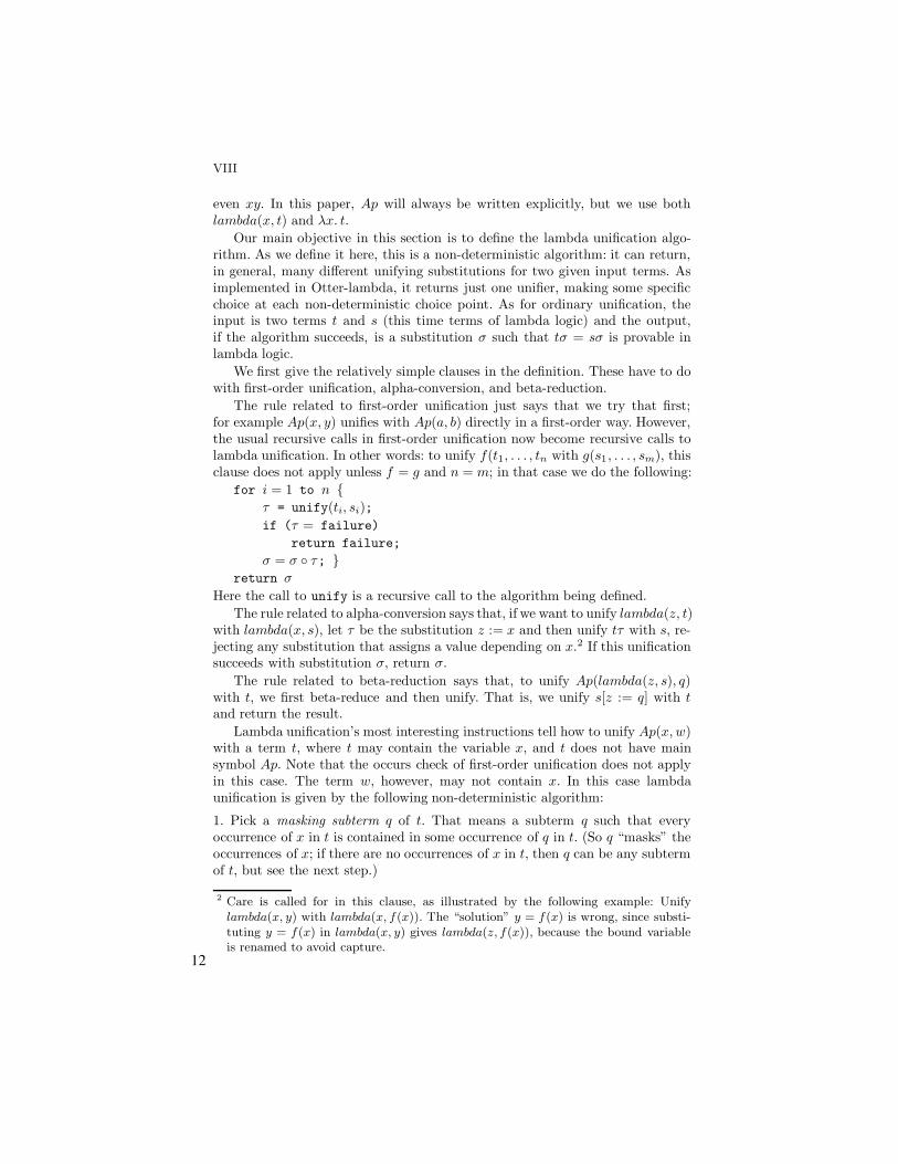
Lambda unification’s most interesting instructions tell how to unify Ap(x, w)with a term t, where t may contain the variable x, and t does not have mainsymbol Ap. Note that the occurs check of first-order unification does not applyin this case. The term w, however, may not contain x. In this case lambdaunification is given by the following non-deterministic algorithm:

1. Pick a masking subterm q of t. That means a subterm q such that everyoccurrence of x in t is contained in some occurrence of q in t. (So q “masks” theoccurrences of x; if there are no occurrences of x in t, then q can be any subtermof t, but see the next step.)

2 Care is called for in this clause, as illustrated by the following example: Unifylambda(x, y) with lambda(x, f(x)). The “solution” y = f(x) is wrong, since substi-tuting y = f(x) in lambda(x, y) gives lambda(z, f(x)), because the bound variableis renamed to avoid capture.

12

IX

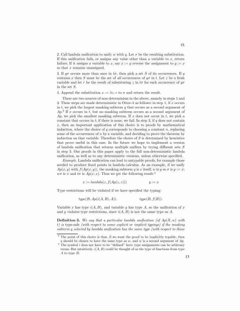
2. Call lambda unification to unify w with q. Let " be the resulting substitution.If this unification fails, or assigns any value other than a variable to x, returnfailure. If it assigns a variable to x, say x := y reverse the assignment to y := xso that x remains unassigned.3. If q" occurs more than once in t", then pick a set S of its occurrences. If qcontains x then S must be the set of all occurrences of q" in t. Let z be a freshvariable and let r be the result of substituting z in t" for each occurrence of q"in the set S.4. Append the substitution x := !z. r to " and return the result.

There are two sources of non-determinism in the above, namely in steps 1 and3. These steps are made deterministic in Otter-! as follows: in step 1, if x occursin t, we pick the largest masking subterm q that occurs as a second argument ofAp.3 If x occurs in t, but no masking subterm occurs as a second argument ofAp, we pick the smallest masking subterm. If x does not occur in t, we pick aconstant that occurs in t; if there is none, we fail. In step 3, if q does not containx, then an important application of this choice is to proofs by mathematicalinduction, where the choice of q corresponds to choosing a constant n, replacingsome of the occurrences of n by a variable, and deciding to prove the theorem byinduction on that variable. Therefore the choice of S is determined by heuristicsthat prove useful in this case. In the future we hope to implement a versionof lambda unification that returns multiple unifiers by trying di!erent sets Sin step 3. Our proofs in this paper apply to the full non-deterministic lambdaunification, as well as to any deterministic versions, unless otherwise specified.

Example. Lambda unification can lead to untypable proofs, for example thoseneeded to produce fixed points in lambda calculus. As an example, if we unifyAp(x, y) with f(Ap(x, y)), the masking subterm q is x itself; w is y so " is y := x;w" is x and t" is Ap(x, x). Thus we get the following result:4

x := lambda(z, f(Ap(z, z))) y := x

Type restrictions will be violated if we have specified the typing:

type(B, Ap(i(A, B), A)). type(B, f(B)).

Variable x has type i(A, B), and variable y has type A, so the unification of xand y violates type restrictions, since i(A, B) is not the same type as A.

Definition 3. We say that a particular lambda unification (of Ap(X, w) witht) is type-safe (with respect to some explicit or implicit typings) if the maskingsubterm q selected by lambda unification has the same type (with respect to those

3 The point of this choice is that, if we want the proof to be implicitly typable, thenq should be chosen to have the same type as w, and w is a second argument of Ap.

4 The symbol i does not have to be “defined” here; type assignments can be arbitraryterms. But intuitively, i(A,B) could be thought of as the type of functions from typeA to type B.

13

X

typings) as the term w, and q is a proper subterm of t (unless the two argu-ments of Ap have the same type). We also require that the value type assignedto Ap(X, w) is the same as the value type assigned to t.

The example preceding the definition illustrates a lambda unification that is nottype-safe for any reasonable typing. The masking subterm is x; type safety wouldrequire x to be assigned the same type as y. But x occurs as a first argumentof Ap and y as a second argument of Ap. Therefore the type specification of Apwould have to be of the form type(V, Ap(U, U )); but normally Ap will have atype specification of the form type(B, Ap(i(A, B), A)).

Remark. A discussion of the relationship, if any, between lambda unificationand the higher-type unification algorithms already in the literature is beyond thescope of this paper. The algorithms apply to di!erent systems and have di!erentdefinitions. Similarly, the exact relationship between lambda logic and varioussytems of higher-order logic, if there is any, is beyond the scope of this paper (orany paper of this length).

4 Implicit typing in lambda logic

If we consider the no-nilpotents example in lambda logic, we can state the axiomof mathematical induction in full generality, and Otter-lambda can use lambdaunification to find the specific instance of induction that is required. (See theexamples on the Otter-lambda website.) The proof, obtained without relativiz-ing to unary predicates, is correctly typable. This is not an accident: there aretheorems about implicit typing that guarantee it.

We first give an example to show that the situation is not as straightforwardas in first-order logic. If we use the axioms of group theory in lambda logic,must we relativize them to a unary predicate G(x)? As we have seen above,that is not necessary when doing first-order inference. We could, for example,put in some axioms about natural numbers, and not relativize them to a unarypredicate N (x), and as long as our axioms are correctly typed, our proofs willbe correctly typed too. There is, however, reason to worry about this when wemove to lambda logic.

In lambda calculus, every term has a fixed point. That is, for every term F wecan find a term q such that Ap(F, q) = q. Another form of the fixed point theoremsays that for each term H, we can find a term f such that Ap(f, x) = H(f, x).Applying this to the special case when H(f, x) = c ! Ap(f, x), where c is aconstant and ! is the group multiplication, we get Ap(f, x) = c ! Ap(f, x). Itfollows from the axioms of group theory that c is the group identity. On theother hand, in lambda logic it is given as an axiom that there exist two distinctobjects, say c and d, and since each of d and c must equal the group identity,this leads to a contradiction. Looked at model-theoretically, this means it isimpossible, given a lambda model M , to define a binary operation on M and anidentity element of M that make M into a group.

Since these axioms are contradictory in lambda logic, what is the value of aproof of a theorem from these axioms? One might think that there is none, and

14

XI

that to be able to trust an automatically produced proof from these axioms Iwould need to check it independently, or reformulate the axioms by relativizingthe group axioms to a unary predicate G. The point of this paper is that thereare good theoretical reasons why I do not need to do that. Even though thereexists a derivation of a contradiction in lambda logic from these axioms, it is nota well-typed derivation, and since the axioms are well-typed, the theorems inthis paper guarantee that deduced conclusions will also be well-typed. In otherwords, if we attempt to prove that every element is equal to c, we will put inthe negated goal x $= c, but if we use only “type-safe” lambda unification, asdefined below, we will not be able to construct the fixed point needed to derive acontradiction. If, however, we use unrestricted lambda unification, we can deriveit. If we put in the (negation of) the untyped fixed-point equation itself, thenwe can also prove that (even with type-safe lambda unification), but we need anon-well typed axiom in the input file.

First, let us consider how to type the relevant axioms. Writing G for the typeof group elements, 1 for the group identity, and i(G, G) for the type of maps fromG to G, we would have the following type specifications:

type(G, 1).type(G, !(G, G)).type(G, Ap(i(G, G), G).type(i(G, G), lambda(G, G)).

In general, of course, we want type(i(X, Y ), lambda(X, Y )), but the special caseshown is enough in this example. According to these type specifications, theaxioms are correctly typable, and when Otter-! produces a proof, the proofturns out to also be correctly typable. This is not an accident, as we will see.

In defining type specifications for lambda logic, the following technicalitycomes up: Normally in predicate logic we tacitly assume that di!erent symbolsare used for function symbols and predicate symbols. Thus P (P (c)) would not beconsidered a well-formed formula. In lambda logic we do wish to be able to definepropositional functions, as well as functions whose values are other objects, so weallow Ap both as a predicate symbol and a function symbol. However, except forAp, we follow the usual convention that predicate symbols and function symbolsuse distinct alphabets. This is the reason for clauses (4) and (5) in the followingdefinition.

Definition 4. A list of type specifications S is called coherent if(1) for each (predicate or function) symbol f ( except possibly Ap and lambda)and arity n, it contains at most one type specification of symbol f and arity n;the value type of a predicate symbol must be Prop and of a function symbol, mustnot be Prop.(2) type(i(X, Y ), lambda(X, Y )) belongs to S if and only if

type(Y, Ap(i(X, Y ), X)) belongs to S.(3) all type specifications with symbol Ap have the form type(V, Ap(i(U, V ), U )),for the same type U , which is called the “ground type” of S.

15

XII

(4) all type specifications with symbol lambda have the formtype(i(U, V ), lambda(U, V )),5 where U is the ground type of S.

(5) There are at most two type specifications in S with symbol Ap; if there aretwo, then exactly one must have value type Prop.

Conditions (2) and (3) guarantee that beta-reduction carries correctly typedterms to correctly typed terms. One might wish for a less restrictive condition in(4) and (5), allowing functions of functions, or functions of functions of functions,etc. But this is the condition for which we can prove theorems at the presenttime, and it covers a number of interesting examples in algebra and numbertheory.

If S is a coherent list S of type specifications, it makes sense to speak of “thetype assigned to a term t by S”, if there is at least one type specification in Sfor the main symbol and arity of t. Namely, unless the main symbol of t is Ap,only one specification in S can apply, and if the main symbol of t is Ap, then weapply the specification that does not have value type Prop. Similarly, it makessense to speak of “the type assigned to an atomic formula by S”. When the mainsymbol of t is Ap, we can speak of “the type assigned to t as a term” or “thetype assigned to t as a formula”, using the specification that does not or doeshave Prop for its value type.

Theorem 3. Let S be a coherent list of type specifications. Let s and t be twocorrectly typed terms or two correctly typed atomic formulas with respect to S.Let " be a substitution produced by successful type-safe lambda unification of sand t. Then s" and t" are correctly typed, and S assigns the same type to s, t,and s".

Example. Let s be Ap(X, w) and t be a+b. We can unify s and t by the substitu-tion " given by X := lambda(x, x + b) and w := a. If type(0, Ap(i(0, 0), 0)) andtype(0, +(0, 0)) then these are correctly typed terms and the types of s" and a+bare both 0. It may be that Ap also has a type specification type(Prop, Ap(i(0, P rop), 0)),used when the first argument of Ap defines a propositional function. However,this additional type specification will not lead to mis-typed unifications, sincethe two type specifications of Ap are coherent.Proof. We proceed by induction on the length of the computation by lambdaunification of the substitution ".

(i) Suppose s is a term f(r, q) (or with more arguments to f), and eitherf is not Ap, or r is neither a variable nor a lambda term. Then t also as theform f(R, Q) for some R and Q, and " is the result of unifying r with R toget r# = R# and then unifying q# with Q# , producing substitution $ so that" = # % $. By the induction hypothesis, r# is correctly typed and gets the sametype as r and R# ; again by the induction hypothesis, q#$ and Q#$ are correctlytyped and get the same type as q. Then s" = f(r", q") = f(r#$, q#$) is alsocorrectly typed.5 Intuitively, this says that if z has type X and t has type Y then lambda(z, t) has

type i(X,Y ), the type of functions from X to Y .16

XIII

(ii) The argument in (i) also applies if s is Ap(r, q) and t is Ap(R, Q) andlambda unification succeeds by unifying these terms as if they were first-orderterms.

(iii) If s is a constant then s" is s and there is nothing to prove.(iv) If s is a variable, what must be proved is that t and s have the same value

type. A variable must occur as an argument of some term (or atom) and hencethe situation really is that we are unifying P (s, . . .) with some term q, where Pis either a function symbol or a predicate symbol. If P is not Ap, then q musthave the form P (t, . . .), and t and s occur in corresponding argument positions(not necessarily the first as shown). Since these terms or atoms P (t, . . .) andP (s, . . .) are correctly typed, and S is coherent, t and s do have the same types.The case when P is Ap will be treated below.

(v) Suppose s is Ap(r, q), where r = lambda(z, p), and z does occur in p.Then s beta-reduces to p[z := q], and lambda unification is called recursively tounify p[z := q] with t. By induction hypothesis, t, t", p[z := q], and p[z := q]" arewell-typed and are assigned the same value type, which must be the value type,say V , of p. Since S is coherent, the type assigned to lambda(z, p) is i(U, V ),where U is the “ground type”, the type of the second arg of Ap. The type of q isU since q occurs as the second arg of Ap in the well-typed term s. The type ofs, which is Ap(r, q), is V . We must show that s" is well-typed and assigned thevalue type V . Now s" is Ap(r", q"). It su"ces to show that q" has type U andr" has type i(U, V ). We first show that the type of q" is U . Since z has typeU in lambda(z, p), q" occurs in the same argument positions in p[z := q]" as zdoes in p, and since z does occur at least once in p, and p[z := q]" is well-typed,q" must have the same type as z, namely U . Next we will show that r" hastype i(U, V ). We have r" = lambda(z, p)" = lambda(z, p") (since the boundvariable z is not in the domain of "). We have p"[z := q"] = p[z := q]"] and thetype of the latter term is V as shown above. The type of A[z := B] is the typeof A, and moreover A[z := B] is well-typed provided A and B are well-typedand z gets the same type as B. That observation applies here with A = p" andB = q", since the type of z is U and the type of q" is U . Therefore the typeof p" is the same as the type of p"[z := q"], which is the same as p[z := q]",which has type the same as p[z := q], which we showed above to be V . Sincer" = lambda(z, p"), and z has type U , r" has type i(U, V ), which was what hadto be proved.

(vi) There are two cases not yet treated: when s is Ap(X, w), and whens is a variable X occurring in the context Ap(X, w). We will treat these casessimultaneously. As described in the previous section, the algorithm will (1) selecta masking subterm q" of t" (2) unify w and q with result " (failing if this fails),(3) create a new variable z, and substitute z for some or all occurrences of q"in t", obtaining r, and (4) produce the unifying substitution " together withX := lambda(z, r).

Assume that t is a correctly typed term. Then every occurrence of q in thas the same type, by the definition of correctly typed. Since by hypothesisthis is type-safe lambda unification, q and w have the same type, call it U .

17

XIV

Since q unifies with w, by the induction hypothesis q" and w" are correctlytyped and get the same types as q and w, respectively, namely U . If Ap(X, w)has type Prop, then the type of s and that of t are the same by hypothesis.Otherwise, both occur as arguments of some function or predicate symbol P , incorresponding argument positions, and hence, by the coherence of S, they areassigned the same (value) type V . Then X has the type i(U, V ). We now assignthe fresh variable z the type U ; then r is also correctly typed, and gets the sametype V as s and t, since it is obtained by substituting z for some occurrencesof q" in t". For this last conclusion we need to use the fact that q is a propersubterm of t, by the definition of type-safe unification; hence r is not a variable,so the value type of r is well-defined, since S is coherent. Since S is coherent,there is a type specification in S of the form type(i(U, V ), lambda(U, V )). Thusthe term lambda(z, r) can be correctly typed with type i(U, V ), the same typeas X. Hence X" has the same type as X, and s" has the same type as s. Thatcompletes the proof of the theorem.

Theorem 4 (Implicit Typing for Lambda Logic). Let A be a set of clauses,and let S be a coherent set of type specifications such that each clause in Ais correctly typable with respect to S. Then all conclusions derived from A bybinary resolution, hyperresolution, factoring, paramodulation, and demodulation(including beta-reduction), using type-safe lambda unification in these rules ofinference, are correctly typable with respect to S, provided paramodulation from orinto variables are not allowed, and paramodulation into or from terms Ap(X, w)with X a variable is not allowed, and demodulators similarly are not allowed tohave variables or Ap(X, w) terms on the left.

Remark. The second restriction on paramodulation is necessary, as shown by thefollowing example. Suppose Ap has a type specification type(Prop, Ap(i, 0, P rop), 0)).Without the restriction, we could paramodulate from x + 0 = x into Ap(X, x),unifying x+0 with Ap(X, x) as in the example after Theorem 3, with the substi-tution X := lambda(x, x + 0). The conclusion of the paramodulation inferencewould be x. That is a mistyped conclusion, since x does not have the type Prop,although Ap does have value type Prop.Proof. Note that a typing assigns type symbols to variables, and the scope of avariable is the clause in which it occurs, so as usual with resolution, we assumethat all the variables are renamed, or indexed with clause numbers, or otherwisemade distinct, so that the same variable cannot occur in di!erent clauses. Inthat case the originally separate correct typings T [i] (each obtained from S byassigning values to varaibles in clause C[i]) can be combined (by union of theirgraphs) into a single typing T . We claim that the set of clauses A is correctlytyped with respect to this typing T . To prove this correctness we need to prove:

(i)each occurrence of a variable in A is assigned the same type by T . This fol-lows from the correctness of C[i], since because the variables have been renamed,all occurrences of any given variable are contained in a single clause C[i].

(ii) If r is f(u, v), and r occurs in A, and f(u, v),u, and v are assigned typesa,b,c respectively, then there is a type specification in S of the form type(a, f(b, c)).

18

XV

If the term r occurs in A, then r occurs in some C[i], so by the correctness ofT [i], there is a type specification in S as required.

(iii) each occurrence of each term r that occurs in A has the same value type.This follows from the coherence of S. The di!erent typings T [i] are not allowedto assign di!erent value types to the same symbol and arity.

Hence A is correctly typed with respect to T .All references to correct typing in the rest of the proof refer to the typing T .We prove by induction on the length of proofs that all proofs from A using

the specified rules of inference lead to correctly typed conclusions. The basecase of the induction is just the hypothesis that A is correctly typable. For theinduction step, we take the rules of inference one at a time. We begin with binaryresolution. Suppose the two clauses being resolved are P |Q and #R|B, wheresubstitution " is produced by lambda unification and satisfies P" = R". HereQ and B can stand for lists of more than one literal, in other words the rest ofthe literals in the clause, and the fact that we have shown P and #R as the firstliterals in the clause is for notational convenience only. By hypothesis, P |Q iscorrectly typed with respect to S, and so is #R|B, and by Theorem 3, P"|Q"and #R"|B" are also correctly typed. The result of the inference is Q"|B".But the union of correctly typed terms, literals, or sets of literals (with respectto a coherent set of type specifications) is again correctly typed, by the sameargument as in the first part of the proof. In other words, coherence implies thatif some subterm r occurs in both Q" and in B" then r gets the same valuetype in both occurrences. That completes the induction step when the rule ofinference is binary resolution.

Hyperresolution and negative hyperresolution can be “simulated” by a se-quence of binary resolutions, so the case in which the rule of inference is hyper-resolution or negative hyperresolution reduces to the case of binary resolution.The rule of “factoring” permits the derivation of a new clause by unifying twoliterals in the same clause that have the same sign, and applying the resultingsubstitution to the entire clause. By Theorem 3, a clause derived in this way iswell-typed if its premise is well-typed.

Now consider paramodulation. In that case we have already deduced t = qand P [z := r], and unification of t and r produces a substitution " such that t" =r". The conclusion of the rule is P [z := q"]. We have disallowed paramodulationfrom or into variables in the statement of the theorem; therefore t and r are notvariables. Let us write Type(t) for the value type of (any term) t. Because t = qis correctly typed, we have Type(t) = Type(q). If neither t nor q is an Ap term,then Type(t") = Type(q"), since they have the same functor. If one of themis an Ap term, then by hypothesis it is not of the form Ap(X, w), with X avariable. Then by Theorem 3, Type(t") = Type(t) and Type(q") = Type(q) =Type(t) = Type(t"). Thus in any case Type(q") = Type(t"). The value type ofr is the same at every occurrence, since P [z := r] is correctly typed. To showthat P [z := q"] is correctly typed, it su"ces to show that Type(q") = Type(r),which is the same as the type of r". Since the terms t and r unify, and neitheris a variable, their main symbols are the same, since by hypothesis r is not of

19

XVI

the form Ap(X, w). Hence Type(r) = Type(r") = Type(t") = Type(q"), whichis what had to be shown.

Now consider demodulation. In this case we have already deduced t = q andP [z := t"] and we conclude P [z := q"], where the substitution " is producedby lambda unification of t with some subterm $ of P [z := $]. Taking r = t", wesee that demodulation is a special case of paramodulation, so we have alreadyproved what is required. That completes the proof of the theorem.

Example: fixed points. The fixed point argument which shows that the groupaxioms are contradictory in lambda logic requires a term Ap(f, Ap(x, x)). Thepart of this that is problematic is Ap(x, x). If the type specification for Ap istype(V, Ap(i(U, V ), U )), then for Ap(x, x) to be correctly typed, we must haveV = U = i(U, U ). If U and V are type symbols, this can never happen, so thefixed point construction cannot be correctly typed. It follows from the theoremabove that this argument cannot be found by Otter-! from a correctly typedinput file. In particular, in lagrange3.in we have correctly typed axioms, so wewill not get a contradiction from a fixed point argument.

On the other hand, in file lambda4.in, we show that Otter-! can verify thefixed-point construction. The input file contains the negated goal

Ap(c, Ap(lambda(x, Ap(c, Ap(x, x))), lambda(x,Ap(c, Ap(x,x)))))$= Ap(lambda(x, Ap(c, Ap(x, x))), lambda(x, Ap(c,Ap(x, x)))).

Since this contains the term Ap(x, x), it cannot be correctly typed with respectto any coherent list of type specifications T . Otter-! does find a proof usingthis input file, which is consistent with our argument above that fixed-pointconstructions will not occur in proofs from correctly typable input files. The factthat the input file cannot be correctly typed, which we just observed directly,can also be seen as a corollary of the theorem, since Otter-! finds a proof. Thefact that the theoretical result agrees with the results of running the program isa good thing.

Remarks. (1) The (unrelativized) axioms of group theory are contradictoryin lambda logic, but if we put in only correctly-typed axioms, Otter-! will findonly correctly typed proofs, which will be valid in the finite type structure basedon any group, and hence will not be proofs of a contradiction.

(2) We already knew that resolution plus factoring plus paramodulation fromnon-variables is not refutation-complete, even for first-order logic; and we re-marked when pointing that out that this permits typed models of some theoriesthat are inconsistent when every object must have the same type. Here is anotherillustration of that phenomenon in the context of lambda logic.

(3) Of course Otter-lambda can find the fixed-point proof that gives thecontradiction; but to make it do so, we need to put in some non-well-typedaxiom, such as the negation of the fixed-point equation.

20

XVII

5 Enforcing type-safety

The theorems above are formulated in the abstract, rather than being theoremsabout a particular implementation of a particular theorem-prover. As a practicalmatter, we wish to formulate a theorem that does apply to Otter-! and coversthe examples posted on the Otter-! website, some of which have been mentionedhere. Otter-! never uses paramodulation into or from variables, so that hypoth-esis of the above theorems is always satisfied. But Otter-! does not always useonly type-safe lambda unification; nor would we want it to do so, since it can findsome untyped proofs of interest, e.g. fixed points, Russell’s paradox, etc. OnceOtter-! finds a correctly typable proof, we can check by hand (and could easilycheck by machine) that it is correctly typable. Nevertheless it is of interest to beable to set a flag in the input file that enforces type-safe unification. In Otter-!,if you put set(types) in the input file, then only certain lambda unificationswill be performed, and those unifications will always be type-safe.

Spefically, restricted lambda unification means that, when selecting a maskingsubterm, only a second argument of Ap or a constant will be chosen. This is therestriction imposed by the flag set(types). We now prove that this enforcestype safety under certain conditions.

Theorem 5 (Type safety of restricted lambda unification). Suppose thata given set of axioms admits a coherent type specification in which there is no typ-ing of the form Ap(U, U ), and all constants receive type U . Then all deductionsfrom the given axioms by binary resolution, factoring, hyperresolution, demodu-lation (including beta-reduction) paramodulation (except into or from variablesand Ap terms), lead to correctly typable conclusions, provided that restrictedlambda unification is used in those rules of inference.

Proof. It su"ces to show that lambda unifications will be type-safe under thesehypotheses. The unification of Ap(x, w) with t is type-safe (by definition) ifin step (1) of the definition of lambda unification, the masking subterm q oft has the same type as w. Now q is either a constant or term containing xthat appears as a second argument of Ap, since those are the “restrictions” inrestricted lambda unification. If q is a variable then it must be x, and mustoccur as a second argument of Ap; but x occurs as a first argument of Ap, andall second arguments of Ap get the same type, so there must be a typing ofthe form type(T, Ap(U, U )). But such a typing is not allowed, by hypothesis.Therefore q is not a variable. Then if q contains x, it must occur as a secondargument of Ap, as does w; hence by hypothesis w and q get the same type.Hence we may assume q is a constant. But by hypothesis, all constants get thesame type as the second arguments of Ap. That completes the proof.

6 Some examples covered by Theorem 5

It remains to substantiate the claims made in the abstract and introduction,that the theorems in this paper justify the use of implicit typing in Otter-! for

21

XVIII

the various examples mentioned. The first theorems apply in generality to anypartial implementation of non-deterministic lambda unification, used in com-bination with resolution and paramodulation, but disallowing paramodulationinto and from variables. Only Theorem 5 applies to Otter-lambda specifically,when the set(types) command is in the input file. We will now check explicitlythat interesting examples are covered by this theorem.

Let us start with the “no nilpotents” example. It appears prima facie not tomeet the hypotheses of Theorem 5, since that theorem requires that all constantshave the same type as the second argument of Ap. In this example the type of Apis the one needed for mathematical induction: type(Prop, Ap(i(N, Prop), N )), sothe type of the second arg of Ap is N ; but the axioms include a constant o forthe zero of the ring. This is not a serious problem: we can simply replace oin the axioms by zero(0), where zero is a new function symbol with the typespecification type(R, zero(N )). (The name zero is immaterial; this is just somefunction symbol.) The term zero(0) is not a constant, so it won’t be selected asa masking term (where it would interfere with the proof of Theorem 5). But itwill be treated essentially as a constant elsewhere in the inference process; and ifwe were worried about that, we could use a weight template to ensure that it hasthe same weight as a constant and hence will be treated exactly as a constant.On the logical side we have the following lemma to justify the claim:

Lemma 1. Let T be a theory with at least one constant c. Let T ! be obtainedfrom T by adding a new function symbol f , but no new axioms. Then (i) T ! plusthe axioms c = f(x) is conservative over T .

(ii) If T contains another constant b and we let Ao be the result of replacingc by f(b) in A, then T proves A if and only if T ! proves Ao.

(iii) There is an algorithm for transforming any proof of Ao in T ! to a proofof A in T .

Proof. (i) Every model of T can be expanded to a model of T ! plus c = f(x)by interpreting f as the constant function whose value is the interpretation of c.The completeness theorem then yields the stated conservative extension result.

(ii) Ao is equivalent to A in T ! plus c = f(x), so by (i), Ao is provable in T !

plus c = f(x) if and only if T proves A. In particular, if T ! proves Ao then Tproves A. Conversely, if T proves A and we just replace c with f(b) in the proof,we get a proof of Ao in T !.

(iii) The algorithm is fairly obvious: simply replace every term f(t) in theproof with c. (Not just terms f(b) but any term with functor f is replaced by c.)Terms that unify before this replacement will still unify after the replacement,so resolution proof steps will remain valid. The axioms of T ! plus c = f(x) areconverted to axioms of T plus c = c. Paramodulation steps remain paramod-ulation steps and demodulations remain demodulations. Since no variables areintroduced, paramodulations that were not from or into variables are still notfrom or into variables. That completes the proof of the lemma.

This lemma shows us that logically, the formulation of the no-nilpotents prob-lem with zero(0) for the ring zero is equivalent to the original formulation with

22

XIX

a constant o for the ring zero; and Theorem 5 directly applies to the formulationwith o(0). In practice, if we run Otter-lambda with o replaced by zero(0) inthe input file, we find the same proof as before, but with o replaced by zero(0).In essence this amounts to the observation that o was never used as a maskingterm in lambda unification in the original proof. Technically we should run theinput file with zero(0) first. Theorem 5 guarantees that if we find a proof, it willbe well-typed. The lemma guarantees that we can convert it into a proof of theoriginal formulation using a text editor to replace all terms with functor zeroby the original constant o.

Remark. Of course there is little di!erence between 0 and zero(0), and ofcourse we could allow the user of Otter-lambda to specify which constants have“ground type” and which do not, and only use constants of “ground type” inlambda-unification. In e!ect that is what this theorem allows us to do, withoutchecking the types of constants at run time: just rename all the “non-ground”constants by wrapping them in one extra function symbol.

We conclude with another example. Bernoulli’s inequality is

(1 + nx) < (1 + x)n if x > #1 and n > 0 is an integer.

Otter-lambda, in a version that calls on MathXpert [2] for “external simplifica-tion”, is able to prove this inequality by induction on n, being given only theclausal form of Peano’s induction axiom, with a variable for the induction pred-icate. The interest of the example in the present context is the fact that threetypes are involved: real numbers, positive integers, and propositions. The propo-sitional functions all have N , the non-negative integers, for the ground type, butthe types are not disjoint: N is a subset of the reals R. Moreover, the left-handside of the inequality uses n in multiplication, so if multiplication is typed totake two real arguments, the inequality as it stands will not be well-typed.

The solution is to introduce a symbol for an injection map i : N " R. Theinequality then becomes

(i(1) + i(n)x) < (i(1) + x)n

This formulation is well-typed, if we type i as a function from N to R. Again, inthe definition of exponentiation we have to use 0 for the natural number zero,and zero(0) for the real number zero, so that all the constants will have type N .If that is done, Theorem 5 applies, and we can be assured that the inference stepsperformed by Otter-lambda proper will lead from well-typed formulas to well-typed formulas. However, the theorem does not cover the external simplificationsteps performed by MathXpert. To ensure that these do not lead to mis-typedconclusions, we have to discard any results containing a minus sign or divisionsign, as that might lead out of the domain of integers. Problems involving em-bedded subtypes also arise even in typed theorem provers or proof checkers, soit is interesting that those problems are easily solved in lambda logic. The inter-ested reader can find the input and output files for this and other examples onthe Otter-lambda website.

23

XX

References

1. Beeson, M., Lambda Logic, in Basin, David; Rusinowitch, Michael (eds.) AutomatedReasoning: Second International Joint Conference, IJCAR 2004, Cork, Ireland, July4-8, 2004, Proceedings. Lecture Notes in Artificial Intelligence 3097, pp. 460-474,Springer (2004).

2. MathXpert Calculus Assistant, software available from (and described at)www.HelpWithMath.com.

3. McCune, W., Otter 3.0 Reference Manual and Guide, Argonne National LaboratoryTech. Report ANL-94/6, 1994.

4. Wick, C., and McCune, W., Automated reasoning about elementary point-set topol-ogy, J. Automated Reasoning 5(2) 239–255, 1989.

24

System Description: Leo – A Resolution based

Higher-Order Theorem Prover

Christoph Benzmuller

Fachbereich Informatik, Universitat des Saarlandes66041 Saarbrucken, Germany (www.ags.uni-sb.de/~chris)

Abstract. We present Leo, a resolution based theorem prover for clas-sical higher-order logic. It can be employed as both an fully automatedtheorem prover and an interactive theorem prover. Leo has been im-plemented as part of the !mega environment [23] and has been inte-grated with the !mega proof assistant. Higher-order resolution proofsdeveloped with Leo can be displayed and communicated to the user via!mega’s graphical user interface Loui. The Leo system has recentlybeen successfully coupled with a first-order resolution theorem prover(Bliksem).

1 Introduction

Many of today’s proof assistants such as Isabelle [22, 20], Pvs [21], Hol [12],Hol-Light [13], and Tps [2, 3] employ classical higher-order logic (also known asChurch’s simple type theory) as representation and reasoning framework. Oneimportant motivation for the development of automated higher-order proof toolsthus is to relieve the user of tedious interactions within these proof assistants byautomating less ambitious (sub)problems.

In this paper we present Leo, an automated resolution based theorem proverfor classical higher-order logic. Leo is based on extensional higher-order reso-lution which, extending Huet’s constrained resolution [14, 15], proposes a goaldirected, rule based solution for extensionality reasoning [6, 4, 5]. The main mo-tivation for Leo is to serve as an automated subsystem in the mathematicsassistance system !mega [23]. Additionally, Leo was intended to serve as astandalone automated higher-order resolution prover and to support the illus-tration and tutoring of extensional higher-order resolution. A previous systemdescription of Leo has been published in [7]. Novel in this system description isthe section on Leo’s interaction facilities and its graphical user interface. We alsoprovide more details on Leo’s automation and point to some recent extensions.

This system description is structured as follows: In Sections 2 and 3 we brieflyaddress Leo’s connection with !mega and Leo’s calculus. Section 4 presentsthe interactive theorem prover Leo and Section 5 the automated theorem proverLeo. In Section 6 we illustrate how Leo’s resolution proofs can be inspectedwith !mega’s graphical user interface Loui. Some experiments with Leo arementioned in Section 7 and Section 8 concludes the paper.

25

2 Leo is a Subsystem of !mega

Leo has been realized as a part of the !mega framework. This framework (andthus also Leo) is implemented in Clos [25], an object-oriented extension of Lisp.Leo is mainly dependent on !mega’s term datastructure package Keim. TheKeim package provides many useful data structures (e.g., higher-order terms,literals, clauses, and substitutions) and basic algorithms (e.g., application ofsubstitution, subterm replacement, copying, and renaming). Thus, the usageof Keim allows for a rather quick implementation of new higher or first-ordertheorem proving systems. In addition to the code provided by the Keim-package,Leo consists of approximately 7000 lines of Lisp code.

Amongst the benefits of the realization of Leo within the !mega frameworkare:

– Employing Keim supported a quick implementation of Leo. Important in-frastructure could be directly reused or had to be only slightly adapted orextended.

– An integration of Leo with the proof assistant and proof planner !mega

was easily possible.– Leo can easily be combined with other external systems already integrated

with !mega. Combinations of reasoning systems are particularly well sup-ported in !mega with the help of the agent based reasoning frameworkOants [8].

– Leo may retrieve and store theorems and definitions via !mega from Mbase,which is a structured repository of mathematical knowledge.

– Leo employs !mega’s input language Post.

There are also drawbacks of Leo’s realization as a part of !mega:

– Leo’s latest version is only available in combination with the !mega pack-age. Installation of !mega, however, is very complicated. Consequently,there is a conflict with the objective of providing a lean standalone theoremprover.

– The Keim datastructures are neither very e!cient nor are they optimizedor easily optimizable with respect to Leo.

!mega and with it Leo can be download from http://www.ags.uni-sb.de/˜omega.

3 Leo Implements Extensional Higher-Order Resolution

Leo is based on a calculus for extensional higher-order resolution. This calculusis described in [6, 4] and more recently in [5].

Extensionality treatment in this calculus is based on goal directed extension-ality rules which closely connect the overall refutation search with unificationby allowing for mutually recursive calls. This suitably extends the higher-orderE-unification and E-resolution idea, as it turns the unification mechanism intoa most general, dynamic theory unification mechanism. Unification may now

26

itself employ a Henkin complete higher-order theorem prover as a subordinatedreasoning system and the theory under consideration (which is defined by thesum of all clauses in the actual search space) dynamically changes.

In order to illustrate Leo’s extensional higher-order resolution approach wediscuss the TPTP (v3.0.1 as of 20 January 2005, see http://www.tptp.org) exam-ple SET171+3. This problem addresses distributivity of union over intersection1

!Ao!, Bo!, Co! A " (B # C) = (A " B) # (A " C)

In a higher-order context we can define the relevant set operations as follows

" := "Yo!, Zo! ("x! x $ Y % x $ Z)

# := "Yo!, Zo! ("x! x $ Y & x $ Z)

$:= "Z!, Xo! (X Z)

After recursively expanding the definitions in the input problem, i.e., com-pletely reducing it to first principles, Leo turns it into a negated unit clause. Un-like in standard first-order resolution, clause normalization is not a pre-processin Leo but part of the calculus. Internalized clause normalization is an impor-tant aspect of extensional higher-order resolution in order to support the (recur-sive) calls from higher-order unification to the higher-order reasoning process.Thus, Leo internally provides rules to deal with non-normal form clauses andthis is why it is su!cient to first turn the input problem into a single, usuallynon-normal, negated unit clause. Then Leo’s internalized clause normalizationprocess can take care of subsequent normalization.

In our concrete case, this normalization process leads to the following unitclause consisting of a (syntactically not solvable) unification constraint (hereBo!, Co!, Do! are Skolem constants and Bx is obtained from expansion of x $B):

[("x! Bx % (Cx & Dx)) =? ("x! (Bx % Cx) & (Bx % Dx))]

Note that negated primitive equations are generally automatically convertedby Leo into unification constraints. This is why [("x! Bx % (Cx & Dx)) =?

("x! (Bx % Cx) & (Bx % Dx))] is generated, and not [("x! Bx % (Cx & Dx)) =("x! (Bx%Cx)& (Bx%Dx))]F . Observe that we write [.]T and [.]F for positiveand negative literals, respectively. This unification constraint has no ’syntactic’pre-unifier. It is solvable ’semantically’ though with the help of the extensionality

1 We use Church’s notation o", which stands for the functional type " ! o. The readeris referred to [1] for a more detailed introduction. In the remainder, o will denote thetype of truth values and " defines the type of individuals. Other small Greek letterswill denote arbitrary types. Thus, Xo! (resp. its #-long form $y! Xy) is actually acharacteristic function denoting the set of elements of type % for which the predicateassociated with X holds. We use the square dot ‘ ’ as an abbreviation for a pair ofbrackets, where ‘ ’ stands for the left one with its partner as far to the right as isconsistent with the bracketing already present in the formula.

27

principles. Thus, Leo applies its goal directed functional and Boolean extension-ality rules which replace this unification constraint (in an intermediate step) bythe negative literal (where x is a Skolem constant):

[(Bx % (Cx & Dx)) ' ((Bx % Cx) & (Bx % Dx))]F

This intermediate unit clause is not in normal form and subsequent normalizationgenerates 12 clauses including the following four:

[Bx]F [Bx]T % [Cx]T [Bx]T % [Dx]T [Cx]F % [Dx]F

This set is essentially of propositional logic character and trivially refutable byLeo. For the complete proof of the problem Leo needs less than one second (ona notebook with an Intel Pentium M processor 1.60GHz and 2 MB cache) anda total of 36 clauses is generated.

4 Leo is an Interactive Theorem Prover

Leo is an interactive theorem prover based on extensional higher-order resolu-tion. The motivation for this is twofold. Firstly, the provided interaction featuressupport interaction with the automation of this calculus. For this an automatedproof attempt may be interrupted at any time and the system developer canthen employ the interaction facilities to investigate the proof state and to per-form some steps by hand. He may then again proceed with the automated proofsearch. Secondly, the interaction facilities can be employed for tutoring higher-order resolution in the classroom and they have in fact been employed for thispurpose.

We illustrate below an interactive session with Leo within the !mega sys-tem. For this we assume that the !mega system has already been started.Interaction within !mega is supported in two ways. We may use the graphicaluser interface Loui, or !mega’s older Emacs based command line interface.Both interfaces can be started and used simultaneously. In this section we de-scribe interaction only within the Emacs based interface. All commands couldalternatively also be invoked via Loui.

After starting !mega we are o"ered the following command line prompt inthe Emacs interface:

OMEGA:

We assume that we have added the following problem, formalized in Post,to !mega’s structured knowledge bass.

(Qo(o")(o") poo((ao"m") & ((bo"m") % (co"m"))) ) poo((ao"m") & (Qo(o")(o")co"bo"))

The Post representation of this problem is

28

(th~defproblem little(in base)(constants (p (o o)) (a (o i)) (b (o i)) (c (o i)) (m i))(conclusion(EXISTS (lam (Q (o (o i) (o i)))

(IMPLIES (p (AND (a m) (OR (b m) (c m))))(p (AND (a m) (Q c b))))))))

All problems have names and the name chosen for our problem is little. Thein-slot in this problem definition specifies Mbase theories from which furtherknowledge, e.g., definitions and lemmata, is inherited. Examples of some Mbase

theories are typed-set, relation, function, and group. Our very simpleexample problem is defined in the knowledge repository for theory base, and nofurther information is included. The assertion we want to prove is specified in theconclusion-slot and the typed constant symbols which occur in the assertionare declared in the constants-slot.

We now load all problems defined in theory base and then call the !mega

command show-problems to display the names of all problems. ’[...]’ indicatesthat some less interesting output information from Leo has been deleted herefor presentation purposes.

OMEGA: load-theory-problems base[...]

OMEGA: show-problems[...]EMBEDDEDlittleless-littleTEST[...]

Next we initialize the !mega proof assistant with the proof problem littleand display !mega’s central proof object after initialization.

OMEGA: prove littleChanging to proof plan LITTLE-1

OMEGA: show-pds...

LITTLE () ! (EXISTS [Q:(O (O I) (O I))] OPEN(IMPLIES(P (AND (A M) (OR (B M) (C M))))(P (AND (A M) (Q C B)))))

OMEGA:

Then we initialize Leo with this problem. Here we choose the default set-tings (suggested in the ’[]’-brackets) as input parameters for Leo. Each tactic(here EXT-INPUT-RECURSIVE) determines a specific flag setting of Leo. This flagsetting is displayed after initialization.

OMEGA: leo-initializeNODE (NDLINE) Node to prove with LEO: [LITTLE]TACTIC (STRING) The tactic to be used by LEO: [EXT-INPUT-RECURSIVE]THEORY-LIST (SYMBOL-LIST) Theories whose definitions will be expanded: [()]Expanding the Definitions....Initializing LEO....

29

Applying Clause Normalization....============== variable settings ================

Value(LEO*F-FO-ATP-RESOURCE) = 0Value(LEO*F-COOPERATE-WITH-FO-ATP) = NILValue(LEO*F-TACTIC) = EXT-INPUT-RECURSIVEValue(LEO*F-VERBOSE-HALF) = NILValue(LEO*F-VERBOSE) = NILValue(LEO*F-WEIGHT-AGE-INT) = 4Value(LEO*F-SOS-TYPE) = TOSETValue(LEO*F-USABLE-TYPE) = INDEXValue(LEO*F-CLAUSE-LENGTH-RESTRICTION) = NILValue(LEO*F-SAVE-FO-CLAUSES) = TValue(LEO*F-SUBSUM-MATCH-RESSOURCE) = NILValue(LEO*F-SOS-SUBSUMTION) = NILValue(LEO*F-BACKWARD-SUBSUMTION) = TValue(LEO*F-FORWARD-SUBSUMTION) = TValue(LEO*F-PARAMODULATION) = NILValue(LEO*F-REMOVE=EQUIV-NEG) = NILValue(LEO*F-REMOVE=EQUIV-POS) = NILValue(LEO*F-REMOVE=LEIBNIZ-NEG) = NILValue(LEO*F-REMOVE=LEIBNIZ-POS) = NILValue(LEO*F-EXT-DECOMPOSE-ONLY) = TValue(LEO*F-EXT-UNICONSTRCLS-ONLY) = NILValue(LEO*F-EXTENSIONALITY-NUM) = 6Value(LEO*F-EXT-INPUT-TREATMENT-RECURSIVE) = TValue(LEO*F-EXT-INPUT-TREATMENT) = NILValue(LEO*F-EXTENSIONALITY) = TValue(LEO*F-NO-FLEX-UNI) = NILValue(LEO*F-UNI-RESSOURCE) = 5Value(LEO*F-PRIM-SUBST-TYPES) = NILValue(LEO*F-PRIMITIVE-SUBSTITUTION) = TValue(LEO*F-FACTORIZE) = TValue(LEO*F-AUTO-PROOF) = NILValue(LEO*F-MAIN-COUNTER) = 0

=========== end variable settings =============

OMEGA:

During initialization Leo first recursively expands defined symbols occurringin the assumptions or the assertion with respect to the specified theories (herewe have none). Then it negates the assertion, turns it into a negated unit inputclause and subsequently normalizes it with its internalized normalization rules.The resulting clauses are put either into Leo’s set of support (if they stem fromthe assertion) or the usable set (if they stem from assumptions; here we havenone). Leo clauses have unique names starting with cl and followed by an au-tomatically created number. In ’( )’-brackets further clause specific informationfollows and the ’{ }’-brackets contain the clause literals. Negative literals havea leading - and positive literals a leading +. Type information is usually notdisplayed. All symbols starting with dc are free variables.

OMEGA: show-clauses================= BEGIN ===============================

The set of supportcl3(1.5|1):{(-(p (and (a m) (dc2 c b))))}cl4(1.5|1):{(+(p (and (a m) (or (b m) (c m)))))}

The set of usable clauses================= END =================================

Leo o"ers a list of commands, for instance, to apply calculus rules, to ma-nipulate and maintain the proof state, or to display information.

30

OMEGA: show-commands leo-interactive[...]DECOMPOSE: Applies decomposition on a clause.DELETE-CLAUSE: Deletes a clause from the current environment.END-REPORT: Closes the report stream.EXECUTE-LOG: Reads a log file stepwise and eventuelly stores

some of its commands in a new log file.EXIT: Leave the current command interpreter top level.EXT: Applies extensionality rule on a clause.[...]FACTORIZE: Applies factorization rule on a clause.[...]GUI-PROOF: Displays the LEO proof of node in the GUI.[...]LEO-PROVE: Prove with default parameter-settings.NEW-LOG: Sets the log mode and the log file name to the

given path name.PARA: Applies paramodulation rule on two clauses.PRE-UNIFIERS: Computes the pre-unifiers of a clause.PRE-UNIFY: Applies pre-unification on a clause.PRIM-SUBST: Applies primitive substitution rule on a clause.[...]READ-LEO-PROBLEM: Read a file, which contains a POST

representation of a problem, and transforms thisproblem into clause normal form.

[...]RESOLVE: Applies resolution rule on two clauses.SAVE-CLAUSE: Save a clause for use after termination of LEO

under its clausename.[...]SET-FLAG: Sets a global flagSET-TACTIC: Sets the tactic.SHOW-CLAUSE: Displays a clause, determined by name.SHOW-CLAUSES: Displays the two clause sets: the set of support

(LEO*G-SOS) and the set of usable clauses(LEO*G-USABLE).

[...]PROJECT: Applies projection rule on a clause.SHOW-DERIVATION: Displays a linearized derivation of a the clause.SHOW-FLAGS: Shows the global flagsSHOW-LEO-PROBLEM: Displays the given problem in POST.SHOW-LEO-PROOF: Displays the linearized LEO proofSHOW-TACTICS: Shows the tactics.SHOW-VARS: Shows the global vars.START-REPORT: Opens the tex and html report streams.STEP-LOG: Reads a log file stepwise and eventuelly stores

some of its commands in a new log file.SUBSUMES: Determines whether a clause subsumes another clause.[...]WRITE-DERIVATION: Writes the derivation of a clause in a file.WRITE-LOUIDERIVATION: Writes the derivation of a clause in LOUI format

in a file.WRITE-LOUIPROOF: Writes the proof in LOUI format in a file.WRITE-PROOF: Writes the proof in a file.

OMEGA:

We apply the resolution rule to the clause cl3 and cl4 on literal positions1 and 1 respectively. This results in the clause cl5 which consists only of aunification constraint. In this display unification constraints are presented asnegated equations (on the datastructure level they are distinguished from themas already mentioned in Section 3). Provided that we can solve the unificationconstraint cl5, we have found an empty clause and we are done.

OMEGA: resolve

31

NAME1 (STRING) of a clause: cl3NAME2 (STRING) of a clause: cl4POSITION1 (INTEGER) in clause 1: 1POSITION2 (INTEGER) in clause 2: 1Clause 1: cl3(1.5|1):{(-(p (and (a m) (dc2 c b))))}.Clause 2: cl4(1.5|1):{(+(p (and (a m) (or (b m) (c m)))))}.Res(CL3[1],CL4[1]):

(cl5(1|2):{(-(= (p (and (a m) (dc37 c b)))(p (and (a m) (or (b m) (c m))))))}).

OMEGA:

We ask Leo to compute the pre-unifiers for this unification constraint.

OMEGA: pre-unifiersNAME (STRING) of a clause: cl5The clause: cl5(1|2):{(-(= (p (and (a m) (dc37 c b)))

(p (and (a m) (or (b m) (c m))))))}.pre-unifiers: ({(dc37 --> [lam ?h45 ?h46.(or (?h46 m) (?h45 m))])}

{(dc37 --> [lam ?h45 ?h46.(or (?h46 m) (c m))])}{(dc37 --> [lam ?h45 ?h46.(or (b m) (?h45 m))])}{(dc37 --> [lam ?h45 ?h46.(or (b m) (c m))])}).

OMEGA:

Pre-unification of clause cl5 first generates these four pre-unifiers and thensubsequently applies them to cl5. Instantiation of di"erent pre-unifiers usuallyleads to di"erent result clauses. In our simple case here, however, we obtain fourcopies of the empty clause.

OMEGA: pre-unify cl5The clause: cl5(1|2):{(-(= (p (and (a m) (dc37 c b)))

(p (and (a m) (or (b m) (c m))))))}.Result: (cl14(0|3):{NIL} cl15(0|3):{NIL} cl16(0|3):{NIL} cl17(0|3):{NIL}).

OMEGA:

We now display the derivation of clause cl14 in the Emacs interface. cl14is the clause we obtain by application of the first pre-unifier from above. Theemployed pre-unifier (see clause cl7) is displayed in non-idempotent form. Afterapplying pre-unifiers Leo subsequently normalizes the resulting clauses. This iswhy we have this superfluous looking normalization step from cl7 to cl14.

OMEGA: show-derivation cl14================= clauses ===============================

Clause cl2 is #<Justified by ((Input))> :cl2(20|0):{(+(not (exists [lam dc-20735.(implies (p (and (a m) (or (b m) (c m))))

(p (and (a m) (dc-20735 c b))))])))}=============

================== proof ===================Clause cl2 is #<Justified by ((Input))> :cl2(20|0):{(+(not (exists [lam dc-20735.(implies (p (and (a m) (or (b m) (c m))))

(p (and (a m) (dc-20735 c b))))])))}=============

Clause cl3 is #<Justified by ((CNF)) on (cl2)> :cl3(1.5|1):{(-(p (and (a m) (dc-20738 c b))))}=============

Clause cl2 is #<Justified by ((Input))> :cl2(20|0):{(+(not (exists [lam dc-20735.

32

(implies (p (and (a m) (or (b m) (c m))))(p (and (a m) (dc-20735 c b))))])))}

=============Clause cl4 is #<Justified by ((CNF)) on (cl2)> :cl4(1.5|1):{(+(p (and (a m) (or (b m) (c m)))))}=============

Clause cl5 is #<Justified by((RES 1 1) (RENAMING {(dc2 --> dc37)})) on (cl3 cl4)> :cl5(1|2):{(-(= (p (and (a m) (dc37 c b)))

(p (and (a m) (or (b m) (c m))))))}=============

Clause cl7 is #<Justified by((UNI {(?h113 --> [lam ?h122 ?h123.m])

(?h107 --> [lam ?h120 ?h121.m])(?h101 --> [lam ?h111 ?h112.(?h111 (?h113 ?h111 ?h112))])(?h100 --> [lam ?h105 ?h106.(?h106 (?h107 ?h105 ?h106))])(dc37 --> [lam ?h98 ?h99.(or (?h100 ?h98 ?h99)

(?h101 ?h98 ?h99))])})(RENAMING {})) on (cl5)> :

cl7(0|2):{NIL}=============

Clause cl14 is #<Justified by ((CNF)) on (cl7)> :cl14(0|3):{NIL}=============

========== clauses in proof: 7 ============

OMEGA:

We now slightly modify our example problem and obtain a much harder one.

(Qo(o")(o") poo((ao"m") & ((bo"m") % (co"m"))) ) poo((Qo(o")(o")co"bo") & (ao"m"))

In Post this problem is represented as

(th~defproblem less-little(in base)(constants (p (o o)) (a (o i)) (b (o i)) (c (o i)) (m i))(conclusion(EXISTS (lam (Q (o (o i) (o i)))

(IMPLIES (p (AND (a m) (OR (b m) (c m))))(p (AND (Q c b) (a m))))))))

While problem little can still be solved by simple higher-order to first-ordertransformational approaches, this is not easily the case for the modified problemless-little since extensionality reasoning is required. The syntactic di"erenceto little, however, is small. We only switched the two inner conjuncts in theright hand side of the implication. We now first load the problem, then initializeLeo and then display Leo’s initial proof state.

OMEGA: prove less-littleChanging to proof plan LESS-LITTLE-1

OMEGA: show-pds...

LESS-LITTLE () ! (EXISTS [Q:(O (O I) (O I))] OPEN(IMPLIES(P (AND (A M) (OR (B M) (C M))))(P (AND (Q C B) (A M)))))

OMEGA: leo-initializeNODE (NDLINE) Node to prove with LEO: [LESS-LITTLE]TACTIC (STRING) The tactic to be used by LEO: [EXT-INPUT-RECURSIVE]

33

THEORY-LIST (SYMBOL-LIST) Theories whose definitions will be expanded: [()]Expanding the Definitions....[...]

OMEGA: show-clauses================= BEGIN ===============================

The set of supportcl3(1.5|1):{(-(p (and (dc-304 c b) (a m))))}cl4(1.5|1):{(+(p (and (a m) (or (b m) (c m)))))}

The set of usable clauses================= END =================================

OMEGA:

Again we resolve between clauses cl3 and cl4.

OMEGA: resolve cl3 cl4 1 1Clause 1: cl3(1.5|1):{(-(p (and (dc-304 c b) (a m))))}.Clause 2: cl4(1.5|1):{(+(p (and (a m) (or (b m) (c m)))))}.Res(CL3[1],CL4[1]): (cl5(1|2):{(-(= (p (and (dc1573 c b) (a m)))

(p (and (a m) (or (b m) (c m))))))}).

OMEGA:

Now the resulting clause cl5 is not pre-unifiable. Its unification constrainthas no ’syntactic’ solution.

OMEGA: pre-unifiers cl5The clause: cl5(1|2):{(-(= (p (and (dc1573 c b) (a m)))

(p (and (a m) (or (b m) (c m))))))}.pre-unifiers: NIL.

OMEGA: pre-unify cl5The clause: cl5(1|2):{(-(= (p (and (dc1573 c b) (a m)))

(p (and (a m) (or (b m) (c m))))))}.Result: NIL.

OMEGA:

However, there is a semantic solution which we find by application of Leo’scombined extensionality treatment. This first decomposes the unification con-straint and then applies Boolean extensionality (beforehand it usually tries toexhaustively apply functional extensionality, which is not applicable here).

OMEGA: decompose cl5The clause: cl5(1|2):{(-(= (p (and (dc1500 c b) (a m)))

(p (and (a m) (or (b m) (c m))))))}.Decomposed: (cl6(1|3):{(-(= (and (dc1500 c b) (a m))

(and (a m) (or (b m) (c m)))))}).

OMEGA: ext cl6The clause: cl6(1|3):{(-(= (and (dc1500 c b) (a m))

(and (a m) (or (b m) (c m)))))}Result: (cl14(4.5|4):{(+(a m) +(dc-4682 c b))}

cl13(6.0|4):{(+(c m) +(b m) +(dc-4681 c b))}cl12(1.5|4):{(+(a m))}cl11(4.5|4):{(+(c m) +(b m) +(a m))}cl10(6.0|4):{(-(b m) -(a m) -(dc-4680 c b))}cl9(6.0|4):{(-(c m) -(a m) -(dc-4679 c b))}).

OMEGA:

This set of resulting (first-order like) clauses is refutable and Leo can find arefutation. Unfortunately Leo is very bad at first-order reasoning (since it does

34

not employ optimizations and implementation tricks that are well known in thefirst-order community) and therefore the refutation of this clause set is not verye!cient. This motivates a cooperation with first-order provers; see Sections 5and 7 for further details.

5 Leo is an Automated Theorem Prover

Leo is first and foremost an automated theorem prover for classical higher-orderlogic. Within !mega it can be applied to prove (sub)problems automatically.Below we first reinitialize !mega with the problem less-little and then callLeo in its standard flag setting to it.

OMEGA: prove less-littleChanging to proof plan LESS-LITTLE-7

OMEGA: show-pds...

LESS-LITTLE () ! (EXISTS [Q:(O (O I) (O I))] OPEN(IMPLIES(P (AND (A M) (OR (B M) (C M))))(P (AND (Q C B) (A M)))))

OMEGA: call-leo-on-nodeNODE (NDLINE) Node to prove with LEO: [LESS-LITTLE]TACTIC (STRING) The tactic to be used by LEO: [EXT-INPUT-RECURSIVE]SUPPORTS (NDLINE-LIST) The support nodes: [()]TIME-BOUND (INTEGER) Time bound for proof attempt: [100]THEORY-LIST (SYMBOL-LIST) Theories whose definitions will beexpanded: [(ALL)]DEFS-LIST (SYMBOL-LIST) Symbols whose definitions will not beexpanded: [(= DEFINED EQUIV)]INSERT-FLAG (BOOLEAN) A flag indicating whether a partial result willbe automatically inserted.: [()]Looking for expandable definitions ....Initializing LEO....Applying Clause Normalization....[...]Start proving ...Loop: (100sec left)#1 (SOS 2 USABLE 0 EXT-QUEUE 0 FO-LIKE 4)

(99sec left)#2 (SOS 1 USABLE 1 EXT-QUEUE 0 FO-LIKE 4)

[...](94sec left)#29 (SOS 72 USABLE 12 EXT-QUEUE 0 FO-LIKE 98)

(91sec left)#30 (SOS 111 USABLE 13 EXT-QUEUE 0 FO-LIKE 138)

Total LEO time: 8446**** proof found (next clause nr: cl599) *****; cpu time (non-gc) 7,600 msec user, 0 msec system; cpu time (gc) 750 msec user, 10 msec system; cpu time (total) 8,350 msec user, 10 msec system; real time 8,451 msec; space allocation:; 8,909,213 cons cells, 3,568 symbols, 122,908,112 other bytes,; 0 static bytes

OMEGA:

35

Leo’s Architecture and Main Loop

Leo’s basic architecture adapts the set of support approach. The four corner-stones of Leo’s architecture (see Fig. 1) are:

EXT

Lightest

Resolved

Paramod

Prim!substFactorized

Ext!mod Uni!cont

USABLE

UnifiedProcessed

CONT

SOS1

2

45 6

7

9

9

9

11

13

123456789

10111213

choose lightest from SOSintegrate light. to USABLE

8

12

resolve with USABLEparamodulate with USABLEfactorize lightestprimitive substitution on lightest extensionality treatment on EXTpre!unification on CONT

store continuation objectcheck if extensionally interesting

3

10

implementednot yet implemented

integrate Unified into SOSpre!unification on Processed

Architecture of LEO

process results (tautology deletion)

Fig. 1. Leo’s main architecture (the ’dotted lines’ indicates functionalities which areusually disabled or not fully available yet)

USABLE The set of all usable clauses, which initially only contains clauses thatare assumed to be satisfiable, i.e., the clauses stemming from the assumptionsof the theorem to prove.

SOS The set of support, which initially only contains the clauses belonging tothe negated assertion.

EXT The set of all extensionally interesting clauses, i.e., heuristically determinedclauses which are stored for extensionality treatment. Initially this set isempty. See Step 12 of the main loop description below.

CONT The set of all continuations created by the higher-order pre-unificationalgorithm when reaching the pre-unification search depth limit. The idea isto support continuations of interrupted pre-unification attempts at a latertime. (This store is not activated yet in Leo)

36

Leo’s main loop (see Fig. 1) consists of the steps 1–13 as described below(the Initialize step is applied only at the very beginning of the proof attemptand is not part of the main loop). This loop, whose data-flow is graphicallyillustrated in Figure 1, is executed until an empty clause, i.e., a clause consistingno literals or only of flex-flex-unification constraints2, is detected.

Leo employs a higher-order subsumption test that is, apart from the tech-nical details, very similar to the ones employed in first-order provers. Instead offirst-order matching, the criteria for comparing the single literals is higher-ordersimplification matching, i.e., matching with respect to the deterministic higher-order simplification rules. It is theoretically possible to develop and employ amuch stronger subsumption filter in Leo. This is future work. However, a per-fect extensional higher-order subsumption filter, which would be the ideal case,is not feasible since extensional higher-order unification is undecidable.

Initialize The specified assumptions and the assertion are pre-clausified, i.e.,the assumptions become positive unit (pre-)clauses and the assertion be-comes a negative unit (pre-)clause. Definitions are expanded (with respectto the specified theories) and the pre-clauses are normalized. Within theclause normalization process the positive primitive equations are usually re-placed by respective Leibniz equations. Negative primitive equations are notexpanded but immediately encoded as extensional unification constraints.Furthermore, identical literals are automatically factorized. The assumptionclauses are passed to USABLE and the assertion clause to SOS.

Step 1 (Choose Lightest) Leo chooses the lightest (wrt. to a clause order-ing), i.e., topmost, clause from SOS. If this clause is a pre-clause, i.e., notin proper clause normal form, then Leo applies clause normalization to itand integrates the resulting proper clauses into SOS. Depending on the flag-setting forward and/or backward subsumption is applied; see also step 13).

Step 2 (Insert to USABLE) Leo inserts the lightest clause into USABLE whileemploying forward and/or backward subsumption depending on LEO’s over-all flag-setting.

Step 3 (Resolve) The lightest clause is resolved against all clauses in USABLEand the results are stored in RESOLVED.

Step 4 (Paramodulate) Paramodulation is applied between all clauses inUSABLE and the lightest clause, and the results are stored in PARAMOD. (Thisstep is currently not activated in Leo; currently Leibniz equality is globallyemployed instead of primitive equality.)

Step 5 (Factorize) The lightest clause is factorized and the resulting clausesare stored in FACTORIZED.

Step 6 (Primitive Substitution) Leo applies the primitive substitution prin-ciple to the lightest clause. The particular logical connectives to be imi-tated in this step are specified by a flag. The resulting clauses are stored inPRIM-SUBST.

2 A flex-flex-unification constraint has topmost free variables in each of the two termsto be unified. Flex-flex-constraints are always solvable.

37

Step 7 (Extensionality Treatment) The heuristically sorted store EXT con-tains extensionally interesting clauses (i.e., clauses with unification con-straints that may have additional pre-unifiers, if the extensionality rulesare taken into account). Leo chooses the topmost clause and applies thecompound extensionality treatment to all extensionally interesting literals.

Step 8 (Continue Unification) The heuristically sorted store CONT containscontinuations of interrupted higher-order pre-unification attempts from theprevious loops (cf. step 10). If the actual unification search depth limit (spec-ified by a flag, whose value can be dynamically increased during proof at-tempts) allows for a deeper search in the current loop, then the additionalsearch for unifiers will be performed. The resulting instantiated clauses arepassed to UNI-CONT and the new continuations are sorted and integratedinto CONT. (This step is currently not activated in Leo)

Step 9 (Collect Results) In this step Leo collects all clauses that have beengenerated within the current loop from the stores RESOLVED, PARAMOD,FACTORIZED, PRIM-SUBST, EXT-MOD, and UNI-CONT, eliminates obvious tau-tologies, and stores the remaining clauses in PROCESSED.

Step 10 (Pre-Unify) Leo tries to pre-unify the clauses in PROCESSED. Thus, itapplies the pre-unification rules exhaustively, thereby spanning a unificationtree until it reaches the unification search depth limit specified by a specialflag. The unification search depth limit specifies how many subsequent flex-rigid-branchings may at most occur in each path through the unificationsearch tree. The pre-unified, i.e., instantiated, clauses are passed to UNIFIED.The main idea of this step is to filter out all those clauses with syntacticallynon-solvable unification constraints (modulo the allowed search depth limit).But note that there are exceptions, which are determined in steps 11 and 12.That means that not all syntactically non-unifiable clauses are removed fromthe search space as this would, e.g., also remove the extensionally interestingclauses.

Step 11 (Store Continuations) Each time a pre-unification attempt in step10 is interrupted by reaching the unification search depth limit, a respectivecontinuation is created. This object stores the state of the interrupted uni-fication search process, i.e., it contains the particular unification constraintsas given at the point of interruption together with the remaining literals ofthe clause in focus and some information on the interrupted unification pro-cess. Continuations allow the prover to continue the interrupted unificationprocess at any later time. The set of all such continuations is integrated inthe sorted store CONT. (This step is not activated yet in Leo.)

Step 12 (Store Extensionally Interesting Clauses) In the pre-unificationprocess in step 10 Leo analyzes the unification pairs in focus in order toestimate whether this unification constraint and thus this clause is exten-sionally interesting, i.e., probably solvable with respect to both extensional-ity principles. All extensionally interesting clauses are passed to EXT, whichis heuristically sorted. While inserting the clauses into EXT forward and/orbackward subsumption is applied in order to minimize the number of clausesin this store.

38

Step 13 (Integrate to SOS) In the last step Leo integrates all pre-unifiedclauses in UNIFIED into the sorted store SOS. Forward and/or backward sub-sumption is employed depending on the flag-setting.

6 Visualizing Leo Derivations in Loui

!mega’s graphical user interface Loui [24] usually displays !mega proof ob-jects in multiple modalities: a graphical map of the proof tree, a linearized pre-sentation of the proof nodes with their formulae and justifications, and a termbrowser. Display of type information is optional and is determined by a switchin Loui.

Loui can be used to display proofs of other systems as well. Leo’s con-nection to Loui supports the graphical presentation of extensional higher-orderresolution derivations and proofs with the gain for the user that the structure ofinteractively or automatically created derivations becomes more transparent asis possible in the linearized display shown in Section 4.

Display of external proofs is supported by Loui via a specific interface lan-guage. In order to display Leo’s resolution proofs a simple mapping of the inter-nal proof state in Leo into this interface language is required. Fig. 2 illustratesthe Loui visualization of the automatically generated Leo proof for problemless-little from Section 5, and Fig. 3 displays part of the respective interfacelanguage representation of this proof.

7 Experiments with Leo

Leo has successfully been applied to di"erent higher-order examples. For ex-ample, in [4] Leo’s performance on simple examples about sets has been inves-tigated. One example is the already addressed TPTP problem SET171+3, i.e.,distributivity of union over intersection. Despite their simplicity such examplesare often non-trivial for automated first-order theorem provers. More details onthis discussion can be found in [9]. Further, proof examples have been investi-gated in [5].

In [9] a cooperation of Leo with a first-order theorem prover (we used the au-tomated theorem prover Bliksem [11] since this was already well integrated in theOMEGA framework) has been proposed and investigated. Thus, Leo has beenslightly extended so that it now constantly accumulates a bag of first-order likeclause. First-order like clauses do not contain any ‘real’ higher-order subterms(such as a "-abstraction or embedded equations), and are therefore suitable fortreatment by a first-order ATP or even a propositional logic decision procedureafter appropriate transformation. We use the transformation mapping as alsoemployed in Tramp [18], which has been previously shown to be sound and isbased on [17]. Essentially, it injectively maps expressions such as P (f(a)) to ex-pressions such as @1

pred(P, @1fun(f, a)), where the @ are new first-order operators

describing function and predicate application for particular types and arities.

39

Fig. 2. Loui usually displays !mega proof plans and !mega natural deduction proofs.In addition it can be employed to display Leo’s resolution proofs. Here we display thederivation of clause cl7 from example problem less-little.

40

[...]insertNode(grounded none "cl3" ["cl3""cl2"]"([NOT (O O)] ([P (O O)] ([AND (O O O)] ([DC-11438 (O (O I) (O I))]

[C (O I)] [B (O I)]) ([A (O I)] [M I]))))""((CNF))" ["cl2"] false)

insertNode(grounded none "cl4" ["cl4""cl2"]"([P (O O)] ([AND (O O O)] ([A (O I)] [M I]) ([OR (O O O)] ([B (O I)]

[M I]) ([C (O I)] [M I]))))""((CNF))" ["cl2"] false)

insertNode(grounded none "cl5" ["cl5""cl4""cl3""cl2"]"([NOT (O O)] ([= (O O O)] ([P (O O)] ([AND (O O O)] ([A (O I)] [M I])

([OR (O O O)] ([B (O I)] [M I]) ([C (O I)] [M I])))) ([P (O O)]([AND (O O O)] ([dc2762 (O (O I) (O I))] [C (O I)] [B (O I)])([A (O I)] [M I])))))"

"((RES 1 1) (RENAMING {(dc2705 --> dc2762)}))" ["cl4""cl3"] false)insertNode(grounded none "cl6" ["cl6""cl5""cl4""cl3""cl2"]"([NOT (O O)] ([= (O O O)] ([AND (O O O)] ([A (O I)] [M I]) ([OR (O O O)]

([B (O I)] [M I]) ([C (O I)] [M I]))) ([AND (O O O)] ([dc2762 (O (O I)(O I))] [C (O I)] [B (O I)]) ([A (O I)] [M I]))))"

"((DEC (1)))" ["cl5"] false)[...]

Fig. 3. Part of the Loui interface language representation of the Leo proof for problemless-little as communicated to Loui.

The injectivity of the mapping guarantees soundness, since it allows each proofstep to be mapped back from first-order to higher-order.

Whenever Leo creates a new clause it checks whether this is a first-orderlike clause, i.e., whether it is in the domain of the employed transformationalmapping. If this is the case, a copy of it is passed to the store of first-orderlike clauses. In each loop of Leo’s search procedure a fast first-order provercan now be applied to the set of first-order like clauses to find a refutation.In this case an overall proof has been found. The experiments in [9] show thatthis is a very promising approach to combining the benefits of higher-order andfirst-order theorem provers. Whereas this cooperative approach can solve theproblem less-little only slightly faster than Leo alone, many examples in [9]show that there are often significant improvements possible.

OMEGA: prove less-littleChanging to proof plan LESS-LITTLE-10

OMEGA: call-leo-on-nodeNODE (NDLINE) Node to prove with LEO: [LESS-LITTLE]TACTIC (STRING) The tactic to be usedby LEO: [EXT-INPUT-RECURSIVE]fo-atp-cooperationSUPPORTS (NDLINE-LIST) The support nodes: [()]TIME-BOUND (INTEGER) Time bound for proof attempt: [100]THEORY-LIST (SYMBOL-LIST) Theories whose definitions will beexpanded: [(ALL)]DEFS-LIST (SYMBOL-LIST) Symbols whose definitions will not beexpanded: [(= DEFINED EQUIV)]INSERT-FLAG (BOOLEAN) A flag indicating whether a partial resultwill be automatically inserted.: [()]Looking for expandable definitions ....Initializing LEO....Applying Clause Normalization....[...]

41

Start proving ...Loop: (100sec left)#1 (SOS 2 USABLE 0 EXT-QUEUE 0 FO-LIKE 4)

(99sec left)#2 (SOS 1 USABLE 1 EXT-QUEUE 0 FO-LIKE 4)

(98sec left)[...](96sec left)#9 (SOS 3 USABLE 4 EXT-QUEUE 0 FO-LIKE 12)

[...]Calling bliksem process 22267 with time resource 50sec .PARSING BLIKSEM OUTPUT ...Bliksem has found a saturation.

[...](96sec left)#10 (SOS 10 USABLE 5 EXT-QUEUE 0 FO-LIKE 20)

[...](94sec left)#21 (SOS 39 USABLE 9 EXT-QUEUE 0 FO-LIKE 60)Calling bliksem process 22454 with time resource 50sec .bliksem Time Resource in seconds:PARSING BLIKSEM OUTPUT ...Bliksem has found a proof.

Bliksem’s time:; cpu time (non-gc) 0 msec user, 0 msec system; cpu time (gc) 0 msec user, 0 msec system; cpu time (total) 0 msec user, 0 msec system; real time 174 msec; space allocation:; 416 cons cells, 0 symbols, 15,720 other bytes, 8936 static bytesInput Clauses: 75clauses generated: 37(94sec left)#22 (SOS 53 USABLE 10 EXT-QUEUE 0 FO-LIKE 75)

Total LEO time: 7262**** proof found (next clause nr: cl323) *****; cpu time (non-gc) 5,650 msec user, 20 msec system; cpu time (gc) 490 msec user, 0 msec system; cpu time (total) 6,140 msec user, 20 msec system; real time 7,273 msec; space allocation:; 5,218,155 cons cells, 1,886 symbols, 82,231,456 other bytes,; 49536 static bytes

8 Related Work and Conclusion

There are only very few automated theorem provers available for higher-orderlogic. Tps [2, 3], which is based on the mating search method, is the oldest andprobably still the strongest prover in this category. The extensionality reasoningof Tps has recently been significantly improved by Brown in his PhD thesis [10].

Related to the cooperation approach is the work of Hurd [16] which re-alizes a generic interface between higher-order logic and first-order theoremprovers. It is similar to the solution previously achieved by Tramp [18] in!mega. Both approaches pass essentially first-order clauses to first-order the-orem provers and then translate their results back into higher-order. More re-cent related work on the cooperation of Isabelle with the first-order theo-rem prover Vampire is presented in [19]. Further related work is Otter-" (seehttp://mh215a.cs.sjsu.edu/), which extends first-order logic with "-notation.

42

Leo has initially been implemented as a demonstrator system for extensionalhigher-order resolution in the context of the author’s PhD thesis [4]. The exper-iments carried out with Leo so far, in particular, its recent combination witha fast first-order theorem prover, have been very promising, and they motivatefurther work in this direction. This is particularly true since interactive proofassistants based on higher-order logic are recently gaining increasing attentionin formal methods.

During the implementation and later during the experiments many short-comings of Leo have been identified by the author. These shortcomings areboth of theoretical and of practical nature. Altogether this calls for a properreimplementation of Leo. This reimplementation should ideally be independentof !mega in order to provide a lean and easy to install and use automatedhigher-order theorem to the community.

References

1. P. Andrews. An Introduction to mathematical logic and Type Theory: To Truththrough Proof. Number 27 in Applied Logic Series. Kluwer, 2002.

2. P. B. Andrews, M. Bishop, and C. E. Brown. System description: TPS: A theoremproving system for type theory. In Conference on Automated Deduction, pages164–169, 2000.

3. P.B. Andrews, M. Bishop, S. Issar, D. Nesmith, F. Pfenning, and H. Xi. TPS: Atheorem proving system for classical type theory. Journal of Automated Reasoning,16(3):321–353, 1996.

4. C. Benzmuller. Equality and Extensionality in Higher-Order Theorem Proving.PhD thesis, Universitat des Saarlandes, Germany, 1999.

5. C. Benzmuller. Comparing approaches to resolution based higher-order theoremproving. Synthese, 133(1-2):203–235, 2002.

6. C. Benzmuller and M. Kohlhase. Extensional higher-order resolution. In Proc. ofCADE-15, number 1421 in LNAI. Springer, 1998.

7. C. Benzmuller and M. Kohlhase. LEO – a higher-order theorem prover. In Proc.of CADE-15, number 1421 in LNAI. Springer, 1998.

8. C. Benzmuller and V. Sorge. Oants – An open approach at combining Interactiveand Automated Theorem Proving. In Proc. of Calculemus-2000. AK Peters, 2001.

9. C. Benzmuller, V. Sorge, M. Jamnik, and M. Kerber. Can a higher-order anda first-order theorem prover cooperate? In F. Baader and A. Voronkov, editors,Proceedings of the 11th International Conference on Logic for Programming Arti-ficial Intelligence and Reasoning (LPAR), volume 3452 of LNAI, pages 415–431.Springer, 2005.

10. C. E. Brown. Set Comprehension in Church’s Type Theory. PhD thesis, Dept. ofMathematical Sciences, Carnegie Mellon University, USA, 2004.

11. H. de Nivelle. The Bliksem Theorem Prover, Version 1.12. Max-Planck-Institut,Saarbrucken, Germany, 1999. http://www.mpi-sb.mpg.de/˜bliksem/manual.ps.

12. M. Gordon and T. Melham. Introduction to HOL – A theorem proving environmentfor higher order logic. Cambridge University Press, 1993.

13. J. Harrison. The hol light theorem prover.14. G.P. Huet. Constrained Resolution: A Complete Method for Higher Order Logic.

PhD thesis, Case Western Reserve University, 1972.

43

15. G.P. Huet. A mechanization of type theory. In Donald E. Walker and Lewis Norton,editors, Proc. of the 3rd International Joint Conference on Artificial Intelligence(IJCAI73), pages 139–146, 1973.

16. J. Hurd. An LCF-style interface between HOL and first-order logic. In AutomatedDeduction — CADE-18, volume 2392 of LNAI, pages 134–138. Springer, 2002.

17. M. Kerber. On the Representation of Mathematical Concepts and their Translationinto First Order Logic. PhD thesis, Universitat Kaiserslautern, Germany, 1992.

18. A. Meier. TRAMP: Transformation of Machine-Found Proofs into Natural Deduc-tion Proofs at the Assertion Level. In Proc. of CADE-17, number 1831 in LNAI.Springer, 2000.

19. J. Meng and L. C. Paulson. Experiments on supporting interactive proof using res-olution. In Proc. of IJCAR 2004, volume 3097 of LNCS, pages 372–384. Springer,2004.

20. T. Nipkow, L.C. Paulson, and M. Wenzel. Isabelle/HOL: A Proof Assistant forHigher-Order Logic. Number 2283 in LNCS. Springer, 2002.

21. S. Owre, S. Rajan, J.M. Rushby, N. Shankar, and M. Srivas. PVS: Combiningspecification, proof checking, and model checking. In R. Alur and T. Henzinger,editors, Computer-Aided Verification, CAV ’96, number 1102 in LNCS, pages 411–414, New Brunswick, NJ, 1996. Springer.

22. L. Paulson. Isabelle: A Generic Theorem Prover. Number 828 in LNCS. Springer,1994.

23. J. Siekmann, C. Benzmuller, A. Fiedler, A. Meier, I. Normann, and M. Pollet.Proof development in OMEGA: The irrationality of square root of 2. In ThirtyFive Years of Automating Mathematics. Kluwer, 2003.

24. J. Siekmann, S. Hess, C. Benzmuller, L. Cheikhrouhou, A. Fiedler, H. Horacek,M. Kohlhase, K. Konrad, A. Meier, E. Melis, M. Pollet, and V. Sorge. LOUI:Lovely OMEGA user interface. Formal Aspects of Computing, 11:326–342, 1999.

25. G.L. Steele. Common Lisp: The Language, 2nd edition. Digital Press, Bedford,Massachusetts, 1990.

44

Combining Proofs of Higher-Order and

First-Order Automated Theorem Provers

Christoph Benzmuller1, Volker Sorge2, Mateja Jamnik3, and Manfred Kerber2

1Fachbereich Informatik, Universitat des Saarlandes66041 Saarbrucken, Germany (www.ags.uni-sb.de/~chris)2School of Computer Science, The University of Birmingham

Birmingham B15 2TT, England, UK (www.cs.bham.ac.uk/~vxs)3University of Cambridge Computer Laboratory

Cambridge CB3 0FD, England, UK (www.cl.cam.ac.uk/~mj201)

Abstract. !ants is an agent-oriented environment for combining infer-ence systems. A characteristics of the !ants approach is that a commonproof object is generated by the cooperating systems. This common proofobject can be inspected by verification tools to validate the correctnessof the proof. !ants makes use of a two layered blackboard architecture,in which the applicability of inference rules are checked on one (abstract)layer. The lower layer administrates explicit proof objects in a commonlanguage. In concrete proofs these proof objects can be quite bit, whichcan make communication during proof search very ine!cient. As a resultwe had situations in which most of the resources went into the overheadof constructing explicit proof objects and communicating between dif-ferent components. Therefore we have recently developed an alternativemodelling of cooperating systems in !ants which allows direct com-munication between related systems during proof search. This has theconsequence that proof objects can no longer be directly constructed andthus the correctness-validation in this novel approach is in question. Inthis paper we present a pragmatic approach how this can rectified.

1 Introduction

!ants is an agent-oriented environment for combining inference rules and in-ference systems. !ants was originally conceived to support interactive theoremproving but was later extended to a fully automated proving system [23, 8]. Acharacteristics of the !ants approach is that a joint proof object is generatedby the cooperating inference rules and inference systems. This joint proof objectcan be inspected by proof verification tools in combination with proof expansionin order to validate the correctness at a purely logic level. The !ants black-board architecture consists of two layers, an abstract upper layer, and a moredetailed lower layer. Applicability criteria for inference rules are modelled at theupper layer. The upper layer is supported by computations at the lower layerwhich models criteria for the instantiation of the parameters of the inferencerules.

45

External systems have been modelled in !ants as individual inference rulesat the upper layer. With this approach, !ants has been successfully employedin past experiments to check the validity of set equations using higher-orderand first-order theorem provers, model generation, and computer algebra [5].However, this approach was very ine!cient for hard examples because of thecommunication overhead imposed by the need to translate all steps into a com-mon proof data structure.

Therefore, we have recently developed an alternative approach: the single in-ference rule approach of cooperating systems in !ants which exploits the lowerlayer of the blackboard architecture. This approach has been successfully appliedto the combination of automated higher-order and first-order theorem provers.In particular, it has outperformed state-of-the-art first-order specialist reasoners(including Vampire 7.0) on 45 examples on sets, relations and functions; see [9].

Unfortunately, using a single inference rule approach, we had to sacrificethe generation of joint proof objects and correctness validation in this novelapproach. In this paper we present a pragmatic approach to how this can berectified.

The paper is structured as follows: In Section 2 we motivate and illustratethe cooperation between a higher-order theorem prover (we employ Leo [6]) anda first-order theorem prover (we employ Bliksem [12]). In Section 3 we comparethe two options for modelling cooperative reasoning systems in !ants: the initialmultiple inference approach and the novel single inference rule approach. InSection 4 we show how a joint proof object can also be obtained for the lattermodelling by mapping it back to the former. Section 5 concludes the paper.

2 Combining Higher-Order and First-Order ATP

2.1 Motivation

When dealing with problems containing higher-order concepts, such as sets, func-tions, or relations, today’s state-of-the-art first-order automated theorem provers(ATPs) still exhibit weaknesses on problems considered relatively simple by hu-mans (cf. [15]). One reason is that the problem formulations use an encodingin a first-order set theory, which makes it particularly challenging when tryingto prove theorems from first principles, that is, basic axioms. Therefore, to aidATPs in finding proofs, problems are often enriched by hand-picked additionallemmata, or axioms of the selected set theory are dropped leaving the theoryincomplete. This has recently motivated extensions of state-of-the-art first-ordercalculi and systems, as for example presented in [15] for the Saturate system.The extended Saturate system can solve some problems from the SET domainin the TPTP [25] which Vampire [22] and E-Setheo’s [24] cannot solve.

While it has already been shown in [6, 2] that many problems of this naturecan be easily proved from first principles using a concise higher-order represen-tation and the higher-order resolution ATP Leo [6], the combinatorial explosioninherent in Leo’s calculus prevents the prover from solving a whole range of

46

SET171+3 !Xo!, Yo!, Zo!.X " (Y # Z) = (X " Y ) # (X " Z)SET611+3 !Xo!, Yo!.(X # Y = $) % (X \ Y = X)SET624+3 !Xo!, Yo!, Zo!.Meets(X, Y # Z) % Meets(X, Y ) & Meets(X, Z)SET646+3 !x!, y" .Subrel(Pair(x, y), ("u!.') ( ("v" .'))SET670+3 !Zo!, Ro"!, Xo!, Yo".IsRelOn(R,X, Y ) )

IsRelOn(RestrictRDom(R, Z), Z, Y )

Table 1. Test Problems on Sets and Relations: Examples

possible problems with one universal strategy. Often higher-order problems re-quire only relatively few but essential steps of higher-order reasoning, while theoverwhelming part of the reasoning is first-order or even propositional level. Thissuggests that Leo’s performance could be improved when combining it with afirst-order ATP to search e!ciently for a possible refutation in the subset ofthose clauses that are essentially first-order.

The advantages of such a combination are not only that many problems canstill be e!ciently shown from first principles in a general purpose approach, butalso that problems can be expressed in a very concise way.

For instance, in [9] we present 45 problems from the SET domain of theTPTP-v3.0.1, together with their entire formalisation in less than two pages,which is di!cult to achieve within a framework that does not provide "-abstraction.We have used this problem set, which is an extension of the problems consideredin [15], to show the e"ectiveness of our approach (cf. [9]). While many of theconsidered problems can be proved by Leo alone with some strategy, the com-bination of Leo with the first-order ATP Bliksem [12] is not only able to solvemore problems, but also needs only a single strategy to prove them. Several ofour problems are considered very challenging by the first-order community andfive of them (of which Leo can solve four) have a TPTP rating of 1.00, sayingthat they cannot be solved by any TPTP prover to date.

Technically, the combination has been realised in the concurrent reasoningsystem !ants [23, 8] which enables the cooperation of hybrid reasoning systemsto construct a common proof object. In our past experiments, !ants has beensuccessfully employed to check the validity of set equations using higher-orderand first-order ATPs, model generation, and computer algebra [5]. While thisenabled a cooperation between Leo and a first-order ATP, the proposed solutioncould not be classified as a general purpose approach. A major shortcoming wasthat all communication of partial results had to be conducted via the commonproof object, which was very ine!cient for hard examples. Thus, the solved ex-amples from set theory were considered too trivial, albeit they were often similarto those still considered challenging in the TPTP in the first-order context.

In [9] we have presented our novel approach to the cooperation betweenLeo and Bliksem inside !ants by decentralising communication. As has beendocumented in [9] this leads not only to a higher overall e!ciency but also to ageneral purpose approach based on a single strategy in Leo.

47

2.2 Sets, Relations, and Functions: Higher-Order Logic Encoding

We list some examples of the test problems on sets and relations (and functions)that have been investigated in [9]. These test problems are taken from the TPTPagainst which we evaluated our system. The problems are given by the identi-fiers used in the SET domain of the TPTP, and are formalized in a variant ofChurch’s simply typed "-calculus with prefix polymorphism. In classical typetheory, terms and all their sub-terms are typed. Polymorphism allows the intro-duction of type variables such that statements can be made for all types. Forinstance, in problem SET171 in Table 1, the universally quantified variable Xo!

denotes a mapping from objects of type # to objects of type o. We use Church’snotation o#, which stands for the functional type # ! o. The reader is referredto [1] for a more detailed introduction. In the remainder, o will denote the typeof truth values, and small Greek letters will denote arbitrary types. Thus, Xo!

(and its $-longform "y! Xy) is actually a characteristic function denoting theset of elements of type #, for which the predicate associated with X holds. Asfurther notational convention, we use capital letter variables to denote sets, func-tions, or relations, while lower case letters denote individuals. Types are usuallyonly given in the first occurrence of a variable and omitted if inferable from thecontext. Table 1 presents some examples of the test problems investigated in [9].

These test problems employ defined concepts that are specified in a knowl-edge base of hierarchical theories that Leo has access to. Table 2 gives theconcepts necessary for defining the above problems:

!*

!:= "x!, Ao!.[Ax]

$ := ["x!.+]!#

!:= "Ao!, Bo!.["x!.x * A , x * B]

!"

!:= "Ao!, Bo!.["x!.x * A & x * B]

!\!

:= "Ao!, Bo!.["x!.x * A & x /* B]Meets(

!,!

) := "Ao!, Bo!.[-x!.x * A , x * B]Pair(

!,!

) := "x!, y" .["u!, v".u = x , v = y]!(

!:= "Ao!, Bo".["u!, v" .u * A , v * B]

Subrel(!

,!

) := "Ro"!, Qo"!.[!x!, y".Rxy ) Qxy]IsRelOn(

!,!

,!

) := "Ro"!, Ao!, Bo".[!x!, y" .Rxy ) x * A , y * B]RestrictRDom(

!,!

) := "Ro"!, Ao!.["x!, y" .x * A , Rxy]

Table 2. Definitions of Operations on Sets and Relations: Examples

These concepts are defined in terms of "-expressions and they may containother, already specified concepts. For presentation purposes, we use customarymathematical symbols ",#, etc., for some concepts like union, intersection, etc.,and we also use infix notation. For instance, the definition of union on sets inTable 2 can be easily read in its more common mathematical representationA"B := {x|x $ A% x $ B}. Before proving a problem, Leo always expands —

48

Assumptions: !B, C, x [x * (B " C) % x * B & x * C] (1)

!B, C, x [x * (B # C) % x * B , x * C] (2)

!B, C [B = C % B . C , C . B] (3)

!B, C [B " C = C " B] (4)

!B, C [B # C = C # B] (5)

!B, C [B . C % !x x * B ) x * C] (6)

!B, C [B = C % !x x * B % x * C] (7)

Proof Goal: !B, C, D [B " (C # D) = (B " C) # (B " D)] (8)

Table 3. Problem SET171+3: The First-Order TPTP Encoding.

recursively, if necessary — all occurring concepts. This straightforward expansionto first principles is realised by an automated preprocess in our current approach.

2.3 Sets, Relations, and Functions: First-Order Logic Encoding

Let us consider example SET171+3 in its first-order formulation from the TPTP(see Table 3). We can observe that the assumptions provide only a partial ax-iomatisation of naive set theory. On the other hand, the specification introduceslemmata that are useful for solving the problem. In particular, assumption (7) istrivially derivable from (3) with (6). Obviously, clausal normalisation of this first-order problem description yields a much larger and more di!cult set of clauses.Furthermore, definitions of concepts are not directly expanded as in Leo. Itis therefore not surprising that most first-order ATPs still fail to prove thisproblem. In fact, very few TPTP provers were successful in proving SET171+3.Amongst them are Muscadet 2.4. [21], Vampire 7.0, and Saturate. The nat-ural deduction system Muscadet uses special inference rules for sets and needs0.2 seconds to prove this problem. Vampire needs 108 seconds. The Saturate

system [15] (which extends Vampire with Boolean extensionality rules thatare a one-to-one correspondence to Leo’s rules for Extensional Higher-OrderParamodulation [3]) can solve the problem in 2.9 seconds while generating 159clauses. The significance of such comparisons is clearly limited since di"erentsystems are optimised to a di"erent degree. One noted di"erence between theexperiments with first-order provers listed above, and the experiments with Leo

and Leo-Bliksem is that first-order systems often use a case tailored problemrepresentation (e.g., by avoiding some base axioms of the addressed theory),while Leo and Leo-Bliksem have a harder task of dealing with a general (notspecifically tailored) representation. Thus, the comparison of the performanceof Leo and Leo-Bliksem with first-order systems as done in [9] is unfair: thehigher-order systems attack harder, non-tailored problems. Nevertheless, as wedemonstrated by the performance results in [9] the higher-order systems stillperform better.

49

(1) !B,C, D.B " (C # D) = (B " C) # (B " D)/ clause initialization/ def.-expansion, cnf/ B, C, D Skolem const.

(2) [("x.Bx & (Cx , Dx))= ("x.(Bx , Cx) & (Cx , Dx))]F

/ unification constraint(3) [("x.Bx & (Cx , Dx))=?("x.(Bx , Cx) & (Cx , Dx))]

/ f-extensionality/ x new Skolem constant

(4) [(Bx & (Cx , Dx))=?((Bx , Cx) & (Cx , Dx))]/ B-extensionality

(5) [(Bx & (Cx , Dx))%((Bx , Cx) & (Cx , Dx))]F

/ cnf, factor., subsumption(6) [Bx]F

(7) [Bx]T&[Cx]T propositional problem!(8) [Bx]T&[Dx]T

(9) [Cx]F&[Dx]F

/ propositional reasoning(10) !

Table 4. Problem SET171+3: Solution in Leo

For the experiments with Leo and the cooperation of Leo with the first-ordertheorem prover Bliksem, "-abstraction as well as the extensionality treatmentinherent in Leo’s calculus [4] is used. This enables a theoretically1 Henkin-complete proof system for set theory. In the above example SET171+3, Leo gen-erally uses the application of functional extensionality to push extensional unifi-cation constraints down to base type level, and then eventually applies Booleanextensionality to generate clauses from them. These are typically much simplerand often even propositional-like or first-order-like (FO-like, for short), that is,they do not contain any ‘real’ higher-order subterms (such as a "-abstraction orembedded equations), and are therefore suitable for treatment by a first-orderATP or even a propositional logic decision procedure.

2.4 Solving the Test Problem SET171+3 in Leo

Table 4 illustrates how Leo tackles and solves the test problem SET171+3. Firstthe resolution process is initialised, that is, the definitions occurring in the inputproblem are expanded, that is, completely reduced to first principles. Then theproblem is turned into a negated unit clause. The resulting (not displayed inter-mediate) clause is not in normal form and therefore Leo first normalizes it withexplicit clause normalisation rules (cnf) to reach some proper initial clauses. In

1 For pragmatic reasons, such as e!ciency, most of Leo’s tactics are incomplete. Leo’sphilosophy is to rely on a theoretically complete calculus, but to practically providea set of complimentary strategies so that these cover a broad range of theorems.

50

our concrete case, this leads to the unit clause (2). Note that negated prim-itive equations are generally automatically converted by Leo into unificationconstraints. This is why (2) is automatically converted into (3), which is a syn-tactically not solvable, but is a semantic unification problem. Observe, that wewrite [.]T and [.]F for positive and negative literals, respectively. Leo then appliesits goal directed functional and Boolean extensionality rules which replace theunification constraint (3) by the clauses (4) and (5). Unit clause (5) is again notnormal; normalisation, factorisation and subsumption yields the clauses (6)-(9).This set is essentially of propositional logic character and trivially refutable. Leo

needs 0.56 seconds for solving the problem and generates a total of 36 clauses.

2.5 Solving the Test Problem SET171+3 in Leo-Bliksem

As illustrated in Table 4, Leo transforms test problem SET171+3 straight-forwardly into a propositional like subproblem. Here the generated clause set(7)–(10) can still be e!ciently refuted by Leo. Generally, however, the gener-ated subsets of propositional or first-order like subproblems may quickly becomeso big that Leo’s refutation procedure, which is not optimised for these prob-lem classes, gets stuck. And in Leo’s search space generally some further realhigher-order clauses have to be taken into account. This observation motivatesour cooperative Leo-Bliksem proof search approach: while Leo performs itsproof search as before, it periodically also passes the detected first-order likeclauses (which, of course, include the propositional like clauses) to the first-orderspecialist reasoner Bliksem. We note:

– The generated first-order like clauses in Leo are copied into a special bagwhich never decreases and usually always increases. That is, the bag of first-order like clauses dynamically changes and eventually becomes refutable(such as clauses (7)–(10) in our example).

– Leo’s proof search procedure remains unchanged and Leo still tries to refutesuch subproblems itself (as before) in a bigger context.

– In addition, specialist reasoners may now support Leo by showing that thebag of first-order like subproblems is refutable.

– Each time the bag of first-order like subproblems is increased by Leo, a newinstance of a specialist reasoner is launched (with a resource-bound). Thisinstance runs in parallel to Leo’s proof search and may eventually signalsuccess to Leo. If Leo receives such a success signal, it stops its own proofsearch and reports that a cooperative proof has been found. Alternatively(as before) Leo stops proof search when it finds the proof itself.

– Our cooperative approach can easily be fine-grained by separating the bag offirst-order like clauses into even more specialised subclasses, such as propo-sitional logic, guarded fragment, etc. Di"erent specialist reasoners can thenbe employed to attack these clause sets.

– For the higher-order problems investigated in [9] we further observe:• Some problems are immediately mapped by recursive definition expan-

sion (without extensionality reasoning) and normalisation into first-orderlike problems; an example is SET624+3.

51

• Some problems are immediately mapped by recursive definition expan-sion (without extensionality reasoning) and normalisation into the emptyclause such that proof search does not even start; an example is SET646+3.

• Some problems require several rounds of extensionality processing withinLeo’s set-of-support based proof search procedure before the bag of first-order like clauses turns into a refutable set of clauses; an example isSET611+3.

The result of the case study performed in [9] is: The Leo-Bliksem cooper-ation impressively outperforms both state-of-the art first-order specialists (in-cluding Vampire 7.0) and the non-cooperative Leo system.

In the next section we describe in more detail how the cooperative proofsearch approach between Leo and the first-order prover Bliksem has been mod-elled in !ants.

3 !ants

!ants was originally conceived to support interactive theorem proving but waslater extended to a fully automated proving system [23, 8]. Its basic idea is tocompose a central proof object by generating, in each proof situation, a rankedlist of potentially applicable inference steps. In this process, all inference rules,such as calculus rules or tactics, are uniformly viewed with respect to threesets: premises, conclusions, and additional parameters. The elements of thesethree sets are called arguments of the inference rule and they usually dependon each other. An inference rule is applicable if at least some of its argumentscan be instantiated with respect to the given proof context. The task of the!ants architecture is now to determine the applicability of inference rules bycomputing instantiations for their arguments.

The architecture consists of two layers. On the lower layer, possible instanti-ations of the arguments of individual inference rules are computed. In particular,each inference rule is associated with its own blackboard and concurrent pro-cesses, one for each argument of the inference rule. The role of every process isto compute possible instantiations for its designated argument of the inferencerule, and to record these on the blackboard. The computations are carried outwith respect to the given proof context and by exploiting information alreadypresent on the blackboard, that is, argument instantiations computed by otherprocesses. On the upper layer, the information from the lower layer is used forcomputing and heuristically ranking the inference rules that are applicable inthe current proof state. The most promising rule is then applied to the centralproof object and the data on the blackboards is cleared for the next round ofcomputations.

!ants employs resource reasoning to guide search.2 This enables the con-trolled integration (e.g., by specifying time-outs) of full-fledged external reason-

2 !ants provides facilities to define and modify the processes at run-time. But noticethat we do not use these advanced features in the case study presented in this paper.

52

ing systems such as automated theorem provers, computer algebra systems, ormodel generators into the architecture.

3.1 Cooperation via multiple inference rules

The use of the external systems is modelled by inference rules, usually one foreach system. Their corresponding computations are encapsulated in one of theindependent processes in the architecture. For example, an inference rule mod-elling the standard application Leo has its conclusion argument set to be anopen higher-order (HO) goal.

HO-goalLeo (LEO-parameters)

A process can then place an open goal on the blackboard, where it is pickedup by a process that applies the Leo prover to it. Any computed proof from theexternal system is again written to the blackboard from where it is subsequentlyinserted into the proof object when the inference rule is applied. While this setupenables proof construction by a collaborative e"ort of diverse reasoning systems,the cooperation can only be achieved via the central proof object. This meansthat all partial results have to be translated back and forth between the syntaxesof the integrated systems and the language of the proof object. For modellingthe cooperation of Leo with a first-order reasoner we have first experimentedwith the following multiple inference rule modelling (see also [5]):

Neg-Conj-of-FO-clauses

HO-goalLeo-with-partial-result(Leo-parameters)

FO-goalBliksem (Bliksem-parameters)

The first rule models a process that picks up higher-order proof problem fromthe blackboard, passes it to Leo which starts its proof search, and then returnsthe negated conjunction of generated first-order clauses back (e.g. the negatedconjunction of the clauses (7)–(10) in our previous example). For each modifiedbag of first-order like clauses in Leo this rule may suggest a novel reduction ofthe original higher-order goal to a first-order criterion.

Since there are many types of integrated systems, the language of the proofobject maintained in !ants — a higher-order language even richer than Leo’s,together with a natural deduction calculus — is expressive but also cumbersome.This leads not only to a large communication overhead, but also means thatcomplex proof objects have to be created, even if the reasoning of all systemsinvolved is clause-based. Large clause sets need to be transformed into largesingle formulae to represent them in the proof object; the support for this in!ants to date is ine!cient. Consequently, the cooperation between externalsystems is typically rather ine!cient [5].

53

3.2 Cooperation via a single inference rule

In order to overcome the problem of the communication bottleneck describedabove, we devised a new method for the cooperation between a higher-orderand a first-order theorem prover within !ants. Rather than modelling eachtheorem prover as a separate inference rule (and hence needing to translatethe communication via the language of the central proof object), we model thecooperation between a higher-order (concretely, Leo) and a first-order theoremprover (in our case study Bliksem) in !ants as a single inference rule.

HO-goalLeo-Bliksem (

Leo-partial-proof, FO-clauses, FO-proof, Leo-parameters, Bliksem-parameters

)

The communication between the two theorem provers is carried out directlyby the parameters of the inference rule and not via the central proof object. Thisavoids translating clause sets into single formulae and back.

Concretely, the single inference rule modelling the cooperation between Leo

and a first-order theorem prover needs the following arguments to be applicable:(1) an open higher-order proof goal, (2) a partial Leo proof, (3) a set of FO-like clauses in the partial proof, (4) a first-order refutation proof for the setof FO-like clauses, and (5) and (6) the usual flag-parameters for the theoremprovers Leo and Bliksem. Each of these arguments is computed, that is, itsinstantiation is found, by an independent process. The first process finds opengoals in the central proof object and posts them on the blackboard associatedwith the new rule. The second process starts an instance of the Leo theoremprover for each new open goal on the blackboard. Each Leo instance maintainsits own set of FO-like clauses. The third process monitors these clauses, and assoon as it detects a change in this set, that is, if new FO-like clauses are added byLeo, it writes the entire set of clauses to the blackboard. Once FO-like clausesare posted, the fourth process first translates each of the clauses directly intoa corresponding one in the format of the first-order theorem prover, and thenstarts the first-order theorem prover on them. Note that writing FO-like clauseson the blackboard is by far not as time consuming as generating higher-orderproof objects. As soon as either Leo or the first-order prover finds a refutation,the second process reports Leo’s proof or partial proof to the blackboard, thatis, it instantiates argument (2). Once all four arguments of our inference ruleare instantiated, the rule becomes applicable and its application closes the openproof goal in the central proof object. That is, the open goal is proved by thecooperation between Leo and a first-order theorem prover. When computingapplicability of the inference rule, the second and the fourth process concurrentlyspawn processes running Leo or a first-order prover on a di"erent set of FO-likeclauses. Thus, when actually applying the inference rule, all these instances ofprovers working on the same open subgoal are stopped.

While in the previous approach with multiple inference rules the cooperationbetween Leo and Bliksem was modelled at the upper layer of the !ants ar-chitecture, our new approach models their cooperation by exploiting the lower

54

layer of the !ants blackboard architecture. This is not an ad hoc solution,but rather, it demonstrates !ants’s flexibility in modelling the integration ofcooperative reasoning systems.

Our approach to the cooperation between a higher-order and a first-ordertheorem prover has many advantages. The main one is that the communicationis restricted to the transmission of clauses, and thus it avoids any intermediatetranslation into the language of the central proof object. This significantly re-duces the communication overhead and makes e"ective proving of more involvedtheorems feasible.

4 Constructing a Combined Proof Object

A disadvantage of our approach is that we cannot easily translate and integratethe two proof objects produced by Leo and Bliksem into the central proof ob-ject maintained by !ants. This has been possible in our previous approach withmultiple inference rules. Thus, we developed a simple and pragmatic solution tothe problem:

– The main idea is to replay the proof on the upper level of the !ants archi-tecture (using the multiple inference rule modelling) once a proof attemptwas successful (with a single inference rule modelling) on the lower level.

– We can essentially reconstruct all the information from the blackboard thatwe need in order to replay the proof. For this remember that the rule Leo-Bliksem is only applicable if all parameters of the rule are instantiated,that is, the respective parameter instantiation information is available onthe blackboard for each successful cooperative proof attempt. Respectiveinstantiation information generated from a successful cooperative proof at-tempt for our running example SET171+3, for instance, is:

HO-Goal := &B, C, D.C " (B # D) = (C " B) # (C " D)

Leo-partial-proof := . . . a HO resolution proof object % . . .

FO-clauses := (7) [Bx]F

(8) [Bx]T%[Cx]T

(9) [Bx]T%[Dx]T

(10) [Cx]F%[Dx]F

FO-proof := . . . a FO resolution proof object & . . .

Leo-parameters := . . . the flags chosen for the Leo call . . .

Bliksem-parameters := . . . the flags chosen for the Bliksem call . . .

– For finding joint proofs e!ciently in our experiment we called Bliksem inthe fastest mode. In this case the generated FO-proof object is typically verysparse, i.e. contains only very little information for proof reconstruction andtransformation.

55

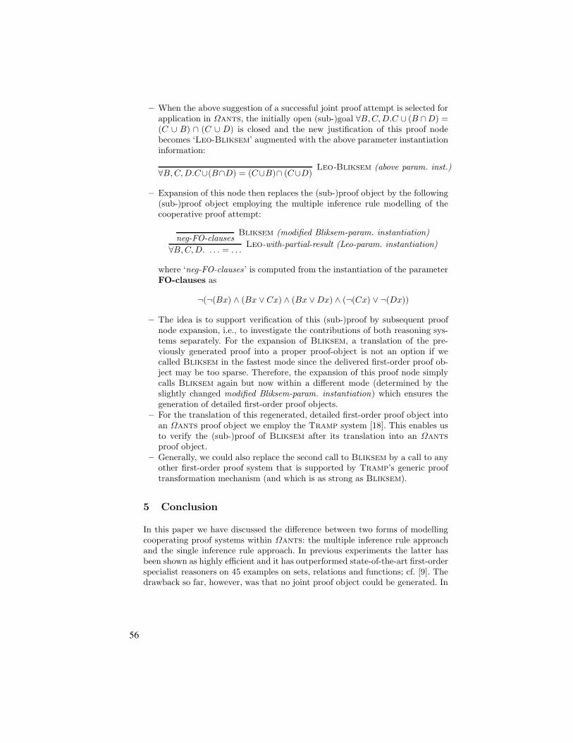
– When the above suggestion of a successful joint proof attempt is selected forapplication in !ants, the initially open (sub-)goal &B, C, D.C " (B #D) =(C " B) # (C " D) is closed and the new justification of this proof nodebecomes ‘Leo-Bliksem’ augmented with the above parameter instantiationinformation:

&B, C, D.C"(B#D) = (C"B)# (C"D)Leo-Bliksem (above param. inst.)

– Expansion of this node then replaces the (sub-)proof object by the following(sub-)proof object employing the multiple inference rule modelling of thecooperative proof attempt:

neg-FO-clausesBliksem (modified Bliksem-param. instantiation)

&B, C, D. . . . = . . .Leo-with-partial-result (Leo-param. instantiation)

where ‘neg-FO-clauses ’ is computed from the instantiation of the parameterFO-clauses as

¬(¬(Bx) ' (Bx % Cx) ' (Bx % Dx) ' (¬(Cx) % ¬(Dx))

– The idea is to support verification of this (sub-)proof by subsequent proofnode expansion, i.e., to investigate the contributions of both reasoning sys-tems separately. For the expansion of Bliksem, a translation of the pre-viously generated proof into a proper proof-object is not an option if wecalled Bliksem in the fastest mode since the delivered first-order proof ob-ject may be too sparse. Therefore, the expansion of this proof node simplycalls Bliksem again but now within a di"erent mode (determined by theslightly changed modified Bliksem-param. instantiation) which ensures thegeneration of detailed first-order proof objects.

– For the translation of this regenerated, detailed first-order proof object intoan !ants proof object we employ the Tramp system [18]. This enables usto verify the (sub-)proof of Bliksem after its translation into an !ants

proof object.– Generally, we could also replace the second call to Bliksem by a call to any

other first-order proof system that is supported by Tramp’s generic prooftransformation mechanism (and which is as strong as Bliksem).

5 Conclusion

In this paper we have discussed the di"erence between two forms of modellingcooperating proof systems within !ants: the multiple inference rule approachand the single inference rule approach. In previous experiments the latter hasbeen shown as highly e!cient and it has outperformed state-of-the-art first-orderspecialist reasoners on 45 examples on sets, relations and functions; cf. [9]. Thedrawback so far, however, was that no joint proof object could be generated. In

56

this paper we have reported how we have solved this problem by simply mappingthe single inference rule modelling back to the multiple inference rule modelling.

Related to our approach is the Techs system [13], which realises a cooper-ation between a set of heterogeneous first-order theorem provers. Similarly toour approach, partial results in Techs are exchanged between the di"erent the-orem provers in form of clauses. The main di"erence to the work of Denzingeret al. (and other related architectures like [14]) is that our system bridges be-tween higher-order and first-order automated theorem proving. Also, unlike inTechs, we provide a declarative specification framework for modelling exter-nal systems as cooperating, concurrent processes that can be (re-)configured atrun-time. Related is also the work of Hurd [16] which realises a generic inter-face between HOL and first-order theorem provers. It is similar to the solutionpreviously achieved by Tramp [18] in Omega, which serves as a basis for thesound integration of ATPs into !ants. Both approaches pass essentially first-order clauses to first-order theorem provers and then translate their results backinto HOL resp. Omega. Some further related work on the cooperation of Is-abelle with Vampire is presented in [19]. The main di"erence of our work tothe related systems is that while our system calls first-order provers from withinhigher-order proof search, this is not the case for [16, 18, 19].

Future work is to investigate how far our approach scales up to more complexproblems and more advanced mathematical theories. In less trivial settings asdiscussed in this paper, we will face the problem of selecting and adding relevantlemmata to avoid immediate reduction to first principles and to appropriatelyinstantiate set variables. Relevant related work for this setting is Bishop’s ap-proach to selectively expand definitions as presented in [10] and Brown’s PhDthesis on set comprehension in Church’s type theory [11].

References

1. P. Andrews. An Introduction to mathematical logic and Type Theory: To Truththrough Proof. Number 27 in Applied Logic Series. Kluwer, 2002.

2. C. Benzmuller. Equality and Extensionality in Higher-Order Theorem Proving.PhD thesis, Universitat des Saarlandes, Germany, 1999.

3. C. Benzmuller. Extensional higher-order paramodulation and RUE-resolution.Proc. of CADE-16, LNAI 1632, p. 399–413. Springer, 1999.

4. C. Benzmuller. Comparing approaches to resolution based higher-order theoremproving. Synthese, 133(1-2):203–235, 2002.

5. C. Benzmuller, M. Jamnik, M. Kerber, and V. Sorge. Experiments with an Agent-Oriented Reasoning System.Proc. of KI 2001,LNAI 2174, p.409--424. Springer, 2001.

6. C. Benzmuller and M. Kohlhase. LEO – a higher-order theorem prover. Proc. ofCADE-15, LNAI 1421. Springer, 1998.

7. C. Benzmuller and V. Sorge. A Blackboard Architecture for Guiding InteractiveProofs. Proc. of AIMSA’98, LNAI 1480, p. 102–114. Springer, 1998.

8. C. Benzmuller and V. Sorge. !ants – An open approach at combining Interactiveand Automated Theorem Proving. Proc. of Calculemus-2000. AK Peters, 2001.

9. C. Benzmuller, V. Sorge, M. Jamnik, and M. Kerber. Can a Higher-Order and aFirst-Order Theorem Prover Cooperate? Proc. LPAR’04, LNAI 3452, Montevideo,Uruguay. Springer, 2005.

57

10. M. Bishop and P. Andrews. Selectively instantiating definitions. Proc. of CADE-

15, LNAI 1421. Springer, 1998.11. C. E. Brown. Set Comprehension in Church’s Type Theory. PhD thesis, Dept. of

Mathematical Sciences, Carnegie Mellon University, USA, 2004.12. H. de Nivelle. The Bliksem Theorem Prover, Version 1.12. Max-Planck-Institut,

Saarbrucken, Germany, 1999. http://www.mpi-sb.mpg.de/ bliksem/manual.ps.13. J. Denzinger and D. Fuchs. Cooperation of Heterogeneous Provers. Proc. IJCAI-

16, p. 10–15. Morgan Kaufmann, 1999.14. M. Fisher and A. Ireland. Multi-agent proof-planning. CADE-15 Workshop “Using

AI methods in Deduction”, 1998.15. H. Ganzinger and J. Stuber. Superposition with equivalence reasoning and delayed

clause normal form transformation. Proc. of CADE-19, LNAI 2741. Springer, 2003.16. J. Hurd. An LCF-style interface between HOL and first-order logic. Automated

Deduction — CADE-18, LNAI 2392, p. 134–138. Springer, 2002.17. M. Kerber. On the Representation of Mathematical Concepts and their Translation

into First Order Logic. PhD thesis, Universitat Kaiserslautern, Germany, 1992.18. A. Meier. TRAMP: Transformation of Machine-Found Proofs into Natural Deduction

Proofs at the Assertion Level. Proc. of CADE-17, LNAI 1831. Springer, 2000.19. J. Meng and L. C. Paulson. Experiments on supporting interactive proof using

resolution. Proc. of IJCAR 2004, LNCS 3097, p. 372–384. Springer, 2004.20. R. Nieuwenhuis, Th. Hillenbrand, A. Riazanov, and A. Voronkov. On the evalua-

tion of indexing techniques for theorem proving. Proc. of IJCAR-01, LNAI 2083,p. 257–271. Springer, 2001.

21. D. Pastre. Muscadet2.3 : A knowledge-based theorem prover based on naturaldeduction. Proc. of IJCAR-01, LNAI 2083, p. 685–689. Springer, 2001.

22. A. Riazanov and A. Voronkov. Vampire 1.1 (system description). Proc. of IJCAR-

01, LNAI 2083, p. 376–380. Springer, 2001.23. V. Sorge. OANTS: A Blackboard Architecture for the Integration of Reasoning Tech-

niques into Proof Planning. PhD thesis, Universitat des Saarlandes, Germany, 2001.24. G. Stenz and A. Wolf. E-SETHEO: An Automated3 Theorem Prover – System

Abstract. Proc. of the TABLEAUX’2000, LNAI 1847, p. 436–440. Springer, 2000.25. G. Sutcli"e and C. Suttner. The TPTP Problem Library: CNF Release v1.2.1.

Journal of Automated Reasoning, 21(2):177–203, 1998.

58

Benchmarks for Higher-Order Automated

Reasoning

Chad E. Brown

Universitat des Saarlandes, Saarbrucken, Germany, cebrown@ags.uni-sb.de

For a higher-order system to be successful it should support users performingtasks both large and small. Large tasks include interactive construction of largetheories, including storing definitions, theorems and proofs. Small tasks includeusing automation to fill in small gaps in proofs. Consider the following theorem:

(C) If f is an n-tuple of complex numbers and fi = 0, then the product f1 · · · fn

of the n-tuple is 0.

In order to even state this theorem, one must first have already defined thecomplex numbers, n-tuples of complex numbers and multiplication of such n-tuples. If one defines the complex numbers using pairs of reals, defines the realsusing Dedekind cuts, and so on, then it is unrealistic to expect a system toautomatically prove this theorem. On the other hand, suppose we include thefollowing as a hypothesis:

(A) Any n-tuple of complex numbers has product 0 i! there exists some jbetween 1 and n such that fj = 0.

Proving the first from the second (i.e., [A ! C]) is a minor exercise in logicand is precisely the sort of gap automation should be able to fill. Such problemsare not trivial, however, since an automated system might consider any numberof irrelevant possibilities during proof search. This is especially true once onebegins expanding definitions.

The example above comes from Jutting’s translation of Landau’s Grundlagender Analysis [6] into Automath [5]. This formalization was recovered and restoredby Wiedijk [7]. We are now in the process of porting the definitions and theoremsfrom the Automath signature into Church’s Type Theory, a form of higher-orderlogic based on simple type theory [2, 4]. However, we are not translating theAutomath proof objects to Church’s Type Theory. Consequently, one obtainsthousands of unproven theorems such as C.

For each such theorem C, one can attempt to prove C in isolation (possi-bly making use of axioms such as description, choice, extensionality or infinity).For most theorems this is unrealistic since the gap between the axioms and thetheorem is simply too wide. On the other hand, one can take all axioms andpreviously proven theorems A1, . . .Am and try to prove C follows from the con-junction of A1, . . .Am. This is generally unrealistic for two reasons. Firstly, theformula becomes too large for automated search once m becomes large. Secondly,if some Ai contains type variables, then one must find a way to instantiate these

59

type variables during the search for a proof. A third alternative is the most real-istic. We provide precisely the relevant axioms and previously proven theorems,with the correct type variable instantiations, and try to prove C follows. In gen-eral, of course, we cannot know which of the Ai’s are relevant. However, for theGrundlagen theorems, we can extract this information from the Automath proofterms. Using this information, we obtain thousands of theorems of the form

[A!

i1" · · · " A!

ik] ! C

where A!

i1is Ai1 with types instantiated appropriately.

Most such theorems correspond to a step given by a single line in the Au-tomath code. For this reason, one can expect most of the theorems to have rea-sonably short proofs. On the other hand, Automath has a stronger type systemthan simple type theory, so one step in Automath may correspond to many stepsin the simply typed version. (Intuitively, what was type checking in Automathbecomes deduction in Church’s type theory.)

This corpus of theorems can be used to empirically test the automated fa-cilities of a higher-order reasoning system. The hope is that such a corpus canprovide reasonable, practical benchmarks for judging the e!ectiveness and e"-ciency of systems and procedures. We report on the initial results of applyingthe theorem prover Tps [1, 3].

References

1. Peter B. Andrews, Matthew Bishop, Sunil Issar, Dan Nesmith, Frank Pfenning,and Hongwei Xi. TPS: A theorem proving system for classical type theory. Journalof Automated Reasoning, 16:321–353, 1996.

2. Peter B. Andrews. An Introduction to Mathematical Logic and Type Theory: To

Truth Through Proof. Kluwer Academic Publishers, second edition, 2002.3. Chad E. Brown. Set Comprehension in Church’s Type Theory. PhD thesis, De-

partment of Mathematical Sciences, Carnegie Mellon University, 2004.4. Alonzo Church. A Formulation of the Simple Theory of Types. Journal of Symbolic

Logic, 5:56–68, 1940.5. L. S. Jutting. Checking Landau’s ”Grundlagen” in the AUTOMATH system. PhD

thesis, Eindhoven Univ., Math. Centre, Amsterdam, 1979.6. E. Landau. Grundlagen der Analysis. Leizig, 1930.7. Freek Wiedijk. A new implementation of Automath. J. Autom. Reasoning, 29(3-

4):365–387, 2002.

60

Co-Synthesis of New Complex SelectionAlgorithms and their Human Comprehensible

XML Documentation

Jutta Eusterbrock

JEusterbrock@seamless-solutions.de

Abstract. In this paper, an approach for program and algorithm syn-thesis within a higher-order framework is presented that allows us togenerate new algorithm structures together with readable documentationwhich enable users to conveniently inspect the results of this synthesisprocess. The synthesis approach is based on feature graphs as a higher-order data type for specifying synthesis types like proof terms, theoremsand document types. The document synthesis method uses constructivereasoning about a user-defined knowledge base to synthesise documentsfrom metaobjects which are composed of diagrams,text, and referencesto articles, theorems and algorithms. The data format used for reasoningis a variant of XML syntax and thus enables the organisation of compre-hensive knowledge in XML repositories and the conversion of documentterms into LATEX, PDF or XHTML documents which can be displayedby browsers.This framework has been applied for the automated synthesis of severalnew selection algorithms and their documentation. As one new result,an algorithm that proves selecting the 4th element of 24 elements needsat most 34 comparisons was synthesised using 50 seconds CPU time onan AMD Athlon 3200. The correctness of the synthesised algorithm wasmanually checked. It improves the known upper bounds for the specificselection problems. The running time for synthesis is several orders ofmagnitude more e!cient than comparative approaches.

1 Introduction

The idea of automatically discovering solutions to mathematical conjectures orproving the non-existence of solutions which are beyond human comprehensionis intriguing. In recent years, computers have been used for a number of famousalgorithmic problems to facilitate analysis based upon a detailed problem specificformalisation. For instance, C. Lam proved that a projective plane of order 10does not exist [Lam91]. As the “proof” took several years of computer search(the equivalent of 2000 hours on a Cray-1), it is considered to be the most time-intensive computer assisted single proof. Recently, G. Gonthier, a mathematicianwho works at Microsoft Research in Cambridge, England, used the CoQ system(cf. [Dev05]) to verify the computer supported proof of the famous Four Color

61

Theorem, which was originally proven in 1976 by Appel and Haken who usedcomputer programs to check a very large number of cases.

However, for a mathematician it is unsatisfying to know that there existsa solution or no solution for a problem, because thousands, hundreds of thou-sands or millions of states have been explored by a theorem prover whose ruleshave been verified, and at the same time, not be able to comprehend the te-dious machine-generated proofs and not be able to draw conclusions from theautomated proof.

In previous work [Eus92b] on automated algorithm synthesis, we designedand implemented a metalevel methodology and system to assist algorithm syn-thesis and the proof of lower complexity bounds. The system evaluated the searchprocess and derived new knowledge which was abstracted and added to a dy-namically growing knowledge base. The system was applied to assist the proofof a number-theoretic conjecture for the selection problem. It was possible toprove the values for very small n within a few minutes on a Sparc Workstation.Surprisingly, the system synthesised an algorithm which constructed a counterexample to a set of rules which should be verified by the system [Eus92a]. Asa side e!ect, an isolated counter-example for a published lower bound for theselection problem was constructed. The computation took several days and themachine generated proofs were cumbersome because the nested proof graphsare hard to comprehend. However, treating proofs as graphs enables variousforms for generating explanations. In [EN96], a visualisation component wasimplemented in order to assist the exploration of huge graphs. Techniques likezooming, organising of graphs on various hierarchy levels, folding and unfoldingtechniques enabled the interactive exploration of large graphs. However, it isassumed that presenting algorithms by documents which are similar to scien-tific or textbook descriptions, making use of di!erent formats and establishinglinks to published results is cognitively more appropriate for proof presentationthan uniform means such as visualisation techniques. Meanwile, XML-based dataformats have emerged as a standard for data encoding and exchange. XML doc-uments can be comparatively easily converted into web pages, LATEX or PDFdocument files which facilitate the display of natural language, graphics, math-ematical symbols and references in an appropriate form.

In this paper, it is illustrated how XML based documentation for automati-cally synthesised algorithms and programs can be generated from specificationsand proof terms and further processed by XML tools is analysed. Synthesisedtheorems and programs should be presented at the right level of granularity suchthat experts can check the automatically synthesised programs in the same wayas they verify a proof in a publication. The key to a solution is abstraction.It is achieved by a higher-order formalisation of abstract synthesis objects anddocument components and a higher-order approach towards automated synthe-sis which raises the level of abstraction (cf. [Kre93]). A method is devised thattransforms program specifications and synthesised algorithms into documentswhich include graphics, text, and references. The method is based upon gen-eral correspondences between synthesis types and document types. User-defined

62

context-specific rules as how to decompose the proof graph, when to generatelemmata and what kind of additional visual information to present at variousstages can be provided. The method has been applied to automatically synthe-sise documents for new complex selection algorithms which were automaticallysynthesised.

The paper is organised as follows. In section 2, the selection problem is in-troduced. Section 3 gives an overview of the synthesis framework. In section 4,the synthesis types and the building blocks of the metatheory for the encod-ing of mathematical knowledge are defined. The document synthesis methodis exlained in section 5. Section 6 summarises some experimental results. Sec-tion 7 concludes this paper. Appendix A contains the automatically synthesiseddocument for the automatically constructed new selection algorithm.

2 The Selection Problem

The selection problem is the problem of finding the i-th largest element, given aset of n distinct unordered numbers, 1 < i < n. The special case i = !n/2" is themedian problem. The worst-case, minimum number of comparisons is denotedby Vi(n). The problem goes back to Rev. C. L. Dodgson’s (aka Lewis Carroll)essay on how prizes were awarded unfairly in tennis tournaments (see Knuth[8:5.33]). In the classic book The Art of Computer Programming, Volume 2,Sorting and Searching [Knu73a], D. Knuth introduces the problem and statesthe combinatorial bounds for n # 10. In [Eus85], the present author constructedthe formula Hi(n)

Hi(n) = n$ i +i!1!

l=1

(!lg(n$ i + 2i$ l + 3

)"+ 2). (1)

It was shown in [Eus85] that the numbers Hi(n) unify the published resultsfor the worst-case behaviour of selection-algorithms as follows. For admissiblecombinations of i, n the numbers Hi(n):

– match the exact numbers Vi(n) for i = 1, 2, 3 [Kis64,Knu73b,Aig82];– are equal to or less than the lower bounds [Kis64,Yao74,FG79,Aig82,MP82,BJ85];– are equal or greater than the upper bounds

[Kis64,HS69,BFP+73,FR75,SPP76,Yap76,Aig82,RH84]

known at that time. Furthermore, using the numbers Hi(n), novel combinatorialalgorithms for small values of i, n were constructed which prove the upper boundsfor small values of i, n:

Vi(n) # Hi(n), i! i # 4, n # 14 and i # 5, n # 12. (2)

The approximate behaviour for the medians is given by the formula below

Hn/2(n) % 2.5n$ 3!lg(n + 4)"+ 5 (3)63

The author stated the hypothesis Vi(n) = Hi(n) for all i, n. For all known upperand lower bounds either Vi(n) & Li(n) or Vi(n) # Ui(n) with one exceptionwhich will be described later on. The hypothetical formula for the median coin-cides with the conjecture of Yao and the conjecture of Paterson Vn/2 % 2.4094n.In [Eus92b] we designed a system in order to assist the refinement of rules. Us-ing this system, it was possible to prove the values for very small n within afew minutes on a Sun Workstation. Surprisingly the system synthesised an al-gorithm which proves V3(22) < H3(22) and thus constructed a counter exampleto a set of rules which should be verified by the system [Eus92a]. The compu-tation took several days. Computerised searches for the selection problem weresubsequently performed by [GKP96] and [Oks05] which use alpha-beta search, atransposition table and some optimisations. Oksanen’s system constructs deci-sion graphs which in summary suggest Vi(n) # Hi(n), i! i # 6, n # 14. However,it is also claimed that V5(12) & 19 = H5(12)$1 while in [Eus85] an algorithm ispresented that proves V5(12) # 18 and thus contradicts the automatically provenstatement. The constructed decision graphs presented in [Oks05] are too largeto comprehend and in the case i = 7, n = 14 consist of more than 600 nodes.

The process for constructing algorithms or lower bounds for selection prob-lems is similar to minimum-comparison sorting. M. Peczarski has devised asystem and analysed the optimal lower bounds S(n) for sorting n elements,n = 13, 14, 22 based on an algorithm for counting the linear extensions of partialorders. The proof S(22) > 70 took 1740 hours on a computer with a 650 MHzprocessor (cf. [Pec04]).

3 The Higher-order Synthesis Framework

In this paper, a reformalisation and reimplementation of our knowledge-basedsynthesis framework, called SEAMLESS (cf. [Eus95]) is analysed. The synthesissystem consists of verified generic methods which take a specification as in-put and generate metalevel proofs by metalevel reasoning about domain-specificknowledge which may be interpreted as programs. The synthesis system evalu-ates the search processes, generalises the case solutions which result from success-ful and failed proof attempts and stores them for further reuse in the knowledgebase. A documentation synthesis component has been added. The document syn-thesis component transforms specifications, derived theorems and synthesisedproofs into XML documents including graphical visualisations, references andtext. The XML documents can be converted by freely available tools into human-readable documents in multiple formats such as XHTML, LATEX or PDF. Theresulting system structure is shown in Figure 1.

In order to achieve an integrated formal framework for the logic-based co-synthesis of proofs and their documentation, principles of a higher-order logic ofprogram synthesis are applied (cf. [Kre93]). The core for the integration of thedi!erent types of knowledge and the correct design of the synthesis methods is ametatheory or, in other terms, an ontology. Types and higher-order predicates torepresent the structure of algorithm design knowledge fragments and properties

64

Fig. 1. Scenario for Knowledge-based Synthesis

or relationships between them have been defined. Figure 2 lists the major typesof the SEAMLESS framework.

Basic types Bool, Integer, Constants, Vars, StringObject logic Atom, Clause, Algebraic Expression, ConstraintSynthesis types Precondition, Postcondition, Program, Proof

Fig. 2. Types for Program Synthesis

In this paper, the notation of [Kre93] is adopted and used in a semi-formalway. A definition New Object Type' Composition of Defined Object Types definesa new object in terms of already existing object types. Meta theorems are writtenin the form Goal ( Subgoal1 ) . . . ) Subgoalr or they are stated as facts.

The Floyd-Hoare logic [Hoa69] is used for specifying the semantics of imper-ative programs and to associate logical specifications with programs. In Floyd-Hoare’s logic, triples of the form {Pre}Prog{Post} state that if program Progstarts in an input state satisfying Pre then if and when Prog halts, it does so ina state satisfying Post. Programs are sequences of statements. Hoare provideda set of logical rules in order to reason about the correctness of computer pro-grams. It is well-known that the Floyd-Hoare rules and axioms can be embeddedin higher order logic and become derived rules. In the SEAMLESS framework,a statement is a variable assignment, procedure or conditional. Loop statementstogether with their specifications can be added to the knowledge base, however,their automatic synthesis is currently not supported as it is based on non-trivial

65

mathematical induction. Consequently, the key conceptual building elementsof the SEAMLESS theory include the abstractions precondition, postcondition,proofs which may be interpreted as programs, and, moreover, range constraintsfor a cost function as part of the postcondition. The metatheory is defined interms of generic predicates and formal axioms for them which provide correctnessaxioms for the suitable domain theories. For example, the correctness axiom forthe higher-order predicate Know states that a proof for the validity of a Hoaretriple is known.

Know(Pre, Post, Prog, True) ' * {Pre}Prog{Post}

Domain-specific design knowledge can be provided by definitions for theopen generic higher-order predicates, if the correctness axioms are satisfied.The SEAMLESS knowledge base of the system entails theorems which are re-lations among truth values, specifications and programs. They are stated ashigher-order theorems, once types for the corresponding abstractions and thesemantics of the higher-order predicates have been defined. In this applicationscenario, the knowledge bases contain published domain specific theorems aboutthe complexity of selection problems, as summarised in section 2, and variousrelated algorithms encoded as arguments of the higher-order predicate Know.The knowledge base of the synthesis system also comprises theorems whose proofis only given by a bibliographic reference to the corresponding document.

Generic synthesis methods have been derived from the generic predicatesas metatheorems. The proofs-as-programs paradigm is adapted to the Hoarelogic for the purpose of extending it to synthesising imperative programs. Asynthesis method is a set of rules including metavariables for programs whichare instantiated while proving the synthesis task. A very basic synthesis strategyis to retrieve solutions from the knowledge base which is specified below.

Synthesis(Pre, Prog, Post, Bool) ( Know(Pre, Prog, Post, Bool)

Experience has shown that theorems as they are published in the literatureare often not directly applicable for solving a problem specification. Equivalences,generalisations, and reductions are considered to establish semantic relationsbetween specifications and the theorems in the literature to obtain proofs. Theserelations can be modelled by corresponding higher-order predicates.

4 Graphterms as a Higher-order Datastructure and XML

The extensible Markup Language (XML) has emerged as a quasi-standard forknowledge exchange, document processing and Web applications. XML is a met-alanguage used to create generalised markup languages. XML annotations facili-tate the retrieval of document fragments based upon their semantic annotations.The focus in this paper is on a more convenient and e"cient data structure thanarbitrary terms for the organisation of the knowledge fragments. The data struc-tures are optimised in order

66

– to facilitate the automatic synthesis of human comprehensible XML-baseddocuments;

– to elicit the interplay between design knowledge - which has been publishedin scientific documents and Web resources - and the corresponding encodingas theorem in the knowledge base of a reasoning system;

– to tackle the huge search complexities.

Linear (serial) term representations, named graphterms, were devised as a datastructure for the encoding of labelled DAGs and feature graphs [Eus97]. Graph-terms (cf. [Eus01,Eus97]) are used as the core data structure to encode formalisedknowledge fragments in SEAMLESS.

Definition 1 Suppose that there are given an infinite set of variables, a set offeatures, and a set of constants. From features, constants attribute variables, andvariables, terms are constructed, if features are seen equivalently as binary pred-icates that must be interpreted as functional relations. Let f be a feature symbol,X a variable. A feature graphterm is an expression f(X, Graphtermlist), whereGraphtermlist is either the empty list [], or denotes a list of constants, variablesand feature graphterms.

To ensure that graphterms are directed acyclic graphs, further axioms constrainthe valid terms. A graphterm algebra, that is term rewriting operations thatimplement graph operations and canonical forms for classes of isomorphic objectswas constructed (cf. [Eus97]). Composed types can be defined using featuregraphs and the objects of a type are instantiated feature graphs. The followingassertion defines a type Spec

Spec([Id = No], [Pre([], [Pre]), Post([], [Post])]) (Conjunction of Atom(Pre) ) Conjunction of Atom(Post).

Each attribute variable of a feature graph may be instantiated by a thuslist ofattributes. In the examples above, specifications are assigned the attribute iden-tifier. Attributes don’t change the logical semantics of the terms, however, theymay be used to design more e"cient synthesis methods. It is possible to attachhash values to a graphterm by means of attributes. Objects may be substitutedby references to them. An algorithm reference can be an automatically generatedcounter, e.g., Alg12345. Then it refers to an automatically generated object inthe knowledge base or it refers to published algorithms, e.g., Kislitsyn,Aignerwhich were constructed outside the synthesis system. The use of references fa-cilitates sharing of terms. It decreases the size of the knowledge base and makesrelationships more obvious. The encoding of knowledge is demonstrated by thehigher-order formula 4.

Know([], P re([], [poset]), P rog([Id = id,Refid = Kislitsyn], []),Post([], [Select(i, poset), Bound(r..r)), T rue) (

i = 2 ) Forest(poset) ) CostK(poset) = r. (4)67

The advantage of using graphterms for encoding higher-order formulas isthat feature graphterms directly correspond to XML Document Type Defini-tions (DTDs) and the instantiated ground terms are syntactic variants of XML(cf. [Eus01]). This facilitates the storing and maintenance of structured designknowledge fragments in XML repositories or XML databases, their retrievalbased upon semantic annotations, and at the same time enables formal reason-ing about them.

5 Higher-order XML-based Document Synthesis

To an increasing degree widely used XML Document Type Definitions like Doc-Book are being used for the structuring and mark-up of software documentationand scientific publications. Common document structuring elements are, for ex-ample, figure, graphics, theorem, proof or enumeration. These XML documentsthen can be transformed into di!erent target formats like LATEX, XHTML orPDF and provided with a professional layout using freely available tools. Docu-ment synthesis is a process that automatically generates a complete structureddocument. In this section, how to synthesise documents, given a program speci-fication and its proof will be examined.

In order to enable constructive synthesis of documentation, a subset of thetbook DTD is used to formalise the types of the theory for document syn-thesis. The tbook DTD was chosen because it is an XML file format that issuitable for scientific texts, but it is also as simple and small as possible, usessimilar names to LATEX and it accepts MathML’s presentation and contentsmarkup. The tbook tools for XML authoring (cf. [Bro05]) may be used totransform the XML document into XHTML, DocBook or LATEX documents.The tbook document types are used in the SEAMLESS knowledge base tomodel document structure. Type definitions are encoded by non-ground factsusing feature graphs as knowledge representation format. The simplified doc-ument type is sketched in Figure 3. Automatic document synthesis is imple-

Document ! Sequence of Header and BodyBody ! Sequence of Theorems or Lemmata and their ProofsTheorem, Lemma ! Sequence of Statements or Enumeration of ItemsProof ! Sequence of Statements or Enumeration of ItemsItem, Statement ! Natural language sentence, Figure, Reference or Algebraic expression

Fig. 3. Simplified Document Type

mented by the generic method Doc synthesis which when invoked by a goal( Doc synthesis([spec,proof],docterm), given a pair [spec,proof], causes the in-stantiation of the metavariable docterm by a document term that describesthe document structure. Scripts are provided that convert document terms oftype document into the corresponding XML syntax. The resulting documents

68

can be processed by the tbook tools. The synthesised method is formalised byhigher-order predicates which relate programming types and document types. Amethod which creates the basic document structure is outlined in Figure 4 andneed to be augmented by the specifications for the methods Doc syn theorem,Doc syn proof , Doc syn lemmata:

– Doc syn theorem synthesises theorem content from formal specifications.– Doc syn proof generates the proof content and a set of proof cases which

shall be treated as lemmata.– Doc syn lemmata generates the presentation for the proof cases.

Doc syn([spec, proof ], doc)" Doc header(header)#Doc body([spec, proof ], body)#doc = Document(att, [header, body]).

Doc body([spec, proof ], body)" Doc theorem(spec, theo)#Doc proof(proof, doc proof, subcases)#Doc syn lemmata(subCases, seq lem proof))#body = Body(att, [theo, doc proof, seq lem proof ].

Fig. 4. Skeleton of the document synthesis method

The above synthesis skeleton prescribes the main structure of the document to besynthesised. Specifications are mapped into theorems and programs into proofs.However, the content of these elements needs to be determined in more detail.It requires the partition of the specifications and their proofs into manageableparts, each part should be presented adequately, avoiding low-level details, butcompiling all the information which is necessary for the comprehension of a proofpart and required to keep the coherence between the parts. Each of the 3 methodsDoc syn theorem, Doc syn proof, Doc syn lemmata is realised as a divide-and-conquer strategy. The specifications of the generic methods consist of metaruleswhich define how to decompose the program synthesis fragments and how tocompose the document fragments. Synthesis involves various decisions whichare based on context-specific knowledge:

– how to decompose the program into subprograms which are represented asone major step;

– when to use graph visualisations or textual explanations for proof parts;– which parts of the proof graph to split and to treat separately as lemmata.

The knowledge base of the document synthesiser can be augmented by heuristiclayout knowledge, e.g., “acceptable” sizes for decision trees. The knowledge baseentails parameterised text templates which are associated with correspondingobjects of the program synthesis theory. The graph visualisation tool graphviz[Res05] is called on demand to generate graph layouts in the desired format.

69

6 Experimental Results

A previous version of SEAMLESS included generic methods for synthesis andmachine learning which were devised independently of the data structure usedfor knowledge encoding. Domain specific knowledge was provided through an in-termediate component as definitions for open generic predicates. The system wasused to prove V3(22) # 28 which constructed a counter example for a publishedtheorem. Although the time for constructing the algorithm that has verifiedV3(22) # 28 was not exactly measured, the computation had taken several dayson a Sun Solaris workstation.

The system has been partially reimplemented by reusing the formally correctgeneric methods, however, changing the implementation of the data structuresand the knowledge representation format. The knowledge representation schemaand graph-based data structure which have been devised in this paper have beenused to structure and implement the specialised domain knowledge about theselection problem. Indexing techniques for graphs have been introduced to tacklethe huge search complexities structure. The results of these changes are

1. a radical improvement of the search complexities;2. more abstract well-defined metalevel proofs with a higher degree of reuse

which is reflected by references and links to objects and theorems;3. a clearer distinction between informal or formal knowledge which has been

derived outside of the system and automatically derived knowledge.

This implementation was used to re-synthesise algorithms for small n and itcould be automatically proven that Vi(n) # Hi(n), 1 # i # 6, 1 # n # 14.In addition, the implementation was used to automatically synthesise variousnew complex algorithms which prove V4(21) # 30, V4(23) # 33, V4(24) # 34,V4(25) # 35 and V4(26) # 26 and confirm the number-theoretic hypothesis forthe selection problem.

The re-implementation was experimentally analysed on an Athlon 3200 64bit computer with 1 GB memory and on a 1.3 GHZ Intel Centrino laptop with512 MB memory. In this experimental application scenario, Yap Prolog turnedout to be the fastest Prolog compared against Sicstus, GNU, B and SWI Prolog.In Figure 6 some complexity indicators for automated synthesis are collected: 1)a small example whose solution is described in the classic book by Knuth; 2) amore complex example; 3) the previously discovered selection algorithm whichtook days and now can be handled within seconds; 4) much more complex prob-lems whose solutions improve the known upper bounds and confirm the statedhypothesis. The test environment was as follows: a) Centrino + Yap Prolog, b)Centrino + SWI Prolog, c) Athlon 3200 + Yap Prolog, d) Athlon 3200 + SWIProlog. Some experimental results are summarised in Figure 5. The CPU timeis measured in seconds. During the synthesis process, for each case solution, acanonical form is computed that represents the solution up to isomorphism. Theabstracted case solutions can be reused and adapted. The number of generatedcase solutions for isomorphism classes is given in the last column of the table. Amissing entry means that a solution couldn’t be constructed within a couple of

70

hours. It should be noted that these indicators are snapshots of an implementa-tion in progress. Each minor modification may alter the search space. This candecrease or increase the complexities to solve a problem drastically.

Spec a b c d #examined isomorphism classesV4(7) $ 10 0.026 0.05 0.014 0.01 68V3(22) $ 28 1.87 8.6 0.84 2.93 3,062V4(14) $ 21 9.0 56.0 3.3 18.1 12,122V4(21) $ 30 52.0 996.4 19.3 321.2 61,859V4(23) $ 33 288.9 16,239.7 107.1 5,210.2 277,178V4(24) $ 34 136.8 6,163.3 50.4 1,951.6 127,572V4(25) $ 35 390.4 – 146.5 13,034.3 362,458V4(26) $ 36 – – 525.1 – 1,048,665

Fig. 5. Complexity indicators for correct search

In all experimental analysed cases, it can be experimentally verified thatreuse of derived knowledge from previous proof searches when solving new prob-lems improves the search complexities by up to 25%. Although the system isable to examine around 1,500,000 isomorphic states in less than one half hourand store them in 1 GB memory, the complexities of the selection problem fairlysoon exceed the capabilities of the system. The experiments also showed thatwhen using the computers to full capacity, odd runtime errors occur, e.g., unin-stantiated variables, which cannot attributed to programming errors.

The reuse and knowledge-based synthesis approach generates proof graphswhose size has been decreased enormously compared to the uniform approaches.However, taking the constructed selection algorithms, in most of the more com-plex cases, the sizes of the generated decision graphs are still unsatisfying, be-cause they cannot be manually checked with reasonable e!ort.

The generic synthesis method is based upon a 3-valued logic. Heuristic know-ledge marked with the truth value Maybe can be provided. In order to decreasethe sizes of the proof graphs various incorrect lower bounds were experimentallyadded to the knowledge base. The simplest form of an incorrect lower boundis a depth restriction. The incorrect lower bounds restrict the search space.Employing these heuristics, an unsuccesful search may yield the result Maybe.Using heuristic search a solution for V4(24) # 34 could be constructed within 6.5secs, having examined 13695 isomorphism classes and having used Yap Prologon the AMD Athlon 3200. The size of this proof graph was also substantiallydecreased.

The generated graph is still too large to be easily comprehensible, thereforeit is embedded in a system-generated documentation which provides a mathe-matically skilled reader background information about the proofs, such as caseswhich can be reduced to problems known from the literature, or are solved usingthe dedicated lemmata. The automatically synthesised documentation of thisautomatically synthesised algorithm is presented in appendix A.

71

A major advantage of combining higher-order program synthesis and doc-ument synthesis is that the generated proof terms describe programs at thealgorithmic abstraction level. There is no need to raise the level of abstractionor to integrate a planning module into the document synthesis component. Thesynthesised document is a direct mapping from specifications and proofterms. Animproved knowledge base of the system directly causes an improved documen-tation. Comprehensibility depends on the size of the automatically synthesisedproof graphs. For small i, n the automated co-synthesis of algorithms and theirdocumentation achieves human-comprehensible documents. For complex prob-lems, synthesis of proof terms of reasonable sizes is an experimental endeavour.

7 Conclusions and Related Work

In [Kre93], it has been stated “We believe that a formalization of the metatheoryof programming is one of the most important steps towards the development ofprogram synthesisers which are flexible and reliable and whose derivations areboth formally correct and comprehensible for human programmers.” As a steptowards this objective, this paper has experimentally analysed the interplay be-tween mathematical documents and knowledge-based algorithm synthesis basedupon a metatheory for structuring problem solving knowledge. Structuring ele-ments are identified to formalise algorithm design knowledge which is implicit inscientific documents and include abstractions like pre- and postconditions basedupon the Floyd-Hoare program logics. Types, higher-order predicates and syn-thesis methods have been defined. The resulting framework is more fine-grainedthan related approaches for program synthesis which are based upon higher-order logic or proof planning [Kre93,IS04,RicCA]. The SEAMLESS frameworkalso aims at the formalisation of heuristic problem solving strategies and resourcerestrictions. The framework devised has been applied to structure comprehensiveknowledge relating to the selection problem and encode it for use in a knowledgebase. The knowledge base has been used for the synthesis of complexity boundedalgorithms using generic methods that were previously devised. Extended graph-terms are used as the core data structure for knowledge encoding. They providethe key for the e"ciency of the implementation as they support various optimi-sation techniques. The huge search complexities are tackled by a combinationof indexing techniques, isomorphism abstraction, machine learning and knowl-edge reuse through references. It was possible to synthesise several new complexselection algorithms which improve known bounds and confirm our hypothesis.

Based upon the higher-order synthesis framework, a method that synthe-sises human-comprehensible XML-based documents from specifications and con-structed proofs has been devised and implemented. The synthesised documentsinclude diagrams and references to reused knowledge. The method has been ap-plied for the automatic synthesis of documentation for automatically synthesisedalgorithms. It allows logic-based synthesis of documents on a higher abstractionlevel than a number of current low-level XML-based approaches which aim at theexchange or presentation of arbitrary mathematical documents, Website synthe-

72

sis or program documentation and merely exploit the correspondences betweenXML data and logical terms, e.g., [BDHG,LR03,SR01]. The presented frameworkdistinguishes itself from related approaches (cf. [Pec04,GKP96,Oks05]) in whichcomputer have been used for the complexity analysis of unsolved mathematicalproblems. The results synthesised by SEAMLESS are constructive, comprehen-sible and can be manually checked for correctness, provided that the sizes of thegenerated proof graphs are reasonable. In one case, it was possible to synthe-sise a new complex algorithm of reasonable length, and, thus the synthesiseddocumentation is comprehensible (cf. Appendix A).

Our future work will include experimental work on automated abstractionto decrease the size of the generated algorithms and to get more abstract ex-planations for series of single proof steps or comprehensive decision trees. Theobjective is to discover a few rules which describe new correct algorithms forinfinitely many n.

References

[Aig82] M. Aigner. Selecting the top three elements. Discrete Applied Mathematics,4:247–267, 1982.

[BDHG] Dietmar A. Seipel, Bernd D. Heumesser and Ulrich Guntzer. An expertsystem for the flexible processing of XML-based mathematical knowledge ina Prolog-environment.

[BFP+73] M. Blum, R.W. Floyd, V. Pratt, R.L. Rivest, and R.E. Tarjan. Time boundsfor selection. J. Comp. Syst. Sci., 7:448–461, 1973.

[BJ85] S.W. Bent and J.W. John. Finding the median requires 2n comparisons. InProc. 17th ACM Symposium Theory of Computing, pages 213–216, 1985.

[Bro05] Torsten Bronger. The tbook system for XML authoring.http://tbookdtd.sourceforge.net, 25.9.2005.

[Dev05] Keith Devlin. Last doubts removed about the proof of the four color theorem.http://www.maa.org/devlin/devlin 01 05.html, January 2005.

[EN96] J. Eusterbrock and M. Nicolaides. The visualization of constructive proofsby compositional graph layout: A world-wide web interface. Proc. CADEVisual Reasoning Workshop, Rutgers University, 1996.

[Eus85] J. Eusterbrock. Ein rekursiver Ansatz zur Bestimmung der Anzahl vonVergleichen bei kombinatorischen Selektionsproblemen. Diplomarbeit, Uni-versitat Dortmund, 1985.

[Eus92a] J. Eusterbrock. Errata to “Selecting the top three elements” by M. Aigner:A Result of a computer assisted proof search. Discrete Applied Mathematics,41:131–137, 1992.

[Eus92b] J. Eusterbrock. Wissensbasierte Verfahren zur Synthese mathematischerBeweise: Eine kombinatorische Anwendung, volume 10 of DISKI, 1992.

[Eus95] J. Eusterbrock. SEAMLESS: Knowledge based evolutionary system synthe-sis. ERCIM News, 23, October 1995.

[Eus97] J. Eusterbrock. Canonical term representations of isomorphic transitiveDAGs for e!cient knowledge-based reasoning. In Proceedings of the In-ternational KRUSE Symposium, Knowledge Retrieval, Use and Storage forE!ciency, pages 235–249, 1997.

73

[Eus01] J. Eusterbrock. Knowledge mediation in the world-wide web based uponlabelled dags with attached constraints. Electronic Transactions on ArtificialIntelligence, 5:”http://www.ida.liu.se/ext/epa/ej/etai/2001/D”, 2001.

[FG79] F. Fussenegger and H.N. Gabow. A counting approach to lower bounds forselection problems. J. Assoc. Comput. Mach., 26:227–238, 1979.

[FR75] R.W. Floyd and R.L. Rivest. Expected time bounds for selection. Comm.ACM, 18:165–172, 1975.

[GKP96] William Gasarch, Wayne Kelly, and William Pugh. Finding the ith largestof n for small i,n. SIGACT News, 27(2):88–96, 1996.

[Hoa69] C.A.R. Hoare. An axiomatic basis for computer programming. CACM,12(10):576–581, 1969.

[HS69] A. Hadian and M. Sobel. Selecting the t-th largest using binary errorlesscomparisons. In P. Erdos, A. Renyi, and V.T. Sos, editors, CombinatorialTheory and its Applications II, pages 585–600. North Holland, 1969.

[IS04] A. Ireland and J. Stark. Combining proof plans with partial order planningfor imperative program synthesis. Journal of Automated Software Engineer-ing, Accepted for publication, 2004.

[Kis64] S. S. Kislitsyn. On the selection of the k-th element of an ordered set bypairwise comparisons. Sib. Mat. Z., 5:557–564, 1964.

[Knu73a] D.E. Knuth. Fundamental algorithms, volume 1 of The Art of ComputerProgramming. Addison Wesley, Reading, MA, 1973.

[Knu73b] D.E. Knuth. Sorting and Searching, volume 3 of The Art of Computer Pro-gramming. Addison Wesley, Reading, MA, 1973.

[Kre93] Chr. Kreitz. Metasynthesis - deriving programs that develop programs. Ha-bilitationsschrift, Technische Hochschule Darmstadt, 1992.

[Lam91] Clement Lam. The search for a finite projective plane of order 10. AmericanMathematical Monthly, 98:305–318, 1991.

[LR03] S. Leung and D. Robertson. Automated website synthesis.http://www.ukuug.org/events/linux2003/papers/leung.pdf, 2003.

[MP82] J.I. Munro and P.V. Poblete. A lower bound for determining the median.Technical report, University of Waterloo Research Report CS-82-21, 1982.

[Oks05] Kenneth Oksanen. Selecting the ith largest of n elements.http://www.cs.hut.fi/ cessu/selection/, 2005.

[Pec04] Marcin Peczarski. New results in minimum comparison sorting. Algorith-mica, 40:133–145, 2004.

[Res05] AT&T Research. Graphviz - graph visualization software.http://www.graphviz.org/, 25.9.2005.

[RH84] P.V. Ramanan and L. Hyafil. New algorithms for selection. J. of Alg.,1:557–578, 1984.

[RicCA] C.S Richardson, J.D. Proof planning and program synthesis: a survey. InLogic-Based Program Synthesis: State-of-the-Art & Future Trends, AAAI2002 Spring Symposium, March 25-27, 2002, Stanford University, CA.

[SPP76] A. Schonhage, M. Paterson, and N. Pippenger. Finding the median. J.Comp. System Sci., 13:184–199, 1976.

[SR01] Johann Schumann and Peter Robinson. [] or success is notenough: Current technology and future directions in proof presentation.http://www.cs.bham.ac.uk/ mmk/events/ijcar01-future/, 2001.

[Yao74] F.F. Yao. On lower bounds for selection problems. Technical report, TR-121,MIT, Project Mac, Cambridge, Mass., 1974.

[Yap76] C.K. Yap. New upper bounds for selection. Comm. ACM, 19:501–508, 1976.

74

A Automatically Synthesised Documentation1

Select(4,24)

c!Jutta Eusterbrock

theorem 1 V4(24) $ 34

Proof. Let KEYS be a totally ordered set, |KEY S| = 24. The 4 -th largest element ofKEYS is computed by Algorithm 1. The computation takes in the worst-case at most34 comparisons.

algorithm 1

1. Partition the set KEYS into disjoint subsets |K1| = 16, |K2| = 8. Determine themaxima of K1,K2 by setting-up balanced tournaments. The resulting poset is iso-morphic to the poset as shown in Figure 6. For setting-up the balanced tournaments22 comparisons are needed.

a1

a9 a5 a3 a2

a13 a11 a10 a7 a6 a4

a15 a14 a12

a16

a8

a17

a21 a19 a18

a23 a22 a20

a24

Fig. 6. Balanced Tournaments of Set Partition

1This is an automatically composed documentation of a new, automaticallysynthesised algorithm Select(4, 24) with the worst-case complexity V4(24) ! 34.Based on the proof structure derived during the synthesis, the system selected,instantiated, and composed appropriate text templates to generate the explanatorytext and document structure. The graphs were visualised by the graphviz system. Theproof was checked for correctness by the present author.

75

2. Perform the comparisons in accordance with the decision graph in Figure 7. Thenodes in the decision graph represent:(a) Comparisons X : Y , shown as circles. The left child node represents the case

X > Y and the right one the case X < Y .(b) Subgraph place holders, shown by references to a diamond which correspond

to solutions which can be obtained by instantiating theorems and algorithmsknown from published literature. The cases 1, 27, 48, 49, 739, 743, 744, 873,874, 7772, 7773, 7823, 7824, 7839, 7840 are instances of published theorems.

(c) Place holders for calls to simplification functions, especially isomorphism func-tions, which are denoted by boxes. There are two type of function calls. Firstly,solutions for the simplified subcases are represented by a subgraph which is thenreferenced. This concerns case 7844. Secondly, in some situations more detailedexplanations for the simplified subcases, e.g, lemmata, have been generated. Inthe given decision graph, the cases 876 and 7775 are handled separately.

a9-a17

a17-a5

a3-a19

a17-a3 a13-a3 a3-a21

7844

1

a13-a3 a13-a5 a9-a5

kislitsyn

[5, 40.0] 27

a9-a3

[4, 12.0] 48 49

[4, 12.0] [3, 18.0]

739

a9-a5 a9-a3 876

[4, 20.0] 743 744

[4, 20.0] [4, 20.0]

873 874

[5, 16.0] [3, 18.0]

a3-a5 a5-a21

a17-a3 7775 a17-a5 a1-a21

7772 7773

[4, 26.0] [4, 22.0]

7823 7824 7839 7840

[4, 18.0] [4, 12.0] [4, 26.0] [4, 20.0]

Fig. 7. Decision Tree

3. Generate solutions for specific cases:– Case 876 is described as follows. Let P be the poset as visualised in Figure 8. It

needs to be proven V3(P ) $ 8. The specification is up-to-isomorphism handledby Lemma 1.

– Case 7775 is described as follows. Let P be the poset as visualised in Figure 9. Itneeds to be proven V3(P ) $ 8. The specification is up-to-isomorphism handledby Lemma 2.

76

a5

a6 a7 a9

a8 a10 a11 a17

a3

a4

a12 a18 a19 a21

a2

a20 a22 a23

a24

Fig. 8. Poset P

a5

a3 a6 a7

a4 a8

a17

a18 a9

a10 a11 a13

a2

a12 a14 a15

a16

Fig. 9. Poset P

lemma 1 Let P be a poset as visualised in Figure 10. The 3-rd largest element of Pcan be computed by at most 8 comparisons.

Proof. algorithm 2

1. Compare a9 and a3.(a) a9 > a3. a9 is greater than the 3-rd largest element and is reduced. The result-

ing poset P satisfies the precondition of the algorithm [Kis64]. Hence, selectingthe 2-nd largest element takes at most f(5,14.0)=7 comparisons.

(b) a9 < a3. a3 is greater than the 3-rd largest element and is reduced. The result-ing poset P satisfies the precondition of the algorithm [Kis64]. Hence, selectingthe 2-nd largest element takes at most f(3,10.0)=5 comparisons.

77

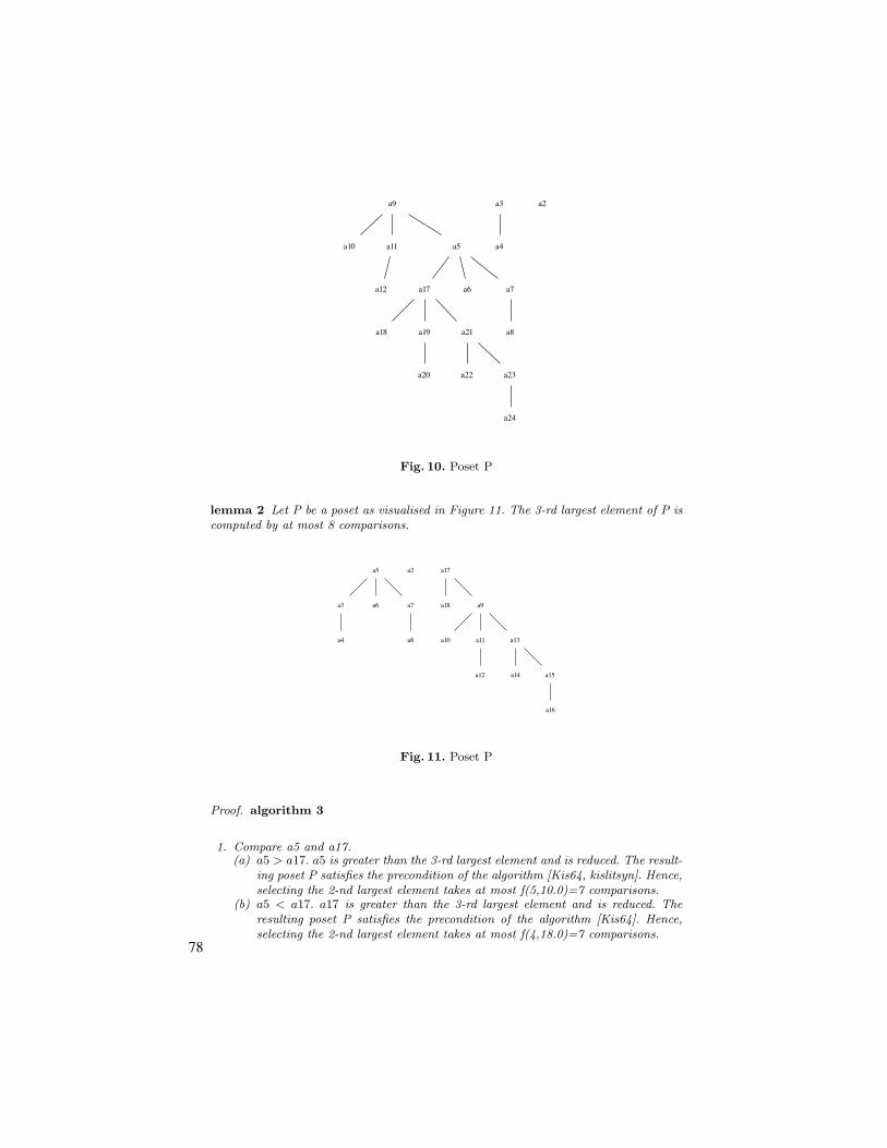
a9

a10 a11 a5

a12 a17 a6 a7

a3

a4

a18 a19 a21 a8

a2

a20 a22 a23

a24

Fig. 10. Poset P

lemma 2 Let P be a poset as visualised in Figure 11. The 3-rd largest element of P iscomputed by at most 8 comparisons.

a5

a3 a6 a7

a4 a8

a2 a17

a18 a9

a10 a11 a13

a12 a14 a15

a16

Fig. 11. Poset P

Proof. algorithm 3

1. Compare a5 and a17.(a) a5 > a17. a5 is greater than the 3-rd largest element and is reduced. The result-

ing poset P satisfies the precondition of the algorithm [Kis64, kislitsyn]. Hence,selecting the 2-nd largest element takes at most f(5,10.0)=7 comparisons.

(b) a5 < a17. a17 is greater than the 3-rd largest element and is reduced. Theresulting poset P satisfies the precondition of the algorithm [Kis64]. Hence,selecting the 2-nd largest element takes at most f(4,18.0)=7 comparisons.

78

Mixing Finite Success and Finite Failure

in an Automated Prover

Alwen Tiu1, Gopalan Nadathur2, and Dale Miller3

1 INRIA Lorraine/LORIA2 Digital Technology Center and Dept of CS, University of Minnesota

3 INRIA & LIX, Ecole Polytechnique

Abstract. The operational semantics and typing judgements of mod-ern programming and specification languages are often defined using re-lations and proof systems. In simple settings, logic programming lan-guages can be used to provide rather direct and natural interpreters forsuch operational semantics. More complex features of specifications suchas names and their bindings, proof rules with negative premises, and theexhaustive enumeration of state spaces, all pose significant challengesto conventional logic programming systems. In this paper, we describea simple architecture for the implementation of deduction systems thatallows a specification to interleave between finite success and finite fail-ure. The implementation techniques for this prover are largely commonones from higher-order logic programming, i.e., logic variables, (higher-order pattern) unification, backtracking (using stream-based computa-tion), and abstract syntax based on simply typed !-terms. We present aparticular instance of this prover’s architecture and its prototype imple-mentation, Level 0/1, based on the dual interpretation of (finite) successand finite failure in proof search. We show how Level 0/1 provides a high-level and declarative implementation of model checking and bisimulationchecking for the (finite) "-calculus.

1 Introduction

The operational semantics and typing judgements of modern programming andspecification languages are often defined using relations and proof systems, e.g.,in the style of Plotkin’s structural operational semantics. In simple settings,higher-order logic programming languages, such as !Prolog and Twelf, can beused to provide rather direct and natural interpreters for operational seman-tics. However, such logic programming languages can provide little more thananimation of semantic descriptions: in particular, reasoning about specified lan-guages has to be done outside the system. For instance, checking bisimulationin process calculi needs analyzing all the transition paths a process can poten-tially go through. To add to the complication, modern language specificationsoften make use of complex features such as variable bindings and the notionof names (as in the "-calculus [MPW92]), which interferes in a non-trivial waywith case analyses. These case analyses cannot be done directly inside the logic

79

programming system, not in a purely logical way at least, even though they aresimply enumerations of answer substitutions. In this paper, we describe an ex-tension to logic programming with logically sound features which allow us to dosome modest automated reasoning about specifications of operational semantics.This extension is more conceptual than technical, that is, the implementation ofthe extended logic programming language uses only implementation techniquesthat are common to logic programming, i.e., logic variables, higher-order patternunification, backtracking (using stream-based computation) and abstract syntaxbased on typed !-calculus.

The implementation described in this paper is based on the logic FO!!!

[MT03], which is a logic based on a subset of Church’s Simple Theory of Typesbut extended with fixed points and the ! quantifier. In FO!!! quantificationover propositions is not allowed but quantifiers can otherwises range over vari-ables of higher-types. Thus the terms of the logic can be simply typed terms,which can be used to encode the !-tree syntax of encoded objects in an opera-tional semantics specification. This style of encoding is a variant of higher-orderabstract syntax in which meta-level !-abstractions are used to encode object-level variable binding. The quantifier ! is first introduced in [MT03] to helpencode the notion of “generic judgment” that occurs commonly when reasoningwith !-tree syntax.

The logical extension to allow fixed points is done through a proof theoreticalnotion of definitions [SH93,Eri91,Gir92,Sta94,MM00]. In a logic with definitions,an atomic proposition may be defined by another formula (which may containthe atomic proposition itself). Proof search for a defined atomic formula is doneby unfolding the definition of the formula. A provable formula like "X.pX # qX ,where p and q are some defined predicates, expresses the fact that for every termt for which there is a successful computation (proof) of pt, there is a computation(proof) of qt. Towards establishing the truth of this formula, if the computationtree associated with p is finite, we can e!ectively enumerate all its computationpaths and check the provability of qt for each path. Note that if the computationtree for p is empty (pt is not provable for any t) then "X.pX # qX is (vacuously)true. In other words, failure in proof search for pX entails success in proof searchfor pX # qX . The analogy with negation-as-failure in logic programming isobvious: if we take qX to be $ (false), then provability of pX # $ corresponds tosuccess in proof search for not(pX) in logic programming. This relation betweennegation-as-failure in logic programming and negation in logic with definitionshas been observed in [HSH91,Gir92]. In the implementation of FO!!!, theabove observation leads to a neutral view on proof search: If proof search for agoal A returns a non-empty set of answer substitutions, then we have found aproof of A. On the other hand, if proof search for A returns an empty answer set,then we have found a proof for ¬A. Answer substitutions can thus be interpretedin a dual way depending on the context of proof search; see Section 3 for moredetails.

The rest of the paper is organized as follows. In Section 2, we give an overviewof the logic FO!!!. Section 3 describes an implementation of a fragment of

80

FO!!!, the Level-0/1 prover, which is based on a dual interpretation of fail-ure/success in proof search. Section 4 discusses the treatment of variables in theLevel-0/1 prover, in particular, it discusses the issues concerning the interactionbetween eigenvariables and logic variables. Section 5 specifically contrasts theexpressiveness of Level-0/1 over what is available in !Prolog. Section 6 gives aspecification of the operational semantics for the "-calculus and shows how Level-0/1 can turn that specification naturally into a checker for (open) bisimulation.Section 7 provides a specification of modal logic for the "-calculus, which theLevel-0/1 prover can use to do model checking for that process calculus. Thesetwo specifications involving the "-calculus illustrate the use of the !-quantifierto help capture various restrictions of names in the "-calculus. Section 8 dis-cusses the components of proof search implementation and outlines a generalimplementation architecture for FO!!!. Section 9 discusses future work. Anextended version of this paper is available on the web, containing more exam-ples and more detailed comparison with logic programming.

2 Overview of the logic FO!!!

The logic FO!!! [MT03] (pronounced “fold-nabla”) is presented using a se-quent calculus that is an extension of Gentzen’s system LJ [Gen69] for intuition-istic logic. The first extension to LJ is to allow terms to be simply typed !-termsand to allow quantification to be over all types not involving the predicate type(in Church’s notation [Chu40], the types of quantified variables do not containo). A sequent is an expression of the form B1, . . . , Bn % B0 where B0, . . . , Bn

are formulas and the elongated turnstile % is the sequent arrow. To the left ofthe turnstile is a multiset: thus repeated occurrences of a formula are allowed. Ifthe formulas B0, . . . , Bn contain free variables, they are considered universallyquantified outside the sequent, in the sense that if the above sequent is prov-able then every instance of it is also provable. In proof theoretical terms, suchfree variables are called eigenvariables. Eigenvariable can be used to encode thedynamics of abstraction in the operational semantics of various languages. How-ever, for reasoning about certain uses of abstraction, notably the notion of namerestriction in "-calculus, eigenvariables do not capture faithfully the intendedmeaning of such abstractions. To address this problem, in the logic FO!!! se-quents are extended with a new notion of “local scope” for proof-level boundvariables (see [MT03] for motivations and examples). In particular, sequents inFO!!! are of the form

# ; $1 %B1, . . . ,$n %Bn % $0 %B0

where # is a global signature, i.e., the set of eigenvariables whose scope is overthe whole sequent, and $i is a local signature, i.e., a list of variables scoped overBi. We shall consider sequents to be binding structures in the sense that thesignatures, both the global and local ones, are abstractions over their respectivescopes. The variables in # and $i will admit &-conversion by systematicallychanging the names of variables in signatures as well as those in their scope,

81

#, $ ! t : % # ; $ & B[t/x], ' " C

# ; $ & #!x.B, ' " C#L

#, h ; ' " $ & B[(h $)/x]

# ; ' " $ & #x.B#R

#, h ; $ & B[(h $)/x], ' " C

# ; $ & $x.B,' " C$L

#, $ ! t : % # ; ' " $ & B[t/x]

# ; ' " $ & $!x.B$R

# ; ($, y) & B[y/x], ' " C

# ; $ & %x B, ' " C%L

# ; ' " ($, y) & B[y/x]

# ; ' " $ & %x B%R

Fig. 1. The introduction rules for quantifiers in FO!"!.

following the usual convention of the !-calculus. The meaning of eigenvariablesis as before, only that now instantiation of eigenvariables has to be capture-avoiding, with respect to the local signatures. The variables in local signaturesact as locally scoped generic constants, that is, they do not vary in proofs sincethey will not be instantiated. The expression $ %B is called a generic judgmentor simply a judgment. We use script letters A, B, etc., to denote judgments. Wewrite simply B instead of $ %B if the signature $ is empty.

The logical constants of FO!!! are "" (universal quantifier), &" (existen-tial quantifier), !" (nabla quantification), ' (conjunction), ( (disjunction), #(implication), ) (true) and $ (false). The subscript for the three quantifiers isthe type of the variable they are intended to bind: in particular, ' can rangeover any type not containing the predicate type. Usually this type subscript issuppressed. The inference rules for the three quantifiers of FO!!! are given inFigure 1. The introduction rules for propositional connectives are straightfor-ward generalization of LJ: in particular, local signatures are distributed over thesubformulas of the main formula (reading the rules bottom-up). The completeset of rules for FO!!! is given in Figure 10 at the end of this paper.

During the search for proofs (reading rules bottom up), the right-introductionrule for " and the left-introduction rule for & place new variables into the globalsignature: the left and right introduction rules for ! place new variables into thelocal signature. In the "R and &L rules, raising [Mil92] is used when replacingthe bound variable x, which can range over the variables in both the globalsignature and the local signature $, with the variable h that can only rangeover variables in the global signature: so as not to miss substitution terms, thevariable x is replaced by the term (h x1 . . . xn), which we shall write simply as(h$), where $ is the list x1, . . . , xn (h must not be free in the lower sequent ofthese rules). In "L and &R, the term t can have free variables from both # and$. This is presented in the rule by the typing judgment #,$ * t : '. The !Land !R rules have the proviso that y is not free in !x B.

Besides these introduction rules for logical constants, FO!!! additionallyallows the introduction of atomic judgments, that is, judgments of the form$ %A where A is an atomic formula. To each atomic judgment, A, we associatea judgment B called the definition of A. The introduction rule for the judgmentA is in e!ect done by replacing A with B during proof search. This notion of

82

definitions is an extension of work by Schroeder-Heister [SH93], Eriksson [Eri91],Girard [Gir92], Stark [Sta94] and McDowell and Miller [MM00] and allows formodest reasoning about the fixed points of definitions.

Definition 1. A definition clause is written "x[p t"= B], where p is a predicate

constant, every free variable of the formula B is also free in at least one termin the list t of terms, and all variables free in p t are contained in the list x ofvariables. The atomic formula p t is called the head of the clause, and the formula

B is called the body. The symbol"= is used simply to indicate a definitional

clause: it is not a logical connective.

Let ""1x1 . . .""n

xn.H"= B be a definition clause. Let y1, . . . , ym be a list of

variables of types &1, . . . ,&m, respectively. The raised definition clause of H withrespect to the signature {y1 : &1, . . . , ym : &m} is defined as

"h1 . . . "hn.y %H("= y %B(

where ( is the substitution [(h1 y)/x1, . . . , (hn y)/xn] and hi is of type &1 +. . . + &m + 'i. A definition is a set of definition clauses together with theirraised clauses.

The introduction rules for a defined judgment are displayed below. Whenapplying the introduction rules, we shall omit the outer quantifiers in a definitionclause and assume implicitly that the free variables in the definition clause aredistinct from other variables in the sequent.

{#( ; B(,)( % C( | ( , CSU(A,H) for some clause H"= B}

# ; A,) % C defL

# ; ) % B(# ; ) % A def R, where H

"= B is a definition clause and H( = A

In the above rules, we apply substitutions to judgments. The result of applyinga substitution ( to a generic judgment x1, . . . , xn % B, written as (x1, . . . , xn %B)(, is y1, . . . , yn % B#, if (!x1 . . .!xn.B)( is equal (modulo !-conversion) to!y1 . . .!yn.B#. If ) is a multiset of generic judgments, then )( is the multiset{J( | J , )}. In the defL rule, we use the notion of complete set of unifiers(CSU) [Hue75]. We denote by CSU(A,H) a complete set of unifiers for the pair(A,H), that is, for any unifier ( of A and H, there is a unifier * , CSU(A,H)such that ( = * - (# for some substitution (#. Since we allow higher-order termsin definitions, in certain cases there are no finite CSU’s for a given unificationproblem. Thus, in the fully general case, defL may have an infinite number ofpremises [MM00]. In all the applications of defL in this paper, however, theterms involved in unification are those of higher-order patterns [Mil91,Nip93],that is, terms in which variables are applied only to distinct bound variables.Since higher-order pattern unification is decidable and unary (i.e., the mostgeneral unifiers exist if the unification is solvable), the set CSU(A,H) in this

83

case can be treated as being either empty or containing a single substitutionwhich is the most general unifier. In this restricted setting, defL will have afinite number of premises (assuming as we shall that definitions are based onthe raising of only a finite number of clauses). The signature #( in defL denotesthe signature obtained from # by removing the variables in the domain of (and adding the variables in the range of (. In the defL rule, reading the rulebottom-up, eigenvariables can be instantiated in the premise, while in the def R

rule, eigenvariables are not instantiated. The set that is the premise of the defLrule means that that rule instance has a premise for every member of that set:if that set is empty, then the premise is considered proved.

One might find the following analogy with logic programming helpful: if adefinition is viewed as a logic program, then the def R rule captures backchainingand the defL rule corresponds to case analysis on all possible ways an atomicjudgment could be proved. The latter is a distinguishing feature between theimplementation of FO!!! discussed in Section 3 and logic programming. Forinstance, given the definition

{pa"= ), pb

"= ), qa

"= ), qb

"= ), qc

"= )},

one can prove "x.px # qx: for all successful “computation” of p, there is asuccessful computation for q. Notice that by encoding logic programs as defini-tions, one can e!ectively encode negation-as-failure in logic programming usingdefL [HSH91], e.g., for the above program (definition), the goal not(pc) in logicprogramming is encoded as the formula pc # $.

Two properties of FO!!! are particularly important to note here. First, ifa certain stratification of predicates within definitions is made (so that thereis no circularity in defining predicates through negations) then cut-eliminationand consistency can be proved [MT05,Tiu04]. Second, many inference rules areknown to be invertible, in the sense that they can always be applied withoutthe need for backtracking. Those rules include defL, !L, !R, &L, "R, the rightintroduction rules for ' and #, and the left introduction rules for ' and ([Tiu04]. The invertibility of these rules motivates the choice of the fragment ofFO!!! on which the Level-0/1 prover works.

3 Mixing success and failure in a prover

We now give an overview of an implementation of proof search for a fragmentof FO!!!. This implementation, called Level 0/1 prover, is based on the dualinterpretation of finite success and finite failure in proof search. In particular,the finite failure in proving a goal &x.G should give us a proof of ¬(&x.G) andvice versa. We experiment with a simple class of formulas which exhibits thisduality. We first assume that all predicate symbols are classified as belonging toeither level-0 or level-1 (via some mapping of predicates to {0, 1}). Next consider

84

the following classes of formulas:

Level 0: G := ) | $ | A | G ' G | G ( G | &x.G | !x.GLevel 1: D := ) | $ | A | D ' D | D ( D | &x.D | !x.D | "x.D | G # Datomic: A := p t1 . . . tn

Here, atomic formulas A in level 0 formulas must have predicates that have beenassigned to level 0. Atomic formulas in level 1 formulas can have predicates of

either level 0 and 1. Each definition clause pt"= B must be stratified, i.e., if p

is a level-0 predicate then B should belong to the class level-0, otherwise if pis a level-1 predicate then B can be a level-0 or level-1 formula. In the currentimplementation, stratification checking and type checking are not implemented,so that we can experiment with a wider range of definitions than those for whichthe meta-theory is fully developed.

Notice that in the Level-1 formula, the use of implication is restricted to theform G # D where G is a Level-0 formula. Therefore, nested implication like(A # B) # C is not allowed. The Level-0/1 prover actually consists of two sepa-rate subprovers, one for each class of formulas. Implementation of proof search forlevel-0 formula follows the standard logic-programming implementation for Hornclauses: it is actually the subset of !Prolog based on Horn clauses but allowingalso ! quantification in the body of clauses. In this prover, existential quantifiersare instantiated with logic variables, !-quantifiers are instantiated with scoped(local) constants (which have to be distinguished from eigenvariables), and def Ris implemented via backchaining. For level-1 formulas, the non-standard case iswhen the goal is an implication, e.g., G # D. Proof search strategy for this casederives from the following observation: the left-introduction rules for level-0 for-mulas are all invertible rules, and hence can always be applied first. Proof searchfor an implicational goal G # D therefore proceeds as follows:

Step 1 Run the level-0 prover with the goal G, treating any level-1 eigenvari-ables as level-0 logic variables.

Step 2 Collect all answer substitutions produced by Step 1 into a lazy streamof substitutions and for each substitution ( in this stream, proceed withproving G(. For example, if Step 1 fails, then this stream is empty and thisstep succeeds immediately.

In Step 1, we impose a restriction: the formula G must not contain any occur-rences of level-1 logic variables. If this restriction is violated, a runtime exceptionis returned and proof search is aborted. We shall return to this technical restric-tion in Section 4. This restriction on the occurrence of logic variable has notposed a problem for a number of applications, e.g., checking bisimulation andsatisfiability of modal logic formulas for the "-calculus.

We claim the following soundness theorem for the provers architecture above:If Level-0/1 is given a definition and a goal formula and it successfully claimsto have a proof of that goal (that is, the system terminates without a runtimeerror), then that goal follows from the definition also in the FO!!! logic.

85

Concrete syntax The concrete syntax for Level 0/1 prover follows the syntax of!Prolog. The concrete syntax for logical connectives are as follows:

) true $ false' & (ampersand) or , (comma) ( ; (semi-colon)" pi & sigma! nabla # =>

The !-abstraction is represented in the concrete syntax using an infix back-slash, with the body of a !-abstraction is goes as far to the right as possible,consistent with the existing parentheses: for example, !x!f.fx can be writtenas (x\f\ f x). The order of precedence for the connectives is as follows (indecreasing order): ', (, #, {", &,!}. Follow the convention started by Church[Chu40], the bound variable associated to a quantifier is actually a !-abstraction:for example, the logical expression "x[p(x) # q(x)]' p(a) can be encoded as the(pi x\ p x => q x) & (p a). Non-logical constants, such as ‘not’ (negation-as-failure) and ‘!’ (Prolog cut), are not implemented, while we do allow thenon-logical constant print for printing terms. Finally, we note that the percentsign % starts a comment line.

The symbol"= separating the head and the body of a definition clause is writ-

ten as ‘:=’ in the concrete syntax. For example, the familiar ‘append’ predicatefor lists can be represented as the following definition.

append nil L L.

append (cons X L1) L2 (cons X L3) := append L1 L2 L3.

As in !Prolog, we use ‘.’ (dot) to indicate the end of a formula. Identifiersstarting with a capital letter denote variables and those starting with lower-caseletter denote constants. Variables in a definition clause are implicitly quantifiedoutside the clause (the scope of such quantification is over the clause, so thereis no accidental mixing of variables across di!erent clauses). A definition clausewith the body ‘true’ is abbreviated with the ‘true’ removed, e.g., the first clauseof append above is actually an abbreviation of append nil L L := true.

4 Eigenvariables, logic variables and !

The three quantifiers, ", & and !, give rise to three kinds of variables dur-ing proof search: eigenvariables, logic variables and “variables” generated by !.Their characteristics are as follows: logic variables are genuine variables, in thatthey can be instantiated during proof search. Eigenvariables are subject to in-stantiation only in proving negative goals, while in positive goals they are treatedas scoped constants. Variables generated by ! are never instantiated and areusually represented by !-abstractions. Eigenvariables and logic variables sharesimilar data structures, and explicit raising is used to encode their dependencyon !-variables. The interaction between eigenvariables and logic variables is

86

more subtle. Consider the case where both eigenvariables and logic variables arepresent in a negative goal, for example, consider proving the goal

"x.&y.(px ' py ' x = y # $),

where p is defined as {pa"= ), pb

"= ), pc

"= )}. In proof search for this formula,

we are asked to produce for each x, a y such that x and y are distinct. This is nolonger a unification problem in the usual sense, since we seek to cause a failurein unification, instead of success. This type of problem is generally referred to ascomplement problems or disunification [LC89], and its solution is not unique ingeneral, even for the first-order case, e.g., in the above disunification problem, ifx is instantiated to a then y can be instantiated with either b or c. In the higher-order case [MP03] the problem is considerably more di"cult, and, hence, in thecurrent implementation, we disallow occurrences of logic variables in negativegoals.

In Figure 2, we show a sample session in Level 0/1 prover which highlightsthe di!erences between eigenvariables, logic variables, and !-variables. The uni-fication problem in the first two goals can be seen as the unification problem!x.x = !x.(Mx). Notice that there is no di!erence between " and ! if the goalis level-0 (i.e., there is no implication in the goal). A non-level 0 goal is given inthe third example. Here the unification fails (hence the goal succeeds) becausex is bound in the scope of where M is bound. It is similar to the unificationproblem !x.x = !x.M. Here substitution must be capture-avoiding, thereforeM cannot be instantiated with x. However, if we switch the order of quantifieror using application-term (as in (fx) in the fourth goal) the unification succeeds.In the last goal, we are trying to prove implicational goal with logic variables,and the system returns an exception.

5 Comparison with !Prolog

Setting aside the ! quantifier, one might think that the proof search behavior for" and # connectives in FO!!! can be approximated in !Prolog with negation-as-failure. As we outline below, only in some weak settings can !Prolog naturallycapture the deduction intended in FO!!!.

The # connective, for instance, might be defined in !Prolog as

imp A B :- not(A, not(B)).

If proof search for A terminates with failure, then the goal imp A B succeeds.Otherwise, for each answer substitution for A, if B fails then the whole goal fail,otherwise the not(B) fails and hence imp A B succeeds. For ground terms A and B(thus, containing no eigenvariables), this coincides with the operational readingof A => B in Level 0/1 prover. The story is not so simple, however, if there areoccurrences of eigenvariables in A or B.

One can sort of see intuitively why the inclusion of eigenvariables in A or Bwould cause problem: the eigenvariables in !Prolog play a single role as scoped

87

?- nabla x\ x = (M x).

YesM = x1\x1Find another? [y/n] yNo.

?- pi x\ x = (M x).YesM = x1\x1

Find another? [y/n] yNo.?- pi M\ nabla x\ x = M => false.

YesFind another? [y/n] yNo.

?- pi f\ nabla x\ x = f x => print "unification succeeded".unification succeededYes

?- nabla x\ pi y\ x = y => print "unification succeeded".unification succeededYes

?- nabla x\ x = (M x) => false.Error: non-pure term found in implicational goal.

Fig. 2. A session in Level 0/1 prover.

constant, while in Level 0/1 they have dual roles, as constants and as variablesto be instantiated. However, there is one trick to deal with this, that is, supposewe are to prove "x.Ax # Bx, instead of the straightforward encoding of " as pi,we may use sigma instead:

sigma x\ not (A x, not (B x)).

Here the execution of the goal forces the instantiation of the (supposed to be)‘eigenvariable’. The real problem appears when eigenvariables may assume tworoles at the same time. Consider the goal

"x"y.x = a # y = b

where a and b are constants. Assuming nothing about the domain of quantifi-cation, this goal is not provable. Now, the possible encodings into !Prolog is touse either sigma or pi to encode the quantifier. Using the former, we get

sigma x\ sigma y\ not (x = a, not(y = b)).

This goal is provable, hence it is not the right encoding. If instead we use pi toencode ", we get

pi x\ pi y\ not (x = a, not (y = b)).

88

This goal also succeeds, since x here will become an eigenvariable and hence itis not unifiable with a. Of course, one cannot rule out other more complicatedencodings, e.g., treating " as pi in one place and as sigma in others, but itis doubtful that there will be an encoding scheme which can be generalized toarbitrary cases.

6 Example: the "-calculus and bisimulation

An implementation of one-step transitions and strong bisimulation for the "-calculus [MPW92] are given in this section. More details on the adequacy of theencodings presented in this section can be found in [TM04,Tiu04]. We consideronly finite "-calculus, that is, the fragment of "-calculus without recursion orreplication. The syntax of processes is defined as follows

P ::= 0 | xy.P | x(y).P | +.P | (x)P | [x = y]P | P|Q | P + Q.

We use the notation P, Q, R, S and T to denote processes. Names are denotedby lower case letters, e.g., a, b, c, d, x, y, z. The occurrence of y in the processx(y).P and (y)P is a binding occurrence, with P as its scope. The set of freenames in P is denoted by fn(P), the set of bound names is denoted by bn(P). Wewrite n(P) for the set fn(P) . bn(P). We consider processes to be syntacticallyequivalent up to renaming of bound names. The operator + denotes the choiceoperator: a process P +Q can behave either like P or Q. The operator | denotesparallel composition: the process P |Q consists of subprocesses P and Q runningin parallel. The process [x = y]P behaves like P if x is equal to y. The processx(y).P can input a name through x, which is then bound to y. The processxy.P can output the name y through the channel x. Communication takes placebetween two processes running in parallel through the exchanges of messages(names) on the same channel (another name). The restriction operator (), e.g.,in (x)P , restricts the scope of the name x to P .

One-step transition in the "-calculus is denoted by P#

%%+ Q, where P and Qare processes and & is an action. The kinds of actions are the silent action + ,the free input action xy, the free output action xy, the bound input action x(y)and the bound output action x(y). Since we are working with the late transitionsemantics [MPW92], we shall not be concerned with the free input action. Thename y in x(y) and x(y) is a binding occurrence. Just like we did with processes,we use fn(&), bn(&) and n(&) to denote free names, bound names, and names in&. An action with a binding occurrences of a name is a bound action, otherwiseit is a free action.

We encode the syntax of process expressions using !-tree syntax as follows.We shall require three primitive syntactic categories: n for names, p for processes,and a for actions, and the constructors corresponding to the operators in "-calculus. The translation from "-calculus processes and transition judgments to!-tree syntax is given in Figure 3. Figure 4 shows some example processes in !-tree syntax. The definition clauses corresponding to the operational semantics of

89

z : p in : n & (n & p) & p out, match : n & n & p & p

plus : p & p & p par : p & p & p taup : p & p

nu : (n & p) & p tau : a up : n & n & a

dn : n & n & a one : p & a & p & o onep : p & (n & a) & (n & p) & o

[[0]] = z [[[x = y]P]] = match x y [[P]][[xy.P]] = out x y [[P]] [[x(y).P]] = in x !y.[[P]][[P + Q]] = plus [[P]] [[Q]] [[P|Q]] = par [[P]] [[Q]][[(.P]] = taup [[P]] [[(x)P]] = nu !x.[[P]]

[[P#

""& Q]] = one [[P]] tau [[Q]] [[Pxy

""& Q]] = one [[P]] (up x y) [[Q]]

[[Px(y)""& Q]] = onep [[P]] (dn x) (!y[[Q]]) [[P

x(y)""& Q]] = onep [[P]] (up x) (!y[[Q]])

Fig. 3. Encoding the "-calculus syntax with !-tree syntax.

example 0 (nu x\ match x a (taup z)).example 1 (par (in x y\z) (out x a z)).

example 2 (in x u\ (plus (taup (taup z)) (taup z))).example 3 (in x u\ (plus (taup (taup z))

(plus (taup z) (taup (match u y (taup z)))))).

example 4 (taup z).example 5 (nu x\ (par (in x y\z) (out x a z))).example 6 (in x u\ nu y\ ((plus (taup (taup z))

(plus (taup z) (taup (match u y (taup z))))))).

Fig. 4. Several examples processes written in Level-0/1 syntax.

"-calculus are given in Figure 5. The original specification of the late semanticsof "-calculus can be found in [MPW92]. We note that various side conditions onnames and their scopes in the inference rules in the original specification are notpresent in the encoding in Figure 5 since these are handled directly by the useof !-tree syntax and the FO!!! logic.

We consider some simple examples involving one-step transitions, using theexample processes in Figure 4. We can, for instance, check whether a process isstuck, i.e., no transition is possible from the given process. Consider example 0in Figure 4 which corresponds to the process (x)[x = a]+.0. This process clearlycannot make any transition since the name x has to be distinct with respect tothe free names in the process. This is specified as follows

?- example 0 P, (pi A\pi Q\ one P A Q => false),

(pi A\pi Q\ onep P A Q => false).Yes

Recall that we distinguish between bound-action transition and free-action tran-sition, and hence there are two kinds of transitions to be verified.

90

onep (in X M) (dn X) M. % bound input

one (out X Y P) (up X Y) P. % free outputone (taup P) tau P. % tauone (match X X P) A Q := one P A Q. % match prefix

onep (match X X P) A M := onep P A M.one (plus P Q) A R := one P A R. % sumone (plus P Q) A R := one Q A R.

onep (plus P Q) A M := onep P A M.onep (plus P Q) A M := onep Q A M.one (par P Q) A (par P1 Q) := one P A P1. % par

one (par P Q) A (par P Q1) := one Q A Q1.onep (par P Q) A (x\par (M x) Q) := onep P A M.onep (par P Q) A (x\par P (N x)) := onep Q A N.

% restrictionone (nu x\P x) A (nu x\Q x) := nabla x\ one (P x) A (Q x).onep (nu x\P x) A (y\ nu x\Q x y) := nabla x\ onep (P x) A (y\ Q x y).

% openonep (nu y\M y) (up X) N := nabla y\ one (M y) (up X y) (N y).% close

one (par P Q) tau (nu y\ par (M y) (N y)) :=sigma X\ onep P (dn X) M & onep Q (up X) N.

one (par P Q) tau (nu y\ par (M y) (N y)) :=

sigma X\ onep P (up X) M & onep Q (dn X) N.% commone (par P Q) tau (par R T) := sigma X\ sigma Y\ sigma M\

onep P (dn X) M & one Q (up X Y) T & (R = (M Y)).one (par P Q) tau (par R T) := sigma X\ sigma Y\ sigma M\

onep Q (dn X) M & one P (up X Y) R & (T = (M Y)).

Fig. 5. Definition of one-step transitions of finite late "-calculus

bisim P Q :=(pi A\ pi P1\ one P A P1 => sigma Q1\ one Q A Q1 & bisim P1 Q1) &

(pi X\ pi M\ onep P (dn X) M => sigma N\ onep Q (dn X) N &pi w\ bisim (M w) (N w)) &

(pi X\ pi M\ onep P (up X) M => sigma N\ onep Q (up X) N &

nabla w\ bisim (M w) (N w)) &(pi A\ pi Q1\ one Q A Q1 => sigma P1\ one P A P1 & bisim Q1 P1) &(pi X\ pi N\ onep Q (dn X) N => sigma M\ onep P (dn X) M &

pi w\ bisim (N w) (M w)) &(pi X\ pi N\ onep Q (up X) N => sigma M\ onep P (up X) M &

nabla w\ bisim (N w) (M w)).

Fig. 6. Definition of open bisimulation

91

We now consider a notion of equivalence between processes, called bisimu-lation. It is formally defined as follows: a relation R is a bisimulation, if it is asymmetric relation such that for every (P, Q) , R,

1. if P#

%%+ P# and & is a free action, then there is Q# such that Q#

%%+ Q# and(P#, Q#) , R,

2. if Px(z)%%+ P# and z /, n(P, Q) then there is Q# such that Q

x(z)%%+ Q# and for every

name y, (P#[y/z], Q#[y/z]) , R,

3. if Px(z)%%+ P# and z /, n(P, Q) then there is Q# such that Q

x(z)%%+ Q# and (P#, Q#) ,

R.

Two processes P and Q are strongly bisimilar if there is a bisimulation R such that(P, Q) , R. The above definition is also called late bisimulation in the literature.

Consider the definition of the bisim predicate Figure 6 that is inspired bythe above definition. Notice that the di!erence between bound-input and bound-output actions is captured by the use of " and ! quantifiers. This definitionprovides a sound encoding of late bisimulation, meaning that if bisim P Q isprovable then P and Q are late-bisimilar. This encoding turns out to soundand complete for open bisimulation [San96], a finer bisimulation relation thanlate bisimulation (see [TM04] for details of the encoding and adequacy results).The following example, taken from [San96], illustrates the incompleteness withrespect to late bisimulation.

P = x(u).(+.+.0 + +.0), Q = x(u).(+.+.0 + +.0 + +.[u = y]+.0).

This example fails because to prove their bisimilarity, one needs to do caseanalysis on the input name u above, i.e., whether it is equal to y or not, andsince our current prover implements intuitionistic logic, this case split based onthe excluded middle is not available. However, if we restrict the scope of y sothat it appears inside the scope of u, then [u = y] is trivially false. In this case,the processes would be x(u).(+.+.0+ +.0) and x(u).(y)(+.+.0+ +.0+ +.[u = y]+.0),which correspond to example 3 and 6 in Figure 4. They can be proved bisimilar.

?- example 2 P, example 6 Q, bisim P Q.Yes

One should compare the above declarative specification and its implementationof symbolic bisimulation checking with that found in, say, [BN96].

7 Example: modal logics for "-calculus

We now consider the modal logics for "-calculus introduced in [MPW93]. In ordernot to confuse meta-level (FO!!!) formulas (or connectives) with the formulas(connectives) of modal logics under consideration, we shall refer to the latteras object formulas (respectively, object connectives). We shall work only withobject formulas which are in negation normal form, i.e., negation appears only

92

top : o", bot : o", and : o" & o" & o", or : o" & o" & o"

boxMatch : n & n & o" & o", diaMatch : n & n & o" & o",boxAct : a & o" & o", diaAct : a & o" & o",boxInL : n & (n & o") & o", diaInL : n & (n & o") & o"

boxOut : n & (n & o") & o", diaOut : n & (n & o") & o"

sat : p & o" & o.

[[true]] = top [[false]] = bot[[A ' B]] = and [[A]] [[B]] [[A ( B]] = or [[A]] [[B]][[[x = y]A]] = boxMatch x y [[A]] [[)x = y*A]] = diaMatch x y [[A]][[))*A]] = diaAct ) [[A]] [[[)]A]] = boxAct ) [[A]][[)x(y)*LA]] = diaInL x (!y[[A]]) [[[x(y)]LA]] = boxInL x (!y[[A]])[[)x(y)*A]] = diaOut x (!y[[A]]) [[[x(y)]A]] = boxOut x (!y[[A]])[[P |= A]] = sat [[P]] [[A]]

Fig. 7. Translation from modal formula to !-tree syntax.

at the level of atomic object formulas. As a consequence, we introduce explicitlyeach dual pair of the object connectives. Note that since the only atomic objectformulas are either true or false, we will not need negation as a connective (since¬true 0 false and ¬false 0 true). The syntax of the object formulas is given by

A ::= true | false | A ' A | A ( A | [x = z]A | 1x = z2A| 1&2A | [&]A | 1x(y)2A | [x(y)]A | 1x(y)2LA | [x(y)]LA

Here, & denotes a free action, i.e., it is either + or xy. The modalities [x(y)]L

and 1x(y)2L are the late bound-input modalities, and 1x(y)2 and [x(y)] are thebound output modalities. There are other variants of input and output modal-ities considered in [MPW93] which we do not represent here. For the completeencoding of the modal logics, we refer the interested readers to [Tiu05]. In eachof the formulas (and their dual ‘boxed’-formulas) 1x(y)2A and 1x(y)2LA, the oc-currence of y in parentheses is a binding occurrence whose scope is A. Objectformulas are considered equivalent up to renaming of bound variables. We shallbe concerned with checking whether a process P satisfies a given modal formulaA. This satisfiability judgment is written as P |= A. The translation from modalformulas and judgments to !-tree syntax is given in Figure 7.

The satisfiability relation for the modal logic is encoded as the definitionclauses in Figure 8. For the original specification, we refer the interested readersto [MPW93]. The definition in Figure 8 is not complete, in the sense that thereare true assertion of the modal logic which are not provable using this definitionalone. For instance, the modal judgment

x(y).x(z).0 |= 1x(y)2L1x(z)2L(1x = z2true ( [x = z]false)

which basically says that two names are either equal or not equal, is valid, butits encoding in FO!!! is not provable since the meta logic is intuitionistic. Acomplete encoding of the modal logic is given in [Tiu05] by explicitly introducingaxioms for the excluded-middle on name equality, namely, "x"y[x = y ( x /= y].

93

sat P top.sat P (and A B) := sat P A, sat P B.

sat P (or A B) := sat P A; sat P B.sat P (boxMatch X Y A) := (X = Y) => sat P A.sat P (diaMatch X Y A) := (X = Y), sat P A.

sat P (boxAct X A) := pi P1\ one P X P1 => sat P1 A.sat P (diaAct X A) := sigma P1\ one P X P1, sat P1 A.sat P (boxOut X A) := pi Q\ onep P (up X) Q => nabla y\ sat (Q y) (A y).

sat P (diaOut X A) := sigma Q\ onep P (up X) Q, nabla y\ sat (Q y)(A y).sat P (boxInL X A) := pi Q\ onep P (dn X) Q => sigma y\ sat (Q y) (A y).sat P (diaInL X A) := sigma Q\ onep P (dn X) Q, pi y\ sat (Q y) (A y).

Fig. 8. Specification of a modal logic for "-calculus.

The definition in Figure 8 serves also as a model checker for "-calculus. Forinstance, consider the processes 2 and 6 given by in Figure 4. We have seen thatthe two processes are bisimilar. A characterization theorem given in [MPW93]states that (late) bisimilar processes satisfy the same set of modal formulas. Weconsider a particular case here. The modal formula

1x(y)2L(1+21+2true ( 1+2true)

naturally corresponds to the process 2. In the concrete syntax, this formula iswritten as follows

assert (diaInL x (y\ or (diaAct tau (diaAct tau top))(diaAct tau top))).

We show that both processes 2 and 6 satisfy this formula.

?- assert A, example 2 P, example 6 Q, sat P A, sat Q A.Yes

8 Components of proof search implementation

Implementation of proof search for FO!!! is based on a few simple key com-ponents: !-tree syntax, i.e., data structures for representing objects containingbinding, higher-order pattern unification, and stream-based computation. Thefirst two are implemented using the suspension calculus [NW98], an explicitsubstitution notation that allows computations over !-terms to be realized flex-ibly and e"ciently; further details of the implementation used may be found in[NL05]. We explain the last component briefly. We use streams to store answersubstitutions, which are computed lazily, i.e., only when they are queried. Thedata type for stream in the ML language is shown in Figure 9. Here the typeustream is a polymorphic stream. The element of a stream is represented as thedata type cell, which can be a delayed cell or a forced cell. A delayed cell stores

94

an unevaluated expression, and its evaluation is triggered by the call to the func-tion getcell. A forced cell is an element which is already a value. Elements ofa stream are initially created as delayed cells. Note that since an element of astream can also be a (cell of) stream, we can encode di!erent computation pathsusing streams of streams. This feature is used, in a particular case, to encodethe notion of backtracking in logic programming.

datatype ’a cell = delayedcell of unit -> ’a | forcedcell of ’atype ’a elm = ’a cell

datatype ’a ustream = empty | ustream of ’a * (’a ustream elm ref)fun getcell(t as ref(delayedcell t’)) =

let val v = t’() in (t := (forcedcell v); v) end

| getcell(ref (forcedcell v)) = vfun mkcell t = ref(delayedcell t)

Fig. 9. The stream datatype in ML.

A stream of substitutions for a given goal stores all answer substitutions forthe goal. In logic programming, such answer substitutions can be queried oneby one by users. Often we are interested in properties that hold for all answersubstitutions. For instance, in bisimulation checking for transition systems, aswe have seen in the "-calculus example, one needs to enumerate all possiblesuccessors of a process and check bisimilarity for each successor. In some otherexamples, information on failed proof search attempts could be of interest aswell, e.g., generating counter-model in model checking. This motivates the choiceof implementation architecture for FO!!!: various fragments of FO!!! areimplemented as (specialized) automated provers which interact with one another.For the current implementation, interaction between provers are restricted toexchanging streams of answer substitutions. A particular arrangement of theinteraction between provers that we found quite useful is what we call a "&-interaction. In its simplest form, this consists of two provers, as exemplifiedin the Level-0/1 prover. Recall that in Level-0/1 prover, a proof search sessionconsists of Level-1 calling the Level-0 prover, extracting all answer substitutions,and for each answer substitutions, repeating the calling cycle until the goals areproved. At the implementation level, one can generalize the provers beyond twolevels using the same implementation architecture. For instance, one can imagineimplementing a “Level-2 prover” which extracts answers from a Level-1 proverand perform some computations on them. Using the example of "-calculus, aLevel-2 prover would, for instance, allow for proving goals like “P and Q are notbisimilar”. This would be implemented by simply calling Level-1 on this goaland declare a success if Level-1 fails.

95

9 Future work

The current prover implements a fairly restricted fragment of the logic FO!!!.We consider extending it to richer fragments to include features like, amongothers, induction and co-induction proof rules (see, e.g.,[Tiu04]) and arbitrarystratified definition (i.e., to allow more nesting of implications in goals). Ofcourse, with induction and co-induction proofs, there is in general no completeautomated proof search. We are considering implementing a circular proof searchto automatically generates the (co)inductive invariants. Works along this line hasbeen studied in, e.g., [SD03]. This extended feature would allow us, for example,to reason about bisimulation of non-terminating processes. Another possibleextension is inspired by an on going work on giving a game semantics for proofsearch, based on the duality of success and failure in proof search. Our particularproof search strategy for Level-0/1 prover turns out to correspond to certain "&-and &"-strategies in the game semantics in [MS05]. The game semantics studiedthere also applies to richer fragments of logics. It would be interesting to see ifthese richer fragments can be implemented as well using a similar architectureas in Level-0/1 prover.

We also plan to use more advance techniques to improve the current im-plementation such as using tabling to store and reuse subproofs. The use oftabled deduction in higher-order logic programming has been studied in [Pie03].It seems that the techniques studied there are applicable to our implementation,to the Level-0 prover at least, since it is a subset of !Prolog. Another possi-ble extension would be a more flexible restriction on the occurrence of logicvariables. The current prover cannot yet handle the case where there is a caseanalysis involving both eigenvariables and logic variables. Study on a notion ofhigher-order pattern disunification [MP03] would be needed to attack this prob-lem at a general level. However, we are still exploring examples and applicationswhich would justify this additional complication to proof search. We also planto study more examples on encoding process calculi and the related notions ofbisimulations.

Acknowledgements. Support has been obtained for this work from the followingsources: from INRIA through the “Equipes Associees” Slimmer, from the ACIgrants GEOCAL and Rossignol and from the NSF Grant CCR-0429572 that alsoincludes support for Slimmer.

References

[BN96] Michele Boreale and Rocco De Nicola. A symbolic semantics for the "-calculus. Information and Computation, 126(1):34–52, April 1996.

[Chu40] Alonzo Church. A formulation of the simple theory of types. J. of SymbolicLogic, 5:56–68, 1940.

[Eri91] Lars-Henrik Eriksson. A finitary version of the calculus of partial induc-tive definitions. In L.-H. Eriksson, L. Hallnas, and P. Schroeder-Heister,editors, Proc. of the Second International Workshop on Extensions to LogicProgramming, volume 596 of LNAI, pages 89–134. Springer-Verlag, 1991.

96

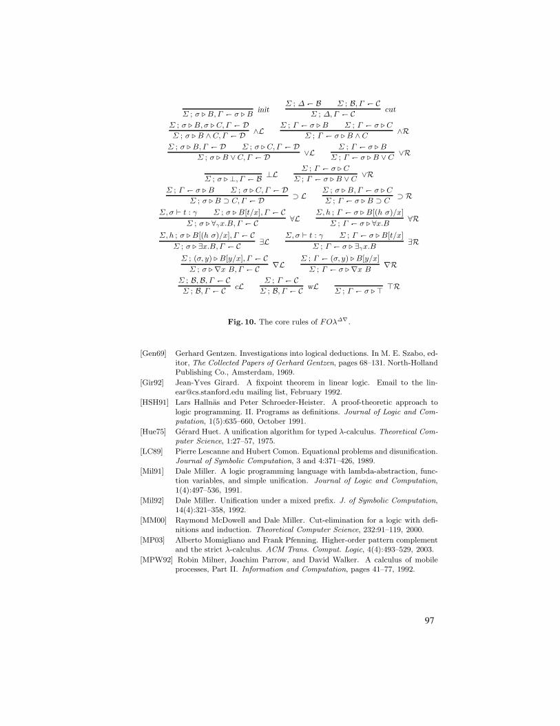
# ; $ & B, ' " $ & Binit

# ; * " B # ; B, ' " C

# ; *, ' " Ccut

# ; $ & B, $ & C, ' " D

# ; $ & B ' C, ' " D'L

# ; ' " $ & B # ; ' " $ & C

# ; ' " $ & B ' C'R

# ; $ & B, ' " D # ; $ & C, ' " D

# ; $ & B ( C, ' " D(L

# ; ' " $ & B

# ; ' " $ & B ( C(R

# ; $ & +, ' " B+L

# ; ' " $ & C

# ; ' " $ & B ( C(R

# ; ' " $ & B # ; $ & C, ' " D

# ; $ & B , C, ' " D, L

# ; $ & B, ' " $ & C

# ; ' " $ & B , C, R

#, $ ! t : % # ; $ & B[t/x], ' " C

# ; $ & #!x.B, ' " C#L

#, h ; ' " $ & B[(h $)/x]

# ; ' " $ & #x.B#R

#, h ; $ & B[(h $)/x], ' " C

# ; $ & $x.B,' " C$L

#, $ ! t : % # ; ' " $ & B[t/x]

# ; ' " $ & $!x.B$R

# ; ($, y) & B[y/x], ' " C

# ; $ & %x B, ' " C%L

# ; ' " ($, y) & B[y/x]

# ; ' " $ & %x B%R

# ; B,B, ' " C

# ; B, ' " CcL

# ; ' " C

# ; B, ' " CwL

# ; ' " $ & --R

Fig. 10. The core rules of FO!"!.

[Gen69] Gerhard Gentzen. Investigations into logical deductions. In M. E. Szabo, ed-itor, The Collected Papers of Gerhard Gentzen, pages 68–131. North-HollandPublishing Co., Amsterdam, 1969.

[Gir92] Jean-Yves Girard. A fixpoint theorem in linear logic. Email to the lin-ear@cs.stanford.edu mailing list, February 1992.

[HSH91] Lars Hallnas and Peter Schroeder-Heister. A proof-theoretic approach tologic programming. II. Programs as definitions. Journal of Logic and Com-putation, 1(5):635–660, October 1991.

[Hue75] Gerard Huet. A unification algorithm for typed !-calculus. Theoretical Com-puter Science, 1:27–57, 1975.

[LC89] Pierre Lescanne and Hubert Comon. Equational problems and disunification.Journal of Symbolic Computation, 3 and 4:371–426, 1989.

[Mil91] Dale Miller. A logic programming language with lambda-abstraction, func-tion variables, and simple unification. Journal of Logic and Computation,1(4):497–536, 1991.

[Mil92] Dale Miller. Unification under a mixed prefix. J. of Symbolic Computation,14(4):321–358, 1992.

[MM00] Raymond McDowell and Dale Miller. Cut-elimination for a logic with defi-nitions and induction. Theoretical Computer Science, 232:91–119, 2000.

[MP03] Alberto Momigliano and Frank Pfenning. Higher-order pattern complementand the strict !-calculus. ACM Trans. Comput. Logic, 4(4):493–529, 2003.

[MPW92] Robin Milner, Joachim Parrow, and David Walker. A calculus of mobileprocesses, Part II. Information and Computation, pages 41–77, 1992.

97

[MPW93] Robin Milner, Joachim Parrow, and David Walker. Modal logics for mobileprocesses. Theoretical Computer Science, 114(1):149–171, 1993.

[MS05] Dale Miller and Alexis Saurin. A game semantics for proof search: Prelim-inary results. In Proceedings of the Mathematical Foundations of Program-ming Semantics (MFPS), 2005.

[MT03] Dale Miller and Alwen Tiu. A proof theory for generic judgments: An ex-tended abstract. In LICS 2003, pages 118–127. IEEE, June 2003.

[MT05] Dale Miller and Alwen Tiu. A proof theory for generic judgments. ACMTransactions on Computational Logic, 6(4), October 2005.

[Nip93] Tobias Nipkow. Functional unification of higher-order patterns. In M. Vardi,editor, LICS93, pages 64–74. IEEE, June 1993.

[NL05] Gopalan Nadathur and Natalie Linnell. Practical higher-order pattern uni-fication with on-the-fly raising. In ICLP 2005: 21st International Logic Pro-gramming Conference, volume 3668 of LNCS, pages 371–386, Sitges, Spain,October 2005. Springer.

[NW98] Gopalan Nadathur and Debra Sue Wilson. A notation for lambda terms: Ageneralization of environments. Theoretical Computer Science, 198(1-2):49–98, 1998.

[Pie03] Brigitte Pientka. Tabled Higher-Order Logic Programming. PhD thesis,Carnegie Mellon University, December 2003.

[San96] Davide Sangiorgi. A theory of bisimulation for the "-calculus. Acta Infor-matica, 33(1):69–97, 1996.

[SD03] Christoph Sprenger and Mads Dam. On the structure of inductive reason-ing: Circular and tree-shaped proofs in the µ-calculus. In A.D. Gordon, edi-tor, Proceedings, Foundations of Software Science and Computational Struc-tures (FOSSACS), Warsaw, Poland, volume 2620 of LNCS, pages 425–440.Springer-Verlag, 2003.

[SH93] Peter Schroeder-Heister. Rules of definitional reflection. In M. Vardi, editor,Eighth Annual Symposium on Logic in Computer Science, pages 222–232.IEEE Computer Society Press, June 1993.

[Sta94] R. F. Stark. Cut-property and negation as failure. International Journal ofFoundations of Computer Science, 5(2):129–164, 1994.

[Tiu04] Alwen Tiu. A Logical Framework for Reasoning about Logical Specifications.PhD thesis, Pennsylvania State University, May 2004.

[Tiu05] Alwen Tiu. Model checking for "-calculus using proof search. In MartınAbadi and Luca de Alfaro, editors, CONCUR, volume 3653 of Lecture Notesin Computer Science, pages 36–50. Springer, 2005.

[TM04] Alwen Tiu and Dale Miller. A proof search specification of the "-calculus.In 3rd Workshop on the Foundations of Global Ubiquitous Computing, 2004.

98

Otter-lambda

Michael Beeson1

San Jose State University, San Jose, Calif.beeson@cs.sjsu.edu,

www.cs.sjsu.edu/faculty/beeson

Abstract. Otter-lambda is a theorem-prover based on an untyped logicwith lambda calculus, called Lambda Logic. Otter-lambda is built on Ot-ter, so it uses resolution proof search, supplemented by demodulation andparamodulation for equality reasoning, but it also uses a new algorithm,lambda unification, for instantiating variables for functions or predicates.The underlying logic of Otter-lambda is lambda logic, an untyped logiccombining lambda calculus and first-order logic. The use of lambda unifi-cation allows Otter-lambda to prove some theorems usually thought of as“higher-order”. There are theoretical questions about lambda logic andits relation to first-order and higher-order logic, and theoretical questionsabout lambda unification and its relation to higher-order unification,but the demonstration will focus on the practical capabilities of Otter-lambda. Specifically, several proofs in algebra and number theory will bediscussed, with special focus on the use of Otter-lambda in connectionwith mathematical induction. Otter-lambda has had some successes inthis area, since lambda logic can state the general induction schema (witha variable for a predicate), and lambda unification can sometimes findthe appropriate instance(s) of induction for a particular problem, evenwhen nested multiple inductions are required. Once that it is done, thefull resources of Otter are available to carry out the base case and the in-duction step, with lambda-unification still available if another inductionis needed. Some examples are carried out directly from Peano’s axioms,such as the commutativity of multiplication. Some involve algebra, forexample, there are no nilpotents in an integral domain. Others are carriedout with the aid of external simplification by MathXpert, for example,a proof by induction on n of Bernoulli’s inequality 1 + nx ! (1 + x)n ifx > "1.

99

100

Tps: A Theorem Proving System for Church’s

Type Theory

Chad E. Brown

Universitat des Saarlandes, Saarbrucken, Germany, cebrown@ags.uni-sb.de

Tps [1, 2] is a theorem proving system providing support for automated andinteractive proving in fragments of Church’s Type Theory [3, 5]. Tps has beendeveloped by Peter Andrews and several of his students at Carnegie MellonUniversity. Tps users can interactively construct natural deduction proofs oftheorems in Church’s Type Theory. Users can also ask Tps to prove theoremsautomatically using a variety of modes. (A mode is a collection of flag settings.)Depending on the mode, the search procedure will attempt to find a proof inelementary type theory or extensional type theory, with various restrictions onthe search space [4]. Proofs found automatically by Tps are translated to nat-ural deduction proofs. Users can also interactively construct part of a naturaldeduction proof, then ask Tps to automatically fill in certain gaps.

References

1. Peter B. Andrews, Matthew Bishop, Sunil Issar, Dan Nesmith, Frank Pfenning,and Hongwei Xi. TPS: A theorem proving system for classical type theory. Journal

of Automated Reasoning, 16:321–353, 1996.2. Peter B. Andrews, Matthew Bishop, and Chad E. Brown. System description:

TPS: A theorem proving system for type theory. In McAllester [6], pages 164–169.3. Peter B. Andrews. An Introduction to Mathematical Logic and Type Theory: To

Truth Through Proof. Kluwer Academic Publishers, second edition, 2002.4. Chad E. Brown. Set Comprehension in Church’s Type Theory. PhD thesis, De-

partment of Mathematical Sciences, Carnegie Mellon University, 2004.5. Alonzo Church. A formulation of the simple theory of types. Journal of Symbolic

Logic, 5:56–68, 1940.6. David McAllester, editor. Proceedings of the 17th International Conference on Au-

tomated Deduction, volume 1831 of Lecture Notes in Artificial Intelligence, Pitts-burgh, PA, USA, 2000. Springer-Verlag.

101

102

System Description: The Metis Proof Tactic

Joe Hurd!

Computing LaboratoryUniversity of Oxford,

joe.hurd@comlab.ox.ac.uk

The Metis proof tactic for the HOL4 theorem prover [1] proves higher orderlogic goals using a first order proof calculus. It is implemented in Standard ML,supporting a tight integration with the rest of the HOL4 theorem prover, and isrequired to respond within a few seconds to be useful during interactive proof.

The steps of its operation are as follows:

1. The initial higher order logic goal is negated and converted by proof toconjunctive normal form. Definitional conjunctive normal form is used toavoid exponential blow-up (occasionally encountered in practice).

2. A suitable logical interface (m, t) is selected, consisting of a mapping m fromhigher order logic formulas to first order clauses, and also a translation t thatlifts first order refutations to higher order logic proofs [2]. The conjuncts aremapped to first order logic clauses.

3. A refutation of the clauses is found, where the search is performed using theordered paramodulation calculus [3].

4. The first order refutation is lifted to a higher order logic proof of the nor-malized goal, completing the proof of the initial goal.

The Metis proof tactic is e!ective on many classes of higher order logic goal,particularly those that require a combination of deductive and equality reason-ing. It automatically selects an interface for the goal, first trying a fast one thatdiscards type information, and then a more robust one that includes type in-formation in the first order clauses. A syntactic check detects whether the goalcontains higher order features such as quantification over functions, and if soan interface is selected that maps higher order logic function application to afirst order function symbol (i.e., f(x) is mapped to app(f, x)). This automaticinterface selection makes Metis more e"cient and also gives it a wider cover-age than might be expected of a first order proof tactic. As an indication of itspopularity, the string METIS TAC occurs 1,822 times in the 243,636 lines of theHOL4 sources, and work is ongoing to port it to other higher order logic theoremprovers.

References

1. M. J. C. Gordon and T. F. Melham, editors. Introduction to HOL (A theorem-proving environment for higher order logic). Cambridge University Press, 1993.

! Supported by a Junior Research Fellowship at Magdalen College, Oxford.

103

2 Joe Hurd

2. Joe Hurd. An LCF-style interface between HOL and first-order logic. In AndreiVoronkov, editor, Proceedings of the 18th International Conference on AutomatedDeduction (CADE-18), volume 2392 of Lecture Notes in Artificial Intelligence, pages134–138, Copenhagen, Denmark, July 2002. Springer.

3. R. Nieuwenhuis and A. Rubio. Paramodulation-based theorem proving. In A. Robin-son and A. Voronkov, editors, Handbook of Automated Reasoning, volume I, chap-ter 7, pages 371–443. Elsevier Science, 2001.

104