Low Profile Integrated GPS and Cellular Antenna

Nathan P. Cummings

Thesis submitted to the Faculty of theVirginia Polytechnic Institute and State University

in partial fulfillment of the requirements for the degree of

Master of Sciencein

Electrical Engineering

Warren L. Stutzman, ChairWilliam A. DavisSedki M. Riad

October 31, 2001Blacksburg, Virginia

Keywords: Antennas, Cellular, GPSCopyright 2001, Nathan P. Cummings

Low Profile Integrated GPS and Cellular Antenna

Nathan P. Cummings

(ABSTRACT)

In recent years, the rapid decrease in size of personal communication devices has leadto the need for more compact antennas. At the same time, expansion of wireless systems hasincreased the applications for multi-functional antennas that operate over broad frequencybands or multiple independent bands. The civilian GPS system is quickly becoming thestandard for personal and commercial navigation and position location. The difficulty withGPS is that there is no return link. That is, a GPS terminal determines its position, but thatposition is known only to the terminal user. A return link enables positional informationderived from GPS to be communicated to a remote location. This is especially desirablefor unmanned terminals. The next wide scale technology area for GPS is the integrationof a GPS receiver with some type of wireless service to provide communication of the GPS- derived position as well as messaging. One of the most popular uses for this service istracking of mobile cargo.

This paper presents a design for a compact, low-profile antenna that operates at boththe conventional cellular telephone band of 824 to 894 MHz and the civilian GPS L1 frequencyof 1575 MHz. The combined antenna unit has a lateral diameter of less than 4 inches (10cm) and its height is less than 2 inches (5 cm). The integrated unit is a hybrid design of twocollocated antennas that operate at the two different bands. The planar inverted F antenna,PIFA, meets the specifications which are required in a reduced size environment. The PIFAis capable of achieving a bandwidth of 8% in the cellular band. The GPS portion of thehybrid unit consists of a dielectrically loaded patch located in a “piggyback” configurationon top of the top PIFA element.

Computer simulation and design were performed using a combination of IE3D, a 2.5dimensional commercial moment method code, and Fidelity, a commercial full 3D finitedifference time domain code. Results will be presented from these calculations along withmeasurements on prototype antennas using both the Virginia Tech outdoor antenna rangeand the Virginia Tech near-field antenna range.

ii

Acknowledgments

I would like to thank my parents, Pat and Susie Cummings, first and foremost for thepatience and support they have offered me. I would also like to thank my advisor, Dr.Warren Stutzman, for the invaluable guidance, encouragement, time and assistance he hasgiven me throughout my academic career at Virginia Tech. I would like to thank Dr. WilliamDavis and Dr. Sedki Riad for serving as members of my committee. I especially wish tothank Dr. Davis for the assistance and insight he has provided on this project.

I would also like to thank the members of the Virginia Tech Antenna Group. Theopportunity to interact, both in and out of the lab, with such a talented and diverse groupof individuals has been extremely enlightening. Most notably, I am indebted to KoichiroTakamizawa for the knowledge he has shared with me in countless different problems.

iii

Contents

1 Introduction 1

1.1 Design Problem . . . . . . . . . . . . . . . . . . . . . . . . . . . . . . . . . . 11.2 Thesis Overview . . . . . . . . . . . . . . . . . . . . . . . . . . . . . . . . . . 3

2 Background and Problem Definition 5

2.1 The GPS Unit . . . . . . . . . . . . . . . . . . . . . . . . . . . . . . . . . . . 52.1.1 GPS History . . . . . . . . . . . . . . . . . . . . . . . . . . . . . . . . 62.1.2 The GPS Space, User and Control Segments . . . . . . . . . . . . . . 72.1.3 The GPS Coded Data . . . . . . . . . . . . . . . . . . . . . . . . . . 82.1.4 The GPS Signal . . . . . . . . . . . . . . . . . . . . . . . . . . . . . . 9

2.2 Cellular Radio . . . . . . . . . . . . . . . . . . . . . . . . . . . . . . . . . . . 102.2.1 History of Cellular Telephone . . . . . . . . . . . . . . . . . . . . . . 112.2.2 The Cellular Signal . . . . . . . . . . . . . . . . . . . . . . . . . . . . 12

2.3 The Return Link–A Case for a Combined GPS and Cellular Terminal . . . . 13

3 The Cellular Antenna 17

3.1 Design Considerations . . . . . . . . . . . . . . . . . . . . . . . . . . . . . . 173.2 Candidate Antennas . . . . . . . . . . . . . . . . . . . . . . . . . . . . . . . 19

3.2.1 The Inverted-F Antenna . . . . . . . . . . . . . . . . . . . . . . . . . 203.2.2 The Planar Inverted-F Antenna . . . . . . . . . . . . . . . . . . . . . 243.2.3 The Meander Planar Inverted-F Antenna . . . . . . . . . . . . . . . . 30

3.3 Ground Plane Effects . . . . . . . . . . . . . . . . . . . . . . . . . . . . . . . 313.4 Recommendations . . . . . . . . . . . . . . . . . . . . . . . . . . . . . . . . . 33

4 The GPS Antenna 36

4.1 Design Considerations . . . . . . . . . . . . . . . . . . . . . . . . . . . . . . 364.2 Candidates Antennas . . . . . . . . . . . . . . . . . . . . . . . . . . . . . . . 39

4.2.1 The Qudrifilar Helix . . . . . . . . . . . . . . . . . . . . . . . . . . . 394.2.2 The Rectangular Microstrip Patch . . . . . . . . . . . . . . . . . . . . 404.2.3 The Slotted Microstrip Patch . . . . . . . . . . . . . . . . . . . . . . 51

4.3 Recommendations . . . . . . . . . . . . . . . . . . . . . . . . . . . . . . . . . 53

5 Investigations And Downselection Of Design 56

5.1 Cellular Antenna . . . . . . . . . . . . . . . . . . . . . . . . . . . . . . . . . 56

iv

5.1.1 Simulated Results . . . . . . . . . . . . . . . . . . . . . . . . . . . . . 575.2 GPS Antenna . . . . . . . . . . . . . . . . . . . . . . . . . . . . . . . . . . . 61

5.2.1 Simulated Results . . . . . . . . . . . . . . . . . . . . . . . . . . . . . 625.3 Integrated Antenna . . . . . . . . . . . . . . . . . . . . . . . . . . . . . . . . 65

6 Final Design 66

6.1 Antenna Geometry . . . . . . . . . . . . . . . . . . . . . . . . . . . . . . . . 666.2 Feed Details . . . . . . . . . . . . . . . . . . . . . . . . . . . . . . . . . . . . 686.3 Measured and Simulated Data . . . . . . . . . . . . . . . . . . . . . . . . . . 69

6.3.1 Measurement Setup . . . . . . . . . . . . . . . . . . . . . . . . . . . . 706.3.2 Measured and Calculated Data . . . . . . . . . . . . . . . . . . . . . 71

7 Conclusions 78

v

List of Figures

2.1 GPS satellite orbital constellation . . . . . . . . . . . . . . . . . . . . . . . . 72.2 Cellular nominal radiation pattern for user terminal . . . . . . . . . . . . . . 132.3 GPS and cellular user terminal radiation patterns . . . . . . . . . . . . . . . 15

3.1 Inverted-L antenna geometry . . . . . . . . . . . . . . . . . . . . . . . . . . . 213.2 Inverted-L antenna input resistance and reactance from (3.1) and (3.2). . . . 223.3 Inverted-F antenna geometry. . . . . . . . . . . . . . . . . . . . . . . . . . . 223.4 Inverted-F calculated input voltage standing wave ratio. . . . . . . . . . . . 233.5 Dual inverted-F antenna geometry. . . . . . . . . . . . . . . . . . . . . . . . 243.6 Basic layout of the planar inverted-F antenna. . . . . . . . . . . . . . . . . . 253.7 Surface current on PIFA top plate for various top plate aspect ratios and

grounding strap widths. . . . . . . . . . . . . . . . . . . . . . . . . . . . . . 273.8 Typical PIFA designed for operation near cellular band. . . . . . . . . . . . . 283.9 VSWR versus frequency for the PIFA of Figure 3.8 calculated using moment

method code. . . . . . . . . . . . . . . . . . . . . . . . . . . . . . . . . . . . 293.10 Input reflection coefficient for the PIFA of Figure 3.8 calculated calculated

using moment method code . . . . . . . . . . . . . . . . . . . . . . . . . . . 293.11 Meandering planar inverted-F antenna layout . . . . . . . . . . . . . . . . . 30

4.1 GPS nominal radiation pattern . . . . . . . . . . . . . . . . . . . . . . . . . 374.2 Basic rectangular microstrip patch antenna geometry . . . . . . . . . . . . . 414.3 Basic rectangular microstrip patch antenna . . . . . . . . . . . . . . . . . . . 424.4 Rectangular microstrip patch antenna charge density and field distribution

with perimeter fringing fields . . . . . . . . . . . . . . . . . . . . . . . . . . . 464.5 Radiation patterns for rectangular microstrip patch antennas calculated using

cavity model. . . . . . . . . . . . . . . . . . . . . . . . . . . . . . . . . . . . 464.6 Single feed method microstrip patches for circular polarization . . . . . . . . 504.7 GPS slotted patch antenna . . . . . . . . . . . . . . . . . . . . . . . . . . . . 52

5.1 Cellular planar inverted-F antenna . . . . . . . . . . . . . . . . . . . . . . . 575.2 VSWR versus frequency for the cellular PIFA alone calculated using the mo-

ment method code IE3D. . . . . . . . . . . . . . . . . . . . . . . . . . . . . . 595.3 Input reflection coefficient for the cellular PIFA calculated calculated using

moment method code. . . . . . . . . . . . . . . . . . . . . . . . . . . . . . . 595.4 Calculated Cellular antenna radiation patterns, azimuth cuts. . . . . . . . . 60

vi

5.5 Calculated Cellular antenna radiation patterns, elevation cuts. . . . . . . . . 605.6 GPS patch antenna dimensions . . . . . . . . . . . . . . . . . . . . . . . . . 615.7 GPS VSWR calculated using Fidelity. . . . . . . . . . . . . . . . . . . . . . . 635.8 GPS input reflection coefficient calculated using Fidelity. . . . . . . . . . . . 645.9 GPS radiation patterns calculated using Fidelity . . . . . . . . . . . . . . . . 645.10 GPS axial ratio versus frequency calculated using Fidelity . . . . . . . . . . 65

6.1 Integrated antenna dimensions . . . . . . . . . . . . . . . . . . . . . . . . . . 676.2 Combined GPS/Cellular antenna showing feed details. . . . . . . . . . . . . 686.3 Antenna measurement orientation setup. . . . . . . . . . . . . . . . . . . . . 706.4 Cellular VSWR measured and calculated . . . . . . . . . . . . . . . . . . . . 726.5 GPS measured and calculated VSWR plots. . . . . . . . . . . . . . . . . . . 736.6 Measured and calculated radiation pattern for Cellular antenna, azimuth cut

Eφ(θ = 90) . . . . . . . . . . . . . . . . . . . . . . . . . . . . . . . . . . . . 746.7 Measured and calculated radiation pattern for Cellular antenna, azimuth cut

Eθ(θ = 90) . . . . . . . . . . . . . . . . . . . . . . . . . . . . . . . . . . . . 746.8 Cellular measured radiation pattern, elevation cut Eθ(φ = 90) . . . . . . . . 756.9 GPS measured and calculated radiation patterns, Eφ(φ = 90). . . . . . . . . 766.10 GPS measured and calculated radiation patterns, Eθ(φ = 0). . . . . . . . . 766.11 Isolation between Cellular and GPS antenna sections. . . . . . . . . . . . . . 77

vii

List of Tables

2.1 GPS user terminal antenna electrical characteristics . . . . . . . . . . . . . . 102.2 U.S. Cellular Radio Standards Operating at 824-894 MHz . . . . . . . . . . . 122.3 Cellular user terminal antenna electrical characteristics . . . . . . . . . . . . 13

3.1 Cellular User Terminal Antenna Design Performance Goals . . . . . . . . . . 183.2 Cellular user terminal candidate antennas . . . . . . . . . . . . . . . . . . . 203.3 Meander PIFA with various loading resistances . . . . . . . . . . . . . . . . . 31

4.1 GPS user terminal antenna design performance goals . . . . . . . . . . . . . 39

viii

Chapter 1

Introduction

1.1 Design Problem

In the past decade, cellular based communications have become a ubiquitous part of everyday

life. Mobile communications are becoming increasingly integrated into both terrestrial and

satellite based radio systems with the impetus being personal voice conversations [1]. The

cellular infrastructure has developed and matured into a reliable system that is utilized

by many different types of communication systems. As is the case, considerable effort has

already been invested in developing the respective end-user devices that work on the cellular

system.

Paralleling the swell in the cellular radio system development and demand has been a

rapid increase in the civilian use of terrestrial position-location systems. The civilian Global

Positioning System, GPS, is quickly becoming the standard for personal and commercial

navigation and position location. Applications that were once deemed useful only to profes-

sional navigators and surveyors are permeating the most routine aspects of consumer life.

1

2

Applications such as automobile route mapping, recreational hiking and orienteering as well

as commercial cargo tracking are all receiving benefits from GPS.

The difficulty with existing consumer GPS applications is that there is no convenient

method to transmit the GPS determined position and velocity information to a remote

location. The GPS system is receive only and an obvious extension is to include transmit

capabilities over a wireless band to relay the data to a remote location. Many systems could

be envisioned that can and are benefiting considerably from real-time tracking information.

Couriering companies could easily provide customers with automatic delivery status updates.

Public transportation, such as urban bus services, could post scheduling delays at the actual

pickup locations.

Many different technological advances have been necessary to facilitate this increased

appearance of personal communication devices: faster and more highly integrated circuits,

compact high-resolution display screens and lightweight powerful batteries. All of these com-

ponents have experienced a similar reduction in size. This expansion of wireless applications

has also lead to a need for reduced size multi-functional antennas that operate over broad

bands or multiple independent bands.

The focus of this thesis is a design for a compact, low-profile antenna that operates at

both the conventional cellular telephone band of 824 to 894 MHz and the civilian GPS L1

frequency of 1575 MHz. Many different antenna designs currently exist for use with both

the cellular system and GPS, but no integrated antenna exists. The design presented here is

based on a hybridization of two well known antennas that have been extensively studied. The

planar inverted-F antenna, PIFA, provides the basis for the cellular coverage. A conventional

dielectrically loaded microstrip patch antenna is utilized for the GPS segment.

3

1.2 Thesis Overview

Chapter 2 of this thesis discusses the background of both the GPS system and the cellular

system. It details the electrical characteristics of both systems and presents the requirements

that need to be met for the design of the integrated GPS-cellular antenna. Chapter 2 also

gives a brief history of both systems, including both the technical and social aspects that

make them the most suitable alternative for this combined GPS/Cellular project. Chapters 3

and 4 deal with the individual cellular and GPS antennas, respectively. The design consid-

erations, intermediate designs and recommendations are examined for each antenna half.

Down-selection of the intermediate designs are examined in Chapter 5. The down-selection

is based on computer simulation of the individual components as well as prototype mea-

surements. Chapter 6 presents the final design and measurements of a prototype antenna.

Recommendations for future work and conclusions are presented in Chapter 7.

References

[1] W. L. Stutzman and C. B. Dietrich, Jr., “Moving beyond wireless voice systems,” Sci-

entific American, pp. 80–81, April 1998.

4

Chapter 2

Background and Problem Definition

This chapter presents the detailed electrical and mechanical specifications for an integrated

GPS/cellular antenna. The technical specifications consist of the combined electrical specifi-

cations for each band (GPS and Cellular) together with the mechanical specifications of the

final unit. Section 2.1 presents an overview of the GPS system and a description of the elec-

trical and mechanical requirements. Section 2.2 presents the cellular system and describes

the required electrical and mechanical specifications. Section 2.3 introduces the concept of

using the two systems together to enhance the capabilities of both systems.

2.1 The GPS Unit

The Global Positioning Satellite (GPS) system is a constellation of low earth orbiting satel-

lites that transmit signals continuously to earth based receivers. The system provides coded

information to GPS receivers which allows the receivers to make accurate calculations of

current time, position and velocity. GPS service for position location is becoming the next

technological innovation that will eventually be as popular as the telephone.

5

6

2.1.1 GPS History

GPS grew out of the Navy Navigation Satellite System (TRANSIT) which was used primar-

ily for determining the precise location of aircraft and vessels. The TRANSIT navigation

system consisted of six low earth orbit (560 nautical miles) satellites in a polar “bird cage”

constellation [1]. The TRANSIT system provided navigation information with global cov-

erage by observing Doppler shift of the transmitted signal as the satellite moved across the

sky. The Early TRANSIT system suffered from several severe limitations and problems.

The small number of orbiting satellites caused intermittent coverage gaps. Additionally, a

significant portion of the satellites track in the sky had to be observed in order to obtain

enough Doppler shift information to make an accurate assessment of position. Periods of

up to 15 minutes were sometimes necessary to make the measurements and the receiver had

to remain relatively stationary during these measurements [1]. The present GPS service

consists of 24 Navstar GPS satellites. As a result, it is possible to determine, quickly and

accurately, position and velocity anywhere on earth.

There are two distinct GPS operational categories: civilian and military. Civilian

GPS operates at a frequency of 1,575.42 MHz (L1) and military GPS includes a second,

L2, frequency of 1,227.60 MHz [2]. Stand-alone GPS receivers have been used in many

situations for a number of years. Surveying with the aid of GPS has become common place

and through techniques such as differential GPS, centimeter accuracy can be achieved. Low

cost hand-held GPS receivers are on track to replace the compass as the land navigation tool

of choice for hikers and campers. Coupled with mapping software packages, motorists are

using GPS to plot trips and avoid detours.

7

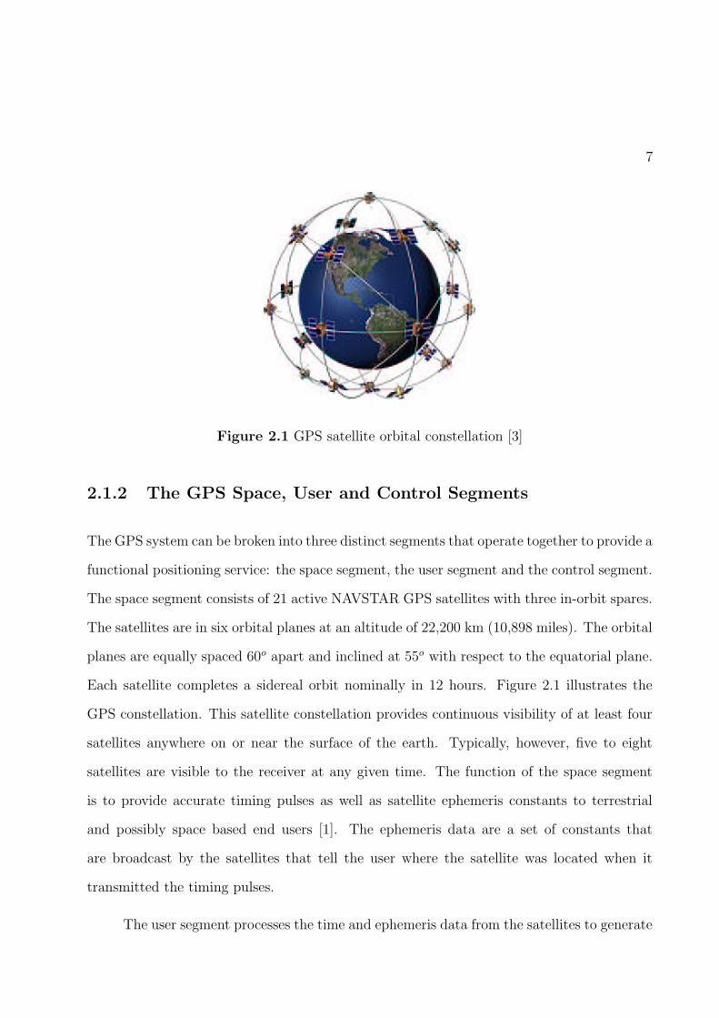
Figure 2.1 GPS satellite orbital constellation [3]

2.1.2 The GPS Space, User and Control Segments

The GPS system can be broken into three distinct segments that operate together to provide a

functional positioning service: the space segment, the user segment and the control segment.

The space segment consists of 21 active NAVSTAR GPS satellites with three in-orbit spares.

The satellites are in six orbital planes at an altitude of 22,200 km (10,898 miles). The orbital

planes are equally spaced 60o apart and inclined at 55o with respect to the equatorial plane.

Each satellite completes a sidereal orbit nominally in 12 hours. Figure 2.1 illustrates the

GPS constellation. This satellite constellation provides continuous visibility of at least four

satellites anywhere on or near the surface of the earth. Typically, however, five to eight

satellites are visible to the receiver at any given time. The function of the space segment

is to provide accurate timing pulses as well as satellite ephemeris constants to terrestrial

and possibly space based end users [1]. The ephemeris data are a set of constants that

are broadcast by the satellites that tell the user where the satellite was located when it

transmitted the timing pulses.

The user segment processes the time and ephemeris data from the satellites to generate

8

accurate position, velocity and timing estimates. Four satellites are required to compute the

four dimensions of position (x, y, z) and time. The user segment is typically broken into

three components: the antenna, the processor and the display. The antenna is tasked with

receiving the signal from the satellites. The processor then extracts data from the signals

and determines the navigation solution. Finally, the display component relays the navigation

solution to the end user or other instrument for further processing.

The control segment consists of a system of tracking stations located around the world.

The purpose of the control segment is to track the GPS satellites and furnish periodic updates

of their position drift and clock skew. These updates then allow the individual satellites

to adjust the ephemeris data that is provided to the user segment. The satellite update

information is actually provided to the control segment by each of the individual satellites

since the satellites are constantly monitoring their own position. The control segment then

inverts the data sent from each satellite and computes the navigation solution to construct

the new satellite positioning information.

2.1.3 The GPS Coded Data

The GPS code consists of three binary codes that shift the L1 and/or L2 carrier phase. The

C/A code (Coarse Acquisition) modulates the L1 carrier phase and is a repeating 1 MHz

Pseudo Random Noise (PRN) Code. This noise-like code modulates the L1 carrier signal,

“spreading” the spectrum over a 1 MHz bandwidth. The C/A code repeats every 1023

bits (one millisecond). There is a different C/A code PRN for each active satellite. GPS

satellites are identified by their PRN number which is the unique identifier for each pseudo-

random-noise code. The user terminal receiver then employs code-division multiple access to

distinguish between the different satellites. The C/A code that modulates the L1 carrier is

the basis for civilian location and navigation [2]. The P-Code (Precise) modulates both the

9

L1 and L2 carrier phases. The P-Code is a very long 10 MHz PRN code that repeats every

seven days. In the Anti-Spoofing (AS) mode of operation, the P-Code is encrypted into

the what is called the Y-Code. The encrypted Y-Code requires a classified AS Module for

each receiver channel and is for use only by authorized users with cryptographic keys. The

P (Y)-Code is the basis for the military precise positioning service (PPS). The Navigation

Message also modulates the L1-C/A code signal. The Navigation Message is a 50 Hz signal

consisting of data bits that describe the GPS satellite orbits, clock corrections, and other

system parameters [2].

2.1.4 The GPS Signal

The signal transmitted from the GPS spacecraft is right-hand circular polarized. Circular

polarization is used to avoid Faraday rotation problems associated with L-band propagation

through the earth’s ionosphere. Circular polarization has the additional benefit of not re-

quiring rotational alignment of a circularly polarized antenna at the user terminal. In order

to receive the maximum available power of right-hand circular polarized signals from the

satellites, the user terminal antenna must also be RHCP. A user terminal that is linearly

polarized will suffer a 3 dB loss in received power.

One common measurement for the quality of circular polarization is axial ratio. A

general elliptically polarized wave can be quantified by the magnitudes of its major and

minor axes of rotation. Axial ratio, AR, is simply the ratio of the major axis to the minor

axis and is typically stated in dB. AR provides a convenient measure for the deviation of a

general elliptically polarized wave from pure circular polarization. A pure circularly polarized

wave has and axial ratio of 0 dB. The axial ratio for acceptable circular polarization is often

specified to be at least 2 dB [4].

10

Table 2.1 GPS user terminal antenna electrical characteristics

Parameter Specification

Frequency L1 1575.42 ±2 MHz minimum, ±10 MHz desiredGain 4 dBicPolarization right hand circular polarizationAxial Ratio 3 dB or better nominalInput Impedance 50 Ω

The L1 band center frequency for civilian GPS applications is 1,575.42 MHz with the

C/A code requiring ±2 MHz of bandwidth. Additionally, impending government dereg-

ulation of the GPS system by 2006 are poised to make civilian use even more accurate.

Therefore, it is desirable to operate the L1 band with a bandwidth of ±10 MHz to take ad-

vantage of the encrypted P code and also to operate at the L2 band (1227.60 MHz). Thus,

antenna frequency coverage must either be continuous for L1 and L2 or dual banded covering

each band. Table 2.1 lists the GPS systems electrical characteristics.

The power density of the GPS signal arriving at the user terminal is at an extremely

low level. Typical power densities of less than -160 dBW are received. Therefore, reasonably

efficient user terminal antennas are necessary to take full advantage of the available power.

2.2 Cellular Radio

Conventional trunked radio comprises the systems where only one or a small number of

channels is available for use. Historically, radio communication were accomplished by placing

one large base station with a high power transmitter in or near the center of the desired

coverage area. This facilitates a very simple implementation but it means that the available

number of users communicating at one time is extremely limited. The cellular topology

11

breaks a large coverage market into a large number of small adjacent coverage “cells”. The

cells use smaller low power transmitters to serve only a portion of the mobile phone customers

at any given time. This type of system permits frequency reuse within the total coverage

area but not necessarily among adjacent cells. The channels are only reused when there is

enough distance between cells operating on the same frequency to ensure there will be no

interference. The result of this frequency reuse is a considerable increase in the total number

of users the system can handle.

2.2.1 History of Cellular Telephone

The first publicly available mobile telephone system was introduced by AT&T and South-

western Bell to Saint Louis, Missouri in 1946. The original system eventually spread to 25

cities with a single transmitter for each market. The half-duplex system operated at 150 MHz

with a 120 kHz RF channel bandwidth and could cover distances in excess of 30 miles [5].

The early system originally operated on six channels but considerable cross-channel interfer-

ence forced a reduction to three channels [6]. In the the 1950s, the channel bandwidth was

reduced to 60 kHz and then finally reduced to 30 kHz. Additionally, automatic trunking and

full-duplex transmission were introduced and the system was called IMTS, Improved Mobile

Telephone Service. The service limitations of IMTS were quickly realized and by 1976 there

were only 12 channels available to serve 543 paying customers in New York City which had

a market of around 10 million people [5].

The concept of the cellular phone system was introduced to the FCC in 1968 by AT&T.

The precursors to the current North American analog cellular phone system were developed in

the late 1970s to early 1980s. In July, 1978 Advanced Mobile Phone Service or AMPS started

operating in North America. Analog based cellular telephone service was first deployed at

AT&T labs in Newark, New Jersey, and in trials around Chicago, Illinois Bell. The Chicago

12

system was comprised of ten cells covering 21,000 square miles [7]. AMPS was eventually

approved by the FCC in 1983 and was the first standardized cellular service and is still

the most popular. The FCC originally allocated 666 channels using 40 MHz of bandwidth.

AMPS operates in the 824-894 MHz band with a 30 kHz channel bandwidth. In 1989 the

FCC allocated an additional 166 channels to the AMPS system to bring it to its spectrum

to the current specification of 70 MHz. Multiple customer access is accomplished through

FDMA (frequency division multiple access) and was designed in particular for urbanized

areas [8]. The 70 MHz band is broken into two halves of 1023 channels each. The forward

channel is 869-894 MHz and the reverse channel is 824-849 MHz. One channel from each

half of a full duplex communication link between the base station and the user terminal.

To overcome the low calling capacity of AMPS, Narrowband Analog Mobile Phone Service

(NAMPS) was developed. NAMPS uses a 30 kHz AMPS channel with frequency division

to obtain three 10 kHz sub-channels. Table 2.2 lists the major mobile radio standards for

North America.

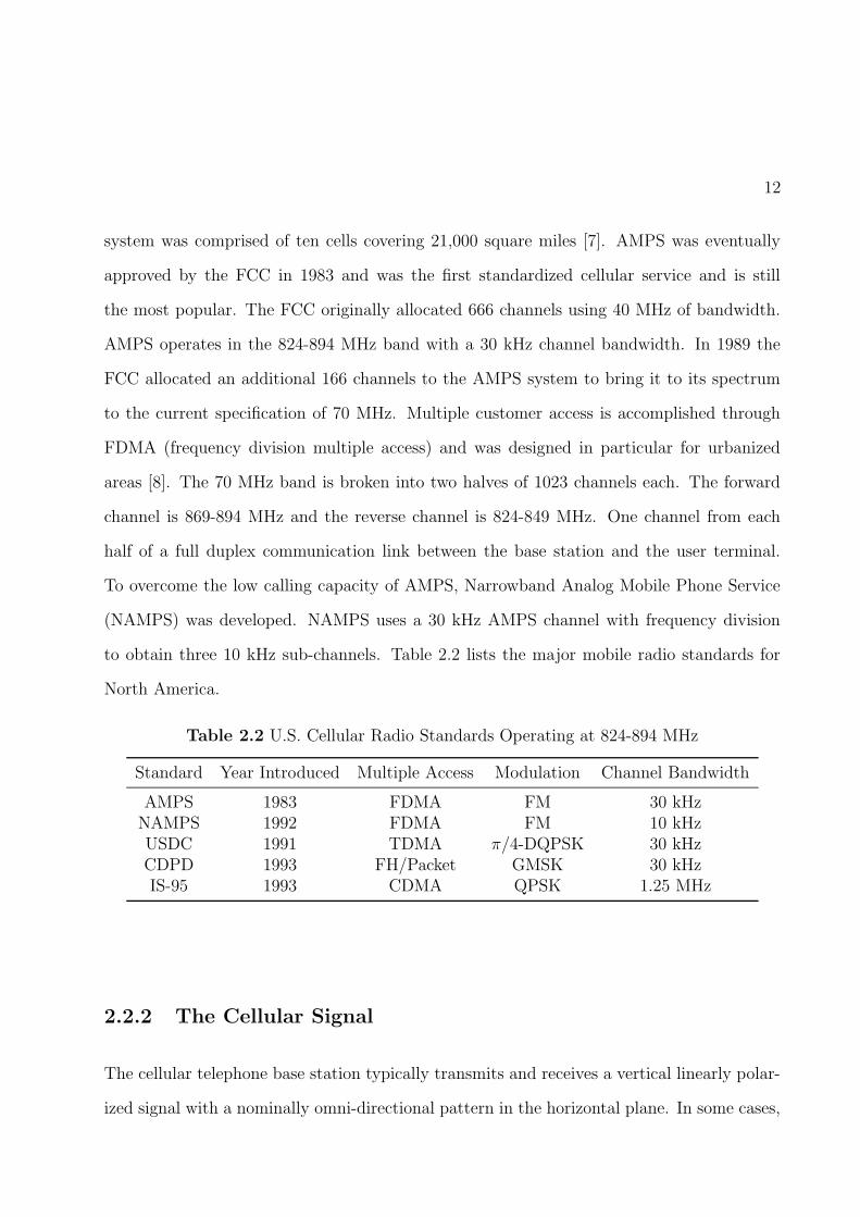
Table 2.2 U.S. Cellular Radio Standards Operating at 824-894 MHz

Standard Year Introduced Multiple Access Modulation Channel Bandwidth

AMPS 1983 FDMA FM 30 kHzNAMPS 1992 FDMA FM 10 kHzUSDC 1991 TDMA π/4-DQPSK 30 kHzCDPD 1993 FH/Packet GMSK 30 kHzIS-95 1993 CDMA QPSK 1.25 MHz

2.2.2 The Cellular Signal

The cellular telephone base station typically transmits and receives a vertical linearly polar-

ized signal with a nominally omni-directional pattern in the horizontal plane. In some cases,

13

Figure 2.2 Cellular nominal radiation pattern for user terminal

base stations use dual ±45 linear polarization for polarization diversity. Consequently, the

user terminal will also require vertical linear polarization to receive the maximum available

power. The 824-894 MHz cellular band is centered at 859 MHz with a bandwidth of 70 MHz

(8.2%). Input impedance of cellular antennas are universally specified to be 50 Ω. Table 2.3

lists the cellular system electrical characteristics.

Table 2.3 Cellular user terminal antenna electrical characteristics

Parameter Specification

Transmit and receive 824-894 MHzGain 3 dBiPolarization Vertical linearInput Impedance 50 Ω

2.3 The Return Link–A Case for a Combined GPS and

Cellular Terminal

The difficulty with GPS is that there is no return link. That is, a GPS terminal determines

its position, but that position is known only to the terminal user. The next wide scale

technology area for GPS is the integration of GPS with some type of wireless service to

provide communication of the GPS - derived position as well as messaging. One of the most

14

popular uses for this service is tracking of mobile cargo. For example, a railroad car with a

perishable cargo could report its position and status on a regular basis. If the refrigeration

unit fails, it can send a distress message along with its position. Additionally, in 1994

the FCC adopted its Enhanced 911 standards that might require the integrating of GPS

capabilities into cell phones [10].

There are four possible wireless services that can be integrated with GPS: Cellemetry,

cellular digital packet data or CDPD, two-way paging, and PCS. Cellemetry is a two-way

data communication platform that utilizes the non-voice or “control” channels of the AMPS

cellular system. Cellemetry uses the 42 AMPS control channels to transmit telemetric mes-

sages [11]. CDPD is a service that uses a full 30 kHz AMPS channel to transmit mobile

packet data. CDPD directly overlays on an existing cellular network and utilizes unused

bandwidth. A variety of different two-way paging systems currently exist. In the US, the

forward channel is 930-931 MHz and the reverse channel is 901-902 MHz. The data rate in

two-way paging is considerably lower than typical cellular based options [12]. In the US,

two types of PCS service bands exist: narrowband and broadband. PCS narrowband uses

900 MHz frequencies for many advanced paging services. Broadband PCS uses 1.9 GHz

frequencies for voice, data, and video services.

A GPS/Cellular antenna has been selected as a point design for a number of reasons.

The general cellular system offers nearly total wireless coverage within the US. Cellemetry

and CDPD are both within the standard cellular band. Selecting cellular leaves both of

those options open. Similar design concepts can be applied to other services such as PCS as

well. The antenna design will be limited to non-handheld portable Cellular operation. This

restriction ensures that the antenna will maintain correct orientation during operation. This

also allows the Cellular antenna to transmit at the maximum FCC limit of 3 Watts.

15

GPS Satellites

GPS Radiation Pattern

Cellular Radiation Pattern

Cellular Tower

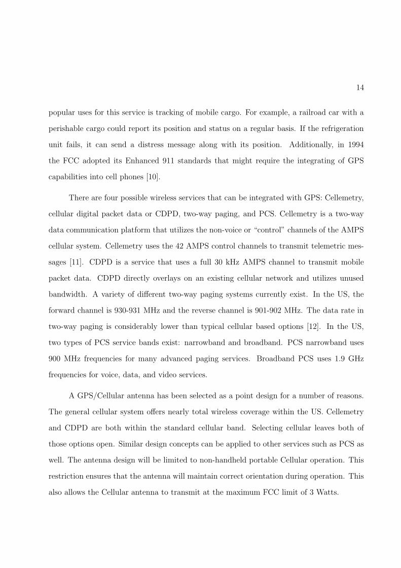
Figure 2.3 GPS and cellular user terminal radiation patterns

References

[1] T. Logsdon, The NAVSTAR Global Positioning System. New York: Van NostrandReinhold, 1992.

[2] B. Hofmann-Wellenhof, H. Lichtenegger, and J. Collins, GPS: Theory and Practice.New York: SpringerWien, 4 ed., 1997.

[3] M. E. Reece, “Global positioning system,” tech. rep., New Mexico Institute of Miningand Technology, http://www.nmt.edu/ mreece/gps/cover.html, 2000.

[4] R. B. Langley, “A primer on gps antennas,” GPS World, pp. 50–54, July 1998.

[5] T. S. Rappaport, Wireless Communications: Principles and Practice. New Jersey:Prentice Hall PTR, 1996.

[6] A. Peterson, Vehicle Radiotelephony Becomes a Bell System Practice. Bell LaboratoriesRecord, April 1947.

[7] F. H. Blecher, “Advanced mobile phone service,” IEEE Transactions on Vehicle Com-

munications, vol. VT-29, May 1980.

[8] The International Engineering Consortium, http://www.iec.org, Cellular Communi-

cations, 2001.

[9] K. Fujimoto and J. James, eds., Mobile Antenna Systems Handbook. Boston: ArtechHouse Publishers, 2nd ed., 2001.

[10] G. Miller, “Adding GPS applications to an existing design,” RF Design, pp. 50–57,March 1998.

[11] “Cellemetry data service via cellular,” tech. rep., Numerex Corp.,http://www.celemetry.org, October 2000.

[12] S. Tabbane, “Comparing one-way and two-way paging systems,” in Vehicular Technol-

ogy Conference,VTC 1999 - Fall. IEEE VTS 50th, vol. 4, pp. 2138–2142, September1999.

16

Chapter 3

The Cellular Antenna

This chapter presents the design process for the cellular portion of the combined GPS/cellular

antenna. Section 3.1 describes the points critical to the selection of a suitable antenna for

the cellular portion of the combined unit. Section 3.2 looks at several alternative antennas

that were investigated as possible candidate antennas. Section 3.3 investigates the effects of

operating with a finite size ground plane. Finally, Section 3.4 presents the recommendations

for final antenna designs.

3.1 Design Considerations

Design considerations start with the cellular antenna for a number of reasons. The operating

frequency of the cellular band is the lower of the two antennas and thus determines the

overall size of the unit. The direction of interest for the cellular signals is predominantly

in the horizontal plane and the direction of interest for the GPS signals is in the vertical

direction (eg. skyward). It follows naturally that the GPS antenna should be positioned

above the cellular antenna to prevent the cellular antenna from obstructing the field of view

17

18

Table 3.1 Cellular User Terminal Antenna Design Performance Goals

Parameter Specification

Transmit and receive 824-894 MHzGain 3 dBiPolarization Vertical linearInput Impedance 50 ΩPhysical Size Diameter < 4 inches (10 cm)

Height < 2 inches (5 cm)

of the GPS antenna. After a cellular antenna design is determined, the GPS antenna will be

designed and integrated with it. However, the search for the cellular antenna is conducted

with awareness that it must accommodate a GPS antenna.

Table 3.1 lists the desired design specifications. The initial factor that determines the

size of the antenna is the desired frequency of operation. The cellular band is 824–894 MHz,

giving a center frequency of 859 MHz and 8.1% bandwidth. The frequency of 859 MHz

corresponds to a wavelength of 35 cm. As a reference antenna, the half-wave dipole at this

frequency is 18 cm (7 inches) in linear extent. The desired size specified for the combined

unit is less than 4 inches (10 cm) in diameter and less than 2 inches (5 cm) tall. Thus, the

design challenge is find a cellular antenna that is considerably smaller than a conventional

dipole. The gain of the half-wave dipole is 2.15 dB[1]. It would be desirable to have at least

as much gain as a dipole. Therefore, the nominal gain is specified to be 3 dB. Linear vertical

polarization is necessary because the base station antennas are linear vertically polarized.

19

3.2 Candidate Antennas

The 4-inch diameter restriction presents a design challenge because this size is 0.29 wave-

length at 859 MHz since 4 inches is 10.19 cm and the wavelength is 34.9 cm. This is not

extremely small electrically; however, to also achieve the 8% bandwidth eliminates many

conventional approaches. Historically, the quarter-wave whip monopole has been the most

predominant antenna for handheld communication. It was determined that inductive load-

ing could be used to decrease the size of the λ/4 whip to 4–15% of a wavelength [2]. The

normal mode helix is the common form for a λ/4 whip with distributive inductive loading.

The λ/4 whip and inductively loaded monopoles are not considered as candidates for this

application because the majority of their physical extent lies in the vertical direction. The

desired radiation for the cellular band is in the horizontal plane and this type of antenna must

be oriented with the radiating element in the vertical direction for that mode of operation.

This orientation does not lend itself to attaching a GPS antenna.

Microstrip patches are popular antennas because of their low profile. Various types

of low-profile elements have recently been developed and they are fairly efficient radiators

that can be easily manufactured at low cost. The conventional microstrip patch is not a

candidate for the cellular portion because it produces a beam in the vertical direction rather

than horizontal. Therefore, more unusual approaches must be examined for reduced size

operation.

Techniques for size reduction include dielectric loading to reduce the electrical size, top

hat loading, and use of shorting pins or plates. Dielectric loading usually is accompanied

by bandwidth reduction and increased cost, so it is not a likely approach. Thus, we will

investigate antennas with top hat loading and shorting pins or plates, either separately or

in combination.

20

Table 3.2 Cellular user terminal candidate antennas

Candidate Size Envelope (wavelengths) Bandwidth (%)

Inverted-L λ/4 <1Inverted-F λ/4 2Dual inverted-F λ/4 5-7Planar inverted-F < λ/4 >8Meandering PIFA < λ/4 2-8

3.2.1 The Inverted-F Antenna

The inverted-F (IFA) family of antennas present a popular alternative for low profile omni-

directional applications. Wire forms of the IFA were extensively studied with computer

simulation and measurements at Virginia Tech [3]. The inverted-F antennas are variations

on the simple inverted-L antenna.

The inverted-L antenna is an end-fed short monopole with a horizontal wire element

placed on top that acts as a capacitive load. Figure 3.1 shows the physical layout of the

inverted-L antenna. The inverted-L antenna is an attractive alternative because of its simple

layout. The design is uncomplicated and can be easily manufactured with low cost materials.

Additionally, many of the electrical characteristics of the inverted-L are similar to those of

the well understood short monopole.

The radiation pattern of the inverted-L is nearly identical to that of the short monopole.

A z-directed short monopole produces a pattern that is omnidirectional and maximum in the

azimuth (x−y) plane and has nulls at θ = 0o, 180o (along the z-axis). The inverted-L oriented

with its radiating element in the z direction will also have a pattern that is omnidirectional

in the azimuth plane. The inverted-L however has an additional Eθ component due to the

horizontal arm [3]. The non-zero currents along the horizontal arm causes the radiation

pattern in the azimuth plane to deviate slightly from omnidirectional. The input impedance

21

L

H

Feed Point Ground Plane

Inverted-L

Z

X

Figure 3.1 Inverted-L antenna geometry

of the inverted-L is similar to that of the short monopole: low resistance and high reactance.

Low order approximations for the input resistance and reactance of the inverted-L are [4]:

RILA = 40

(

2π

λh

)2 (

1 − h

2(h+ L)

)2

(3.1)

XILA =−60h

(

2 − hh+L

)

(h+ L)2k

[

log

√3h

a− 1

3− 20a

9h(3.2)

+LaT − h/4

√

L2a + h2/4

+LaT/3 − 3h/4√

L2a + 9h2/4

]

where L is the length of the horizontal loading section, h is the height of the radiating section,

a is the radius of the antenna, k is the wave number (2π/λ), La = L + a and T = 1 − a/h.

Complete closed form derivations for both the input resistance and reactance can be found

in [4]. Equations (3.1) and (3.2) are plotted in Figure 3.2. As can be seen from Figure 3.2,

the relatively low resistance and high reactance for useful antenna dimensions make the

inverted-L difficult to impedance match to typical feedlines [3].

The inverted-F is a variation on the inverted-L that modifies the input impedance to be

nearly resistive and thus provides reduced mismatch loss. The inverted-F antenna is known

as a “shunt-driven inverted-L antenna-transmission line with an open end” as described by

King [5]. Figure 3.3 shows the layout of the the inverted-F antenna. The inverted-F adds

22

0 0.2 0.4 0.6 0.81

1.2

1.4

1.6

1.8

2

2.2

2.4

2.6

2.8

3

Normalized Loading Length (kL)

Res

ista

nce,

Ohm

s

a/h=0.01a/h=0.1

0 0.2 0.4 0.6 0.8100

200

300

400

500

600

700

800

Normalized Loading Length (kL)

Rea

ctan

ce, −

1 *

Ohm

s

a/h=0.01a/h=0.1

Figure 3.2 Inverted-L antenna input resistance and reactance from (3.1) and (3.2).

L

H S

Feed Point Ground Plane

Figure 3.3 Inverted-F antenna geometry.

23

800 810 820 830 840 850 860 870 880 890 9001

1.5

2

2.5

3

3.5

4

4.5

5

Frequency (MHz)

VS

WR

Figure 3.4 Inverted-F calculated input voltage standing wave ratio.

a second inverted-L section to the end of an inverted-L antenna. This additional inverted-

L segment adds a convenient tuning option to the original inverted-L antenna and greatly

increases the antenna usability. The location of the feedpoint, S, along the length of the

upper element provides the impedance tuning mechanism. The input impedance behavior

of the inverted-F antenna is similar to that of a transmission line antenna of length (H +L)

with its feed located at the tap point S [3]. Figure 3.4 shows the voltage standing wave

ratio for a typical inverted-F antenna operating at the cellular band. The antenna has the

dimensions H = 2.28 cm, L = 7.2 cm, S = 0.68 cm and was calculated with NEC2 using

a wire radius of 0.15 cm. The impedance match is improved considerably compared to the

standard inverted-L antenna. As can be seen from Figure 3.4, a VSWR of 2:1 is realizable

at the midpoint of the cellular band. The impedance bandwidth of this antenna is 1.5%.

Despite its relatively simple design, the design of an optimal IFA is not unique. Vari-

ations in the height of the radiator, the length of the horizontal element as well as the tap

point all impact the electrical performance characteristics of the IFA. Consequently, the de-

24

sign presented is not necessarily optimal; however, it does present the important aspects of

the inverted-F antenna performance. Further improvements to the input impedance match-

ing are possible by additional modification of the antenna geometry.

One critical problem that both the inverted-F and L antennas share with the short

monopole is very low impedance bandwidth. A typical wire inverted-F has about 2% band-

width [3]. Several modifications to the inverted-F have been examined that increase the

bandwidth of the antenna. One such variation is shown in Figure 3.5, the dual inverted-F

(DIFA). The dual inverted-F uses a parasitic inverted-L antenna placed next to the inverted-

Parasitic Element

Driven Element

Figure 3.5 Dual inverted-F antenna geometry.

F. The parasitic element has a length that is equal or nearly equal to L on the inverted-F.

Impedance bandwidths of nearly 4% have been achieved with the dual inverted-F [6].

The bandwidths of the inverted-L and F as well as the dual inverted-F are too small

for the cellular application. Additionally, the antenna horizontal extent of about 0.25 λo (3.4

inches) is rather large for a low-profile application. Thus, we dismiss the wire variations of

the inverted-F family.

3.2.2 The Planar Inverted-F Antenna

The planar version of the inverted-F antenna, the planar inverted-F antenna (PIFA), meets

the specifications which are required in a reduced size environment. The PIFA can be con-

25

Feed Point

Planar element Ground plane

Shorting Strap

Feed line

Figure 3.6 Basic layout of the planar inverted-F antenna.

sidered a direct extension of the inverted-F antenna that has the horizontal wire radiating

element replaced by a plate to increase its usable bandwidth. Figure 3.6 shows the general

structure of the planar inverted-F antenna. The compact size of the PIFA makes it a suitable

candidate. This unobtrusive design makes it ideally suited for mobile and handheld situa-

tions and complies with our low profile design goal. Accidental damage to the antenna via

unintentional contact with other objects is avoided. A flush mounted PIFA extends in height

approximately 1/20 of a wavelength as opposed to a conventional 1/4 wavelength monopole.

Additionally, the PIFA offers very high radiation efficiency and sufficient bandwidth in a

compact antenna. A bandwidth of 10% can be realized with the PIFA.

The increased complexity of the PIFA structure over the ILA, IFA and DIFA brings

an associated increase in complexity of the PIFA design and analysis. The size and aspect

ratio of the top radiating plate, the height of the plate above the ground plane, the size and

position of the ground strap and the feed point location all have considerable impact on the

electrical performance of the antenna.

The size of the PIFA radiating top plate can be calculated approximately using [7]:

λcenter = 4(L+W ) (3.3)

26

where L and W are respectively the length and width of the plate. The resonant frequency

is also influenced by the aspect ratio of the top plate (W/L). The width of the grounding

strap, S, in relation to the width of the radiating top plate is also particularly important in

determining the radiating behavior of the PIFA. Figure 3.7 [8] shows how the current flow on

the surface of the top plate varies with different top plate and grounding strap configurations.

In general, a greater top plate aspect ratio will result in a lower the resonant frequency for a

given grounding strap width. For an aspect ratio of W/L > 1, there is an inflection point in

the resonant frequency when W −S = L and the resonant frequency begins to increase with

increasing aspect ratio. As seen in Figure 3.7, the current on the planar element generally

flows to the open-circuit edge on the long side of the top plate when W − S < L. When

W−S > L, the current flows to the open circuit edge along the short side of the top plate [8].

The inflection point in the resonant frequency is attributed to this change in current flow.

The inflection point can be seen clearly in the case of W = L and where S << W , the

current flows almost equally along the both the W and L dimensions.

Like the resonant frequency of the PIFA, the relative impedance bandwidth is affected

by the design of the structure. The height of the radiating top plate, H, and the width of

the grounding strap have the greatest influence on the bandwidth of the PIFA. In general,

the bandwidth increases with increasing top plate height. However, as the height of the

top plate approaches the magnitude of L = W , the height begins to influence the resonant

frequency. When the grounding strap width is very small, S << W , the resonant frequency

is given by:

λcenter = 4(L+W +H) (3.4)

The width of the grounding strap similarly affects the bandwidth. The limiting case, where

the grounding strap is the same width as the top plate, the bandwidth of the PIFA is

greatest. This case corresponds to the operation of a short circuited microstrip antenna.

27

L

W L / W = 0.5

L / W = 1.0

L / W = 2.0

S = W W / 2 < S < W S << W

Shorting Plate

Figure 3.7 Surface current on PIFA top plate for various top plate aspect ratios and ground-

ing strap widths.

This PIFA with a W/L = 2.0 and H/λ0 = 0.053 has a relative bandwidth of 10% [8]. As

the width of the grounding strap decreases, the relative bandwidth of the PIFA decreases.

The bandwidth of a PIFA with the grounding strap width much less than the width of the

top plate (S/W ≤ 0.1) can be reduced to below 1%.

There are several procedures available for designing PIFAs and many different PIFA

layouts may satisfy the same design criteria. An excellent overview of how the design vari-

ables affect the electrical operation of the PIFA is given in [8]. One particular design of a

cellular PIFA is given by [9] and is re-analyzed here for clarity. The design of Figure 3.8 has

a radiating top plate that is 6.40 cm long and 2.29 cm wide. The height of the top plate is

1.78 cm and the shorting strap is equal in width to the top plate. The metal strips used in

the simulation are 60 mils thick and the probe feed is model as a single strip 1.6 mm wide.

The antenna is simulated over and infinite ground plane with a moment method code.

28

6.40 cm

1.78 cm

2.59 cm 2.29 cm

1.78 cm

Figure 3.8 Typical PIFA designed for operation near cellular band.

The PIFA of Figure 3.8 shows and excellent impedance match to 50 Ω at 1 GHz.

Although slightly higher than 900 MHz, the center frequency can be easily adjusted and the

antenna retuned to operate closer to the cellular band with only minor geometry scaling.

The 2 : 1 VSWR bandwidth in Figure 3.9 shows that this PIFA geometry can easily cover

the 8% bandwidth requirement for the cellular signal.

Several further modifications to the conventional PIFA have been studied and shown to

operate favorably in the cellular band. One particular modification is a PIFA with a partial

shorting plate. This shorted PIFA was designed for operation on a handset was demonstrated

to have 8 to 12% bandwidth [10]. This antenna, however, has an appreciable amount of

radiation in the broadside direction as well as the horizontal plane. Considering the fact

that the GPS antenna is to be placed above the cellular antenna, the design should minimize

the cellular radiation in the broadside (vertical) direction. Therefore this modification of the

29

0.95 1 1.05 1.1 1.15 1.21

1.5

2

2.5

3

3.5

4

4.5

5

Frequency (GHz)

VS

WR

Figure 3.9 VSWR versus frequency for the PIFA of Figure 3.8 calculated using moment

method code.

0 .2 .5 1 2 5 inf

.2

.2

.5

.5

1

1

2

2

Figure 3.10 Input reflection coefficient for the PIFA of Figure 3.8 calculated calculated

using moment method code

30

conventional PIFA is not considered as a candidate antenna.

3.2.3 The Meander Planar Inverted-F Antenna

One other variation of the PIFA presented in [11], has a further reduction in size while still

maintaining adequate bandwidth. The meander PIFA is capable of 10% bandwidth and is

only an eighth of a wavelength long. Figure 3.11 shows the meander PIFA as a modification

of the conventional PIFA design that is slightly reduced in size from the conventional PIFA.

It uses several slits cut laterally in the PIFA radiating element. These slits effectively act to

increase the electrical length of the antenna and allow for reduced overall antenna volume.

As was shown in Subsection 3.2.2, the height of the radiating element greatly influences the

impedance bandwidth of the antenna. The meander PIFA of [11] achieves a reduced height

by incorporating a chip resistor in place of the conventional grounding strap or shorting pin.

L

W/2

W

l S

L/4 L/4

B

A

h

Feed Point

Shorting Resistor

Ground Plane

d

Figure 3.11 Meandering planar inverted-F antenna layout

The geometry studied by Wong is shown in Figure 3.11 with the following dimensions:

L = 40 mm, W = 25 mm, l = 20 mm, h = 3.2 mm and S = 2 mm. The feed is located with

31

Table 3.3 Meander PIFA of [11] with various loading resistances

Resistance, Ω f0, MHz d/AB BW , %

0 872 0.06 0.62.2 871 0.25 3.43.3 861 0.35 4.74.7 860 0.5 6.85.6 857 0.6 8.66.8 857 0.7 11.2

Simple PIFA 1298 0.06 0.9

length d along the line AB. This modified PIFA design produces an antenna with a length

< λo/8 and a height of 0.01λo. Table 3.3 [11] shows the impedance bandwidth and center

frequency achieved by the meander PIFA for various loading resistances. A conventional

PIFA is included in the table for comparison. It can be seen that for increasing loading

resistance, the corresponding impedance bandwidth is increased. A maximum bandwidth of

11.9% is achieved when a 6.8 Ω resistor is used.

The increase in impedance bandwidth due to the loading resistor comes at the expense

of radiation efficiency. Considerable ohmic losses are experienced when the loading resistor is

in place and consequently a reduction in antenna gain is observed. Reference [11] estimates

that there is a 6 dB reduction in antenna gain when the 5.6 Ω resistor is used. The diminished

gain severely limits our ability to implement this design into our antenna into our final design

due to the fact that antenna gain is a key performance characteristic.

3.3 Ground Plane Effects

The candidate antennas discussed so far assume that a large ground plane is used. A detailed

study on the effects of operating the PIFA in a reduced ground plane environment is presented

32

in [12]. The size of the ground plane plays an important role in the behavior of the PIFA.

The resonant frequency, input impedance, bandwidth and gain are all impacted when the

PIFA is operated over a finite size ground plane.

The resonant frequency for a PIFA with a fixed top element and grounding strap

size tends to remain fairly constant for large ground plane sizes. As the ground plane size

is reduced, the value of the resonant frequency oscillates around the value for the infinite

ground plane case until the ground plane size reaches about 0.2λ in length. At that point,

the resonant frequency is highly dependent on the size of the ground plane and it increases

linearly with decreasing ground plane size.

The relative bandwidth of the PIFA increases with increasing ground plane size. As in

the center frequency case, the relative bandwidth oscillates around the value of the infinite

ground plane case. However, the PIFA relative bandwidth exhibits a stronger dependence

on ground plane size than the center frequency does for larger ground planes. It is reported

in [12] that a ground plane size of at least 0.8λ is required to achieve the desired 8% impedance

bandwidth of the Cellular band.

The gain of the PIFA is influenced by the size of the ground plane as well. The gain

of the PIFA increases with increasing ground plane size. It then reaches a local maximum

around 0.9λ and begins to oscillate to the infinite ground plane case of nearly 5 dB. To

achieve the desired 3 dB in gain for the Cellular band, a ground plane of at least 0.5λ is

required[12].

33

3.4 Recommendations

The initial investigation of the several different cellular antenna designs has lead to the

recommendation of one particular design. Based on the considerations and the critical

parameters necessary to the operation of the cellular portion of the antenna, the conventional

PIFA has been selected as the most suitable antenna for the cellular portion of the integrated

antenna. The design selected will be presented and analyzed in Chapter 5.

References

[1] W. L. Stutzman and G. A. Thiele, Antenna Theory and Design. New York: John Wiley& Sons, Inc., 1998.

[2] K. Fujimoto and J. James, eds., Mobile Antenna Systems Handbook, ch. 7 - Antennasand Humans in Personal Communications. Boston: Artech House, 2nd ed., 2001.

[3] A. Gobien, “Investigation of low profile antenna designs for use in hand-held radios,”Master’s thesis, Virginia Polytechnic Institute and State University, August 1997.

[4] A. D. Wunsch, “A closed-form expression for the driving-point impedance of the smallinverted L antenna,” IEEE Transaction on Antennas & Propagation, vol. 44, pp. 236–242, February 1996.

[5] R. W. P. King, J. C. W. Harrison, and D. H. Denton, “Transmission line missile anten-nas,” IRE Transactions on Antennas and Propagation, vol. 8, no. 1, pp. 88–90, 1960.

[6] H. Nakano, N. Ikeda, Y.-Y. Wu, R. Suzuki, H. Mimaki, and J. Yamauchi, “Realizationof dual-frequency and wide-band VSWR performances using normal-mode helical andinverted-f antennas,” IEEE Transaction on Antennas & Propagation, vol. 46, pp. 788–793, June 1998.

[7] Z. Liu, P. Hall, and D. Wake, “Dual-frequency planar inverted-F antenna,” IEEE Trans-

action on Antennas & Propagation, vol. 45, pp. 1451–1458, October 1997.

[8] T. Taga, Analysis, Design, and Measurement of Small and Low-Profile Antennas, ch. 5:Analysis of Planar Inverted-F Antennas and Antenna Design for Portable Radio Equip-ment. Boston: Artech House Publishers, 1992.

[9] Zeland Software Inc., IE3D User’s Manual, 8 ed., 2001.

[10] M. A. Jensen and Y. Rahmat-Samii, “Fdtd analysis of pifa diversity antennas on a hand-held transceiver unit,” in Antennas & Propagation Society International Symposium

Digest, vol. 2, (Ann Arbor, MI), IEEE, July 1993.

[11] K.-L. Wong and K.-P. Yang, “Modified planar inverted-F antenna,” Electronic Letters,vol. 34, pp. 7–8, January 1998.

34

35

[12] M.-C. T. Huynh, “A numerical and experimental investigation of planar inverted-Fantenns for wireless communication applications,” Master’s thesis, Virginia PolytechnicInstitute and State University, Blacksburg, VA 24060, October 2000.

Chapter 4

The GPS Antenna

This chapter presents the design process for the GPS portion of the combined GPS/cellular

antenna. Section 4.1 describes the points critical to the selection of a suitable antenna for

the GPS portion of the combined unit. Section 4.2 examines several alternative antennas

that were investigated as possible candidate antennas. Finally, Section 4.3 presents the

recommendations for final antenna designs.

4.1 Design Considerations

The basic design for the cellular portion of the integrated antenna was discussed in Chap-

ter 3. Here we consider the GPS portion of the integrated unit. The GPS antenna design

must consider the geometry of the cellular antenna. The reduced size of the cellular PIFA

determines the starting point for the size of the GPS antenna. The GPS design must take

into account the size of both the PIFA top radiating element and the PIFA ground plane as

well as the height of the radiating element above the ground plane. These two restrictions

are critical to the design of the GPS element for several reasons. The GPS antenna will

36

37

PSfrag replacements10 − 15

Figure 4.1 GPS nominal radiation pattern

be located on top of the cellular antenna and, thus, the cellular antenna will be effectively

acting as the ground plane for the GPS. Therefore the GPS antenna must be able to operate

over a ground plane that is comparatively small and possibly in proximity to a much larger

ground plane.

GPS signals are relatively weak compared to broadcast signals from terrestrial stations

and therefore antenna gain is an important factor. While it is common to include an on-

board LNA, typically with a gain of 26 dB, an antenna gain of at least 4 dBic is desirable in

order to deal with the low-power signals. The ideal radiation pattern of a terminal user GPS

antenna is shown in Figure 4.1. The pattern is a broadside unidirectional beam. Constant

coverage should be maintained in azimuth. To reduce the reception of multipath signals, it

is necessary that the antenna pattern have deep nulls along the horizontal [1]. Therefore, the

elevation pattern should be nearly constant down to an angle of 10 − 15 from horizontal.

Realistically though, the radiation pattern cannot achieve the discontinuity and the coverage

will gradually roll off with angle. The gain at the horizon should be reduced by at least 25

dB to ensure proper signal rejection. The nulls along the horizontal will serve an additional

38

function in respect to the integrated unit. The majority of the cellular signal is directed

along the horizontal and the nulls in the GPS pattern will aid in rejecting the cellular signal;

this can be important for controlling intermodulation effects.

Circular polarization is used on the GPS signal to avoid Faraday rotation problems

associated with L-band propagation through the earth’s ionosphere. It also has the additional

benefit of not requiring rotational alignment of the antenna at the user terminal. The signal

transmitted from the satellites is right-hand circular polarized and, therefore, the terminal

antenna must also use RHCP in order to have the maximum received signal strength. The

purity of the circular polarization has a direct impact on the receive gain of the antenna.

The higher the axial ratio of the antenna, the less efficient the antenna will be at receiving

the circularly polarized signal. The axial ratio of the antenna is specified to be at most 2 dB

over the entire bandwidth of the transmitted signal.

Circular polarization typically has the drawback of being slightly more difficult to

create than simple linear polarization in an antenna. A simple yet didactic example of

how circular polarization works and how to create it is the crossed dipole antenna. The

crossed dipole consists of two orthogonally crossed dipoles fed in phase quadrature. The

spatial rotation of the two antennas with the combination of the two feed signals 90 out of

phase produces the desired circular polarization. The difficulty with this and many similar

configurations is the need for two feed structures and complicated power combiners. Many

popular CP antennas use this two-feed method but for the design presented here it is desirable

to use only a single feed configuration.

39

Table 4.1 GPS user terminal antenna design performance goals

Parameter Specification

Frequency (L1) 1575.42 ±2 MHzGain 4 dBicPolarization right hand circular polarizationAxial Ratio 3 dB or better nominalInput Impedance 50 ΩPhysical Size Diameter < cellular PIFA top plate

Height < 0.5 inch (1.25 cm)

4.2 Candidates Antennas

Historically, several different types of antennas have been used in GPS receiving systems.

These antennas include monopole and dipole configurations, quadrifilar helices and mi-

crostrips. The type of antenna selected must conform to the reduce size requirements while

meeting the electrical performance characteristics. The reduced size requirement immedi-

ately eliminates the monopole and dipole configuration. A λ/4 monopole at the L1 band is

nearly 2 inches long–well larger than the 0.5 inch requirement.

4.2.1 The Qudrifilar Helix

There is considerable interest in helix antenna variations for use in GPS applications. The

quadrifilar helix is one of the most popular designs because of its relatively compact size

and its excellent circular polarization properties [2]. Quadrifilars with axial ratios of less

than 3 dB are common. One of the difficulties with the quadrifilar is its vertical extent.

An optimized design for a GPS quadrifilar is presented in [2] and it shows fractional turn

quadrifilars with axial lengths from 0.2λ to 0.35λ. This corresponds to antenna heights of

1.5 to 2.6 inches, which are considerably larger than our height requirement of less than 0.5

40

inch.

An additional problem typically associated with the quadrifilar helix is phase center

variation over the pattern. The radiating elements of the quadrifilar helix are on the perime-

ter of the antenna volume and the effective phase center of the antenna changes with the

view angle. It is desirable to have the antenna phase center remain constant over the entire

viewable region of the antenna in order to maintain measurement accuracy. This is diffi-

cult to achieve with an antenna that is spatially distributed such as the quadrifilar helix.

The limitations presented here show that the quadrifilar helix should not be considered as a

design for the integrated antenna.

4.2.2 The Rectangular Microstrip Patch

The elimination of the alternate antenna configurations leaves the microstrip variations as

the most suitable for the low profile application. Typical patch antennas can have gains as

high as 5 to 6 dB and 3-dB beamwidths of 70 to 90 [3]. The generic microstrip patch

antenna consists of a planar dielectric substrate material with of a radiating patch on one

side and a ground plane on the other. The radiating patch can be shaped in any number of

geometries depending on the desired electrical and radiation characteristics of the antenna.

The patch is fed against the ground at the appropriate point on or near the radiating patch

for desired operation. Common feed methods are the microstrip line, coaxial probe, and

proximity coupled feeds. The simplest microstrip patch antenna consists of a square or

rectangular radiator.

The rectangular microstrip patch antenna is the simplest geometry of the microstrip

patch antenna family. Figure 4.2 shows the generic layout of a rectangular microstrip an-

tenna. The radiating element has length L and width W . A charge distribution is developed

41

h

PSfrag replacements

L

W

εr

Figure 4.2 Basic rectangular microstrip patch antenna geometry

on the underside of the patch metalization and the ground plane when the patch is excited by

the feed. This particular patch antenna is shown with an edge fed microstrip feed. In order

to maintain real-valued input impedances, the microstrip patch antenna is normally operated

near resonance [4]. The substrate thickness h is typically much less than a wavelength.

The electrical behavior can be visualized as two magnetic surface currents flowing

along the radiating edges as seen in Figure 4.3. These magnetic currents are the result of

the fringing fields along the radiating edges. The additional length,∆l, added to the patch

due to the fringing fields is approximately the thickness of the substrate, h. An approximate

value for the length of a resonant half-wave patch is [4]

L ≈ 0.49λ√εr

(4.1)

where λ is the free-space wavelength and εr is the relative dielectric dielectric constant of

the media.

Equation (4.1) gives a basic first order approximate model for the resonant frequancy

of the rectangular microstrip patch antenna. Several other more complicated, more accurate

models have been studied and provide considerably more insight into the behavior of the

rectangular microstrip patch antenna. The cavity model is one of the frequently employed

methods for studying well defined structures such as the rectangular and other canonical

patch antenna geometries.

42

Equivalent magnetic currents, M s

Radiating Slots

PSfrag replacements

L

W

Radiating

Slots∆l ∼= h

Figure 4.3 Basic rectangular microstrip patch antenna

4.2.2.1 Cavity Model

The cavity model is an analytic approach which provides a reasonably accurate model of

the patch antenna because microstrip patch antennas narrow-band resonant nature. The

microstrip patch antenna can be thought of as a leaky or lossy cavity resonator. The patch

element is approximated as a closed cavity with magnetic side wall boundaries and electric

boundaries on the top and bottom. It ignores the open nature of the radiating antenna

structure but provides a model which can be solved analytically. The cavity model can be

used to determine the current distribution and radiation pattern of several different canonical

patch geometries.

The field distribution of the patch antenna can be divided into two distinct regions.

The interior fields are the fields inside the cavity and are used to determine the impedance

properties of the patch as well as the current distributions on the patch. The exterior fields

are outside the cavity and determine the radiation properties of the patch. The cavity

model makes the assumption that the dielectric layer is electrically thin, h << λ. From this

43

assumption several important observations can be made regarding the electrical behavior

of the patch. First, the fields in the interior region are not dependent on z, ∂/∂z ≡ 0.

Correspondingly then, the field distribution in this region is described by TMz modes with

∂/∂z ≡ 0. This leaves only three field components to solve for in the cavity: the normal

electric field Ez and the transverse magnetic fields Hx and Hy.

Beginning with Maxwell’s equations for the interior region of the patch we have

∇× ~E = −jωµ0~H (4.2)

∇× ~H = jωε ~E + ~J (4.3)

∇ · ~E = ρ/ε (4.4)

∇ · ~H = 0 (4.5)

The z-directed current from the source is assumed to be independent of z and thus ∇ · ~J =

0 = −jωρ, which then reduces Equation (4.4) to

∇ · ~E = 0 (4.6)

Equations (4.2), (4.3) and (4.6) can then be combined to give the familiar wave equation

∇×∇× ~E − k2 ~E = −jωµ0~J (4.7)

where k2 = ω2µ0ε0εr is the wavenumber in the dielectric. Since the feed source has been

specified to be z-directed only, we can rewrite Equation (4.7) as

(

∇2 + k2)

Ez = jωµ0Jz (4.8)

The left-hand side of Equation (4.8) can be broken into its components and can be rewritten

as

∂2Ez

∂x2+∂2Ez

∂y2+ k2Ez = jωµ0Jz (4.9)

44

Equations (4.8) and (4.9) show that the cavity model assumptions are consistent. The

electric boundary on the top of the patch is satisfied because the E-field is only a function

of z, ~E = Ez z. The magnetic wall boundary is satisfied because ∂Ez/∂z = 0.

The electric field for the patch antenna can be determined by solving Equation (4.8).

Let ψmn be the eigenfunction of the homogeneous wave equation (∇2 + k2)Ez = 0, and let

kmn be the eigenvalues of k. The eigenfunctions are assumed to be orthogonal and thus the

solution to Equation (4.8) has the form

Ez(x, y) =∑

m

∑

n

Amnψmn(x, y) (4.10)

where Amn are the amplitude coefficients corresponding to the electric field mode vectors.

The coefficients, Amn, are determined by the excitation current. By using the orthonormal

properties of the eigenfunctions they are specified as

Amn =jωµ0

k2 − k2mn

∫∫

feed

ψ∗

mnjzdxdy (4.11)

The resonant frequencies are then found by setting k2 − k2mn = 0 and are given by

fmn = kmnc/(2π√εr) (4.12)

with the wave number for the mode m,n being

k2

mn = (mπ/L)2 + (nπ/W )2 (4.13)

where m,n = 0, 1, 2 . . . and x, y are the dimensions along the length L and width W ,

respectively, of the patch. For the dominant TM10 mode of operation this then results in a

resonant frequency of

f =c

2L√εr

(4.14)

45

which is similar to our original approximate expression for the resonant frequency shown in

Equation (4.1). The resonant mode electric field in the cavity under the patch rectangular

is then given by [5]

Ez = Eo cos(mπx/L) cos(nπy/W ) (4.15)

It can be seen then from Equation (4.15) that for the dominant TM10 mode the electric field

varies sinusoidally along the length L of the patch and is constant along the width.

Equation (4.12) is based on the assumption that a perfect magnetic wall is present

at the edge of the radiating element and no fringing fields are present. The fringing fields

which are illustrated in Figure 4.4 can be accounted for using the empirical effective length

formulas [6]

Le = L+ h/2 (4.16)

We = W + h/2 (4.17)

A more accurate formula for resonant frequency is given in [5] which makes use of an effective

dielectric constant

fr1 = fr0εr

√

εe(L)εe(W )

1

1 + ∆(4.18)

where

∆ =h

L

[

0.882 +0.164(εr − 1)

ε2r+εr + 1

πεr0.758 + ln(L/h+ 1.88)

]

(4.19)

and the effective dielectric constant is given by

εe(α) =εr + 1

2+εr − 1

2

[

1 +10h

α

]

−1/2

(4.20)

with fr0 being the resonant frequency determined from Equation (4.12) and α is either the

length L or the width W . Figure 4.4 illustrates the electric field of the dominant TM10 mode

varying sinusoidally along the patch length and it includes the effects of the fringing fields

at the edge of the patch.

46

+ + + + + - - -

- -

++++++++ - - - - - - - -

PSfrag replacementsh

L

Figure 4.4 Rectangular microstrip patch antenna charge density and field distribution with

perimeter fringing fields

(a) Eθ for TM10 patch, φ = 0 (b) Eφ for TM10 patch, φ = 90

Figure 4.5 Radiation patterns for rectangular microstrip patch antennas calculated using

cavity model [5].

4.2.2.2 Radiation Characteristics

The rectangular microstrip patch antenna can be operated in several different modes. How-

ever, the most common modes of operation for the antenna are the TM10 and TM01 modes [6]

because they produce principal plane radiation patterns with maxima in the broadside di-

rection. Higher order modes tend to produce maxima off broadside. Figure 4.5 shows the

computed principal plane radiation patterns for the TM10 mode of two antennas calculated

with a cavity model [5]. The two antennas have dimensions W = 1.5 · L and dielectric

constants of εr = 2.32 and 9.8. The radiation patterns presented give broad beams with

47

maximums directed normal to the plane of the radiating element. The desired nulls along

the horizontal are achieved in the Eφ principal plane cut. Simple expressions exist which

approximate the radiation patterns for the rectangular patch antenna and are given by [4]

Eθ = E0 cosφf(θ, φ) (4.21)

Eφ = −E0 cos θ sinφf(θ, φ) (4.22)

with

f(θ, φ) =sin

(

βW2

sin θ sinφ)

βW2

sin θ sinφcos

(

βL

2sin θ cosφ

)

(4.23)

where β is the free-space propagation constant. These expressions again depend on the thin

substrate assumption and they neglect substrate and fringing effects. Further simplifications

can be made for the principal plane patterns as [4]

FE(θ) = cos

(

βL

2sin θ

)

(4.24)

FH(θ) = cos θsin

(

βW2

sin θ)

βW2

sin θ(4.25)

4.2.2.3 Input Impedance

The input impedance of a rectangular microstrip patch antenna can be determined by re-

turning to the cavity-model approximation for the fields in the patch. The input impedance

is given as

Zin =Vin

I0(4.26)

with Vin being the input voltage at the feed point and is computed as [3]

Vin = −jωµ0hI0

∞∑

m

∞∑

n=0

ψ2mn(xf , yf )

k2 − k2mn

Gmn (4.27)

48

which leaves the expression for the input impedance as [3]

Zin = −jωµ0h

∞∑

m

∞∑

n=0

ψ2mn(xf , yf )

k2 − k2mn

Gmn (4.28)

where

Gmn = sin c(nπDx/(2L)) sin c(mπDy/(2W )) (4.29)

where Dx ·Dy is the equivalent cross-sectional area of the feed point centered at (xf , yf ). The

losses in the dielectric constant can be accounted for by including an effective loss tangent

δeff factor in Equation (4.28). The expression for k2 can be modified as [3]

k2 = k2

0εr(1 − jδeff ) (4.30)

Equation (4.28) can then be evaluated for the dominant TM10 mode at k210 = k2

0εr which

leaves the input resistance as [3]

R10 =ωµ0h

k20εrδeff

2

LWcos2 (πxf/L) (4.31)

A slightly less complicated expression for impedance can be found in [4] and is given by

Rin = 90ε2r

εr − 1

(

L

W

)2

(4.32)

Equation (4.32) neglects the thickness of the substrate and is only appropriate for patches

fed from the edge. Equation (4.32) is the reduction of an expression presented in [7]. The

model is an approximation of the cavity model and considers dielectric effects as well as feed

location along the centerline.

Rin = 90er

pc1εrµr

(

L

W

)

sin2

(πxf

L

)

(4.33)

where the p factor is the ratio of the power radiated by the patch to that of a Hertzian dipole

and is given approximately by

p = 1 +a2

20(kW )2 + a4(3/560)(kW )4 + b2(1/10)(kL)2 (4.34)

49

with the polynomial coefficients of p being a2 = −0.16605, a4 = 0.00761 and b2 = −0.09142.

Additionally, the factor c1 is given by

c1 = 1 − 1

n2+

2/5

n4(4.35)

where n is the index of refraction for the medium, n =√εrµr. Also required in the calculation

is the radiation efficiency of a Hertzian dipole which is given by

er =P h

r

P hr + P h

SW

(4.36)

with the radiated (space-wave) power being approximately

P hr =

1

λ20

(kh)2[

80π2µ2

rc1]

(4.37)

and the surface-wave power being approximately

P hSW =

1

λ20

(kh)3

[

60π3µ3

r

(

1 − 1

n2

)3]

(4.38)

All of the expressions for input impedance require the dielectric substrate thickness be thin.

The value of the dielectric constant also plays a role in how well these approximations hold.

Typically, higher dielectric constants give less accurate approximations. Equation (4.33) is

accurate (within 2%) with εr = 2.2 for thickness h < 0.06λ0. However when εr is increased

to 10 the approximation only holds for thicknesses < 0.02λ0 [7].

4.2.2.4 Circularly Polarized Microstrip Antennas

Circular polarization can be produced by microstrip patch antennas in a variety of manners.

Typically, the methods for producing CP in a patch antenna are classified by the feed method

which excites CP radiation. Two broad categories are dual-feed methods and single-feed

methods. Dual-feed patches are fed at two points on the antenna and 90 out of phase. The

feeds are typically then combined either by a external 3dB power divider or a quarter-wave

50

x

a = b + c

b

y

2 3 4

1

(a) Nearly square

a

y

a a'

x 2 3

4

1

(b) Truncated corners

x

a

a

y

2 3 4

1

(c) Angled slot

Figure 4.6 Single feed method microstrip patches for circular polarization [8],[5].

offset feed [5]. Dual feed methods have the advantage of being conceptually easier to design

even though they require external components.

The single feed method is slightly more complicated to analyze and design than the

dual feed method. The antenna must excite two orthogonal modes with a single feed. This

is accomplished by carefully choosing the radiating patch geometry such that degenerate

modes are properly excited on the patch. These degenerate modes have equal or nearly

equal amplitudes and radiate in orthogonal directions to each other.

Figure 4.6 shows three different methods of creating circular polarization in a square

or nearly square patch with only one feed. The antenna in Figure 4.6(a) is a patch that has

one edge length slightly greater than the other, a > b. If c is small compared to b, c/b << 1

then the resonant mode numbers for the x-directed and the y-directed modes will be close

enough to assume that the effective loss tangent for each mode is identical [8]. Feeding

the antenna at either point 1 or 3 will excite the mode normal to that particular edge and

the antenna will behave as a linearly polarized microstrip patch antenna. However, if the

antenna is fed from either point 2 or 4 or along either patch bisecting diagonal, both of the

51

degenerate modes will be excited and circular polarization will be created. The position of

the feed along the diagonal has an impact on both the input impedance seen by the patch

and to a small extent the resonant frequency of operation.

The antenna in Figure 4.6(b) is a corner truncated square patch. Two opposing corners

are trimmed a small amount, ∆s. This antenna creates circular polarization in much the

same way as the antenna in Figure 4.6(a) does by creating two orthogonally degenerate

modes from the slight perturbation in antenna geometry due to the truncated corners [3].

In this case however, the antenna must be fed from point 1 or 3 or from some point along

either of the antenna center lines. Both right and left hand sense circular polarization may

be established with this geometry depending on which feed point is chosen. If the antenna

is fed along the diagonals, only linear polarization will be produced.

The antenna in Figure 4.6(c) again produces circular polarization by creating a small

perturbation in the antenna’s geometric symmetry. This antenna has a slot cut in the

radiating patch that is angled at 45. Like the first two examples, this antenna must be fed

along either of the lines that are diagonal to the patch geometry perturbation to create two

orthogonal degenerate modes necessary for producing circular polarization. In this case the

antenna must be fed from either points 1 or 3 or from along the x or y-axis.

4.2.3 The Slotted Microstrip Patch

A variation of the conventional rectangular microstrip patch antenna has been reported in [9].

The slotted patch antenna uses four unequal length slots cut in the patch radiating element

normal to the edge. The geometry of the slotted patch is shown in Figure 4.7. The radiating

element is square and the feed is a coaxial probe feed from the underside of the antenna.

The feed is located at either point C or D, a distance dp away from the patch corner along

52

L

ly/2

ly/2

lx/2 lx/2

A

B

C

D

Y

X

h

PSfrag replacements

εr

Figure 4.7 GPS slotted patch antenna

the diagonal of the patch. Opposing slots are cut to the same length but adjacent slots are

unequal in length. the slots along the x-axis are length lx/2 and the slots along the y-axis

are ly/2. All four slots have equal width w.

The purpose of the slots is twofold. First, the slots lengthen the effective radiating

current path of the patch. Thus, the effective size of the patch may be reduced relative to

a given frequency of operation. It has been reported that a reduction in patch size of 36%

can be achieved cutting the slots in a conventional square patch [9]. The second result of

the unequal length slots is of considerable interest for the GPS application. The unequal

lengths of the slots and the feed location along the diagonal causes two orthogonal degenerate

modes to be excited along the surface of the patch similar to the operation of the square

patch antennas from Figure 4.6. The unequal length slits create a slight perturbation in the

53

antenna geometry. This perturbation causes two modes that are nearly equal in amplitude

and are 90 out of phase. These conditions create circular polarization operation. A third

benefit of the slots is a slight lowering of the Q-factor of the antenna and thus an increase

in antenna impedance bandwidth.

The nature of the circular polarization in the slotted patch can be either right-hand or

left-hand circular polarization. Positioning the feed on point C along AB when lx/2 > ly/2

results in RHCP and positioning at point D results in LHCP when lx/2 > ly/2. The circular

polarization bandwidth is determined from the 3dB axial ratio. [9] has reported that the

slot patch can achieve a CP bandwidth of 1.6%. Conventional square patch designs with

similar dimensions typically can achieve less than 1% CP bandwidth.

One problem associated with the slotted patch is diminished antenna gain. The gain

reduction is caused by the overall reduction in antenna size. A design modification proposed

in [10] significantly improves the gain of the slotted patch. A superstrate layer of high

dielectric permittivity is placed above the radiating patch to increase the antenna gain.

The antenna demonstrated in [10] uses a substrate of εr = 4.4 and a ceramic superstrate

of εr = 79. The antenna length along the side is W = L = 26.2mm, the thickness of

the substrate is h1 = 0.016λ and the thickness of the superstrate is h2 = 0.264λ. A gain

improvement of 5 dB was demonstrated with the addition of the ceramic superstrate layer

above the radiator.

4.3 Recommendations

Based on the candidate antenna study results presented in this chapter, the microstrip

patch antenna is the obvious choice for the GPS antenna. The patch is be able to operate

in the reduced size environment on top of the cellular PIFA without critically disturbing the

54

operation of the cellular antenna. The circular polarization requirement can be realized with

the rectangular patch antenna with a single feed. A single feed design will reduce possible

interaction with the cellular signal. The ability to properly manufacture the microstrip patch

antenna will be critical to the design.

References

[1] N. Padros, “A comparative study of high-performance gps receiving antenna designs,”IEEE Transaction on Antennas & Propagation, vol. 45, April 1994.

[2] J. M. Tranquilla and S. R. Best, “A study of the quadrifilar helix for global positioningsystem (GPS) applications,” IEEE Transactions on Antennas and Propagation, vol. 38,pp. 1545–1550, October 1990.

[3] R. Garg, P. Bhartia, I. Bahl, and A. Ittipboon, Microstrip Antenna Design Handbook.Boston: Artech House, 2001.

[4] W. L. Stutzman and G. A. Thiele, Antenna Theory and Design. New York: John Wiley& Sons, Inc., 1998.

[5] J. R. James and P. S. Hall, eds., Handbook of Microstrip Antennas, vol. 1 of IEE

Electromagnetic Waves. London: Peter Peregrinus Ltd., 1989.

[6] Y. T. Lo, D. Solomon, and W. F. Richards, “Theory and experiment on microstripantennas,” IEEE Transaction on Antennas & Propagation, vol. AP-27, pp. 137–145,March 1979.

[7] D. R. Jackson and N. G. Alexopoulos, “Simple approximate formulas for input resis-tance, bandwidth, and efficiency of a resonant rectangular patch,” IEEE Transaction

on Antennas & Propagation, vol. 39, no. 3, pp. 407–410, 1991.

[8] W. F. Richards, Y. T. Lo, and D. D. Harrison, “An improved theory for microstripantennas and applications,” IEEE Transaction on Antennas & Propagation, vol. 29,pp. 38–46, January 1981.

[9] K.-L. Wong and J.-Y. Wu, “Single-feed small circularly polarised square microstripantenna,” Electronic Letters, vol. 33, pp. 1822–1823, October 1997.

[10] C.-Y. Huang, J.-J. Wu, and K.-L. Wong, “High-gain compact circularly polarised mi-crostrip antenna,” Electronic Letters, vol. 34, pp. 712–713, April 1998.

55

Chapter 5

Investigations And Downselection Of

Design

This chapter presents the analysis of the individual antennas selected for the GPS and

Cellular antennas. The analysis is based on the research and candidate antennas presented

in Chapters 3 and 4. Section 5.1 presents the design and analysis of the Cellular antenna

while Section 5.2 presents the GPS antenna. It then provides the necessary components for

the final design presented in Chapter 6.

5.1 Cellular Antenna

Candidate designs for the Cellular antenna were presented in Chapter 3. The planar inverted-

F antenna was recommended based on the design goals. The layout for the Cellular planar

inverted-F antenna is shown in Figure 5.1. The geometry layout is based on the design

formulas presented in Section 3.2.2. The antenna consists of a rectangular radiating element

that is 6.3 cm long and 2.5 cm wide. The radiating top plate is elevated 1.2 cm off the

56

57

L

W W B

A

L B

B

S

C

h

W B = 5.3 W = 2.5 A = 1.4 C = 3.2 h = 1.2 L B = 10.7 L = 6.3 B = 1.3 S = 0.8

All units in centimeters

Figure 5.1 Cellular planar inverted-F antenna

ground plane. The top plate is connected to the ground plane by a 0.8 cm wide grounding

strap positioned at the edge of the top plate. The antenna is fed from a coaxial probe that

is 1.2 cm away from the closest edge of the shorting strap and 3.2 cm away from edge of the

ground plane. The antenna is located above a finite ground plane that is 5.3 cm wide and

10.7 cm long.

5.1.1 Simulated Results

The Cellular PIFA was simulated using a commercial 2.5D Method of Moments code (IE3D).

The moment method code was selected for a number of reasons. Moment method codes

use an integral equation formulation combined with a matrix method to solve the antenna

characteristics. The surface nature of the integral equation formulation makes it particularly

58

suited to solving wire and surface geometries. Moment method codes have the advantage of

typically being computationally faster than other numerical analysis methods for wire and

surface patch structures. The dielectric free design of the PIFA naturally lends itself to the

use of traditional integral equation based moment method codes.

Correct feed structure modeling always presents a particular challenge in numerical

techniques. The feed model used in these simulations is one of the IE3D predefined models.

The “probe feed to patch” model was used with a four segment probe having radius of

0.635 mm. In all antenna models, a positive height of 10% of the feed height was selected

as the excitation port location.

Figure 5.2 shows the calculated VSWR for the PIFA. A center frequency of 856 MHz

is recorded for the antenna. The 2:1 impedance bandwidth is 4.3% while the 3:1 bandwidth

7.9%. The Cellular system requirements specify a center frequency of 859 MHz covering

8.1%. Figure 5.3 presents the input reflection coefficient of the PIFA. The principal plane

radiation pattern calculations are shown in Figures 5.4 and 5.5. The azimuth Eθ(θ = 90)

and Eφ(θ = 90) pattern cuts are shown in Figure 5.4. The antenna produces a nearly

uniform pattern in azimuth for Eθ. The PIFA design presented operates within the error of

manufacturing limitations.

59

0.81 0.82 0.83 0.84 0.85 0.86 0.87 0.88 0.89 0.9 0.911

1.5

2

2.5

3

3.5

4

4.5

5

Frequency (GHz)

VS

WR

Figure 5.2 VSWR versus frequency for the cellular PIFA alone calculated using the moment

method code IE3D.

0 .2 .5 1 2 5 inf

.2

.2

.5

.5

1

1

2

2

Figure 5.3 Input reflection coefficient for the cellular PIFA calculated calculated using

moment method code. (The origin of the plot is zero reflection coefficient magnitude, a

perfect match, and the perimeter is unity reflection coefficient magnitude.)

60

0 −5 −10 −15 −20 −25 −30 −25 −20 −15 −10 −5 0

30

−150

60

−120

90−90

120

−60

150

−30

180

0

Eθ (θ = 90o)

Eφ (θ = 90o)

Figure 5.4 Calculated Cellular antenna radiation patterns, azimuth cuts.

0 −5 −10 −15 −20 −25 −30 −25 −20 −15 −10 −5 0

30

−150

60

−120

90−90

120

−60

150

−30

180

0

Eθ (φ = 0o)

Eθ (φ = 90o)

Figure 5.5 Calculated Cellular antenna radiation patterns, elevation cuts.

61

D

H

W

L

Y X

W = 25.0 L = 21.0 D = 2.0 H = 4.0 X = 12.5 Y = 15.5

Antenna Dimensions (mm)

PSfrag replacements

εR = 20.7 tan δ = 0.00093

Figure 5.6 GPS patch antenna dimensions

5.2 GPS Antenna

The layout of the selected GPS antenna is shown in Figure 5.6. The antenna is a truncated

square patch similar to the patch in Figure 4.6. The patch consists of a square radiator of

width L = 2.1 cm. As presented in Section 4.2.2.4, the antenna creates circular polarization

by slightly truncating two diagonal corners of patch and placing the feed point along one of

the primary axes, oblique to the line of the truncated corners. This geometrical perturbation

creates the two degenerate modes needed for circular polarization. The truncated corners

are reduced in size by a length D = 2.0 cm.

The substrate is made of a ceramic material with a relatively high dielectric constant

of εr = 20.7. The loss tangent of the ceramic is δ = 0.00093. The high dielectric constant

allows for a reduction in patch size. The substrate itself is also a square having dimensions

slightly larger than that of the metal patch. The width of the substrate is W = 2.5 cm

62

and its height is H = 4 mm. The antenna is fed by a coaxial probe from the underside of

the antenna. The feed is located at a position (xf , yf ) = (12.5, 15.5) cm. This offset feed

position is critical for creating circular polarization.

5.2.1 Simulated Results

Simulations of the GPS patch antenna were performed using a commercial 3D finite difference

time domain code, Fidelity. This FDTD code was selected for a number of reasons. The

finite width dielectric of the substrate is critical to proper analysis of the GPS antenna.

Therefore the simulation code must be capable of handling full 3D dielectrics.

The patch antenna was simulated over several different ground plane configurations.

Initially, the patch antenna was simulated over an infinite ground plane. Next, simulations

were performed with a ground plane approximately the size of the PIFA top plate. Finally,

the antenna was simulated with a ground plane the same size as the substrate. The results

presented here are for the case where the ground plane size was equal to the size of the

Cellular PIFA top plate. It should be noted however, that the results obtained from the

three different ground plane configurations were very similar in behavior.

Figures 5.7 and 5.8 show the input characteristics of the antenna. As seen in Figure 5.7,

the 2:1 VSWR bandwidth is 4 MHz and the 3:1 VSWR bandwidth is a 9 MHz. The calculated

resonant frequency of 1.495 GHz is 4.7% lower than the design goal of 1.575 GHz. The

calculated principal plane radiation patterns are shown in Figure 5.9. The E and H-plane

patterns are nominally equal for the higher elevation angles. There is some distortion in

the Eφ cut due to the asymmetry of the test ground plane. The predicted gain from the

simulations is slightly higher than 4 dB. The antenna gain design goal was specified to be

4 dB. A 5-10 dB reduction in gain is seen along the horizontal. The design goal specified a

63

1.45 1.46 1.47 1.48 1.49 1.5 1.51 1.52 1.53 1.54 1.551

2

3

4

5

6

7

8

9

10

Frequency (GHz)

VS

WR

Figure 5.7 GPS VSWR calculated using Fidelity.

reduction along the horizontal of at least 25 dB. The predicted signal strength is considerably

higher along the horizontal than the design goal. Figure 5.10 shows the calculated axial ratio

versus frequency for the patch. An axial ratio of at most 3 dB over the GPS frequency band

was specified as a design goal. Again, the center frequency for the axial ratio is slightly lower

than the design goal but it does provide the required 3 dB axial ratio bandwidth.

64

0 .2 .5 1 2 5 inf

.2

.2

.5

.5

1

1

2

2

Figure 5.8 GPS input reflection coefficient calculated using Fidelity.

5 0 −5 −10 −15 −20 −15 −10 −5 0 5

30

−150

60

−120

90−90

120

−60

150

−30

180

0

Eθ (φ = 0o)

Eφ (φ = 90o)

Figure 5.9 GPS radiation patterns calculated using Fidelity

65

1.49 1.495 1.5 1.505 1.51 1.515 1.52 1.525 1.53 1.535 1.540

0.5

1

1.5

2

2.5

3

Frequency (GHz)

Axi

al R

atio

(dB

)

Figure 5.10 GPS axial ratio versus frequency calculated using Fidelity

5.3 Integrated Antenna

The separate Cellular and GPS designs presented in this chapter have performances close

to the desired performance. The Cellular antenna’s center frequency, impedance bandwidth,

and radiation characteristics are all within acceptable range of operation. The radiation

patterns, bandwidth and axial ratio of the GPS antenna are also within the design goals.

Most notably however, the center frequency of GPS antenna is slightly lower than expected.

Final tuning of the both antenna will be determined with the integrated antenna as discussed

in Chapter 6.

Chapter 6

Final Design

This chapter presents the final design for the combined GPS and Cellular antenna. Sec-

tion 6.1 shows the actual antenna geometry that integrates the two separate designs in

Chapter 5. The feed network details for the individual bands are described in Section 6.2.

The computer simulation setup and results for the integrated antenna are presented along

with the antenna measurement setup and measured data in Section 6.3.

6.1 Antenna Geometry

The final antenna design consists of an integrated antenna formed from the two individual

elements. The layout and dimensions of the integrated antenna are shown in Figure 6.1. The

GPS element is a truncated rectangular patch identical to the patch presented in Section 5.2.

Preliminary impedance measurements were made to determine the impact of operating the

GPS patch on various ground plane sizes. These measurements confirmed that the impedance

characteristics of the GPS patch antenna operate fairly independent of the ground plane size

as predicted in Section 5.2. Thus, it is expected that the GPS patch will perform adequately

66

67

W B = 53.0 L B = 107.0 W = 28.0 L = 64.0 A = 12.0 B = 13.0 M X = 25.5 M Y = 14.5 h = 14

h L B

L

W W B

A

B

M X S

M Y

Antenna Dimensions (mm)

Figure 6.1 Integrated GPS patch and cellular PIFA antenna dimensions.

when placed on the Cellular PIFA.

The Cellular element is a slight modification to the design described in Section 5.1.

The modifications to the PIFA were to compensate for the presence of the dielectricly loaded

patch. The width of PIFA radiating top plate was increased to 2.8 cm. Additionally, the

grounding strap width was increased to 1.2 cm and the height of the top plate was raised to

1.4 cm. The Cellular probe feed was moved 3 mm toward the grounding strap.

The GPS patch is located on top of the Cellular PIFA. It is 1 cm in from the feed edge of

the PIFA top plate. The patch is centered laterally on the top plate. The position of the GPS

patch on the PIFA was determined first empirically by making impedance measurements for

multiple patch locations. The patch location was then refined by simulating operation for

different locations.

The physical connection between the GPS patch and the PIFA radiating element is

68

Figure 6.2 Combined GPS/Cellular antenna showing feed details.

made by a thin double-sided cellophane adhesive tape. There is no direct electrical connection

between the thin metal backing of the GPS patch and the PIFA plate. The feed for the GPS

patch is located 2.55 cm away from the grounding strap on the PIFA.

6.2 Feed Details

Figure 6.2 shows the feeds for both the GPS element and the Cellular element. The feed for

the Cellular antenna is a simple probe feed. A 2-mm diameter hole is drilled in the ground

plane of the PIFA. A SMA connector is soldered to the underside of the PIFA and the

probe passes though the hole. A thin wire is then soldered to the SMA probe and continues

vertically until it touches the top plate of the PIFA. The wire feed is then soldered to the

PIFA top plate.

The feed for the GPS patch is located 2.5 mm away from the grounding strap on the

PIFA. A 2-mm semi-rigid coax (type UT85) is used to construct the GPS feed. A SMA

connecter is attached to the coax on the underside of the PIFA ground plane. A the coax

69

passes through a 1-mm radius hole in the PIFA ground plane. The hole for the GPS feed

is centered 1-mm away from the inside of the PIFA grounding strap and 1-mm from the

outside edge of the grounding strap. The is directed vertically up the grounding strap. The

coax makes a 90 bend and continues horizontally along the bottom of the PIFA radiating

plate. As seen in Figure 6.2, it also angles in toward the center of the PIFA radiating plate

in order to reach the center of the GPS patch. The coax makes an angle of about 30 with

the long edge of the antenna. The probe feed from the GPS patch passes through a 1-mm

radius hole in the PIFA top plate and is soldered to the center conductor of the semi-rigid

coax where the two meet underneath the PIFA top plate. The semi-rigid coax is soldered to

the PIFA metal along the vertical grounding strap as well as to the bottom of the PIFA top

plate. The connection between the coax and the PIFA was soldered for several reasons. It

provides physical support for the GPS patch and PIFA radiator. It also reduces the impact

that the coax line might have on the operation of the PIFA by mitigating any stray currents

that may exist between the metal structures.

6.3 Measured and Simulated Data

The measured performance characteristics of the integrated antenna are presented in this

section. The simulation results for the final design are also included here. The model used

in the calculation of the final design includes both antenna elements and the respective feeds

for each band of operation. The combination of finite sized dielectric, unusual shape of the

GPS feed and multiple feed arrangement made simulating the integrated unit significantly

more complex than either of the individual antennas. Thus, the simulations were performed

with the same commercial 3D FDTD (Fidelity) code as the GPS design analysis. Results

from the calculations are presented along with the measured data.

70

Z

X

Y

Figure 6.3 Antenna measurement orientation setup.

6.3.1 Measurement Setup

The integrated antenna operates in two distinct frequency bands and radiation characteristics

of the individual antennas are considerably different. Thus, it is necessary to make separate

measurements for the individual modes of operation. Figure 6.3 illustrates the coordinate

system orientation setup for all measurements made. The radiation pattern measurements

for the Cellular portion of the antenna were made on the Virginia Tech outdoor far-field

range. The measurements were taken with an AEL log periodic dipole array as the source

antenna.

The radiation pattern measurements for the GPS portion of the integrated antenna

were made on the Virginia Tech indoor near-field range. The measurements were taken with

WR-650 (0.9-1.7 GHz) open-ended waveguide as the probe antenna. The indoor range takes

the radiation measurements in the nearfield and then computer transforms the nearfield data

into farfield patterns.

71

The impedance measurements for both the Cellular portion and the GPS portion were

made on a HP8720 network analyzer. Single port impedance measurements were made with

the network analyzer. The antenna port that was not being measured was terminated with

a 50 − Ω load. The HP 8510 network analyzer was used to measure the isolation between

the GPS and the Cellular portions of the antenna. The isolation was measured by doing a

full two port analysis between the GPS and the Cellular portions. One port of the network

analyzer was connected to the GPS terminal and the other was connected to the Cellular

terminal.

6.3.2 Measured and Calculated Data

Figure 6.4 shows measured and calculated the voltage standing wave ratio of the integrated

antenna for the Cellular band. The antenna has a measured center frequency of 847 MHz.

The calculated center frequency is 855 MHz, slightly higher and closer to the design goal

of 859 MHz. The measured impedance bandwidth is 4% for a 2:1 VSWR and 6% for a

3:1 VSWR. The predicted impedance bandwidth for the antenna is 4.3% for a 2:1 VSWR

and 7.4% for 3:1 VSWR. The measured impedance bandwidth is slightly narrower than the

calculated value but still close to the design goal of 8%.

Figure 6.5 shows the measured and calculated VSWR for the GPS portion of the

antenna. The measured center frequency is 1.575 GHz. The calculated center frequency is

slightly lower than the measured value at 1.49 GHz. The measured impedance bandwidth

is 42 MHz (2.7%) for a 2:1 VSWR and 60 MHz for a 3:1 VSWR. The calculated bandwidth

is considerably lower than the measured value. A calculated bandwidth is 6 MHz for a

3:1 VSWR and 4 MHz for a 2:1 VSWR. Both the calculated and the measured impedance

bandwidths meet the design goal of ±2 MHz bandwidth. The measured antenna even meets

the more demanding ±10 MHz goal which is needed to received the full encrypted GPS

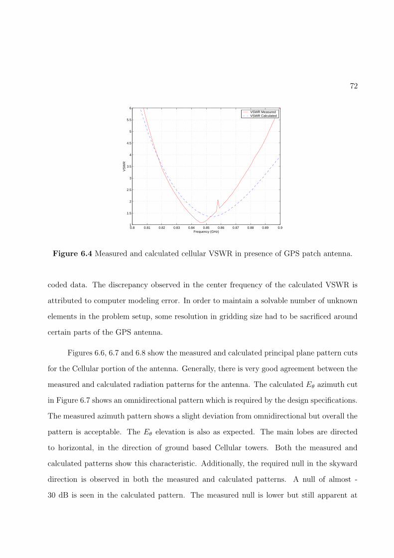
72

0.8 0.81 0.82 0.83 0.84 0.85 0.86 0.87 0.88 0.89 0.91

1.5

2

2.5

3

3.5

4

4.5

5

5.5

6

Frequency (GHz)

VS

WR

VSWR Measured VSWR Calculated

Figure 6.4 Measured and calculated cellular VSWR in presence of GPS patch antenna.

coded data. The discrepancy observed in the center frequency of the calculated VSWR is

attributed to computer modeling error. In order to maintain a solvable number of unknown

elements in the problem setup, some resolution in gridding size had to be sacrificed around

certain parts of the GPS antenna.

Figures 6.6, 6.7 and 6.8 show the measured and calculated principal plane pattern cuts

for the Cellular portion of the antenna. Generally, there is very good agreement between the

measured and calculated radiation patterns for the antenna. The calculated Eθ azimuth cut

in Figure 6.7 shows an omnidirectional pattern which is required by the design specifications.

The measured azimuth pattern shows a slight deviation from omnidirectional but overall the

pattern is acceptable. The Eθ elevation is also as expected. The main lobes are directed

to horizontal, in the direction of ground based Cellular towers. Both the measured and

calculated patterns show this characteristic. Additionally, the required null in the skyward

direction is observed in both the measured and calculated patterns. A null of almost -

30 dB is seen in the calculated pattern. The measured null is lower but still apparent at

73

1.45 1.5 1.55 1.6 1.651

2

3

4

5

6

7

8

9

10

Frequency (GHz)

VS

WR

Measured Calculated

Figure 6.5 GPS measured and calculated VSWR plots.

-16 dB. The calculated gain of the Cellular portion of the antenna is 3 dB. Exact gain

measurements for small antennas are difficult to make, the size of the measurement stand

and cable adapters become appreciable to the size of the antenna. However, the relative

gain measurements made on the far-field range combined with the very close agreement seen

between the calculated patterns and the measured patterns confirm that the actual gain of

the cellular antenna should be close to the design goal of 3 dB.

Figures 6.9 and 6.10 show the measured and calculated principal plane radiation pat-

terns for the GPS portion of the antenna. Close agreement is again seen between the mea-

sured and calculated patterns. The E and H-plane patterns are nominally equal for the

higher elevation angles. There is some distortion in the Eφ cut due to the asymmetrical

location of the patch on the PIFA. The measured patterns show considerably larger nulls in

the backward (-z) direction than the calculated patterns. There is also more ripple observed

in the Eφ pattern in the the backward direction.

74

0 −8 −16 −24 −32 −40 −32 −24 −16 −8 0

30

−150

60

−120

90−90

120

−60

150

−30

180

0

Measured

Calculated

Figure 6.6 Measured and calculated radiation patterns for Cellular antenna of Figure 6.1,

azimuth cut Eφ(θ = 90).

0 −8 −16 −24 −32 −40 −32 −24 −16 −8 0

30

−150

60

−120

90−90

120

−60

150

−30

180

0

Measured

Calculated

Figure 6.7 Measured and calculated radiation patterns for Cellular antenna of Figure 6.1,

azimuth cut Eθ(θ = 90).

75

0 −8 −16 −24 −32 −40 −32 −24 −16 −8 0

30

−150

60

−120

90−90

120

−60

150

−30

180

0

Measured

Calculated

Figure 6.8 Measured and calculated radiation patterns for Cellular antenna of Figure 6.1,

elevation cut Eθ(φ = 90).

As in the Cellular measurments, exact gain values are dificult to measure. However,

the calculated gain values and the close agreement between the calculated radiation patterns

and the measered patterns leads to the conclusion that the actual antenna gain is close to

the 4 dB design specification.

Figure 6.11 show the measured isolation between the two antenna portions. The iso-

lation measurements were preformed on the HP8510 network analyzer. The measurement

spanned the entire frequency range covering both operation frequencies. The measurements

were taken from 0.75 GHz to 1.7 GHz. The maximum coupling seen in the Cellular band is

-27 dB and for the GPS band it is -18 dB. The isolation at the Cellular band is extremely im-

portant because the transmitted Cellular signal is much stronger than the GPS signal. Signal

rejection that can be accomplished through the design of the antenna is advantageous. It is

less unwanted signal that must to be filtered by the receivers.

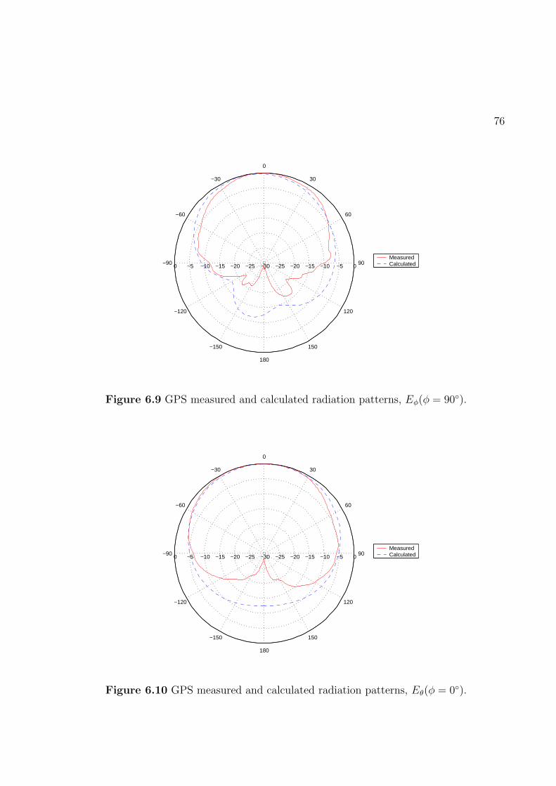
76

0 −5 −10 −15 −20 −25 −30 −25 −20 −15 −10 −5 0

30

−150

60

−120

90−90

120

−60

150

−30

180

0

Measured Calculated

Figure 6.9 GPS measured and calculated radiation patterns, Eφ(φ = 90).

0 −5 −10 −15 −20 −25 −30 −25 −20 −15 −10 −5 0

30

−150

60

−120

90−90

120

−60

150

−30

180

0

Measured Calculated

Figure 6.10 GPS measured and calculated radiation patterns, Eθ(φ = 0).

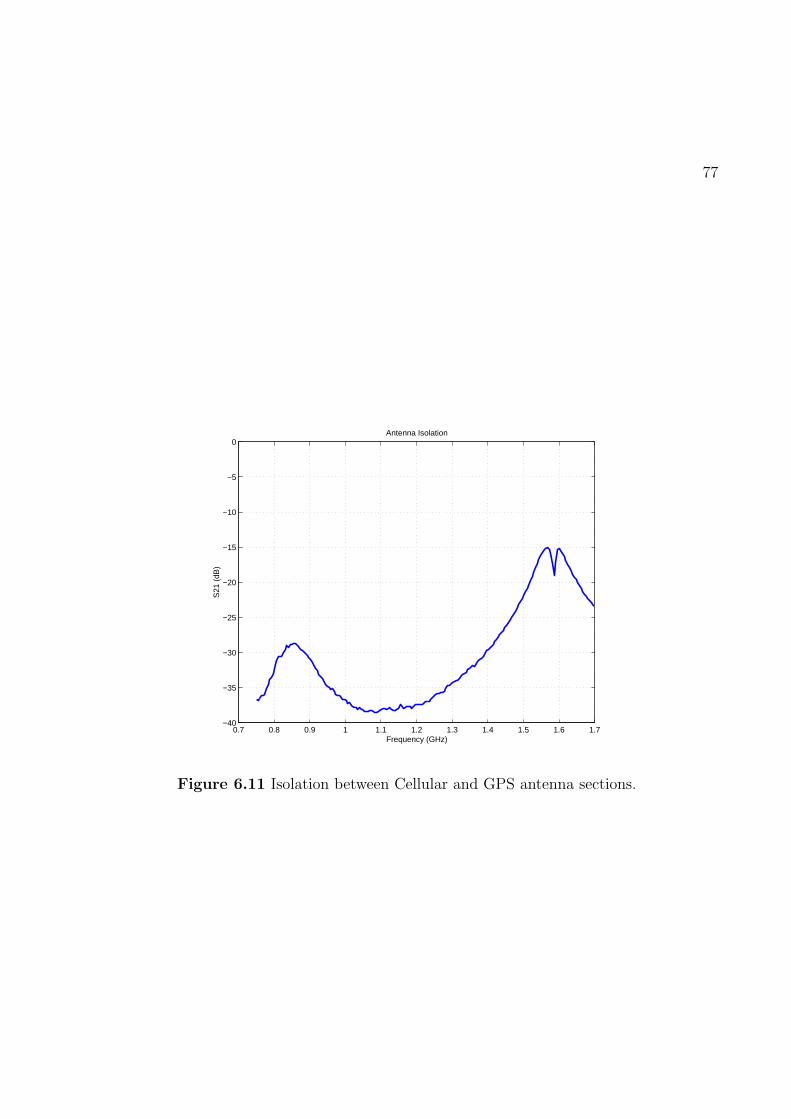
77

0.7 0.8 0.9 1 1.1 1.2 1.3 1.4 1.5 1.6 1.7−40

−35

−30

−25

−20

−15

−10

−5

0

S21

(dB

)

Frequency (GHz)

Antenna Isolation

Figure 6.11 Isolation between Cellular and GPS antenna sections.

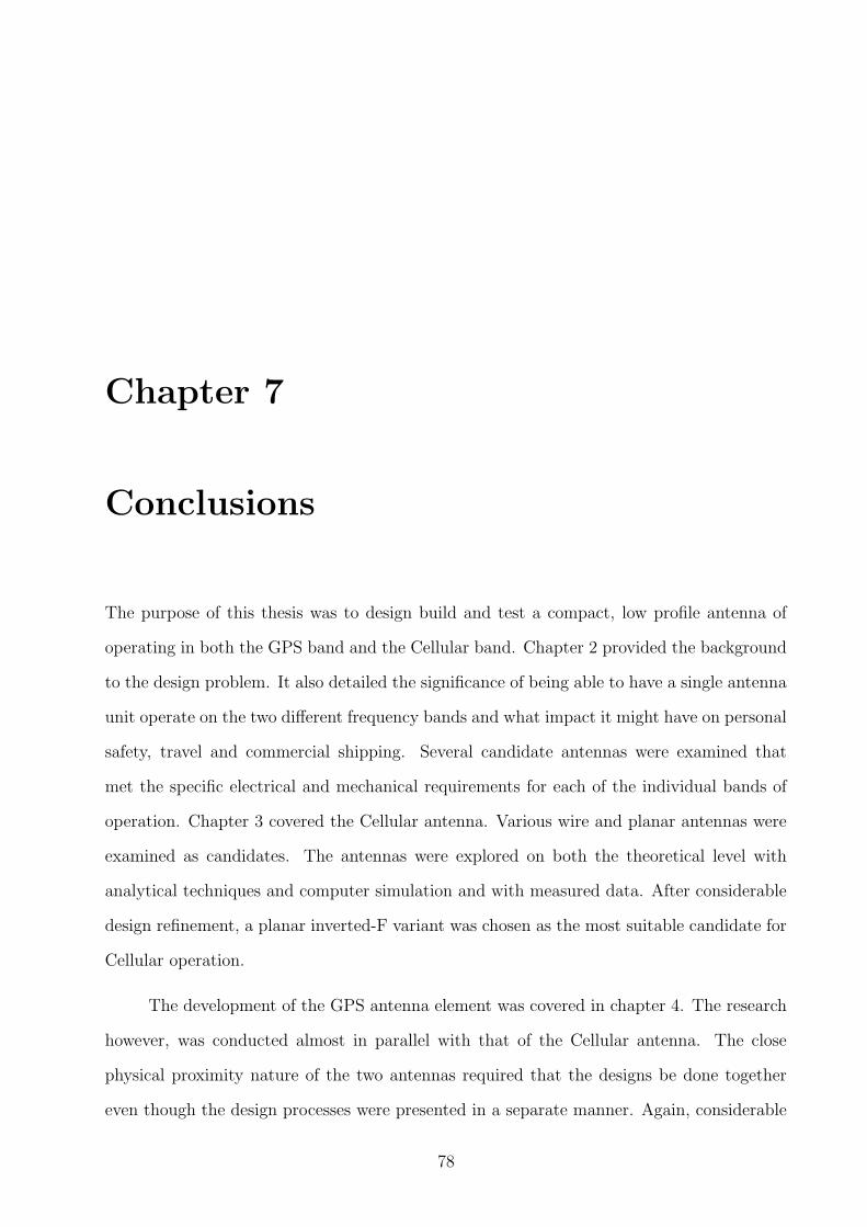
Chapter 7

Conclusions

The purpose of this thesis was to design build and test a compact, low profile antenna of

operating in both the GPS band and the Cellular band. Chapter 2 provided the background

to the design problem. It also detailed the significance of being able to have a single antenna

unit operate on the two different frequency bands and what impact it might have on personal

safety, travel and commercial shipping. Several candidate antennas were examined that

met the specific electrical and mechanical requirements for each of the individual bands of

operation. Chapter 3 covered the Cellular antenna. Various wire and planar antennas were

examined as candidates. The antennas were explored on both the theoretical level with

analytical techniques and computer simulation and with measured data. After considerable

design refinement, a planar inverted-F variant was chosen as the most suitable candidate for

Cellular operation.

The development of the GPS antenna element was covered in chapter 4. The research

however, was conducted almost in parallel with that of the Cellular antenna. The close

physical proximity nature of the two antennas required that the designs be done together

even though the design processes were presented in a separate manner. Again, considerable

78

79

theoretical and experimental analysis was conducted in order to find an appropriate antenna

element for the GPS portion of the combined antenna.

The final design for the integrated antenna presented in Chapter 6 met nearly all of

the design goals. The Measured operating frequency and bandwidth for both the Cellular

and GPS portions were a little lower than the design specifications but very acceptable as

starting for a final evaluation and design modification. The measured radiation patterns

in both cases produced acceptable results. The combination of computer simulation and

relative gain measurements leads to the conclusion that the actual gain of the GPS antenna

was within the acceptable limits even though exact gain measurements available at the test

facility. The measured isolation between the two antenna portions also gave desirable results.

Possible future work for this project could include incorporating a single feed for both

the GPS and the Cellular elements. Additionally, the integration of a low noise amplifier for

the GPS unit is also an area to investigate as well as improving the element isolation.

Vita

Nathan P. Cummings was born in January 1975 in Parkersburg, West Virginia. He spent hisentire precollegiate life on the same street in the town of Vienna, a suburb of Parkersburg. Hegraduated from high school in 1993 and began his studies in Electrical Engineering at VirginiaPolytechnic Institute & State University in the fall of that year. His undergraduate tenureincluded a co-op position with G.E. Fanuc Automation, North America in Charlottesville,VA. He received his B.S.E.E. from Virginia Tech in May of 1998. Upon completion of hisundergraduate degree he joined the Virginia Tech Antenna Group. Nathan is continuing topursue scholarly research endeavors for VTAG.

80