low-order modelling of thermoacoutic limit cycles - iwr

March 5, 2004 0:20

Proceedings of ASME TURBO EXPO 2004Power for Land, Sea, and Air

June 14–17, 2004, Vienna, Austria

GT2004-54245

LOW-ORDER MODELLING OF THERMOACOUSTIC LIMIT CYCLES

Simon R. Stow and Ann P. DowlingDepartment of Engineering, University of Cambridge

Cambridge, CB2 1PZ, United KingdomTel: +44 1223 332600, Fax: +44 1223 332662, E-mail: [email protected]

ABSTRACTLean premixed prevaporised (LPP) combustion can reduce

NOx emissions from gas turbines, but often leads to combustioninstability. Acoustic waves produce fluctuations in heat release,for instance by perturbing the fuel-air ratio. These heat fluctua-tions will in turn generate more acoustic waves and in some sit-uations self-sustained oscillations can form. The resulting limitcycles can have large amplitude causing structural damage.

Thermoacoustic oscillations will have a low amplitude ini-tially. Thus linear models can give stability predictions. An un-stable linear mode will grow in amplitude until nonlinear effectsbecome important and a limit cycle is achieved. While the fre-quency of the linear mode can provide a good approximation tothat of the resulting limit cycle, linear theories give no predictionof its amplitude.

A low-order model for thermoacoustic limit cycles in LPPcombustors is described. The approach is based on the fact thatthe main nonlinearity is in the combustion response to flow per-turbations. In LPP combustion, fluctuations in the inlet fuel-airratio have been shown to be the dominant cause of unsteady com-bustion: these occur because velocity perturbations in the premixducts cause a time-varying fuel-air ratio, which then convectsdownstream. If the velocity perturbation becomes comparable tothe mean flow, there will be an amplitude-dependent effect on theequivalence ratio fluctuations entering the combustor and henceon the rate of heat release. A simple nonlinear flame model forthis dependence is developed and is assumed to be the major non-linear effect on the limit cycle. Since the Mach number is low,the velocity perturbation can be comparable to the mean flow,with even reverse flow occurring, while the disturbances are stillacoustically linear in that the pressure perturbation is still much

smaller than the mean. Hence elsewhere the perturbations aretreated as linear. In this nonlinear flame model, the flame transferfunction describing the combustion response to changes in inletflow is a function of both frequency and amplitude. The nonlin-ear flame transfer function is incorporated into a linear thermoa-coustic network model for plane waves. Frequency, amplitudeand modeshape predictions are compared with results from an at-mospheric test rig. The approach is extended to circumferentialwaves in a thin annular geometry, where the nonlinearity leads tomodal coupling.

NOMENCLATUREAu amplitude of velocity perturbation divide by meanp pressureQ heat releaset timeTQ,u nonlinear flame transfer function (relatingQ to u)u axial velocityw circumferential velocityx axial coordinateθ circumferential coordinateρ densityτ fuel convection time for mean flowφ equivalence ratioω complex frequency

Superscripts() unperturbed value()′ perturbation() complex perturbation, assuming factor of eiωt

1 Copyright 2004 by ASME

http://www.eng.cam.ac.uk/~srs31

http://www.eng.cam.ac.uk/~apd1

http://www.eng.cam.ac.uk

http://www.cam.ac.uk

mailto:[email protected]

1 INTRODUCTIONLPP combustion is a method of reducing NOx emissions

from gas turbines by mixing the fuel and air more evenly be-fore combustion. However LPP combustion is highly susceptibleto thermoacoustic oscillations. The interaction between soundwaves and combustion can lead to large pressure fluctuations, re-sulting in structural damage. Linear models can give predictionsfor the frequency and linear stability of oscillations, and thus in-dicate possible modes. However they do not give predictions ofoscillation amplitude. Ideally one would wish to design a com-bustion system that is linearly stable, however this may not bepossible. Thus models that can predict limit-cycle amplitude arerequired to help design combustors that oscillate within accept-able bounds. Furthermore, such models can be used to investi-gate the potential amplitude reduction from damping devices.

We present a low-order theory to predict limit cycles in LPPcombustors. The theory uses a describing-function approachcombines a linear thermoacoustic model with a nonlinear com-bustion model. The thermoacoustic model, described in Sec-tion 2, is formulated in terms of a network of modules describ-ing the features of the geometry. The model can be applied ei-ther to long combustors (typical of industrial gas turbines) wherethe perturbations can be treated as one-dimensional, or to shortthin-annular combustors (typical of aeroengines) where the per-turbations can be treated as circumferential waves. There havebeen several studies on linear combustion-instability models inthe literature. For example, Paschereit et al. [1] described an ap-proach in which the premixer and combustion zone are modelledby a single transfer matrix. The coefficients of the matrix werefound experimentally by using loud-speaker forcing in a test rig.Kruger et al. [2, 3] have used networks of one-dimensional mod-ules linked together in both axial and circumferential directionsto model annular combustors. Oscillations in annular combus-tors have also been computed by Hsiao et al. [4, 5] using a hy-brid CFD/acoustics-based model on a three-dimensional grid ofcells. A review of linear modelling of combustion instability isgive in [6]. Nonlinear modelling of thermoacoustic oscillationswas first motivated by instability in rocket engines (see for exam-ple [7, 8]). For LPP combustion, nonlinear time-domain modelshave been developed to calculate limit cycles [9, 10, 11].

There is much evidence that equivalence ratio fluctuationsare the dominant cause of heat-release oscillations in LPP com-bustors (see for example [12, 13]). The combustion model (Sec-tion 3) accounts for the amplitude-dependent effect on the equiv-alence ratio when the velocity perturbation becomes comparableto the mean flow in the premix ducts. It is assumed that thisis the main source of nonlinearity determining the amplitude ofthe limit cycle. The calculation of the heat release is done inthe time domain, then converted to the frequency domain andincorporated into the thermoacoustic model using a describing-function approach. This is very similar to the technique usedby Dowling [14] to predict the limit cycle for one-dimensional

waves with a fully-premixed ducted flame stabilised on a bluffbody, and works well when there is a periodic limit cycle andthe flame response to forcing decreases with amplitude, whichis often the case in a combustion instability. The extension tocircumferential waves introduces modal coupling.

In Section 6, we compare predictions from the theory withexperimental results for an atmospheric test rig. Finally, our con-clusions are presented in Section 7.

2 LINEAR THERMOACOUSTIC NETWORK MODELBefore investigating nonlinear effects, we give a brief de-

scription of the linear combustion-instability model. We usecylindrical polar coordinatesx, r andθ and write the pressure,density, temperature and velocity asp, ρ, T and (u,v,w), re-spectively. We will assume a perfect gas,p = RgasρT. Theflow is taken to be composed of a steady axial mean flow (de-noted by bars) and a small perturbation (denoted by dashes).We make one of two assumptions about the combustor geom-etry: either we assume it is axially long (typical of industrialgas turbines) or that it has a narrow annular cross-section (typ-ical of aeroengines). The mean flow for either cases can be as-sumed to be one-dimensional. For the former case, the pertur-bations will also be one-dimensional (at least at frequencies ofpractical interest). In the latter case, circumferential variation ofthe perturbation could be important but radial variation can beneglected. We consider perturbations with complex frequencyω, i.e. we havep = p(x)+ p′(x,θ , t) with p′ = Re[p(x,θ)eiωt ],(and similarly for the other flow variables). We may considerthe perturbations as a sum of circumferential modes by writingp(x,θ) = ∑N

n=−N pneinθ and so on (whereN is sufficiently largethat the higher-order modes can be neglected). If the geometryis axisymmetric throughout then the circumferential modes canbe considered independently. However if the symmetry is bro-ken (for instance by a Helmholtz resonator being present [15])the modes can become coupled and must be calculated together.Note that for the case of a one-dimensional geometry, only theplane waves are present and we simply haveN = 0.

The geometry is composed of a network of modules describ-ing its features, such as straight ducts, area changes and combus-tion zones. For the straight ducts modules, wave propagation isused to relate the perturbations at one end of the duct to thoseat the other. The rest of the modules are assumed to be acous-tically compact. Here quasi-steady conversation laws for mass,momentum and energy are used to find the perturbations. Ata combustion zone, the unsteady heat release is related to theflow disturbances by a (linear) flame transfer function. Acousticboundary conditions are assumed to be known at the inlet andoutlet of the geometry. The procedure to find the resonant modesis to guess an initial value forω and calculate the perturbations,starting at the inlet and stepping through the modules to the out-let. In general this solution will not match the outlet boundary


condition. ω is then iterated to satisfy this constraint. (For cou-pled circumferential modes, the relative phase and magnitude ofthe modes at the inlet must also be calculated.) The frequency ofthe mode is then Re(ω)/(2π), and we define the growth rate as− Im(ω). If the growth rate is negative the mode is linearly sta-ble and would not be expected to be seen in practice, whereas ifthe growth rate is positive the mode is unstable at would grow inamplitude until nonlinear effects become important and a limitcycle is achieved. More details on this linear model are givenin [16], with the procedure for coupled circumferential modesdescribed in [15].

The above references only consider geometries with a singleflow-pathway from the inlet to the outlet, however it is possibleto extend the model to have multiple pathways. These additional‘secondary paths’ may originate by splitting of the flow or fromsecondary inlets to the geometry. The paths can later terminateas dead ends, or by joining into other paths. Flow from one pathto another through holes can also be incorporated. This meansthat cooling flows and staged combustion can be modelled. Atthe start of each secondary path there is an unknown parameterfor the perturbation (such as the ratio of the mass-flux pertur-bations at a flow split), and at the end of each path there is aboundary condition (such as û = 0 at a dead end). However,due to the linearity of the model, calculation of these simplyinvolves the solution of a(P+ 1)-dimensional complex matrixequation (or(P+1)(2N+1)-dimensional for coupled circumfer-ential modes). This extension to the linear model will be describein a future publication. A general review of linear methods forcombustion instability in LPP gas turbines in given [6].

3 NONLINEAR FLAME MODELWe now consider a simple nonlinear flame model relating

heat release perturbations to velocity perturbations in the premixducts. We consider harmonic oscillations with real frequency. Atthe fuel injection point in the premix ducts, we have

u′(t) = Re(ueiωt) = |u|cos(ωt +argu), (1)

where the complex amplitude û = |u|eiargu. We writeAu = |u|/uand initially take û to be real and positive, hence

u(t) = u(1+Aucosωt). (2)

If Au 6 1 there is no reverse flow, however ifAu > 1 there is flowreversal during part of the cycle. We consider these two casesseparately.

3.1 No reverse flowLPP flames are typically short, and in acoustically-forced

experiments Armitage et al. [17] found little phase variation

along the flame (the corresponding convection time being lessthan 0.5 ms). Hence we assume that combustion takes place in aplane. Moreover, chemiluminescence shows significant changein amplitude over a cycle, but little change in location. Thechange in convective time delay associated with any slight shiftin the location is negligible compared with the period of oscil-lations and so we consider the plane of combustion to be at afixed distance,L, downstream of fuel injection. Since the Machnumber is low and the premixers are short, we will ignore com-pressibility effects here. We also assume that the (unsteady) ve-locity does not vary axially along this section, i.e. the region isacoustically compact. Hence, assuming a choked fuel supply, theequivalence ratio at combustion is

φ(t) = φ f (t f ) = φu

u(t f ), (3)

whereφ f is the equivalence ratio at the fuel injection point andt f (t) is the time at which the fuel was injected. (Note thatφ

is defined as the equivalence ratio that would be present for anundisturbed flow, i.e.Au = 0. For nonlinear oscillations, this isnot necessarily equal to the time average ofφ(t).) t − t f is theunsteady fuel convection time and

L =∫ t

t f

u(t)dt = uτ, (4)

whereτ is the fuel convection time for mean flow conditions.Substituting foru from Eq. (2) gives

F [t f ] = t− t f +Ausinωt−sinωt f

ω− τ = 0. (5)

Solving this equation iteratively givest f (t) and henceφ(t).In the above we have assumed a single mean convection

time. If the mean flow profile was non-uniform, there would in-stead be a distribution in time delays [18]. A similar effect wouldbe seen if the flame had significant axial distrubution [19], or ifmultiple fuel injection points were present. Such effects couldeasily be incorporated into the model.

3.2 Reverse flowIf there is reverse flow, a fluid particle may pass the point of

fuel injection more than once, see Fig. 1. Ignoring the mass offuel in the mixture compared to the mass of the air (as was doneabove implicitly) we have

φ(t) = ∑t f∈S

φ f (t f ) = ∑t f∈S

φu

u(t f ), (6)


fuel flame

Figure 1. Schematic diagram of a particle path in reverse flow. The fluid

particle passes the fuel injection point and flame zone multiple times.

Fuel is added at several times, but only burns once.

whereS (t) = {t f : F [t f ] = 0} is the set of all the times at whichthe current fluid particle has passed the fuel injectors,F [t f ] beingas defined in Eq. (5). By considering the maxima and minima ofthe functionF [t f ], for a givent we can deduce the number ofroots and bounds for their location. Hence all the solutions canbe found numerically and we may then calculateφ(t).

However, there is one further consideration. Just as the fluidparticle can pass the fuel injectors more than once, it may alsopass the flame zone more than once (see Fig. 1). In this simplemodel, it is appropriate to setφ(t) = 0 if the fluid particle haspreviously crossed the flame meaning the fuel has already beenburnt. For a fluid particle currently at the flame (i.e. at timet), byintegrating Eq. (2) its position relative to the flame at an earliertime, te, is

x(te) = u(

te− t +Ausinωte−sinωt

ω

). (7)

By considering the maxima of this function, for a givent we cancheck if the fluid particle has previously crossed the combustionzone, i.e. ifx(te) > 0 for somete < t. If it has we setφ(t) = 0,whereas if not we calculateφ(t) as above.

3.3 Combustion modelHaving calculatedφ(t) as described in Section 3.1 or 3.2,

we now need a model to relate this to the heat release,Q(t). Anestimate of the heat release per unit mass is

∆H(φ) =

{φ∆Hs, 0 6 φ < 1,

∆Hs, φ > 1,(8)

where∆Hs is the value at stoichiometric conditions. To illustratethe approach we will use the following simple model for the heatrelease

Q(φ) ∝ ∆H(φ), (9)

however a more sophisticated model could easily used instead.For instance, the effect of lean blow-out could be incorporatedby definingQ to be zero forφ below a critical value.

3.4 Conversion to the frequency domainThe nonlinear flame model presented above is in the time

domain, whereas the (linear) thermoacoustic model in Section2 is in the frequency domain. To estimate the amplitude andfrequency of the limit cycle, we use describing function analysisto convert the flame model to the frequency domain (as used byDowling [14] for a fully-premixed ducted flame). Since the inputto the flame model (u(t) at the premixers) was assumed to beharmonic, its output (Q(t)) will have the same period, though ingeneral it will be non-harmonic. HenceQ(t) can be described bya Fourier series,

Q(t) = a0 +∞

∑m=1

amcos(mωt +ψm)

= Q0 +Re( ∞

∑m=1

Qmeimωt).

(10)

(Here Q0 is the time average ofQ(t).) Experimental pres-sure spectra for self-excited oscillations show that harmonics arepresent, but are not strong. Furthermore, we expect that the flamewill not respond to high-frequency disturbances. This suggeststhat onlyQ1, the component at the driving frequencyω, is im-portant in the feedback loop between the heat release and theacoustics of the geometry. Thus to find a solution in the fre-quency domain, we ignore the higher-frequency terms and takeQ = Q1. We can then define a nonlinear flame transfer function,

TQ,u(ω,Au) =Q/Qu/u

=ω

πAu

∫ 2π/ω

0Q(t)e−iωtdt. (11)

It was originally assumed that û was real. For complex û there isa phase adjustment toQ. This has been included in the formula-tion of Eq. (11) and so it is still valid for complex û.

We can also define a linearised flame transfer function,

TLQ,u(ω) = lim

Au→0TQ,u(ω,Au). (12)

Assuming a single mean convection time, as in Section 3.1,

TLQ,u(ω) =

φ

Q

dQdφ

e−iωτ =−e−iωτ , (13)

for the combustion model in Eq. (9). It should be noted that asimple time-delay flame model of this form has been used exten-sively in the literature [20, 21] and shown to compare well withexperimental data from some simple rigs.


0 0.5 1 1.5 20

0.5

1

Au

|TQ

,u /

T Q,u

L|

0 0.5 1 1.5 2−1

−0.5

0

0.5

1

Au

phas

e (T

Q,u

/ T Q

,uL

) / π

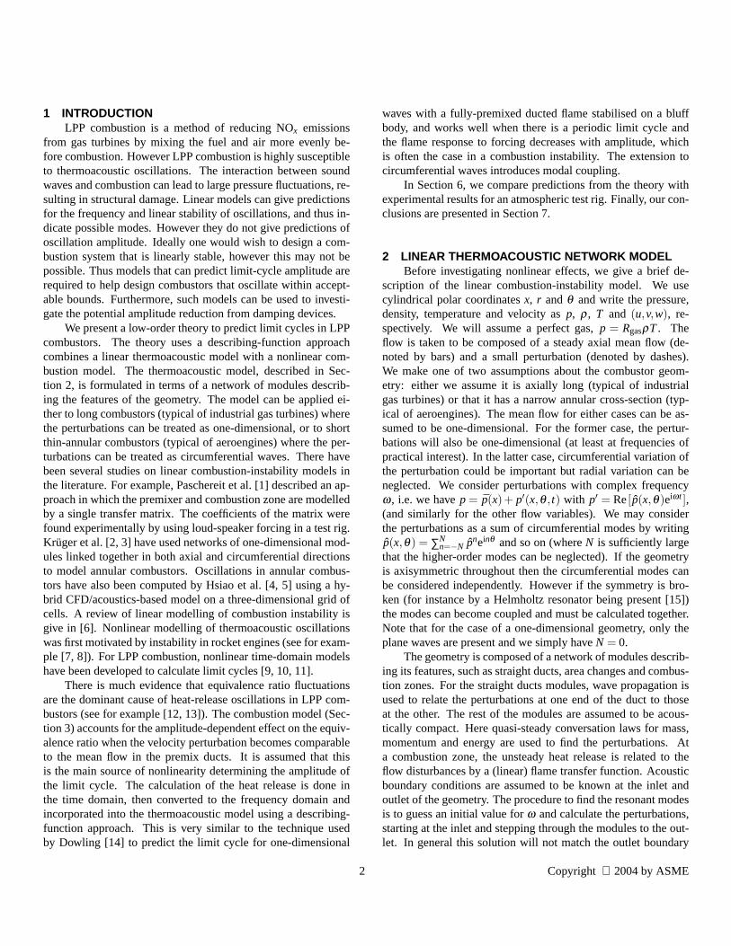
Figure 2. Variation of TQ,u/TLQ,u with Au for φ = 0.7. The solid,

dashed, dash–dotted and dotted lines denote ωτ/π (mod 1) = 0,

0.25, 0.5 and 0.75, respectively.

Although not used in the calculation ofQ, we can definea nonlinear transfer function relating equivalence ratio perturba-tions to velocity perturbations in the frequency domain as fol-lows,

Tφ ,u(ω,Au) =φ/φ

u/u=

ω

πAu

∫ 2π/ω

0φ(t)e−iωtdt. (14)

with a linearised version,

TLφ ,u(ω) = lim

Au→0Tφ ,u(ω,Au) =−e−iωτ . (15)

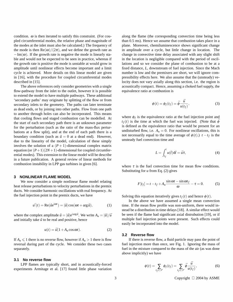
Note that it can be deduced from Eq. (5) and Eq. (11) that theonly parameters controllingTQ,u andTφ ,u areωτ (mod 2π), Au

andφ . Figures 2 and 3 show the variation ofTQ,u/TLQ,u with Au

andωτ for φ = 0.7. The value must be unity forAu = 0 from thedefinition ofTL

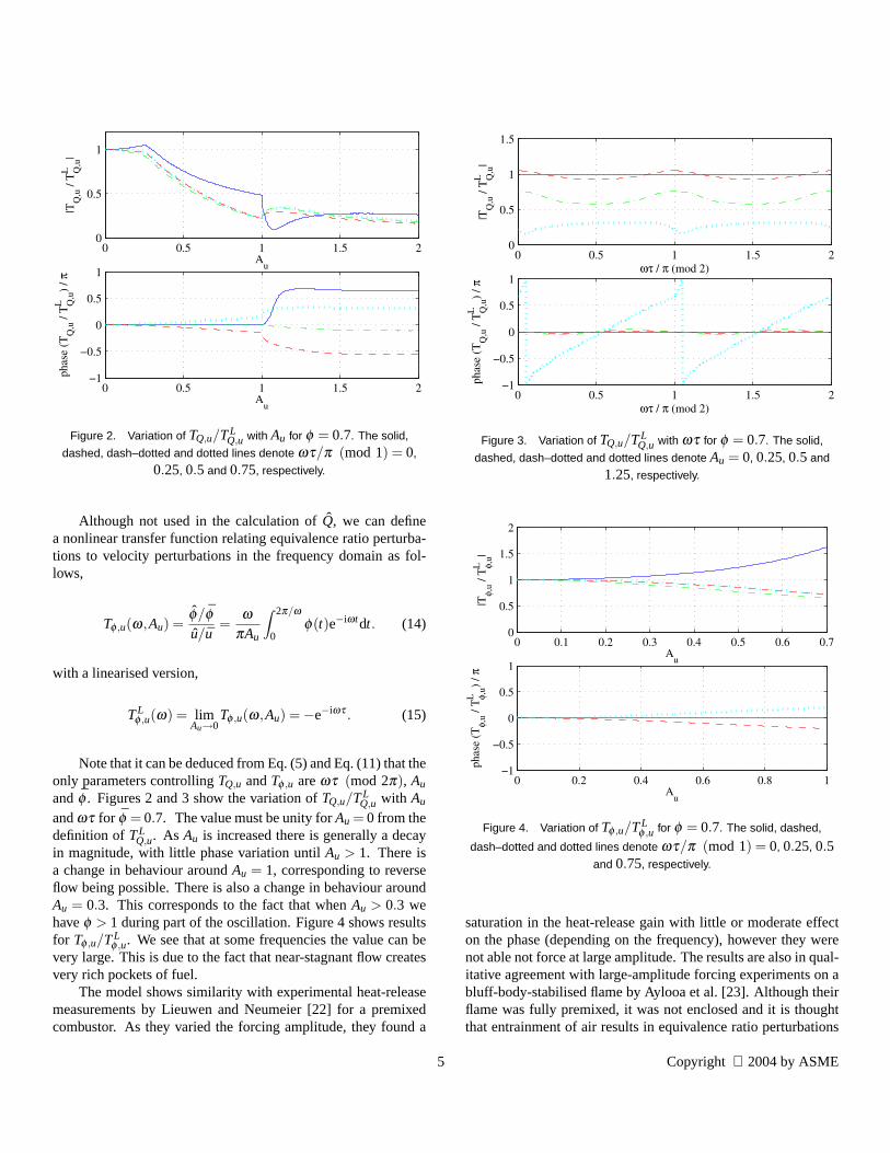
Q,u. As Au is increased there is generally a decayin magnitude, with little phase variation untilAu > 1. There isa change in behaviour aroundAu = 1, corresponding to reverseflow being possible. There is also a change in behaviour aroundAu = 0.3. This corresponds to the fact that whenAu > 0.3 wehaveφ > 1 during part of the oscillation. Figure 4 shows resultsfor Tφ ,u/TL

φ ,u. We see that at some frequencies the value can bevery large. This is due to the fact that near-stagnant flow createsvery rich pockets of fuel.

The model shows similarity with experimental heat-releasemeasurements by Lieuwen and Neumeier [22] for a premixedcombustor. As they varied the forcing amplitude, they found a

0 0.5 1 1.5 20

0.5

1

1.5

ωτ / π (mod 2)

|TQ

,u /

T Q,u

L|

0 0.5 1 1.5 2−1

−0.5

0

0.5

1

ωτ / π (mod 2)

phas

e (T

Q,u

/ T Q

,uL

) / π

Figure 3. Variation of TQ,u/TLQ,u with ωτ for φ = 0.7. The solid,

dashed, dash–dotted and dotted lines denote Au = 0, 0.25, 0.5 and

1.25, respectively.

0 0.1 0.2 0.3 0.4 0.5 0.6 0.70

0.5

1

1.5

2

Au

|Tφ,

u / T φ,

uL

|

0 0.2 0.4 0.6 0.8 1−1

−0.5

0

0.5

1

Au

phas

e (T

φ,u /

T φ,u

L) /

π

Figure 4. Variation of Tφ ,u/TLφ ,u for φ = 0.7. The solid, dashed,

dash–dotted and dotted lines denote ωτ/π (mod 1) = 0, 0.25, 0.5and 0.75, respectively.

saturation in the heat-release gain with little or moderate effecton the phase (depending on the frequency), however they werenot able not force at large amplitude. The results are also in qual-itative agreement with large-amplitude forcing experiments on abluff-body-stabilised flame by Aylooa et al. [23]. Although theirflame was fully premixed, it was not enclosed and it is thoughtthat entrainment of air results in equivalence ratio perturbations


similar to the process in the fuel injectors of an LPP system. Onedifference however is that the flow can never develop rich pock-ets, and hence they did not see a change in the flame transferfunction behaviour forAu > 1.

4 LIMIT-CYCLE CALCULATIONSWe now consider how nonlinear flame transfer functions can

be incorporated into the linear network model to give predictionsof limit-cycle frequency and dimensional modeshapes. Providedthere is only one (nonlinear) combustion zone present, the proce-dure is relatively straightforward and is described first. We thenexplain an approach for multiple combustion zones.

4.1 Single combustion zoneNonlinearity occurs when the flow is linearly unstable. So

that with TLQ,u(ω) the network analysis gives a complex fre-

quencyω, with positive growth rate (− Im(ω)). As the ampli-tude of the resulting oscillation increases,TQ,u changes and alimit cycle in which the growth rate is zero occurs at the am-plitudeAu that makesω real. This limit cycle is stable in time;if the amplitude is greater thanAu, − Im(ω) < 0 and the oscil-lation decreases in amplitude, while for amplitudes less thanAu

it increases. So if there is only one nonlinear combustion zonein the geometry, the unknown variables that determine the limitcycle are now (real)ω andAu, instead of complexω for a linearcalculation. We may guess initial values forω andAu and cal-culate a non-dimensional perturbation solution in the usual way,using the heat release given by the nonlinear flame transfer func-tions. These two unknown can then be iterated to satisfy both thereal and imaginary part of the outlet error being zero. This givesthe limit-cycle frequency and a non-dimensional modeshape. Tofind the dimensional modeshape, the perturbations are scaled tobe consistent with the calculated value ofAu. That is, the dimen-sional solution is give by multiplying the non-dimensional by thefactorAuu/|u|, evaluated at the fuel injectors.

An alternative method of calculation is to fixAu and calcu-late complexω to satisfy the outlet boundary condition in theusual way. The nonlinear flame model developed in Section 3 isonly valid for realω, and so we setω = Re(ω) in Eq. (11). Be-cause of this, solutions thus found are not truly valid, in partic-ular the value of the growth rate does not have a physical mean-ing. (The nonlinear flame model could be extended to complexω, but there appears to be little benefit in this.) However, it isclear that if the growth rate is found to be zero, the solution is avalid limit cycle. If we iterateAu to make the growth rate zerowe should find the same limit-cycle solutions as before. Thisdouble-iteration method will be less numerically efficient, but al-lows an appealing calculation procedure: We may first calculatethe linear modes of the system using the linear flame transferfunction Eq. (12). This is equivalent to settingAu = 0. For any

unstable modes, we may then increase the value ofAu, calculat-ing the resulting complexω, until the growth rate value is zero.This will give the resulting limit cycle. (This method should alsoensure that the limit cycle is stable, i.e. there is growth for loweramplitudes and decay for higher amplitudes.)

4.2 Multiple combustion zonesIf we have more than one combustion zone modelled non-

linearly, the above calculation procedures cannot be used be-cause the flame-model amplitudes are interdependent. Instead,we guess initial values for the (real) limit-cycle frequency andthe dimensional perturbations at the main inlet. The linearityused to calculate any flow splits and/or secondary inlets is alsono longer valid. Hence the (dimensional) parameters there mustalso be included in the iteration. Having guessed initial values ofthese parameters, we may calculate the perturbations as usual tofind the error at the (main) outlet and the end of each secondarypath. This leads to a 2(P+ 1)-dimensional system of equationswhich can be solved using a discrete Newton-Raphson methodto give the frequency and dimensional modeshape.

5 CIRCUMFERENTIAL WAVESSo far we have only considered plane waves. We now con-

sider circumferential waves in thin annular combustors, typicalof aeroengines. In such a geometry, radial variation is not sig-nificant and we can write the flow variable in the formp′ =Re[p(x,θ)eiωt ], with p(x,θ) = ∑N

n=−N pneinθ , etc. More detailson this approach are given in [15] for linear modelling. Here weshall concentrate on modelling the combustion zone and the cal-culation of limit cycles. We begin by discussing how a ring ofpremix ducts affects the circumferential waves.

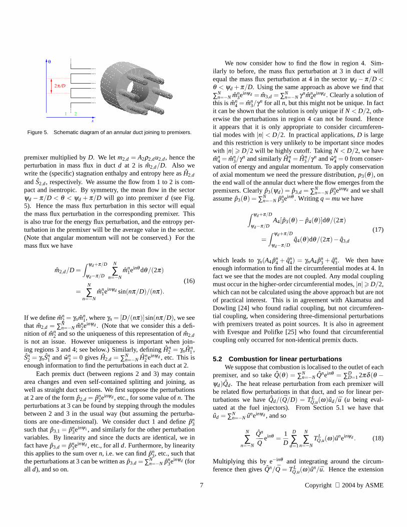
5.1 Premix ductsWe assume that fuel is injected in a ring of premix ducts

joining the annular plenum and combustion chambers. We con-sider D identical premix ducts centred atθ = ψ1,ψ2, . . . ,ψD,whereψd = 2πd/D (see Fig. 5). These are assumed to have asmall cross-sectional area and so the perturbations in them aretaken to be one-dimensional. In the following we will take the(specific) stagnation enthalpy to beH, the entropy to beS andthe mass flow rate to bem = Aρu, A being the cross-sectionarea. We define regions 1 and 4 to be in the annular ductsjust before and just after the premix ducts, respectively. Herethe perturbations can be written as ˆp1(x,θ) = ∑N

n=−N pn1einθ and

p4(x,θ) = ∑Nn=−N pn

4einθ , etc. We define regions 2 and 3 to bein the premix ducts just after they start and just before they fin-ish, respectively. We denote the flow in ductd by p2,d andp3,d,etc. Hence in particular since the flow in the ducts is assumedone-dimensional, ˆw2,d = w3,d = 0. We defineA2 to be the to-tal area of the ducts at region 2, i.e. the inlet area of a single


x

θ

1 2

π2 /D

Figure 5. Schematic diagram of an annular duct joining to premixers.

premixer multiplied byD. We letm2,d = A2ρ2,du2,d, hence theperturbation in mass flux in ductd at 2 is m2,d/D. Also wewrite the (specific) stagnation enthalpy and entropy here asH2,d

andS2,d, respectively. We assume the flow from 1 to 2 is com-pact and isentropic. By symmetry, the mean flow in the sectorψd − π/D < θ < ψd + π/D will go into premixerd (see Fig.5). Hence the mass flux perturbation in this sector will equalthe mass flux perturbation in the corresponding premixer. Thisis also true for the energy flux perturbation, and the entropy per-turbation in the premixer will be the average value in the sector.(Note that angular momentum will not be conserved.) For themass flux we have

m2,d/D =∫

ψd+π/D

ψd−π/D

N

∑n=−N

mn1einθ dθ/(2π)

=N

∑n=−N

mn1einψd sin(nπ/D)/(nπ).

(16)

If we definemn2 = γnmn

1, whereγn = [D/(nπ)]sin(nπ/D), we seethat m2,d = ∑N

n=−N mn2einψd . (Note that we consider this a defi-

nition of mn2 and so the uniqueness of this representation of ˆm2,d

is not an issue. However uniqueness is important when join-ing regions 3 and 4; see below.) Similarly, definingHn

2 = γnHn1 ,

Sn2 = γnSn

1 andwn2 = 0 givesH2,d = ∑N

n=−N Hn2einψd , etc. This is

enough information to find the perturbations in each duct at 2.Each premix duct (between regions 2 and 3) may contain

area changes and even self-contained splitting and joining, aswell as straight duct sections. We first suppose the perturbationsat 2 are of the form ˆp2,d = pn

2einψd , etc., for some value ofn. Theperturbations at 3 can be found by stepping through the modulesbetween 2 and 3 in the usual way (but assuming the perturba-tions are one-dimensional). We consider duct 1 and define ˆpn

3such that ˆp3,1 = pn

3einψ1, and similarly for the other perturbationvariables. By linearity and since the ducts are identical, we infact have ˆp3,d = pn

3einψd , etc., for alld. Furthermore, by linearitythis applies to the sum overn, i.e. we can find ˆpn

3, etc., such thatthe perturbations at 3 can be written as ˆp3,d = ∑N

n=−N pn3einψd (for

all d), and so on.

We now consider how to find the flow in region 4. Sim-ilarly to before, the mass flux perturbation at 3 in ductd willequal the mass flux perturbation at 4 in the sectorψd −π/D <θ < ψd + π/D. Using the same approach as above we find that∑N

n=−N mn3einψd = m3,d = ∑N

n=−N γnmn4einψd . Clearly a solution of

this ismn4 = mn

3/γn for all n, but this might not be unique. In factit can be shown that the solution is only unique ifN < D/2, oth-erwise the perturbations in region 4 can not be found. Henceit appears that it is only appropriate to consider circumferen-tial modes with|n| < D/2. In practical applications,D is largeand this restriction is very unlikely to be important since modeswith |n| > D/2 will be highly cutoff. TakingN < D/2, we havemn

4 = mn3/γn and similarlyHn

4 = Hn3/γn andwn

4 = 0 from conser-vation of energy and angular momentum. To apply conservationof axial momentum we need the pressure distribution,p3(θ), onthe end wall of the annular duct where the flow emerges from thepremixers. Clearly ˆp3(ψd) = p3,d = ∑N

n=−N pn3einψd and we shall

assume ˆp3(θ) = ∑Nn=−N pn

3einθ . Writing q = muwe have

∫ψd+π/D

ψd−π/DA4[p3(θ)− p4(θ)]dθ/(2π)

=∫

ψd+π/D

ψd−π/Dq4(θ)dθ/(2π)− q3,d

(17)

which leads toγn(A4pn4 + qn

4) = γnA4 pn3 + qn

3. We then haveenough information to find all the circumferential modes at 4. Infact we see that the modes are not coupled. Any modal couplingmust occur in the higher-order circumferential modes,|n|> D/2,which can not be calculated using the above approach but are notof practical interest. This is in agreement with Akamatsu andDowling [24] who found radial coupling, but not circumferen-tial coupling, when considering three-dimensional perturbationswith premixers treated as point sources. It is also in agreementwith Evesque and Polifke [25] who found that circumferentialcoupling only occurred for non-identical premix ducts.

5.2 Combustion for linear perturbationsWe suppose that combustion is localised to the outlet of each

premixer, and so takeQ(θ) = ∑Nn=−N Qneinθ = ∑D

D=12πδ (θ −ψd)Qd. The heat release perturbation from each premixer willbe related flow perturbations in that duct, and so for linear per-turbations we haveQd/(Q/D) = TL

Q,u(ω)ud/u (u being eval-uated at the fuel injectors). From Section 5.1 we have thatud = ∑N

n=−N uneinψd , and so

N

∑n=−N

Qn

Qeinθ =

1D

D

∑d=1

N

∑n=−N

TLQ,u(ω)uneinψd . (18)

Multiplying this by e−inθ and integrating around the circum-ference then givesQn/Q = TL

Q,u(ω)un/u. Hence the extension


of linear combustion modelling from planes to circumferentialwaves is straightforward. In particular, no modal coupling is in-troduced.

5.3 Nonlinear combustion and limit-cycle calculationFor nonlinear combustion with circumferential waves, the

velocity amplitude in each premix ductAu,d must be considered.Using the same approach as in Section 5.2 we find that

Qn

Q=

1D

D

∑d=1

TLQ,u(ω,Au,d)un/u, (19)

with Au,d = ud/u = ∑Nn=−N un

3einψd , and hence the circumferen-tial modes are now coupled. This expression for the heat releaseperturbations can then be used to calculate limit cycles by thesame approach as in Section 4.2, except that we must now iter-ate for each circumferential component of the path parameters,implying a 2(P+1)(2N+1)-dimensional system.

6 RESULTSWe now compare the above model with experimental results

for an atmospheric test rig. This consists of axially long plenumand combustion chambers joined by single LPP swirler unit. Theinlet to the plenum is choked and the combustor exits to the at-mosphere (hence acoustically it is an open end). The dimensionsare such that only plane-wave will be present at the frequenciesof interest. Table 1 describes the approximation to the geometryused in the model (see also Fig. 9). Further details of the rig (in-cluding a schematic diagram and information on the instrumen-tation) can be found in [17]. The results presented below pertainto four different operating conditions, the differences being givenin Table 2.

6.1 Equivalence ratio resultsBefore considering limit-cycle predictions, we discuss cold-

flow measurements of unsteady equivalence ratio performed onthe rig. A siren, consisting of a rotor and stator plate, wasmounted within the plenum chamber. This could be used toforce the flow at specific frequencies. Pressure transducers wheremounted in the plenum, downstream of the siren. By applyingthe ’two microphone technique’, the acoustic wave amplitudesin the plenum could be found, and by using a combination ofwave propagation and flux conservation (in the same way as thethermoacoustic model in Section 2), the velocity perturbation atthe fuel injectors could be estimated. A FID (Flame IonisationDetector) was used to measure the equivalence ratio perturba-tions in the combustion chamber close to the swirler outlet (andat a representative radius). These results were used to calculatethe fuel transfer function,Tφ ,u. The operating conditions for the

Choked inlet, temperature 299 K

Choked inlet, mass flow rate (kgs−1) (see Table 2)

Plenum, cross-sectional area 0.0129 m2

Plenum, length 1.528 m

Swirler inlet, cross-sectional area 0.00172 m2

Swirler inlet, length 0.174 m2

Swirler passage, cross-sectional area 0.00172 m2

Fuel injection point, equivalence ratio (see Table 2)

Swirler passage, length 0.0311 m

Swirler outlet, cross-sectional area 0.000852 m2

Combustor, cross-sectional area 0.00385 m2

Flame zone, mean fuel convection time(see Section 6.2)

Combustor, length 0.95 m

Open outlet, pressure 101000 Pa

Table 1. Geometry and flow conditions for model of experimental rig.

Case measurement mass flow rate (kgs−1) equivalence ratio

0 FID (cold flow) 0.04 0.7

1 self-excited mode 0.045 0.75



Table 2. Differences in operating conditions for the four cases.

tests are give in Table 1 (case 0). More details the experimentalprocedure and instrumentation can be found in [17].

Initially, tests were carried out over a range of frequencieswith the forcing amplitude kept in the linear regime. The crossesin Figs. 6 and 7 show results for these tests. From Eq. (15), Wewould expect these results to be approximately give by the lin-earised transfer function forφ , Eq. (15), i.e.−1 with a time delay.The line shown in the Fig. 6 denotes the value of−0.45 with atime delay of 3.5 ms. This lines gives very good phase agreementand a reasonable fit to the amplitude for the experiments, and itis this function has been used to defineTL

φ ,u in Fig. 7. 3.5 ms ap-pears a reasonable convection time from fuel injection to the FIDprobe. The reason for the discrepancy in amplitude between theexperiments and theory (0.45 instead of unity) is not clear. How-ever a possible explanation is that, in addition to fluid comingdirectly from the premixer, the flow measured by the FID mayalso partially consist of fluid that has come from a recirculationzone in the combustor. While the mean equivalence ratio of suchrecirculated fluid will be unchanged, any perturbations are likelyto have dissipated, resulting in a low value ofφ/φ .

By shortening the distance between the siren rotor and stator,


0 100 200 300 400 5000

0.2

0.4

0.6

0.8

frequency (Hz)

Au

0 100 200 300 400 5000

0.2

0.4

0.6

0.8

frequency (Hz)

|Tφ,

u|

0 100 200 300 400 500−1

−0.5

0

0.5

1

frequency (Hz)

phas

e (T

φ,u) /

π

Figure 6. Results for unsteady FID measurements. The crosses and

circles show results at linear and nonlinear velocities, respectively. The

line denotes the value −0.45with a time delay of 3.5 ms.

it was possible to increase the forcing amplitude. However, dueto the geometric configuration, it was only possible to achievenonlinear velocities in the swirler in certain frequency bands. Re-sults for these tests are denoted by circles in Figs. 6 and 7. Figure7 show that the amplitude of the equivalence ratio perturbationgenerally decreases with velocity amplitude, while there is not amajor effect on the phase. This is in qualitative agreement withFig. 4, although there is no indication of the large gain seen atsome frequencies in the model. This could be due to the limitedfrequency bands in the experiment. Perhaps more likely it maybe due to diffusion of the fuel, particularly of any rich pockets,which is not included in the model.

6.2 Limit cycle resultsWe now show measurements of self-excited oscillations in

the experimental rig and compare with model predictions. Threeseparate tests where conducted at operating condition 1 and sin-gle tests at the other two conditions, see Table 2. (Note that thesiren is not present for these results.) In all test, the dominantfrequency was 205–206 Hz.

Initially, purely linear calculations were made. The value

0 0.1 0.2 0.3 0.4 0.5 0.6 0.70

0.5

1

1.5

2

Au

|Tφ,

u / T φ,

uL

|

0 0.1 0.2 0.3 0.4 0.5 0.6 0.7−1

−0.5

0

0.5

1

Au

phas

e (T

φ,u /

T φ,u

L) /

π

Figure 7. Results for unsteady FID measurements. The crosses and

circles show results at linear and nonlinear velocities, respectively. The

linear transfer function, TLφ ,u, is taken to be the line in Fig. 6.

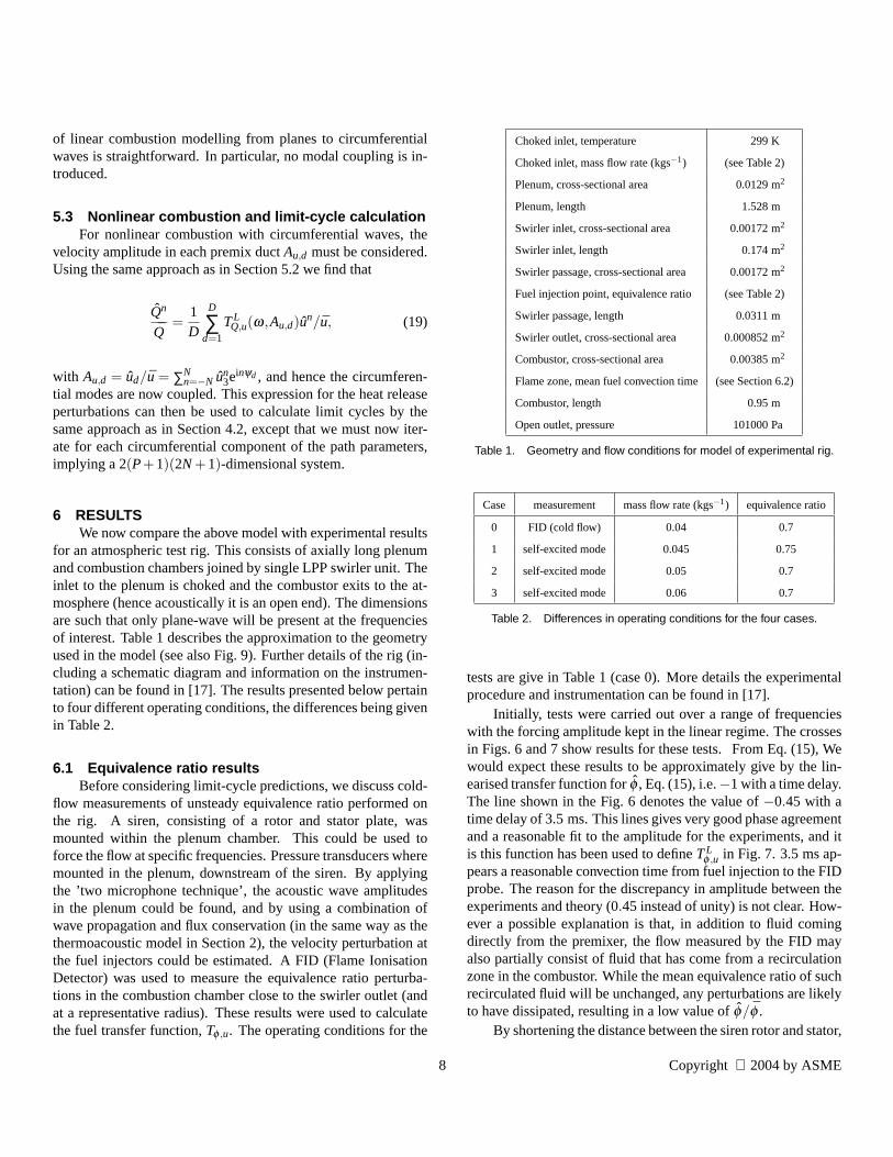
of the (mean) fuel convection time,τ, is not actually known forthe experimental rig. However, flame transfer function measure-ments suggestτ =5 ms for a mass flow of 0.04 kgs−1 [17]. Wewould expectτ to be approximately inversely proportional to themean velocity in the premixer and hence the inlet mass flow, i.e.τnew/τold = mold/mnew. Hence for each set of the operating con-ditions, we takeτ = 0.005× 0.04/m in the model. Althoughother rigs have demonstrated a single time delay [12] as in Eq.(13), this experimental set up demonstrates more complex dy-namics [17]. Nevertheless, to illustrate the method of predictionlimit-cycle amplitudes, we continue to use the simple descriptionof the flame responce recognising that it will lead to errors in thepredicted frequency. Figure 8 shows the linear modes found inthe complex frequency plane (up to 500 Hz). The crosses, circlesand pluses denotes operating conditions 1, 2 and 3, respectively.In each case there is a single mode that is highly unstable, therespective frequencies being at 222 Hz, 239 Hz and 269 Hz. Forcase 1 the frequency is within 10% of the experimental value.The other cases are less good, with case 3 particularly poor.

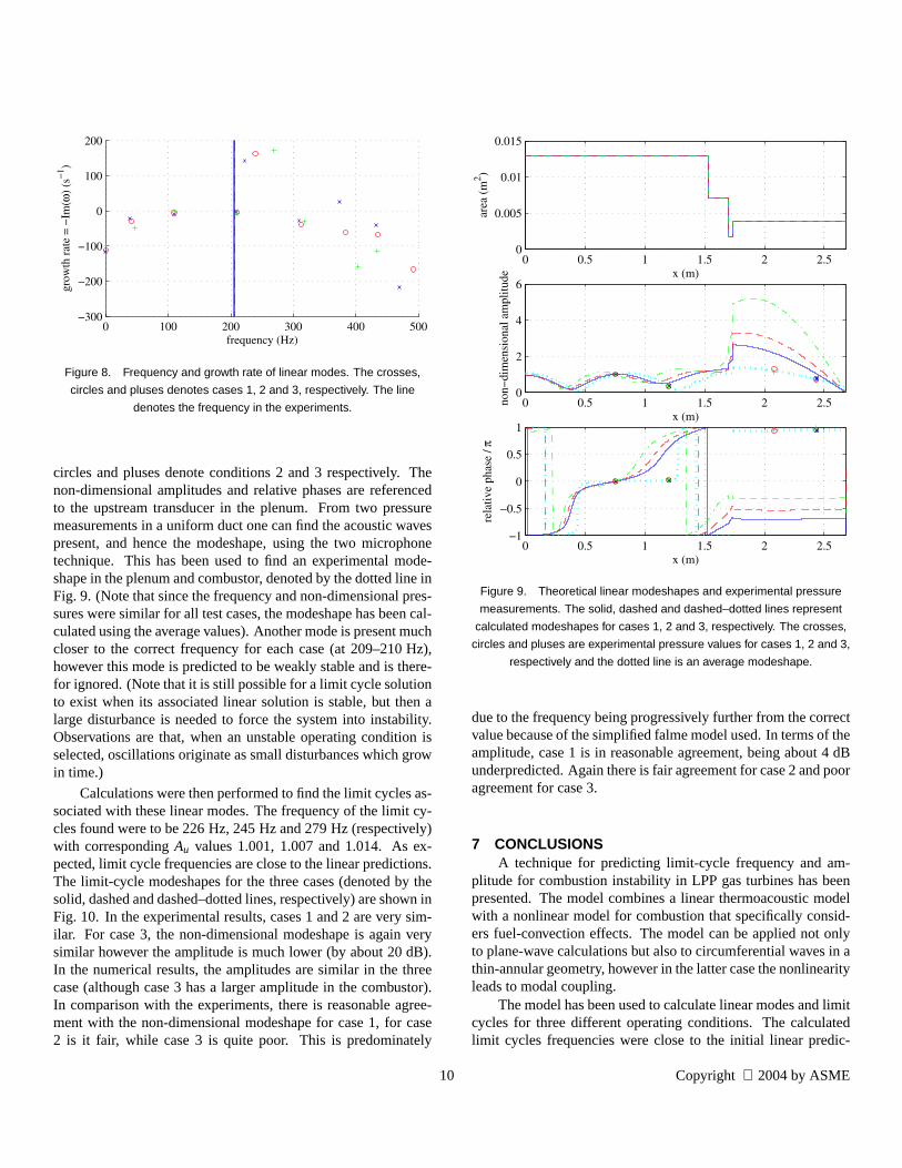
The modeshapes are plotted in Fig. 9 with the solid, dashedand dashed–dotted lines representing case 1, 2 and 3, respec-tively. These are compared with experimental measurementsfrom pressure transducers on the rig. (For conditions 2 and 3there were two transducers mounted in the combustor, whereasthere was only one for the tests at condition 1. Two plenum trans-ducers were present for all tests.) The FFT (Fast Fourier Trans-form) of the time signal from these transducer was taken and thevalue at the dominant frequency was found. The crosses in Fig.9 show these values for the three tests at condition 1, whereas the


0 100 200 300 400 500−300

−200

−100

0

100

200

frequency (Hz)

grow

th ra

te =

−Im

(ω) (

s−1)

Figure 8. Frequency and growth rate of linear modes. The crosses,

circles and pluses denotes cases 1, 2 and 3, respectively. The line

denotes the frequency in the experiments.

circles and pluses denote conditions 2 and 3 respectively. Thenon-dimensional amplitudes and relative phases are referencedto the upstream transducer in the plenum. From two pressuremeasurements in a uniform duct one can find the acoustic wavespresent, and hence the modeshape, using the two microphonetechnique. This has been used to find an experimental mode-shape in the plenum and combustor, denoted by the dotted line inFig. 9. (Note that since the frequency and non-dimensional pres-sures were similar for all test cases, the modeshape has been cal-culated using the average values). Another mode is present muchcloser to the correct frequency for each case (at 209–210 Hz),however this mode is predicted to be weakly stable and is there-for ignored. (Note that it is still possible for a limit cycle solutionto exist when its associated linear solution is stable, but then alarge disturbance is needed to force the system into instability.Observations are that, when an unstable operating condition isselected, oscillations originate as small disturbances which growin time.)

Calculations were then performed to find the limit cycles as-sociated with these linear modes. The frequency of the limit cy-cles found were to be 226 Hz, 245 Hz and 279 Hz (respectively)with correspondingAu values 1.001, 1.007 and 1.014. As ex-pected, limit cycle frequencies are close to the linear predictions.The limit-cycle modeshapes for the three cases (denoted by thesolid, dashed and dashed–dotted lines, respectively) are shown inFig. 10. In the experimental results, cases 1 and 2 are very sim-ilar. For case 3, the non-dimensional modeshape is again verysimilar however the amplitude is much lower (by about 20 dB).In the numerical results, the amplitudes are similar in the threecase (although case 3 has a larger amplitude in the combustor).In comparison with the experiments, there is reasonable agree-ment with the non-dimensional modeshape for case 1, for case2 is it fair, while case 3 is quite poor. This is predominately

0 0.5 1 1.5 2 2.50

2

4

6

x (m)

non−

dim

ensi

onal

am

plitu

de

0 0.5 1 1.5 2 2.5−1

−0.5

0

0.5

1

x (m)

rela

tive

phas

e / π

0 0.5 1 1.5 2 2.50

0.005

0.01

0.015

x (m)

area

(m2 )

Figure 9. Theoretical linear modeshapes and experimental pressure

measurements. The solid, dashed and dashed–dotted lines represent

calculated modeshapes for cases 1, 2 and 3, respectively. The crosses,

circles and pluses are experimental pressure values for cases 1, 2 and 3,

respectively and the dotted line is an average modeshape.

due to the frequency being progressively further from the correctvalue because of the simplified falme model used. In terms of theamplitude, case 1 is in reasonable agreement, being about 4 dBunderpredicted. Again there is fair agreement for case 2 and pooragreement for case 3.

7 CONCLUSIONSA technique for predicting limit-cycle frequency and am-

plitude for combustion instability in LPP gas turbines has beenpresented. The model combines a linear thermoacoustic modelwith a nonlinear model for combustion that specifically consid-ers fuel-convection effects. The model can be applied not onlyto plane-wave calculations but also to circumferential waves in athin-annular geometry, however in the latter case the nonlinearityleads to modal coupling.

The model has been used to calculate linear modes and limitcycles for three different operating conditions. The calculatedlimit cycles frequencies were close to the initial linear predic-


0 0.5 1 1.5 2 2.50

2000

4000

6000

8000

x (m)

ampl

itude

(Pa)

0 0.5 1 1.5 2 2.50

1

2

3

4

x (m)

non−

dim

ensi

onal

am

plitu

de

0 0.5 1 1.5 2 2.5−1

−0.5

0

0.5

1

x (m)

rela

tive

phas

e / π

Figure 10. Theoretical limit-cycle modeshapes and experimental

pressure measurements. The solid, dashed and dashed–dotted lines

represent calculated modeshapes for cases 1, 2 and 3, respectively. The

crosses, circles and pluses are experimental pressure values for cases

1, 2 and 3, respectively and the dotted line is an average modeshape.

tions. In comparison with experimental results, both the linearand nonlinear calculations were in reasonable agreement withthe first operating condition, fair agreement with the second andpoor agreement with the third. It is likely that this is becausethe frequency was progressively further from the correct valuedue to the simplicity of the linear flame model. Experimentalmeasurements of linear flame transfer functions [17] show that asimple time-delay model (Eq. (13)) is a poor representation of theflame behaviour on this particular rig. Better agreement is seenif, instead of assuming a single convection timeτ, one assumesa uniform spread of convection times (see also [26]). Such anassumption could be incorporated into the approach used in Sec-tion 3. Turbulent diffusion of equivalence ratio disturbances asthey are convected from the fuel injectors to the flame may alsobe an important effect, particularly at large amplitude. As well ascomparing limit-cycle predictions with experimental self-excitedmodes (as done in Section 6.2) an improved nonlinear flamemodel could be validated against heat-release measurements forhigh-amplitude forcing.

ACKNOWLEDGMENTThis work was funded by the European Commission

whose support is gratefully acknowledged. It is part of theGROWTH programme, research project ICLEAC: InstabilityControl of Low Emission Aero Engine Combustors (G4RD-CT2000-00215). The experimental results presented in this pa-per are from tests conducted Dr. Alex Riley, with assistance inthe FID tests from Dr. Karthik Balachandran (both of CambridgeUniversity Engineering Department).

REFERENCES[1] C. O. Paschereit, B. Schuermans, W. Polifke and O. Matt-

son, 2002, “Measurement of transfer matrices and sourceterms of premixed flames”, J. Eng. Gas. Turbines Power,124, pp. 239–247.

[2] U. Kruger, J. Hurens, S. Hoffmann, W. Krebs and D. Bohn,1999, “Prediction of thermoacoustic instabilities with focuson the dynamic flame behavior for the 3A-series gas turbineof Siemens KWU”, ASME Paper 99-GT-111.

[3] U. Kruger, J. Hurens, S. Hoffmann, W. Krebs, P. Flohr andD. Bohn, 2000, “Prediction and measurement of thermoa-coustic improvements in gas turbines with annular combus-tion systems”, ASME Paper 2000-GT-0095.

[4] G. C. Hsiao, R. P. Pandalai, H. S. Hura and H. C. Mon-gia, 1998, “Combustion dynamic modeling for gas turbineengines”, AIAA Paper 98-3380.

[5] G. C. Hsiao, R. P. Pandalai, H. S. Hura and H. C. Mon-gia, 1998, “Investigation of combustion dynamics in dry-low-emission (DLE) gas turbine engines”, AIAA Paper 98-3381.

[6] A. P. Dowling and S. R. Stow, 2003, “Modal analysis of gasturbine combustor acoustics”, J. Propul. Power,19(5), pp.751–764.

[7] F. E. C. Culick, 1971, “Non-linear growth and limiting am-plitude of acoustic oscillations in combustion chambers”,Combust. Sci. Technol.,3(1), pp. 1–16.

[8] F. E. C. Culick, 1989, “Combustion instabilities in liquid-fueled propulsion systems — an overview”, AGARD Con-ference Proceedings No. 450, Paper 1.

[9] A. A. Peracchio and W. M. Proscia, 1999, “Nonlinearheat-release/acoustic model for thermoacoustic instabilityin lean premixed combustors”, J. Eng. Gas. Turbines Power,121(3).

[10] C. Pankiewitz and T. Sattelmayer, 2003, “Time domainsimulation of combustion instabilities in annular combus-tors”, J. Eng. Gas. Turbines Power,125(3), pp. 677–685.

[11] B. Schuermans, V. Bellucci and Paschereit C. O., 2003,“Thermoacoustic modeling and control of multi burnercombustion systems”, ASME Paper GT2003-38688.

[12] G. A. Richards and M. C. Janus, 1998, “Characterization of


oscillations during premix gas turbine combustion”, J. Eng.Gas. Turbines Power,120(2), pp. 294–302.

[13] T. Lieuwen and B. Zinn, 1998, “The role of equivalenceratio oscillations in driving combustion instabilities in lowNOx gas turbines”, 27th International Symposium on Com-bustion.

[14] A. P. Dowling, 1999, “A kinematic model of a ductedflame”, J. Fluid Mech.,394, pp. 51–72.

[15] S. R. Stow and A. P. Dowling, 2003, “Modelling of cir-cumferential modal coupling due to Helmholtz resonators”,ASME Paper GT2003-38168.

[16] S. R. Stow and A. P. Dowling, 2001, “Thermoacoustic os-cillations in an annular combustor”, ASME Paper 2001-GT-0037.

[17] C. A. Armitage, A. J. Riley, R. S. Cant, A. P. Dowlingand S. R. Stow, 2004, “Flame transfer function for swirledLPP combustion from experiment and CFD”, ASME PaperGT2004-52830.

[18] T. Sattelmayer, 2000, “Influence of the combustor aerody-namics on combustion instabilities from equivalence ratiofluctuations”, ASME Paper 2000-GT-0082.

[19] S. Hubbard and A. P. Dowling, 1998, “Acoustic instabilitiesin premix burners”, AIAA Paper 98-2272.

[20] A. P. Dowling, 1999, “Thermoacoustic instability”, 6th In-ternational Congress on Sound and Vibration.

[21] W. Polifke, C. O. Paschereit and K. Dobbeling, 1999, “Sup-pression of combustion instabilities through destructive in-terference of acoustic and entropy waves”, 6th InternationalCongress on Sound and Vibration.

[22] T. Lieuwen and Y. Neumeier, 2003, “Nonlinear pressure-heat release transfer function measurements in a premixedcombustor”, P. Combust. Inst.,19(5), pp. 765–781.

[23] B. O. Aylooa, R. Balachandran, A. P. Dowling, J. H. Frank,C. F. Kaminski and E. Mastorakos, 2004, “Flame transferfunction measurements in bluff-body stabilised turbulentpremixed flames”, submitted to 30th International Sympo-sium on Combustion.

[24] S. Akamatsu and A. P. Dowling, 2001, “Three dimen-sional thermoacoustic oscillation in an premix combustor”,ASME Paper 2001-GT-0034.

[25] S. Evesque and W. Polifke, 2002, “Low-order acousticmodelling for annular combustors: validation and inclusionof modal coupling”, ASME Paper GT-2002-30064.

[26] W. S. Cheung, G. J. M. Sims, R. W. Copplestone, J. R.Tilston, C. W. Wilson, S. R. Stow and A. P. Dowling, 2003,“Measurement and analysis of flame transfer function in asector combustor under high pressure conditions”, ASMEPaper GT2003-38219.


low-order modelling of thermoacoutic limit cycles - iwr

Documents