Massachusetts Low‐Income 

Multifamily Initiative  

Impact Evaluation October 2015 

 

Prepared for 

The Electric and Gas Program Administrators of Massachusetts 

Part of the Residential Evaluation Program Area 

 

 

 

 

 

 

 

 

 

 

 

 

 

 

 

 

 

This page left blank. 

 

 

 

 

 

 

 

 

 

 

 

 

 

 

 

Prepared by: 

Scott Reeves 

Arlis Reynolds 

Matei Perussi 

Tim Murray 

Robert Lamoureux 

M. Sami Khawaja, Ph.D. 

 

Cadmus 

 

 

 

 

 

 

 

 

 

 

 

 

 

 

 

 

 

 

 

 

 

This page left blank. 

 

 

i 

Table of Contents Acronym Glossary ........................................................................................................................................ vi 

Executive Summary ....................................................................................................................................... 8 

Objectives ............................................................................................................................................... 8 

Methods ................................................................................................................................................. 8 

Results .................................................................................................................................................... 9 

Study Considerations ............................................................................................................................ 11 

Introduction ................................................................................................................................................ 14 

Overview ............................................................................................................................................... 14 

Evaluation Objectives ........................................................................................................................... 15 

Report Organization ............................................................................................................................. 17 

Task 1. Engineering Analysis and Literature Review ................................................................................... 18 

Methods ............................................................................................................................................... 18 

Results .................................................................................................................................................. 19 

Heating System Replacement Baseline ................................................................................................ 26 

Task 2. Natural Gas Billing Analysis ............................................................................................................. 27 

Methods ............................................................................................................................................... 27 

Results .................................................................................................................................................. 32 

Task 3. Common Area Lighting ................................................................................................................... 39 

Methods ............................................................................................................................................... 39 

Results .................................................................................................................................................. 45 

Task 4. On‐Site Verification and Measure Analysis ..................................................................................... 47 

Showerheads and Aerators .................................................................................................................. 47 

Air Conditioning Equipment ................................................................................................................. 49 

Task 5. Assessment of Secondary Impacts .................................................................................................. 51 

Water Savings ....................................................................................................................................... 51 

Interactive Cooling Impacts .................................................................................................................. 54 

Appendix A. Summary of Deemed Savings Values ..................................................................................... 56 

Appendix B. Billing Analysis Model Specification ....................................................................................... 58 

PRISM Model ........................................................................................................................................ 58 

Combined Fixed‐Effects Model ............................................................................................................ 58 

 

ii 

Appendix C. References .............................................................................................................................. 60 

Appendix D. Billing Analysis – Supplemental Results ................................................................................. 62 

Measure‐Level Modeling ...................................................................................................................... 62 

 

 

 

iii 

List of Tables Table 1. LIMF Gross Natural Gas Participant Savings by PA and Overall ...................................................... 9 

Table 2. LIMF Gross Realization Rate Summary by PA and Overall ............................................................ 10 

Table 3. Common Area Lighting Realization Rates ..................................................................................... 10 

Table 4. Assessment of Secondary Impacts ................................................................................................ 11 

Table 5. Program Administrators: Natural Gas and Electric Support ......................................................... 14 

Table 6. LIMF Impact Evaluation Research Objectives ............................................................................... 16 

Table 7. Deemed Savings—Electric Measures ............................................................................................ 21 

Table 8. TLC Kit Measures Currently Offered in the LIMF Initiative ........................................................... 25 

Table 9. Deemed Savings – Natural Gas Measures ..................................................................................... 25 

Table 10. Final Participant Group Attrition Per PA and Overall .................................................................. 30 

Table 11. Overall State‐Level Participant Group Attrition Detail* .............................................................. 31 

Table 12. Comparison of Measure Distribution Between Sample and Population, per PA ....................... 32 

Table 13. LIMF Gross Natural Gas Participant Savings Per PA and Overall ................................................ 33 

Table 14. LIMF Gross Realization Rate Summary Per PA and Overall ........................................................ 34 

Table 15. LIMF Gross Natural Gas Participant Savings Per Claimed Savings Type ..................................... 37 

Table 16. LIMF Lighting Projects and Savings by PA (PY 2014) ................................................................... 39 

Table 17. Definition of Common Area Lighting Population ........................................................................ 40 

Table 18. Number of Common Area Lighting Sample of Projects Visited and PA Per Strata ..................... 41 

Table 19. Percentage of Annual kWh Savings by Population and Projects Visited Per Strata ................... 41 

Table 20. Common Area Lighting Metering Equipment ............................................................................. 42 

Table 21. Common Area Metering Equipment ........................................................................................... 45 

Table 22. Common Area Lighting Deemed Savings Values ......................................................................... 45 

Table 23. Faucet Aerator and Showerhead Installations Per Project Site .................................................. 48 

Table 24. ISR Calculation for Faucet Aerators and Showerheads ............................................................... 49 

 

iv 

Table 25. Type of Air Conditioning Equipment Observed On site .............................................................. 50 

Table 26. Faucet Aerator Water Saving Calculation Inputs ........................................................................ 52 

Table 27. Average Faucet Aerator Water Saving ........................................................................................ 52 

Table 28. Showerhead Savings Calculation Inputs ...................................................................................... 53 

Table 29. Inputs to Calculate Weatherization Cooling Savings of RAC Units ............................................. 55 

Table 30. Typical Weatherization Savings ................................................................................................... 55 

Table 31. Measure Installation Overlap (Percent of Units) ........................................................................ 62 

Table 32. Measure‐Level Gas Savings Impacts ........................................................................................... 63 

 

   

 

v 

List of Figures Figure 1. Annual LIMF Electric and Gas Energy Savings by PA (PY 2014)* ................................................. 15 

Figure 2. Model vs. Ex Ante Gross Savings as a Percentage of PRENAC Per PA.......................................... 35 

Figure 3. Model vs. Ex Ante Gross Savings as a Percentage of PRENAC Per Usage Quartile ...................... 36 

Figure 4. Model vs. Ex Ante Gross Savings as a Percentage of PRENAC ..................................................... 36 

Figure 5. Comparison of Evaluated Savings as a Percentage of PRENAC by Program ................................ 37 

Figure 6. Comparison of Evaluated Absolute Savings by Program ............................................................. 38 

Figure 7. Cumulative Savings by Number of Projects ................................................................................. 40 

Figure 8. Common Area light Metering Raw Data Sample (Bi‐Level) ......................................................... 42 

Figure 9. Sample Weekday Common Area Light Runtime Profile (Bi‐Level) .............................................. 43 

Figure 10. Stairway HOU Distribution High Level (Bi‐Level) ....................................................................... 43 

Figure 11. Hallway HOU Distribution at High Level (Bi‐Level) .................................................................... 44 

Figure 12. Distribution of Observed Faucet Aerators and Showerheads by Rated Flow Rate ................... 48 

Figure 13. Deemed Savings Summary ‐ Electric .......................................................................................... 56 

Figure 14. Deemed Savings Summary ‐ Gas ................................................................................................ 57 

 

 

vi 

Acronym Glossary 

Acronym  Definition 

ABCD  Action for Boston Community Development, Inc. 

AC  Air Conditioning 

ADC  Average Daily Consumption 

AVGCDD  Average Daily Cooling Degree Days 

AVGHDD  Average Daily Heating Degree Days 

BA  Bathroom Aerator 

BCR  Benefit Cost Ratio 

Btu  British Thermal Unit 

CAC  Central Air Conditioner 

CFL  Compact Fluorescent 

CLC  Cape Light Compact 

DSW  Deemed Savings Workbook 

EEAC  Massachusetts Energy Efficiency Advisory Council 

EER  Energy Efficiency Ratio 

EFLH  Equivalent Full Load Hours 

EISA  Energy Independence and Security Act 

EMS  Energy Management System 

GPM  Gallons per Minute 

HAC  Housing Assistance Corporation 

HDD  Heating Degree Day 

HEATNAC  Heating Normalized Annual Consumption 

HOU  Hours of Use 

ISR  In Service Rate 

KA  Kitchen Aerators 

kWh  Kilowatt Hour 

LEAN  Low Income Energy Affordability Network 

LED  Light Emitting Diode 

LIMF  Low Income Multifamily 

LRHDD  Annual long‐term Heating Degree Days 

MOC  Montachusetts Opportunity Council 

NAC  Normalized Annual Consumption 

NOAA  National Oceanic and Atmospheric Administration 

PA  Program Administrator 

PRENAC  Pre Period Normalized Annual Consumption 

PRISM  Princeton Scorekeeping Method 

PY  Program Year 

RAC  Room Air Conditioner 

TMY  Typical Meteorological Year 

TRM  Technical Reference Manual 

VFD  Variable Frequency Drive 

 

vii 

 

 

 

 

 

 

 

 

 

 

 

 

This page left blank. 

 

8 

Executive Summary 

The Massachusetts Low‐Income Multifamily (LIMF) Retrofit Initiative provides technical, financial, and 

project management support to implement electric and natural gas efficiency upgrades at eligible 

buildings. This report describes the objectives, methods, and results of the first impact evaluation of the 

LIMF Initiative.  

Objectives Through a series of workshops held in 2014, the LIMF Stakeholders—including Program Administrators 

(PAs), evaluators, the low‐income advocacy agencies, Energy Efficiency Advisory Council consultants, 

and other initiative contractors—examined initiative activities and determined evaluation objectives. 

Based on broader objectives of verifying energy impacts, improving transparency and consistency in 

savings estimation methods, the evaluation team defined five key evaluation tasks:  

1. Engineering analysis and literature review. Develop a set of statewide savings estimates for 

non‐custom measures to improve transparency and consistency across the state. 

2. Natural gas billing analysis. Verify the impacts of the natural gas initiative, which is dominated 

by weatherization, heating, and water heating measures.  

3. Common area lighting analysis. Verify the impacts of common area lighting measures, which—

combined with in‐unit lighting measures—dominate the electric initiative. 

4. On‐site verification and measure analysis. Leverage data collection efforts to verify installation 

and collect data for non‐lighting measures.  

5. Assessment of secondary impacts. Examine secondary energy and water impacts for existing 

initiative measures.  

Methods Between January 2015 and August 2015, the evaluation team examined tracking and TRM data, 

collected and analyzed billing data, and performed site visits with lighting time‐of‐use (TOU) metering to 

complete the tasks outlined above. Specifically, the team:  

1. Developed a Deemed Savings Workbook (DSW) in Microsoft Excel® that presents proposed 

statewide savings estimate for non‐custom measures, including comprehensive information 

about algorithms, assumptions, and sources with live calculations.  

2. Performed a billing analysis to estimate the impacts of program year (PY) 2012 and PY 2013 

natural gas projects.  

3. Conducted on‐site verification and TOU metering for a sample of 56 electric projects from PY 

2014 to estimate a realization rate for common area lighting measures.  

4. Collected and analyzed information about energy‐efficient showerheads, aerators, and building 

cooling and heating equipment at the projects in the common area lighting analysis sample. 

 

9 

5. Reviewed tracking and secondary data to update water savings values and estimate interactive 

impacts of weatherization measures on cooling energy.  

The evaluation team completed analysis for all tasks and presented results to the LIMF Stakeholder 

group on August 24, 2015.  

Results This impact evaluation provides the following results for the LIMF electric and natural gas initiatives:  

1. The DSW provides a table of statewide deemed savings values for non‐custom measures to 

improve transparency, consistency, and accuracy across the PA initiatives. The workbook is a 

Microsoft Excel® workbook and outlines all calculations, assumptions, and sources used to 

quantify the deemed savings values. Appendix A (Summary of Deemed Savings Values) shows 

the summary tables for electric and natural gas measures.  

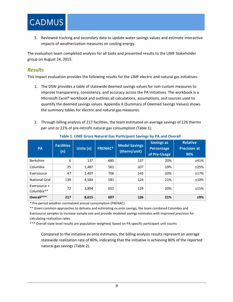
 2. Through billing analysis of 217 facilities, the team estimated an average savings of 126 therms 

per unit or 21% of pre‐retrofit natural gas consumption (Table 1).  

Table 1. LIMF Gross Natural Gas Participant Savings by PA and Overall 

PA  Facilities 

(n) Units (n)  PRENAC* 

Model Savings 

(therm/unit) 

Savings as 

Percentage 

of Pre‐Usage 

Relative 

Precision at 

90% 

Berkshire  6  137  685 137 20%  ±41%

Columbia  25  1,487  561 107 19%  ±25%

Eversource  47  2,407  706 143 20%  ±17%

National Grid  139  4,584  581 124 21%  ±10%

Eversource + 

Columbia** 72  3,894  651 129 20%  ±15%

Overall***  217  8,615  607 126 21%  ±9%

* Pre‐period weather‐normalized annual consumption (PRENAC) 

** Given common approaches to delivery and estimating ex ante savings, the team combined Columbia and 

Eversource samples to increase sample size and provide modeled savings estimates with improved precision for 

calculating realization rates.  

*** Overall state‐level results are population‐weighted, based on PA‐specific participant unit counts 

 Compared to the initiative ex ante estimates, the billing analysis results represent an average 

statewide realization rate of 80%, indicating that the initiative is achieving 80% of the reported 

natural gas savings (Table 2).  

 

10 

Table 2. LIMF Gross Realization Rate Summary by PA and Overall 

PA* Model Savings 

(therm) 

Reported Ex Ante 

Savings (therm) 

Realization 

Rate 

Ex Ante Savings as % 

of Pre‐Usage 

Berkshire  137  241 57% 35%

Columbia  107  131 82% 23%

Eversource  143  136 105% 19%

National Grid  124  166 75% 29%

Eversource + 

Columbia** 129  134 96% 21%

Overall***  126  158 80% 26%

* Due to few participants and lack of available consumption data, this analysis excluded Liberty and Unitil. 

** Given common approaches to delivery and estimating ex ante savings, the team combined Columbia and 

Eversource samples to increase sample size and provide modeled savings estimates with improved precision for 

calculating realization rates. 

 *** Overall state‐level results are population‐weighted, based on PA‐specific participant unit counts 

 The majority of projects that received natural gas efficiency measures to reduce heating 

consumption also received efficient lighting measures. The lighting upgrade increases heating 

loads because the more efficient lighting contributes less waste heat into occupied spaces. Gas 

billing analysis, by its nature, does not separate out these two effects and thus underestimates 

the savings achieved by the gas saving measures. Separating out the lighting interactive effects 

on the heating load should increase the realization rate to somewhere between 83% and 89%. 

3. The team estimated a statewide realization rate of 97% for common area lighting measures, 

verifying that auditors are accurately estimating annual energy savings. Table 3 lists the 

statewide realization rate and relative precision at a 90% confidence level.  

Table 3. Common Area Lighting Realization Rates 

PA  Realization Rate Relative Precision 

at 90% Confidence 

National Grid  101% ±8%

Eversource  96% ±2%

Statewide  97% ±3%

 4. Through inspection of showerheads and faucets within 20 apartment units, the team confirmed 

that all showerheads were below the 2.5‐gallon‐per‐minute maximum threshold and most 

faucet aerators were below the 1.5‐gallon‐per‐minute threshold.  

5. Through documentation of the cooling type at all 56 projects in the common area lighting 

sample, the team estimated that 89% of facilities use window air‐conditioning as the primary 

cooling equipment.  

 

11 

6. Finally, through literature review and examination of the primary data collected in this study, 

the evaluation team estimated the deemed values in Table 4. 

Table 4. Assessment of Secondary Impacts 

Savings Parameter  Annual Value 

Faucet Aerator Water Savings – Bathroom*  416 gallons 

Faucet Aerator Water Savings – Kitchen*  1,133 gallons 

Faucet Aerator Water Savings – Average*  708 gallons 

Showerhead Water Savings  1,759 gallons 

Clothes Washer Water Savings  6,948 gallons 

Cooling Savings (Weatherization)  22 kWh 

* The average aerator value is a weighted average based on expected allocation of installed aerators between kitchens and bathrooms. PAs should use the average value for faucet aerators only if they do not track location of the installation aerator equipment.  

 

Study Considerations Based on the research findings, the team has identified several study considerations to improve LIMF 

Initiative performance and operations. 

Improve Initiative Tracking 

The following improvements to the LIMF Initiative tracking systems and data will increase statewide 

consistency and reporting, facilitate future evaluations, and provide valuable data for future TRM 

updates and implementation strategies: 

Standardize measure descriptions and measure categories across all PA datasets. For 

deemed measures, adopt the proposed naming convention outlined in Appendix A 

(Summary of Deemed Savings Values). 

Define a project unit (such as apartment unit vs. common area, building, or facility) and 

provide unique identifiers that easily allow for associated measure installations and other 

project details across these various levels. 

Include additional fields using standardized conventions across all PA datasets such as 

building type (e.g., row house, high rise), presence of common areas, and meter 

configuration (e.g., master meter plus in‐unit meters, master meter only). 

For lighting measures, track the space type for each installed lighting measure using a table 

of standard space type options. 

For lighting measures, improve documentation of replaced (i.e., baseline) equipment by 

requiring auditors to photograph at least one example of baseline and installed fixtures. 

For bi‐level lighting installations, track the high and low fixture wattage and estimated HOU 

at the high and low wattage setting for each installed measure.  

 

12 

Review Ex Ante Savings Assumptions for Natural Gas Measures  

While realization rates overall and by PA are reasonable, some issues remain with ex ante savings. The 

estimated actual savings are consistent, reasonable, and accurate (high levels of precision in most 

cases). The PAs achieved between a 19% and 21% reduction in usage. Yet, their ex ante values ranged 

from 18% to 35%. Realization rates less than 100% may be driven by persistence or quality of measure 

installations, or through overestimation of installed savings. One factor that may have a larger impact on 

planning estimates for multifamily initiatives is how savings account for vacancies and changes in 

occupancy. Another important factor to consider for initiatives that similarly deliver holistic services is 

measure interactive effects—including the impact of efficient lighting on achieving gas savings 

attributed to reduced heating load. In most cases, initiatives that rely on deemed values tend to have 

lower realization rates, while those that take into account conditions and consumption levels at each 

site tend to have higher realization rates. The team recommends a review of ex ante savings 

assumptions to understand and account for how issues like vacancies and measure interactions (e.g., 

lighting) are addressed. 

Application of Realization Rates for Prospective Program Planning 

Ideally, this analysis would have produced reliable PA‐specific realization rates that reflect the 

uniqueness of the customers and delivery mechanism. Unfortunately, as mentioned above, that was not 

possible for smaller PAs. As a result, the team suggests prospectively using realization rates as follows: 

Eversource use their own realization rate of 105% 

National Grid should apply their own realization rate of 75%. National Grid was the only PA that used deemed values instead of simulation modeling. 

Other PAs using the same delivery agency and approach to estimating ex ante savings (i.e., Columbia, Liberty, Unitil) should use a realization rate based on combined analysis sample of Columbia and Eversource at 96%.  

Berkshire should use the statewide realization rate of 80%. 

This recommendation should be contingent upon implementation agencies, forward looking, providing 

documentation to help clarify some of the differences in average ex ante savings across PA analysis 

samples, as mentioned above. The provision of full documentation of ex ante calculations will be 

important to ensure steps are taken to review and refine this process, acknowledging improvements to 

justify application of these prospective realization rates. Furthermore, we suggest additional safeguards 

included in the process for verifying and reporting claimed savings estimates, including checks against 

pre‐consumption per project, with explanation provided in cases where expected percent savings occurs 

over a specified threshold (e.g., 30%).  

Examine Factors Driving High and Low Savings 

The Princeton Scorekeeping Method (PRISM) analysis provides facility‐specific changes in usage, 

allowing identification of a sample of projects that demonstrated extremes in high and low initiative 

savings. As a next step, the team recommends performing an on‐site assessment for a sample of 

projects identified through this analysis to provide a deeper understanding of factors driving high and 

 

13 

low savings. For example, the study might assess projects with similar building sizes and measure mixes, 

but with realization rates on opposite ends in order to investigate which key factors may have 

contributed to such differences in savings.  

Collect Data to Assess Appropriate Baseline for Heating System Upgrade Measures 

A May 2014 memorandum documented key differences in the baseline assumptions used by PAs to 

estimate ex ante savings for gas heating system upgrades.1 While collection of key data elements to 

inform baseline is an important first step, there is concurrent research planned in Massachusetts to 

consider an approach to baseline assessment that will be aimed at broader statewide applicability. 

Based on nuances surrounding how conditions for early replacement are characterized and verified, 

there may be future guidance that refines data requirements and/or methodology for defining the 

appropriate savings baseline. In particular, low income‐specific conditions need to be explicitly 

considered in the data collection effort (e.g., boilers). 

 

                                                            

1   Memorandum: Baseline Assumptions for Heating Replacements in the Low Income Multifamily Program.     May 2014. 

 

14 

Introduction 

This report, developed for the Massachusetts Low‐Income Multifamily (LIMF) Retrofit Initiative 

stakeholders, describes the objectives, methods, and results from the first impact evaluation of the LIMF 

Retrofit Initiative. The team combined engineering analysis and tracking data review, billing analysis, 

direct measurement, and on‐site verification to achieve the objectives agreed upon by the LIMF 

stakeholders.  

Overview The LIMF Initiative provides technical, financial, and project management support to implement natural 

gas and electric efficiency upgrades at eligible residential multifamily buildings. Eligible properties 

contain five or more units of which at least 50% of the occupants earn 60% or less of the area median 

income.  

Through the LIMF implementation contractors, who oversee most of the initiative processes, the 

Program Administrators (PAs) provide full funding (i.e., 100% of the equipment and installation costs) to 

identify and implement cost‐effective electric and natural gas efficiency measures. As shown in Table 5, 

six of the Massachusetts PAs offer the initiative to reduce natural gas consumption, and four PAs offer 

measures to reduce electricity consumption.  

Table 5. Program Administrators: Natural Gas and Electric Support 

Program Administrator  Natural Gas  Electric 

Berkshire Gas (Berkshire)  ✓    

Cape Light Compact (CLC)     ✓ 

Columbia Gas of Massachusetts (Columbia Gas)  ✓    

Liberty Utilities (Liberty)  ✓    

National Grid  ✓  ✓ 

Eversource Energy (Eversource; formerly Northeast Utilities)  ✓  ✓ 

Unitil  ✓  ✓ 

 Each PA uses an implementation contractor, or lead agency that is part of the Massachusetts Low‐

income Energy Affordability Network (LEAN), to administer most aspects of the initiative. The lead 

agencies perform or oversee site inspections and energy audits, measure screening, measure 

implementation, and final inspections. One lead agency, Action for Boston Community Development, 

Inc. (ABCD), manages the statewide intake process including the leanmultifamily.org website for 

recruiting participants and performing the initial screening for basic site qualification. 

ABCD manages the implementation of measures for Columbia Gas and Eversource. Additional lead 

agencies support the efforts of the other PAs, who may recruit participants or obtain them from through 

ABCD. The lead agencies include Action, Inc., (Action) for National Grid; the Housing Assistance 

Corporation (HAC) for CLC; Community Action Inc. (CAI) for Berkshire Gas; Citizens for Citizens, Inc., for 

 

15 

Liberty Gas; and the Montachusett Opportunity Council (MOC) for Unitil. Third‐party vendors participate 

in a regular and competitive bidding process to earn contracts for installing the approved measures. 

For each installed measure, the PAs claim energy and demand savings based on a deemed number, 

standard algorithm, or custom calculation (including simulation modeling). A deemed number is a single 

predetermined savings value based on assumptions supported by previous evaluations or engineering 

analysis. A standard algorithm is a calculation that involves fixed assumptions with one or more project‐

specific input. Custom calculations are typically performed using computer simulations based on site‐

specific information and engineering assumptions.  

The evaluation team analyzed reported savings data for the Program Year 2014 LIMF Initiative to assess 

savings by PA. Figure 1 shows the annual electric and gas energy savings claimed by each PA for program 

year (PY) 2014.  

Figure 1. Annual LIMF Electric and Gas Energy Savings by PA (PY 2014)*  

*Source: Mass Save. Performance Details: 2014 Summary Report. Available online: 

http://masssavedata.com/Public/PerformanceDetails.aspx .  

 National Grid and Eversource contributed the majority of the statewide gas and electric energy savings, 

respectively. 

Evaluation Objectives To determine the study objectives, the residential evaluation team (evaluation team or team) engaged 

LIMF Initiative stakeholders from the PAs, LEAN, lead agencies, EEAC, and implementation contractors. 

 

16 

The team held multiple workshops to discuss evaluation needs and determine areas of focus for this 

evaluation.  

The first stakeholder workshop, held on July 17, 2014, was principally for fact‐finding purposes. It 

yielded essential information about the operation of the initiative as a whole and enabled the team to 

identify key areas of interest. Following the meeting, the team held interviews with representatives 

from the two largest lead agencies—ABCD and Action—and with each PA to discuss their specific 

evaluation goals, understand their methods for data tacking and savings estimation, and to learn how 

they operate within the statewide initiative.  

The evaluation team also reviewed tracking data obtained directly from the PAs including benefit/cost 

ratio (BCR) model worksheets and detailed per‐site, per‐measure tracking data. The team compared the 

per‐measure data to various editions of the Massachusetts Technical Reference Manual (TRM) and to 

the savings values reported for the PY 2013 LIMF Initiative.  

The team compiled its findings from the stakeholder interviews and tracking data review into a technical 

review memo and presented the results in the second stakeholder workshop held on October 23, 2014. 

In the memo, the evaluation team proposed research activities that address the stakeholders’ 

evaluation goals. The memo focused on measures that represented the most savings and that had the 

greatest uncertainty in savings estimation.  

During the final stakeholder workshop, held on December 1, 2014, the stakeholders and evaluation 

team agreed upon a defined set of research objectives. Table 6 shows the final list of evaluation 

objectives and the approach to achieve each objective. 

Table 6. LIMF Impact Evaluation Research Objectives 

Research Objective  Approach

1. Verify energy impacts achieved by the LIMF 

Initiative* 

Ensure savings methods and assumption are clearly 

documented 

2. Improve Transparency of Savings 

Estimation Methods 

Ensure savings methods and assumption are clearly 

documented 

3. Improve Consistency in Savings Estimation, 

Tracking, and Reporting 

Provide recommendations to improve consistency in estimated 

savings values, data tracking methods, and reported savings. 

4. Highlight Initiative Achievements Document verified energy and cost savings for LIMF customers

Estimate non‐energy benefits

* The impact evaluation focused on energy impacts only; it did not include demand impacts. 

 Following the final stakeholder workshop, the evaluation team developed a detailed evaluation plan based on the objectives in the table above and specific evaluation tasks outlined to achieve each objective.  

 

17 

Report Organization This report is organized into the five research tasks determined through stakeholder meetings:  

1. Engineering analysis and literature review. For measures not requiring primary data collection, 

the evaluation team used existing literature and engineering analysis to determine the best 

method for estimating savings. This effort included these activities:  

Defining a common set of naming conventions to standardize the granularity of data and to 

improve transparency;  

Recommending the best approach to estimate savings; and 

When applicable, selecting the most appropriate deemed values to maximize consistency. 

2. Billing analysis. The team estimated savings using a combination of regression models. The 

team used the participants’ billing and tracking data to model monthly facility‐level gas 

consumption.  

3. Metering study. The team metered lighting hours of use (HOU) for a variety of common area 

space types to determine realization rates relative to ex ante energy savings.  

4. On‐site verification and measure analysis. The team conducted on‐site visits to verify installed 

equipment and operating parameters.  

5. Assessment of secondary savings. The team explored project benefits beyond primary fuel 

conservation. Specifically, the team reviewed the estimation of water savings and the impact of 

weatherization measures on cooling season energy consumption. 

 

18 

Task 1. Engineering Analysis and Literature Review 

Through the initial technical review process, the evaluation team analyzed savings data for the PY 2013 

LIMF Initiative.2 This activity highlighted three opportunities for increased transparency and consistency: 

Measure naming convention. In many cases, PAs used different names and level of detail to 

track measures, making it difficult to make measure‐level comparisons across PA initiatives. For 

example, some PAs separate common area lighting from in‐unit lighting, while others combine 

them into a single category.  

Savings calculation methods. In some cases, PAs use different methods to estimate savings. For 

example, one PA may use a deemed value while another uses a calculation.3 

Deemed values and assumptions. PAs may use different deemed values to estimate savings for 

the same measure. These values may or may not be applicable to the LIMF Initiative. 

To improve transparency and consistency in tracking, estimating, and reporting ex ante savings 

estimates for non‐custom4 measures, the evaluation team developed the LIMF Deemed Savings 

Workbook (DSW). The DSW presents a set of statewide deemed savings values and provides 

comprehensive documentation of the methods and assumptions used to estimate those values.  

The team also reviewed inconsistent baseline assumptions used by PAs to estimate savings from heating 

system upgrades and recommended data collection to support a dual baseline approach in the future.  

This discussion is summarized at the end of this chapter and documented in a May 2014 memorandum.5 

Methods The PAs provided a new statewide measure list (developed by the PA common assumptions working 

group) noting that all PAs would use the same list of measure names for future LIMF activities. This 

statewide measure list solved the inconsistency in measure naming conventions. 

                                                            

2   Cadmus. MA LIMF Technical Review Summary of Findings Memo. Prepared for the Electric and Gas Program Administrators of Massachusetts. 2014. 

3   Certain PAs use deemed values to estimate savings from every measure. The evaluation team does not propose that they change their approach, but it has identified opportunities for greater standardization among the PAs that do use the algorithm approach to estimate savings.  

4   Non‐custom measures use standard algorithms and assumptions to estimate savings. Savings estimates may be deemed (e.g., a single savings value per measure) or deemed‐calculated (e.g., a deemed algorithm with one or more project‐specific inputs). 

5   Memorandum: Baseline Assumptions for Heating Replacements in the Low Income Multifamily Program. May 2014. 

 

19 

To address differences in savings estimation methods and values, the team: 

Reviewed the Massachusetts TRM and PA tracking data and conducted stakeholder interviews 

to document existing savings estimation methods and values used by each PA for each measure.  

Examined all source material cited in the TRM to assess the validity of each assumption.  

o In most cases, the data were not specific to LIMF buildings. Values were often based on 

studies focused on either low‐income single‐family or standard‐income multifamily 

buildings.  

Compared calculation methods and assumptions across measures to identify opportunities to 

improve consistency among savings assumptions for the overall initiative.  

Selected appropriate savings estimation methods and assumptions for each measure taking into 

account recent evaluation results, existing consistency among PA estimates, consistency across 

measures, and relative importance of the measure to overall initiative savings. Many of the 

assumptions came from the sources cited in the TRM, but the team also considered additional 

data sources, such as initiative tracking data and ENERGY STAR® calculators. 

Developed comprehensive documentation—the LIMF DSW—of the proposed approach and 

assumptions for each measure including live calculations in a Microsoft Excel® workbook. The 

workbook demonstrates how the team calculated the deemed savings values and documents 

the sources of all assumptions and inputs. For measures using a standard algorithm approach, 

the workbook allows users to input certain variables based on project‐specific information.  

Results The LIMF DSW describes the proposed deemed savings value—including backup algorithms, input 

assumptions, and sources—for measures that use the deemed or standard algorithm savings approach. 

PAs may reference this workbook to examine the estimation methods or to collect information to 

update the statewide TRM. The DSW includes the following sections:  

The summary tab presents the recommended deemed savings value for each measure and 

compares that value to the existing TRM and PA values used in 2013. 

The measure tabs—named for the measure represented on the tab—indicates the algorithm 

type (deemed or deemed calculated), presents the proposed deemed savings value, and 

describes the savings estimation algorithm with sources for all input parameters. 

The revisions tab describes the reasons why the values estimated in the DSW vary from previous 

TRM or PA tracking estimates.  

The weather tab describes the TMY weather data used in the calculation of air sealing and 

insulation savings. 

 

20 

The team recommends the Massachusetts PAs adopt these statewide savings values or methods for 

non‐custom measures, with the following exceptions:  

If a PA has the capacity to track data that enables a more accurate savings estimate–for 

example, tracking pre‐ and post‐installation bulb wattages for LED or CFL replacements–the 

team recommends that PA continue to use those additional data in their savings calculation. The 

values proposed in this sections should be used whenever deemed values are necessary or likely 

to yield better accuracy and consistency. 

If a PA is unable to use the deemed‐calculated approach when recommended (e.g., measures 

such as air sealing and insulation), then it should use the default value calculated using the 

default assumptions outlined in the deemed savings workbook.  

The LIMF DSW does not include values for the following measure categories:  

Natural Gas Measures 

Heating and water heating equipment 

Weatherization 

Electric Measures 

Common Area Lighting  

The evaluated savings results and recommendations for these measures are presented with the results 

for Task 2. Natural Gas Billing Analysis and Task 3. Common Area Lighting.  

Electric Measures 

Table 7 presents the proposed statewide deemed savings values for non‐custom electric measures. The 

table lists values for annual electricity, annual natural gas, and annual water savings. The last column 

indicates whether the proposed value represents a significant change from the PY 2013 savings values, 

and if so, provides a number corresponding to a paragraph below the table that explains the change.  

 

21 

Table 7. Deemed Savings—Electric Measures 

#  End‐Use  Measure  Type Annual Savings Value  TRM 

kWhNotes** kWh* therms  water 

1  Lighting  Torchiere (2016)***  Deemed  55.1 n/a  n/a  211 [1] 

2  Lighting  CFL Bulb (2016)***  Deemed  40.8 n/a  n/a  47.9 [1] 

3  Lighting  LED Bulb (2016)***  Deemed  55.1 n/a  n/a  51.5 [1] 

4  Lighting  Common Area Fixture (Exterior)  Deemed  571 n/a  n/a  100.5 [2] 

5  Lighting  Common Area Fixture (Interior)  Deemed  280 n/a  n/a  140 [2] 

6  Appliances  Window AC Replacement  Deemed  113 n/a  n/a  204 [3] 

7  Appliances  Refrigerator  Deemed  330 n/a  n/a  645 [4] 

8  Appliances  2nd Refrigerator Removal  Deemed  874 n/a  n/a  1,180 [4] 

9  Appliances  Freezer Replacement  Deemed  158 n/a  n/a  239 [4] 

10  Appliances  Clothes Washer  Deemed  318 13  6,948  1,218 [5] 

11  Appliances  Smart Strip  Deemed  79 n/a  n/a  79 **** 

12  Appliances  Waterbed  Deemed  872 n/a  n/a  872 **** 

13  Wx  Air Sealing, Electric  User Input 397 n/a  n/a  n/a [6] 

14  Wx  Insulation, Electric  User Input 1,377 n/a  n/a  n/a [6] 

15  HVAC  Heating System Retrofit–Furnace (Gas)  Deemed  172 n/a  n/a  172 **** 

16  HVAC  Heating System Retrofit–Furnace (Oil)  Deemed  132 n/a  n/a  132 **** 

17  HVAC  Thermostat, Electric  Deemed  257 n/a  n/a  257 **** 

18  HVAC  Demand Circulator, Electric  User Input 560  n/a  n/a  n/a [7] 

19  HVAC  Pipe Wrap, Electric  Deemed  129 n/a  n/a  129 **** 

20  DHW  Heat Pump Water Heaters (50 Gallon)  Deemed  1,687 n/a  n/a  1,775 [8] 

21  DHW  DHW Tank Wrap, Electric  Deemed  73 n/a  n/a  73 [9] 

22  DHW  Showerhead, Electric  Deemed  217 n/a  1,759  129 [10] 

23  DHW  Faucet Aerator, Electric–Average*****  Deemed  62 n/a  708  97 [10] 

24  DHW  Faucet Aerator, Electric–Kitchen  Deemed  106 n/a  1,133  97 [10] 

25  DHW  Faucet Aerator Electric–Bathroom  Deemed  31 n/a  416  97 [10] 

26  Misc  TLC Kit (Eversource 0941)  Deemed  69 n/a  n/a  18 [11] 

27  Misc  TLC Kit (Eversource 0971)  Deemed  69 n/a  n/a  18 [11] 

28  Misc  TLC Kit (CLC)  Deemed  152 n/a  836  126 [11] 

* Values in grey text are the default deemed assumptions for measures that use a deemed calculated approach.  ** Numbers correspond to the descriptions following the table.  *** Indicates that deemed savings value is dependent on the selected program year. **** Proposed deemed savings values are the same or similar to the values used in 2013. ***** PAs should use the average value for faucet aerators unless they track kitchen and bathroom installations separately. 

 

 

22 

Deemed Savings Values by Measure 

The following sections describe the key assumptions for measures with proposed changes to the 

deemed savings. Each section is labeled with the note number corresponding to the last column in  

Table 7. Unless otherwise stated, references to the TRM imply the Massachusetts statewide TRM.  

[1] CFL/LED Bulbs and Torchieres 

The proposed deemed savings values for CFLs, LEDs, and torchieres are different from the PY 2013 

estimates due to changes in baseline lighting and new evaluation results. The Energy Independence and 

Security Act of 2007 (EISA) mandated that all general service lamps should be more efficient than the 

existing technologies of 2007. To allow manufacturers time to adapt, EISA shifted the permissible 

wattage in stages between 2012 and 2014. This caused the baseline wattage of installed lighting to 

decrease gradually, reducing the potential for energy savings.  

The results in this evaluation are based on the recorded pre‐ and post‐installation wattages of CFL and 

LED bulbs installed as part of the LIMF Initiative by National Grid in PY 2013 and a shifting pre‐

installation wattage based on NMR’s market adoption model.6  

[2] Common Area Fixtures 

The deemed value for interior and exterior common area fixtures are based on PY 2014 PA tracking data 

and the RR calculated in Task 3 (Common Area Lighting) of this evaluation. See Table 22 on page 45 of 

this report for more details.  

The previous common area fixture values are specific to the replacement of a screw‐based incandescent 

bulb with a pin‐based CFL. LIMF common areas often use brighter, higher power lighting that yield 

greater savings when replaced than screw‐based incandescent bulbs. Additionally, the previous exterior 

fixture value assumes the light is only on for 2.9 hours per day, while most LIMF exterior lighting 

operates an average of 12 hours per day.  

[3] Window AC Replacement 

The proposed deemed savings value is based on an update to the equivalent full load hours (EFLH) 

parameter in the deemed savings calculation. The previous EFLH value was 360 hours per year, but 

represented central air conditioning equipment across the Northeast. The new EFLH value is the average 

EFLH result for room air conditioners in Massachusetts, as reported in Table i‐2 of the 2008 Coincidence 

Factor Study by RLW Analytics.7 

                                                            6   NMR Group, forthcoming 2016‐2018 Market Adoption Model. Values provided by NMR to Cadmus on 

9/16/2015 in the following file: MA‐Task 3c Lighting Market Assessment  2016‐2018 Market Adoption Model_REVISED_8 28 15 V2.xlsx. The DSW includes all of the assumptions used to estimate savings.  

7   RLW Analytics. Coincidence Factor Study: Residential Room Air Conditioners. Prepared for Northeast Energy Efficiency Partnerships’ New England Evaluation and State Program Working Group. 2008. 

 

23 

[4] Refrigerators and Freezers 

The proposed deemed savings values for the refrigerator replacement and freezer replacement 

measures are based on a dual baseline approach. The approach assumes that the existing equipment 

has an average remaining useful life of six years, after which multifamily customers would replace the 

existing equipment with an even mix of new (code‐compliant) and used units. The assumed average 

energy consumption of pre‐ and post‐installation is based on National Grid tracking data from PY 2013.   

 [5] Clothes Washer 

The proposed deemed savings value reflects the 2012 updates to both Federal and ENERGY STAR® 

minimum efficiency requirements for clothes washers. The previous values were based on minimum 

efficiency requirements that expired in 2015. 

The proposed value includes both electric and natural gas impacts and is a blended average of savings 

expected from systems that use electricity or natural gas as the water heating fuel. The average is 

weighted based on the distribution of water heating fuel in Massachusetts’ residential sector.8  

[6] Air Sealing and Insulation 

Eversource estimates savings for weatherization measures with custom building simulation models, 

which is a robust approach for estimating shell measure savings and cited as best practice.9 Where 

building simulation methods are not used, the evaluation team recommends a standard algorithm 

approach that uses project‐specific estimates of insulation type/thickness, square footage, location, and 

efficiency of heating equipment to estimate savings for air‐sealing and insulation measures. The 

proposed algorithms and inputs match those described in the 2014 TRM.  

The workbook provides deemed values—338 kWh for air‐sealing and 1,377 kWh for insulation—based 

on default parameters applied to the proposed engineering algorithm. PAs that cannot use the 

algorithm approach can use these default deemed values.  

[7] Demand Circulators 

The current MA TRM does not include a savings value for demand circulator upgrades. Some PAs used 

5,320 kWh as the annual savings value for planning purposes only. This value represented the estimated 

savings from a single site at which ten demand circulators were installed in 2012. 

The team suggests adopting a calculation to estimate savings using site‐specific information. The DSW 

outlines an algorithm based on the rated horsepower and efficiencies of the baseline and installed 

                                                            

8   Opinion Dynamics Corporation. Massachusetts Residential Appliance Saturation Survey (RASS) Volume 1: Summary of Results and Final Analysis. 2009. Available online: http://ma‐eeac.org/wordpress/wp‐content/uploads/11_MA‐Residential‐Appliance‐Saturation‐Survey_Vol_1.pdf   

9   Internal Performance Measurement & Verification (IPMVP) Committee. Concepts and Options for Determining Energy and Water Savings: Volume 1. IPMVP Option C. 2002. Available online: http://www.nrel.gov/docs/fy02osti/31505.pdf  

 

24 

equipment. It only includes savings due to improved pump efficiency because the extent to which partial 

load operation impacts savings is unconfirmed. Thus, the estimate in this report is conservative. The 

team used engineering assumptions to calculate the default deemed savings value.  

[8] Heat Pump Water Heaters 

The proposed deemed savings values for 50‐gallon HPWHs are based on the results of a 2012 metering 

study of HPWH units by Steven Winter Associates, Inc.10 The study compared the measured energy 

consumption of baseline electric resistance and new HPWH units operating in single‐family residential 

homes in Massachusetts and Rhode Island. 

[9] DHW Tank Wrap 

The proposed deemed savings value for DHW tank wrap matched the value described in the 2014 TRM. 

In the technical review memo, the evaluation team found that some PAs were not using this deemed 

savings value.11  

[10] Showerheads and Aerators 

The proposed deemed savings value is based on an engineering calculation and the following input 

assumptions: estimates of flow rate reduction, typical annual hot water consumption, water 

temperatures, and water heating efficiency. These calculated estimates are similar to recent evaluation 

results and TRM assumptions from other regions. The average savings value assumes that the ratio of 

installed kitchen aerators to bathroom aerators is 1.03 to 1.50, based on the 2012 Home Energy Services 

Impact Evaluation.12 

The previous savings values were based on rule‐of‐thumb estimates and key assumptions showerheads 

with electric water heating did not align with the assumptions for showerheads with natural gas water 

heating. The proposed values use the same algorithm and assumptions to estimate energy and water 

savings for both electricity and natural gas water heating systems, so all proposed savings values are 

consistent. 

[11] TLC Kit 

This measure represents a bundle of direct‐installation measures including aerators, LED night lights, 

and hot water thermometers. Since PAs may include different combinations of measures in their TLC 

Kits, the evaluation estimated deemed savings values for each unique kit.13 Table 8 shows the measures 

that makeup of each TLC kit currently offered in the LIMF Initiative and their respective savings.  

                                                            

10   Steven Winter Associates, Inc. Heat Pump Water Heaters Evaluation of Field Installed Performance. Sponsored by National Grid and NSTAR. 2012 

11      Cadmus, MA LIMF Technical, 2014 

12     Cadmus. Home Energy Services Impact Evaluation. Prepared for Massachusetts Program Administrators. 2012. 

13     Only Eversource and CLC provided TLC Kits at the time this study was completed. 

 

25 

Table 8. TLC Kit Measures Currently Offered in the LIMF Initiative 

Measure Annual Per Unit kWh Savings14 

Installation/ Adoption Rate14 

Eversource  Kit #1* (0941) 

Eversource  Kit # 2* (0971) 

CLC 

QtyAnnual kWh Savings  

Qty Annual kWh Savings  

Qty  Annual kWh Savings  

Faucet Aerator  62**  0.61 0 0 0 0  2  75

LED Night Light  19  0.56 2 21 2 21  1  11

Drip Gauge  0  n/a  0 0 0 0  1  0

Hot Water Thermometer  67  0.27 0 0 0 0  1  18

Refrigerator/Freezer Thermometer 

0  n/a  1 0 1 0  0   0

Refrigerator Coil Brush  0  n/a  1 0 0 0  0   0

Wall Plate Stopper***  8  0.50 12 48 12 48  12  48

Annual Energy Savings   69 69  152

* The only difference between Eversource Kit #1 and Kit #2 is that Kit #1 contains a refrigerator coil brush, and Kit #2 does not. ** DSW savings value for Faucet Aerator, Electric‐Average, see note [8] *** Also referred to as outlet or switch gasket. 

 

Natural Gas Measures  

Table 9 presents the proposed statewide deemed savings estimates for non‐custom natural gas 

measures. The table provides deemed savings estimates for annual electricity, annual natural gas, and 

annual water savings. The last column indicates whether the proposed value represents a change from 

the savings values used by the PAs in PY 2013.  

Table 9. Deemed Savings – Natural Gas Measures 

# End‐Use 

Measure  Type Annual Savings Value  TRM 

therms  Notes kWh  therms  water 

1  HVAC  Thermostat, Gas  Deemed  25 22.6 n/a  23  * 

2  HVAC  Pipe Wrap, Gas  Deemed  n/a 11.4 n/a  11.4  * 

3  DHW  Showerhead, Gas  Deemed  n/a 10.7 1,759  11.4  [11] 

4  DHW  Faucet Aerator, Gas–Average**  Deemed  n/a 3.0 708  8.6  [11] 

5  DHW  Faucet Aerator, Gas–Kitchen  Deemed  n/a 5.2 1,133  8.6  [11] 

6  DHW  Faucet Aerator, Gas–Bathroom  Deemed  n/a 1.6 416  8.6  [11] 

* Proposed deemed savings values are the same or similar to the values used in PY 2013.  ** PAs should use the average value for faucet aerators unless they track kitchen and bathroom installations separately. 

 

                                                            

14   Cadmus. Low Income Single Family Program Impact Evaluation. Prepared for the Electric and Gas Program Administrators of Massachusetts. 2012. 

 

26 

[11] Showerheads and Aerators 

The evaluation team updated the deemed savings values using similar methods and parameter 

assumptions as the showerheads and aerators offered through the electricity initiative—see note [9].  

Heating System Replacement Baseline In spring 2014, the evaluation team discussed a discrepancy between National Grid and the other PAs 

regarding the baseline assumptions used to estimate ex ante savings from heating system upgrades. 

National Grid treats this measure as a time‐of‐replacement, using standard practice for new equipment 

as the baseline for the full life of the measure. The other PAs treat the replacement as a retrofit 

measure, using the existing conditions as the baseline for the full life of the measure. This discrepancy 

results in inconsistent savings assumptions and eligibility for comparable heating system measures 

across the state.  

The evaluation team presented the merits and drawbacks of the two baseline assumptions and 

researched methods used for similar measures in other programs and states. Details of this discussion, 

findings, and recommendations are available in the May 2014 memorandum titled “Baseline 

Assumptions for Heating Replacements in the Low Income Multifamily Program”. 

 

 

27 

Task 2. Natural Gas Billing Analysis 

The majority of ex ante savings in the LIMF Retrofit natural gas initiative come from weatherization, 

heating system, and water heating system equipment upgrades. The team performed a billing analysis 

to verify the actual impacts of measures on participants’ natural gas consumption and to estimate a 

realization rate for initiative ex ante estimates.  

Methods To estimate actual changes in energy consumption within participating projects, the evaluation team 

used several modeling approaches, including Princeton Scorekeeping Method (PRISM) and fixed‐effects 

regression models to perform a statistical billing analysis.15 Using historical billing data from up to a year 

before and after participation, the team estimated initiative‐level natural gas savings associated with 

measure installations. These models incorporated weather data to normalize consumption and control 

for weather effects. The analysis also attempted to include a comparison group, selected from 

participants occurring in 2014, to control for impacts of non‐programmatic factors (e.g., change in 

economic conditions). Unfortunately, for reasons described below, this portion of the billing analysis 

was not successful.  

For the model specifications, see Appendix B (Billing Analysis Model Specification).  

Data Sources 

The team used the following data sources to perform the billing analysis: 

1. Program tracking data provided by each of the Massachusetts PAs, for all gas participants from 

January 2012 to December 2014. These data included participant names, contact information 

(e.g., address), unique customer identifiers (e.g., utility account numbers), participation dates, 

and total participant ex ante savings estimates. The PAs also provided detailed measure data, 

which included measure name or description, ex ante per‐unit measure savings, and in some 

cases measure‐specific details such as quantities and efficiency levels. 

2. Billing data provided by the PAs, for all gas participants. These data included meter‐read dates 

and all therms consumption, by participant account, between January 2011 and December 

2014.  

3. Massachusetts weather data, including daily average temperatures from January 2010 through 

December 2014 for 12 weather stations, corresponding to the nearest monitoring station 

locations associated with LIMF participants. The team used zip codes to match daily heating 

degree days (HDDs) to respective monthly billing data read dates and obtained TMY3 (typical 

                                                            

15   Performing fixed‐effects regression models with panel data is consistent with UMP protocols for evaluating whole‐building retrofit. Source: National Renewable Energy Laboratory. UMP Whole‐Building Retrofit with Consumption Data Analysis Evaluation Protocol. 2013. Available online: https://www1.eere.energy.gov/wip/pdfs/53827‐8.pdf. 

 

28 

meteorological year) 15‐year normal weather averages from 1991–2005 from the National 

Oceanic and Atmospheric Administration (NOAA) to assess energy usage under normal weather 

conditions. 

Participant Group 

For the impact analysis, the team gathered data from a participant (treatment) group composed of LIMF 

participants from the 2012 and 2013 calendar years. This allowed for a complete 12 month period of 

available consumption data both before (2011) and after (2014) initiative participation. The team used a 

rolling specification for assigning pre‐ and post‐periods, identifying a range of months around the 

installation period for each participant.  

Starting with a census of participants from this period (i.e., 373 facilities), the evaluation team identified 

a final participant group for the analysis after screening for several criteria. The team conducted billing 

analysis using participants who had at least 10 months of pre‐period and post‐period billing data. The 

analysis included account‐level reviews of pre‐ and post‐period consumption for all individual 

participants to identify anomalies (e.g., periods of unoccupied units) that could bias the results. The 

team also applied additional screening criteria, which are described in detail in the Data Processing and 

Screening section. 

Comparison Group 

The analysis attempted to use a comparison group of “nonparticipants” to account for exogenous 

factors that may have occurred simultaneously to initiative activity. These factors can include 

macroeconomic effects, increases or decreases in energy rates, or other interactions that may have 

affected energy consumption outside of the initiative influence. For each PA initiative, the evaluation 

team identified comparison groups using samples of customers who participated after the analysis 

period. For this analysis, the team selected the comparison group from customers who participated in 

the initiative between approximately January 2014 and December 2014, comprised of 95 facilities.  

Data Challenges and Study Considerations 

While the process of transforming disparate datasets into an integrated analysis has its challenges, the 

team encountered several issues in working with the LIMF data that posed particular difficulty.  

Program tracking data varied across and within PA files in terms of how measures and projects 

had been characterized or aggregated. These issues required standardization on several levels, 

including: (1) creating unique and common measure names and categories across and within 

each dataset – datasets varied in these designations, from detailed measure descriptions (e.g., 

attic hatch insulation) to definitions that more closely approximated end use categories (e.g., 

HVAC, weatherization), and (2) aggregating project information tracked at the apartment unit 

and building levels to the facility or complex level.  

Consumption datasets did not include fields in all cases that easily linked meters to the project 

information in program tracking systems. Multifamily projects could contain a mix of residential 

and commercial meters, per‐unit or master meters, or meters that spanned several buildings 

 

29 

across a complex. Even if individual per‐unit meters exist for a project, the team may not be able 

to identify whether or not these units are contained within the same building (e.g., row houses).  

Along with standardized measure naming conventions and protocols for defining the level of 

aggregation in the tracking system, other information that would help this and similar research 

include: (1) multifamily building type (e.g., row house, X unit complex with exterior courtyard), 

(2) presence of common areas, and whether this is conditioned or unconditioned space, (3) 

meter configuration indicator (e.g., master meter plus individual meters, only master meter), (4) 

associated rate class by meter type, and (5) whether heating, cooling, and water heating occur 

centrally, or within individual units. 

Occupancy. This poses a challenge to all billing analyses. However, it is particularly problematic 

in multifamily analysis. Occupancy issues (i.e., vacancies) occur more frequently in multifamily 

structures and are often harder to detect, especially in master metered buildings. Additionally, it 

is often the case that there is high correlation between vacancies and remodels (including 

participation in utility initiatives), making the changes in consumption harder to explain. 

Data Processing and Screening 

The process of matching projects from PA program tracking data to associated usage data is extremely 

important in billing analyses, in particular for multifamily studies. The team’s approach included several 

key steps: 

1. Identified unit of analysis. Program tracking data differed across and within PA datasets in 

terms of how project data were aggregated, including installations at the unit, building, or 

facility/complex levels.  

2. Aggregated data to facility level. Due to this organization, the team aggregated all project 

information to the facility level to ensure it accounted for all measure installation information 

occurring within a project. Additionally, a unique ID was fairly consistent across PAs at the 

facility level, which lent itself to the process of matching with consumption data. The team 

applied the same aggregation process to the consumption data, rolling up usage across all 

potential meters within a facility (including both residential and commercial, in some cases) to 

create an aggregate monthly consumption stream per project.  

3. Matched program tracking to billing data. Once the team aggregated both to the facility level, 

usage data were matched to program tracking data, carrying along project information such as 

measure detail, ex ante savings, and number of units per building.  

4. Performed matching checks and diagnostics. The team ran several different diagnostics to 

ensure that these data correctly matched, including assessing per‐unit usage (i.e., dividing total 

annual usage by unit count per facility) to ensure realistic consumption. Additionally, the team 

produced graphs of pre‐ and post‐usage for every project and reviewed these profiles to check 

for anomalies, such as spikes or missing data. Finally, the team checked the count of meters 

with usage for a given project and whether this changed across or within the pre‐ and post‐

periods (potentially indicating missing data or cases of extreme vacancies). 

 

30 

Ultimately, the team used the following criteria to remove anomalies, incomplete records, and outlier 

accounts that could have biased savings estimations: 

Inability to merge the participant and measure data with the billing data, including instances of 

customers for which different addresses are listed between the participant data, measure data, 

and billing data files; 

Accounts with fewer than 10 months of billing data in the pre‐ or post‐period;  

Accounts with changes in gas usage from the pre‐ or post‐ period of more than 70%;16 

Accounts with low annual usage in the pre‐ or post‐period (e.g., less than 150 therms per  

unit); and 

Other extreme values, including data gaps or vacancies in the billing analysis (i.e., anomalies).  

Model Attrition 

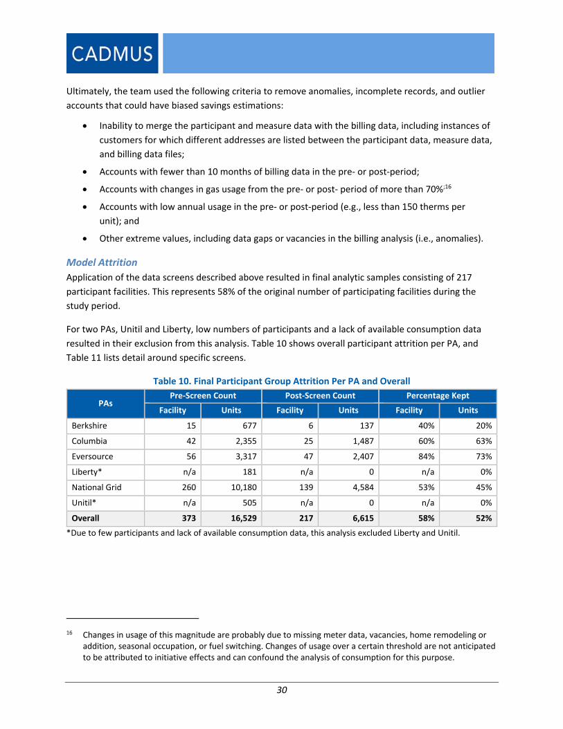
Application of the data screens described above resulted in final analytic samples consisting of 217 

participant facilities. This represents 58% of the original number of participating facilities during the 

study period. 

For two PAs, Unitil and Liberty, low numbers of participants and a lack of available consumption data 

resulted in their exclusion from this analysis. Table 10 shows overall participant attrition per PA, and 

Table 11 lists detail around specific screens. 

Table 10. Final Participant Group Attrition Per PA and Overall 

PAs Pre‐Screen Count Post‐Screen Count Percentage Kept

Facility  Units  Facility  Units  Facility  Units 

Berkshire  15  677 6 137 40%  20%

Columbia  42  2,355 25 1,487 60%  63%

Eversource  56  3,317 47 2,407 84%  73%

Liberty*  n/a  181 n/a 0 n/a  0%

National Grid  260  10,180 139 4,584 53%  45%

Unitil*  n/a  505 n/a 0 n/a  0%

Overall  373  16,529 217 6,615 58%  52%

*Due to few participants and lack of available consumption data, this analysis excluded Liberty and Unitil. 

 

                                                            

16   Changes in usage of this magnitude are probably due to missing meter data, vacancies, home remodeling or addition, seasonal occupation, or fuel switching. Changes of usage over a certain threshold are not anticipated to be attributed to initiative effects and can confound the analysis of consumption for this purpose. 

 

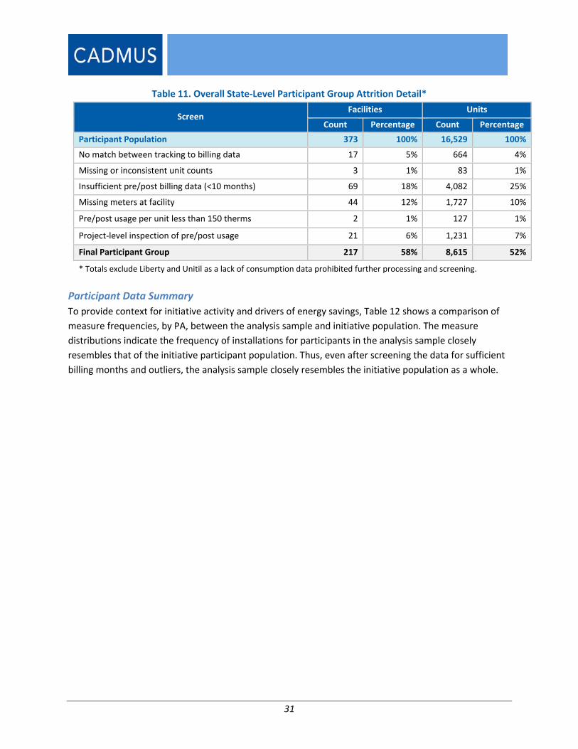
31 

Table 11. Overall State‐Level Participant Group Attrition Detail* 

Screen Facilities  Units 

Count  Percentage  Count  Percentage 

Participant Population  373 100%  16,529 100%

No match between tracking to billing data  17 5%  664 4%

Missing or inconsistent unit counts  3 1%  83 1%

Insufficient pre/post billing data (<10 months)  69 18%  4,082 25%

Missing meters at facility  44 12%  1,727 10%

Pre/post usage per unit less than 150 therms  2 1%  127 1%

Project‐level inspection of pre/post usage  21 6%  1,231 7%

Final Participant Group  217 58%  8,615 52%

* Totals exclude Liberty and Unitil as a lack of consumption data prohibited further processing and screening. 

 

Participant Data Summary  

To provide context for initiative activity and drivers of energy savings, Table 12 shows a comparison of 

measure frequencies, by PA, between the analysis sample and initiative population. The measure 

distributions indicate the frequency of installations for participants in the analysis sample closely 

resembles that of the initiative participant population. Thus, even after screening the data for sufficient 

billing months and outliers, the analysis sample closely resembles the initiative population as a whole.  

 

32 

Table 12. Comparison of Measure Distribution Between Sample and Population, per PA 

Category  Measure 

Berkshire  Columbia  Eversource National 

Grid 

Sample 

Population 

Sample 

Population 

Sample 

Population 

Sample 

Population 

Shell 

Air sealing  33% 64% 84% 80% 81%  75%  73% 72%

Insulation  33% 21% 72% 68% 79%  76%  58% 61%

Shell other  n/a n/a n/a n/a n/a  n/a  47% 48%

Windows  n/a n/a 4% 2% n/a  n/a  n/a n/a

HVAC 

Duct sealing and insulation  n/a n/a 32% 23% 19%  18%  7% 8%

Thermostats  n/a n/a n/a n/a 4%  2%  2% 3%

Heating system replacement  50% 43% 48% 41% 21%  25%  60% 55%

Water 

heating 

Aerators  n/a n/a 16% 16% n/a  n/a  57% 55%

Showerheads  n/a n/a n/a n/a n/a  n/a  47% 48%

DHW other  n/a n/a n/a n/a 32%  27%  39% 40%

Water heater replacement  n/a n/a 40% 30% n/a  n/a  63% 58%

Other**  Other  n/a n/a 8% 9% 11%  9%  40% 49%

Facility Count  6 14 25 44 47  55  139 260

* Variation in measure naming conventions across program tracking data resulted in differences in the level of detail measures were summarized by PA. ** This category includes custom projects, HVAC tune‐up/repair, and other miscellaneous measures (e.g., ventilation, moisture controls).  

 

Results This section presents evaluated gas savings estimates for the statewide and PA‐specific initiatives. 

Weather‐normalized annual consumption in the pre‐initiative period (PRENAC) is included in these 

results to characterize the average per unit energy consumption prior to any initiative treatment. 

Additionally, consideration of initiative impacts in terms of savings as a percentage of pre‐period usage 

(i.e., PRENAC) is a helpful metric for comparison purposes and for assessing the magnitude of initiative 

impacts, since this ratio normalizes these savings relative to consumption levels. 

 

33 

Model Results17 

Table 13 lists the changes in energy consumption from the pre‐ to post‐initiative periods for the 

participant group for each PA and at the statewide level.  

Table 13. LIMF Gross Natural Gas Participant Savings Per PA and Overall 

PA Group  Facilities (n)  Units (n)  PRENAC 

Model 

Savings 

(therm/unit) 

Savings as 

Percentage 

of Pre‐Usage 

Relative 

Precision at 

90% 

Berkshire  6  137 685 137 20%  ±41%

Columbia  25  1,487 561 107 19%  ±25%

Eversource  47  2,407 706 143 20%  ±17%

National Grid  139  4,584 581 124 21%  ±10%

Eversource + 

Columbia* 72  3,894 651 129 20%  ±15%

Overall**  217  8,615 607 126 21%  ±9%

* Given common approaches to delivery and estimating ex ante savings, the team combined Columbia and 

Eversource samples to increase sample size and provide modeled savings estimates with improved precision for 

calculating realization rates.  

**Overall state‐level results are population‐weighted, based on PA‐specific participant unit counts 

 Participants achieved estimated gross energy savings of 126 therms overall, while PA‐specific therm 

savings estimates vary slightly with percentage savings relative to pre‐period usage consistently 

between 19% and 21%.  

Table 14 lists realization rates for each PA and overall, based on the per‐unit evaluated savings 

compared to per‐unit ex ante savings. The table also shows savings percentages relative to PRENAC for 

both modeled and ex ante savings.  

                                                            

17   The Model Results section presents billing analysis results from the PRISM modeling approach, in which regressions are run on individual facilities. The team also ran combined fixed‐effects regression models for each group and found extremely comparable evaluated gross savings estimates. See Appendix D. 

 

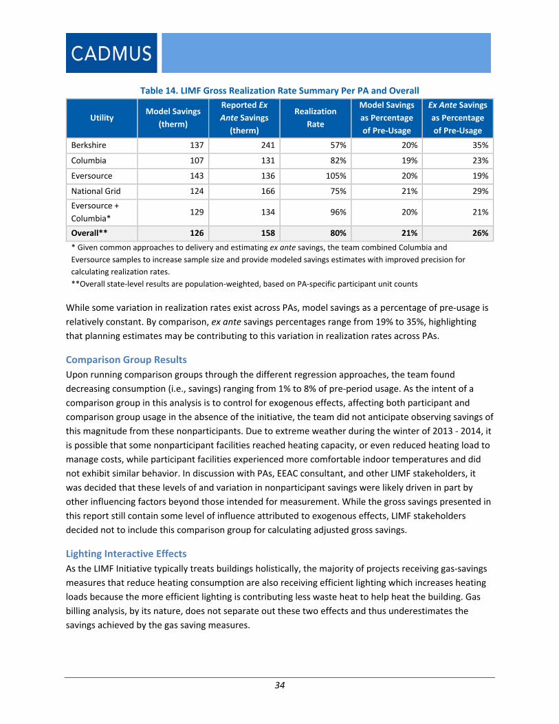
34 

Table 14. LIMF Gross Realization Rate Summary Per PA and Overall 

Utility Model Savings 

(therm) 

Reported Ex 

Ante Savings 

(therm) 

Realization 

Rate 

Model Savings 

as Percentage 

of Pre‐Usage 

Ex Ante Savings 

as Percentage 

of Pre‐Usage 

Berkshire  137  241 57% 20%  35%

Columbia  107  131 82% 19%  23%

Eversource  143  136 105% 20%  19%

National Grid  124  166 75% 21%  29%

Eversource + 

Columbia* 129  134 96% 20%  21%

Overall**  126  158 80% 21%  26%

* Given common approaches to delivery and estimating ex ante savings, the team combined Columbia and 

Eversource samples to increase sample size and provide modeled savings estimates with improved precision for 

calculating realization rates. 

**Overall state‐level results are population‐weighted, based on PA‐specific participant unit counts  

 While some variation in realization rates exist across PAs, model savings as a percentage of pre‐usage is 

relatively constant. By comparison, ex ante savings percentages range from 19% to 35%, highlighting 

that planning estimates may be contributing to this variation in realization rates across PAs.  

Comparison Group Results  

Upon running comparison groups through the different regression approaches, the team found 

decreasing consumption (i.e., savings) ranging from 1% to 8% of pre‐period usage. As the intent of a 

comparison group in this analysis is to control for exogenous effects, affecting both participant and 

comparison group usage in the absence of the initiative, the team did not anticipate observing savings of 

this magnitude from these nonparticipants. Due to extreme weather during the winter of 2013 ‐ 2014, it 

is possible that some nonparticipant facilities reached heating capacity, or even reduced heating load to 

manage costs, while participant facilities experienced more comfortable indoor temperatures and did 

not exhibit similar behavior. In discussion with PAs, EEAC consultant, and other LIMF stakeholders, it 

was decided that these levels of and variation in nonparticipant savings were likely driven in part by 

other influencing factors beyond those intended for measurement. While the gross savings presented in 

this report still contain some level of influence attributed to exogenous effects, LIMF stakeholders 

decided not to include this comparison group for calculating adjusted gross savings.  

Lighting Interactive Effects 

As the LIMF Initiative typically treats buildings holistically, the majority of projects receiving gas‐savings 

measures that reduce heating consumption are also receiving efficient lighting which increases heating 

loads because the more efficient lighting is contributing less waste heat to help heat the building. Gas 

billing analysis, by its nature, does not separate out these two effects and thus underestimates the 

savings achieved by the gas saving measures.  

 

35 

By assuming approximately one therm reduction for each efficient light replacing an incandescent bulb, 

this may result in approximately 1 to 15 therms per unit, depending on the average number of bulbs 

replaced per unit.18 While the modeled savings reflects the true change in consumption (i.e., the actual 

reduction in therms for the participant group), it may be appropriate to consider adjustments to the 

realization rates to back out the lighting interaction, treating this consistently across modeled and ex 

ante estimates. In this case, assuming replacement of five to 10 bulbs, the gross statewide realization 

rate of 80% would increase to somewhere between 83% and 89%.  

Model Diagnostics 

To provide context around the impact results, the team examined several different diagnostics and 

summaries of initiative data. The following figures present a comparison of modeled and ex ante savings 

as percentages of PRENAC, with Figure 2 showing differences per PA. It is apparent that realized savings 

are consistent across the PAs with ex ante values varying considerably. 

 Figure 3 shows a comparison of overall modeled and ex ante savings percentages by usage quartile. While percentage savings are comparable between ex ante and modeled savings in higher usage 

quartiles, Q1 and Q2 demonstrate substantially higher percentage ex ante savings. In fact, ex ante 

percentage savings in Q1 and Q2 are higher than those claimed on average for projects in higher usage 

quartiles. This seems to indicate planning estimates for lower usage quartiles may be overestimating the 

savings potential. 

Figure 4 shows a comparison of modeled and ex ante percentage savings by projects that received or did 

not receive heating system replacements. 

Figure 2. Model vs. Ex Ante Gross Savings as a Percentage of PRENAC Per PA 

  

                                                            

18   Cadmus, NMR. Impact Evaluation: Home Energy Services – Income Eligible and Home Energy Services Programs (R16). Presented to the Energy Conservation and Management Board, the Connecticut Light and Power Company, the United Illuminating Company, the Southern Connecticut Gas Company, Yankee Gas Services, and the Connecticut Natural Gas Company. 2014. Available Online: Final Report. 

 

36 

Figure 3. Model vs. Ex Ante Gross Savings as a Percentage of PRENAC Per Usage Quartile 

  

Figure 4. Model vs. Ex Ante Gross Savings as a Percentage of PRENAC  

  While projects without heating system replacements have lower average percentage savings, this is 

relatively consistent between modeled and ex ante estimates. Projects within heating system 

replacements demonstrate a larger difference between planning and evaluated results.  

Comparison of Realization Rate by Claimed Savings Type 

The evaluation team calculated ex ante savings estimates using two approaches: project‐specific 

simulation modeling and deemed calculated savings. For simulated savings, the team used actual usage 

to calibrate facility‐specific models, which then calculated a benefit/cost ratio to optimize measure 

installation for a given project. Table 15 provide a comparison of savings and realization rates for each 

type of claimed savings. 

While evaluated savings are similar in terms of absolute therm savings and percentage of PRENAC, the 

realization rate for projects claiming deemed ex ante savings show lower realization rates than for 

projects using simulation modeling. This is not surprising since simulation modeling should provide for a 

more accurate estimate of savings as it accounts for some level of measure interaction and is calibrated 

using actual usage data. 

 

37 

Table 15. LIMF Gross Natural Gas Participant Savings Per Claimed Savings Type 

Claimed Savings Type 

Facilities  PRENAC Model Savings (therms) 

Realization Rate 

Model Savings as Percentage of Pre‐Usage 

Ex Ante Savings as Percentage of Pre‐Usage 

Relative Precision at 90% 

Standard Algorithm 

139  581  124 75%  21% 29%  ±10%

Sim Modeled 

78  650  129 89%  20% 22%  ±14%

 

Benchmarking 

Benchmarking is always an important component of evaluation, to provide context around the results 

and how performance compares to other initiatives. The team was unable to identify many multifamily 

low‐income initiatives evaluated using billing analysis that delivered a similar mix of measures to 

benchmark against. Despite this limitation, the team compared these results against a range of recent 

evaluations of single family low‐income programs that evaluated whole‐building natural gas savings and 

whose programs deliver a similar combination of shell, water heating, and HVAC measures.19,20,21,22,23 

Figure 5 shows a comparison of the LIMF Initiative gross evaluated savings. 

Figure 5. Comparison of Evaluated Savings as a Percentage of PRENAC by Program 

  

                                                            

19   Cadmus, Low Income Single, 2012.  

20   Cadmus. Impact Evaluation: Rhode Island Income Eligible Services. Prepared for National Grid. 2014. 

21   Quantec, LLC. Ohio Home Weatherization Assistance Program Impact Evaluation. Prepared for Ohio Office of Energy Efficiency. 2006.  

22   Schweitzer, Martin. Estimating the National Effects of the U.S. Department of Energy’s Weatherization Assistance Program with State‐Level Data: A Metaevaluation Using Studies from 1993 to 2005. 2005.  

23   Cadmus, Impact Evaluation: Home Energy Services‐Income Eligible and Home Energy Services Programs. Prepared for the Connecticut Energy Conservation and Management Board. 2014. 

17%

21%

23%

16%

10%

22%

21%

0% 5% 10% 15% 20% 25%

 Midwestern Utility (Adj. Gross)

OH HWAP (Gross)

ORNL (meta)

RI IES (Gross)

CT HES‐IE (Gross)

MA LI (Adj. Gross)

MA LIMF ‐ Statewide (Gross)

Percentage Savings of PRENAC

 

38 

Figure 6 shows a comparison of the average per‐participant therm savings from the comparable studies. 

Absolute therm savings are lower for LIMF participants than the other comparable single‐family studies 

due to lower average pre‐period usage. As shown in Figure 5, in terms of savings percentage, the LIMF 

Initiative savings are consistent, if not higher, than other single‐family low‐income  

weatherization initiatives.  

Figure 6. Comparison of Evaluated Absolute Savings by Program 

  

180 

268 

305 

164

85 

249

126

0 50 100 150 200 250 300 350

 Midwestern Utility (Adj. Gross)

OH HWAP (Gross)

ORNL (meta)

RI IES (Gross)

CT HES‐IE (Gross)

MA LI (Adj. Gross)

MA LIMF ‐ Statewide (Gross)

Therm Savings

 

39 

Task 3. Common Area Lighting 

The review of tracking data for the electric LIMF Retrofit Initiative indicated that almost three‐quarters 

of electric LIMF Initiative savings resulted from lighting upgrades. Since the PAs had recently conducted 

research on in‐unit lighting measures and had not previously studied common area lighting in 

multifamily buildings, this task focused on lighting upgrades in common areas.  

Methods Common area lighting includes all lighting measures that occur outside an individual tenant unit. 

Therefore, this category included exterior lighting, parking garage lighting, and interior lighting in 

stairwells, hallways, common spaces, offices, and other non‐tenant spaces.  

For a sample of PY 2014 projects that included common area lighting measures, the team performed 

site visits to verify installed lighting equipment and install light loggers. The team used the collected data 

to estimate energy savings and compared the results to tracking data to determine realization rates of 

common area lighting measures implemented through the initiative.  

Sample Design 

The evaluation team reviewed the tracking documentation for lighting projects installed in PY 2014 and 

developed the evaluation sample. The team selected a sample by dividing the population into three 

strata based on the total common area lighting savings claimed for each project.  

Population 

Table 16 shows the number of tracked projects and annual savings (kWh) by PA for common area 

lighting projects implemented in PY 2014.  

Table 16. LIMF Lighting Projects and Savings by PA (PY 2014) 

PA Number of 

Projects 

% of Population

Projects Annual kWh Savings 

% of Population 

Savings 

National Grid  168  58% 5,342,356  33%

Eversource East  107  37% 9,462,307  59%

Eversource West  14  5% 1,307,665  8%

Unitil  1  0% 44,853  0%

Total  290  100% 16,157,180  100%

 Figure 7 shows the cumulative savings (across all PAs) based on the number of projects. The curve 

demonstrates a range in project sizes, with a small number of large projects that make up a majority of 

the savings, as well as a large number of small projects. 

 

40 

Figure 7. Cumulative Savings by Number of Projects 

 The evaluation team divided the population into three strata: 

Very Large Stratum. The very large stratum included all projects that were above the 95th 

percentile based on total energy savings (>179,193 kWh). This stratum, made up of 15 projects, 

accounted for 37% of the population annual energy savings. The team decided to pursue a 

census of these projects. By including as many of these projects in the evaluation sample as 

possible, the team eliminated sampling uncertainty for a large portion of the total savings, and, 

therefore, reduced sampling uncertainty in the overall estimate of total annual energy savings.  

Large stratum. The large stratum included the 130 projects with annual energy savings greater 

than the median value (21,791 kWh) that were not included in the very large stratum. These 

projects made up 53% of the population savings. 

Small stratum. The small stratum included the 145 projects with annual energy savings less than 

the median value (21,791 kWh). These projects made up 10% of the population savings. 

Table 17 summarizes how the team defined the three strata and shows each stratum’s share of the common area lighting population by number of projects and estimated annual kWh savings.  

Table 17. Definition of Common Area Lighting Population  

Strata Minimum 

Annual kWh Maximum Annual kWh 

Projects in Population  

Total Annual kWh Savings 

% of Population Savings 

Very Large  179,193  n/a 15 6,024,347  37%

Large Sample  21,792  179,192 130 8,554,016  53%

Small Sample  0  21,791 145 1,578,817  10%

Total  n/a  n/a 290 16,157,180  100%

 

 

41 

Sample 

Table 18 shows the sample of projects visited by strata and PA.  

Table 18. Number of Common Area Lighting Sample of Projects Visited and PA Per Strata 

Strata  Population  # Projects Visits PA 

National Grid Eversource

Very Large  15 10 1  9

Large  130 40 18  22

Small  145 6 2  4

Total  290 56 21  35

 The evaluation team attempted to visit all of the very large projects; however, due to site availability 

and scheduling constraints, the team was only able to visit 10 of the 15 projects. Table 19 shows the 

percentage of annual savings (kWh) within the population and the percentage of savings attributable to 

the projects we visited by each stratum.  

Table 19. Percentage of Annual kWh Savings by Population and Projects Visited Per Strata 

Strata % of Population 

(Annual kWh Savings)

% of Stratum Visited 

(Annual kWh Savings)

Very Large  37% 74% 

Large  53%   28%   

Small  10% 7% 

Total 100%  43% 

 The very large stratum makes up 37% of annual kWh savings from the entire population. The team 

visited 10 out of the 15 census sites, which account for 74% of the total savings from that stratum.  

Verification and Metering 

The evaluation team recruited customers through a two‐stage process. First, the team sent a 

recruitment letter to all applicable sites that explained the purpose of the evaluation and the activities 

that would take place on‐site; the letter also offered two $50 incentives to encourage participation. The 

letter gave recipients the option, if interested in participating, of contacting the evaluation team directly 

to arrange a visit. Second, the team called facility/building managers and explained the same material 

outlined in the letter. If the contact agreed to have the field technicians audit the site and install 

metering equipment, the team scheduled a visit. 

While on site, the evaluation team’s field technicians verified the installed lighting fixtures and 

compared their observations to the installed measures listed in the PA’s tracking data. They recorded 

number of fixtures installed, fixture type, location, and wattage whenever available. At each project, the 

technician also installed up to 10 meters to record the HOU of each fixture. As shown in Table 20, the 

field technicians installed two types of meters.  

 

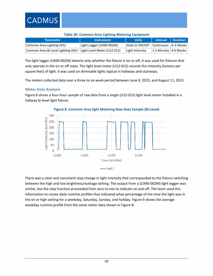
42 

Table 20. Common Area Lighting Metering Equipment 

Parameter  Instrument Units Interval  Duration

Common Area Lighting HOU  Light Logger (UX90‐002M) State or ON/OFF  Continuous  4–6 Weeks

Common Area Bi‐Level Lighting HOU  Light Level Meter (U12‐012) Light Intensity 1.5 Minutes  4‐6 Weeks

 The light logger (UX90‐002M) detects only whether the fixture is on or off; it was used for fixtures that 

only operate in the on or off state. The light level meter (U12‐012) records the intensity (lumens per 

square feet) of light; it was used on dimmable lights typical in hallways and stairways.  

The meters collected data over a three to six week period between June 9, 2015, and August 11, 2015.  

Meter Data Analysis 

Figure 8 shows a four‐hour sample of raw data from a single (U12‐012) light level meter installed in a 

hallway bi‐level light fixture.  

Figure 8. Common Area light Metering Raw Data Sample (Bi‐Level) 

  There was a clear and consistent step change in light intensity that corresponded to the fixture switching 

between the high and low brightness/wattage setting. The output from a (UX90‐002M) light logger was 

similar, but the step function proceeded from zero to one to indicate on and off. The team used this 

information to create daily runtime profiles that indicated what percentage of the time the light was in 

the on or high setting for a weekday, Saturday, Sunday, and holiday. Figure 9 shows the average 

weekday runtime profile from the same meter data shown in Figure 8.  

 

43 

Figure 9. Sample Weekday Common Area Light Runtime Profile (Bi‐Level) 

 Since the bi‐level lighting was occupancy controlled, it was not surprising that the light was at the high 

setting most frequently from 12:00 p.m. to 9:00 p.m. and on the low setting most frequently from  

12:00 a.m. to 8:00 a.m.  

Figure 10 and Figure 11 show the distribution of the metered HOU for the bi‐level hallway and stair 

space types. 

Figure 10. Stairway HOU Distribution High Level (Bi‐Level) 

  

 

44 

Figure 11. Hallway HOU Distribution at High Level (Bi‐Level) 

  Interior common area lighting in LIMF buildings typically operate 24 hours per day, seven days per week 

or are controlled by a timer/occupancy sensor. As such, it is likely that the interior lighting had negligible 

seasonal dependence. The evaluation team estimated annual hours of use by extrapolating the 

computed daily runtime profiles over the entire year.  

The team confirmed that exterior lighting operated through a timer or occupancy control. The current 

estimate of 12 hours per day for exterior was reasonable when compared to secondary research, which 

confirmed average daily hours of darkness for Massachusetts as 11 hours and 47 minutes.24 Where 

exterior metering did occur, the team normalized data for photocell‐controlled lighting using the hours  

of darkness.  

Action and ABCD both acknowledged that bi‐level exterior lighting is generally not cost‐effective, but 

both are open to looking for opportunities to implement this measure. 

Sample Analysis 

The evaluation team calculated the realization rate for each stratum using the following equation:  

∑ ∑

 

The team then extrapolated the realization rate for each stratum to the stratum population and 

summed the stratum population ex post savings to estimate ex post savings for the total LIMF total 

population of common area lighting projects. 

                                                            

24   U.S. Naval Observatory. Duration of Daylight/Darkness Table for One Year. 2015. Available online: http://aa.usno.navy.mil/data/docs/Dur_OneYear.php. 

 

45 

Results Table 21 lists the realization rate and relative precision for National Grid, Eversource, and statewide. 

These results are based on installed fixture verification and time‐of‐use metering for 56 common area 

lighting projects in the PY 2014 LIMF Initiative.  

Table 21. Common Area Metering Equipment 

PA  Realization Rate Relative Precision 

at 90% Confidence 

National Grid  101% ±8%

Eversource  96% ±2%

Statewide  97% ±3%

 All realization rates are close to 100% indicating the actual energy savings are similar to the ex ante estimates from the implementation contractors. 

Deemed Savings Value 

Given the highly varied nature of common area lighting, the team suggests estimating savings using an 

algorithm that incorporates site‐specific information whenever possible. However, Table 22 provides 

deemed savings values for PAs that do not calculate savings using site‐specific inputs.  

Table 22. Common Area Lighting Deemed Savings Values 

Space Type Qty New 

Fixtures 

Ex Ante Savings 

(kWh/yr) 

Per Fixture Ex 

Ante Savings 

(kWh/yr) 

Realization 

Rate 

Per Fixture Ex Post 

Savings (kWh/yr) 

Exterior  11,639 6,851,891 589 97% 571

Interior  32,225 9,305,289 289 97% 280

 The team separated interior and exterior lighting because exterior lighting tends to use higher wattage fixtures and consistently operates for 4,380 hours per year resulting in significantly higher savings than interior fixtures. The team calculated a deemed value using the quantity of interior and exterior fixtures installed, the ex ante savings, and the statewide realization rate.  

Findings Related to Pre‐Installation Fixture Wattage 

For one National Grid project, the team found a discrepancy between the tracking data and on‐site 

observations regarding the pre‐installation fixture information. For this project, the tracking data listed 

the pre‐fixture wattage as 190 watts. During the on‐site verification activities, the team found an 

existing pre‐installation fixture (which had been repurposed) with a nameplate of a 70‐watt high 

pressure sodium lamp. The facility contact confirmed the 70‐watt lamp represented pre‐installation 

fixtures for the project. For this observed fixture, the actual pre‐installation fixture wattage would be 95 

watts including the ballast, much lower than the 190‐watts‐per‐fixture estimate in the tracking data.  

 

46 

Due to the large quantity of these fixtures in the project, this discrepancy in the pre‐installation fixture 

wattage could have a large impact on the evaluated results for the project. Including the pre‐installation 

fixture adjustment in the evaluated savings calculation resulted in a realization rate of 55% for the site.  

Without the pre‐installation fixture adjustment the adjustment, the project realization rate is 102% (due 

to higher metered hours of use).  

Through stakeholder discussions about these evaluation findings, the team determined not to include 

the pre‐installation adjustment in the final results.  The evaluation results only include adjustments to 

post‐installation fixture counts and wattage and to annual hours of use estimates (based on metered 

data). To minimize potential for future errors in the documentation of pre‐installation fixture wattage 

and to support future evaluation efforts, the PAs should, if they have not already, develop protocols for 

collecting and verifying pre‐installation wattages that include taking photographs of each type of 

replaced fixture.  

 

47 

Task 4. On‐Site Verification and Measure Analysis  

While installing light meters on‐site for Task 3, the evaluation team investigated several specific 

measures identified as of particular interest during the stakeholder workshops. This activity provided 

third‐party verification of measure installations and allowed for additional data collection at the 

customer facility. The field technicians set out to investigate the following measures: 

Showerheads and aerators 

Condensing boilers 

Water heating systems 

Air conditioning (AC) units  

Energy management systems (EMS)/controls  

Variable frequency drives (VFD)  

The team completed the following for this task:  

1. Examined the persistence of measures at risk of removal (e.g., showerheads and aerators);  

2. Collected detailed system information to supplement the billing analysis;  

3. Discussed building operation and performance with facility managers to collect anecdotal 

feedback.  

The field technicians did not encounter any instances of EMS/controls or VFDs at the sample of projects 

they visited. The remaining measures were assessed. 

Showerheads and Aerators Showerheads and faucet aerators reduce water consumption and water heating fuel (electrical energy 

or natural gas consumption). However, users do not always embrace these devices, so there is the risk 

that over time, they may be removed or replaced with less efficient models.  

Methods 

At each project where the team determined faucet aerators or showerheads had been installed, field 

technicians asked the building manager to let them into five units to inspect the installed equipment. 

The field technicians provided $10 incentives to each resident that allowed them into their homes. 

When inside, the technicians recorded the rated flow rate of all faucet aerators and showerheads within 

the unit. Typically, the field technicians observed one kitchen faucet aerator, one bathroom faucet 

aerator, and one showerhead.  

Results 

In the sample, the evaluation team found five projects with faucet aerators and/or showerheads 

installed as part of the initiative. For one of these projects, the building manager declined to allow the 

 

48 

field technicians into the tenant units. At each of the four remaining projects, the field technicians 

entered five units.  

Among the projects that the technicians inspected, the implementers always installed kitchen faucet 

aerators, but bathroom faucet aerators and showerheads were installed only in some of the units. Table 

23 lists which measures were installed in the project units the field technicians inspected.  

Table 23. Faucet Aerator and Showerhead Installations Per Project Site 

Project # Kitchen Faucet Aerators Bathroom Faucet Aerators Showerheads 

1   

2   

3   

4   

 To calculate savings for faucet aerators and showerheads, the TRM suggests using deemed values. The 

TRM specifies the flow rate of faucet aerators should not exceed 1.5 gallons per minute (GPM) and 

showerheads should not exceed 2.5 GPM. Figure 12 shows the distribution of flow rates observed 

among the units inspected.  

Figure 12. Distribution of Observed Faucet Aerators and Showerheads by Rated Flow Rate 

  To calculate the in‐service rate (ISR) of each measure, the evaluation team divided the number of 

observed faucet aerators and showerheads that were below the maximum allowable flow rate threshold 

and divided by the total number found during the project audit. Table 24 shows the quantity of faucet 

aerators and showerheads observed below the allowable threshold, total inspected, and computed ISR.  

 

49 

Table 24. ISR Calculation for Faucet Aerators and Showerheads 

Parameter  Value 

Faucet Aerators

Quantity Below 1.5 GPL 27

Total Faucets 34

Faucet ISR 79%

Showerheads

Quantity Below 2.5 GPL 10

Total Showerheads 10

Showerhead ISR 100%

 Due to the low number of these measures observed, the team does not recommend adopting these ISR 

values. However, the data suggest faucet aerators do not persist; therefore, the total achievable savings 

are often not realized. A more extensive study is required to obtain statistically significant results. 

However, since these measures account for a small percentage of total LIMF Initiative savings, the 

expense of such a study may outweigh its benefit.25   

Air Conditioning Equipment The purpose of this task was to determine what, if any, air conditioning systems LIMF buildings use and 

quantify the prevalence of room air conditioners (RAC) and central air conditioning systems (CAC). 

Methods 

At each of the 56 projects the field technicians visited, they discussed the air conditioning systems with 

site personnel. If the building used CACs, they inspected the units and recorded nameplate information. 

If the building used RACs, they determined whether they were supplied by the building or owned by the 

tenant. 

Results 

The evaluation team divided the air conditioning systems observed at the projects sites into eight 

categories. Table 25 lists the defined categories and shows the prevalence of each system in terms of 

quantity observed and percentage of the total.  

                                                            

25   Aerators and showerheads accounted for 0.2% of LIMF kWh savings and 2.1% of LIMF therm savings in  PY 2013. (Cadmus, MA LIMF Technical, 2014) 

 

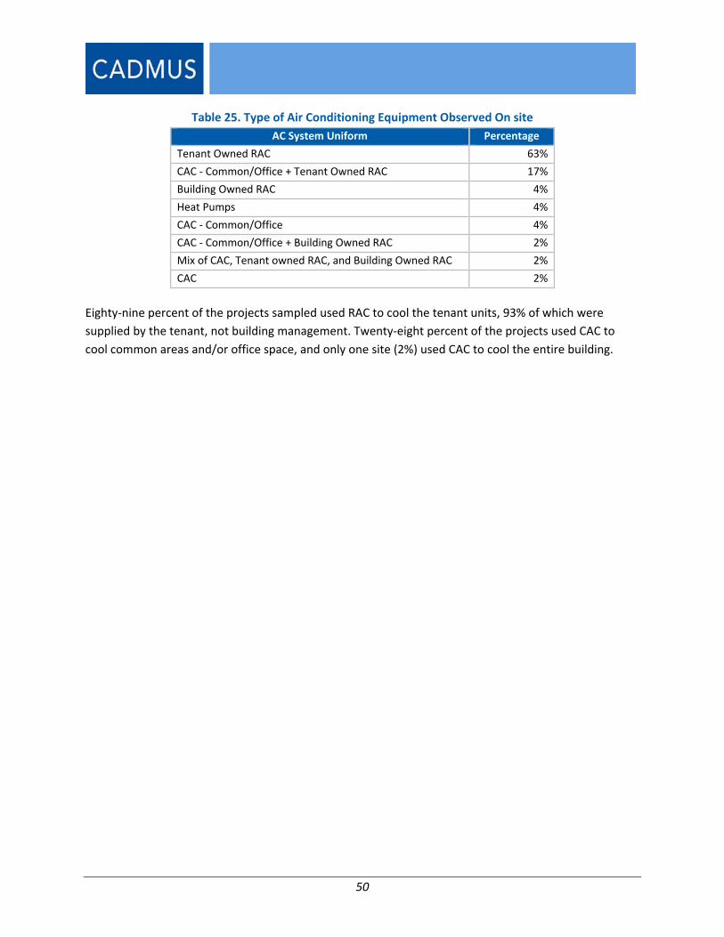
50 

Table 25. Type of Air Conditioning Equipment Observed On site 

AC System Uniform Percentage 

Tenant Owned RAC  63% 

CAC ‐ Common/Office + Tenant Owned RAC 17% 

Building Owned RAC  4% 

Heat Pumps  4% 

CAC ‐ Common/Office  4% 

CAC ‐ Common/Office + Building Owned RAC 2% 

Mix of CAC, Tenant owned RAC, and Building Owned RAC 2% 

CAC  2% 

 Eighty‐nine percent of the projects sampled used RAC to cool the tenant units, 93% of which were 

supplied by the tenant, not building management. Twenty‐eight percent of the projects used CAC to 

cool common areas and/or office space, and only one site (2%) used CAC to cool the entire building.  

 

51 

Task 5. Assessment of Secondary Impacts 

Several measures installed as part of the LIMF Initiative result in secondary benefits. During the 

technical review phase, the evaluation team found that the PAs did not uniformly claim savings for all of 

these measures. The purpose of this task was to improve consistency in measuring and estimating 

savings among the PAs by clearly outlining acceptable secondary savings.  

The team focused on two areas: water savings and cooling energy savings resulting from weatherization. 

Similar to Task 1, the team evaluated the approaches for calculating these savings outlined in the TRM 

and determined a recommended approach. 

Water Savings Three measures currently implemented as part of the LIMF Initiative result in water savings: faucet 

aerators, showerheads, and clothes washers. The evaluation team recommends the PAs track savings 

for each of these measures since water savings is a quantifiable benefit.  

Methods 

Similar to the methods employed in Task 1. Engineering Analysis and Literature Review, the team 

reviewed the savings calculations outlined in the TRM, the cited sources, and other secondary resources 

(e.g., ENERGY STAR calculator) to determine the best approach to calculating savings. 

Faucet Aerator Savings 

To estimate water savings from faucet aerators, the team used the following equation:  

∆ 365 

Where: 

∆   =  Annual water savings (gallons/year) 

  =  Baseline flow rate (gallons/minute) 

  =  Installed flow rate (gallons/minute) 

  =  Average number of people per household

  =  Daily minutes of water use per person 

365  =  Days per year 

 The evaluation team calculated the water savings from kitchen and bathroom faucet aerators 

individually and then computed a weighted average based on the number of kitchen aerators and 

bathroom aerators typically installed in a unit.  

Table 26 lists the input assumes used to estimate annual water savings from low‐flow bathroom and 

kitchen aerators.  

 

52 

Table 26. Faucet Aerator Water Saving Calculation Inputs 

Input 

Values 

Units  Source Bathroom Aerator 

KitchenAerator 

Low‐Flow Equipment 

Baseline flow rate ‐ rated  1.30  1.30 gallons/min  Federal standard 

Installed flow rate ‐ rated  1.00  1.00 gallons/min  Average installed (for this study) 

Reduction in flow rate  0.30  0.30 gallons/min  (calculated) 

Water Consumption 

Household members  2.30  2.30 people Low‐income audit data 

(Cadmus, Low Income, 2012)* 

Daily use per person  1.65  4.51 minutes/person/day Cadmus, Showerhead and 

Faucet, 2013* 

Minutes of use per day  3.8  10.4 minutes/day  (calculated) 

Water Savings 

Water savings per day  1.14  3.105 gallons/day  (calculated) 

Water savings per year  416  1,133 gallons/year  (calculated) 

* See Appendix C for full citations. 

 Table 27 shows assumptions used to estimate the weighted average water savings for bathroom and 

kitchen aerators.  

Table 27. Average Faucet Aerator Water Saving 

Input  Values  Units Source 

Average kitchen aerators installed  1.03  aerators/apartment  Cadmus, Home Energy, 2012* 

Average bathroom aerators installed  1.50  aerators/apartment  Cadmus, Home Energy, 2012* 

Weighted average water savings  708  gallons/year/aerator  (calculated) 

* See Appendix C for full citations. 

 The Massachusetts TRM currently assigns water savings of 332 gallons per year, but does not distinguish 

between kitchen and bathroom aerators.26 The inputs listed in Table 26 and Table 27 are more relevant 

to the Massachusetts LIMF Initiative.  

Showerhead Savings 

The team estimated water savings from showerheads using the following equation:  

                                                            

26   KEMA. Evaluation of the Weatherization Residential Assistance Partnership (WRAP) and Helps Programs. 2010. Presented to the Energy Conservation and Management Board, the Connecticut Light and Power Company, the United Illuminating Company, the Southern Connecticut Gas Company, Yankee Gas Services, and the Connecticut Natural Gas Company. 

 

53 

∆ % 365 

Where: 

∆   =  Annual water savings (gallons/year) 

  =  Baseline flow rate (gallons/minute) 

  =  Installed flow rate (gallons/minute) 

  =  Average number of people per household 

  =  Showers per person per day 

  =  Shower length 

%Impact  =  Proportion of showering activity affected by replacement 

365  =  Days per year 

 The evaluation team set the as‐used water flow rate equal to the maximum rated flow after scaling it 

back linearly to account for water pressure at the residence that is less than 80 psi rating pressure. Table 

28 shows the values and sources of all the inputs the team used to estimate showerhead savings.  

Table 28. Showerhead Savings Calculation Inputs 

Input  Values  Units  Source 

Low‐Flow Equipment 

Baseline flow rate ‐ rated  2.50 gallons/min  Federal standard 

Baseline flow rate ‐ as used  2.05 gallons/min  Calculated (Cook, 2008)* 

Installed flow rate ‐ rated  2.00 gallons/min  Average Installed [this study] 

Installed flow rate ‐ as used  1.78 gallons/min  Calculated (Cook, 2008)* 

Reduction in flow rate  0.50 gallons/min  (calculated) 

Water Consumption 

Household Members  2.30 people Low‐income audit data (Cadmus, 

Low Income, 2012)* 

Showers (pcpd)  0.70 showers/person/day (Cadmus, Low Income, 2012), (Cook, 

2008), (Mayer, 2006)* 

Shower Length (min)  8.20 minutes/shower (Cadmus, Low Income, 2012), 

(Biermayer, 2006), (Mayer, 2006)* 

Proportion Affected  0.73 %  HES audit data 

Minutes of use per day  9.6 minutes/day  (calculated) 

Water Savings 

Water savings per day  4.82 gallons/day  (calculated) 

Water savings per year  1,759 gallons/year  (calculated) 

* See Appendix C for full citations. 

 The value currently proposed in the TRM (3,696 gallons per year) is higher than the value calculated in 

Table 28. The team calculated this value using the rated flow as opposed to the as‐used flow rate and 

 

54 

assumed an average shower lasts 12.2 minutes instead of 8.2 minutes. In the report providing the value 

in the TRM, they explain, “[we] suspect that the reported usage of 12.2 minutes per shower per day may 

be overstated, because of a tendency of respondents to overstate the frequency with which they 

actually take showers, but there are no data on this specific population to refute this claim.”(KEMA, 

2010). Based on additional secondary data sources, the team considers 8.2 minutes per shower a more 

accurate value.27 

Clothes Washer Savings 

The team estimated savings for clothes washers using the ENERGY STAR calculator. For clothes washers 

installed in shared laundry rooms in multifamily residences, the calculator assumes a capacity of 2.8 

cubic feet, a modified energy factor of 2.2, a water factor of 4.5, and that the machine washes 24 loads 

per week. Using these inputs, the calculator estimated each washer will save 6,948 gallons per year. This 

value is smaller than the value in the 2014 TRM (15,813 gallons per year) which is based on an outdated 

baseline.  

Interactive Cooling Impacts The implementation of measures such as insulation and air sealing improves a home’s building envelope 

and typically results in reduced heating and cooling loads. The purpose of this activity was to quantify 

the cooling energy savings attributable to weatherization measures. 

Methods 

Based on data collected from on‐site visits, the team determined that RAC units comprised the majority 

of AC equipment installed at LIMF sites. The team estimated savings due to weatherization 

improvements for RAC units using the following equations: 

/

11000

 

∆ % %  

Results 

Table 29 shows the inputs the evaluation team used to calculate cooling savings due to weatherization. 

                                                            

27   Cadmus, Low Income, 2012; Biermayer 2006; and Mayer 2006. See Appendix D for full citations.  

 

55 

Table 29. Inputs to Calculate Weatherization Cooling Savings of RAC Units  

Parameter  Definition  Value  Source 

EFLHCool  Equivalent full load hours (cooling)  200 RLW Analytics, 2008* 

RAC BTU/hr  Capacity  10,000 ENERGY STAR calculator 

RAC EER  Baseline energy efficiency ratio  6.7

Laboratory testing of older, but 

operable window air 

conditioners (Cadmus, OPA 

Keep, 2008)* 

% Cooling from 

Weatherization 

Percentage of home cooling load impacted by 

weatherization characteristics 40% Cadmus, New Hampshire, 2013* 

% Savings Percentage of reduction in cooling energy 

due to installed weatherization measures 18.3% Cadmus, New Hampshire, 2013* 

Savings per Unit  Annual kWh savings per RAC unit  22 Calculated 

* See Appendix C for full citations. 

 Table 30 compares estimated from air sealing and insulation during the heating and cooling seasons. 

The team calculated these savings using the Deemed Savings Workbook (Tasl 1) for a typical multifamily 

unit.  

Table 30. Typical Weatherization Savings 

Measure  Annual Savings (kWh) 

Air Sealing (Heating)  397

Insulation (Heating)  1,377

Weatherization (Cooling) 22

 Based on the values in Table 30, savings during the cooling season account for only 1.2% of the total 

energy savings from weatherization. Since many of the tenants are responsible for installing the RACs in 

the LIMF buildings (93% according to the data collected on site), some building units do not contain any 

AC equipment. Thus, on a building or initiative level, the actual savings per tenant unit will be less than 

estimated above. Since it is would require additional effort to track, the evaluation team does not 

recommend adding energy savings due to weatherization upgrades from the cooling period.  

 

 

 

56 

Appendix A. Summary of Deemed Savings Values 

Figure 13. Deemed Savings Summary ‐ Electric 

 

Deemed Savings Summary for LIMF Program (Electric)

Program year: 2016

kWh** therms water 2014 2013 NGRID Eversource CLC Unitil

1 Misc TLC Kit User Input 70 n/a 432 [1] n/a n/a unk unk unk unk

1a Misc TLC Kit (Eversource 0941) Deemed 69 n/a n/a [1] 18 18 unk 25 unk unk

1b Misc TLC Kit (Eversource 0971) Deemed 69 n/a n/a [1] 18 18 unk 25 unnk unk

1c Misc TLC Kit (CLC) Deemed 152 n/a 863 [1] 126 128 unk unk 126 unk

2 Lighting Torchiere (2016)* Deemed 55.1 n/a n/a [2] 211 211 unk 211 unk unk

3 Lighting CFL Bulb (2016)* Deemed 40.8 n/a n/a [2] 47.9 48.5 unk 41 48.5 41

4 Lighting LED Bulb (2016)* Deemed 55.1 n/a n/a [2] 51.5 54.7 unk 41 54.7 54.7

5 Lighting Common Area Fixture (Exterior) Deemed 571 n/a n/a [10] 100.5 100.5 unk unk unk unk

6 Lighting Common Area Fixture (Interior) Deemed 280 n/a n/a [10] 140 140 unk unk unk unk

7 Wx Air Sealing, Electric User Input 338 n/a n/a [9] n/a n/a unk unk unk 309

8 Wx Insulation, Electric User Input 1,377 n/a n/a [9] n/a n/a unk unk unk unk

9 HVAC Heating System Retrofit Deemed 133 n/a n/a *** 132 133 unk unk unk unk

10 HVAC Thermostat, Electric Deemed 257 n/a n/a *** 257 257 unk 257 unk 257

11 HVAC Demand Circulator, Electric User Input 560 n/a n/a [11] n/a n/a unk 5,320 unk 5,320

12 HVAC Pipe Wrap, Electric Deemed 129 n/a n/a *** 129 129 unk unk 129 unk

13 DHW Heat Pump Water Heaters (50 Gallon) Deemed 1,687 n/a n/a [3] 1,775 1,775 unk 1,775 unk unk

14 DHW DHW Tank Wrap, Electric Deemed 73 n/a n/a [4] 73 73 55 134 unk unk

15 DHW Showerhead, Electric Deemed 217 n/a 1,759 [5] 129 129 129 unk unk 129

16 DHW Faucet Aerator (All), Electric Deemed 62 n/a 708 [5] 97 97 97 unk unk 97

17 DHW Faucet Aerator (Kitchen), Electric Deemed 106 n/a 1,133 [5] 97 97 97 unk unk 97

18 DHW Faucet Aerator (Bathroom), Electric Deemed 31 n/a 416 [5] 97 97 97 unk unk 97

19 Appliances Window AC Replacement Deemed 113 n/a n/a [6] 204 204 unk 204 unk 204

20 Appliances Refrigerator Deemed 330 n/a n/a [7] 645 645 unk 645 762 unk

21 Appliances 2nd Refrigerator Removal Deemed 874 n/a n/a [7] 1,180 1,180 unk 645 1,180 unk

22 Appliances Freezer Replacement Deemed 158 n/a n/a [7] 239 239 unk 637 unk 637

23 Appliances Clothes Washer Deemed 318 13 6,948 [8] 1,218 1,218 unk unk unk 1,218

24 Appliances Smart Strip Deemed 79 n/a n/a *** 79 79 79 79 79 79

25 Appliances Waterbed Deemed 872 n/a n/a *** 872 872 unk 872 unk unk

NOTES:

* 

*** Proposed deemed savings values are the same or similar to the values used in 2013. 

Existing Values for ComparisonProposed Values for PY2016+

MA TRM (kWh/year) 2013 Savings Estimates by PA (kWh/year)# NOTESTypeMeasureEnd‐Use

Annual Savings Value

Indicates that deemed savings value is dependent on the selected program year

 

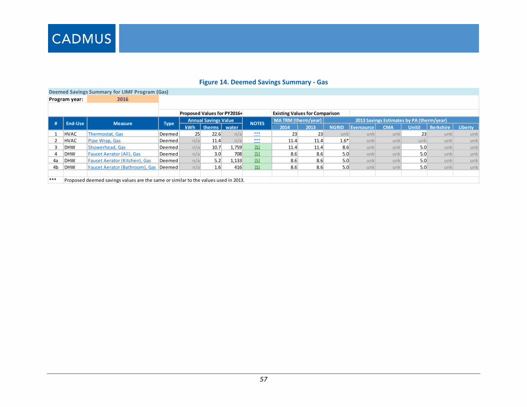
57 

 

Figure 14. Deemed Savings Summary ‐ Gas 

 

 

 

Deemed Savings Summary for LIMF Program (Gas)

Program year: 2016

Existing Values for Comparison

kWh therms water 2014 2013 NGRID Eversource CMA Unitil Berkshire Liberty

1 HVAC Thermostat, Gas Deemed 25 22.6 n/a *** 23 23 unk unk unk 23 unk unk

2 HVAC Pipe Wrap, Gas Deemed n/a 11.4 n/a *** 11.4 11.4 1.6* unk unk unk unk unk

3 DHW Showerhead, Gas Deemed n/a 10.7 1,759 [5] 11.4 11.4 8.6 unk unk 5.0 unk unk

4 DHW Faucet Aerator (All), Gas Deemed n/a 3.0 708 [5] 8.6 8.6 5.0 unk unk 5.0 unk unk

4a DHW Faucet Aerator (Kitchen), Gas Deemed n/a 5.2 1,133 [5] 8.6 8.6 5.0 unk unk 5.0 unk unk

4b DHW Faucet Aerator (Bathroom), Gas Deemed n/a 1.6 416 [5] 8.6 8.6 5.0 unk unk 5.0 unk unk

***

#

Proposed deemed savings values are the same or similar to the values used in 2013. 

2013 Savings Estimates by PA (therm/year)

Proposed Values for PY2016+

MA TRM (therm/year)End‐Use Measure Type NOTES

Annual Savings Value

 

58 

Appendix B. Billing Analysis Model Specification 

PRISM Model The evaluation team used the heating PRISM model to estimate savings in both the pre‐ and post‐period 

for each customer (i.e., facility) using the following specification: 

 

Where, for each facility “i”, calendar month “t”, and HDD base: 

ADCit   =  average daily therm consumption in the pre‐ or post‐initiative period. 

i   =  the participant intercept, representing the average daily therm base load.  

β1   =  the model space heating slope. 

AVGHDDit   =  the variable base 50 to 65 average daily HDDs for the specific location. 

it   =  the error term. 

Using the above models, the team calculated weather‐NAC using the following equation: 

∗ 365  

Where, for each facility “i”: 

NACi     =  normalized annual therm consumption. 

I    =  the intercept equaling the average daily or base load for each participant,  

      representing the average daily base load from the model. 

i * 365    =  annual base‐load therm usage (non‐weather sensitive). 

β1     =  the heating slope (in effect, usage per heating degree from the model above). 

LRHDDi    =  the annual, long‐term HDDs (base 50 to 65) of a TMY3 in the 1991–2005 series 

  from NOAA, based on home location 

β1 * LRHDDi =  weather‐normalized, annual weather‐sensitive (heating) usage 

(i.e., HEATNAC) 

I     =  the error term 

After running through all models across variable HDD base temperatures, the best model for each facility “i” is the model with highest R‐squared. 

Combined Fixed‐Effects Model To estimate gas energy savings, the team used a pre‐ and post‐installation savings analysis fixed‐effects 

modeling method, which used pooled monthly time‐series (panel) billing data. The fixed‐effects 

modeling approach corrected for the following:  

1. Differences between pre‐ and post‐installation weather conditions; and  

 

59 

2. Differences in usage consumption between participants, through inclusion of a separate 

intercept for each participant.  

This modeling approach ensured that model savings estimates would not be skewed by unusually high‐

usage or low‐usage participants. The following model specification determined overall savings: 

∗  

Where for each facility “i” and monthly billing period “t”: 

ADC it     =  the average daily therm consumption during the pre‐ or post‐installation initiative period. 

i    =  the average daily therm base‐load intercept for each customer. (This is      part of the fixed‐effects specification.) 

    =  the baseline usage per HDD for each customer. 

AVGHDDit    =  the average daily PRISM base HDDs, based on home location. 

β1    =  the average daily whole‐house base‐load therm savings.  

POSTi    =  an indicator variable that is 1 in the post‐period (after the latest    measure installation) and 0 in the pre‐period (prior to participation). 

β2    =  the whole‐house heating therm savings per heating degree‐day. 

POSTi * AVGHDDit  =  an interaction between the POST indicator variable and the average   daily PRISM base heating degree‐days (AVGHDD). 

it    =  the modeling estimation error. 

 

 

 

60 

Appendix C. References 

Biermayer, Peter J. Potential Water and Energy Savings from Showerheads. Prepared for the Lawrence 

Berkeley National Laboratory. 2006. 

Cadmus. OPA Keep Cool Metering Study. Prepared for the Ontario Power Authority. 2008. 

Cadmus. Home Energy Services Impact Evaluation. Prepared for Massachusetts Program Administrators. 

2012. 

Cadmus. Low Income Single Family Program Impact Evaluation. Prepared for the Electric and Gas 

Program Administrators of Massachusetts. 2012. Available online at: http://ma‐eeac.org/wordpress/wp‐

content/uploads/Low‐Income‐Single‐Family‐Program‐Impact‐Evaluation_Part‐of‐the‐Massachusetts‐

Residential‐Retrofit‐Low‐Income‐Program‐Area‐Evaluation.pdf  

Cadmus. New Hampshire HVAC Load and Savings Research: Final Report. Prepared for New Hampshire 

Public Utilities Commission and the New Hampshire Monitoring and Evaluation Team. 2013. 

Cadmus and Opinion Dynamics. Showerhead and Faucet Aerator Meter Study. Prepared for Michigan 

Evaluation Working Group, 2013.  

Cadmus. Impact Evaluation: Rhode Island Income Eligible Services. Prepared for National Grid. 2014. 

Cadmus, NMR. Impact Evaluation: Home Energy Services – Income Eligible and Home Energy Services 

Programs (R16). Presented to the Energy Conservation and Management Board, the Connecticut Light 

and Power Company, the United Illuminating Company, the Southern Connecticut Gas Company, Yankee 

Gas Services, and the Connecticut Natural Gas Company. 2014. Available Online: 

http://www.energizect.com/government‐municipalities/hes‐and‐hes‐ie‐impact‐evaluation‐r16‐final‐

report‐12‐31‐14 

Cadmus. MA LIMF Technical Review Summary of Findings Memo. Prepared for the Electric and Gas 

Program Administrators of Massachusetts. 2014. 

Cook, G. and B. Barkett. Resource Savings Values in Selected Residential DSM Prescriptive Program. 

Prepared for Summit Blue Canada Inc. 2008. 

Internal Performance Measurement & Verification (IPMVP) Committee. Concepts and Options for 

Determining Energy and Water Savings: Volume 1. IPMVP Option C. 2002. Available online: 

http://www.nrel.gov/docs/fy02osti/31505.pdf 

KEMA. Evaluation of the Weatherization Residential Assistance Partnership (WRAP) and Helps Programs. 

Presented to the Energy Conservation and Management Board, the Connecticut Light and Power 

Company, the United Illuminating Company, the Southern Connecticut Gas Company, Yankee Gas 

Services, and the Connecticut Natural Gas Company. 2010. 

 

61 

Massachusetts Energy Efficiency Advisory Council. Annual Results Tables: 2014 Electric and Gas 

Statewide Summaries. Available online: http://ma‐eeac.org/results‐reporting 

Mayer, P.W., et al. Residential End Uses of Water. Prepared for AWWA Research Foundation. 1999. 

(Referenced by Biermayer 2006.) 

National Renewable Energy Laboratory. UMP Whole‐Building Retrofit with Consumption Data Analysis 

Evaluation Protocol. 2013. Available online: https://www1.eere.energy.gov/wip/pdfs/53827‐8.pdf. 

Opinion Dynamics Corporation. Massachusetts Residential Appliance Saturation Survey (RASS) Volume 1: 

Summary of Results and Final Analysis. 2009. Available online: http://ma‐eeac.org/wordpress/wp‐

content/uploads/11_MA‐Residential‐Appliance‐Saturation‐Survey_Vol_1.pdf   

Quantec, LLC. Ohio Home Weatherization Assistance Program Impact Evaluation. Prepared for Ohio 

Office of Energy Efficiency. 2006. Available online at: 

https://development.ohio.gov/files/is/HWAPImpactEvaluation.pdf  

RLW Analytics (2008). Coincidence Factor Study: Residential Room Air Conditioners. Prepared for 

Northeast Energy Efficiency Partnerships’ New England Evaluation and State Program Working Group 

Schweitzer, Martin. Estimating the National Effects of the U.S. Department of Energy’s Weatherization 

Assistance Program with State‐Level Data: A Metaevaluation Using Studies from 1993 to 2005. 2005. 

Available online at: http://weatherization.ornl.gov/pdfs/ORNL_CON‐493.pdf 

Steven Winter Associates, Inc. Heat Pump Water Heaters Evaluation of Field Installed Performance. 

Sponsored by National Grid and NSTAR. 2012 

U.S. Naval Observatory. Duration of Daylight/Darkness Table for One Year. 2015. Available online: 

http://aa.usno.navy.mil/data/docs/Dur_OneYear.php. 

 

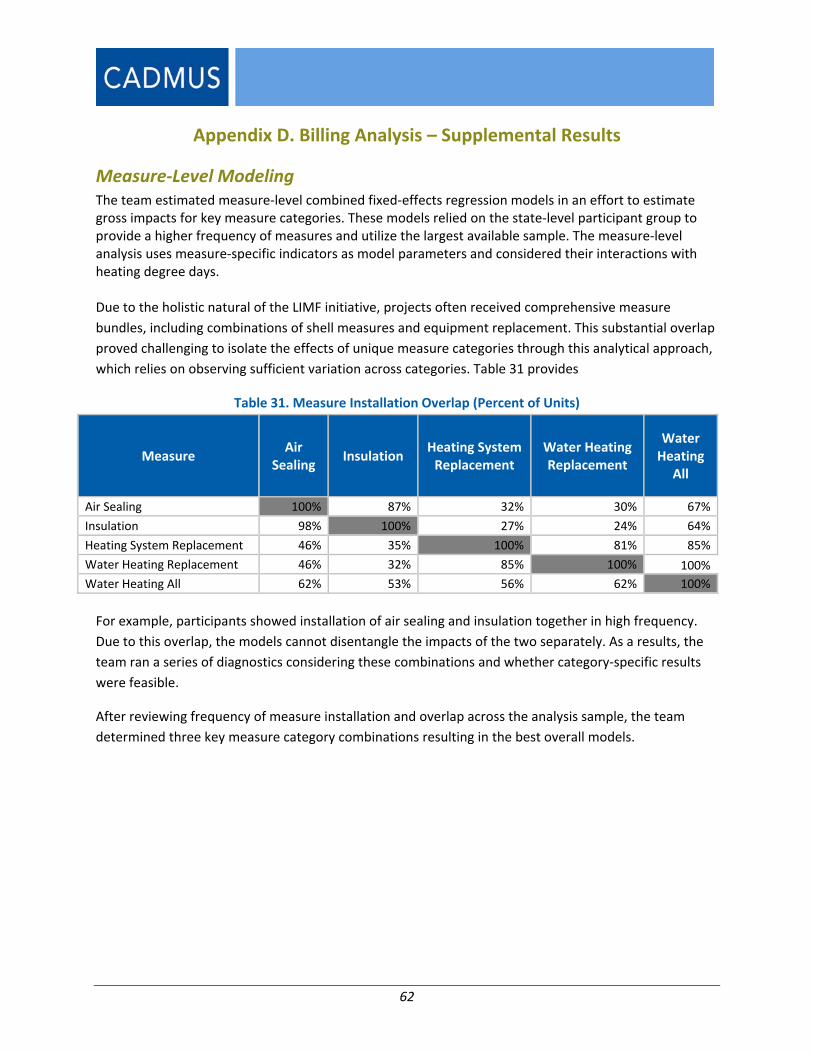
62 

Appendix D. Billing Analysis – Supplemental Results 

Measure‐Level Modeling The team estimated measure‐level combined fixed‐effects regression models in an effort to estimate gross impacts for key measure categories. These models relied on the state‐level participant group to provide a higher frequency of measures and utilize the largest available sample. The measure‐level analysis uses measure‐specific indicators as model parameters and considered their interactions with heating degree days.  Due to the holistic natural of the LIMF initiative, projects often received comprehensive measure 

bundles, including combinations of shell measures and equipment replacement. This substantial overlap 

proved challenging to isolate the effects of unique measure categories through this analytical approach, 

which relies on observing sufficient variation across categories. Table 31 provides  

Table 31. Measure Installation Overlap (Percent of Units)  

Measure Air 

Sealing Insulation 

Heating System Replacement 

Water Heating Replacement 

Water Heating 

All 

Air Sealing  100%  87% 32% 30%  67%

Insulation  98%  100% 27% 24%  64%

Heating System Replacement  46%  35% 100% 81%  85%

Water Heating Replacement  46%  32% 85% 100%  100% 

Water Heating All  62%  53% 56% 62%  100%

 For example, participants showed installation of air sealing and insulation together in high frequency. 

Due to this overlap, the models cannot disentangle the impacts of the two separately. As a results, the 

team ran a series of diagnostics considering these combinations and whether category‐specific results 

were feasible. 

After reviewing frequency of measure installation and overlap across the analysis sample, the team 

determined three key measure category combinations resulting in the best overall models.  

 

 

 

 

 

 

 

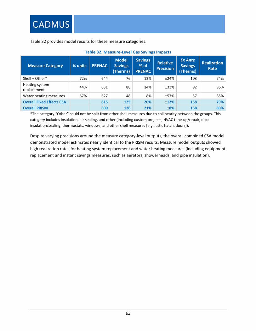
63 

Table 32 provides model results for these measure categories. 

Table 32. Measure‐Level Gas Savings Impacts 

Measure Category  % units  PRENAC Model Savings (Therms) 

Savings % of 

PRENAC 

Relative Precision 

Ex Ante Savings (Therms) 

Realization Rate 

Shell + Other*  72%  644 76 12% ±24% 103  74%

Heating system replacement 

44%  631 88 14% ±33% 92  96%

Water heating measures  67%  627 48 8% ±57% 57  85%

Overall Fixed Effects CSA     615 125 20% ±12% 158  79%

Overall PRISM     609 126 21% ±8% 158  80%

*The category “Other” could not be split from other shell measures due to collinearity between the groups. This 

category includes insulation, air sealing, and other (including custom projects, HVAC tune‐up/repair, duct 

insulation/sealing, thermostats, windows, and other shell measures [e.g., attic hatch, doors]). 

Despite varying precisions around the measure category‐level outputs, the overall combined CSA model 

demonstrated model estimates nearly identical to the PRISM results. Measure model outputs showed 

high realization rates for heating system replacement and water heating measures (including equipment 

replacement and instant savings measures, such as aerators, showerheads, and pipe insulation).