low frequency waves upstream and downstream of the
TRANSCRIPT

Low Frequency WavesUpstream and Downstream of
the Terrestrial Bow Shock
Von der Fakultat fur Physik und Geowissenschaften
der Technischen Universitat Carolo-Wilhelmina
zu Braunschweig
zur Erlangung des Grades eines
Doktors der Naturwissenschaften
(Dr.rer.nat.)
genehmigte
Dissertation
von Yasuhito Narita
aus Nagoya, Aichi, Japan

Bibliografische Information Der Deutschen Bibliothek
Die Deutsche Bibliothek verzeichnet diese Publikation in der DeutschenNationalbibliografie; detaillierte bibliografische Daten sind im Internetuberhttp://dnb.ddb.de abrufbar.
1. Referentin oder Referent: Prof. Dr. Karl-Heinz Glaßmeier
2. Referentin oder Referent: Prof. Dr. Uwe Motschmann
3. Referentin oder Referent: Prof. Dr. Toshifumi Mukai
eingereicht am: 26. Oktober 2005
mundliche Prufung (Disputation) am: 16. Februar 2006
Copyright c© Copernicus GmbH 2006
ISBN 3-936586-50-0
Copernicus GmbH, Katlenburg-Lindau
Druck: Schaltungsdienst Lange, Berlin
Printed in Germany

Vorabveroffentlichungen der Dissertation
Teilergebnisse aus dieser Arbeit wurden mit Genehmigung der Fakultat fur Physik undGeowissenschaften, vertreten durch den Mentor der Arbeit, in folgenden Beitragen vorabveroffentlicht:
Publikationen:
Narita, Y., K.-H. Glassmeier, S. Schafer, U. Motschmann, K. Sauer, I. Dandouras, K.-H. Fornacon, E. Georgescu und H. Reme, Dispersion analysis of ULF waves in theforeshock using cluster data and the wave telescope technique,Geophys. Res. Lett, 30,SSC 43-1, CiteID 1710, doi:10.1029/2003GL017432, 2003.
Narita, Y., K.-H. Glassmeier, S. Schafer, U. Motschmann, M. Franz, I. Dandouras, K.-H. Fornacon, E. Georgescu, A. Korth, H. Reme und I. Richter, Alfven waves in theforeshock propagating upstream in the plasma rest frame: statistics from Cluster ob-servations,Ann. Geophysicae, 22, 2315-2323, 2004.
Gurgiolo, C., M. L. Goldstein, Y. Narita, K.-H. Glassmeier und A. N. Fazakerley, A phaselocking mechanism for non-gyrotropic electron distributions upstream of the Earth’sbow shock,J. Geophys. Res., 110, A06206, doi:10.1029/2005JA011010, 2005.
Eastwood, J. P., E. A. Lucek, C. Mazelle, K. Meziane, Y. Narita, J. Pickett und R. A.Treumann, The foreshock,Space Sci. Rev., 118, 41-94, doi:10.1007/s11214-005-3824-3, 2005.
Narita, Y. und K.-H. Glassmeier Dispersion analysis of low-frequency waves through theterrestrial bow shock,J. Geophys. Res., 110, A12215, doi:10.1029/2005JA011256,2005.
Narita, Y. und K.-H. Glassmeier, Low-frequency waves in the bow shock environment,Proc. of the Cluster and Double Star Symposium - 5th Anniversary of Cluster in Space,(Ed) K. Fletcher, SP-598, ISBN 92-9092-909-X, ISSN 1609-042X, ESA PublicationsDivision, The Netherlands, January 2006.
Narita, Y., K.-H. Glassmeier, K.-H. Fornacon, I. Richter, S. Schafer, U. Motschmann, I.Dandouras, H. Reme und E. Georgescu, Low frequency wave characteristics in theupstream and downstream regime of the terrestrial bow shock,J. Geophys. Res., 111,A01203, doi:10.1029/2005JA011231, 2006.
3

Vorabveroffentlichungen der Dissertation
Narita, Y., K.-H. Glassmeier und R. A. Treumann, Magnetic turbulence spectra in thehigh-beta plasma upstream of the terrestrial bow shockPhys. Rev. Lett., eingereicht,2006.
Narita, Y., Low frequency waves upstream and downstream of the terrestrial bow shock,Planet. Space Sci., eingereicht, 2006.
Tagungsbeitrage:
AGU (Americal Geophysical Union) Fall Meeting 2002, San Francisco, Vereinigten Staa-ten von Amerika, 9. Dez. 2002 (Polarization and dispersion analysis of ULF wavesusing Cluster data, poster)
ISSI (International Space Science Institute) 1st Workshop on dayside magnetosphericboundaries, Bern, Schweiz, 19. Mar. 2003 (ULF wave analysis in the magnetosheathand upstream solar wind - short report from Braunschweig/FGM team, talk)
EGS-AGU-EUG Joint Assembly, Nizza, Frankreich, 7. Apr. 2003, (Wave propagatingdirections in the terrestrial magnetosheath, poster)
EGS-AGU-EUG Joint Assembly, Nizza, Frankreich, 8. Apr. 2003, (Dispersion Analysisand Wave Mode Identification of Magnetosheath Fluctuations: Is the MHD Assump-tion Justified? - A Case Study, talk)
STAMMS (Spatio-Temporal Analysis and Multi-point Measurements in Space), Orleans,Frankreich, 13. Mai 2003 (Application of wave telescope - foreshock wave study,poster)
IUGG (International Union of Geophysics and Geodesy) General Assembly 2003, Sap-poro, Japan, 30. Jun. 2003 (Dispersion analysis of ULF waves in the foreshock usingCluster data, talk)
ISSI 2nd Workshop on dayside magnetospheric boundaries, Bern, Schweiz, 12. Nov.2003 (Wave modes and large scale wave distribution -1. foreshock, - 2. magnetosheath,talks)
EGU (European Geosciences Union) General Assembly, Nizza, Frankreich, 30. Apr.2004 (Dispersion relation and wave propagation in the foreshock and magnetosheath:Low-frequency picture from Cluster, poster)
Cluster FGM Workshop, London, Großbritanien, Mar. 2005, (Low frequency waves up-stream and downstream of the bow shock, talk)
Magnetometer workshop, Ibenhorst, Born, Deutschland, 12. Apr. 2005, (Low frequencywaves upstream and downstream of the bow shock, talk)
EGU General Assembly, Wien,Osterreich, 29. Apr. 2005, (A statistical picture of low
4

Vorabveroffentlichungen der Dissertation
frequency waves from the upstream to the downstream region of the terrestrial bowshock - Cluster observations, talk)
IAGA (International Association of Geomagnetism and Aeronomy) Scientific Assembly,Toulouse, Frankreich, 20. Jul. 2005 (Evidence of low frequency turbulence in thenear-Earth solar wind plasma, talk)
STIMGM Workshop (Solar - Terrestrial Interactions from Microscale to Global Models),Sinaia, Rumanien, 9. Sep. 2005 (Magnetic turbulence, talk; Low-frequency waves inthe magnetosphere - a view from multi-point measurements, invited talk)
Cluster and Double Star symposium - 5th anniversary of Cluster in Space, ESTEC, No-ordwijk, Niederlande, 21. Sep. 2005, (Low frequency waves in the bow shock envi-ronment, poster)
SGEPSS (Society of Geomagnetism and Earth, Planetary and Space Sciences, Japan)annual meeting, Kioto, Japan, 29. und 30. Sep. 2005, (Low frequency waves in thebow shock environment, talk; Magnetic turbulence spectra, poster)
Evaluation Meeting of the International Max Planck Research School, Katlenburg-Lindau,11. Nov. 2005, (Bow shock upstream and downstream waves, talk)
5


Contents
Vorabveroffentlichungen der Dissertation 3
Summary 17
1 Introduction 191.1 Space plasma . . . . . . . . . . . . . . . . . . . . . . . . . . . . . . . .191.2 Waves and instabilities . . . . . . . . . . . . . . . . . . . . . . . . . . .201.3 Shock waves . . . . . . . . . . . . . . . . . . . . . . . . . . . . . . . .201.4 Upstream and downstream waves . . . . . . . . . . . . . . . . . . . . . .21
2 Shocks, upstream and downstream waves, turbulence 232.1 Collisionless shocks . . . . . . . . . . . . . . . . . . . . . . . . . . . . .23
2.1.1 Rankine-Hugoniot relations . . . . . . . . . . . . . . . . . . . .242.1.2 Different types of shocks . . . . . . . . . . . . . . . . . . . . . .262.1.3 Bow shock . . . . . . . . . . . . . . . . . . . . . . . . . . . . .28
2.2 Upstream waves . . . . . . . . . . . . . . . . . . . . . . . . . . . . . . .312.2.1 Ion beam instabilities . . . . . . . . . . . . . . . . . . . . . . . .322.2.2 Shock foot waves . . . . . . . . . . . . . . . . . . . . . . . . . .33
2.3 Downstream waves . . . . . . . . . . . . . . . . . . . . . . . . . . . . .342.3.1 Ion cyclotron instability . . . . . . . . . . . . . . . . . . . . . .342.3.2 Mirror instability . . . . . . . . . . . . . . . . . . . . . . . . . .35
2.4 Turbulence . . . . . . . . . . . . . . . . . . . . . . . . . . . . . . . . .352.4.1 Hydrodynamic turbulence . . . . . . . . . . . . . . . . . . . . .362.4.2 Magnetohydrodynamic turbulence . . . . . . . . . . . . . . . . .382.4.3 Intermittency . . . . . . . . . . . . . . . . . . . . . . . . . . . .402.4.4 Turbulence in space . . . . . . . . . . . . . . . . . . . . . . . . .40
3 In-situ wave observations 433.1 The Cluster mission . . . . . . . . . . . . . . . . . . . . . . . . . . . . .433.2 FGM . . . . . . . . . . . . . . . . . . . . . . . . . . . . . . . . . . . . .433.3 CIS . . . . . . . . . . . . . . . . . . . . . . . . . . . . . . . . . . . . .473.4 PEACE . . . . . . . . . . . . . . . . . . . . . . . . . . . . . . . . . . .513.5 Wave analyses . . . . . . . . . . . . . . . . . . . . . . . . . . . . . . . .51
7

Contents
3.5.1 Frequency and wave power . . . . . . . . . . . . . . . . . . . . .53
3.5.2 Ellipticity . . . . . . . . . . . . . . . . . . . . . . . . . . . . . .53
3.5.3 Minimum variance analysis . . . . . . . . . . . . . . . . . . . .54
3.5.4 Correlation and coherence . . . . . . . . . . . . . . . . . . . . .54
3.5.5 Wave vector . . . . . . . . . . . . . . . . . . . . . . . . . . . . .55
3.5.6 Frequency and phase velocity in the plasma rest frame . . . . . .57
3.5.7 Dispersion relation and propagation pattern . . . . . . . . . . . .57
4 Dispersion analysis of upstream waves 594.1 Introduction . . . . . . . . . . . . . . . . . . . . . . . . . . . . . . . . .59
4.2 Dispersion analysis . . . . . . . . . . . . . . . . . . . . . . . . . . . . .59
4.3 Dispersion in a beam plasma . . . . . . . . . . . . . . . . . . . . . . . .63
4.4 Discussion . . . . . . . . . . . . . . . . . . . . . . . . . . . . . . . . . .64
4.5 Summary . . . . . . . . . . . . . . . . . . . . . . . . . . . . . . . . . .65
5 Wave-particle interaction in the upstream region 675.1 Introduction . . . . . . . . . . . . . . . . . . . . . . . . . . . . . . . . .67
5.2 Wave analysis . . . . . . . . . . . . . . . . . . . . . . . . . . . . . . . .67
5.3 Phase-bunched electrons . . . . . . . . . . . . . . . . . . . . . . . . . .70
5.4 Discussion . . . . . . . . . . . . . . . . . . . . . . . . . . . . . . . . . .74
5.5 Summary . . . . . . . . . . . . . . . . . . . . . . . . . . . . . . . . . .75
6 Statistical study of upstream waves 776.1 Introduction . . . . . . . . . . . . . . . . . . . . . . . . . . . . . . . . .77
6.2 Case study . . . . . . . . . . . . . . . . . . . . . . . . . . . . . . . . . .77
6.3 Statistical study . . . . . . . . . . . . . . . . . . . . . . . . . . . . . . .82
6.4 Discussion . . . . . . . . . . . . . . . . . . . . . . . . . . . . . . . . . .86
6.5 Summary . . . . . . . . . . . . . . . . . . . . . . . . . . . . . . . . . .87
7 Dispersion analysis of downstream waves 917.1 Introduction . . . . . . . . . . . . . . . . . . . . . . . . . . . . . . . . .91
7.2 Dispersion analysis . . . . . . . . . . . . . . . . . . . . . . . . . . . . .93
7.3 Discussion . . . . . . . . . . . . . . . . . . . . . . . . . . . . . . . . . .96
7.4 Summary . . . . . . . . . . . . . . . . . . . . . . . . . . . . . . . . . .99
8 Statistical study of downstream waves 1018.1 Introduction . . . . . . . . . . . . . . . . . . . . . . . . . . . . . . . . .101
8.2 Statistical study . . . . . . . . . . . . . . . . . . . . . . . . . . . . . . .101
8.3 Results . . . . . . . . . . . . . . . . . . . . . . . . . . . . . . . . . . . .108
8.4 Discussion . . . . . . . . . . . . . . . . . . . . . . . . . . . . . . . . . .116
8.5 Summary . . . . . . . . . . . . . . . . . . . . . . . . . . . . . . . . . .121
8

Contents
9 Magnetic turbulence 1319.1 Introduction . . . . . . . . . . . . . . . . . . . . . . . . . . . . . . . . .1319.2 Dispersion curves andk-spectra . . . . . . . . . . . . . . . . . . . . . .1329.3 Discussion . . . . . . . . . . . . . . . . . . . . . . . . . . . . . . . . . .1379.4 Summary . . . . . . . . . . . . . . . . . . . . . . . . . . . . . . . . . .139
10 Summary and outlook 141
Acknowledgments 159
Curriculum Vitae 163
9


List of Figures
2.1 Fast and slow shock wave . . . . . . . . . . . . . . . . . . . . . . . . . .252.2 Quasi-parallel and quasi-perpendicular shock . . . . . . . . . . . . . . .262.3 Magnetic field profiles across shocks . . . . . . . . . . . . . . . . . . . .282.4 Earth’s bow shock and magnetosphere . . . . . . . . . . . . . . . . . . .292.5 Hubble Space Telescope image of a bow shock . . . . . . . . . . . . . .302.6 Image of turbulent water jet . . . . . . . . . . . . . . . . . . . . . . . . .362.7 Kolmogorov energy spectrum . . . . . . . . . . . . . . . . . . . . . . . .382.8 Images of examples of interstellar turbulence . . . . . . . . . . . . . . .39
3.1 Artist’s impression of the Cluster spacecraft . . . . . . . . . . . . . . . .443.2 Image of the Cluster spacecraft . . . . . . . . . . . . . . . . . . . . . . .453.3 Basic components of a fluxgate magnetometer . . . . . . . . . . . . . . .463.4 Image of Cluster FGM . . . . . . . . . . . . . . . . . . . . . . . . . . .473.5 Image of CODIF and HIA sensor . . . . . . . . . . . . . . . . . . . . . .483.6 Basic components of HIA . . . . . . . . . . . . . . . . . . . . . . . . . .493.7 Basic components of CODIF . . . . . . . . . . . . . . . . . . . . . . . .503.8 Basic components of PEACE . . . . . . . . . . . . . . . . . . . . . . . .513.9 Image of PEACE LEEA . . . . . . . . . . . . . . . . . . . . . . . . . .523.10 Image of PEACE HEEA . . . . . . . . . . . . . . . . . . . . . . . . . .523.11 Wave power distributions ink-domain . . . . . . . . . . . . . . . . . . . 57
4.1 Magnetic field and plasma profile in the foreshock . . . . . . . . . . . . .604.2 Dispersion relations in three components . . . . . . . . . . . . . . . . . .614.3 Comparison of dispersion relations . . . . . . . . . . . . . . . . . . . . .624.4 Ion velocity distribution . . . . . . . . . . . . . . . . . . . . . . . . . . .64
5.1 Magnetic field oscillation upstream of the bow shock . . . . . . . . . . .685.2 Dynamic wave power spectrograms . . . . . . . . . . . . . . . . . . . .695.3 Wave power in frequency and wave number domain . . . . . . . . . . . .705.4 Hodograms of magnetic field oscillation . . . . . . . . . . . . . . . . . .715.5 Phase-elevation plots showing nongyrotropic electrons . . . . . . . . . .715.6 PEACE measurement matrix . . . . . . . . . . . . . . . . . . . . . . . .735.7 Phase angle evolution of nongyrotropic electons . . . . . . . . . . . . . .74
11

List of Figures
6.1 Magnetic field and plasma profile across the bow shock . . . . . . . . . .786.2 Configuration of foreshock wave observation . . . . . . . . . . . . . . .806.3 Power spectrum in frequency domain . . . . . . . . . . . . . . . . . . .816.4 Wave power ink-space . . . . . . . . . . . . . . . . . . . . . . . . . . .826.5 Histogram of wave number . . . . . . . . . . . . . . . . . . . . . . . . .836.6 Spatial distribution of wave phase velocities . . . . . . . . . . . . . . . .846.7 Foreshock wave properties . . . . . . . . . . . . . . . . . . . . . . . . .86
7.1 Magnetic field and plasma profile across the bow shock . . . . . . . . . .927.2 Cluster orbit . . . . . . . . . . . . . . . . . . . . . . . . . . . . . . . . .937.3 Dispersion relations and propagation angles in the upstream and the down-
stream region. . . . . . . . . . . . . . . . . . . . . . . . . . . . . . . . .957.4 Histograms of magnetic field polarization . . . . . . . . . . . . . . . . .967.5 Schematic illustration of wave habitats . . . . . . . . . . . . . . . . . . .98
8.1 Magnetic field and plasma profile across the bow shock . . . . . . . . . .1028.2 Sketches of the solar wind coordinate system . . . . . . . . . . . . . . .1048.3 Cluster orbit in the solar wind coordinate system . . . . . . . . . . . . .1058.4 Wave power in frequency domain . . . . . . . . . . . . . . . . . . . . .1068.5 Magnetic field and ion number density profile . . . . . . . . . . . . . . .1068.6 Wave power ink-space . . . . . . . . . . . . . . . . . . . . . . . . . . .1078.7 Histograms of frequencies . . . . . . . . . . . . . . . . . . . . . . . . .1088.8 Histograms of wave numbers divided by ion inertial wave number . . . .1098.9 Histograms of wave numbers divided by thermal ion gyro-wave number .1108.10 Histograms of phase velocities divided by fast mode speed . . . . . . . .1108.11 Histograms of phase velocities divided by intermediate mode speed . . .1118.12 Histograms of phase velocities divided by slow mode speed . . . . . . . .1118.13 Histograms of propagation angles . . . . . . . . . . . . . . . . . . . . .1128.14 Histograms of magnetic polarization . . . . . . . . . . . . . . . . . . . .1128.15 Histograms of phase angles between plasma density and magnetic field
strength variations . . . . . . . . . . . . . . . . . . . . . . . . . . . . . .1138.16 Histograms of phase angles between plasma bulk velocity and magnetic
field variations . . . . . . . . . . . . . . . . . . . . . . . . . . . . . . . .1138.17 Distributions of mean magnetic field, plasma density and temperature . .1148.18 Distributions of propagation angles, phase velocities, and phase angles
between plasma density and magnetic field variations . . . . . . . . . . .1158.19 Spatial distribution of phase velocities in the GSE coordinate system . . .1178.20 Spatial distribution of phase velocities in the solar wind system . . . . . .1188.21 Sketch of propagation pattern . . . . . . . . . . . . . . . . . . . . . . . .1198.22 Histograms of relative errors . . . . . . . . . . . . . . . . . . . . . . . .120
9.1 Dispersion relation andk-spectra . . . . . . . . . . . . . . . . . . . . . .1339.2 Comparison ofk-spectra between direct and indirect measurements . . .135
12

List of Figures
9.3 Dispersion relation andk-spectra for non-compressive components . . . .1369.4 Dispersion relation andk-spectra for compressive components . . . . . .1379.5 Probability distribution functions . . . . . . . . . . . . . . . . . . . . . .138
10.1 Cluster magnetic field investigators . . . . . . . . . . . . . . . . . . . . .160
13


List of Tables
6.1 Time intervals and frequencies of foreshock waves . . . . . . . . . . . .88
7.1 Plasma parameterβ, temperature anisotropy, and transport ratio . . . . .97
8.1 Time intervals and frequencies of magnetosheath waves . . . . . . . . . .1238.2 Time intervals and frequencies of quasi-perpendicular shock upstream
waves . . . . . . . . . . . . . . . . . . . . . . . . . . . . . . . . . . . .129
15


Summary
Studying space plasmas is of significant importance not only in geophysical or space re-search, but also with respect to the fundamental physics of collisionless plasmas. It hasbeen suspected since the days of the early development of plasma physics that collision-less plasmas exhibit numerous kinds of waves and instabilities, but it is rare to unambigu-ously identify them in experiments in spite of a number of in-situ spacecraft measurementsfor decades. Our knowledge about space plasmas is still limited. One of the difficultiesin understanding space plasma phenomena stems from the fact that the experiments weremade using single or at best double spacecraft measurements. It is not easy in spaceunless having any assumptions to distinguish spatial variations from temporal variationsfrom only one or two point measurements. Spatial scales like wavelengths are not yetinvestigated in space. It was not until the advent of Cluster, four spacecraft mission, thatone measures space plasma at last with spatial resolution in three dimensions.
The solar wind interacts with the Earth’s magnetic field in various ways includingwaves. The existence of waves upstream and downstream of the bow shock ahead ofthe Earth have been known since the discovery of the bow shock and various kinds ofplasma models and ideas were proposed to understand the nature of these waves. Studyingthe Earth’s bow shock and its associated wave activity is important, for it is the onlyaccessible collisionless shock for detailed investigations and has immediate astrophysicalimplications.
This PhD thesis presents the analysis of low frequency waves upstream and down-stream of the terrestrial bow shock, taking advantage of the four point measurements, andcontributes to fundamental plasma physics as well as the research of Sun-Earth interac-tion. The thesis first reviews our current understanding about the bow shock, upstreamand downstream waves and turbulence in Chapter 2 and introduces the experiment usingCluster and wave analysis methods in Chapter 3.
Chapter 4 presents a dispersion analysis of the upstream waves. The wave dispersionrelation is determined experimentally and shows a good agreement with the one calculatedfor the ion beam plasma model, suggesting that the upstream waves represent whistler andbeam resonant waves. This is one of examples of wave mode identification and confirmsthe physical processes drawn by the earlier studies that some upstream ions are specularlyreflected at the shock and flow against the incoming ions, while they form an unstableparticle distribution in velocity space which drives waves and collapses into a stable state.
Chapter 5 presents an example of wave-particle interaction. The dispersion and polar-
17

Summary
ization analysis indicate the existence of the whistler wave in the upstream region. Thewave is accompanied by nongyrotropic electrons which are trapped by the wave field.While it is known that some beam ions are phase bunched by the wave field, there is alsoan interplay between the waves and the electrons.
Chapter 6 presents a statistical study of the upstream waves. It is shown that the wavephase velocities in the plasma rest frame of reference are oriented toward upstream alongthe magnetic field. This direction is the same as that of the backstreaming ions.
Chapter 7 presents the dispersion analysis of the downstream waves. The dispersioncurves are investigated along a Cluster orbit and show a transition from the whistler andthe beam resonant waves in the upstream region to the mirror mode in the downstreamregion. The upstream waves are not transmitted across the shock, as they are swept by thesolar wind toward downstream.
Chapter 8 presents a statistical study of the downstream waves. While the upstreamwaves propagate parallel to the background magnetic field, the downstream waves propa-gate perpendicular. The mirror mode properties are frequently detected in the downstreamregion but they have finite propagation speed, possibly coupled to the background inho-mogeneities or nonlinear effects. On the statistical average there is an organization inwave propagation pattern: outward divergent in the upstream region; toward the magne-tosheath flank region aligned with the plasma flow direction in the downstream region;and inward convergent in the magnetosheath flank.
Chapter 9 attempts to determine the spectra of magnetic turbulence directly in thewave number domain. The direct determination has been done for the first time in spaceplasma. The spectra for the upstream waves show three ranges: the injection range iden-tified at small wave numbers with the wave coupling region between the whistler and thebeam resonant mode wave, the quasi-inertial range, and the dissipation range. The fluc-tuations exhibit properties of not fully developed turbulence but intermittency, suggestingthat there is not enough time for turbulence to become fully developed.
The above results indicate that disturbances in the plasma caused by the bow shocklead to wave excitation both in the upstream and the downstream regions, but the waveproperties are different between them and accordingly the physical processes are different.The upstream waves propagate parallel to the magnetic field and are identified as the onedriven by the ion beam instability, while the downstream waves propagate perpendicularand represent the mirror modes. On the other hand they exhibit a unique propagationpattern imposed by the background magnetic field topology in those regions. Multi-pointmeasurements are essential in understanding waves, instabilities, and turbulence in space.
18

1 Introduction
1.1 Space plasma
A plasma is an ionized gas and often called the fourth state of matter. It is realized whenthe temperature of the matter is so high that the atoms dissociate into ions and electrons.The plasma behaves considerably different from what we know about the matter on theground of the Earth. Since it is an electrically conductive medium and capable of carryingelectric currents, it is not simply described by the laws of gas or fluid dynamics. It reactssensitively to electric and magnetic fields and disturbs those fields due to the currentsin it which complicates us to comprehend its behavior correctly. With the advent of thespaceflight era the interests of geophysicists are oriented not only into the Earth’s internalstructure and its dynamics but also the neighboring environment about the Earth and itwas understood that the neighborhood is in an ionized state. Today it is widely believedthat most of the baryonic matters in the Universe is in the plasma state. Space physics istherefore to a large part plasma physics.
There are different kinds of plasmas. The plasmas are characterized into, for example,collisional or collisionless plasmas, dense or dilute plasmas, hot or cold plasmas, mag-netized or unmagnetized plasmas, fully or partially ionized gas, and so on. To specifythe plasma temperature, the plasma parameterβ is often introduced which is a ratio ofthermal to magnetic field energy density. What characterizes the space plasma uniquelyis the absence of particle collisions. Too huge system size and too small particle den-sity make it hard to achieve laboratory experiments on the ground. Instead, the use ofspacecraft has been enabling the physicists to makein situ experiments in the near Earthspace, which is the only accessible collisionless plasma to us. One may regard that thenear Earth space plasma serves as a natural laboratory and expect to apply the results toastrophysical phenomena.
Plasmas in space are in many situations accompanied by electromagnetic fields. Plas-mas are electrically quasi-neutral, as the electric charge in each volume element is shieldedby oppositely charged particles. But electric fields may arise in plasmas, for example,when plasmas flow in magnetic fields, they generate convective electric fields. Magneticfields may also arise due to so-called dynamo processes. Magnetic fields in the plasmaare subject to two effects, depending on the electric conductivity of the plasma. Theydiffuse under the low conductivity; or they are “frozen-in” to the plasma under the highconductivity, which means that the fields are carried by the plasma flow. For instance,
19

1 Introduction
the plasma in the interplanetary space is characterized by a very high conductivity andthe interplanetary magnetic field is carried by the solar wind plasma away from the sun.In space it is possible that the energy density of electromagnetic fields exceeds kineticor thermal energy of the plasmas. Furthermore, plasmas allow processes that exchangedifferent kinds of energies between one another. The kinetic energy can be converted intothe magnetic field energy by the dynamo processes, and on the other hand the magneticfield energy can be converted back into the kinetic energy by the reconnection processes.The electromagnetic fields play therefore an important role as well as the plasma itself.
1.2 Waves and instabilities
The collisionless nature of space plasma indicates that unstable configurations in the senseof ordinary gas dynamics such as the temperature anisotropy, beams, and temperature dif-ference among species are preserved in principle. Charged particles, however, interactwith one another remotely via disturbances of the electric and the magnetic fields. Thespace plasmas exhibit in many cases dynamic and transient phenomena. As they areelectrically conducting, their dynamic motions are accompanied by magnetic field fluc-tuations. While an ordinary gas permits solely sound waves propagating in the medium,plasmas exhibit numerous kinds of waves propagating. Electric currents in the plasmareact to the wave electric and magnetic fields in various ways depending on scales andfrequencies of interest, which results in distortion or introduction of restoration force.The plasmas also allow many kinds of instabilities to exist, in which case the restorationforce in the disturbance reacts positively in such a way that the disturbance grows. Theplasmas can distribute energy and momentum to bring the system toward an equilibriumby means of waves and instabilities.
1.3 Shock waves
Boundaries are often formed in space when different kinds of plasmas meet each other.For example, the interaction of the solar wind with the Earth’s magnetic field results in theformation of a magnetospheric cavity bounded by the magnetopause. The solar wind is aplasma stream arising from the solar corona. Since the solar wind flows faster than anywave propagation speeds allowed, a standing shock wave (bow shock) is formed ahead ofthe Earth as it meets the Earth as an obstacle. The interaction also results in the formationof a boundary separating the solar wind plasma from the Earth ionospheric and magne-tospheric plasmas called themagnetopause. Other types of boundaries may exist in theplasma in general. They are classified based on the conservation laws across discontinu-ities in the ideal magnetohydrodynamical picture (theRankine-Hugoniot relations). Theshock wave solution is also derived from the Rankine-Hugoniot relations. In the gas dy-namics a shock wave comes about when a supersonic flow meets an obstacle and particlescollide suddenly. A similar situation can be found in the plasma though particles remain
20

1.4 Upstream and downstream waves
collisionless. For this to happen, the flow speed must exceed not the sound speed butthe magnetosonic speedwhich is determined by the magnetic field, the plasma density,the temperature, and the propagation direction. A sudden compression of the magneticfield and the plasma is accompanied when the plasma undergoes the shock. Structure,dynamics of the shock, and dissipation process are known to be sensitively dependent onthe upstream states such as the magnetic field geometry, the upstream flow velocity, andthe plasma parameterβ. The collisionless shocks under some conditions are markedlycharacterized by a specular reflection of particles at the shock such that a portion of theupstream particle population gains energy at the shock and streams against the incomingflow toward upstream. The backstreaming particles, while interacting with the upstreamflow, form a unique region ahead of the shock called theforeshock. Such a situation isnever found in the ordinary gas dynamics nor in the fluid dynamics.
1.4 Upstream and downstream waves
Since the first spacecraft detected the existence of the shock wave ahead of the Earth ithas been known that the upstream and the downstream plasmas exhibit moderate to highlevel of magnetic field and plasma fluctuations, indicating that the shock formation isaccompanied by some wave processes ahead of and behind the shock. Many theoreticaland experimental attempts have been made to understand the physics of the upstream andthe downstream waves. However, it is not easy to investigate wave properties in a properframe of reference, theplasma rest frame, because one can not distinguish between spatialand temporal variations from the acquired spacecraft data. This problem reflects the factthat the waves are Doppler shifted as the background medium sweeps the waves andmodulates wave frequencies. Using single spacecraft, it is impossible to determine howmuch the frequency detected comes from the convection part and how much from theintrinsic one. There were double spacecraft missions but only one dimensional spatialscale was obtained and one must have a good condition that the wave propagation isaligned with the spacecraft separation direction.
Acquisition of spatial resolution in three dimensions have remained as a task eversince the earliest spacecraft missions. With the advent of the Cluster mission, consistingof four spacecraft, the spatial resolution has at last become available atin situ observa-tions. Having speculations and scenarios derived from the early spacecraft observationsand theoretical studies in mind, this thesis aims to reveal the nature of the upstream andthe downstream waves.
This thesis is organized in the following fashion. Chapter 2 introduces the conceptof a collisionless shock. Foundations of the shock, theories, and observations about theupstream and the downstream waves are reviewed. Chapter 3 describes an outline of theCluster mission and instrumentation for the magnetic field and the plasma measurements.
21

1 Introduction
The wave analysis methods are presented, too. Chapter 4 and 5 present dispersion analy-ses of the upstream waves, where wave dispersion relations are determined experimentallyand compared to theoretical dispersion curves. Chapter 6 presents a statistical study ofthe upstream waves. Chapter 7 presents a dispersion analysis of the downstream waves.The dispersion curves are investigated along a spacecraft orbit and compared with theupstream case. Chapter 8 presents a statistical study of the downstream waves. Chapter9 attempts to determine directly turbulence spectra of magnetic field fluctuations for theupstream waves.
22

2 Shocks, upstream and downstreamwaves, turbulence
2.1 Collisionless shocks
Most of our everyday notions of the nature of shock waves (or simply shocks) come fromour experience of supersonic aircraft or explosive blasts. The study of shocks began withordinary gas dynamics in the late 19th century and reached its maturity during the 1940s,at the time of the development of high-performance aircraft. The study of plasma shockssurfaced during the 1950s. Earlier, it was debated whether collisionless shock waves evenexisted. Some argued that the rarity of collisions in a high temperature plasma precludedthe existence of shocks, while others maintained that collective micro-turbulence wouldreplace particle collisions to create a shock with a thickness much less than a collisionmean free path. The solar wind proved, upon its discovery in 1959-1963, to have a fastflow speed and an enormous mean free path which is comparable to the distance from theEarth to the sun. Since it had been difficult to make collision-free plasmas in the labora-tory, some foresaw that the first collisionless shock would be discovered in space. Andso it was, standing in the solar wind in front of the Earth’s magnetosphere called thebowshock(Sonett and Abrams1963,Ness et al.1964). Also, high-altitude nuclear explosionsin the upper atmosphere and magnetic pinch fusion research motivated laboratory inves-tigations of the collisionless shocks. There was a good collaboration between laboratoryand space experimentalists, theoreticians, and specialists in numerical simulation. Afterthe collaboration ended in 1970s, when the interest in the magnetic pinch fusion wanedand financial support for the laboratory experiments disappeared, the space communitywas left to its own devices. Nowadays the space community plays a dominant role in thecollisionless shock research. The ISEE spacecraft (Ogilvie et al.1977) was well suited todetailed research of the collisionless shocks. The use of two spacecraft made it possibleto measure scale length, easy to do in laboratories but difficult in space. The discoveryof the Earth’s bow shock and the subsequent observations of planetary bow shocks andinterplanetary shocks have now firmly established that shocks can be produced in thecollisionless plasma. Space plasmas exhibit both stationary shocks like bow shocks pro-duced by the solar wind interaction with planets and transient shocks like solar flares andsupernova explosions.
Formation of a shock can be explained in terms of steepening of a large amplitude
23
2 Shocks, upstream and downstream waves, turbulence
wave. Such a wave is nonlinear, behaves like a soliton, and can steepen because the wavespeed with a shorter wavelength could be changed by the wave itself, which becomes thebasis of the shock. Nonlinear waves generally bear some resemblance to more familiarlinear modes and have a velocity typically equal to that of their corresponding linear modeand a wavelength at which the wave mode becomes dispersive (Krall 1997). This wouldeventually lead to sharp gradients and shock formation. When dissipation is present, thesolitons interact with the background medium as they propagate, so that the backgroundstate is changed by the solitons. For a shock to be stable, the wave steepening must bebalanced against the dissipation.
In collision dominated gases, the shock wave forms when the relative speed betweenthe flow and the obstacle exceeds the sound speed. The flow energy is dissipated by bi-nary collisions which lead to viscosity and friction. The ratio of the flow speed to thesound speed is called theMach number, M . The upstream region is characterized byM > 1 (supersonic flow) and low entropy, while the downstream region is characterizedbyM < 1 (subsonic flow) and high entropy, density, and pressure. The transition acrossa shock occurs in a distance of the order of a few collision mean free paths. In a collision-less plasma such as the solar wind the distance of even a few collisional mean free paths isvery large, and other processes intervene to control the thickness of such shocks. Energyand momentum can be transferred among particles via electric and magnetic field oscil-lations. These collective motions add to a rich variety of possible shocks and dissipationmechanisms. For instance, at the larger Mach numbers, thermal spread in the plasma al-lows particle reflection at the shock, which provides an additional dissipation mechanism.The situation becomes further complicated due to the fact that there are several propa-gation speeds allowed in the plasma. In magnetohydrodynamics (MHD), the one-fluidpicture of plasmas, there are three fundamental waves: fast, intermediate (Alfven), andslow modes. Because they have different characteristic propagation speeds, there are dif-ferent shocks which inherit some properties of corresponding wave modes. The structure,dynamics, and dissipation mechanism of the collisionless shocks are generally dependenton the magnetic field geometry with respect to the shock normal, the Mach number, andthe plasma parameterβ (ratio of thermal to magnetic pressure).
2.1.1 Rankine-Hugoniot relations
No matter how a shock is structured and organized, one knows that mass, energy, and mo-mentum must be conserved. One can then apply the conservation laws of MHD to relatethe downstream state with the upstream one and find possible solutions of the shocks. Inthe case of an ordinary gas, these relations were first derived by Rankine and Hugoniottoward the end of 19th century. The Rankine-Hugoniot relations determine uniquely thedownstream state in terms of the upstream states. Thus the shock structure is determinedonly by the dissipation mechanism, viscosity, which produces a shock with a thickness ofa few mean free paths. In the case of a collisionless plasma, the conservation laws (alsocalled the Rankine-Hugoniot relations) do not provide a unique relationship between the
24

2.1 Collisionless shocks
ShockUpstream Downstream
Magnetic Field
FastMode
SlowMode
Figure 2.1: Sketch of magnetic fields across a fast and a slow shock wave (afterBaumjo-hann and Treumann1997).
upstream and the downstream state. The Rankine-Hugoniot relations allow generally notonly shocks but also discontinuities to exist (Baumjohann and Treumann1997).
As mentioned above, three kinds of shocks exist from the viewpoint of the MHDconservation laws: fast, intermediate, and slow shocks. The fast and the slow shock havethe same behavior in terms of the plasma and magnetic pressure as the corresponding fastand slow mode waves in MHD. Across the fast shock, the magnetic pressure increasestogether with the plasma pressure. The normal component of the magnetic field to theshock is constant and the increase is seen only in the transversal component. Therefore,the downstream magnetic field is bent away from the shock normal (Fig. 2.1). In contrast,the magnetic pressure downstream of the slow shock decreases and the field is bent towardthe shock normal. Observationally, the fast shocks are the most frequent type in the solarsystem such as planetary bow shocks and interplanetary shocks. The slow shocks arerarer, but they have been observed and appear in some theories of magnetic reconnection.
The fast and slow shocks exhibit an interesting property called thecoplanarity theoremthat the upstream and downstream magnetic field directions and the shock normal all liein the same plane (Baumjohann and Treumann1997). The intermediate shock is a specialcase. In an isotropic plasma it is not a shock but called arotational discontinuity, acrosswhich there is a flow but no compression of the plasma or dissipation. Our discussionlater concentrates on the fast shocks.
25

2 Shocks, upstream and downstream waves, turbulence
ShockUpstream Downstream
Quasi-parallel shock
θ Bn
θ Bn < 45°
Quasi-perpendicular shock
θ Bn
θ Bn > 45°
ShockUpstream Downstream
Magnetic field
Shock normal
Figure 2.2: Sketch of magnetic fields across a quasi-parallel and a quasi-perpendicularshock (afterBaumjohann and Treumann1997,Schwartz2000).
2.1.2 Different types of shocks
There are many different types of shocks even if we restrict ourselves to the fast shocks.At all planetary bow shocks we find different structures. Early on there were debateswhether or not such shocks were actually stable. Perhaps all the different profiles seen inobservations were just fleeting glimpses of an ever-changing entity. A major contributionfrom the observations was the demonstration that there was a definite pattern of shocksdetermined by the complete set of upstream parameters. The most important factor incontrolling the type of shock is the direction of the upstream magnetic field relative to theshock normal. Depending on the value ofθBn which is the angle between the magneticfield direction and the shock normal, shocks are classified asparallel shocks(θBn = 0),asperpendicular shocks(θBn = 90), or asoblique shocks(0 < θBn < 90). One alsospeaks ofquasi-parallel shocks(θBn < 45) andquasi-perpendicular shocks(θBn > 45).Fig. 2.2 shows the quasi-parallel and the quasi-perpendicular shock. The distinctionbetween the two shocks is physically relevant. The perpendicular shocks are based on thefast magnetosonic waves, and the parallel shocks are based on the whistler waves (Krall1997). When the plasma becomes so hot that the magnetic field can be ignored, both thewaves degenerate into the ion acoustic wave and shocks become the hydrodynamic shock.
Particle dynamics is as important as the fluid picture to understand the shocks. Theions and electrons encountering the compressed magnetic field at the shock have differentgyroradii. The ions can penetrate deeper into the field than the electrons, because theions have larger mass. This difference in penetration depth generates a charge separationelectric field in the shock normal direction, pointing toward upstream. The electric fieldthen reflects a number of ions back into the upstream region, while it attracts and capturesthe electrons.
Shocks also depend on the Mach number and the plasmaβ. In the collisionlessplasma, shock heating must use mechanisms unique to plasmas. In the case of the low
26

2.1 Collisionless shocks
Mach number shocks (calledsubcritical shocks), mixing of the upstream flow and theplasma reflected from the obstacle causes a beam-beam instability. This results in Jouleheating due to the generation of anomalous collisions via field oscillations and resistivityin the current layer inside the shock. The heat is produced depending on the current inthe plasma. The instability and field fluctuation also cause an effective viscous interactionin the shock front and produce heat depending on the velocity gradient. In both caseswaves and instabilities replace collisions to scatter particles. These processes run rela-tively slowly. When the Mach number is higher than a critical Mach numberMc ≈ 2.7,there is not enough time for the heat production and braking the flow speed. In such a case(supercriticalshocks) the dissipation is provided by a specular reflection of some of ionsand electrons at the shock (Kennel et al.1985). Since not the whole flow is reflected, theseparticles do not carry magnetic flux back upstream. The ion reflection plays a dominantrole rather than the electrons for the shock transition process, because they carry most ofmass, momentum, and energy.
Quasi-parallel shocks
The parallel shock has the upstream magnetic field parallel to the shock normal andthe direction of the field is unchanged by the shock, because the magnetic field variationsappear only in the transversal component across the shock. The total magnetic field isalso unchanged. There is a compression in the plasma but not in the field. From theMHD perspective, this means that the shock behaves like the one in an ordinary gas,where the magnetic field does not play a role. However, in the context of a collisionlessplasma the only way for dissipation to occur is the field-particle processes and the strictparallel shock is never realized. Realistic parallel shocks are always quasi-parallel andreact magnetically.
The quasi-parallel shocks are highly oscillatory to large distances in front of the shockcalledforeshock. Fig. 2.3 top illustrates a magnetic field pattern across the quasi-parallelshock. The quasi-parallel shocks allow the reflected ions to escape from the shock intothe foreshock along the magnetic field. As the reflected ions flow against the incomingplasma, they drive the ion beam instabilities. These instabilities excite large amplitudewaves in the upstream region. As the upstream waves are convected back to the shockdue to a large upstream flow speed, they steepen up and the shock re-forms itself.
Quasi-perpendicular shocks
The upstream magnetic field is perpendicular to the shock normal at the perpendicularshock. The typical quasi-perpendicular shock profile consists of the upstream and down-stream regions connected by a steepshock rampand accompanied bya shock footregionin front of the ramp, where the magnetic field gradually rises. The shock ramp exhibitsa magnetic shockovershootbefore settling at the average magnetic field strength behindthe shock (Fig. 2.3 middle). From the MHD perspective, there is a limit of the jump of themagnetic field and density at a high Mach number shock. These quantities change at mostby a factor 4 across the shock, assuming the ratio of specific heatγ = 5
3(Burgess1995).
27

2 Shocks, upstream and downstream waves, turbulence
Figure 2.3: Typical magnetic field profiles across shocks: across a quasi-parallel shock(top), across a laminar quasi-perpendicular shock (middle), and across a turbulent quasi-perpendicular shock (bottom, afterBaumjohann and Treumann1997).
At the quasi-perpendicular shocks, the main transition from the upstream to the down-stream plasma is accomplished at the sharp ramp. The reflected ions gyrate back to theshock and enter the downstream region. The foot region is produced by the reflected ionsand subject to various instabilities with enhanced level of low frequency magnetic fieldfluctuations. The gyration of the reflected ions results also in the temperature anisotropy(T⊥ > T‖, whereT⊥ andT‖ denote perpendicular and parallel temperature to the magneticfield, respectively) and lead to the excitation of anisotropy-driven instabilities (Sckopke etal. 1990). When the Mach number becomes large, the character of the shock transitionchanges from the laminar to the turbulent one (Fig. 2.3 middle and 2.3 bottom).
2.1.3 Bow shock
The most famous example of the shocks is the Earth’s bow shock (Fig. 2.4). It developsas a result of the interaction of the solar wind with the Earth’s magnetosphere. The solarwind is a flow of magnetized plasma originating from the solar corona and characterizedby the super fast-magnetosonic speed (typically at about 400 km/s) and the low density
28

2.1 Collisionless shocks
Figure 2.4: The Earth’s bow shock and magnetosphere in the magnetized solar windplasma flow. Shown are the magnetic field fluctuations across the shock; counterstreaming(near the center) and ring distribution of ions in velocity space (top, afterTreumann andScholer2001).
(about 7 cm−3) at the Earth’s orbit. The magnetic field of the solar wind is called theInterplanetary Magnetic Field (IMF). The magnetosphere brakes the solar wind flow. Themagnetosphere is a blunt obstacle at rest, and bounded by a discontinuity of plasma calledthe magnetopause. The distance of the dayside magnetopause is typically about 10RE
(1RE = 6370km) from the Earth and the one of the bow shock is about 15-20RE. Acrossthe bow shock the solar wind becomes denser, decelerated, and heated, accompanied bythe enhanced magnetic and plasma pressure. Since the solar wind is a stream with a highmagnetosonic Mach number (Mms ≈ 8), the bow shock is a fast magnetosonic shock andthe solar wind speed changes from a super- to a sub-magnetosonic speed across the shock.The shocked solar wind plasma flows about the Earth’s magnetosphere and the regionbounded by the bow shock and the magnetopause is called themagnetosheath. Curvedshocks like the bow shock can always be divided into regions of the quasi-parallel andthe quasi-perpendicular shocks. The bow shock is an ideal object to study the physics ofcollisionless shocks. Recently, the Hubble Space Telescope observed a bow shock in theOrion Nebula (Fig. 2.5). Studying the Earth’s bow shock has an immediate implicationto astrophysical shocks.
29

2 Shocks, upstream and downstream waves, turbulence
Figure 2.5: The glowing arc taken by the Hubble Space Telescope is a bow shock causedas a young star (LL Ori, in the middle) ploughs through the gas of the Orion Nebula. Thestar emits a vigorous wind, a stream of charged particles moving rapidly outward. Thematerial spewed from LL Ori collides with slow-moving gas evaporating away from thecenter of the Orion nebula, located to the upper left of the image. The surface where thetwo winds collide is seen as the crescent-shaped bow shock. The arc is several hundredtimes bigger than the entire solar system (Courtesy of NASA and the Hubble HeritageTeam of STScI/AURA).
Some of ions and electrons are reflected at the bow shock and escape into the solarwind, while they undergo the solar wind convective electric field and drift in the anti-sunward direction. These escaping particles warn the solar wind about the existence of anobstacle and brake the solar wind before it reaches at the shock. In principle, a foreshockalready belongs to the shock transition. The foreshock region is further divided into twozones, theelectron foreshockandion foreshock(Fig. 2.4). The electron foreshock is a nar-row region, bounded on one side approximately by the magnetic field line tangential to theshock. It contains electrons which have been specularly reflected at the shock or heated inthe shock ramp. Some electrons have sufficiently large field-aligned velocities to escapeinto the solar wind and they travel far along the tangential field line. They excite Lang-muir and upper-hybrid waves, become slowed down, and are scattered into an isotropicdistribution (Treumann and Baumjohann1997). The ion foreshock forms a larger anglewith respect to the tangential field line than the electron foreshock, because the velocity
30

2.2 Upstream waves
of the backstreaming ions is much lower than that of electrons. The backstreaming ionslead to an unstable velocity distribution function together with the ambient solar windions and the distribution collapses into the ring distribution, while exciting waves via theion beam instabilities (Paschmann et al.1979, 1981).
Downstream of the shock, the magnetosheath plasma parameters show a large scalespatial organization imposed by the shape of the magnetopause. Because the physicalprocesses of the shock depend on the orientation of the IMF, the properties of the mag-netosheath plasma just behind the bow shock depend also on whether the shock is quasi-perpendicular or quasi-parallel. In general, the magnetosheath tends to be in a moreturbulent state behind the quasi-parallel shock than the quasi-perpendicular shock. Themagnetosheath plasma is characterized as follows: (1) Average density and magnetic fieldstrength are higher than that of the solar wind by a factor consistent on average with theRankine-Hugoniot relations for the fast mode shock (up to 4); (2) The average flow direc-tion deviates from the sun-Earth direction and the plasma flows about the magnetosphere;(3) The flow velocity is lower than the local fast magnetosonic speed; (4) The flow veloc-ity increases again up to the near magnetosonic speed around the magnetopause flanks;(5) The ion temperature does not increase very much over its upstream value, such thatthe ion to electron temperature ratio in the magnetosheath is of the order of 6 - 7; (6) Theplasmaβ shows large variations from the order of unity to values much greater than one;(7) The magnetosheath plasma develops a temperature anisotropy (T⊥ > T‖) behind thebow shock that increases toward the magnetopause. The anisotropy is more prominent inthe ions than in the electrons. It arises from adiabatic heating in the perpendicular direc-tion as the plasma and magnetic field are compressed toward the magnetopause, or fromthe ion reflection at the shock.
2.2 Upstream waves
Early single spacecraft observations already indicated the existence of ion distributionsupstream of the bow shock that could not be classified as being either solar wind like ormagnetosheath like (Asbridge et al.1968), accompanied by the enhanced magnetic fieldfluctuations (Greenstadt et al.1968). It was shown that these fluctuations were in factquasi-monochromatic waves with periods of about 30 seconds and typically left-handedin the spacecraft frame (Fairfield 1969). Also observed were linearly polarized steepenedwaves, termed shocklets, associated with discrete wave packets (Russell et al.1971) and1Hz waves (Fairfield 1974).
It was proposed that the backstreaming ions were responsible for the generation ofthe low frequency waves (Barnes1970). However, to test such a model experimentally,the properties of waves must be investigated in the plasma rest frame. Minimum varianceanalysis could be applied to single spacecraft observations and used to compute the di-rection of wave propagation, with a 180 ambiguity, but it was not possible to determinewave phase speeds, exact directions of propagation, and wavelengths.
31

2 Shocks, upstream and downstream waves, turbulence
A large part of our knowledge about the foreshock owes a lot to the ISEE doublespacecraft observations. Ion distributions could be identified into different types (Goslinget al. 1978): reflected, intermediate, and diffuse (Paschmann et al.1979, 1981). Thelow frequency waves were shown to be associated with the diffuse ions, but not with thebackstreaming beam ion distributions. It was also shown that the observed waves wereleft-hand polarized in the spacecraft frame but intrinsically they were right-hand polar-ized and propagated in the solar wind frame (plasma rest frame) away from the shock andin the direction of the backstreaming ion beams (Hoppe et al.1981,Hoppe and Russell1983). To explain the observed phenomena, it was thought that the reflected ions gen-erated the fast magnetosonic waves, creating 30s waves and intermediate distributions.Further wave-particle interaction would then result in the hot diffuse distributions associ-ated with the shocklets and the discrete wave packets. Consequently, the foreshock waveswere identified as being intrinsically right-handed and qualitatively consistent with thegeneration by backstreaming ions through the right-hand resonant ion beam instability(Gary1991, 1993). Fig. 2.4 shows schematically the upstream waves and the ion velocitydistributions. Near the shock and the tangential field line the backstreaming ions form abeam distribution in the magnetic field direction. As they are swept by the solar wind,they excite waves and collapse into a ring distribution.
2.2.1 Ion beam instabilities
The ion beams propagating along the magnetic field generate low-frequency electromag-netic waves through the ion beam instabilities. The beam is less dense than the back-ground ions but becomes warmer due to scattering at the self-generated waves. Thereare three types of the beam instabilities: the right-hand resonant, the left-hand resonant,and the non-resonant beam instabilities. Let us assume that the plasma consists of threepopulations, a hot Maxwellian electron distribution and two drifting Maxwellian ion dis-tributions, a denser core distribution and a dilute beam distribution. When the ion beamis cool, only the beam is resonant and both the electrons and the core ions do not satisfythe resonant condition. The resonant condition for the beam with the right-hand mode is
ω = k‖vb − Ωb, (2.1)
whereω denotes the wave angular frequency,k‖ the wave number parallel to the magneticfield,vb the beam velocity relative to that of the core ion distribution, andΩb the cyclotronfrequency of the beam ions. This condition corresponds to a situation in which the beamions see a constant electric field in its own frame of reference, so that it can exchangea significant amount of energy with the wave. This instability excites essentially a right-hand whistler wave with positive helicity propagating along the beam. At low frequenciesthe wave becomes the fast magnetosonic wave (Gary1986).
The resonance with the left-hand polarized mode is also excited, which becomes theion whistler or ion cyclotron mode at long wavelengths. It has negative helicity and prop-agates parallel to the beam. However, it is easier to excite the right-hand mode under the
32

2.2 Upstream waves
cool beam condition because at the low thermal velocities of the beam there are only fewions which can resonate with the left-hand mode. Therefore cold beams will predomi-nantly generate the right-hand waves.
The last example, the non-resonant mode, excites waves propagating in the oppositedirection to the ion beam. It has negative helicity and small phase velocity. The insta-bility is basically a firehose instability caused by the inertia of the fast ion beam whichexerts a centrifugal force on the bent magnetic field and excites a wave at very low fre-quencies close to zero. The instability has a larger threshold, since it has to overcomethe restoring forces of perpendicular pressure and magnetic tension. The solar wind ionsare cool and the right-hand mode instability is the fastest growing mode in the foreshock.Scattering of the ion beams by the broad-band electromagnetic waves heat the ion beamsdiffusely, while in monochromatic waves the beams become partially trapped and thusphase bunched (Thomsen et al.1985). Both effects have been observed. In addition, thewaves may reach such large amplitudes that nonlinear effects appear. As the large ampli-tude waves are convected downstream toward the shock, they steepen, accumulate at theshock front and modify it.
Recently it was understood that the ion beam plasma is unstable when treated linearlybut can evolve into a steady nonlinear configuration in which wave numbers become acomplex number and hence a spatially damping oscillatory wave packet appears calledoscilliton (Sauer et al.2001,Sauer and Dubinin2003,Dubinin et al.2004). Such a wavepacket is provided by the linear instability, and the nonlinear structure is sustained by themomentum exchange between the two different ion populations mediated by the magneticfield stress.
2.2.2 Shock foot waves
At the quasi-perpendicular shocks (θBn > 45) the main transition from the upstream tothe downstream plasma takes place at the shock ramp and the front of the shock is charac-terized by the foot region where the magnetic field gradually rises. The upstream magneticfield can be oscillatory and the physics of the foot waves provides rich materials about thewaves in plasmas. The foot waves have been interpreted as the whistler mode (Fairfield1974,Orlowski and Russell1995,Balikhin et al.1997a), but their excitation mechanismmay not necessarily be unique. For instance, they may result from the gyrating ions or thering-like ion distributions (Wong and Goldstein1988,Hellinger et al.1996), they may begenerated in the shock and propagate to the upstream region (Orlowski and Russell1995),or they may be generated by macroscopic dynamics of the shock (Tidman and Northrop1968,Krasnosel’skikh1985,Balikhin et al.1997a). A variety of instabilities have beensuggested at the shock foot and the ramp: ion-ion streaming instability; modified two-stream instability; kinetic cross-field streaming instability; lower-hybrid drift instability;ion-acoustic instability; electron-cyclotron drift instability; and whistler instability (Wuet al. 1984,Hellinger et al.1996). The differences of particle dynamics between theelectrons and the ions or between the incoming ions and the reflected ions cause the two-
33

2 Shocks, upstream and downstream waves, turbulence
stream instability in the foot region (Biskamp and Welter1972,Matsukiyo and Scholer2003,Scholer and Matsukikyo2004). The upstream whistler waves which have been de-tected in the foot region (Fairfield 1974,Balikhin et al.1997a) are often referred to as theprecursor waves as they are a part of the shock structure providing the dissipation (Rus-sell 1988,Burgess1997,Krasnosel’skikh et al.2002,Hellinger et al.2005).Farris et al.(1994) argued that they are phase standing whistler waves. On the other hand,Balikhinet al. (1997a) suggested that the whistler waves escape into the upstream region, as theirgroup velocities are larger than the solar wind speed.
2.3 Downstream waves
The physics of the downstream waves is a more complex subject. There are multiplepossible sources of waves in the magnetosheath, and the low frequency magnetic fieldfluctuations can be of the order of the background field strength, which is in the strongturbulence regime. Embedded in the magnetosheath plasma may be fluctuations arisingfrom intrinsic solar wind turbulence processed through the bow shock. Fluctuations mayalso come from the foreshock region, where they are generated by the reflected ions. Theforeshock waves have phase velocities slower than the solar wind speed and are there-fore convected with the solar wind toward the shock front and into the magnetosheath.Further magnetosheath fluctuations may be generated at bow shock itself. The tempera-ture increases perpendicular to the magnetic field in the magnetosheath. The temperatureanisotropy provides the free energy for plasma instabilities. In a bi-Maxwellian plasmasuch an anisotropy can drive two instabilities which generate waves with frequencies be-low the ion cyclotron frequency.
2.3.1 Ion cyclotron instability
The first is the electromagnetic ion cyclotron instability. It dominates when the tempera-ture anisotropy is high (with largerT⊥) and the plasmaβ is low, and generates transverseelectromagnetic ion cyclotron waves at frequencies below the ion gyro-frequency withleft-hand polarization (Anderson et al.1991,Fuselier1992,Gary 1992, 1993,Gary etal. 1993,Gary and Winske1993,Gary et al.1994a,b,Gary and Lee1994). The insta-bility mechanism is based on the cyclotron resonance which isotropizes ions by resonantpitch angle scattering. Ion cyclotron waves typically have phase velocities close to theAlfv en speed and propagate away from their source region. The instability has a maxi-mum growth rate parallel to the magnetic field, causing waves to propagate in this direc-tion with left-hand polarization. All ion species in the plasma contribute to their respec-tive cyclotron instability. In the case of the magnetosheath, proton and helium cyclotroninstabilities are expected.
34

2.4 Turbulence
2.3.2 Mirror instability
The second is the mirror instability. It dominates under the conditions of moderate tem-perature anisotropy and highβ plasma. It generates large amplitude fluctuations anti-correlated between the magnetic field strength and the plasma density. The mirror modeis a non-propagating mode in the plasma rest frame. In observations large depressionsof the magnetic field which were anti-correlated to the plasma density fluctuations havebeen observed by a number of spacecraft, which was interpreted as the mirror mode. Ingeneral, frequencies above zero (i.e. finite propagation speeds) may arise when addi-tional effects such as density or pressure gradients, non-Maxwellian velocity distribution,or nonlinear effects, are taken into account (Hasegawa1969,Hasegawa and Chen1989,Johnson and Cheng1997,Pokhotelov et al.2001,Gedalin et al.2001, 2002,Stasiewicz2004a,b, 2005). These structures can act as magnetic bottles, trapping part of the parti-cle distribution. There is a resonant mechanism suggested bySouthwood and Kivelson(1993) that a group of resonant particles (with no parallel motion) plays a destructive rolein the mode excitation, and that the growth rate is inversely proportional to the number ofthe resonant particles. The mirror instability isotropizes ions by using the magnetic fieldto pitch angle scatter. When it grows to nonlinear phase, the mirror mode undergoes asaturation mechanism (Kivelson and Southwood1996). Since the mirror mode structurescan be of large amplitude, introducing excess energy into the spectrum over a finite fre-quency band, it has been suggested that they could lead to both a direct and an inversecascade of energy to larger and smaller wave numbers (Treumann et al.2004).
One may then ask which instability dominates, the proton cyclotron, the helium cy-clotron or the mirror instability in the magnetosheath. The growth rate of the proton cy-clotron instability is generally larger than the mirror instability, provided that the plasmaconsists of only electrons and protons. With small amount of helium ions taken intoaccount in the plasma, however, the growth rate of the proton cyclotron instability is sig-nificantly reduced because the helium ions absorb the growth without affecting the mirrorinstability very much (Price et al.1986).
In observations both the ion cyclotron waves and the mirror modes have been ob-served.Hubert et al.(1998) found the ion cyclotron waves in the outer magnetosheathand the mirror modes in the inner magnetosheath.Denton et al.(1998) also found bothwaves in the magnetosheath, whileHill et al. (1995) argued that the mirror modes growquickly near the shock and dominate in the magnetosheath. The ion cyclotron waves tendto be more often observed in the plasma depletion layer near the magnetopause, wherethe density decreases but the magnetic field increases (Denton et al.1995,Farrugia et al.2004).
2.4 Turbulence
In in situobservations it is rare to detect monochromatic or quasi-monochromatic waves.Rather, magnetic field fluctuations seem to be random and irregular, suggesting that they
35

2 Shocks, upstream and downstream waves, turbulence
Figure 2.6: Turbulent water jet (Van Dyke1982). Photograph P. Dimotakis, R. Lye andD. Papantoniou.
are in a turbulent state.
2.4.1 Hydrodynamic turbulence
Turbulence is a ubiquitous phenomenon. Whenever fluids are set into motion turbulencetends to develop, as our everyday experience shows us. Waterfalls, clouds, and manyother flows in nature exhibit an irregular pattern accompanied by eddies on various scales(Fig. 2.6). In a turbulent flow the structure of the flow is very complex and irregular. Thefurther behavior is unpredictable in the sense that minimal changes would soon lead toa completely different state. Though a direct view of the continuously changing patternis certainly most eye-catching and fascinating, a pictorial description of these structuresis not very suitable for a quantitative analysis. On the other hand, it is just this chaoticbehavior which makes turbulence accessible to a theoretical treatment involving statisticalmethods. A well-known paradigm is the turbulent behavior in our atmosphere. We tryto predict the short-term changes, called weather, in a deterministic way for as long asis feasible, as daily experience shows, is not very long, while predictions of the longterm behavior, called climate, can be made only on a statistical basis. The probabilisticdescription is essential in turbulence.
Behind turbulence there lies a restoration of symmetries. The governing equation inhydrodynamics exhibits numerous kinds of symmetries: space reversal, time- and space-translation, Galilean transformation, rotations, scaling, and so on. Fluid behavior in hy-drodynamics is characterized by a control parameter called the Reynolds number, whichis defined as
R =LV
ν, (2.2)
whereL andV denote the characteristic scale and velocity of the flow, respectively, andν denotes the kinematic viscosity. As this control parameter is increased, the symmetries
36

2.4 Turbulence
permitted by the equations (and the boundary conditions) are successively broken. How-ever, at very high Reynolds numbers, there appears a tendency torestorethe symmetriesin a statistical sense. Such a state is referred to asthe fully developed turbulence.
The equation of incompressible fluid motion, the Navier Stokes equation
∂v
∂t+ v · ∇v = −1
ρ∇p+ ν∇2v, (2.3)
is a nonlinear partial differential equation, wherev denotes the flow velocity,t time, ρmass density,p pressure, andν viscosity. The Reynolds number represents the ratio ofadvection (second term on lhs) to diffusion (second term on rhs) magnitude. There aresolutions to this equation for simple laminar flows, like honey flowing down a plate, thatoccur at low Reynolds numbers. At high Reynolds numbers the essence of the problemlies in the nonlinearity. It is not possible to develop a perturbation theory around the linearpart of the equation because the theory has no small parameter: quadratic and higher-order terms are the essential ingredients of the problem. Thus perturbation expansions arestrongly divergent.
Our “standard model” comes from Kolmogorov who in 1941 postulated that there isa cascade of turbulence energy from largest eddies to smallest eddies, until finally theenergy is dissipated by the viscosity (Kolmogorov1941,Frisch 1995). As the cascadeproceeds, the successive generation of smaller eddies loses information of the large scalestructure of the flow. Thus the anisotropy of the large scales or the energy injected on thelarge scale fades and the small scale eddies become statistically isotropic. Kolmogorovpostulated that the statistics of these isotropic scales would have universal behavior, in-dependent of the way in which the flow was produced. The scales on which this approx-imately occurs are known as the universal equilibrium subrange. This is further dividedinto a dissipation subrange and the inertial subrange. The dissipation range is on the verysmallest scales where viscosity becomes dominant. In the inertial range Kolmogorov’stheory provides a way of statistics of velocity differences across a separation. Definingthis difference∆v(r) = v(R + r) − v(r) wherev denotes the velocity,R a referencepoint, andr separation fromR, the statistical average of∆v(r) will be only a function of〈ε〉 andr itself, where〈ε〉 denotes the average rate of energy dissipation (per unit mass)which is the same as the average rate of energy input in the fully developed turbulence,yielding the scaling relation
〈(∆v(r))n〉 ∼ (〈ε〉r)n/3. (2.4)
Forn = 2 the variance〈(∆v(r))2〉 will increase asr2/3. In this case the Fourier transformof Eq. 2.4 yields a -5/3 spectrum
Ek = Ckε2/3k−5/3, (2.5)
whereCk is a constant,Ek is energy per unit mass at a wave numberk. The numericalfactorCk is called the Kolmogorov constant and is not determined by scaling arguments.
37

2 Shocks, upstream and downstream waves, turbulence
Figure 2.7: A log-log plot of Kolmogorov energy spectrum in the wave number domainshowing the energy injection range, the inertial range, and the dissipation range (afterBiskamp2003).
ExperimentallyCk is invariant with a small statistical scatter,Ck = 1.6−1.7 (Sreenivasan1995). A typical spectrum is plotted schematically in Fig. 2.7. The energy is injected atthe wave numberki and dissipated atkd. The inertial range reflects the spectral slopebetween them.
The spectrum follows also from purely dimensional considerations on assuming thatEk depends only on the local valuek and the energy-transfer rateε
Ek ∼ εαkβ. (2.6)
The exponentsα andβ are determined by matching the dimensions using[Ek] = L3T 2
and[ε] = L2T−3. Various experiments in fluid dynamics confirm Kolmogorov’s spectrumnowadays (Frisch1995,Warhaft2002).
2.4.2 Magnetohydrodynamic turbulence
Kolmogorov’s theory is a pillar of modern turbulence theories. There are a variety of tur-bulence models proposed and each model predicts a unique spectral slope in the inertialrange. Thek−5/3 slope reflects ideal, isotropic, incompressible hydrodynamic turbulence(Kolmogorov). Thek−3/2 spectrum reflects ideal, isotropic, incompressible magnetohy-drodynamic turbulence, proposed byKraichnan(1965). Thek−2 spectrum reflects purelytwo-dimensional isotropic turbulence, thek−1 spectrum shot noise, and thek−3 spectrumone-dimensional turbulence.
Turbulence in an electrically conducting fluid is necessarily accompanied by magneticfield fluctuations. It is true that conducting fluids in turbulent motion are rare in our
38

2.4 Turbulence
Figure 2.8: Examples of interstellar turbulence: M1 Crab nebula (left top), NGC 604emission nebula (right top), and trapezium in M42 Orion nebula (bottom).
terrestrial world. In space physics and astrophysics, however, material is mostly ionizedand strong turbulence is a widespread phenomenon, for instance in stellar convectionzones, solar wind, stellar wind, and in the interstellar medium such as allegoric shapes ofnebulae and dark clouds (Fig. 2.8).
Waves, instabilities, and turbulence are complementary to one another. Turbulentflows or magnetic fields may be regarded as superposed waves, while instabilities causea transition from a smooth flow to turbulent motions. In MHD turbulence the Alfveneffect has been suggested to modify the basic inertial range scaling. The Alfven effectmeans that the Alfven waves propagating in opposite directions along the backgroundmagnetic field interact with each other (Iroshnikov1964,Kraichnan1965), which mayplay a crucial role in MHD turbulence, assuming that the cascade dynamics is mainly due
39
2 Shocks, upstream and downstream waves, turbulence
to scattering of Alfven waves.According to this effect, small scale fluctuations are not independent of the macro-
scopic state but are affected by the large scale magnetic field, and the spectrum becomes
Ek = CIK(εVA)1/2k−3/2, (2.7)
which is called the Iroshnikov-Kraichnan spectrum of MHD turbulence.VA is the Alfvenvelocity which represents a typical propagation speed of plasma perturbations along themagnetic field and defined as
VA =B
√µ0ρ
, (2.8)
whereB denotes the magnetic field strength,µ0 the free space magnetic permeability,andρ the plasma mass density. The coefficientCIK is expected to be different fromCk.The spectrum is less steep than the Kolmogorov spectrum. Note that the MHD energyspectrum depends also on the macroscopic quantityVA and therefore cannot be derivedby dimensional analysis without additional assumptions. Also, it is interesting to notethat the difference between the two spectra is quite small, in spite of the rather differentmechanisms.
2.4.3 Intermittency
Kolmogorov’s and Kraichnan’s theories represent fully developed turbulence and they arebased on the assumption that the dissipation rate is constant. It has been found, however,that the dissipation rate varies both spatially and temporally within the flow. Because theultimate fate of the turbulence energy is at the small scales, the dissipation rate is relatedto the sharp gradients of the velocity that occur there. Thus the dissipation is a functionof various combinations of the velocity derivatives and occurs spottily intermittently. Inintermittency the self-similar behavior of the energy cascade breaks down and small scaleeddies are distributed sparsely, whereas fully developed turbulence exhibits always space-filling eddies on all scales. This causes the slope of the inertial range spectrum to bepropotional tok−2, and a probability distribution of velocity (or magnetic field) fluctuationto be non-Gaussian.
2.4.4 Turbulence in space
Turbulence in space plasma has been so far most extensively studied in the solar wind us-ing spacecraft-mounted magnetometers and particle detectors, as the solar wind providesan almost ideal laboratory for studying high Reynolds number MHD turbulence. Earlyanalyses byColeman(1966, 1967, 1968) indicated that the fluctuations of the solar windhad properties reminiscent of turbulence. In particular, power spectra of the magnetic fieldor velocity fluctuations often contained an inertial range with a slope of approximately -5/3. More recent work (Matthaeus and Goldstein1982,Marsch and Tu1990,Leamon et
40

2.4 Turbulence
al. 1998) indicates that the spectral slope is more often -5/3, but it should be noted thatthe solar wind is neither isotropic, incompressible, nor dissipationless.
In the 1970s and 1980s, impressive advances have been made in the knowledge ofturbulent phenomena in the solar wind. Though spacecraft observations were limited bya small latitudinal excursion around the solar equator and, in practice, only a thin sliceabove and below the equatorial plane was accessible, i.e. a sort of 2D heliosphere, theobservations provided a lot of important results (Tu and Marsch1995). In the 1990s, withthe launch of the Ulysses spacecraft (Wenzel et al.1992,Marsden et al.1996), investiga-tions have been extended to the high-latitude regions of the heliosphere, allowing us tocharacterize and study how turbulence evolves in the polar regions.
In space plasma power spectra of the magnetic field or velocity fluctuations have beensolely investigated in the frequency domain, since the spacecraft make one- or at besttwo-point measurements. To interpret the power spectra in the wave number domain re-quires the so-called Taylor’s hypothesis that all spatial structures are convected by thebackground flow, and temporal fluctuations reflect simply spatial fluctuations. This as-sumption, of course, cannot be justified under the existence of waves that have certainpropagation speeds. To understand turbulent processes properly, the spectra have to bedetermined in the wave number domain.
41


3 In-situ wave observations
3.1 The Cluster mission
The complex matter of studying the near Earth space has been restricted to obtainingonly one-dimensional views by collecting data simultaneously from one, or at best, twospacecraft. The Cluster mission (Escoubet et al.2001), however, is capable of multi-pointmeasurements with high time resolution and identical state-of-the-art instrumentation onall of the satellites. After the first proposals in 1982 and beyond the tragic launch failurein 1996, Cluster was rebuilt and launched by the Soyuz rockets from Russian cosmod-rome in Baikonur on 16 July and 9 August, 2000. Cluster consists of four spacecraft,forming a tetrahedral constellation with inter-spacecraft separation ranging from 100 kmto 20,000 km. It is designed to study small to large scale structures and fluctuations inthree dimensions in regions such as the solar wind, the bow shock, the magnetopause, thepolar cusps, the magnetotail, and the auroral zones. It has a polar orbit with a perigeeabout 4RE and an apogee about 20RE. Each Cluster spacecraft carries the same set ofeleven instruments: ASPOC (Spacecraft potential control), CIS (Ion composition), EDI(Plasma drift velocity), FGM (Magnetometer), PEACE (Electrons), RAPID (High energyelectrons and ions), DWP (Wave processor), EFW (Electric field and waves), STAFF(Magnetic and electric fluctuations), WBD (Electric field and wave forms), and WHIS-PER (Electron density and waves). Fig. 3.1 and 3.2 display the Cluster spacecraft.
As the magnetic field data from FGM, the ion data from CIS, and the electron datafrom PEACE are used in this thesis, their respective instrumentation is briefly describedbelow.
3.2 FGM
FGM (Fluxgate Magnetometer) is one kind of magnetic field sensor which combines goodsensitivity with relative ease of construction. The basic principle is to compare the drive-coil current needed to saturate the core in one direction as opposed to the opposite direc-tion, and the difference is due to the external magnetic field. Let us consider a transformerwound around a high-permeability core. The primary winding of the transformer is ex-cited by high-frequency current. The permeability of the core and the strength of thecurrent are chosen so that the core is driven into saturation on each half cycle of excita-
43
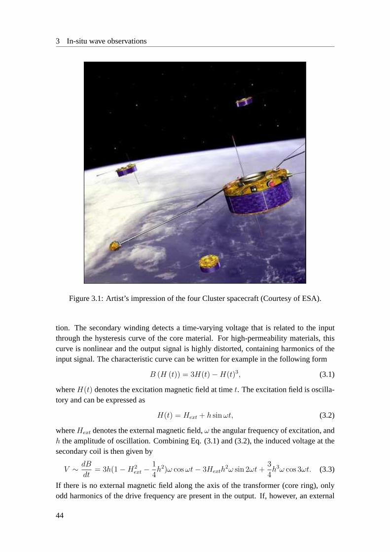
3 In-situ wave observations
Figure 3.1: Artist’s impression of the four Cluster spacecraft (Courtesy of ESA).
tion. The secondary winding detects a time-varying voltage that is related to the inputthrough the hysteresis curve of the core material. For high-permeability materials, thiscurve is nonlinear and the output signal is highly distorted, containing harmonics of theinput signal. The characteristic curve can be written for example in the following form
B (H (t)) = 3H(t)−H(t)3, (3.1)
whereH(t) denotes the excitation magnetic field at timet. The excitation field is oscilla-tory and can be expressed as
H(t) = Hext + h sinωt, (3.2)
whereHext denotes the external magnetic field,ω the angular frequency of excitation, andh the amplitude of oscillation. Combining Eq. (3.1) and (3.2), the induced voltage at thesecondary coil is then given by
V ∼ dB
dt= 3h(1−H2
ext −1
4h2)ω cosωt− 3Hexth
2ω sin 2ωt+3
4h3ω cos 3ωt. (3.3)
If there is no external magnetic field along the axis of the transformer (core ring), onlyodd harmonics of the drive frequency are present in the output. If, however, an external
44

3.2 FGM
Figure 3.2: Cluster 1 (top) and Cluster 4 (bottom) in a clean room (Courtesy of ESA).
magnetic field is present, even harmonics appear in the output. The amplitude of evenharmonics is proportional to the external field and the direction of the field along thetransformer axis. In practice, the strength of even harmonics is very weak relative tothat of odd harmonics. To amplify and detect these weak signals, the odd harmonics iseliminated by using a suitable coil geometry. In such a case only even harmonics appear inthe output. The second harmonics is amplified and detected, giving a voltage proportionalto the external field along the transformer axis.
Fig. 3.3 illustrates the electronics needed to measure one component of the mag-netic field. A precision oscillator (Oscil) generates a string of pulses at a frequency2f0,wheref0 is the final drive frequency. This signal is passed to the demodulator circuitas a reference signal, and to a frequency divider(1
2). The output of the divider (f0) is
passed through a narrow-band filter to the drive amplifier. The string of pulses from thedrive amplifier is applied to the primary (Drive) winding of the transformer. A secondarywinding around the transformer (Sense) detects the total induced signal and passes it to apreamplifier (Preamp). The output of the preamp passes through a narrow-band filter offrequency2f0 and is further amplified. A strong signal of frequency2f0 is then presentedto the synchronous demodulator. This is simply an electronic double-pole, double-throwswitch. Each time the input waveform starts to change sign, the switch is activated by thereference signal, making the output signal positive or negative depending on whether theinput lags or leads the reference by180. The output waveform thus has a frequency of2f0. The output of the demodulator is input to an integrator/amplifier that smooths overmany cycles of the rectified waveform, producing a near-dc voltage, with amplitude pro-
45

3 In-situ wave observations
Figure 3.3: Schematic illustration showing the basic components of a (single axis) flux-gate magnetometer (McPherron1995). The axis of sensitivity lies in the vertical direction,i.e. perpendicular to the sense winding.
portional to that of the second harmonics component output by the sensor, and with signdepending on the phase of the second harmonic relative to the reference signal. These twoquantities are, respectively, proportional to the magnitude and direction of the componentof the external magnetic field along the axis of the transformer. This low-frequency signalis the magnetometer output. The output voltage is also used to supply a current to an offsetwinding wrapped around the transformer. The coil constant of this winding and a feed-back resistor are chosen so that the current that flows in the offset winding will exactlycancel the magnetic field along the coil axis. Thus, the fluxgate magnetometer serves onlyas a null detector, making the entire instrument very linear over a large dynamic range.Three components of a vector field are measured by three separate sensors with their ringcore axes in mutually orthogonal directions. A fluxgate magnetometer is not an absoluteinstrument like the proton-precession magnetometer, and so it must be calibrated againststandards. Such a calibration requires large non-magnetic test facilities with three-axiscalibration coils, proton magnetometers, and optical theodolites.
FGM on each Cluster spacecraft (Balogh et al.1997, 2001) consists of two tri-axialfluxgate magnetic field sensors on one of the two radial booms of the spacecraft, and anelectronics unit on the main equipment platform (Fig. 3.4). The instrument is designedto be highly failure-tolerant through a full redundancy of all its functions. Either of thetwo magnetometer sensors can be used as the primary sensor for the main data streamfrom the instrument. In normal operations the outboard sensor located at the end of the5 m radial boom is designated as the primary source of the data. The magnetometerscan measure the three components of the field in seven ranges from 64 nT (smallest) to65536 nT (largest). The sampling of vectors from the magnetometer sensor designated asthe primary sensor is carried out at the rate of 201.793 vectors/s. This internal samplingrate has been selected to provide an appropriate set of lower rates after filtering for thedifferent telemetry modes and to give the highest frequency response for the short periodsof interest. The main operational modes of the FGM instrument provide the sampling rate
46

3.3 CIS
Figure 3.4: Fluxgate Magnetometer for the Cluster spacecraft consisting of Digital Pro-cessing Unit (DPU, left), outbound sensor with a long cable (right) and inbound sensor(middle, Courtesy of A. Balogh and E. Lucek).
from 15.52 vectors/s (normal mode) to 67.25 vectors/s (burst mode). The clock signalused for it is derived from a223 Hz (∼ 8 MHz) crystal oscillator internal to the instrument.The calibration of FGM was made in Braunschweig.
3.3 CIS
The ion data are used for the Doppler shift correction, calculation of the Alfven veloc-ity, and investigating correlations and coherences with the magnetic field fluctuations.CIS (Cluster Ion Spectrometry) measures both the cold and hot ions of Maxwellian andnon-Maxwellian populations (e.g. beams) from various plasma regimes such as the so-lar wind, the magnetosheath, the magnetosphere, and the ionosphere (Reme et al.2001).It is designed to achieve following features: (1) A uniform coverage of ions over theentire steradian solid angle with good angular resolution; (2) Separation of the major ionspecies from the solar wind to the ionosphere (H+, He++, He+ and O+); (3) High sensitiv-ity, large dynamic range, and high time resolution; (4) High angular sampling resolution(5.6 × 5.6) to detect ion beams and solar wind directions; (5) Wide range of energiesup to about 40 keV/e. The CIS instrument consists of two different instruments: HIA(Hot Ion Analyzer) sensor and CODIF (time-of-flight ion COmposition and DIstributionFunction) sensor (Fig. 3.5).
HIA measures ion energy per charge by electrostatic deflection in a symmetrical
47

3 In-situ wave observations
Figure 3.5: CODIF (on the left) and HIA (on the right) ion detectors of the CIS experiment(Courtesy of H. Reme).
quadrispherical analyzer which has a uniform angle-energy response with a fast imag-ing particle detection system (‘top hat’ model, Fig. 3.6). This particle imaging is basedon microchannel plate (MCP) electron multipliers and position encoding discrete anodes.HIA consists of three concentric spherical elements: an inner hemisphere, an outer hemi-sphere which contains a circular opening, and a small circular top cap which defines theentrance aperture. In the analyzer an electrostatic potential is applied between the innerand the outer hemisphere, allowing only charged particles with a limited range of energyand initial entrance angle to transmit. The particles are deflected by90 (quadrispherical)and detected by MCP. The particle exit position is a measure of the incident polar anglewhich can be resolved by a suitable position-sensitive detector system. A full4π steradianscan is completed every spin of the spacecraft (about 4s), giving a full 3D distribution ofions in the energy range 5 eV/e to 32 keV/e.
CODIF is a high sensitivity mass-resolving spectrometer (Fig. 3.7). It measures com-plete 3D distribution functions of the major ion species (H+, He++, He+ and O+) withinone spin period of the spacecraft. The sensor primarily covers the energy range between0.02-38 keV/charge. With an additional Retarding Potential Analyzer (RPA) device in theaperture system of the sensor with pre-acceleration for energies below 25 eV/e. CODIFcombines the ion energy per charge with a subsequent velocity measurement (time-of-flight analysis) after acceleration to≤ 15 keV/e. The energy per charge analyzer is arotationally symmetric toroidal type, which is basically similar to the quadrispheric tophat analyzer used for HIA. RPA allows to extend the energy range below 15 eV/e. Thetime-of-flight analysis measures the velocity of charged particle through the length of theunit d and the timeτ . After passing the electrostatic analyzer the ions are focused onto
48

3.3 CIS
Figure 3.6: Schematic illustration showing the basic components of the HIA sensor (Remeet al.2001).
a plane close to the entrance foil of time-of-flight (TOF) section, which is held at thepotential in order to accelerate the ions. The flight path of the ions is defined by the 3cm distance between the carbon foil at the entrance and the surface of the ‘stop’ MCP.The ‘start’ signal is provided by secondary electrons, which are emitted from the carbonfoil during the passage of the ions. The mass per charge of the ionM/Q is derived asM/Q = 2(E/Q+eUacc)(d/τ)
−2α, whereeUacc is the energy gained by acceleration afterthe electrostatic analyzer, andα is the effect of energy loss in the thin carbon foil (∼ 3 µgcm−2) at the entry of the TOF section.
Both HIA and CODIF are able to measure the velocity distribution function of ionsf(v,x, t). One can compute the velocity moments of the distribution function in orderto obtain the particle number density, bulk velocity, pressure or temperature, and heat-flux (Paschmann et al.2000). If we simply indicate withf(v) the velocity distributionfunction, we define the quantityMn, as moment of ordern of the distribution
Mn =
∫vnf(v)d3v. (3.4)
It follows that the first four velocity moments are the following:
• the number density
n =
∫f(v)d3v, (3.5)
• the number flux density vector
nV =
∫vf(v)d3v, (3.6)
49

3 In-situ wave observations
Figure 3.7: Schematic illustration showing the basic components of the CODIF sensor(Reme et al.2001).
• the momentum flux density tensor
Π = m
∫vvf(v)d3v, (3.7)
• the energy flux density vector
Q =m
2
∫v2vf(v)d3v, (3.8)
wherem denotes the ion mass.Once the zero-order moment is computed, one can obtain the bulk velocity vector
from Eq. (3.6), and computeΠ andQ in terms of velocity differences with respect to thebulk velocity. Therefore the pressure tensorP and the heat flux vectorq can be obtainedfrom Eq. (3.7) and Eq. (3.8) as:
P = m
∫(v − V )(v − V )f(v)d3v, (3.9)
and
q =m
2
∫(v − V ) · (v − V )(v − V )f(v)d3v. (3.10)
Moreover, using the relationP = nkBT one can extract the temperature tensor fromEq. (3.5) and Eq. (3.9). Finally, the scalar pressureP and temperatureT can be obtainedfrom the trace of the respective tensors:
P =TrP3
(3.11)
and
T =TrT
3. (3.12)
50

3.4 PEACE
Figure 3.8: Schematic illustration showing the basic components of the PEACE sensor(Johnstone et al.1997).
3.4 PEACE
A PEACE instrument (Plasma Electron And Current Experiment) is designed to measurethe electron velocity distribution, covering an energy range of 0.7 eV to about 30 keVand detecting electrons arriving from all possible directions (i.e.4π steradian of solidangle). Each PEACE instrument has two sensor heads, LEEA and HEEA, which aremounted on opposite sides of the spacecraft such that the instantaneous field of view ofone is the same as that seen by the other half a spacecraft rotation period later. LEEAand HEEA differ only in geometric factor (HEEA admits more electrons than LEEA inan identical plasma). The measurement principle is the same as CIS-HIA (top hat model)but an opposite sense of electrostatic potential is applied between the inner and the outerhemisphere (Fig. 3.8, 3.9, 3.10). Both sensors sample4π steradians per one spacecraftspin. Note that each sensor covers180 in the azimuthal angle seen from the symmetryaxis of the sensor, and therefore the three dimensional velocity distribution (4π steradiancoverage) is realized per spacecraft spin.
3.5 Wave analyses
Four point measurements of Cluster provide a unique possibility to determine variouscharacteristics of waves. Above all, the investigation of wave vectors serves as a power-ful means, from which one can derive not only wavelengths and propagation directionsbut also phase velocities, dispersion relations, and more. It was not until the launch ofCluster that one obtains wave vectors in three dimension in space plasma observations.The following section introduces how to determine wave properties using both single andmulti-point measurements.
51
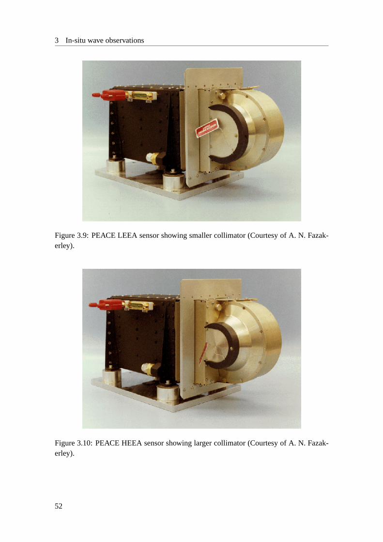
3 In-situ wave observations
Figure 3.9: PEACE LEEA sensor showing smaller collimator (Courtesy of A. N. Fazak-erley).
Figure 3.10: PEACE HEEA sensor showing larger collimator (Courtesy of A. N. Fazak-erley).
52

3.5 Wave analyses
3.5.1 Frequency and wave power
The first step to study waves is to identify frequencies of magnetic field oscillations of in-terest. It is of course possible to directly count the period of waves in the time series rep-resentation, but generally it is difficult to do because waves are not quasi-monochromaticin many cases. Instead, one computes the cross spectral density (CSD) as a function offrequency by Fourier transforming magnetic field data and identifies wave power at vari-ous frequencies to see which frequencies are contributing in the fluctuation (Jenkins andWatts1968,Bendat and Piersol1980). CSD is calculated as
C(ω, T ) =1
TB(ω)∗B(ω), (3.13)
or using the index notation,
Cij(ω, T ) =1
TBi(ω)∗Bj(ω), (3.14)
whereB(ω) denotes the Fourier component of the magnetic field fluctuation at the an-gular frequencyω for the intervalT , and the asterisk∗ denotes the complex conjugate.Subscriptsi andj run over thex, y, andz component. The diagonal component of CSD,Cii, is the wave power with respect to thei-th direction. If thez-axis is oriented to themean magnetic field direction,Cxx +Cyy andCzz yield the wave power in the transversaldirection (perpendicular to the mean field direction) and in the compressional direction(parallel to it), respectively. Trace of CSD yields the total wave power
P (ω) = TrC(ω). (3.15)
To enhance the reliability of output, the interval under investigation is often divided intosubintervals, and CSD is computed for each subinterval to average CSD. The more subin-tervals are used, the more the statistical error is reduced (Jenkins and Watts1968).
3.5.2 Ellipticity
The ellipticity evaluates how the wave field is polarized, right- or left-hand polarized, andcircularly or linearly polarized. It is determined by applying the quasi-monochromaticwave theory developed in optics (Fowler et al.1967,Arthur et al.1976,Born and Wolf1980). Provided that the magnetic field fluctuation is expressed in terms of a plane waveas
Bx(t) = a exp [i(ωt)] (3.16)
By(t) = b exp [i(ωt− π/2)] (3.17)
Bz(t) = const, (3.18)
wherea andb are the wave amplitude but can be positive or negative under the conditionthat|a| ≥ |b|, CSD at the frequencyω is calculated as
C =
a2 iab 0
−iab b2 0
0 0 0
. (3.19)
53

3 In-situ wave observations
The ellipticity ε is defined as the ratio of the minor to the major amplitude
ε =b
a= tanφ, (3.20)
whereφ may be determined from CSD as
sin 2φ =i(C21 − C12)√
(C11 − C22)2 + 4C21C12
. (3.21)
The value ofε = +1 represents the right-hand polarization, 0 for the linear polarization,and -1 for the left-hand polarization.
3.5.3 Minimum variance analysis
The divergence-free nature of magnetic fields indicates that field fluctuations are perpen-dicular to the wave propagation direction (Sonnerup and Scheible2000). The divergence-free equation is written as
∇ ·B = 0. (3.22)
When one assumes the magnetic field consisting of a constant background term and aplane wave term as
B = B0 + δB exp [i(ωt− k · x)] , (3.23)
substitution of Eq. (3.23) into Eq. (3.22) yields
k · δB = 0. (3.24)
Thus, the propagation is perpendicular to the direction of the magnetic field fluctuationwith the ambiguity of 180. This method is called theminimum variance analysis, andcan be used to determine wave propagation directions using single point magnetic fieldmeasurements.
3.5.4 Correlation and coherence
Waves exhibit in some cases a correlation or an anti-correlation between the field andthe plasma variations. For example, Alfven waves exhibit correlated magnetic field andplasma velocity fluctuations; and fast magnetosonic waves exhibit correlated magneticfield strength and plasma density fluctuations. The correlation coefficient evaluates howmuch the fluctuationx is linearly accompanied by the fluctuationy, and is defined by
r =〈(x− 〈x〉)(y − 〈y〉)〉
σxσy
=〈δxδy〉σxσy
, (3.25)
where〈 〉 denotes the expectation value, andσx andσy are the standard deviation ofxandy. The value ofr = 1 andr = −1 indicate a positive and a negative correlation,respectively. It should be noted that the linear coefficientr is defined to be the square root
54

3.5 Wave analyses
of the fraction of the variance that is explainable by the linear fit and determines part ofthe variance of the parameterx by the variance of the parametery when using a linearmodely = αx + β. This implies that(1 − r2) is the fraction of the variance ofy thatremains unexplained by the linear model. Thus, although the value ofr = 0.5 may soundlike a good fit, it means that as much as 75% of the variance is still unexplained (Reiff1983).
Coherences and phase angles can also be used to investigate the relation between thevariation ofx andy. The coherenceγ is defined as
γ =
√|Cxy|2
|Cxx||Cyy|, (3.26)
and the phase angleφ between the two fluctuations is given by
tanφ =ImCxy
ReCxy
. (3.27)
For example, the set of(γ, φ) = (1, 0) corresponds to the correlation (r = 1), and the set(γ, φ) = (1, 180) corresponds to the anti-correlation (r = −1). It is worthwhile to notethat even if the correlation coefficient is close to zero, the coherence may not be smallin general, for example in such a case that the variationx is retarded or advanced to thevariationy by the phase angle90 or 270.
3.5.5 Wave vector
The above methods can be applied to any single point measurements. However, theminimum variance analysis provides only the propagation direction with the ambiguityof 180. Furthermore, it does not derive wavelengths or propagation speeds. Gener-ally speaking, wave frequencies are modulated due to the Doppler shift in a streamingmedium, and spacecraft detect frequencies dependent on the flow speed, the spacecraftmotion, and wave vectors. In order to correct the Doppler shift, it is necessary to in-vestigate wave vectorsk. In principle, an infinite number of sensors positioned in spacewould make it possible to Fourier transform from the spatial domain to the wave numberdomain, but it is of course unrealistic. It has been found, however, that one can determinethe wave vectors from only a few measurement points in space. The method is acknowl-edged as the wave telescope (ork-filtering) technique and this enables one to calculate awave power as a function of frequency and wave vector. The wave telescope computes a3 by 3 covariance matrix
P(ω,k) = 〈b(ω,k)b†(ω,k)〉 (3.28)
of the magnetic field fluctuation amplitudeb(ω,k) at frequencyω and wave vectork,where the dagger† denotes the Hermitian conjugate. Its trace
P (ω,k) = trP(ω,k) (3.29)
55

3 In-situ wave observations
yields the spectral energy density. The task is to find the best estimator forP usingthe measured fluctuationsb(ω, rs) at the positionsrs of the spacecraft. The optimalexpression is given byPincon and Lefeuvre(1991),Motschmann et al.(1995, 1996),Glassmeier et al.(2001) as
P(ω,k) = [H†(k) M−1(ω) H(k)]−1. (3.30)
The measured magnetic field fluctuations are contained in the 12 by 12 covariance matrix
M(ω) = 〈B(ω)B†(ω)〉, (3.31)
with
B(ω) = [b(ω, r1), · · · , b(ω, r4)]T . (3.32)
The matrixH is defined as
H(k) = [Ieik·r1 , · · · , Ieik·r4 ], (3.33)
whereI denotes the 3 by 3 unit matrix. Deriving expression (3.30) requires to constructa suitable projection procedure which eliminates all signal contributions that do not cor-respond to a givenk, that is one needs to consider
P(ω,k) = W†(k) M(ω) W(k) (3.34)
with the constraint
W†(k)H(k) = I, (3.35)
whereW(k) is a weight matrix to be determined. Minimizing the trace ofP(ω,k) un-der this constraint gives the estimator (3.30) minimizing the noise. Furthermore, thedivergence-free nature of the magnetic field may be incorporated into the analysis bydemandingk ·b = 0. The effect on the minimized solution (3.30) is to replaceH(k) withH(k)V(k), yielding the optimum result
P(ω,k) = [V†(k) H†(k) M−1(ω) H(k) V(k)]−1, (3.36)
where
V(k) = I +kk
k2. (3.37)
The wave telescope assumes that waves represent superposed plane waves and thatthe the mean field has no large spatial or temporal trend. Determination of wave vectorsconsists in a search for the highest reliable wave power peaks ink-space for a givenfrequency interval. Two examples of the identified wave vectors are displayed in Fig.3.11.
56

3.5 Wave analyses
Figure 3.11: Wave power in thek-domain derived by the wave telescope technique usingCluster FGM data. The left and right panel show the presence of the anti-parallel and theperpendicular wave vector, respectively (Narita et al.2004, 2006a).
3.5.6 Frequency and phase velocity in the plasma rest frame
Once the wave vector is determined, one can correct the Doppler shift and calculate thefrequency in the plasma rest frame using the following relation
ωrest = ωsc − k · V flow, (3.38)
whereωrest andωsc denote the angular frequency in the plasma rest frame and in thespacecraft frame, respectively,k the wave vector, andV flow the plasma flow velocityvector. The spacecraft motion is neglected in this thesis, for it is of the order of a fewkm/s, whereas the flow speed in the solar wind and in the magnetosheath is about 400km/s and 100-200 km/s, respectively. The phase velocity in the plasma rest frame can befurther derived as
V ph =ω
|k|2k. (3.39)
3.5.7 Dispersion relation and propagation pattern
The wave telescope technique provides not only a method to determine the wave vectorsbut also a variety of analysis tools to identify wave modes and their propagation patterns.The relation between frequencies and wave numbers is called the dispersion relation.From a theoretical point of view, deriving dispersion relations is one of major tasks, sinceit is uniquely characterized by the distinctive wave mode. Therefore the wave mode can beunambiguously identified if the dispersion relation is properly derived from observations.The dispersion relation can be determined by applying the wave telescope technique andidentifying wave vectors at various frequencies.
Another application of the wave telescope is the wave propagation pattern in themedium. When one investigates many examples of wave events in various locations,
57

3 In-situ wave observations
one can determine a distribution of phase velocity vectors or wave vectors in the spatialcoordinate, which is a propagation pattern on the statistical basis.
58

4 Dispersion analysis of upstreamwaves
4.1 Introduction
In this chapter we use the wave telescope technique extensively and aim to derive disper-sion relations for the upstream (foreshock) waves. Furthermore, we combine the disper-sion curves with polarization properties derived from the minimum variance analysis.
The dispersion analysis was initiated by the ISEE double spacecraft mission.Hoppe etal. (1981) andHoppe and Russell(1983) estimated wave vectors for the quasi-monochro-matic wave packets in the foreshock region, investigating phase differences of the mag-netic field fluctuations at the two spacecraft. Also using the magnetic field data obtainedby the AMPTE double spacecraft in the same region,Dudok de Wit et al.(1995) andBa-likhin et al. (1997a,b) combined the minimum variance analysis with the projected wavenumbers and derived approximate dispersion relations.
The data used in the dispersion analysis in this chapter are the magnetic field datafrom Cluster FGM. The ion data from CIS-HIA are also used to obtain the mean plasmaflow velocity Vsw, the mean mass densityρ, and the ion velocity distribution. We havechosen the time interval on February 20, 2002, 1700-1730 UT for the present case. Mea-surements of spacecraft Cluster 3 are shown in Fig. 4.1. The mean magnetic field isB0 = (8.4,−3.7, 5.3) nT in the GSE coordinate system.
4.2 Dispersion analysis
The wave telescope determines both wave number vectors and their associated wavepower (Pincon and Lefeuvre1991, Motschmann et al.1995, 1996,Glassmeier et al.2001). We apply the wave telescope at various frequencies up to 11 Hz, which is theNyquist frequency of the magnetic field data used and derive experimentally dispersionrelations in three components of wave number vector. Figure 4.2 exhibits the dispersionrelations obtained in the spacecraft (s/c) frame of reference. The angular frequencyω
is normalized to the proton cyclotron frequencyΩcp = 1.1 rad Hz and the wave numbervectork is normalized to the ion inertial wave number(VA/Ωcp)
−1 = 10.3× 10⁻³ km−1,whereVA stands for the Alfven velocityB/
√µ0ρ = 108 km/s. For thekx component, a
59

4 Dispersion analysis of upstream waves
Figure 4.1: Measurements of low frequency waves in the foreshock recorded by Cluster3 in the interval on February 20, 2002, 1700-1730 UT. Magnetic field, plasma density,velocities, and temperature are displayed in the GSE coordinate system. The CIS data areaveraged on 12 seconds (Narita et al.2003).
linear dispersion branch with negative phase velocity is detected as well as another minorbranch at lower frequencies below 1 Hz. For theky component almost zero wave numbersare detected. For thekz component a linear dispersion branch at lower frequencies below2 Hz is smoothly connected to a curved branch at higher frequencies.
In the s/c frame, the mean phase velocity is estimated asV ph(sc) = ωsck/|k|2 =
(−257, 0,−58) km/s. With the background flow velocityV sw = (−402, 83,−17) km/s,one obtains the mean phase velocity in the plasma rest frameV ph(re) = V ph(sc)−V sw =
(145,−83,−75) km/s. The minus sign in front ofV sw compensates the background flowvelocity, andVph(re),x has an opposite sign with respect toVph(sc),x. Therefore,|V sw| islarger than|V ph(re)| and the spacecraft observe waves propagating in the same direction asthe background flow (anomalous Doppler shift). The Doppler shift is corrected at variousfrequencies using the relationωrest = ωsc−k·V sw, whereωrest, ωsc, andk are the angularfrequency in the plasma rest frame and in the s/c frame, and the wave number vector,respectively. Without loss of generality we change signs ofω andk asω → −ω and
60

4.2 Dispersion analysis
Figure 4.2: Dispersion relations from the wave telescope using Cluster data. Angularfrequencyω is normalized to proton cyclotron frequencyΩcp = 1.1 rad Hz and wavenumberk is normalized to ((VA/Ωcp)
−1 = 10.3×10⁻³ km−1, whereVA is Alfv en velocityB/√µ0ρ = 108 km/s. The GSE system is used for the wave number. Panels in top row
show the dispersion relations in the s/c frame and bottom panels show the one in theplasma rest frame (Narita et al.2003).
k → −k, projecting the dispersion curves into the upper right quadrant. This preserveswave phase velocity but changes representation of wave polarization properties such asthe sense of rotation of polarization from a right-handed to a left-handed representation.The resulting dispersion relation is also displayed in Fig. 4.2.
After the Doppler shift correction frequencies are diminished. Some of data points inthe dispersion relation are located in the negativeω regime in the rest frame, i.e. wavespropagating in both directions. The linear dispersion branch forkx has been changed to aslightly curved branch. The minor deviating branch at lower frequencies forkx has falleninto the negativeω regime, showing an almost straight line. Theky dispersion remainsalmost unchanged, for the Doppler shift is small. The curved branch at higher frequenciesfor kz has been broadened in the rest frame. Although signs of wave numbers have beenchanged,kx is kept predominant among the three components and the dispersion relationfor |k| exhibits the almost same curves as thekx one.
We investigate, furthermore, the sense of rotation (the sign of ellipticity in the po-larization plane) about the propagation direction using the minimum variance analysis(Fowler et al.1967). This allows one to decompose the dispersion relation into differ-ent polarization regimes. Fig. 4.3a shows a dispersion relation derived from the wavetelescope in the rest frame plotted together with the sense of rotation at various frequen-cies. Right- and left-handed polarization are represented by diamonds and plus signs,respectively. A small plot embedded in Fig. 4.3a is an enlarged plot of the dispersion
61

4 Dispersion analysis of upstream waves
Figure 4.3: Dispersion relations in the plasma rest frame derived from different sources:dispersion from the wave telescope and polarization from the minimum variance analysisfor (a) and computation using a multi-fluid plasma model for (b). Wave numberk isprojected onto a mean propagation directionθkB = 24. Angular frequencyω and wavenumberk are normalized as in Fig. 4.2 (Narita et al.2003).
relation ranged from 0.2 to 0.4 forωrest/Ωcp and from 0.0 to 0.3 forkVA/Ωcp. Wavenumberk in Fig. 4.3a is a projected onto a mean propagation directionθkB = 24, whereθkB is changed from156 to 24 to agree with the change of sign ofk in the rest frame(see above). Both right- and left-handed polarizations are found in the major and minorbranch.
To conclude, the direction of the wave propagation is dependent on frames of refer-ence. Waves propagating in the sunward direction in the rest frame are convected in theopposite direction because of the large plasma flow velocity. From the dispersion analysistwo different branches are found in the dispersion relation. A major branch shows a lineardispersion in the s/c frame but it is changed into a slightly curved branch in the rest frame.A minor branch intersecting almost perpendicularly to the major branch at lower frequen-cies in the s/c frame turns out to be an almost linear dispersion branch in the negativeω
in the rest frame. Relevant angles of the wave propagations and the background magneticfield direction are as follows. Propagation angle in the s/c frame and in the rest frame withrespect to the Earth-to-Sun direction (GSE-X) are167 and38, respectively. The IMF
62

4.3 Dispersion in a beam plasma
cone angle and the IMF spiral angle in the XY plane are38 and24, respectively.
4.3 Dispersion in a beam plasma
It is shown that a beam plasma system explains the dispersion relation of the low fre-quency waves in the foreshock. We assume a beam plasma system composed of twodifferent species: a cold plasma component and a beam with lower density and highervelocity. In a cold plasma treatment there appear four branches in the dispersion rela-tion for transverse low frequency waves for propagation quasi-parallel to the magneticfield, that is right- and left-handed polarization, propagating both forward and backwardto the magnetic field. When the ion beam is present a resonant wave emerges due tothe ion beam instability. The resonant wave satisfies the cyclotron resonance conditionωrest− kvb + Ωb = 0, wherevb andΩb are the velocity and the cyclotron frequency of thebeam, respectively.
Assuming the following parameters (justified later) for multi-fluid plasma model givesone a theoretical dispersion relation displayed in Fig. 4.3b: 0.001 (i.e. 0.1%) for the ratioof the beam density to the cold plasma density; 5.6 for the Alfven Mach number of thebeam; and quasi-parallel propagation (θkB = 24). The wave propagation angleθkB
has been chosen to be the same as the mean propagation angle from the wave telescopeinvestigation.
In Fig. 4.3b there are five branches in the dispersion relation. The linear dispersionbranchRes.in Fig. 4.3b stands for a resonant wave of the beam. Other branches originatefrom the cold plasma:R+, L+, L− , R− in Fig. 4.3b, where ‘+’ stands for a forwardpropagation to magnetic field and ‘−’ for a backward propagation, andR for right-handedpolarization andL for left-handed polarization.
The dispersion relation Fig. 4.3a is identified as a part of Fig. 4.3b for the followingreasons. First, a major curved branch with frequencies up to 3 Hz in Fig. 4.3a correspondsto theR+ branch in Fig. 4.3b, although the curvature of the branch is slightly different.Second, the linear part in the negativeω in Fig. 4.3a is identified as the linear resonantbranch in Fig. 4.3b. When the beam density is smaller enough than the backgroundplasma density, this branch is given byω− kvb + Ωb = 0. Identification of the linear partof the branch in the experimentally derived dispersion relation allows one to determinevb and Ωb. The beam velocity is estimated asvb = 604 km/s in the rest frame, thatis 5.6 for the Alfven Mach number. The beam species are identified as protons, sinceωrest/Ωcp ' −1 atk = 0 in Fig. 4.3a. These values justify the initial parameters used forthe calculation of the dispersion relation in Fig. 4.3b.
Figure 4.4 is the ion distribution function obtained from the CIS-HIA measurements,exhibiting two gyrating ion populations (reflected ions) around(V⊥, V‖) = (−482, 79)
km/s and(579, 107) km/s and solar wind ions around(232,−339) km/s. The mean dif-ference inV‖ between the gyrating ions and the solar wind ions is 432 km/s. This valuedoes not deviate fromvb derived from the dispersion analysis. The gyrating ions associ-
63

4 Dispersion analysis of upstream waves
Figure 4.4: Ion distribution function in the velocity space (V⊥ andV‖) measured by CIS-HIA in unit of fdist [s3/km6]. V⊥ is along the projection of bulk velocity onto the planeperpendicular to magnetic field (Narita et al.2003).
ated with the foreshock waves have been reported inMeziane et al.(2001). These ionsmay be considered as ions which form a beam at first and obtain energy in the perpendic-ular direction through the instability.
Our scenario for the foreshock waves is that a fraction of the upstream proton popula-tion is reflected at the shock forming a beam and subsequently generating low frequencywaves by means of the ion beam instability. This is in good agreement with one of thephysical processes in the foreshock suggested by a number of observations and theoreticalworks on the right-hand ion beam instability.
4.4 Discussion
The wave telescope has been used extensively to study the dispersion relation of the lowfrequency waves in the foreshock for quasi-parallel propagation. The dispersion analysisindicates the presence of a backstreaming proton population reflected at the shock and theion distribution function shows gyrating ions which can be considered as beam protonsafter the occurrence of the beam instability.
From the dispersion analysis it is also found that the Doppler shift plays an importantrole in studying wave frequencies and propagation directions. The propagation direction
64

4.5 Summary
is reversed when the Doppler shift exceeds wave frequencies in the rest frame. From acomparison of the dispersion relations it is likely that a beam plasma system explains notonly properties of the foreshock waves but also their physical process of wave generation.Although further quantitative investigations, as well as more event studies, are needed tojustify our result, backstreaming ions are probably responsible for the generation mecha-nism of low frequency waves in the foreshock.
We have seen that our result in Fig. 4.3a derived from the wave telescope may beexplained by a beam plasma system. Several difficulties, however, need to be solvedboth qualitatively and quantitatively. First, frequency for the cyclotron resonance andcurvature, or group velocity, of theR+ branch is slightly different. Second, not onlyright-handed but also left-handed polarization are found in the major branch Fig. 4.3a.In theory, dispersion relations are separated into different polarizations. The sign of el-lipticity in the polarization plane obtained from the minimum variance analysis has beenadopted to investigate the sense of rotation, but this analysis is subject to noise when de-termining the polarization plane. Different method will be tested to examine polarizationsmore, e.g. Stokes parameter method. Third, information on the beam density is not de-rived from the dispersion relation, because the condition for the cyclotron resonance doesnot contain the density parameter. The density of the reflected ions from CIS-HIA will beestimated and used to improve the quality of the numerical dispersion relation.
4.5 Summary
We have analyzed low frequency wave activity in the near-Earth shock upstream solarwind. Using Cluster as a wave telescope we have investigated in detail wave propagationdirections and wave numbers for various frequencies, obtaining, for the first time, threedimensional dispersion relations experimentally. After Doppler shift correction, we findthat the dispersion relations are not linear and the waves are propagating in the sunwarddirection in the plasma rest frame. Comparison of the experimentally derived dispersionrelation with that one for a beam plasma system shows good agreement. The results sug-gest that the waves in the foreshock are generated by the proton population backstreamingfrom the shock.
65

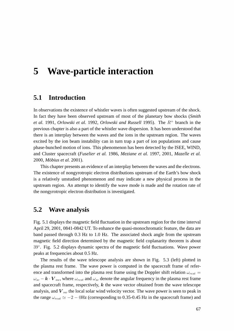
5 Wave-particle interaction
5.1 Introduction
In observations the existence of whistler waves is often suggested upstream of the shock.In fact they have been observed upstream of most of the planetary bow shocks (Smithet al. 1991,Orlowski et al.1992,Orlowski and Russell1995). TheR+ branch in theprevious chapter is also a part of the whistler wave dispersion. It has been understood thatthere is an interplay between the waves and the ions in the upstream region. The wavesexcited by the ion beam instability can in turn trap a part of ion populations and causephase-bunched motion of ions. This phenomenon has been detected by the ISEE, WIND,and Cluster spacecraft (Fuselier et al.1986,Meziane et al.1997, 2001,Mazelle et al.2000,Mobius et al.2001).
This chapter presents an evidence of an interplay between the waves and the electrons.The existence of nongyrotropic electron distributions upstream of the Earth’s bow shockis a relatively unstudied phenomenon and may indicate a new physical process in theupstream region. An attempt to identify the wave mode is made and the rotation rate ofthe nongyrotropic electron distribution is investigated.
5.2 Wave analysis
Fig. 5.1 displays the magnetic field fluctuation in the upstream region for the time intervalApril 29, 2001, 0841-0842 UT. To enhance the quasi-monochromatic feature, the data areband passed through 0.3 Hz to 1.0 Hz. The associated shock angle from the upstreammagnetic field direction determined by the magnetic field coplanarity theorem is about39. Fig. 5.2 displays dynamic spectra of the magnetic field fluctuations. Wave powerpeaks at frequencies about 0.5 Hz.
The results of the wave telescope analysis are shown in Fig. 5.3 (left) plotted inthe plasma rest frame. The wave power is computed in the spacecraft frame of refer-ence and transformed into the plasma rest frame using the Doppler shift relationωrest =
ωsc − k ·V sw, whereωrest andωsc denote the angular frequency in the plasma rest frameand spacecraft frame, respectively,k the wave vector obtained from the wave telescopeanalysis, andV sw the local solar wind velocity vector. The wave power is seen to peak inthe rangeωrest ' −2− 0Hz (corresponding to 0.35-0.45 Hz in the spacecraft frame) and
67

5 Wave-particle interaction in the upstream region
Figure 5.1: Magnetic field input to the wave telescope analysis from Cluster 4. Thedata have been passed through a 0.3 - 1.0 Hz band pass filter and had the backgroundmagnetic field subtracted. (Bottom) Dynamic wave power spectrograms for the magneticfield components and total field observed on Cluster 4. Black vertical lines denote thetime period of the event. Power has units of nT2/Hz (Gurgiolo et al.2005).The spacecraftis in an outbound orbit and positioned at [8.7, -7.8, 8.8]RE in the GSE coordinate system.The spacecraft moves 100 km outbound within the displayed interval.
k ' 4−6×10⁻³ km−1. The wave is propagating anti-sunward in the spacecraft frame butwith the Doppler shift correction it is propagating sunward, as the dominant frequenciesare negative in the plasma rest frame.
Fig. 5.3 (right) replots the data in Fig. 5.3 (left) over the restricted frequency range-4 to 4 Hz. In addition the sign of the frequency has been reversed to locate the maindispersion curve in the upper half plane. Changing the sign of the frequency transformsthe propagation direction asθkB → 180 − θkB, which is seen in the lower plot. Overlaidon the upper plot in white is the dispersion curve of the ordinary right-hand whistlerwave (cold plasma limit, electrons and ions included,30 propagation) computed usingthe observed local field and plasma conditions: B = 10.1 nT and n = 11.8 cm−3. The
68

5.2 Wave analysis
Figure 5.2: Dynamic wave power spectrograms for the magnetic field components andtotal field observed on Cluster 4. Black vertical lines denote the time period of the event.Power has units of nT2/Hz (Gurgiolo et al.2005).
dispersion relation was determined by the Appleton-Hartree equation
N2 =B ±
√B2 − 4AC
2A, (5.1)
which is the equation for the wave refraction index
N =ck
ω, (5.2)
wherec denotes the speed of light,k the wave number, andω the wave angular frequency.The coefficients of the equation can be determined by applying the cold plasma model,and they are functions of the background plasma density and magnetic field, the wavefrequency, and the propagation direction (Baumjohann and Treumann1997). The qual-itative fit of the theoretical to the derived dispersion curves is a good indication that thewaves responsible for the phase trapping are the right-hand whistlers. The derived disper-sion relation, however, tends to have larger frequencies and phase speeds than indicatedin the theoretical branch shown. This probably implies that not all of the measured elec-trons and ions contribute to the waves (as assumed in the cold plasma theory). A lowereffective density increases the local Alfven speed. (The whistler wave phase speed at lowfrequencies approaches the Alfven speed.) The argument for a lower density is based onthe inclusion of the halo electron population in the measured density.
Hodograms of the magnetic field fluctuation in the spacecraft frame of reference showthat the wave is left-hand circularly polarized about the magnetic field direction (Fig. 5.4).The waves are right-hand circularly polarized in the plasma rest frame.
69

5 Wave-particle interaction in the upstream region
Figure 5.3: (Left) Results of the wave telescope analysis on the 0.3 to 1.0 Hz band passedmagnetic field data. Upper plot is the wave power as a function of the angular frequencyand wave number in the plasma rest frame. The lower plot shows the wave propagationangle with respect to the background magnetic field; (Right) Comparison of the ordinaryright-hand whistler wave dispersion curve (dashed line) generated using the local mag-netic field and plasma parameters with the dispersion pattern arrived through the wavetelescope analysis of the local magnetic field data (Gurgiolo et al.2005).
5.3 Phase-bunched electrons
Fig. 5.5 displays a matrix of plots, each of which contains data from the 178.5 eV-centeredPEACE sweep step taken over one satellite spin. Plots within a column come from onesatellite (see label at the top of each column) and within a row from the same spin (asclose as can be matched in time between the three satellites). The plots themselves areequidistant cylindrical projections of the velocity space shell containing the measureddata. The coordinates are GSE with polar angle plotted along Y and azimuthal angleplotted along X. A90 polar angle points to within2 − 6 of -Z GSE and0 in azimuthpoints toward the sun. The measured particle velocity is opposite to these directions sothat particles observed at positive polar angles are moving toward the +Z hemisphere anda particle observed at0 azimuth angle is traveling anti-sunward. All plots are in the localplasma rest frame.
The plots show two distinct particle populations: A compact oval of particles at pos-itive polar angles that are high-energy solar wind halo electrons moving anti-sunwardand a more spread out population centered near180 moving back upstream. The whiteplus signs within both the halo and return populations are mappings of the head and tailof every magnetic field vector measured during the observations. Their spread indicates
70

5.3 Phase-bunched electrons
Figure 5.4: Hodogram of the magnetic field at Cluster 4 during the observations of thenongyrotropic electrons.δB⊥1 is aligned with the Earth-Sun line and projected onto theplane perpendicular to the magnetic field (Gurgiolo et al.2005).
Figure 5.5: Phase-elevation plots of the 178.5 eV channel from Cluster 1, 2, and 3 showingthe rotation of the nongyrotropic component of the electron distribution in Cluster 3 and 4.Red arrows in the middle plot in the last column indicate the halo (H) and back-streaming(BS) electron populations (Gurgiolo et al.2005).
changes in direction of the magnetic field during the measurement. The instrument islooking parallel to the magnetic field when observing the halo electrons. Any apparentoffset of the halo electron population from the magnetic field can be attributed to the factthat the instrument measurement bins may not be centered on the magnetic field. Such
71

5 Wave-particle interaction in the upstream region
cannot be claimed for the nongyrotropic signatures in the back-streaming electrons whichare more than a measurement bin width off the field.
At both Cluster 3 and 4 the return electrons exhibit a clear nongyrotropic signatureseen as an intensification at various phases with respect to the magnetic field. Cluster1 also shows a nongyrotropic signature in the backward streaming electrons but only inthe last plot. What is striking about the plots from both Cluster 3 and 4 is the apparentrotation of the nongyrotropic signature in the return beam from spin to spin. As willbe shown later, the rotation is real but somewhat deceiving since it cannot be measureddirectly from the plots.
It is important to understand how the PEACE instrument samples the data in order tounderstand and interpret what is seen in Fig. 5.5. Fig. 5.6 displays a basic measurementpattern for a single energy step used by the PEACE instrument through one spin of data.There are 384 measurements taken within each spin, one from each of the 12 elevationzones in each of the 32 sectors. The measurements for all of the elevations are taken si-multaneously (shaded bar). They occur in a time TM followed by a dead-time TD. Thedead-time represents the time expended on the measurements of the other energy stepsthat make up the full energy sweep. During the measurement cycle the nongyrotropicportion of the distribution is rotating about the local magnetic field. This sets up a beatingpattern between the distribution and the measurement cycle. Counts are registered when-ever a portion of the distribution overlaps grids in which measurements are being made.The beating of the distribution function with the measurement cycle has two immediateconsequences. First, it allows a nongyrotropic distribution to retain a nongyrotropic sig-nature up to the point where the distribution makes one or more rotations within a singlemeasurement time (TM). At that point the distribution will appear in every measurementbin that it overlaps. The data used in this paper has a measurement time of about 0.0039 swhich gives a minimum rotation rate of 256 Hz before the data would appear as a ring inplots of Fig. 5.5. In actuality, this rate will be slightly smaller due to the thermal extent ofthe distribution. The second consequence is that when the distribution has a rotation thatallows it to move over multiple phase sectors during a measurement time TM, the distri-bution will generally be oversampled within a spin. The result of this is that the particlesmay be seen in multiple measurement bins. So while it may be possible to determine if adistribution has a nongyrotropic component, it is often not possible to say anything aboutits morphology.
An estimation of the rotation period of the nongyrotropic components of the distri-butions seen in Fig. 5.5 in both Cluster 3 and 4 can be made on the assumption that therotation period has no time dependency over the 12 s of data shown. In this case themeasured rotation phase should follow the linear relationship
P + 360 ·N(T ) = Ω · T + P0, (5.3)
whereP is the measured rotation phase at timeT , P + 360 ·N is the number of degreesthrough which the distribution has rotated sinceT = 0, N is an integer,Ω is the rota-tion rate in degrees/second, andP0 is the distribution phase atT = 0. The360 · N term
72

5.3 Phase-bunched electrons
Figure 5.6: The Plasma Electron and Current Experiment (PEACE) measurement matrixfor a single energy step. Grids within a column represent the elevation sensors and withina row the azimuthal sectors. Measurements in a column are simultaneous and in a row aresequential. (Gurgiolo et al.2005)
is required because the distribution may have rotated multiple times between measure-ments. Note that the term is not a constant in the equation but depends on the time of themeasurement.
The approach to solving Eq. (5.3) is to varyN to minimize the standard deviationin the least squares fit. The result of this minimization is shown in Fig. 5.7 for thedistributions seen in both Cluster 3 and 4 in Fig. 5.5. In the plot,x represents data takenfrom main nongyrotropic signature in Cluster 3 ando represents data taken from Cluster4. T = 0 is the time of the observation of the nongyrotropic component in the first plotin Cluster 3. All other times are measured relative to this time. Both sets of data showa good fit by the linear relationship in Eq. (5.3) with rotation rates ofΩ = −180/s(i.e. f = −0.5 Hz) for Cluster 3 andΩ = −175/s (−0.486 Hz) for Cluster 4, which areclose to the frequencies seen in the waves observed in the magnetic field data (Fig. 5.2).Negative rotation rates correspond to left-hand rotations in the way the problem is set up.
Two additional sets of data are also shown in Fig. 5.7. In the Cluster 3 plots, there is inaddition to the primary nongyrotropic signature, a weaker signature that is also rotating.The weaker signature can be seen diagonally opposite to the primary signature and prob-ably results from secondary samplings of the distribution in its gyration. The phase-timerelationships for the features were determined identically to that for the primary signa-ture and were added to Fig. 5.7 as number symbols (#). With the exception of the lastobservation, they map very well to the established linear rotation-time relationship.
The second set of data added to the plot is represented by the plus symbols. These
73

5 Wave-particle interaction in the upstream region
Figure 5.7: The relationship of the nongyrotropic phase angle with time.T = 0 is thetime of the first observation of the nongyrotropic component in Cluster 3 in Fig. 5.5. Thefit coefficients for each line are given at the top of the plot with their computed variancesin the parenthesis (Gurgiolo et al.2005).
are the Cluster 4 data (circles) offset in phase by180. This shifts the Cluster 4 data tomap onto the Cluster 3 data. If the premise that the observed nongyrotropic signatures arephase locked by the locally observed waves is correct, then the separation of the two linesshould represent a phase shift in the phases of the waves observed at Cluster 3 and 4.
5.4 Discussion
Fig. 5.7 exhibits that the nongyrotropic portion of the distribution is not rotating at theelectron Larmor frequency (≈ 320 Hz for the local field strength) but is rotating verynearly at the local wave frequency, probably within measurements errors. The largesterrors in the computation of the rotation frequency come in the estimation of the rotationphase angle and the assumption that the rotation frequency is a constant over the timeperiod.
Errors in the estimation of the phase of the nongyrotropic distribution are due basi-cally to the finite bin size over which the measurements are taken. The error in phasesector can almost be ignored. The actual measurement occurs within a time interval equalto 1/32 of total sector time. The error introduced by the elevation angle bin is more sig-
74

5.5 Summary
nificant. While PEACE takes measurements in 12 elevation bins, these are often summedfor telemetry reasons. At the time of the measurements presented here, PEACE was re-turning data at only six elevation angles (sums of the adjacent even and odd numberedpolar zones). The large bin sizes do not, however, translate into equally large errors inthe rotation phase. The narrow range in spin phase restricts the error in the arc tangentwhen computing the distribution phase and the understanding that the distribution is ro-tating about a definite circular path centered on the magnetic field (which can generallyeasily be estimated from the elevation-phase plots) allows an estimation of the elevationangle within a bin. Even an error in the determined phase as large as±30 results inonly a±0.05 Hz error in the rotation frequency. The small error is due to the fact thatthe distribution has rotated through a much larger angle than is measured from the plotsalone.
There are two additional errors that may come into play. The first arises from theassumption that the rotation rate is constant over the three spins during which the mea-surements are taken. Small changes in the frequency of the peak power shown in Fig. 5.2,especially near the end of the time period, suggest that this probably is not true, whichcould explain why the last observation of the secondary nongyrotropic feature falls so faroff the nominal rotation-time relationship. The overall linearity of the data in Fig. 5.7,however, suggests that the variations in rotation rate are probably not large. The secondsource of error is a result of the motion of the center of mass of the distribution due tochanges in the magnetic field direction during the measurement time frame. This errorcannot be larger than the spread in the plus symbols in Fig. 5.5 and in general is muchsmaller, since the nongyrotropic signature occurs only over a small portion of the timeduring which the backstreaming electrons are observed.
5.5 Summary
The close correlation of the observed rotation frequency of the nongyrotropic electrondistribution upstream of the Earth s bow shock with the frequency corresponding to themaximum in the spectral power density in the local waves in the magnetic field suggestsa relationship between the two. This is strengthened by the ability to overlay the obser-vations made at Cluster 3 and 4 simply by using the observed phase shift in the magneticwaves between the two satellites.
At this time it is impossible to say whether the magnetic field fluctuations are respon-sible for the formation of the nongyrotropic signature or if the nongyrotropic electrons arethe source of the instability that produces the waves. In either scenario the magnetic wavesact as a shepherd wave for the nongyrotropic electrons preventing them from gyrophasemixing as they move upstream of the bow shock.
Using a wave telescope analysis on the magnetic field, the waves are shown to mostprobably be ordinary right-hand whistler waves. Whistler waves are commonly observedupstream of the Earth s shock. The association of whistler waves and nongyrotropic elec-
75

5 Wave-particle interaction in the upstream region
trons may indicate that nongyrotropic electron distribution are more prevalent in the Earths foreshock than might be thought. While there are a number of studies which address theformation of the whistlers within the foreshock region both through instability analysisand simulations, none consider the effects of the waves on the background electrons. Theresults suggest this be undertaken. When these types of studies are completed, not onlywill we have a better idea of the role of the whistler wave in the formation of nongy-rotropic electrons but also what if any role these distributions have in the electron physicstaking place upstream of the shock.
76

6 Statistical study of upstream waves
6.1 Introduction
In the previous chapters the wave mode identification through the dispersion analysis isthe goal of the study. Investigating wave vectors is a powerful means in wave analyses.It provides phase speeds and their directions, and also brings a possibility to answer thequestion of how they propagate, namely what their propagation pattern looks like. Thepropagation pattern in the bow shock environment has not been derived on a statisticalbasis so far. Yet, the early spacecraft already derived that the propagation sense of the up-stream waves is toward upstream (away from the shock) in the plasma rest frame in somecase studies (Hoppe et al.1981,Hoppe and Russell1983), which is further confirmed inChapter 4, 5 and also byEastwood et al.(2002).
This chapter presents a statistical study of the upstream waves. The waves are stud-ied in the plasma rest frame using Cluster data. Magnetic field data of 1 and 4 secondsresolution from FGM are used and the wave telescope is applied to obtain the wave num-ber vectors. Ion density and velocity data from CIS-HIA from Cluster 3 are also used tocalculate the Alfven velocities and the Doppler shifts.
6.2 Case study
Fig. 6.1 displays the magnitude of magnetic field, the ion density, and the ion bulk velocityin time domain measured by Cluster 3 from 0400 to 1000 UT on February 18, 2002. Theforeshock wave in this event exhibits the clearest example in wave power spectra andtypical features which will be drawn in the statistical study. The spacecraft separation isas small as 100 km and the time series plots of magnetic field display almost the sameresults among different spacecraft. Cluster observes the dayside northern magnetosphere(0400 - 0500 UT), the magnetosheath (0500 - 0800), and the upstream solar wind region(0800 - 1000) with several shock crossings. The angle between the upstream magneticfield and the shock normal determined from the method of coplanarity theorem is 2.6
for the Cluster 3 observation. In the upstream region a moderately active fluctuation ofthe magnetic field is observed between 0800 and 0900 UT with the average summed
77

6 Statistical study of upstream waves
Figure 6.1: Measurements of the magnitude of magnetic field from FGM, ion density andbulk velocity from CIS-HIA made by Cluster 3 from 0400 to 1000 UT on Feb. 18, 2002.‘FS’ between 0805 and 0840 UT stands for an interval of the foreshock wave observation(Narita et al.2004).
component of normalized magnetic field deviation (for 4 seconds data)
〈σ2〉 = 〈|∆Bx|2 + |∆By|2 + |∆Bz|2
|B|2〉 ∼ 0.365, (6.1)
whereas the fluctuation is quiet after 0900 UT. We take the interval 0805 - 0840 UTfor the case study of the foreshock waves. The mean value of interplanetary magneticfield (IMF) is B = (8.4, -4.1, 2.5) nT in GSE and the IMF cone angle (angle betweenthe magnetic field direction and thex-axis) is 29.8. Our analysis method is as follows.First, the geometrical configuration of the foreshock observation is investigated. Then thedominant frequency in the spacecraft frame is identified from the power spectrum and thewave number is identified using the wave telescope. The Doppler shift is corrected toderive the rest frame frequency and the phase velocity. The ellipticity of polarization isalso investigated using quasi-monochromatic wave theory.
The foreshock is generally connected to the shock by the magnetic field. We inves-tigate the geometrical configuration for Cluster 3 which provides us with both the FGMand the CIS-HIA data and ask whether the observation is made in the foreshock regionor not. We assume that the CIS-HIA data from Cluster 3 are valid for other spacecraft inwave analysis later. For simplicity we adopt an empirical, parabolic bow shock model
X = as − bs(Y2 + Z2), (6.2)
78

6.2 Case study
whereas is the bow shock standoff distance in unit ofRE from the Earth andbs is theflaring parameter in unit ofR−1
E (Merka et al.2003). The bow shock is well represented bya paraboloid for GSE-X larger than -40RE (Cairns et al.1995). The coordinate system isaberrated so that the direction ofx-axis is opposite to the solar wind velocityV sw and thexy plane is made byV sw and IMF orientation (we call thexy plane VB plane). The IMFanglearctan(By/Bx) in the VB plane is 47.6. The solar wind dynamic pressure and thefast magnetosonic Mach number calculated from Cluster 3 data are applied to obtainas
andbs using the relations
as = amp
[1 + 1.1
(γ − 1)M2 + 2
(γ + 1)(M2 − 1)
](6.3)
bs = 0.0223(Psw
1.8)
16 R−1
E , (6.4)
whereamp is the magnetopause standoff distance,γ is the effective ratio of specific heatsand assumed to be5/3, M is the fast magnetosonic Mach number (Russell1985),Psw isthe solar wind dynamic pressure in unit of nPa. Equation (6.3) and (6.4) were proposedby Farris and Russell(1994) andCairns et al.(1995), respectively.amp is calculatedfor the magnetopause model ofShue et al.(1997). We obtainas = 14.0RE andbs =
2.25× 10⁻²R−1E . Now consider the equation
r = r0 +DeB (6.5)
which relates the intersection of the IMF line connected to the spacecraft at the shockr
to the spacecraft positionr0 = (x0, y0, z0) and the distance between themD (See Fig.6.2).eB = (ex, ey, ez) is a unit vector of IMF and it is assumed that there is no change inmagnetic field topology.D may take negative values, depending on the direction of IMFand the spacecraft position. Combining equation (6.2) with (6.5), one obtains a quadraticequation forD
bs(e2y + e2z)D
2 + [ex + 2bs(y0ey + z0ez)]D + [x0 − as + bs(y0ey + z0ez)] = 0. (6.6)
Real solutions forD represent the spacecraft located in the foreshock region. We obtainD = −14.1RE. The distance between tangential magnetic field line to the shock and thespacecraft alongV sw is 5.2RE. Fig. 6.2 displays a sketch of the result in the VB planetranslated inz direction to the spacecraft position atzV B = −26RE.
Fig. 6.3 displays the power spectrum of the magnetic field fluctuation derived fromthe Fast Fourier Transform (FFT) for Cluster 3. A peak in power is identified at frequency44.9 mHz (period of 22 seconds). Power spectra derived from the other Cluster spacecraftexhibit the same result. The wave number at this frequency is investigated using the wavetelescope. An example of the wave power derived from the wave telescope is displayedin Fig. 6.4. A sharp peak is found in the direction almost anti-parallel to the magneticfield. We identify this position as the wave number associated with the given frequencyand obtain (k‖, k⊥) = (-1.4× 10⁻³, -0.4× 10⁻³) km−1 (herek⊥ is in the direction ofV sw
79
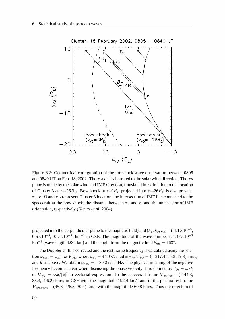
6 Statistical study of upstream waves
Figure 6.2: Geometrical configuration of the foreshock wave observation between 0805and 0840 UT on Feb. 18, 2002. Thex-axis is aberrated to the solar wind direction. Thexy
plane is made by the solar wind and IMF direction, translated inz direction to the locationof Cluster 3 atz=-26RE. Bow shock atz=0RE projected intoz=-26RE is also present.r0, r,D andeB represent Cluster 3 location, the intersection of IMF line connected to thespacecraft at the bow shock, the distance betweenr0 andr, and the unit vector of IMForientation, respectively (Narita et al.2004).
projected into the perpendicular plane to the magnetic field) and (kx, ky, kz) = (-1.1×10−3,0.6×10−3, -0.7×10⁻³) km−1 in GSE. The magnitude of the wave number is 1.47×10⁻³
km−1 (wavelength 4284 km) and the angle from the magnetic fieldθkB = 163.
The Doppler shift is corrected and the rest frame frequency is calculated using the rela-tionωrest = ωsc−k·V sw, whereωsc = 44.9×2πrad mHz,V sw = (−317.4, 55.8, 17.8) km/s,andk as above. We obtainωrest = −89.2 rad mHz. The physical meaning of the negativefrequency becomes clear when discussing the phase velocity. It is defined asVph = ω/k
or V ph = ωk/|k|2 in vectorial expression. In the spacecraft frameV ph(sc) = (-144.3,83.3, -96.2) km/s in GSE with the magnitude 192.4 km/s and in the plasma rest frameV ph(rest) = (45.6, -26.3, 30.4) km/s with the magnitude 60.8 km/s. Thus the direction of
80
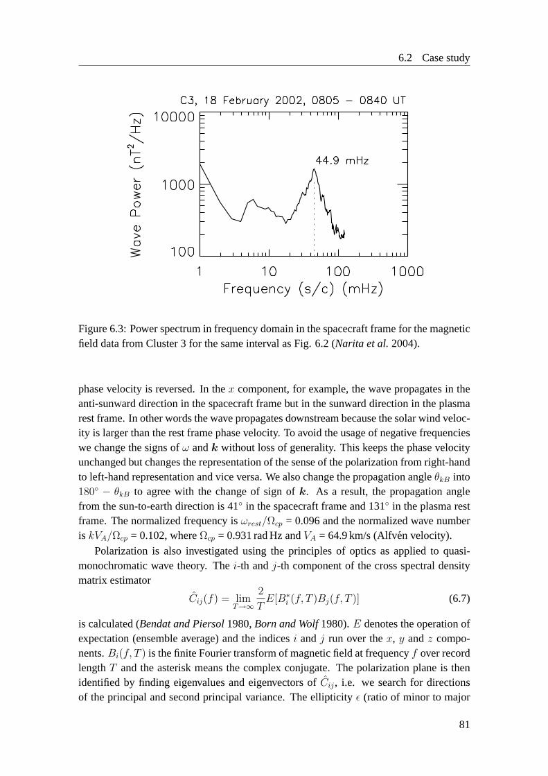
6.2 Case study
Figure 6.3: Power spectrum in frequency domain in the spacecraft frame for the magneticfield data from Cluster 3 for the same interval as Fig. 6.2 (Narita et al.2004).
phase velocity is reversed. In thex component, for example, the wave propagates in theanti-sunward direction in the spacecraft frame but in the sunward direction in the plasmarest frame. In other words the wave propagates downstream because the solar wind veloc-ity is larger than the rest frame phase velocity. To avoid the usage of negative frequencieswe change the signs ofω andk without loss of generality. This keeps the phase velocityunchanged but changes the representation of the sense of the polarization from right-handto left-hand representation and vice versa. We also change the propagation angleθkB into180 − θkB to agree with the change of sign ofk. As a result, the propagation anglefrom the sun-to-earth direction is 41 in the spacecraft frame and 131 in the plasma restframe. The normalized frequency isωrest/Ωcp = 0.096 and the normalized wave numberis kVA/Ωcp = 0.102, whereΩcp = 0.931 rad Hz andVA = 64.9 km/s (Alfven velocity).
Polarization is also investigated using the principles of optics as applied to quasi-monochromatic wave theory. Thei-th andj-th component of the cross spectral densitymatrix estimator
Cij(f) = limT→∞
2
TE[B∗
i (f, T )Bj(f, T )] (6.7)
is calculated (Bendat and Piersol1980,Born and Wolf1980).E denotes the operation ofexpectation (ensemble average) and the indicesi andj run over thex, y andz compo-nents.Bi(f, T ) is the finite Fourier transform of magnetic field at frequencyf over recordlengthT and the asterisk means the complex conjugate. The polarization plane is thenidentified by finding eigenvalues and eigenvectors ofCij, i.e. we search for directionsof the principal and second principal variance. The ellipticityε (ratio of minor to major
81

6 Statistical study of upstream waves
Figure 6.4: Wave power ink-space made by the wave telescope and the magnetic fielddata from all four Cluster for the same interval as Fig. 6.2.k⊥ is in the same direction asion bulk velocity projected into the perpendicular plane to the magnetic field (Narita etal. 2004).
axis in the polarization plane) is defined by Eq. (3.20) and Eq. (3.21). The ellipticity iscompared among different spacecraft and exhibit the result very close to one another infrequency domain, i.e. polarization is coherent for 100 km distance. We obtainε = 0.187for the given frequency, thus the wave is elliptically right-hand polarized in the spacecraftframe. In the plasma rest frame the sign ofε is changed, resulting from the reversal ofpropagation direction (Strictly speaking, the ellipticity in this context is an estimator andshould be expressed with a different symbol likeε, but we use simplyε to refer to it). Insummary, we have derived the following properties in the plasma rest frame: frequency∼ 0.1×Ωcp; wave number∼ 0.1×Ωcp/VA (also the wavelength of the order ofRE); phasevelocity∼ VA; propagation almost along the magnetic field (θkB = 17); and ellipticallyleft-handed polarization.
6.3 Statistical study
In the following statistical study we present various distributions of the foreshock waveproperties: frequencies, wave numbers, phase velocities, propagation directions, and po-larization, applying the analysis method introduced in the previous section. Intervals used
82

6.3 Statistical study
Figure 6.5: Histogram of magnitude of wave number (Narita et al.2004).
for the statistical study are selected as follows.(A) The mission phase for 100 km spacecraft separation (from 3 February 2002 to
17 June 2002) is selected in order to resolve waves into small wavelengths up to 200km; (B) Bow shock crossings are identified by searching for the following characteristics:(a) An increase in the magnetic field magnitude when moving from the upstream solarwind to the magnetosheath (typically by a factor of 2 to 4); (b) a decrease in the ionbulk speed; (c) an increase in the ion density. The ion bulk speed∼ 400 km/s is alsoreferred to in identifying the upstream region; (C) Moderately active fluctuation of themagnetic field is identified in the upstream region. For this purpose the variance of thefluctuation (defined in Section 2)0.05 ≤ σ2 ≤ 0.40 is imposed as a criterion; (D) Thegeometrical configuration is investigated and the intervals in the foreshock region areselected, applying the same method as described in the previous section.
For the selected intervals dominant frequencies are identified up to 0.5 Hz in the space-craft frame. 61 distinct waves from 36 events are selected under these criteria. Then wavenumbers, rest frame frequencies, and phase velocities are investigated. Ellipticities areinvestigated as well. Table 6.1 lists all the intervals and frequencies in the spacecraftframe. The histogram of magnitude of wave number is displayed in Fig. 6.5, which canbe derived only from multi-point measurements. We find that most of wave numbershave magnitude up to 2× 10⁻³ km−1. When normalized, this distribution exhibits a peakaround0.1× VA/Ωcp (discussed later).
Fig. 6.6 displays the spatial distribution of phase velocities in the plasma rest frameprojected into thexr plane in GSE (r =
√y2 + z2). Small circles filled in black are the
locations of wave observations and arrows starting from the circles are the phase velocities
83
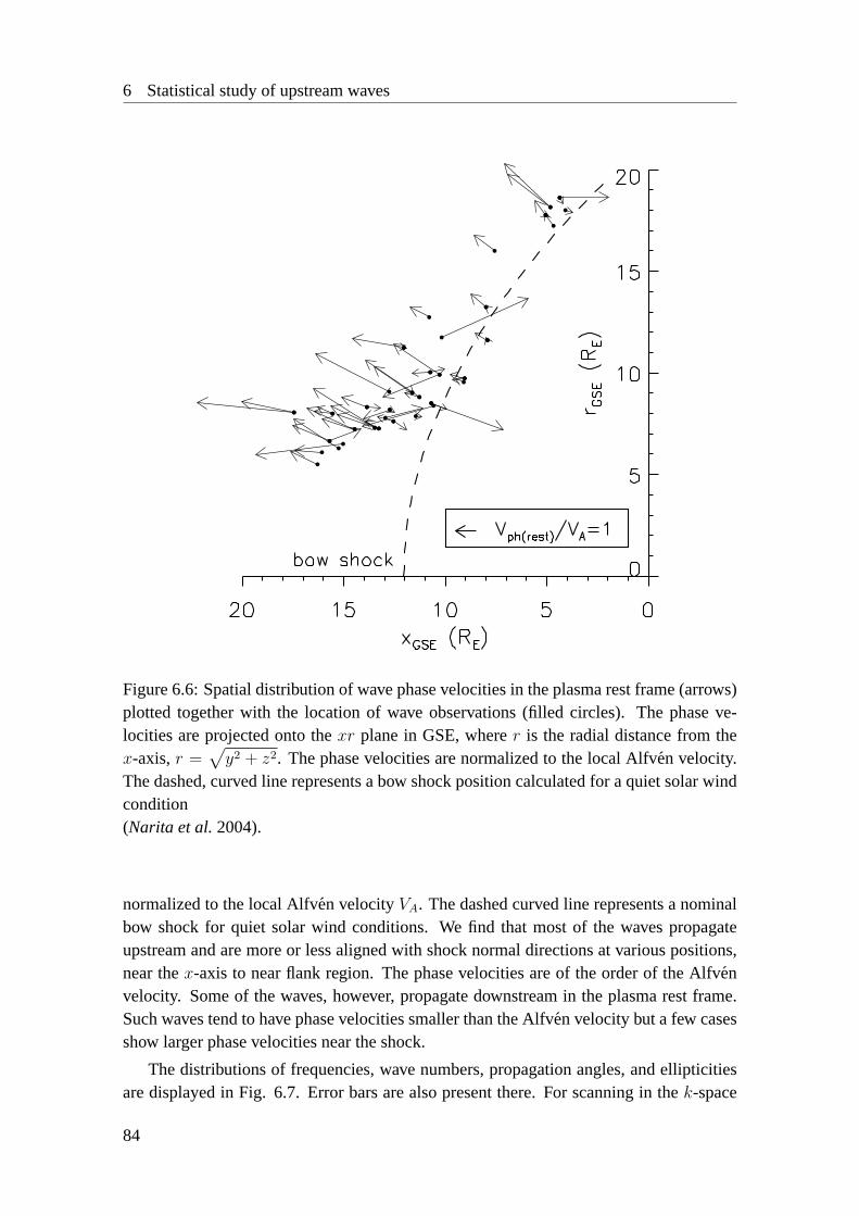
6 Statistical study of upstream waves
Figure 6.6: Spatial distribution of wave phase velocities in the plasma rest frame (arrows)plotted together with the location of wave observations (filled circles). The phase ve-locities are projected onto thexr plane in GSE, wherer is the radial distance from thex-axis,r =
√y2 + z2. The phase velocities are normalized to the local Alfven velocity.
The dashed, curved line represents a bow shock position calculated for a quiet solar windcondition(Narita et al.2004).
normalized to the local Alfven velocityVA. The dashed curved line represents a nominalbow shock for quiet solar wind conditions. We find that most of the waves propagateupstream and are more or less aligned with shock normal directions at various positions,near thex-axis to near flank region. The phase velocities are of the order of the Alfvenvelocity. Some of the waves, however, propagate downstream in the plasma rest frame.Such waves tend to have phase velocities smaller than the Alfven velocity but a few casesshow larger phase velocities near the shock.
The distributions of frequencies, wave numbers, propagation angles, and ellipticitiesare displayed in Fig. 6.7. Error bars are also present there. For scanning in thek-space
84

6.3 Statistical study
we use a spherical grid with 75× 60× 60 points in radial, azimuthal, and polar directionbetweenkmin = 0 km−1 andkmax = 5 × 10⁻³ km−1 for low-frequency waves up to100 mHz in the spacecraft frame, and between 0 km−1 and 25×10−3 km−1 for the restof frequencies. Mean|∆k| is thus about6.7 × 10−5 km−1 for low-frequency waves and3.3× 10−4 km−1 for high-frequency waves, and∆θkB is 3. Errors in the rest frame fre-quencies represent uncertainty in the Doppler shift, i.e.|∆k ·V sw|+ |k ·∆V sw|. We use∆k above and∆V sw which is calculated from mean absolute deviation of the ion velocityfor Cluster 3 CIS-HIA. We do not assign error bars in the ellipticities, since the eigenvec-tors of spectral density matrix are uniquely determined (without any uncertainty). Thereare, however, various methods to investigate polarization parameters. Comparison amongthese methods may give the error estimate in the ellipticities. The left panel is the distri-bution of normalized frequenciesωrest/Ωcp and magnitudes of normalized wave numberskVA/Ωcp. The signs ofωrest andk are already changed, since most of the frequenciesbecome negative after the Doppler shift correction. A magnified plot aroundω/Ωcp ∼ 0
andkVA/Ωcp ∼ 0.1 is also embedded in the left panel. The dotted, straight line representsAlfv en waves propagating along the magnetic field with the relationω/k = VA. Most ofthe waves are found atω/Ωcp ∼ 0.1 andkVA/Ωcp ∼ 0.1, therefore the major populationof the waves propagates at speeds below and around up to the Alfven velocity. Minorwaves are found up toω/Ωcp ∼ 5 andkVA/Ωcp ∼ 1.2. These waves are scattered intheω − k distribution. Some of them followω/k = VA and others deviate from it. Themiddle panel in Fig. 6.7 is the distribution of propagation anglesθkB versus frequencies.The first major population is found atθkB > 160 and the second major population isfound atθkB < 30. These two populations have small frequencies which correspondto the waves ofω/Ωcp ∼ 0.1 andkVA/Ωcp ∼ 0.1 in the left panel. Minor waves withrelatively large frequencies and wave numbers have propagation angles perpendicular tothe magnetic field rather than parallel/anti-parallel. The right panel in Fig. 6.7 is the dis-tribution of ellipticities. The ellipticities are located between -0.5 and 0.2. Major waveshave distribution centered slightly on the left-hand polarization side. Minor waves withlarger magnitude of frequencies tend to be left-handed for positive frequencies (upstreampropagation) and right-handed for negative frequencies (downstream propagation).
In summary, most of the waves have frequencies∼ 0.1 × Ωcp and wave numbers∼ 0.1 × Ωcp/VA. They propagate upstream almost parallel/anti-parallel to the magneticfield, at phase velocities close toVA with left-hand polarization. We interpret that thedominant waves represent Alfven waves because of good agreement in the phase velocityat low frequencies. Minor waves are also present, having propagation angles roughlyperpendicular to the magnetic field at various phase velocities. Some minor waves agreewith the dispersion relation of the Alfven wave (ω/k = VA) at larger frequencies and wavenumbers. We also examined if there is a possible relationship between frequencies orwave numbers and distances from the shock but they were relatively uniformly distributedand did not exhibit any clear signatures or organizations.
85

6 Statistical study of upstream waves
Figure 6.7: Distribution of rest frame frequencies, wave numbers, propagation angles, andellipticities in the plasma rest frame with error bar estimates. The small plot embeddedin the left panel is a magnified plot of the frequencies and the wave numbers near origin.The dotted, straight line in the left panel is a dispersion relation for the extended linearAlfv en waves (Narita et al.2004).
6.4 Discussion
Upstream propagation is dominating in the foreshock, as is expected from earlier casestudies. (Russell et al.1971,Hoppe et al.1981,Hoppe and Russell1983,Eastwood etal. 2002,Narita et al. 2003). We also identified rest frame frequencies∼ 0.1 × Ωcp
and wave numbers∼ 0.1 × Ωcp/VA (wavelengths of the order ofRE). These resultsconfirm the ISEE observations (Hoppe et al.1981,Hoppe and Russell1983) and implypropagation speeds close to Alfven velocity. If we restrict the observations to propagationangle parallel/anti-parallel to the magnetic field at frequency much smaller than the protoncyclotron frequency, we may conclude that the dominant waves in the foreshock propagateat about the Alfven speed. Taking account for the polarization analysis that waves are left-handed rather than right-handed, our results prefer the beam ion instability theory.
Some of the minor waves, despite larger wave numbers, had phase velocities close tothe Alfven velocity, whereas non-magnetohydrodynamic waves such as the ion cyclotronresonant waves or the cold plasma waves might be expected in this domain. These minorwaves tend to propagate perpendicular to the magnetic field. The waves propagatingalong the magnetic field in the foreshock region have been widely studied and discussed,but the perpendicular propagation may be important as well in understanding the physicalprocesses in this region.
86

6.5 Summary
6.5 Summary
Various properties of low-frequency waves such as frequencies, wave numbers, phase ve-locities, and polarization are investigated in the plasma rest frame in the upstream (fore-shock) region. Using Cluster observations, the wave telescope is applied to investigatethe wave numbers and the rest frame frequencies. One finds that most of the foreshockwaves propagate upstream along the magnetic field at phase velocities close to the Alfvenvelocity. We identify that frequencies are around0.1 × Ωcp and wave numbers around0.1× Ωcp/VA.
87

6 Statistical study of upstream waves
Table 6.1: Time intervals and dominant frequencies taken from 4-s and 1-s magnetic fielddata used in the statistical study of the foreshock waves .
Interval fsc(low) fsc(high)
mHz mHz2002-02-03 / 04:00-04:35 89.8 113.32002-02-11 / 22:00-22:35 50.8 160.22002-02-12 / 10:00-10:35 36.1 156.32002-02-12 / 12:00-12:35 40.0 101.62002-02-12 / 14:00-14:35 67.4 398.42002-02-13 / 16:00-16:35 88.9 308.62002-02-16 / 07:00-07:35 40.0 164.12002-02-18 / 08:05-08:40 44.9 312.52002-02-20 / 17:00-17:35 55.7 97.72002-02-20 / 22:00-22:35 50.8 101.62002-02-21 / 22:00-22:35 62.5 246.12002-02-26 / 20:30-21:05 44.9 269.52002-03-01 / 07:00-07:35 47.9 214.82002-03-06 / 00:30-01:05 36.1 433.62002-03-07 / 05:00-05:35 39.0 97.72002-03-09 / 12:00-12:35 30.3 425.82002-03-09 / 14:20-14:55 25.4 97.72002-03-09 / 16:00-16:35 27.3 175.82002-03-10 / 17:00-17:35 42.0 97.72002-03-11 / 20:00-20:35 46.9 210.92002-03-13 / 04:30-05:05 34.1 320.32002-03-16 / 13:00-13:35 35.1 97.72002-03-16 / 15:00-15:35 30.3 140.62002-03-26 / 17:50-18:25 29.3 453.12002-03-27 / 07:00-07:35 43.0 335.92002-03-29 / 18:00-18:35 114.3 308.62002-03-29 / 20:30-21:05 55.7 390.62002-04-02 / 04:00-04:35 81.1 160.12002-04-03 / 16:30-17:05 21.5 457.02002-04-27 / 02:00-02:35 43.9 97.72002-05-07 / 23:20-23:55 34.2 113.32002-05-13 / 14:50-15:25 50.8 457.02002-05-20 / 04:30-05:05 44.9 457.02002-05-20 / 06:00-06:35 37.1 406.3
88

6.5 Summary
2002-05-20 / 08:30-09:05 44.9 312.52002-05-22 / 11:20-11:55 41.0 457.0
89


7 Dispersion analysis of downstreamwaves
7.1 Introduction
In any experiments it is often said that case studies and statistical studies are comple-mentary to each other. The former method provides detailed information about whathappens in the selected case or event, while the latter identifies various populations thathave distinct aspects. Those methods applied to the upstream waves proved that the wavesrepresent the one driven by the (right-hand) ion beam instability and propagating towardupstream, where the beam is provided by the ion reflection at the shock and backstreamingagainst the incoming flow. According to the statistics in the previous chapter the majorityof the upstream waves exhibits this property.
Let us move onto the downstream region and apply those methods there. It is also ofinterest to ask how the upstream and the downstream waves are related to each other. Itshould be noted that this problem is not solved yet, for example, whether the upstreamwaves enter the magnetosheath as they are carried by the solar wind. Early studies onthe wave transmission across the bow shock also motivate this study. In the magneto-hydrodynamic (MHD) picture a wave incident on the front side of the bow shock givesrise to different kinds of MHD waves which diverge from the back of the shock: Alfvenwaves, magnetosonic waves, and an entropy wave. Their respective amplitudes are givenby solving the perturbed conservation relations across the shock. For example, an Alfvenwave upstream of the shock is transmitted into the downstream region with amplitudeenhanced by a factor about three (McKenzie and Westphal1969, 1970,Hassam1978)and an upstream magnetosonic wave is also enhanced across the shock (McKenzie andWestphal1969). Krauss-Varban and Omidi(1991, 1993) andKrauss-Varban(1994), onthe other hand, presented hybrid simulations of upstream and downstream waves at thequasi-parallel shock and argued that the upstream waves driven by the right-hand ionbeam instability are mode converted into the Alfven/ion cyclotron waves. As pointed outby Krauss-Varban et al.(1994b), when the scale of the waves approaches ion scales, akinetic treatment is necessary.
In this chapter we address the question of how wave dispersion characteristics arechanging when going from the upstream region through the bow shock toward the mag-netopause. A detailed characterization of wave dispersion properties is aimed for as
91

7 Dispersion analysis of downstream waves
Figure 7.1: Time series plot of magnetic field strength, ion density, and ion bulk veloc-ity observed by Cluster. The time interval shown is the same as Fig. 6.1 (Narita andGlassmeier2005).
they allow to discriminate between, for example, transmitted waves and locally gener-ated waves. Also, waves excited by the ion beam instability usually exhibit differentdispersion branches as theoretical studies indicate. Which branch is important can easilybe decided studying experimentally determined dispersion relations (Chapter 4).
Dispersion relations are determined from the magnetic field and ion measurementsmade by Cluster. Using a Fourier analysis in the time domain and the wave telescopeallows one to constructω-k-diagrams (frequency - wave number diagrams) in the plasmarest frame corrected for the Doppler shift.
For the present study we use data from the interval 0400-1000 UT on February 18,2002, when the spacecraft separation was about 100 km. Fig. 7.1 displays the magneticfield strength as well as the ion density and the bulk velocity. The Cluster s/c movedoutbound from the magnetosphere into the solar wind. The interval 0400-0500 UT coversobservations in the Earth’s magnetosphere, 0500-0800 UT the magnetosheath, 0800-0900UT the foreshock with several shock crossings, and 0900-1000 UT covers the solar wind(Fig. 7.2). We select four subintervals for the dispersion analysis: 0805-0840 UT forthe upstream (foreshock) waves (labeled as A), 0700-0735 UT the outer magnetosheathwaves (B), 0600-0635 UT the middle magnetosheath waves (C), and 0500-0535 UT theinner magnetosheath waves (D). The shock angle determined using the magnetic fieldcoplanarity theorem is17, that is the Cluster s/c traversed a quasi-parallel shock.
92

7.2 Dispersion analysis
Figure 7.2: Cluster orbit in the plane made by the solar wind direction (opposite to thex-axis in the plot) and interplanetary magnetic field direction. BS and MP stand for thebow shock and the magnetopause in this plane, respectively. The solid arrows representthe interplanetary magnetic field direction, and the solid arrow represents the Cluster orbit(Narita and Glassmeier2005).
7.2 Dispersion analysis
The analysis method follows Chapter 4. The wave power is calculated in the wave numberdomain at various frequencies using the wave telescope. Magnetic field data with 1s timeresolution are used in the analysis and the wave power is investigated at wavelengths downto 200 km. A Doppler shift of frequency is then corrected for the relation
ωrest = ωsc − k · V flow, (7.1)
whereωrest, ωsc, k, andV flow denote the wave angular frequency in the plasma rest frameof reference and in the spacecraft frame, wave vector, and plasma flow velocity vector,respectively. For the plasma flow velocity we use the ion bulk velocity data measuredby CIS-HIA, assuming that the background flow is stationary. It is worthwhile to notethat one needs to know the full wave vector to obtain the frequency in the plasma restframe. Only multi-point measurement of the Cluster s/c are up to now able to provide thisinformation.
In addition to the dispersion analysis we use a polarization analysis to identify thewave modes. The transverse magnetic field polarizationp is defined as (Fowler et al.
93

7 Dispersion analysis of downstream waves
1967)
p = tanφ = iδBy
δBx
, (7.2)
whereφ denotes the polarization angle determined from the cross spectral density matrixof the transverse magnetic field fluctuations, andδBy andδBx denote the minimum andmaximum transversal magnetic field variation, respectively. A valuep = +1 indicatesright-hand circular polarization with respect to the magnetic field direction, that is in thesame sense as the gyromotion of an electron,p = 0 linear polarization, andp = −1 left-hand circular polarization, that is the same rotation sense as the ion gyromotion. Becausep depends on frequency (Stix 1992), the sign of polarization is changed when the restframe frequency is negative (anomalous Doppler shift).
The results of the dispersion and polarization analysis are displayed in Fig. 7.3. Thedifference of the background magnetic field strength and the plasma density between theforeshock and the magnetosheath results in difference of normalized frequency - wavenumber range available: a higher Alfven speed in the magnetosheath than in the foreshockresults in a smaller value of normalized wave number. Due to the anomalous Dopplershift the signs of the rest frame frequencies are reversed to bring most of them into thepositive regime in all the panels. Accordingly, the propagation angle is changed asθkB →180−θkB. For scanning in thek-space we use a spherical grid with75×60×60 points inradial, azimuthal, and polar direction up to Nyquist wave numberkNy = 3 × 10⁻²km−1.The uncertainty of wave number is thus about∆k = 4× 10⁻⁴km−1 for the wave numbermagnitude and∆θkB = 3 for the propagation angle with respect to the magnetic field.The uncertainty in the rest frame frequency represents the one in the Doppler shift, i.e.|∆ωre
ωre| ≤ |∆k
k| + |∆V
V|. We use∆V which is calculated from mean absolute deviation of
the CIS-HIA bulk velocity data. The results of the polarization analysis are over-plotted.We classify the polarization as right-handed (RH) ifp > 0.176 (i.e. φ > 10), left-handed(LH) if p < −0.176 (i.e. φ < −10), and linear (Lin) if−0.176 ≤ p ≤ 0.176.
The upstream waves exhibit two branches [Fig. 7.3A]. Branch 1 starts at(ω, k) '(0, 0) and extends up to about(ω, k) ' (1.5, 1.5). Branch 2 reaches from(ω, k) '(−1.0, 0.0) to about(ω, k) ' (0.5, 0.2 − 0.3), intersecting branch 1 at(0.1, 0.1 − 0.2).Propagation is slightly off-angle at20 − 30 for almost all wave numbers. Only forvery small wave numbers it is perpendicular to the background magnetic field. Variouspolarizations are detected with the linear and the right-hand polarization dominating (Fig.7.4A).
In the outer magnetosheath (near the shock) frequencies are small (at most 0.4) atvarious wave numbers (Fig. 7.3B). Propagation is oblique to perpendicular with a fewnearly parallel cases (12 < θkB < 20); the polarization is clearly linear (Fig. 7.4B).The nearly parallel propagating waves exhibit phase speeds about 0.1 - 0.2 as large as theAlfv en speed with left-hand polarization (−0.2 < p < −0.6), which may represent ioncyclotron waves.
In the middle magnetosheath the dispersion appears as an almost horizontal line atabout zero frequency, though the frequencies deviate a little from zero at wave numbers
94

7.2 Dispersion analysis
Figure 7.3: Dispersion relations and propagation angles with error bars in the foreshock(0805-0840 UT), in the outer magnetosheath (0700-0735 UT), in the middle magne-tosheath (0600-0635 UT), in the inner magnetosheath (0500-0535 UT). Frequency andwave number are normalized to proton cyclotron frequencyΩcp and inverse of ion inertialscaleΩcp/VA, whereVA stands for Alfven velocity. The quantities areΩcp = 0.92 (radHz) andVA = 61.84 (km/s) for in the foreshock (A),Ωcp = 1.99 (rad Hz) andVA = 59.56
(km/s) in the outer magnetosheath (B),Ωcp = 1.84 (rad Hz) andVA = 57.50 (km/s) in themiddle magnetosheath (C), andΩcp = 2.01 (rad Hz) andVA = 82.53 (km/s) in the innermagnetosheath (D) (Narita and Glassmeier2005).
0.4 − 0.6 (Fig. 7.3C). Wave vectors are clearly perpendicular to the magnetic field andpredominantly oriented in the direction from the sun to the Earth (kx < 0 in the GSEcoordinate system); the polarization is linear (Fig. 7.4C).
The inner magnetosheath waves (near the magnetopause) exhibit scattered frequenciesand propagation angles (Fig. 7.3D). Average propagation angles tend to be90 − 120;
95

7 Dispersion analysis of downstream waves
Figure 7.4: Histograms of magnetic field polarization at various frequencies for the sameevents as Fig. 7.3 (Narita and Glassmeier2005).
the polarization is still clearly linear (Fig. 7.4D).
7.3 Discussion
Two intersecting branches in the upstream wave dispersion were already identified inChapter 4. The first branch represents the right-hand whistler mode and the second branchthe beam resonant mode in which the wave is propagating together with the ion beam.Polarization is found to be linear to right-hand, which is also in accord with the whistlerbranch.
In the outer magnetosheath these properties are lost except for the perpendicular prop-agation at very small wave numbers. Mirror modes are dominating in the middle mag-
96

7.3 Discussion
Table 7.1: Plasmaβ, temperature anisotropyT⊥/T‖, and transport ratioR = cosψnb
for different regions investigated, whereψnb denotes the phase angle between the plasmadensity and the magnetic field fluctuations (Narita and Glassmeier2005).
Region β T⊥/T‖ R
Foreshock 4.838 0.702 0.974Outer Sheath 5.982 1.229 -0.977Middle Sheath 8.012 1.258 -0.893Inner Sheath 3.425 1.217 -0.885
netosheath, since the frequencies are almost zero, the wave vectors are perpendicular tothe background magnetic field, polarization is linear, and furthermore, the fluctuations ofthe magnetic field are anti-correlated to the plasma density fluctuations (Table 7.1). Theouter magnetosheath waves seem to be in a transient state toward the mirror mode. Theremay exist waves other than the mirror mode in the outer magnetosheath that fade towardthe middle magnetosheath.Hubert et al.(1998) argued using ISEE observations that themagnetosheath waves represent the ion cyclotron waves near the shock and the mirrormode structures closer to the magnetopause.Denton et al.(1998) also presented Alfven-like modes in the outer magnetosheath. The ion cyclotron waves are a likely candidate.We speculate that the outer magnetosheath waves are a mixture of the mirror modes andion cyclotron waves propagating toward the flank region.
In the inner magnetosheath the mirror mode properties are distorted such that fre-quencies (and also phase speeds) deviate from zero and propagation angles deviate from90, while they keep the linear polarization. The mirror modes with finite frequenciesand phase speeds were already found byOmidi and Winske(1995). They used a one-dimensional hybrid simulation to model the entire region from the solar wind to themagnetic boundary and found mirror mode waves that are phase standing relative to themagnetic boundary, which implies that the phase standing waves must have a finite prop-agation speed in the plasma rest frame. These waves are referred to as ‘MIrror AndslOW’ or MIAOW waves and observed near the magnetopauseBalikhin et al. (2001).The vicinity of the magnetopause seems to modify the mirror mode characteristics. Thefinite propagation of the mirror mode in oblique direction may be due to a variety ofprocesses, including nonlinearity (Stasiewicz2004a), inhomogeneous background statesuch as density gradients (Hasegawa1969,Pokhotelov et al.2001), or eigenmode of themagnetosheath (Johnson and Cheng1997).
Table 7.1 displays plasma parameterβ (ratio of thermal to magnetic pressure,pth/pB),temperature anisotropyT⊥/T‖, and transport ratioR for the time intervals under investiga-tion. Plasmaβ is greater than unity (thermal pressure dominant) throughout the intervals,though it shows a variation, being enhanced from about 4 in the foreshock to about 8toward the middle magnetosheath and diminished to about 3 in the inner magnetosheath.The enhancement ofβ in the middle magnetosheath stems from the diminished IMF by
97

7 Dispersion analysis of downstream waves
[t]
Figure 7.5: Schematic illustration of wave habitats. Arrows represent wave vectors. ‘IC’and ‘MM’ stand for ion cyclotron waves and mirror modes, respectively (Narita andGlassmeier2005).
about 20% detected by the ACE spacecraft. Temperature anisotropyT⊥/T‖, which isratio of perpendicular to parallel temperature with respect to the background magneticfield direction, becomes parallel dominant (about 0.7) in the foreshock to perpendiculardominant in the magnetosheath (about 1.2). Anisotropy is nearly constant in the mag-netosheath. Transport ratioR represents the cosine of the phase angle between the den-sity and magnetic field strength variations (Denton et al.1998), and it is averaged overfrequencies under the condition of the coherence greater than 0.7 between the two vari-ations. It shows the value about 1 (correlated density and magnetic field variations) inthe foreshock and -1 (anti-correlated variations) in the magnetosheath. The foreshockwaves exhibit the property of the fast magnetosonic waves which is consistent with theright-hand beam instability and that the magnetosheath waves exhibit predominantly themirror mode characteristics. The mirror mode interpretation in the magnetosheath is alsosupported by the high plasmaβ and the large perpendicular temperature observed.
Fig. 7.5 illustrates wave habitats and wave vectors derived from our study. The up-stream waves are driven by the ion beam instability with wave vectors oriented toward up-stream and almost parallel to the background magnetic field. In the outer magnetosheaththere are a minor contribution of the ion cyclotron waves (IC) and a major contribution ofthe mirror modes (MM). The middle magnetosheath exhibits the clearest mirror modes.In the inner magnetosheath the mirror mode properties are distorted probably due to ad-ditional effects such as nonlinear, inhomogeneous background, or eigenmode effects.
From the viewpoint of the problem of the wave transmission or mode conversionacross the shock, we find that the fast mode is not present in the downstream region andthat the ion cyclotron waves do not dominate either. The mirror modes and the ion cy-
98

7.4 Summary
clotron waves in the magnetosheath are believed to originate in the temperature anisotropyprovided by the ion reflection at the shock, and it seems that the wave transmission ormode conversion across the shock does not apply to the Earth’s bow shock case. But wenote thatKrauss-Varban and Omidi(1993) used a low plasmaβ condition for their simu-lation study, while highβ dominates in the present case. Therefore, it is worthwhile to doa numerical simulation under the highβ condition and to compare with our result, whichwill be a subject of future investigation.
7.4 Summary
The dispersion analysis and additional investigations on the polarization and the trans-port ratio suggest that the upstream waves lose their identity as they are convected bythe background flow and that they are not transmitted into the magnetosheath. Perhapsthey are lost near or at the shock. In the outer magnetosheath the mirror modes and theion cyclotron waves are likely to coexist, both of which are known to be driven by pres-sure anisotropy. In the middle magnetosheath only the mirror modes dominate, while inthe inner magnetosheath their properties are distorted to have finite frequencies and wavevectors oblique to the magnetic field. The mirror modes are subject to nonlinear or inho-mogeneous effect near the magnetopause. Further investigations on dispersion relation,propagation and polarization characteristics, and transport ratios in various regions of theforeshock and the magnetosheath will verify our result. On the other hand, theoreticalinvestigations under various conditions (e.g. high plasmaβ) will improve our compre-hension about the mode transmission or conversion problem.
99


8 Statistical study of downstreamwaves
8.1 Introduction
The dispersion analysis presented in Chapter 7 suggests that the mirror modes dominate inthe downstream region, but on the other hand it has been understood that their frequenciesare not exactly zero. This chapter presents a statistical study of the downstream waves andattempts to determine typical values of wave frequencies, wave number, and so on, fordifferent regions from the upstream to the downstream region, and for the quasi-paralleland the quasi-perpendicular shock regime.
The propagation pattern presented in Chapter 6 is also extended to the downstreamregion. Matsuoka et al.(2000) andSchafer et al.(2005) showed that Alfvenic waves inthe magnetosheath propagate in the same direction as the plasma flow in a draped field,that is anti-sunward and away from the sun-Earth line. Yet, little is known about howthe waves propagate at what speed nor whether the propagation properties are similaror different between the quasi-parallel and the quasi-perpendicular shock regimes. Thisstems from the fact that wave vectors were hardly determined in single or at best twospacecraft observations, preventing one from determining phase velocities.
8.2 Statistical study
In order to perform the statistical study the following criteria and methods are used. About50 upstream events and about 200 downstream events observed by the Cluster s/c areinvestigated. Since the selection procedure for the upstream wave events was alreadypresented in the foreshock wave study (Chapter 6), we describe here the downstreamwave events in detail.
The mission phase with a 100 km spacecraft separation, that is the time interval fromFebruary 3 to June 17, 2002 is selected to resolve wavelengths down to 200 km. TheCluster s/c observed in the post-noon to the dawn sector of the magnetosheath during thismission phase.
The magnetosheath region has been identified from bow shock and magnetopausecrossings, by investigating magnetic field data from FGM instrument and ion data ob-
101

8 Statistical study of downstream waves
Figure 8.1: Time series plot of magnetic field strength, ion number density, ion bulkspeed, and plasma beta parallel (dotted) and perpendicular (dashed) to the magnetic field,observed by Cluster 3 from 03:00 UT (solar wind region) to 10:00 UT (magnetosphere),February 3, 2002 (Narita et al.2006a).
tained by CIS-HIA and CIS-CODIF instrument. Identification of the bow shock crossingfor the inbound spacecraft motion is based on a sudden increase of the magnetic fieldwithin the spacecraft spin period (4s) by a factor2−4, accompanied by an increase of theion density, and a decrease of the ion bulk speed. For the inbound magnetopause crossingan increase of the magnetic field, a significant decrease of the ion density and a moderatedecrease of the ion bulk speed are used as an indicator. Fig. 8.1 displays as an examplethe magnetosheath observations made on February 3, 2002. The spacecraft motion wasinbound from the solar wind to the magnetosphere.
Three intervals are chosen as the outer, the middle, and the inner magnetosheath regionfrom each traversal with the intervals equidistantly positioned in the time domain. Fig. 8.1displays an example of the interval selection. For the outer and the inner magnetosheathintervals as close as possible to the bow shock and to the magnetopause, respectively,have been selected. During some orbits only either the bow shock or the magnetopause
102

8.2 Statistical study
crossing could be identified due to a lack of data. In such a case we drop the inner orthe outer region and pick up the remaining two intervals to analyze as many events aspossible. As a result of the selection procedure we obtain 84 magnetosheath traversalswith 197 intervals for the statistical study (Table 8.1).
To determine whether the observations are made closer to the quasi-parallel or thequasi-perpendicular shock we introduce a new coordinate system, the solar wind system,in which the basis vectorsex, ey, andez are given by
ex = −ev (8.1)
ey = ez × ex (8.2)
ez =Bs
|Bs|ev × eb, (8.3)
whereev andeb are the unit vectors of the solar wind velocity and the interplanetarymagnetic field (IMF), andBs is the sunward component of the IMF. Fig. 8.2 shows twoexamples of how the coordinate system is transformed. First thex-axis is oriented anti-parallel to the solar wind direction, then the system is rotated about thex-axis so that thexy-plane is identical with the plane spanned by the solar wind and the IMF directions.There are two possibilities to determine they-direction, closer to or distant from the IMFdirection. We choose they-direction which is oriented closer to the IMF direction ifBs < 0 (Fig. 8.2 top) and to the opposite direction ifBs > 0 (Fig. 8.2 bottom), so thatthe IMF line is always tangential to the bow shock in they > 0 regime. To determinethe solar wind and the IMF directions, ion and magnetic field data from the ACE s/c(Stone et al.1998) are used. Since ACE monitors the solar wind at a distance of about200 to 250RE (1RE = 6370 km) in front of the Earth, its observation time is shiftedforward by 60 minutes to compensate any time delay between the ACE position andthe Earth. The ACE data are averaged over 90 minutes. We associate the observationswith the near quasi-perpendicular shock regime if the sign of they-component of theCluster position in the newly introduced solar wind coordinate system is positive andvice versa. This coordinate system is equivalent to the three axes of the magnetosheath -interplanetary medium (MIPM) reference frame (Verigin et al.2006). The advantage touse this coordinate system is that one can determine the shock regime corresponding togiven Cluster observations even if shock crossing data are not available.
Fig. 8.3 shows an example of the Cluster orbit in the solar wind system for the sameinterval as Fig. 8.1. The Cluster trajectory is located in the near quasi-parallel shockregime. Note that this classification is based on determination of the upstream conditionsand does not work if the IMF cone angle is close to0 or 90 and that it is different fromthe one based on the shock angle determination using the magnetic field coplanarity the-orem, although both results agree well with each other in the statistical study. In the casedisplayed in Fig. 8.3, we obtainθBn = 13 (quasi-parallel shock) using the coplanaritytheorem for the shock crossing, where the Alfven Mach number is about18.
For any of the events the dominant frequency is determined using the power spectrumof the magnetic field in the spacecraft frame. We use 1s- and 4s-averaged magnetic field
103

8 Statistical study of downstream waves
Figure 8.2: Two sketches of the solar wind coordinate system for IMF with a negativesunward component (Bs < 0) and with a positive component (Bs > 0) (Narita et al.2006a).
data. The 4s-data are used to compare with CIS observations available with the corre-sponding time resolution. Fig. 8.4 shows the wave power in the frequency domain forthe example case. The wave powerP (f) is compared with the power lawP ∝ f−α (ref-erence wave power), whereP is the wave power,f is the frequency, andα is a positivevalue determined by fitting of the spectrum. From the power spectrum the frequency isidentified as the dominant frequency where the measured wave power deviates most fromthe reference wave power. In the example case we obtain 41 mHz.
The polarization about the magnetic field is investigated. We define the magneticpolarizationp following the ellipticity defined byFowler et al.(1967), which is calcu-lated from the cross spectral density matrix. In the investigation the basis vectors of thecross spectral density matrix of the magnetic field fluctuation are oriented to the directionof principal and minimal magnetic field variation in the plane perpendicular to the back-ground magnetic field. A value ofp = 1 denotes the right-hand circular polarization whenviewed into the magnetic field direction,p = 0 the linear polarization andp = −1 theleft-hand polarization. Under this definition a right-hand mode propagating either parallelor anti-parallel to the magnetic field possesses fluctuating field vectors that rotate in thesame sense as the gyro-motion of an electron (Eq. 7.2).
104
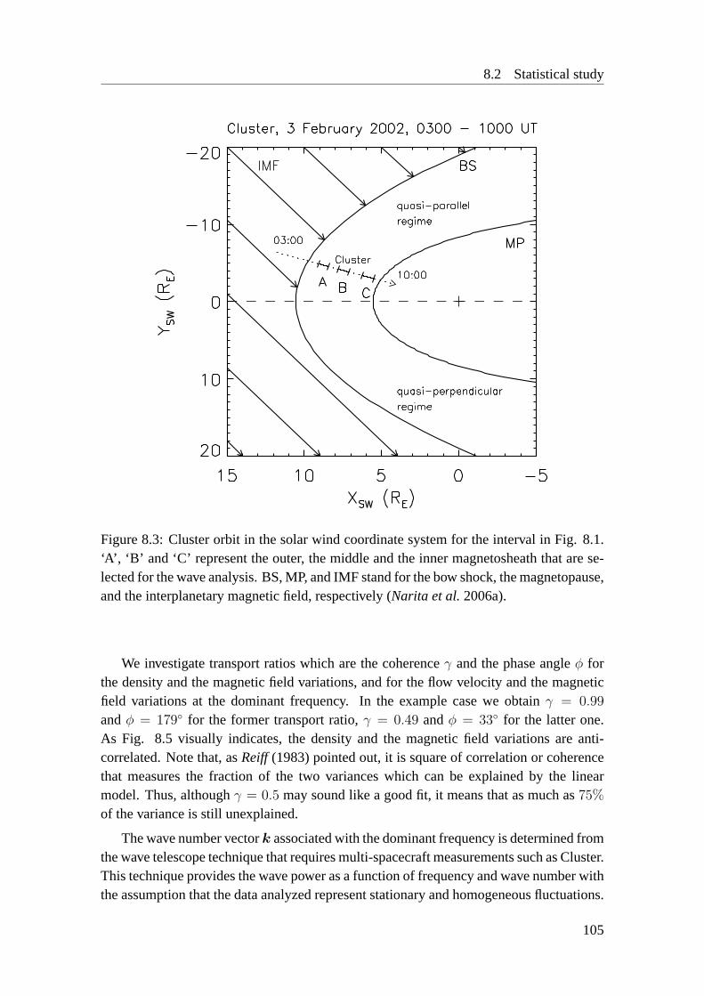
8.2 Statistical study
Figure 8.3: Cluster orbit in the solar wind coordinate system for the interval in Fig. 8.1.‘A’, ‘B’ and ‘C’ represent the outer, the middle and the inner magnetosheath that are se-lected for the wave analysis. BS, MP, and IMF stand for the bow shock, the magnetopause,and the interplanetary magnetic field, respectively (Narita et al.2006a).
We investigate transport ratios which are the coherenceγ and the phase angleφ forthe density and the magnetic field variations, and for the flow velocity and the magneticfield variations at the dominant frequency. In the example case we obtainγ = 0.99
andφ = 179 for the former transport ratio,γ = 0.49 andφ = 33 for the latter one.As Fig. 8.5 visually indicates, the density and the magnetic field variations are anti-correlated. Note that, asReiff (1983) pointed out, it is square of correlation or coherencethat measures the fraction of the two variances which can be explained by the linearmodel. Thus, althoughγ = 0.5 may sound like a good fit, it means that as much as75%
of the variance is still unexplained.
The wave number vectork associated with the dominant frequency is determined fromthe wave telescope technique that requires multi-spacecraft measurements such as Cluster.This technique provides the wave power as a function of frequency and wave number withthe assumption that the data analyzed represent stationary and homogeneous fluctuations.
105

8 Statistical study of downstream waves
Figure 8.4: Wave power as a function of spacecraft frame frequency calculated frommagnetic field data of Cluster 3 for the interval C in Fig. 8.1. The straight line shows thewave power fitted by the power lawP ∝ f−α. The dominant frequency is found at 41mHz (Narita et al.2006a).
Figure 8.5: Time series plot of the magnetic field magnitude (thick line) and the ion num-ber density (thin line) measured by Cluster 3 for the interval C in Fig. 8.1. A clear anti-correlation between the two fluctuations indicates the mirror mode in the magnetosheath(Narita et al.2006a).
Fig. 8.6 displays the wave power in thek-domain for the example case. Maximum poweris detected at(k‖, k⊥) = (−3.67 × 10⁻⁴, 3.64 × 10⁻³) km−1 at a wavelength of 1700km, and the angleθkB between the wave vectork and the magnetic field is96 (cf. ioninertial length is 270 km and thermal ion gyro-radius is 489 km for the interval underinvestigation).
106

8.2 Statistical study
Figure 8.6: Wave power as a function of wave number, parallel and perpendicular to themean magnetic field, at spacecraft frame frequency 41 mHz. The wave power is calculatedby the wave telescope technique, and peaks in the perpendicular direction. (Narita et al.2006a).
It should be noted here that a proper Doppler shift correction requires knowledge ofthe wave vectork. Only observations from the four Cluster s/c allow to determinek un-ambiguously with techniques such as the wave telescope. Using the Doppler shift relationωrest = ωsc−k·V flow we calculate the rest frame frequency. Hereωrest andωsc denote theangular frequency in the rest frame and in the spacecraft frame, respectively, andV flow
the plasma flow velocity. CIS measurements of the ion bulk velocity are used to determineV flow. We then calculate the wave phase velocity in the rest frame viaV ph = ωrestk/k
2.In our example case we obtainωrest = 13 rad mHz andV ph = (−0.3, 3.4) km/s paral-lel and perpendicular to the background magnetic field, or(−3.4, 0.0,−0.7) km/s in theGSE system. These quantities are intrinsic and not influenced by convection due to thebackground plasma flow.
Upstream waves are investigated in the same way as described above for the magne-tosheath waves. The waves upstream of the quasi-parallel shock represent the foreshockwaves. Based on the event selection criteria in the foreshock wave study (Chapter 6) weidentify 36 events for the foreshock (Table 6.1) and 19 events for the quasi-perpendicularshock upstream waves (Table 8.2).
107
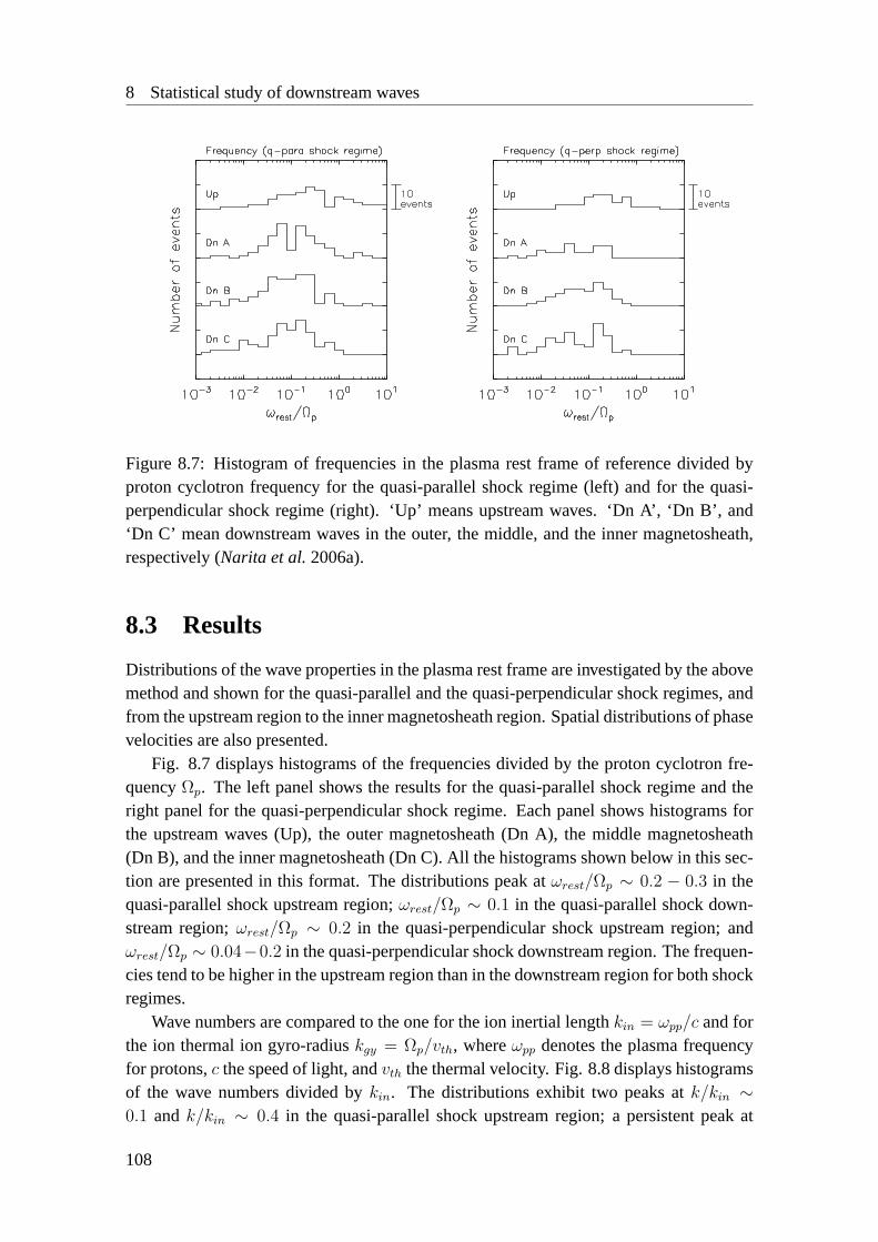
8 Statistical study of downstream waves
Figure 8.7: Histogram of frequencies in the plasma rest frame of reference divided byproton cyclotron frequency for the quasi-parallel shock regime (left) and for the quasi-perpendicular shock regime (right). ‘Up’ means upstream waves. ‘Dn A’, ‘Dn B’, and‘Dn C’ mean downstream waves in the outer, the middle, and the inner magnetosheath,respectively (Narita et al.2006a).
8.3 Results
Distributions of the wave properties in the plasma rest frame are investigated by the abovemethod and shown for the quasi-parallel and the quasi-perpendicular shock regimes, andfrom the upstream region to the inner magnetosheath region. Spatial distributions of phasevelocities are also presented.
Fig. 8.7 displays histograms of the frequencies divided by the proton cyclotron fre-quencyΩp. The left panel shows the results for the quasi-parallel shock regime and theright panel for the quasi-perpendicular shock regime. Each panel shows histograms forthe upstream waves (Up), the outer magnetosheath (Dn A), the middle magnetosheath(Dn B), and the inner magnetosheath (Dn C). All the histograms shown below in this sec-tion are presented in this format. The distributions peak atωrest/Ωp ∼ 0.2 − 0.3 in thequasi-parallel shock upstream region;ωrest/Ωp ∼ 0.1 in the quasi-parallel shock down-stream region;ωrest/Ωp ∼ 0.2 in the quasi-perpendicular shock upstream region; andωrest/Ωp ∼ 0.04−0.2 in the quasi-perpendicular shock downstream region. The frequen-cies tend to be higher in the upstream region than in the downstream region for both shockregimes.
Wave numbers are compared to the one for the ion inertial lengthkin = ωpp/c and forthe ion thermal ion gyro-radiuskgy = Ωp/vth, whereωpp denotes the plasma frequencyfor protons,c the speed of light, andvth the thermal velocity. Fig. 8.8 displays histogramsof the wave numbers divided bykin. The distributions exhibit two peaks atk/kin ∼0.1 andk/kin ∼ 0.4 in the quasi-parallel shock upstream region; a persistent peak at
108

8.3 Results
Figure 8.8: Histogram of wave numbers divided by ion inertial wave numberωpp/c. Panelformat is the same as Fig. 8.7 (Narita et al.2006a).
k/kin ∼ 0.1 − 0.2 in the quasi-parallel shock downstream region; two populations up tok/kin ∼ 1 andk/kin ∼ 0.3−0.4 in the quasi-perpendicular shock upstream region; and apersistent peak atk/kin ∼ 0.1−0.2 in the quasi-perpendicular shock downstream region.Fig. 8.9 displays histograms of the wave numbers divided bykgy. The distributionsexhibit two peaks atk/kgy ∼ 0.1 andk/kgy ∼ 0.5 − 0.7 in the quasi-parallel shockupstream region; and a persistent peak atk/kgy ∼ 0.2 − 0.6 in the quasi-parallel shockdownstream region and a peak atk/kgy ∼ 1 in the inner magnetosheath; two peaks atk/kgy ∼ 0.06 andk/kgy ∼ 0.4 in the quasi-perpendicular shock upstream region; and apeak atk/kgy ∼ 0.2− 0.4 in the quasi-perpendicular shock downstream region.
Phase velocities are compared to three characteristic propagation speeds in magneto-hydrodynamics: fast, intermediate, and slow mode speed. Their values are dependent onthe background magnetic field, density and temperature, and propagation direction. Wecalculate these speeds using the background quantities given by the FGM and the CISmeasurements and the propagation angle determined by the wave telescope technique.Fig. 8.10 displays histograms of the phase velocities divided by the fast mode speedVf .The distributions exhibit peaks atVph/Vf ∼ 1 in the quasi-parallel shock upstream re-gion; Vph/Vf ∼ 0.1 − 0.4 in the quasi-parallel shock downstream region;Vph/Vf ∼ 1
in the quasi-perpendicular shock upstream region; andVph/Vf ∼ 0.1 − 0.7 in the quasi-perpendicular shock downstream region. Fig. 8.11 displays the ones divided by the in-termediate mode speedVi. The distributions exhibit peaks atVph/Vi ∼ 0.6 − 0.7 and2− 3 in the quasi-parallel shock upstream region,Vph/Vi ∼ 1 in the quasi-parallel shockdownstream region;Vph/Vi ∼ 1 in the quasi-perpendicular shock upstream region; andVph/Vi ∼ 1 in the quasi-perpendicular shock downstream region. Fig. 8.12 displays theones divided by the slow mode speedVs. Since the phase velocities of the slow mode are
109

8 Statistical study of downstream waves
Figure 8.9: Histogram of wave numbers divided by the thermal ion gyro-wave number.Panel format is the same as Fig. 8.7 (Narita et al.2006a).
Figure 8.10: Histogram of phase velocities in the plasma rest frame divided by the onefor the fast mode. Panel format is the same as Fig. 8.7 (Narita et al.2006a).
generally close to that of the intermediate mode for the highβ plasma (e.g. Friedrichsdiagram inKivelson(1995)), the distributions exhibit similar peaks to the intermediatemode case:Vph/Vs ∼ 2 − 3 in the quasi-parallel shock upstream region;Vph/Vs ∼ 1 inthe quasi-parallel shock downstream region;Vph/Vs ∼ 1 − 2 in the quasi-perpendicularshock upstream region; andVph/Vs ∼ 1 in the quasi-perpendicular shock downstreamregion. The inner magnetosheath in the quasi-parallel shock regime exhibits also a peakatVph/Vi ∼ 3 andVph/Vs ∼ 4.
110

8.3 Results
Figure 8.11: Histogram of phase velocities in the plasma rest frame divided by the onefor the intermediate mode. Panel format is the same as Fig. 8.7 (Narita et al.2006a).
Figure 8.12: Histogram of phase velocities in the plasma rest frame divided by the onefor the slow mode. Panel format is the same as Fig. 8.7 (Narita et al.2006a).
Fig. 8.13 displays histograms of the propagation angles with respect to the back-ground magnetic field. They are markedly different between the upstream region and thedownstream region and show a similar trend in the both shock regimes. The upstreamwaves propagate almost parallel to the background magnetic field. In the outer magne-tosheath the distribution exhibits a slight peak in the perpendicular direction. Toward themagnetopause this peak becomes clearer. The quasi-perpendicular shock upstream wavesalso exhibit perpendicular and anti-parallel propagation.
111

8 Statistical study of downstream waves
Figure 8.13: Histogram of angles between the wave vector and the background magneticfield. Panel format is the same as Fig. 8.7 (Narita et al.2006a).
Figure 8.14: Histogram of magnetic polarization. Panel format is the same as Fig. 8.7(Narita et al.2006a).
Fig. 8.14 displays histograms of the magnetic polarization. In the quasi-parallel shockupstream region it s broadly distributed from left-hand (p = −1) to right-hand polariza-tion (p = +1), while in the downstream region the linear polarization (p = 0) is enhanced.A similar tendency is found in the quasi-perpendicular shock regime, too.
The distributions of the phase angles between the density and the magnetic field vari-ations (φNB) are displayed in Fig. 8.15; and the one between the plasma bulk velocityand the magnetic field variations (φV B) in Fig. 8.16. They are calculated under the condi-tion that their respective coherence is larger than 0.7. The quasi-parallel shock upstream
112
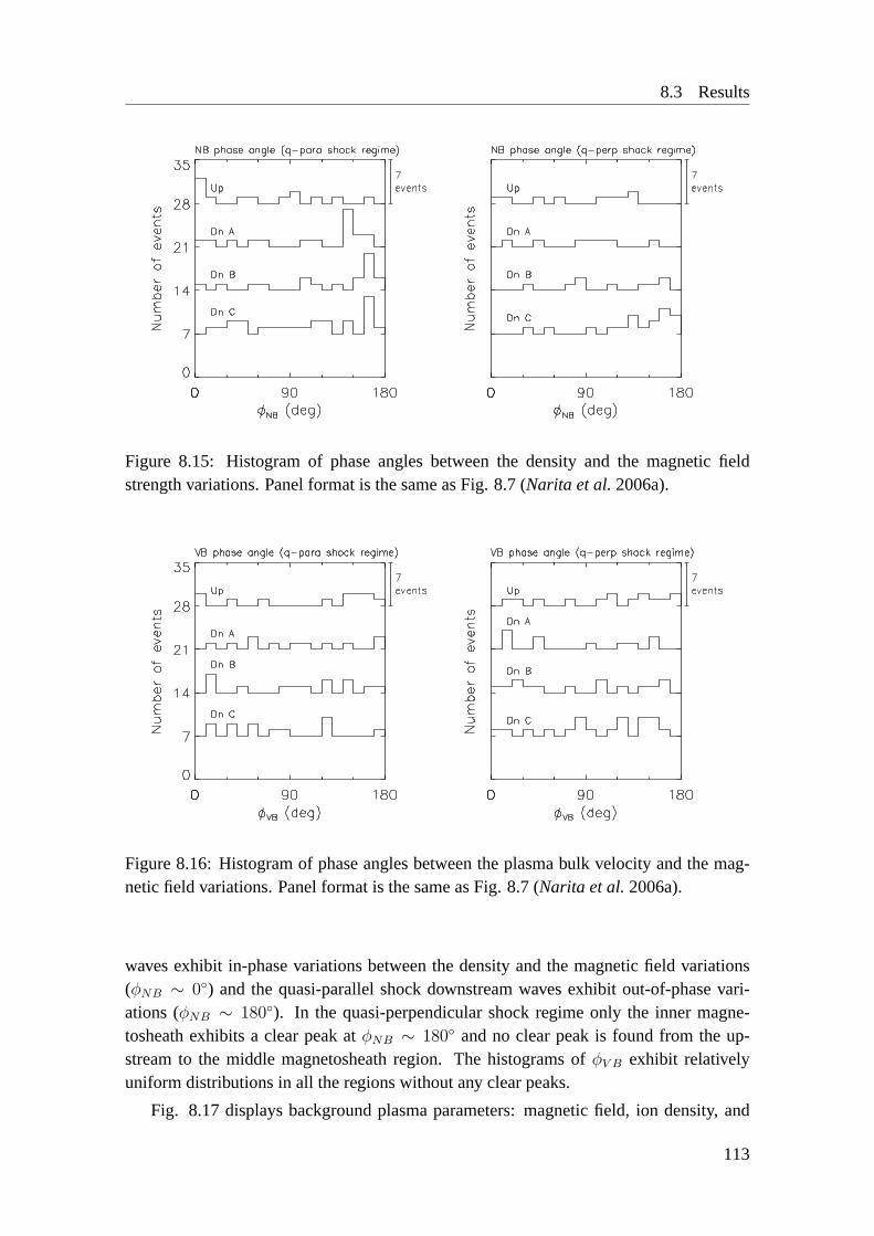
8.3 Results
Figure 8.15: Histogram of phase angles between the density and the magnetic fieldstrength variations. Panel format is the same as Fig. 8.7 (Narita et al.2006a).
Figure 8.16: Histogram of phase angles between the plasma bulk velocity and the mag-netic field variations. Panel format is the same as Fig. 8.7 (Narita et al.2006a).
waves exhibit in-phase variations between the density and the magnetic field variations(φNB ∼ 0) and the quasi-parallel shock downstream waves exhibit out-of-phase vari-ations (φNB ∼ 180). In the quasi-perpendicular shock regime only the inner magne-tosheath exhibits a clear peak atφNB ∼ 180 and no clear peak is found from the up-stream to the middle magnetosheath region. The histograms ofφV B exhibit relativelyuniform distributions in all the regions without any clear peaks.
Fig. 8.17 displays background plasma parameters: magnetic field, ion density, and
113

8 Statistical study of downstream waves
Figure 8.17: Distributions of background plasma parameters (magnetic fieldB, ion den-sity n, and ion temperatureT ) in the upstream and the downstream regions. The unit forthey axis is percentage of events with respect to the number of upstream and downstreamevents used for the statistical study (Narita et al.2006a).
ion temperature. The upstream region exhibits typically the magnetic field about 4 nT, thedensity about 4 cm−3, and the temperature about0.2×106 K, while the downstream regionexhibits the magnetic field about 15 nT, the density about 10 cm−3, and the temperatureabout1.5 × 106 K. These values yield the phase speeds about 52.5 km/s for the fastmode, 43.6 km/s for the intermediate mode, and also 43.6 km/s for the slow mode forparallel propagating waves in the upstream region. In the downstream region they are143.7 km/s, 103.4 km/s, and also 103.4 km/s, respectively. Typical plasmaβ is about 1.7in the upstream region and 2.3 in the downstream region.
Comparing the two shock regimes, we find following wave characteristics in bothcases:ωrest ∼ 0.2 × Ωp, k ∼ 0.1 × kin andk ∼ 0.4 − 0.5 × kin, k ∼ 0.05 − 0.1 × kgy
andk ∼ 0.4 − 0.7 × kgy, Vph ∼ Vf for the upstream waves; andω ∼ 0.1 × Ωp, k ∼0.1− 0.2× kin, k ∼ 0.2− 0.6× kgy, Vph ∼ Vi andVph ∼ Vs for the downstream waves.The upstream waves propagate parallel to the magnetic field, whereas the downstreamwaves propagate in the perpendicular direction. The downstream waves are more linearlypolarized than the upstream waves. The above properties for the magnetosheath wavesare persistent from the outer to the inner magnetosheath.
114

8.3 Results
Figure 8.18: Distribution (occurrence frequency) of propagation angle, phase velocities,and phase angle between the density and the magnetic field variations for the upstreamwaves (filled in gray) and the downstream waves (black line). The phase velocities aredivided by the fast mode speed for the upstream waves, and by the slow mode speed forthe downstream waves, taking propagation angles into account (Narita and Glassmeier2006).
Fig. 8.18 summarizes the histograms above and shows major differences of the waveproperties between the upstream and the downstream region. The upstream waves arecharacterized by the propagation direction nearly parallel to the background magneticfield, the phase speed of the order of the fast mode speed, and the in-phase variationbetween the plasma density and the magnetic field, whereas The downstream waves arecharacterized by the perpendicular propagation, the phase speed of the order of the slowmode speed, and the out-of-phase variation (with the angle180) between the two quan-tities. Hence the upstream waves are reminiscent of the fast mode propagating nearlyparallel, and the downstream waves the slow or mirror mode perpendicular.
However, the phase angleφNB shows a slight difference. In the quasi-parallel shockregime we findφNB ∼ 0 for the upstream region andφNB ∼ 180 for the downstreamregion, while no clear population is found for the quasi-perpendicular shock regime ex-cept forφNB ∼ 180 in the inner magnetosheath. Another difference is that the quasi-perpendicular shock upstream waves exhibit oblique propagation angles.
115

8 Statistical study of downstream waves
The distribution of the phase velocity vectors in the plasma rest frame is displayedin theX-R plane (R =
√Y 2 + Z2) in the GSE system (Fig. 8.19). To aid the eyes,
the original velocity vectors have been averaged over segments (shown as grids in gray).Arrows in gray and in black represent the upstream and the downstream waves, respec-tively. The distribution shows tendencies that the upstream waves propagate away fromthe shock and the downstream waves propagate toward the flank region and the magne-topause. The propagation pattern is divergent at the bow shock and convergent toward themagnetopause in the magnetosheath. The phase velocity vectors are also presented in thesolar wind coordinate system in Fig. 8.20. Both the quasi-parallel shock upstream waves(arrows in gray) and the quasi-perpendicular shock upstream waves (arrows in gray-black)tend to propagate away from the shock, though some propagate toward the shock. Thedownstream waves near the magnetopause nose (or theYsw = 0 line) propagate towardthe magnetopause. The waves in the outer magnetosheath propagate toward the flankregion aligned with the plasma flow directions, whereas they change the directions gradu-ally toward the magnetopause in the flank region. The propagation pattern is therefore: (1)outward divergent and aligned with the shock normal direction in the upstream region; (2)away from the solar wind direction toward the flank region and aligned with the plasmaflow direction in the magnetosheath; (3) inward convergent toward the magnetopause inthe magnetosheath flank. This pattern is illustrated schematically in Fig. 8.21. Thistendency is found in both the quasi-parallel (Ysw < 0) and the near quasi-perpendicularshock regime (Ysw > 0).
8.4 Discussion
It is of importance to estimate errors in the frequencies in the plasma rest frame, the wavenumber, and the phase velocity in order to verify their accuracy. For scanning in thek-space we use a spherical grid with75 × 60 × 60 points in radial, azimuthal, and polardirection up to Nyquist wave numberkNy = 3× 10⁻² km−1. The uncertainty in the wavenumber vector is thus about∆k = 4× 10⁻⁴ km−1 for the magnitude and∆θkB = 3 forthe propagation angle. The uncertainty in the rest frame frequency results from the one inthe Doppler shift,|∆ωrest/ωrest| ≤ |∆k/k|+ |∆V/V |. The error in the phase velocity is|∆Vph/Vph| ≤ |∆ωrest/ωrest|+ |∆k/k|. Fig. 8.22 displays histograms of their respectiverelative errors. The error in the frequency is about10− 20%, the one in the wave numberis less than10%, and the one in the phase velocity is about20%.
The foreshock waves (quasi-parallel shock upstream waves) exhibit the characteristicrest frame frequencies about0.2× Ωp, which is close to the results drawn from the ISEEspacecraft observations (Hoppe et al.1981,Hoppe and Russell1983). The characteristicwave number is about0.1×kin and0.4−0.5×kin, or0.05−0.1×kgy and0.4−0.7×kgy.Gary et al. (1981) showed that the maximal growth rate for the right-hand ion beaminstability is at about0.1×kgy. Dubinin et al.(2004) also presentedk ∼ 0.1×kin in theiroscilliton model. The results therefore confirm their conclusions but also indicate another
116

8.4 Discussion
Figure 8.19: Segment averaged spatial distribution of phase velocities in the plasma restframe in the plane ofX andR =
√Y 2 + Z2 in the GSE coordinate system. Phase
velocities normalized to the Alfven velocityVA are plotted as arrows on a logarithmicscale. The arrows in gray and in black represent the upstream waves and the downstreamwaves, respectively. The dotted curve is the nominal bow shock calculated for the quietsolar wind condition (Narita et al.2006a).
population. The phase velocity is of the same order as the fast mode speed in the directionnearly parallel to the background magnetic field and toward upstream, accompanied bythe anti-correlated density and magnetic field variations. There are three types of ionbeam instabilities known, the right-hand resonant, the left-hand resonant, and the non-resonant beam instability (Treumann and Baumjohann1997). The right-hand and the left-hand mode are essentially the magnetosonic/whistler mode and the Alfven/ion cyclotronmode, respectively (Gary 1986). The results prefer that the foreshock waves representthe waves driven by the right-hand mode instability, judging from the wave numbers, thephase velocities, and the transport ratios. However, not only the right-hand but also thelinear and the left-hand polarization about the magnetic field are detected. Perhaps theleft-hand mode is also excited in the foreshock, as suggested byEastwood et al.(2003).
117

8 Statistical study of downstream waves
Figure 8.20: Segment averaged spatial distribution of phase velocities in the plasma restframe in the plane ofX andY in the solar wind coordinate system. The arrows in gray,in gray-black, and in black represent the foreshock waves, the quasi-perpendicular shockupstream waves and the magnetosheath waves, respectively (Narita et al.2006a).
The non-resonant mode propagates in the opposite direction to the ion beam, i.e. in theanti-sunward direction. Some waves are identified to propagate in this direction, as seenin Fig. 8.19 and Fig 8.20. The majority of the foreshock waves are the right-hand mode,but we do not exclude the possibility of the left-hand and the non-resonant mode.
Waves upstream of the quasi-perpendicular shock exhibit similar properties to theforeshock waves. The quasi-perpendicular shock is accompanied by the foot region whoselength is of the order of the ion convective gyroradius,Vsw/Ωp (the solar wind velocitydivided by the upstream proton gyrofrequency). Under the typical solar wind conditionsit is a few hundred km, whereas the waves upstream of the quasi-perpendicular shockused in our investigation are found at about 30,000 km from the shock. Therefore thedetected waves can not simply be called the foot waves. The waves exhibit typically restframe frequencies at about0.2 × Ωp and wave numbers at about0.1 × kin and0.4 −0.5 × kin, or 0.06 × kgy and 0.4 × kgy, which result in that they propagate primarily
118

8.4 Discussion
Figure 8.21: Simplified sketch of the propagation pattern. Arrows represent wave phasevelocities. The outer and inner solid curved lines represent the bow shock and the mag-netopause, respectively (Narita et al.2006a).
at phase speeds close to the fast mode speed. Unlike the quasi-parallel shock case, thephase angleφNB is not clear, which makes it difficult to interpret them simply as the fastmode. The waves detected in this region may be either the waves in the solar wind orthe ones from the shock, or a mixture of them. While the Alfven waves propagating inthe anti-sunward direction may be dominant in the former case (Velli and Pruneti1997,Biskamp2003), the whistler waves parallel to oblique to the background magnetic fieldare often detected in the foot region which may escape into the solar wind in the lattercase.Fairfield (1974),Balikhin et al.(1997a) suggested that the whistler wave upstreamof the quasi-perpendicular shock is typically of the order of 100 km, but the detectedwaves have wavelengths typically at about 6000 km. The wave mode identification in thisregion needs dispersion analysis in future.
In the magnetosheath the wave properties are reminiscent of the mirror modes, as thewave vectors are predominantly perpendicular to the background magnetic field, and themagnetic field fluctuations are linearly polarized and anti-correlated to that of the density.The characteristic wave number is about0.1 − 0.2 × kin which is slightly smaller thanthe result drawn by the linear Vlasov theory,0.3 − 0.5 × kin (Gary 1992). The originof this difference should be studied more. It is interesting that the frequency is about0.1 × Ωp, which is comparable to the one of the upstream waves. The finite frequenciesresult in the finite phase velocities that are of the same order as the intermediate mode orthe slow mode speed. Therefore it is still possible to interpret the magnetosheath wavesas the intermediate or the slow mode waves in terms of the phase velocities. However,the transport ratioφV B shows scattered distributions and disagrees with the intermediatemode interpretation. The slow mode waves should be heavily damped in kinetic theory
119
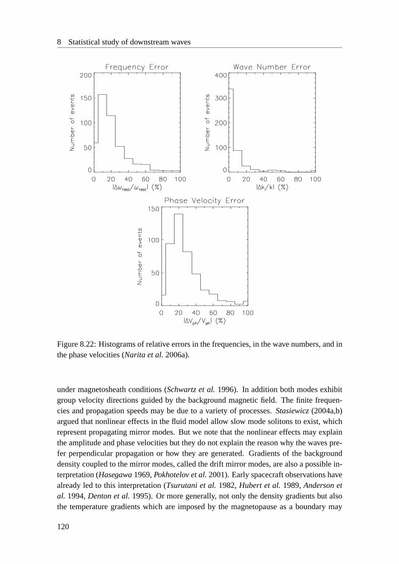
8 Statistical study of downstream waves
Figure 8.22: Histograms of relative errors in the frequencies, in the wave numbers, and inthe phase velocities (Narita et al.2006a).
under magnetosheath conditions (Schwartz et al.1996). In addition both modes exhibitgroup velocity directions guided by the background magnetic field. The finite frequen-cies and propagation speeds may be due to a variety of processes.Stasiewicz(2004a,b)argued that nonlinear effects in the fluid model allow slow mode solitons to exist, whichrepresent propagating mirror modes. But we note that the nonlinear effects may explainthe amplitude and phase velocities but they do not explain the reason why the waves pre-fer perpendicular propagation or how they are generated. Gradients of the backgrounddensity coupled to the mirror modes, called the drift mirror modes, are also a possible in-terpretation (Hasegawa1969,Pokhotelov et al.2001). Early spacecraft observations havealready led to this interpretation (Tsurutani et al.1982,Hubert et al.1989,Anderson etal. 1994,Denton et al.1995). Or more generally, not only the density gradients but alsothe temperature gradients which are imposed by the magnetopause as a boundary may
120

8.5 Summary
be coupled to the mirror modes so that they acquire a finite frequency by means of dia-magnetic drift effect, asJohnson and Cheng(1997) present the idea of the global mirrormodes in the magnetosheath. Identifying the excitation and propagation mechanism ofthe magnetosheath waves is an interesting problem, and the multi-point measurements ofCluster would be helpful for solving it, for example, investigating the dispersion curvesand group velocities, and comparing the rest frame frequencies with the drift mirror modefrequency or the diamagnetic drift frequency.
We also find that the wave propagation is away from the shock in both the upstreamand the downstream regions.Matsuoka et al.(2000) andSchafer et al.(2005) derivedthat the propagation sense in the magnetosheath is anti-sunward and outward in the samedirection as the plasma flow for the Alfvenic fluctuations of the magnetic field. The resultsconfirm their conclusion and in addition indicate that it is toward the magnetopause in themagnetosheath flank.Song et al.(1994) present that the waves are phase standing inthe flow near the magnetopause and therefore have a phase velocity oriented toward theshock in the plasma rest frame.Omidi and Winske(1995) interpret that such waves arethe mirror modes that pile up at the magnetopause boundary, but the study does not derivethe magnetosheath waves propagating toward the shock. Perhaps such waves are foundso close to the magnetopause that the event selection procedure does not count them.
We do not obtain clear signals for the ion cyclotron waves that may also be expectedto appear in the magnetosheath. Although the phase velocities detected are of the order ofthe intermediate mode speed, they are also of the same order as the slow mode speed andfurthermore the propagation angles are predominantly in the perpendicular direction to thebackground magnetic field. There is no clear difference in the magnetosheath between thequasi-parallel and the quasi-perpendicular shock regime for most of wave properties suchas frequencies, wave numbers and so on, but the phase angleφNB is not clear in the outerand the middle magnetosheath in the quasi-perpendicular shock regime.
Krauss-Varban and Omidi(1991, 1993) presented numerical simulations on the wavesupstream and downstream of the quasi-parallel shock and showed that the upstream fastmode waves are mode converted into the downstream ion cyclotron waves across theshock, while the wave vectors are oriented toward upstream in both cases. But the resultsshow that the wave vectors are oriented in the opposite direction to their conclusion inthe downstream region. The wave properties are not succeeded or transmitted from theupstream region to the downstream region as they argue.
8.5 Summary
In this chapter we have addressed the question of what typical wave properties in theupstream and the downstream region of the terrestrial bow shock are, how these wavespropagate, and how their characteristics differ between the quasi-parallel and the quasi-perpendicular shock regimes. The data used for the analysis are magnetic field and plasmameasurements made on board the four Cluster spacecraft. Cross spectral analyses as well
121

8 Statistical study of downstream waves
as the wave telescope technique have been used to analyze the observed wave activity. Asthe analysis allows to determine the Doppler shift, all results have been presented in theplasma rest frame. As for most data intervals analyzed it is determined whether observa-tions are made in the quasi-parallel or the quasi-perpendicular regime. An approximateclassification was made by introducing a special solar wind coordinate system which pro-vides a fast classification based on the ACE solar wind and magnetic field data. As weare also interested in knowing whether wave properties depend on where in the magne-tosheath the waves are observed, their properties are classified according to observationsmade into the upstream region, the outer, the middle, and the inner magnetosheath.
Moving from the upstream region through the shock toward the magnetopause, propa-gation directions change from being parallel to perpendicular to the background magneticfield. In the quasi-parallel shock regime this change is accompanied by a change of thetransport ratios of the phase angles between the magnetic field and the density fluctuationsfrom in-phase variations to out-of-phase variations, that is the upstream waves exhibit thefast mode characteristics and the downstream waves the mirror or the slow mode char-acteristics. Phase velocities agree with the fast mode speed in the upstream region andthe slow mode speed in the downstream region, respectively. In the quasi-perpendicularshock regime the transport ratio does not show clear signals except for the out-of-phasevariation in the inner magnetosheath. But otherwise the both regimes exhibit similar prop-erties in frequency, wave number, phase velocity, propagation angle, and polarization inboth the upstream and the downstream region. In the magnetosheath there is no cleardifference in these properties among the outer, the middle, and the inner magnetosheath.
The spatial pattern of wave propagation directions indicates an interesting structure.Propagation is outward divergent in the upstream region, inward divergent in the magne-tosheath near the magnetopause nose, and inward convergent in the magnetosheath flank.The divergent pattern in the magnetosheath indicates that the waves propagate along theplasma stream lines, following the refraction of the plasma flow at the shock. The con-vergent pattern in the magnetosheath flank which is consistent with the perpendicularpropagation in the draped magnetic field.
We conclude that wave properties are different the upstream and downstream region,but they are similar between the quasi-parallel and the quasi-perpendicular shock regime,suggesting that the upstream waves are not transmitted to the downstream region acrossthe shock and that the downstream waves do not depend on the shock angle. Our resultsalso suggest that in the foreshock the ion beam instabilities are operating with dominantright-hand mode and possibly with less dominant left-hand and non-resonant mode beingexcited. Upstream of the quasi-perpendicular shock the wave properties are similar tothat of the foreshock waves, but further investigations are needed to identify the wavesmodes. Both slow mode and mirror mode interpretations are possible for the magne-tosheath waves. In any case the magnetosheath waves have finite frequencies and phasevelocities that could result from various effects such as nonlinear effects and inhomo-geneities.
122

8.5 Summary
Table 8.1: Time intervals used in the statistical study of the magnetosheath waves, ob-servation Configurations of the magnetosheath observations (near quasi-parallel or nearquasi-perpendicular shock regime; magneothsheath shell), and dominant frequencies inthe spacecraft frame taken from 4-s and 1-s data set. A, B and C used in the magne-tosheath shell stand for the outer, the middle, and the inner magnetosheath, respectively.
Interval shock shell fsc(low) fsc(high)
mHz mHz2002-02-03 / 06:00-06:35 q-para A 56.6 187.52002-02-03 / 07:10-07:45 q-para B 40.0 125.02002-02-03 / 08:25-09:00 q-para C 41.0 89.82002-02-04 / 08:00-08:35 q-perp A 77.1 191.42002-02-04 / 03:45-04:20 q-perp B 110.4 203.12002-02-04 / 01:40-02:15 q-perp C 10.7 238.32002-02-06 / 11:55-12:30 q-perp A 52.7 105.52002-02-06 / 10:30-11:05 q-perp B 34.2 179.72002-02-08 / 23:20-23:55 q-para A 43.9 191.42002-02-08 / 21:00-21:35 q-perp B 10.7 218.82002-02-08 / 18:30-19:05 q-perp C 35.2 136.72002-02-11 / 09:00-09:35 q-perp A 59.6 246.12002-02-11 / 06:30-07:05 q-perp B 42.0 195.32002-02-11 / 02:30-03:05 q-perp C 24.4 187.52002-02-12 / 16:30-17:05 q-para A 91.8 191.42002-02-12 / 18:30-19:05 q-para B 12.7 238.32002-02-12 / 20:30-21:05 q-para C 74.2 265.62002-02-13 / 13:30-14:05 q-perp B 27.3 191.42002-02-15 / 01:00-01:35 q-para A 42.0 140.62002-02-15 / 03:00-03:35 q-perp B 45.9 289.12002-02-15 / 04:30-05:05 q-perp C 50.8 175.82002-02-16 / 05:00-05:35 q-perp A 44.9 171.92002-02-16 / 02:30-03:05 q-para B 53.7 164.12002-02-16 / 00:00-00:35 q-para C 66.4 82.02002-02-18 / 07:00-07:35 q-perp A 74.2 175.82002-02-18 / 06:10-06:45 q-para B 95.7 156.22002-02-18 / 05:10-05:45 q-para C 66.4 238.32002-02-19 / 17:30-18:05 q-para A 41.0 171.92002-02-19 / 20:30-21:05 q-para B 60.5 265.62002-02-19 / 23:00-23:35 q-para C 83.0 296.9
123

8 Statistical study of downstream waves
2002-02-20 / 15:30-16:05 q-para A 83.0 242.22002-02-20 / 14:30-15:05 q-para B 36.1 39.12002-02-20 / 13:15-13:50 q-para C 34.2 144.52002-02-23 / 05:30-06:05 q-perp A 43.0 261.72002-02-23 / 02:00-02:35 q-para B 114.3 136.72002-02-22 / 23:00-23:35 q-perp C 48.8 210.92002-02-25 / 08:45-09:20 q-perp B 24.4 43.02002-02-25 / 08:00-08:35 q-perp C 39.1 242.22002-02-26 / 22:15-22:50 q-para A 72.3 121.12002-02-26 / 23:15-23:50 q-perp B 50.8 128.92002-02-27 / 00:15-00:50 q-para C 35.2 199.22002-02-27 / 23:00-23:35 q-para A 53.7 175.82002-02-27 / 19:30-20:05 q-perp B 34.2 261.72002-02-27 / 16:30-17:05 q-perp C 34.2 160.22002-03-01 / 09:00-09:35 q-perp A 66.4 218.82002-03-02 / 07:45-08:20 q-para A 36.1 175.82002-03-02 / 05:45-06:20 q-para B 28.3 281.22002-03-02 / 04:00-04:35 q-para C 10.7 187.52002-03-03 / 18:00-18:35 q-para A 51.8 269.52002-03-03 / 20:00-20:35 q-para B 53.7 293.02002-03-03 / 21:25-22:00 q-para C 14.6 62.52002-03-04 / 13:10-13:45 q-perp A 114.3 43.02002-03-04 / 11:40-12:15 q-perp B 46.9 269.52002-03-04 / 10:00-10:35 q-perp C 74.2 78.12002-03-06 / 02:15-02:50 q-para A 78.1 277.32002-03-06 / 03:15-03:50 q-para B 45.9 261.72002-03-09 / 09:55-10:30 q-para A 31.2 332.02002-03-09 / 08:30-09:05 q-perp B 102.5 222.72002-03-09 / 06:45-07:20 q-para C 70.3 293.02002-03-10 / 19:00-19:35 q-para A 66.4 183.62002-03-10 / 21:30-22:05 q-perp B 64.5 187.52002-03-10 / 23:20-23:55 q-perp C 43.0 230.52002-03-11 / 18:00-18:35 q-perp A 65.4 289.12002-03-11 / 16:00-16:35 q-perp B 75.2 199.22002-03-11 / 14:00-14:35 q-perp C 16.6 328.12002-03-13 / 05:45-06:20 q-para A 30.3 128.92002-03-13 / 07:15-07:50 q-perp B 37.1 132.82002-03-13 / 09:15-09:50 q-para C 52.7 207.0
124

8.5 Summary
2002-03-14 / 04:30-05:05 q-perp A 24.4 160.22002-03-14 / 03:00-03:35 q-perp B 22.5 265.62002-03-14 / 01:30-02:05 q-perp C 30.3 242.22002-03-16 / 10:45-11:20 q-para A 114.3 187.52002-03-16 / 08:45-09:20 q-perp B 59.6 136.72002-03-16 / 06:30-07:05 q-perp C 46.9 457.02002-03-18 / 16:35-17:10 q-perp A 10.7 50.82002-03-18 / 15:50-16:25 q-perp B 112.3 218.82002-03-18 / 15:05-15:40 q-perp C 31.2 250.02002-03-23 / 13:55-14:30 q-para A 65.4 101.62002-03-23 / 13:00-13:35 q-para B 12.7 261.72002-03-23 / 12:00-12:35 q-para C 72.3 156.22002-03-25 / 05:30-06:05 q-perp B 96.7 335.92002-03-25 / 06:40-07:15 q-perp C 50.8 398.42002-03-27 / 10:15-10:50 q-para A 63.5 125.02002-03-27 / 12:00-12:35 q-perp B 92.8 128.92002-03-30 / 17:40-18:15 q-para A 114.3 113.32002-03-30 / 16:00-16:35 q-para B 36.1 191.42002-03-30 / 13:45-14:20 q-para C 31.2 210.92002-04-02 / 02:40-03:15 q-para A 114.3 238.32002-04-02 / 01:40-02:15 q-para B 54.7 109.42002-04-02 / 00:30-01:05 q-perp C 43.0 328.12002-04-03 / 17:15-17:50 q-perp B 26.4 152.32002-04-03 / 18:40-19:15 q-para C 33.2 164.12002-04-04 / 15:30-16:05 q-para A 60.5 171.92002-04-04 / 12:30-13:05 q-para B 41.0 238.32002-04-04 / 10:30-11:05 q-para C 26.4 168.02002-04-05 / 20:25-21:00 q-perp A 47.9 269.52002-04-05 / 21:25-22:00 q-perp B 61.5 293.02002-04-05 / 22:25-23:00 q-perp C 57.6 210.92002-04-07 / 00:30-01:05 q-para A 49.8 257.82002-04-06 / 22:00-22:35 q-para B 112.3 195.32002-04-06 / 19:15-19:50 q-para C 39.1 199.22002-04-08 / 05:00-05:35 q-para A 41.0 335.92002-04-08 / 06:10-06:45 q-para B 37.1 175.82002-04-09 / 07:10-07:45 q-perp A 55.7 238.32002-04-09 / 06:15-06:50 q-para B 52.7 214.82002-04-09 / 05:10-05:45 q-para C 56.6 308.6
125

8 Statistical study of downstream waves
2002-04-10 / 17:45-18:20 q-para A 48.8 140.62002-04-10 / 20:00-20:35 q-para B 31.2 125.02002-04-10 / 22:10-22:45 q-para C 27.3 246.12002-04-13 / 03:00-03:35 q-para A 85.9 109.42002-04-13 / 04:45-05:20 q-para B 31.2 199.22002-04-13 / 06:10-06:45 q-para C 10.7 199.22002-04-14 / 00:00-00:35 q-para A 44.9 148.42002-04-13 / 22:00-22:35 q-para B 100.6 234.42002-04-13 / 20:15-20:50 q-perp C 58.6 199.22002-04-15 / 14:15-14:50 q-perp B 32.2 144.52002-04-15 / 15:40-16:15 q-perp C 25.4 433.62002-04-18 / 22:00-22:35 q-para B 101.6 105.52002-04-18 / 19:00-19:35 q-para C 107.4 39.12002-04-21 / 07:00-07:35 q-para B 21.5 101.62002-04-21 / 04:30-05:05 q-para C 38.1 121.12002-04-22 / 14:00-14:35 q-para B 16.6 39.12002-04-22 / 16:30-17:05 q-para C 111.3 132.82002-04-23 / 12:15-12:50 q-para A 47.9 195.32002-04-23 / 10:30-11:05 q-perp B 77.1 156.22002-04-23 / 08:45-09:20 q-para C 64.5 50.82002-04-24 / 18:10-18:45 q-perp A 10.7 277.32002-04-24 / 19:40-20:15 q-para B 10.7 261.72002-04-26 / 01:00-01:35 q-para C 60.5 234.42002-04-28 / 07:10-07:45 q-para A 39.1 183.62002-04-28 / 06:00-06:35 q-para B 72.3 242.22002-04-30 / 19:30-20:05 q-para A 114.3 113.32002-04-30 / 15:30-16:05 q-perp B 33.2 218.82002-04-30 / 13:30-14:05 q-para C 57.6 78.12002-05-03 / 06:30-07:05 q-para A 45.9 281.22002-05-03 / 04:00-04:35 q-para B 37.1 285.22002-05-03 / 02:00-02:35 q-para C 38.1 140.62002-05-05 / 10:30-11:05 q-para A 39.1 117.22002-05-05 / 09:00-09:35 q-para B 43.9 144.52002-05-05 / 07:30-08:05 q-para C 27.3 105.52002-05-06 / 21:00-21:35 q-para B 24.4 281.22002-05-06 / 23:15-23:50 q-perp C 15.6 105.52002-05-07 / 22:20-22:55 q-para A 78.1 160.22002-05-07 / 20:00-20:35 q-para B 104.5 156.2
126

8.5 Summary
2002-05-07 / 17:30-18:05 q-para C 47.9 66.42002-05-09 / 06:25-07:00 q-perp C 111.3 234.42002-05-10 / 07:15-07:50 q-perp A 35.2 269.52002-05-10 / 06:15-06:50 q-perp B 33.2 214.82002-05-10 / 05:00-05:35 q-perp C 45.9 97.72002-05-11 / 15:00-15:35 q-para B 38.1 222.72002-05-11 / 17:00-17:35 q-para C 11.7 199.22002-05-12 / 13:00-13:35 q-perp B 85.9 269.52002-05-12 / 12:00-12:35 q-perp C 18.6 50.82002-05-15 / 02:30-03:05 q-para A 31.2 171.92002-05-15 / 00:00-00:35 q-para B 60.5 210.92002-05-14 / 21:45-22:20 q-para C 23.4 125.02002-05-17 / 11:30-12:05 q-para A 110.4 144.52002-05-17 / 09:30-10:05 q-para B 97.7 269.52002-05-17 / 07:30-08:05 q-perp C 82.0 257.82002-05-20 / 02:00-02:35 q-para A 38.1 140.62002-05-19 / 23:20-23:55 q-para B 46.9 156.22002-05-19 / 20:30-21:05 q-perp C 25.4 78.12002-05-20 / 11:25-12:00 q-para A 103.5 121.12002-05-20 / 16:25-17:00 q-para B 29.3 257.82002-05-21 / 00:00-00:35 q-perp C 87.9 246.12002-05-22 / 08:00-08:35 q-para A 83.0 277.32002-05-22 / 03:25-04:00 q-para B 53.7 101.62002-05-21 / 23:00-23:35 q-perp C 35.2 39.12002-05-27 / 10:00-10:35 q-para B 54.7 335.92002-05-30 / 06:30-07:05 q-para B 42.0 117.22002-05-30 / 10:00-10:35 q-para C 53.7 156.22002-05-31 / 21:00-21:35 q-para C 40.0 257.82002-06-01 / 21:00-21:35 q-para B 43.0 195.32002-06-02 / 00:30-01:05 q-perp C 83.0 136.72002-06-03 / 16:00-16:35 q-para B 42.0 218.82002-06-02 / 23:20-23:55 q-perp C 30.3 152.32002-06-04 / 06:30-07:05 q-para C 76.2 214.82002-06-05 / 22:00-22:35 q-para B 56.6 261.72002-06-05 / 11:25-12:00 q-perp C 54.7 74.22002-06-06 / 09:25-10:00 q-para C 82.0 140.62002-06-08 / 10:00-10:35 q-para B 27.3 93.82002-06-08 / 02:00-02:35 q-para C 76.2 156.2
127

8 Statistical study of downstream waves
2002-06-09 / 00:00-00:35 q-para C 59.6 109.42002-06-10 / 07:25-08:00 q-para B 43.0 140.62002-06-10 / 03:25-04:00 q-para C 87.9 101.62002-06-11 / 02:00-02:35 q-para C 72.3 168.02002-06-13 / 05:25-06:00 q-para B 26.4 203.12002-06-12 / 19:00-19:35 q-para C 33.2 261.72002-06-13 / 16:00-16:35 q-para C 43.0 179.72002-06-15 / 15:25-16:00 q-para B 53.7 250.02002-06-15 / 00:00-00:35 q-para C 53.7 113.32002-06-15 / 23:20-23:55 q-para C 111.3 132.82002-06-17 / 18:00-18:35 q-perp B 43.9 144.52002-06-17 / 10:00-10:35 q-perp C 54.7 168.0
128

8.5 Summary
Table 8.2: Time intervals and dominant frequencies taken from 4-s and 1-s magnetic fielddata used in the statistical study of the quasi-perpendicular shock upstream waves .
Interval fsc(low) fsc(high)
mHz mHz2002-02-03 / 00:00-00:35 99.6 453.12002-02-03 / 02:30-03:05 56.6 253.92002-02-04 / 09:00-09:35 36.1 97.72002-02-11 / 16:00-16:35 47.9 222.72002-02-11 / 18:00-18:35 14.6 320.32002-02-11 / 20:00-20.35 86.9 265.62002-02-12 / 04:00-04:35 60.5 296.92002-02-12 / 06:00-06:35 40.0 320.32002-02-12 / 08:00-08:35 42.0 312.52002-02-13 / 22:00-22:35 49.8 97.72002-02-16 / 09:00-09:35 37.1 253.92002-02-21 / 00:00-00:35 42.0 97.72002-02-21 / 07:00-07:35 33.2 273.42002-02-21 / 08:00-08:35 60.5 171.92002-02-21 / 20:00-20:35 56.6 265.62002-03-07 / 06:00-06:35 55.7 269.52002-04-23 / 15:30-16:05 52.7 308.62002-04-23 / 17:30-18:05 88.9 343.82002-04-24 / 17:00-17:35 43.9 97.7
129


9 Magnetic turbulence
9.1 Introduction
As the dispersion analyses have shown in Chapter 4, 5, and 7, waves are superposed overdifferent frequencies and wave numbers. The existence of waves with various frequenciesand wave numbers prefers the concept of turbulence. Turbulence is ubiquitous. It can beseen by gently stirring cream into coffee, or by observing wave caps at the beach, andit causes the drag on cars and aeroplanes. It is believed that the phenomenon is alsowidespread in magnetized plasmas.
As presented in Chapter 2, turbulence is often described as a process in which largescale eddies cascade down to smaller scale eddies until a scale is reached on which dis-sipation sets in. In magnetized plasmas it is not clear how the cascade progresses to thedissipation range, since there are a variety of possible small scale wave modes. Under-standing these processes would enable us to determine how energy flows in a turbulentplasma from large scales to the smaller, kinetic scale and thus heats the ambient plasma.
Turbulence in space plasma has been most extensively studied in the solar wind, butthe power spectra of the magnetic or velocity field fluctuations could be investigated onlyin the frequency domain, since the spacecraft have made one- or at best two-point mea-surements (Scarf et al.1981,Mellott 1986,Moustaizis et al.1986,Clasßen et al.1999,Bavassano Cattaneo et al.2000,Borovsky et al.2003). Earlier observations have alreadyshown that power spectra of the magnetic or velocity fields often contained an inertialrange with a slope of approximately -5/3 (Coleman1966, 1967, 1968), and also differentslopes depending on frequency scale: -1/3, -1, and -5/3 (Goldstein and Roberts1999).These observations could not distinguish clearly between a -5/3 and a -3/2 slope, as theyare close to each other. Here the -5/3 slope reflects the inertial range spectrum predictedby Kolmogorov(1941) for ideal, isotropic incompressible hydrodynamic turbulence, andthe -3/2 slope reflects the one predicted byKraichnan (1965) for ideal,incompressiblemagnetohydrodynamic turbulence. However, various case studies seem to indicate thatthe spectral slope is more often -5/3 (Marsch and Tu1990,Leamon et al.1998) in the fre-quency domain, although the solar wind fluctuations display anisotropic and compressiblefeatures.
It is not too surprising, as on the distance of 1 AU there is sufficient time for theturbulence to evolve into stationarity. This is not anymore the case when the solar winddevelops into shock waves which happens near planetary bow shocks, coronal mass ejec-
131

9 Magnetic turbulence
tions, and corotating interaction regions. The best accessible of all those shocks is theEarth’s bow shock which evolves in the super-Alfvenic (Mach numberMA ∼ 8 − 10)solar wind stream when it encounters the dipolar geomagnetic field. The presence of thesupercritical collisionless bow shock distorts the upstream plasma by reflecting a sub-stantial part of the solar wind plasma back into the solar wind along the interplanetarymagnetic field. Interaction between the two oppositely directed plasma streams causesvarious instabilities leading to the formation of the foreshock in front of the quasi-parallelbow shock, a highly non-quiescent region of wave excitation, damping, and wave particleinteractions as shown in Chapter 4, 5, and 6.
This raises the question whether or not the foreshock reaches a quasi-stationary tur-bulent state, which can best be answered by determining the turbulent wave number spec-trumP (k). This chapter attempts to determine the turbulence spectra in the wave numberdomain for the magnetic field fluctuation in the foreshock. The interval is 0805 - 0840UT on February 18, 2002, when inter-spacecraft separation was approximately 100 km.The time interval analyzed in this chapter is the same as that marked as “FS” in Fig. 6.1.
9.2 Dispersion curves andk-spectra
Determination of wave vectors consists in a search for the highest reliable wave powerpeaks ink-space for a given frequency interval. As the wave telescope provides a waveenergy distribution in thek-space, it is possible to identify multiple wave vectors con-tributing and their associated powers. The magnetic fluctuations measured by Cluster arein the frequency range0.02 < ωsc/2π < 2 Hz, when Cluster was in the foreshock of thequasi-parallel bow shock (ωsc is the frequency in the spacecraft frame). The accessiblewave number range is10−4 ≤ |k| < 10−1 km−1. We identify the basic wave modes fromthe experimentally determined dispersion relationω(k) = ωsc − k · vf , with vf the bulkflow velocity which in the present case was330± 30 km s−1.
The results are shown in Figs. 9.1, 9.3, and 9.4. The plasma frame dispersion relationof foreshock low-frequency waves as function ofω(|k|) is plotted in the upper panelof Fig. 9.1. Indicated are the proton cyclotron frequencyΩp = 1.1 rad s−1, the ion-inertial wave numberkin = ωp/c ≈ 1.3 × 10⁻² km−1, and the thermal ion gyroradiuswave numberkgy = Ωp/vth ≈ 7.3 × 10⁻³ km−1. Hereωp is the ion plasma frequencyΩp the ion cyclotron frequency,c the speed of light, andvth the ion thermal velocity.Each measurement point is given including error bars. We use the following grid sizefor scanning ink-space: |∆k| = 1.3 × 10⁻⁴ km−1 for |k| ≤ 1.0 × 10⁻² km−1, and|∆k| = 4.0× 10⁻⁴ km−1 for |k| > 1.0× 10⁻² km−1. The relative errors in wave numberare about 1.3%. The accuracy of the frequency in the plasma frame is determined bythe Doppler shift, i.e.|∆ω/ω| ≤ |∆k/k| + |∆vf/vf |. Relative errors of the velocityare∼14%, yielding|∆ω/ω| ∼15%. For the wave power we estimate the confidencelevel (Jenkins and Watts1968). The spatial sample power spectral estimator is essentiallya squared spectral estimate with aχ2 distribution, assuming that the sample amplitude
132

9.2 Dispersion curves andk-spectra
Figure 9.1: Wave frequency in the plasma frame showing (top) and wave power (bottom)as a function of wave number with error estimate. The symbolΩp denotes the protoncyclotron frequency. The wave power confidence on the 95% is also given (vertical errorbars in the bottom panel) Region A, B, and C represent the energy injection, the inertial,and the dissipation range, respectively. The symbolskin andkgy denote the ion inertialwave number and the thermal ion gyroradius wave number, respectively.
distribution is normal. Sixty-four degrees of freedom have been used.
The dispersion relation in Fig. 9.1 exhibits at least two branches shown in red andblue. For small|k| the blue branch starts at frequency close to zero bending upwardin frequency with increasing|k|. The red branch starts at a negative frequency of∼−0.7 rad s−1 before turning up logarithmically (ω ∼ ln k) and intersecting the blue branchclose to wave number|k| ∼ 2 × 10⁻³ km−1. Negative frequencies imply that the longwavelength waves propagate in the downstream direction. Closer inspection suggests thatnear intersection of the two branches the blue branch splits and connects to the red branch,indicating wave coupling in region A where the wave power (second panel) maximizes,probably leading to instability which injects energy into turbulence. From wave measure-ments alone it is not possible to decide what the energy source is as both branches gain in
133

9 Magnetic turbulence
power. The most probable source is provided by the shock-reflected ion beam present up-stream of the bow shock. Low frequency right-hand polarized whistler waves upstream ofthe collisionless shock are excited by a right-hand ion-ion beam instability (Gary 1991)and propagate along the background magnetic field. In addition a beam resonant wavepropagates along with the ion beam upstream into the solar wind. Dispersion analyseshave confirmed that the blue and red branches can approximately be identified with thesetwo wave modes, respectively (Chapter 4).
Toward larger wave numbers away from the energy injection region A the wave powerof the whistler branch (second panel) decreases in region B until the cut-off of the spec-trum in region C. This decay of the spectrum is described by a power law and thus indi-cates the existence of a turbulent quasi-inertial range inP (k) ∝ kα, with α = −1.9, ofroughly one order of magnitude extension in|k|. The third panel shows the formation of aplateau on the spectrum when the spectral decay is compensated by the above power lawfactor. The cut-off of the spectrum observed in region C is due to entering the dissipationrange. The boundary of this range is close to the gyro- and inertial wave numbers sug-gesting that gyro-viscosity/cyclotron damping limits the further extension of the inertialrange. The beam branch cannot be followed to larger wave numbers. Forming the upperfrequency branch of the dispersion relation at wave numbers above injection it ceases toexist even though it also exhibits a narrow quasi-inertial range of slopeα = −2.0, whichis slightly steeper than that of the dominant whistler branch, where most of the availablewave energy accumulates. The fact that the spectral slopes are close to -2 indicates inter-mittency which implies a breakdown of scaling law or self-similarity in the inertial rangecharacterized by a fluctuating energy transfer ratio.
Fig. 9.2 compares our directly determined|k|-spectrum with that obtained under Tay-lor’s hypothesis assuming that all the spatial structures are convected by the backgroundflow, and the temporal fluctuations reflect simply the spatial fluctuations. This assump-tion, of course, cannot be justified under the existence of waves that have certain prop-agation speeds. Even though both spectra are similar they exhibit distinct differences inshape and structure. The main spectral peaks are disparate by a factor of∼ 2 in |k|,and the direct spectrum is considerably steeper than the Taylor spectrum. Agreement isreached only at very small|k| for the largest turbulent eddies. Finally, the extension of theTaylor spectrum into very large|k| > (kgy, kin) is spurious as at such short wavelengthsmagnetic turbulence is well in the dissipation range where Taylor’s hypothesis fails. Wethus conclude that in the foreshock at all wavelengths of interest with the exception ofvery large eddies the turbulent state is not adequately described by the temporal spectraunder Taylor’s hypothesis.
We estimate the ratior = Rm,in/Rm,d of magnetic injection and dissipation regionReynolds numbers for the whistler branch assuming that the magnetic viscosity is con-stant. The wave energy ratio is about102, and the injection to dissipation scale ratio isabout12, yielding r ≈ 8.7 × 10⁴, using Eqs. (4.45) and (5.25) inBiskamp(2003). TheReynolds numbers at injection scales are thus very high.
134

9.2 Dispersion curves andk-spectra
Figure 9.2: Comparison ofk-spectra between the direct measurement using the wavetelescope and the indirect measurement using Taylor’s hypothesis.
Anisotropy
It is of interest to investigate anisotropy of the turbulence distinguishing between com-pressive,P‖(k⊥) ∝ 〈|B‖|2〉, and non-compressiveP⊥(k‖) ∝ 〈|B⊥|2〉 contributions to thepowerP (k). From∇ ·B = 0 these are given by
P‖,⊥ =P
1 + tan±2 θ, (9.1)
whereθ is the angle betweenk and the ambient magnetic field. Figs. 9.3 and 9.4 showthe respective dispersion relations and spectra for the non-compressive and compressivemodes. Note that the uncertainty increases in both cases since the number of data pointsis reduced.
The dispersion relation of the non-compressive mode (Fig. 9.3) exhibits the couplingbetween the two parallel propagating modes at the gap on the dispersion relation aroundk‖ ≈ 2 × 10⁻³ km−1 which splits the original wave branches. The two small-k‖ and thetwo large-k‖ beam and whistler branches seem to merge to form new dispersion branches,and the intensity on the beam mode maximizes. However, energy injection and iner-tial ranges are less well indicated in the wave power spectrum. The lower wave numberwhistler branch still exhibits a narrow quasi-inertial range belowk‖ ∼ 3 × 10⁻³ km−1.The higher wave number branch is, however, disparate and a quasi-inertial range can-not be identified. The spectrum exhibits a drop in power almost precisely at 0.5kgy
and possibly another one at 2kgy. The former may be related to gyro-resonant absorp-tion of wave energy by the plasma at the corresponding wave numbers. The absorbing
135
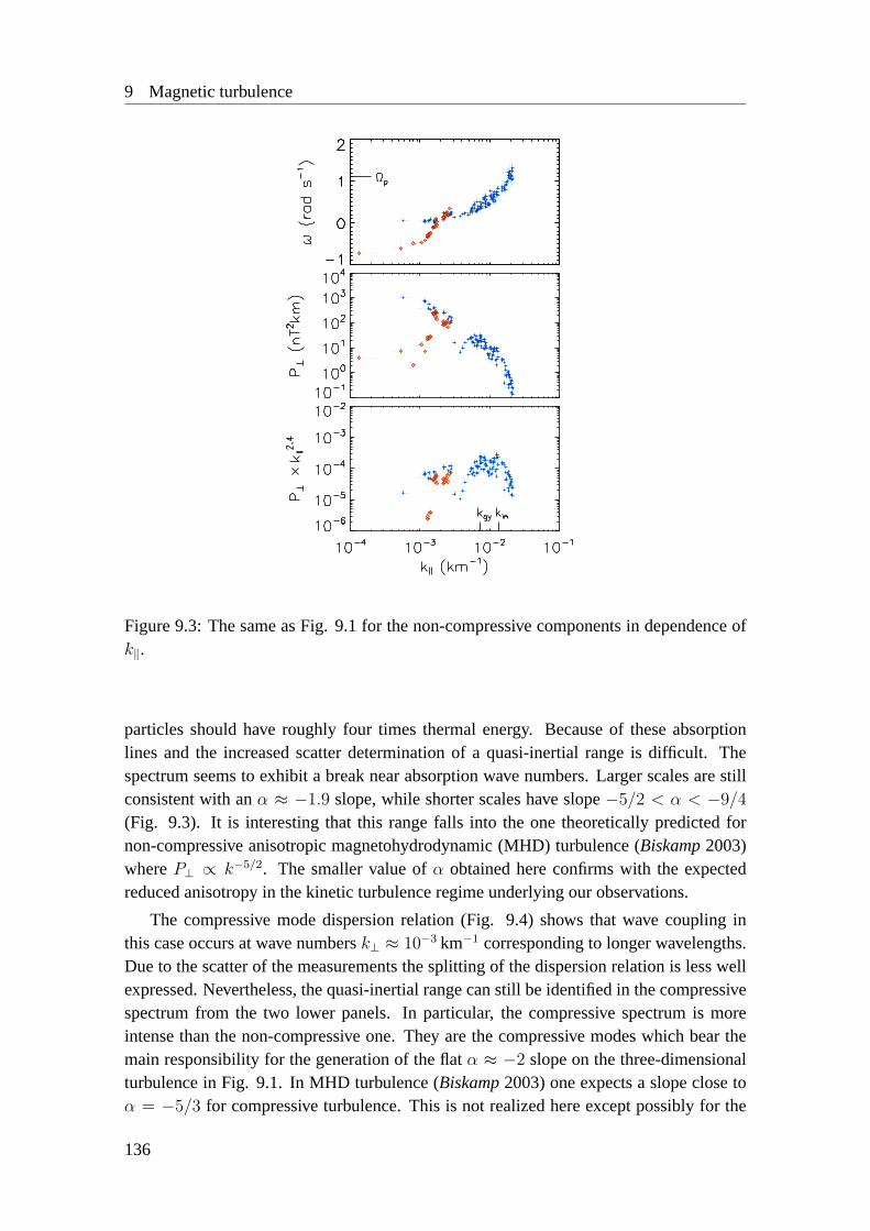
9 Magnetic turbulence
Figure 9.3: The same as Fig. 9.1 for the non-compressive components in dependence ofk‖.
particles should have roughly four times thermal energy. Because of these absorptionlines and the increased scatter determination of a quasi-inertial range is difficult. Thespectrum seems to exhibit a break near absorption wave numbers. Larger scales are stillconsistent with anα ≈ −1.9 slope, while shorter scales have slope−5/2 < α < −9/4
(Fig. 9.3). It is interesting that this range falls into the one theoretically predicted fornon-compressive anisotropic magnetohydrodynamic (MHD) turbulence (Biskamp2003)whereP⊥ ∝ k−5/2. The smaller value ofα obtained here confirms with the expectedreduced anisotropy in the kinetic turbulence regime underlying our observations.
The compressive mode dispersion relation (Fig. 9.4) shows that wave coupling inthis case occurs at wave numbersk⊥ ≈ 10−3 km−1 corresponding to longer wavelengths.Due to the scatter of the measurements the splitting of the dispersion relation is less wellexpressed. Nevertheless, the quasi-inertial range can still be identified in the compressivespectrum from the two lower panels. In particular, the compressive spectrum is moreintense than the non-compressive one. They are the compressive modes which bear themain responsibility for the generation of the flatα ≈ −2 slope on the three-dimensionalturbulence in Fig. 9.1. In MHD turbulence (Biskamp2003) one expects a slope close toα = −5/3 for compressive turbulence. This is not realized here except possibly for the
136

9.3 Discussion
Figure 9.4: The same as Fig. 9.1 for the compressive components in dependence ofk⊥.Note that the non-compressive intensity is one order of magnitude less than the compres-sive one.
short range of the red part of the spectrum, if taken separately.
9.3 Discussion
Turbulence in the foreshock consists of the general solar wind turbulence and superim-posed resonant wave modes excited in the foreshock boundary by the interaction betweenthe solar wind and intense streams of bow shock reflected particles. The wave modesreach large amplitudes depending on how long they stay in resonance along the fore-shock boundary. Entering the foreshock by convection with the solar wind toward thebow shock, they run out of resonance, start interacting with other waves, steepen to formnonlinear structures the long-wavelength part of which participates in shock reformation,while the shorter wavelengths enter the turbulent cascade. In the latter case the relationbetween frequencyω and wavenumberk looses its meaning of a linear dispersion relationdetermining one single wave mode. Whether or not an inertial range develops dependson the time the wave energy has to cascade down from injection to dissipation scales. Inthe bounded foreshock region this time is relatively short not allowing for the develop-
137

9 Magnetic turbulence
Figure 9.5: Probability distribution function (PDF) of the magnetic fields for the com-pressive part (δB‖) and the non-compressive part (δB⊥), plotted on the normalized (tothe Gaussian half-width) fluctuation amplitude. Solid curves in gray and in black repre-sent PDF superposed for four s/c data and PDF averaged over four s/c data, respectively.Dashed curves are Gaussian-fittings aroundδB = 0.
ment of stationary turbulence. One expects the turbulence to be in an intermittent state,not fully developed state exhibiting a true inertial range. The actual spectral slope shouldbe steeper than Kolmogorov’s inertial range slope withα = 5
3or Kraichnan’s slope with
α = 32. This is reflected in the observed spectral indicesα ≈ −1.9 for the dominant com-
pressive andα > −52
for the non-compressive turbulent spectra which indicate that theturbulence is intermittent possessing a still developing forward cascading quasi-inertialshort wavelength range. Thus, in addition to (nonlinear) wave modes, the foreshockcontains a substantial level of turbulence which is in an evolutionary intermittent state.Intermittency is also indicated by the bump on the end of this quasi-inertial range visibleon the compressive spectrum. Turbulent energy is accumulating at the scalek⊥ < kgy
just before entering the dissipative range. If the foreshock would be spatially more ex-tended, flattening of the spectrum should proceed from here backward until equilibriumwould be reached, possibly in the Kolmogorov states. In addition, further evidence forforeshock turbulence being intermittent is provided by the shapes of the probability distri-bution functions (PDFs) of the magnetic fluctuations shown in Fig. 3. These PDFs exhibitwell expressed non-Gaussian wings at large-fluctuation amplitudes and asymmetries inboth the compressive and non-compressive components for all four spacecraft typical forintermittency.
138
9.4 Summary
9.4 Summary
The direct experimental determination ofk-spectra of magnetic turbulence in the high-β
plasma upstream of a collisionless shock has been presented. The high-time resolutionmeasurements have been taken with Cluster at spacecraft separation of∼100 km. Thespectra exhibit three dynamnic ranges: an energy injection range atk ∼ 10−3 km−1, aquasi-inertial range10−3 < k < 10−2 km−1, and an indication of the dissipation rangek > 10−2 km−1. Dissipation starts close to the gyro-wave number suggesting that ion-viscosity is the main dissipative process. Compressive turbulence dominates the spectrumwith slopeα ≈ −1.9 suggesting intermittent non-stationary turbulence.
139


10 Summary and outlook
Measurements and observations made by the four Cluster spacecraft have been analyzedin pursuing low frequency wave characteristics upstream and downstream of the terrestrialbow shock. Shock waves are known to be found in many places in the Universe and to playan important role in accelerating cosmic ray particles. Studying the Earth’s bow shock isof significant importance, for it allows us to achieve detailed in-situ observations whoseresults have immediate astrophysical implications. The concept of the collisionless shockshave been presented in Chapter 2 together with reviews of the upstream and downstreamwaves, and turbulence. An overview of the Cluster spacecraft mission and reviews of theprinciples of magnetic field measurements and particle measurements has been presentedin Chapter 3. The methods of wave analyses using single and multi-point measurementshave been given in Chapter 3, too. The wave telescope technique has been extensivelyused and allowed not only to calculate wave powers associated with frequencies and wavenumbers but also to determine phase velocities, rest frame frequencies, dispersion curves,propagation patterns, and turbulence spectra.
Chapter 4 has presented the dispersion analysis of the upstream waves. The wavedispersion relation was determined experimentally and showed a good agreement withthe one calculated for the ion beam plasma model, suggesting that the upstream wavesrepresent a whistler and a beam resonant wave. This is one of the examples of wave modeidentification and confirms the physical processes drawn by the earlier studies that someupstream ions are specularly reflected at the shock and flow against the incoming ions,while they form an unstable particle distribution in velocity space which drives waves andcollapses into a stable state.
Chapter 5 has presented an example of wave-particle interaction. The dispersion andpolarization analysis indicated the existence of the whistler wave in the upstream region.The wave was accompanied by nongyrotropic electrons which were trapped by the wavefield. While it is known that some beam ions are phase bunched by the wave field, thereis also an interplay between the waves and the electrons.
Chapter 6 has presented the statistical study of the upstream waves. It was shown thatthe wave phase velocities in the plasma rest frame were oriented toward upstream alongthe magnetic field. This direction is the same as that of the backstreaming ions.
Chapter 7 has presented the dispersion analysis of the downstream waves. The dis-persion curves were investigated along a Cluster orbit and showed a transition from thewhistler and the beam resonant wave in the upstream region to the mirror mode in the
141

10 Summary and outlook
downstream region. The upstream waves are not transmitted across the shock, as they areswept by the solar wind toward downstream.
Chapter 8 has presented the statistical study of the downstream waves. While theupstream waves propagated parallel to the background magnetic field, the downstreamwaves propagated perpendicular. The mirror mode properties were frequently detectedin the downstream region but they had finite propagation speeds, possibly coupled to thebackground inhomogeneities. In the statistical average there is an organization in wavepropagation pattern: outward divergent in the upstream region; toward the magnetosheathflank region aligned with the plasma flow direction in the downstream region; and inwardconvergent in the magnetosheath flank.
Chapter 9 has attempted to determine the spectra of magnetic turbulence directly inthe wave number domain, showing three ranges appearing in the classical turbulence pic-ture: energy injection, inertial, and dissipation range. The inertial range spectrum was notthe classical Kolmogorov type or the Kraichnan type with the slope -5/3 and -3/2, respec-tively, but it showed an almost -2 slope, indicating that the fluctuations are intermittentand not fully developed turbulence. It was also understood on what scales the waves dampand thermalize the ambient plasma. Magnetic viscosity dominates on scale close to theion inertial length or the thermal ion gyroradius.
The disturbance in the plasma caused by the bow shock leads to wave excitation bothin the upstream and the downstream regions. The studies given in this thesis suggest thatultimately ion reflection is the cause of wave excitation in both regions, but as the waveproperties are different between them, the physical processes are accordingly different.The upstream waves propagate parallel to the magnetic field and are identified as the onedriven by the ion beam instability, while the downstream waves propagate perpendicu-lar and represent the mirror modes, possibly coupled to the background inhomogeneities.On the other hand they exhibit a unique propagation pattern imposed by the backgroundmagnetic field topology in those regions. Investigating spatial scales is essential in spaceplasma research. Dispersion relations and propagation patterns shown in the thesis maybe associated with planetary bow shocks, interplanetary shocks, and also shocks on astro-physical scales.
The thesis has attempted to answer a number of questions on waves and turbulence inspace, but it has raised on the other hand subjects that are left as open questions. They aresummarized as an outlook below.
(1) Are the upstream waves mode-converted at the shock? It was understood in Chap-ter 7 that the upstream waves (foreshock waves) were not transmitted into the downstreamregion. Are the waves mode-converted into different kinds of waves across the shock, orare they simply lost? In the latter case, into what energy the upstream wave energy ischanged?
(2) Why were the ion cyclotron waves not clearly detected? Neither the dispersionanalysis nor the statistical study showed a clear indication of the ion cyclotron waves. Theion cyclotron waves have a larger growth rate for temperature anisotropy instabilities, butobservationally the mirror modes dominate in the magnetosheath. Is it simply because
142

10 Summary and outlook
the former prefers a low value of plasma parameterβ, while the latter prefers a highβ?Since developed mirror modes exhibit magnetic bottle structures whereβ may be locallylow, it could be possible to detect the ion cyclotron waves in the magnetosheath.
(3) Is there any dependence on the Mach number orβ about the upstream and down-stream waves? It is known that the dynamics and the structure of a collisionless shockdepend not only on the shock angles (between the upstream magnetic field and the shocknormal) but also the Mach numbers andβ. In the statistical study wave properties were in-vestigated with respect to the shock angle for the quasi-parallel and the quasi-perpendicularshock regimes, but no clear difference was found. However, we do not know yet if waveexcitation, modes, and propagation speeds and directions depend on these two parameters.
(4) Technically, the spacecraft separation determines the largest wave number avail-able in the wave telescope analysis. In the case of Cluster one has at best 100 km sep-aration, which is roughly a typical scale of ion dynamics (thermal gyroradius or inertiallength) in the solar wind and in the magnetosheath. This means that the electron scale(less than 10 km) can not be resolved by Cluster, although its importance can be widelyacknowledged (e.g. Chapter 5). Future multi-spacecraft missions like MMS (Magneto-spheric Multi-Scale mission) will enable us to access the electron scale physics.
(5) It was presented that the turbulence spectra can be determined directly in the wavenumber domain. The wave number spectra shall be investigated in various regimes ofspace plasma: in the undisturbed solar wind and in the magnetosheath, where it is thoughtthat the Alfven and the mirror mode turbulence may exist.
(6) The mode recognition method (Glassmeier et al.1995), that is to identify energycontributions from the fast mode, intermediate mode, and slow mode waves, shall beapplied to the waves in the shock upstream and downstream regions.
(7) Of course, all the methods presented in the thesis can be applied to other regions ofthe magnetosphere. For instance, waves in the magnetotail or in the current sheets wouldbe an interesting subject. Dispersion curves and propagation patterns of the substorm-related waves shall be determined in future. The THEMIS mission (Time History ofEvents and Macroscale Interactions during Substorms) will answer fundamental questionsregarding the magnetospheric substorm instability.
In analyzing waves from in-situ observations in space, I conclude the PhD thesis bysaying that multi-point measurements are not only a powerful means but also an essen-tial means. Future multi-spacecraft missions are promising to better understand physicalprocesses of waves, instabilities, and turbulence in the collisionless plasma.
143


Bibliography
Anderson, B. J., S. A. Fuselier, S. A., and D. Murr, Electromagnetic ion cyclotron wavesobserved in the plasma depletion layer,Geophys. Res. Lett., 18, 1955-1958, 1991.
Anderson, B. J., S. A. Fuselier, S. P. Gary, and R. E. Denton, Magnetic spectral signaturesin the Earth’s magnetosheath and plasma depletion layer,J. Geophys. Res., 99, 5877-5891, 1994.
Arthur, C. W., R. L. McPherron, and J. D. Means, A comparative study of three techniquesfor using the spectral matrix in wave analysis,Radio Sci., 11, 833-845, 1976.
Asbridge, J. R, S. J. Bame, and I. B. Stron, Outward flow of protons from the Earth’s bowshock,J. Geophys. Res., 73, 5777-5782, 1968.
Balikhin, M. A., T. D. de Wit, H. S. C. K. Alleyne, L. J. C. Woolliscroft, S. N. Walker,V. Krasnosel’skikh, W. A. C. Mier-Jedrzejeowicz, and W. Baumjohann, Experimentaldetermination of the dispersion of waves observed upstream of a quasi-perpendicularshock,Geophys. Res. Lett., 24, 787-790, 1997a.
Balikhin, M. A., L. J. C. Woolliscroft, H. St. C. Alleyne, M. Dunlop, and M. A. Gedalin,Determination of the dispersion of low frequency waves downstream of a quasiperpen-dicular collisionless shock,Ann. Geophysicae, 15,143-151, 1997b.
Balikhin, M. A., S. Schwartz, S. N. Walker, H. St. C. K. Alleyne, M. Dunlop, and H. Luhr,Dual-spacecraft observations of standing waves in the magnetosheath,J. Geophys. Res.,106, 25,395-408, 2001.
Balogh, A., M. W. Dunlop, S. W. H. Cowley, D. J. Southwood, et al., The Cluster magneticfield investigation,Space Sci. Rev., 79, 65-91, 1997.
Balogh, A., Carr, C.M., Acuna, M.H., Dunlop, M.W., T. J. Beek, P. Brown, K.-H.Fornacon, E. Georgescu, K.-H. Glassmeier, J. Harris, G. Musmann, T. Oddy, K.Schwingenschuh, The Cluster magnetic field investigation: overview of in-flight per-formance and initial results,Ann. Geophysicae, 19, 1207-1217, 2001.
Barnes, A., Theory of generation of bow-shock-associated hydromagnetic waves in theupstream interplanetary medium,Cosmic Electrodyn., 1, 90-114, 1970.
145

Bibliography
Baumjohann, W., and R. A. Treumann,Basic space plasma physics, Imperial CollegePress, London, 1997.
Bavassano Cattaneo, M. B., G. Moreno, G. Russo, and J. D. Richardson, MHD turbulencein Saturn’s magnetosheath downstream of a quasi-parallel bow shock,J. Geophys. Res.,105, 23,141-152, 2000.
Bendat, J. S., and A. G. Piersol,Engineering applications of correlation and spectralanalysis, pp. 54-56, John Wiley & Sons, Inc., New York, 1980.
Biskamp, D., and H. Welter, Ion heating in high-Mach-number, oblique, collisionlessshock waves,Phys. Rev. Lett., 28, 410-413, 1972.
Biskamp, D., Magnetohydrodynamic Turbulence, Cambridge University Press, Cam-bridge, 2003.
Born, M. and E. Wolf,Principles of optics, 6th ed., pp. 503-504, 550, Pergamon press,New York, 1980.
Borovsky, J. E., and H. O. Funsten, MHD turbulence in the Earth’s plasma sheet: dynam-ics, dissipation, and driving,J. Geophys. Res., 108, 1284, doi:10.1029/2002JA09625,2003.
Burgess, D., Collisionless shocks,Introduction to space physics, (Eds) M. G. Kivelsonand C. T. Russell, pp. 129-163, Cambridge University Press, United Kingdom, 1995.
Burgess, D., What do we really know about upstream waves?,Adv. Space Res., 20, 673-682, 1997.
Cairns, I. H., D. H. Fairfield, R. R. Anderson, V. E. H. Carlton, K. I. Paularena, and A.J. Lazarus, Unusual location of Earth’s bow shock on September 24-25, 1987: Machnumber effects,J. Geophys. Res., 100, 47-62, 1995.
Claßen, H.-T, G. Mann, R. J. Forsyth, and E. Keppler, Low frequency plasma turbulenceand high energy particles at CIR-related shock waves,Astron. Astrophys., 347, 313-320, 1999.
Coleman, P. J., Hydromagnetic waves in the interplanetary plasma,Phys. Rev. Lett., 17,207-211, 1966.
Coleman, P. J., Wave-like phenomena in the interplanetary plasma: Mariner 2,Planet.Space Sci., 15, 953, 1967.
Coleman, P. J., Turbulence, viscosity, and dissipation in the solar-wind plasma,Astrophys.J., 153, 371, 1968.
146

Bibliography
Denton, R. E., S. P. Gary, X. Li, B. J. Anderson, J. W. Labelle, and M. Lessard, Low-frequency fluctuations in the magnetosheath near the magnetopause,J. Geophys. Res.,100, 5665-5679, 1995.
Denton, R. E., M. R. Lessard, J. W. Labelle, and S. P. Gary, Identification of low-frequency magnetosheath waves,J. Geophys. Res., 103, 23,661-676, 1998.
Dudok de Wit, T., V. V. Krasnosel’skikh, S. D. Bale, M. W. Dunlop, H. Luhr, S. J.Schwartz, and L. J. C. Woolliscroft, Determination of dispersion relations in quasi-stationary plasma turbulence using dual satellite data,Geophys. Res. Lett., 22,2653-2656, 1995.
Dubinin, E., K. Sauer, and J. F. McKenzie, Nonlinear stationary waves and solitons in ionbeam-plasma configuration,J. Geophys. Res., 109, A02208, 2004.
Eastwood, J. P., A. Balogh, M. W. Dunlop, T. S. Horbury, and I. Dandouras, Clusterobservations of fast magnetosonic waves in the terrestrial foreshock,Geophys. Res.Lett., 29, 2046-2049, 2002.
Eastwood, J. P., A. Balogh, E. A. Lucek, C. Mazelle, and I. Dandouras, On the existenceof Alfv en waves in the terrestrial foreshock,Ann. Geophysicae, 21, 1457-1465, 2003.
Escoubet, C.P., M. Fehringer, and M. Goldstein, The Cluster mission,Ann. Geophysicae,19, 1197-1200, 2001.
Fairfield, D., Bow shock associated waves observed in the far upstream interplanetarymedium,J. Geophys. Res., 74, 3541-553, 1969.
Fairfield, D. H., Whistler waves observed upstream from collisionless shocks,J. Geophys.Res., 79, 1368-1378, 1974.
Farris, M. H., and C. T. Russell, Determining the standoff distance of the bow shock:Mach number dependence and use of models,J. Geophys. Res., 99, 17,681-689, 1994.
Farris, M. H., C. T. Russell, C. T., and M. F. Thomsen, Wave activity associated withthe low beta collisionless shock, inSolar wind sources of magnetospheric ultra-low-frequency waves, pp. 99, Geophysical Monograph 81, (Eds) M. J. Engrebretson, K.Takahashi and M. Scholer, Amer. Geophys. Union, 1994.
Farrugia, C. J., G. Gnavi, F. T. Gratton, H. Matsui, R. B. Torbert, R. P. Lepping, N,Oieroset, and R. P. Lin, Electromagnetic ion cyclotron waves in the subsolar regionunder normal dynamic pressure: Wind observations and theory,J. Geophys. Res., 109,A02202, 2004.
Fowler, R.A., B. J. Kotick, and R. D. Elliott, Polarization analysis of natural and artifi-cially induced geomagnetic micropulsations,J. Geophys. Res., 72, 2871-2883, 1967.
147

Bibliography
Frisch, U.,Turbulence: the legacy of A. N. Kolmogorov, Cambridge University Press,Cambridge, 1995.
Fuselier, S. A., Energetic magnetospheric protons in the plasma depletion layer,J. Geo-phys. Res., 97, 13,759-13,766, 1992.
Fuselier, S. A., M. F. Thomsen, S. P. Gary, S. J. Bame, C. T. Russell, and G. K. Parks, Thephase relationship between gyrophase-bunched ions and MHD-like waves,Geophys.Res. Lett., 13, 60-63, 1986.
Gary, S. P., J. T. Gosling, and D. W. Forslund, The electromagnetic ion beam instabilityupstream of the Earth’s bow shock,J. Geophys. Res., 86, 6691-6696, 1981.
Gary, S. P., Low-frequency waves in a high-beta collisionless plasma: polarization, com-pressibility and helicity,J. Plasma Phys., 35, 431-447, 1986.
Gary, S. P., Electromagnetic ion/ion instabilities and their consequences in space plasmas- A review,Space Sci. Rev, 56, 373-415, 1991.
Gary, S. P., The mirror and ion cyclotron anisotropy instabilities,J. Geophys. Res., 97,8519-8529, 1992.
Gary, S., Theory of space plasma microinstabilities.Cambridge; Cambridge Atmos.Space Science Series, 1993.
Gary, S. P., S. A. Fuselier, and B. J. Anderson, Ion anisotropy instabilities in the magne-tosheath,J. Geophys. Res., 98, 1481-1488, 1993.
Gary, S. P., and D. Winske, Simulations of ion cyclotron anisotropy instabilities in theterrestrial magnetosheath,J. Geophys. Res., 98, 9171-9179, 1993.
Gary, S. P., P. D. Convery, R. E. Denton, S. A. Fuselier, and B. J. Anderson, Proton andhelium cyclotron anisotropy instability thresholds in the magnetosheath,J. Geophys.Res., 99, 5915-5921, 1994a.
Gary, S. P., M. E. McKean, D. Winske, B. J. Anderson, R. E. Denton, and S. A. Fuselier,The proton cyclotron instability and the anisotropy/B inverse correlation,J. Geophys.Res., 99, 5903-5914, 1994b.
Gary, S. P, and M. A. Lee, The ion cyclotron anisotropy instability and the inverse corre-lation between proton anisotropy and proton beta,J. Geophys. Res., 99, 11,297-11,301,1994.
Gedalin, M., Yu. E. Lyubarsky, M. Balikhin, and C. T. Russell, Mirror modes: non-Maxwellian distributions,Phys. Plasmas, 8, 2934-2945, 2001.
148

Bibliography
Gedalin, M., M. Balikhin, R. J. Strangeway, and C. T. Russell, Long-wavelength mirrormodes in multispecies plasmas with arbitrary distributions,J. Geophys. Res., 107, A2,doi:10.1029/2001JA000178, 2002.
Glassmeier, K.-H., and U. Motschmann, Comments on time-series analysis,Proc. ofthe workshop on data analysis tools, (Eds) Glassmeier, K.H., Motschmann, U., andSchmidt, R., ESA SP-371, 7-14, ESA Publications Division, The Netherlands, 1995.
Glassmeier, K.-H., U. Motschmann, and R. v. Stein, Mode recognition of MHD wavefields at incomplete dispersion measurements,Ann. Geophysicae, 13, 76-83, 1995.
Glassmeier, K.-H., U. Motschmann, M. Dunlop, A. Balogh, M. H. Acuna, C. Carr, G.Musmann, K.-H. Fornacon, K. Schweda, J. Vogt, E. Georgescu, and S. Buchert, Clusteras a wave telescope - first results from the fluxgate magnetometer,Ann. Geophysicae,19, 1439-1447, 2001 (Correction,Ann. Geophysicae, 21, 1071, 2003).
Goldstein, M. L., and D. A. Roberts, Magnetohydrodynamic turbulence in the solar wind,Phys. Plasmas, 6, 4154-4160, 1999.
Gosling, J. T., J. R. Asbridge, S. J. Bame, G. Paschmann, and N. Sckopke, Observationsof two distinct populations of bow shock ions in the upstream solar wind,Geophys.Res. Lett., 5, 957-960, 1978.
Greenstadt, E. W., I. M. Green, G. T. Inouye, A. J. Hundhausen, S. J. Bame, and I. B.Strong, Correlated magnetic field and plasma observations of the Earth’s bow shock,J.Geophys. Res., 73, 51-60, 1968.
Gurgiolo, C., M. L. Goldstein, Y. Narita, K.-H. Glassmeier, and A. N. Fazakerley, A phaselocking mechanism for nongyrotropic electron distributions upstream of the Earth’sbow shock,J. Geophys. Res., 110, A06206, 2005.
Hasegawa, A., Drift mirror instability in the magnetosphere,Phys. Fluids, 12, 2642, 1969.
Hasegawa, A., and L. Chen, Theory of the drift mirror instability,Plasma waves andinstabilities at comets and in magnetospheres, pp. 173-177, Washington DC, Amer.Geophys. Union, Geophysical Monograph Series, 1989.
Hassam, A. B., Transmission of Alfven waves through the Earth’s bow shock: theory andobservation,J. Geophys. Res., 83, 643-653, 1978.
Hellinger, P., A. Mangeney, and A. Matthews, Whistler waves in 3D hybrid simulationsof quasiperpendicular shocks,Geophys. Res. Lett, 23, 621-624, 1996.
Hellinger, P., P. Travnıcek, and V. I. Sotnikov, Whistler waves in the foot region of per-pendicular shock: hybrid simulations,Proc. of 6th European Workshop on CollisionlessShock, pp. 29, 2005.
149

Bibliography
Hill, P., G. Paschmann, R. A. Treumann, W. Baumjohann, N. Sckopke, and H. Luhr,Plasma and magnetic field behavior across the magnetosheath near local noon,J. Geo-phys. Res., 100, 9575-9584, 1995.
Hoppe, M. M., C. T. Russell, L. A. Frank, T. E. Eastman, and E. W. Greenstadt, Upstreamhydromagnetic waves and their association with backstreaming ion populations - ISEE1 and 2 observations,J. Geophys. Res., 86, 4471-4492, 1981.
Hoppe, M. M., and C. T. Russell, Plasma rest frame frequencies and polarizations ofthe low-frequency upstream waves - ISEE 1 and 2 observations,J. Geophys. Res., 88,2021-2027, 1983.
Hubert, D., C. C. Harvey, and C. T. Russell, Observations of magnetohydrodynamicmodes in the earth’s magnetosheath at 0600 LT,J. Geophys. Res., 94, 17,305-309,1989.
Hubert, D., C. Lacombe, C. C. Harvey, M. Moncuquet, C. T. Russell, and M. F. Thomsen,Nature, properties, and origin of low-frequency waves from an oblique shock to theinner magnetosheath,J. Geophys. Res., 103, 26,783-26,798, 1998.
Iroshnikov, P. S., Turbulence of a conducting fluid in a strong magnetic field,Sov. Astron.,7, 566-571, 1964.
Jenkins, G. M., and D. G. Watts,Spectral analysis and its applications, pp. 313-317,Holden-Day, San Francisco, 1968.
Johnson, J. R., and C. Z. Cheng, Global structure of mirror modes in the magnetosheath,J. Geophys. Res., 102, 7179-7189, 1997.
Johnstone, A. D., and C. Alsop, and S. Burge, P. J. Carter, A. J. Coates, A. J. Coker, A.N. Fazakerley, N. Grande, R. A. Gowen, C. Gurgiolo, B. K. Hancock, B. Narheim,A. Preece, P. H. Sheather, J. D. Winningham, and R. D. Woodliffe, PEACE: a plasmaelectron and current experiment,Space Sci. Rev., 79, 351-398, 1997.
Kennel, C. F., J. P. Edmiston, and T. Hada, A quarter century of collisionless shock re-search, in Collisionless shocks in the heliosphere: a tutorial review,Geophys. Monogr.Ser., 34, (Eds) R. G. Stone and B. T. Tsurutani, pp. 1-36, Amer. Geophys. Union, Wash-ington, DC, 1985.
Kivelson, M. G., Pulsation and magnetohydrodynamic waves, inIntroduction to spacephysics, pp. 330-355, (Eds) M. G. Kivelson and C. T. Russell, Cambridge UniversityPress, 1995.
Kivelson, M. G., and D. J. Southwood, Mirror instability II: the mechanism of nonlinearsaturation,J. Geophys. Res., 101, 17,365-17,371, 1996.
150

Bibliography
Kolmogorov, A. N., The local structure of turbulence in incompressible viscous fluid forvery large Reynolds number,Dokl. Akad. Nauk SSSR, 30, 9-13, 1941 (reprinted inProc.R. Soc. Lond.A 434, 9-13, 1991).
Kraichnan, R. H., Inertial range spectrum in hydromagnetic turbulence,Phys. Fluids, 8,1385-1387, 1965.
Krall, N. A., What do we really know about collisionless shocks?,Adv. Space Res., 20,715-524, 1997.
Krasnosel’skikh, V., Nonlinear motions of a plasma across a magnetic field,Sov. Phys.Jetp., 62, 282, 1985.
Krasnosel’skikh, V. V., B. Lembege, P. Savoini, and V. V. Lobzin, Nonstationarity ofstrong collisionless quasiperpendicular shocks: theory and full particle numerical sim-ulations,Phys. Plasmas, 9, 1192-1209, 2002.
Krauss-Varban, D., and N. Omidi, Structure of medium Mach number quasi-parallelshocks - upstream and downstream waves,J. Geophys. Res., 96, 17,715-731, 1991.
Krauss-Varban, D., and N. Omidi, Propagation characteristics of waves upstream anddownstream of quasi-parallel shocks,Geophys. Res. Lett. 20, 1007-1010, 1993.
Krauss-Varban, D., Bow shock and magnetosheath simulations: wave transport and ki-netic properties,Solar wind sources of magnetospheric ultra-low-frequency waves, pp.121-134, Geophysical Monograph 81, Amer. Geophys. Union, 1994.
Krauss-Varban, D., N. Omidi, and K. B. Quest, Mode properties of low-frequency waves:kinetic theory versus Hall-MHD,J. Geophys. Res., 99, 5987-6009, 1994.
Leamon, R. J., C. W. Smith, N. F. Ness, and W. H. Matthaeus, Observational constraintson the dynamics of the interplanetary magnetic field dissipation range,J. Geophys.Res., 103, 4775-4787, 1998.
Marsch, E., and C.-Y. Tu, On the radial evolution of MHD turbulence in the inner helio-sphere,J. Geophys. Res., 95, 8211-8229, 1990.
Marsden, R. G., E. J. Smith, J. F. Cooper, and C. Tranquille, Ulysses at high heliographiclatitudes: an introduction,Astron. Astrophys., 316, 279, 1996.
Matsuoka, A., D. J. Southwood, S. Kokubun, and T. Mukai, Propagation sense of low-frequency MHD waves in the magnetosheath observed by Geotail,J. Geophys Res.,105, 18,361-376, 2000.
Matthaeus, W. H. and M. L. Goldstein, Measurement of the rugged invariants of magne-tohydrodynamic turbulence in the solar wind,J. Geophys. Res., 87, 6011-6028, 1982.
151

Bibliography
Matsukiyo, S., and M. Scholer, Modified two-stream instability in the foot of high Machnumber quasi-perpendicular shocks,J. Geophys. Res., 108, SMP 19-1, 2003.
Mazelle, C., D. Queeau, and K. Meziane, Nonlinear wave particle interactions due toquasi-monochromatic ULF waves in the Earth foreshock,Nonlinear Processes in Geo-phys., 7, 185-190, 2000.
McKenzie, J. F., and K. O. Westphal, Transmission of Alfven waves through the Earth’sbow shock,Planet. Space Sci., 17, 1029-1037, 1969.
McKenzie, J. F., and K. O. Westphal, Interaction of hydromagnetic waves with hydro-magnetic shocks,Phys. Fluids, 13, 630-640, 1970.
McPherron, R. L., Magnetospheric dynamics,Introduction to space physics, pp. 448,(Eds) M. G. Kivelson and C. T. Russell, Cambridge University Press, 1995.
Mellott, M. M., Plasma wave signatures of collisionless shocks and the role of plasmawave turbulence in shock formation,Adv. Space Res., 6, 25-32, 1986.
Merka, J., A. Szabo, A., T. W. Narock, J. H. King, K. I. Paularena, J. D. Richardson, Acomparison of IMP 8 observed bow shock positions with model predictions,J. Geo-phys. Res., 108, SMP6-1, CiteID 1077, doi:10.1029/2002JA009384, 2003.
Meziane, K., C. Mazelle, C. D’Uston, H. Reme, R. P. Lin, C. W. Carlson, D. Larson, J.P. McFadden, R. E. Ergun, K. A. Anderson, G. K. Parks, D. Berdichevsky, and R. P.Lepping, Wind observation of gyrating-like ion distributions and low frequency wavesupstream from the earth’s bow shock,Adv. Space Res., 20, 703-706, 1997.
Meziane, K., C. Mazelle, R. P. Lin, D. LeQueau, D. E. Larson, G. K. Parks, and R. P. Lep-ping, Three-dimensional observations of gyrating ion distributions far upstream fromthe Earth’s bow shock and their association with low-frequency waves,J. Geophys.Res., 106, 5731-5742, 2001.
Mobius, E., H. Kucharek, C. Mouikis, E. Georgescu, L. M. Kistler, M. A. Popecki, M.Scholer, J. M. Bosqued, H. Reme, C. W. Carlson, B. Klecker, A. Korth, G. K. Parks,J. C. Sauvaud, H. Balsiger, M.-B. Bavassano-Cattaneo, I. Dandouras, A. M. Dilellis,L. Eliasson, V. Formisano, T. Horbury, W. Lennartsson, R. Lundin, M. McCarthy, J.P. McFadden, and G. Paschmann, Observations of the spatial and temporal structure offield-aligned beam and gyrating ring distributions at the quasi-perpendicular bow shockwith Cluster CIS,Ann. Geophysicae, 19, 1411-1420, 2001.
Motschmann, U., T. I. Woodward, K.H. Glassmeier, and M. W. Dunlop, Array signal pro-cessing techniques,Proc. CLUSTER workshop on data analysis tools, pp. 79-86, (Eds)Glassmeier, K.H., Motschmann, U., and Schmidt, R., ESA SP-371, ESA PublicationsDivision, The Netherlands, 1995.
152

Bibliography
Motschmann, U., T. I. Woodward, K. H. Glassmeier, D. J. Southwood, and J.L. Pincon,Wavelength and direction filtering by magnetic measurements at satellite arrays: gen-eralized minimum variance analysis,J. Geophys. Res., 101, 4961-4965, 1996.
Moustaizis, S., D. Hubert, A. Mangeney, C. C. Harvey, C. Perche, and C. T. Russell,Magnetohydrodynamic turbulence in the Earth magnetosheath,Ann. Geophysicae, 4,355-362, 1986.
Narita, Y., K.-H. Glassmeier, S. Schafer, U. Motschmann, K. Sauer, I. Dandouras, K.-H. Fornacon, E. Georgescu, and H. Reme, Dispersion analysis of ULF waves in theforeshock using cluster data and the wave telescope technique,Geophys. Res. Lett., 30,SSC 43-1, 2003.
Narita, Y., K.-H. Glassmeier, S. Schafer, U. Motschmann, M. Franz, I. Dandouras, K.-H. Fornacon, E. Georgescu, A. Korth, H. Reme, and I. Richter, Alfven waves in theforeshock propagating upstream in the plasma rest frame: statistics from Cluster obser-vations,Ann. Geophysicae 22, 2315-2323, 2004.
Narita, Y., and K.-H. Glassmeier, Dispersion analysis of low-frequency waves throughthe terrestrial bow shock,J. Geophys. Res., 110, A12215, doi:10.1029/2005JA011256,2005.
Narita, Y. , K.-H. Glassmeier, K.-H. Fornacon, I. Richter, S. Schafer, U. Motschmann,I. Dandouras, H. Reme, and E. Georgescu, Low frequency wave characteristics in theupstream and downstream regime of the terrestrial bow shock,J. Geophys. Res., 111,A01203, doi:10.1029/2005JA011231, 2006a.
Narita, Y., K.-H. Glassmeier, and R. A. Treumann, Magnetic turbulence spectra in thehigh-beta plasma upstream of the terrestrial bow shock,Phys. Rev. Lett., submitted,2006b.
Narita, Y. and K.-H. Glassmeier, Low-frequency waves in the bow shock environment,Proc. of the Cluster and Double Star symposium - 5th anniversary of Cluster in space,(Ed) K. Fletcher, ESA SP-598, ESA Publications Division, The Netherlands, 2006.
Ness, N. F., C. S. Scearce, and J. B. Seek, Initial results of the IMP 1 magnetic fieldexperiment,J. Geophys. Res., 69, 3531, 1964.
Ogilvie, K. W., T. von Rosenvinge, and A. C. Durney, International Sun-Earth Explorer,a three spacecraft program,Science 198, 131-138, 1977.
Omidi, N., and D. Winske, Structure of the magnetopause inferred from one-dimensionalhybrid simulations,J. Geophys. Res., 100, 11,935-955, 1995.
Orlowski, D. S., C. T. Russell, and R. P. Lepping, Wave phenomena in the upstream regionof Saturn,J. Geophys. Res., 97, 19,187-199, 1992.
153

Bibliography
Orlowski, D. S., and C. T. Russell, Comparison of properties of upstream whistlers atdifferent planets,Adv. Space Res., 16, 137-141, 1995.
Paschmann, G., N. Sckopke, S. J. Bame, J. R. Asbridge, J. T. Gosling, C. T. Russell, andE. W. Greenstadt, Association of low-frequency waves with suprathermal ions in theupstream solar wind,Geophys. Res. Lett., 6, 209-212, 1979.
Paschmann, G., N. Sckopke, I. Papamastorakis, J. R. Asbridge, S. J. Bame, and J. T.Gosling, Characteristics of reflected and diffuse ions upstream from the Earth’s bowshock,J. Geophys. Res., 86, 4355-4364, 1981.
Paschmann, G., A. N. Fazakerley, and S. J. Schwartz, Moments of plasma velocity distri-butions,Analysis methods for multi-spacecraft data, pp. 125-158, (Eds) G. Paschmannand P. W. Daly, ISSI Scientific Report SR-001 (Electronic ed. 1.1), ISSI/ESA, 2000.
Pincon, J. L., and F. Lefeuvre, Local characterization of homogeneous turbulence in aspace plasma from simultaneous measurement of field components at several points inspace,J. Geophys. Res., 96, 1789-1802, 1991.
Pokhotelov, O. A., M. A. Balikhin, R. A. Treumann, and V. P. Pavlenko, Drift mirrorinstability revisited: 1. cold electron temperature limit,J. Geophys. Res., 106, 8455-8464, 2001.
Price, C. P., D. W. Swift, and L.-C. Lee, Numerical simulation of nonoscillatory mirrorwaves at the Earth’s magnetosheath,J. Geophys. Res., 91, 101-112, 1986.
Reiff, P. H., The use and misuse of statistical analysis, pp. 493-522,Solar-terrestrialphysics - fundamental principles, ed. R. L. Carovillano and J. M. Forbes, D. Reidel,Boston, MA, 1983.
Reme, H., C. Aoustin, J. M. Bosqued, I. Dandouras, B. Lavraud, J. A. Sauvaud, A. Barthe,J. Bouyssou, Th. Camus, O. Coeur-Joly, A. Cros, J. Cuvilo, F. Ducay, Y. Garbarowitz,J. L. Medale, E. Penou, H. Perrier, D. Romefort, J. Rouzaud, C. Vallat, D. Alcayde, C.Jacquey, C. Mazelle, C. D’Uston, E. Mobius, L. M. Kistler, K. Crocker, M. Granoff, C.Mouikis, M. Popecki, M. Vosbury, B. Klecker, D. Hovestadt, H. Kucharek, E. Kuen-neth, G. Paschmann, M. Scholer, N. Sckopke, E. Seidenschwang, C. W. Carlson, D. W.Curtis, C. Ingraham, R. P. Lin, J. P. McFadden, G. K. Parks, T. Phan, V. Formisano, E.Amata, M. B. Bavassano-Cattaneo, P. Baldetti, R. Bruno, G. Chionchio, A. di Lellis,M. F. Marcucci, G. Pallocchia, A. Korth, P. W. Daly, B. Graeve, H. Rosenbauer, V.Vasyliunas, M. McCarthy, M. Wilber, L. Eliasson, R. Lundin, S. Olsen, E. G. Shelley,S. Fuselier, A. G. Ghielmetti, W. Lennartsson, C. P. Escoubet, H. Balsiger, R. Friedel,J.-B. Cao, R. A. Kovrazhkin, I. Papamastorakis, R. Pellat, J. Scudder, and B. Son-nerup, First multispacecraft ion measurements in and near the Earth’s magnetospherewith the identical Cluster ion spectrometry (CIS) experiment,Ann. Geophysicae, 19,1303-1354, 2001.
154

Bibliography
Russell, C. T., D. D. Childers, and J. P. J. Coleman, OGO 5 observations of upstreamwaves in interplanetary medium: discrete wave packets,J. Geophys. Res., 76, 845-861,1971.
Russell, C.T., Planetary bow shocks,Collisionless shocks in the heliosphere: reviews ofcurrent research, Geophysical Monograph 35, (Eds) B.T. Tsurutani and R. G. Stone,pp.109, Amer. Geophys. Union, Washington, D.C., 1985.
Russell, C. T., Multipoint measurements of upstream waves,Adv. Space Res., 8, 147-156,1988.
Sauer, K., E. Dubinin, and J. F. McKenzie, New type of soliton in bi-ion plasmas andpossible implications,Geophys, Res. Lett., 28, 3589, 2001.
Sauer, K., and E. Dubinin, Oscillitons and gyrating ions in a beam-plasma system,Geo-phys, Res. Lett., 30, 2192, 2003.
Scarf, F. L., D. A. Gurnett, and W. S. Kurth, Plasma wave turbulence at planetary bowshocks,Nature, 292, 747-750, 1981.
Schafer, S., K.-H. Glassmeier, Y. Narita, K.-H. Fornacon, M. Franz, and I. Dandouras,Statistical phase propagation and dispersion analysis of low frequency waves in themagnetosheath,Ann. Geophysicae, 23, 3339-3349, 2005.
Scholer, M., and S. Matsukiyo, Nonstationarity of quasi-perpendicular shocks: a compar-ison of full particle simulations with different ion to electron mass ratio,Ann. Geophys-icae, 22, 2345-2353, 2003.
Schwartz, S. J., D. Burgess, and J. J. Moses, Low-frequency waves in the Earth’s magne-tosheath: present status,Ann. Geophysicae, 14, 1134-1150, 1996.
Schwartz, S. J., Shock and discontinuity normals, Mach numbers, and related parameters,Analysis methods for multi-spacecraft data, (Eds) G. Paschmann and P. W. Daly, ISSIScientific Report SR-001 (Electronic ed. 1.1), pp. 249-270, ISSI/ESA, 2000.
Sckopke, N., G. Paschmann, A. L. Brinca, C. W. Carlson, and H. Luhr, Ion thermalizationin quasi-perpendicular shocks involving reflected ions,J. Geophys. Res., 95, 6337-6352, 1990.
Shue, J.-H., J. K. Chao, H. C. Fu, C. T. Russell, P. Song, K. K. Khurana, and H. J. Singer,A new functional form to study the solar wind control of the magnetopause size andshape, shocks involving reflected ions,J. Geophys. Res., 102, 9497-9511, 1997.
Smith, C. W., H. K. Wong, and M. L. Goldstein, Whistler waves associated with theUranian bow shock - outbound observations,J. Geophys. Res., 96, 15,841-852, 1991.
155

Bibliography
Sonett, C. P., and I. J. Abrams, The distance geomagnetic field, 3, Disorder and shocks inthe magnetopause,J. Geophys. Res., 68, 1233, 1963.
Song, P., C. T. Russell, and S. P. Gary, Identification of low-frequency fluctuations in theterrestrial magnetosheath,J. Geophys. Res., 99, 6011-6025, 1994.
Sonnerup, B. U.O., and M. Scheible, Minimum and maximum variance analysis,Analysismethods for multi-spacecraft data, (Eds) G. Paschmann and P. W. Daly, ISSI ScientificReport SR-001 (Electronic ed. 1.1), pp. 185-220, ISSI/ESA, 2000.
Southwood, D. J., and M. G. Kivelson, Mirror instability: 1. physical mechanism of linearinstability,J. Geophys. Res., 98, 9181-9187, 1993.
Sreenivasan, K. R., On the universality of the Kolmogorov constant,Phys. Fluids, 7,2778-2784, 1995.
Stasiewicz, K., Reinterpretation of mirror modes as trains of slow magnetosonic solitons,Geophys. Res. Lett., 31, L21804, doi:10.1029/2004GL021282, 2004.
Stasiewicz, K., Theory and observations of slow-mode solitons in space plasmas,Phys.Rev. Lett., 93, 12, 2004.
Stasiewicz, K., Nonlinear Alfven, magnetosonic, sound, and electron inertial waves influid formalism,J. Geophys. Res., 110, A03220, doi:10.1029/2004JA010852, 2005.
Stix, T. H.,Waves in plasmas, pp. 10, Springer-Verlag, New York, 1992.
Stone, E. C., A. M. Frandsen, R. A. Mewaldt, E.R. Christian, D. Margolies, J.F. Ormes,and F. Snow, The Advanced Composition Explorer,Space Sci. Rev., 86, 1 - 22, 1998.
Thomsen, M. F., J. T. Gosling, S. J. Bame, and C. T. Russell, Gyrating ions and large-amplitude monochromatic MHD waves upstream of the Earth’s bow shock,. J. Geo-phys. Res., 90, 267, 1985.
Tidman, D. A., and T. G. Northrop, Emission of waves by the Earth’s bow shock,J.Geophys. Res., 73, 143, 1968.
Treumann, R. A., and W. Baumjohann,Advanced space plasma physics, pp. 341-352,Imperial College Press, London, 1997.
Treumann, R. A., and M. Scholer, The magnetosphere as a plasma laboratory,The Centuryof space science, 1495-1528, Kluwer Academic Publishers, The Netherlands, 2001.
Treumann, R. A., C. H. Joroschek, O. D. Constantinescu, R. Nakamura, O. A. Pokhotelov,and E. Georgescu, The strange physics of low frequency mirror mode turbulence in thehigh temperature plasma of the magnetosheath,Nonlinear Processes in Geophys., 11,647-657, 2004.
156

Bibliography
Tsurutani, B. T., E. J. Smith, R. R. Anderson, K. W. Ogilvie, J. D. Scudder, D. N. Baker,and S. J. Bame, Lion roars and nonoscillatory drift mirror waves in the magnetosheath,J. Geophys. Res., 87, 6060-6072, 1982.
Tu, C.-Y., and E. Marsch, MHD structures, waves, and turbulence in the solar wind:observations and theories,Space Sci. Rev., 73, 1-210, 1995.
Van Dyke, M.,An album of fluid motion., The Parabolic Press, Stanford, CA, 1982.
Velli, M., and F. Pruneti, Alfven waves in the solar corona and solar wind,Plasma phys.control. fusion, 39, B317-B324, 1997.
Verigin M. I., M. Tatrallyay, G. Erdos, and G. A. Kotova Magnetosheath - interplanetarymedium reference frame: application for a statistical study of mirror type waves in theterrestrial plasma environment,Adv. Space Res., 35in press, 2006.
Warhaft, Z., Turbulence in nature and in the laboratory,Proc. the National Acad. Sci., 99,2481-2486, 2002.
Wenzel, K.-P., R. G. Marsden, D. E. Page, and E. J. Smith, The Ulysses mission,Astron.Astrophys. Suppl., 92, 207, 1992.
Wong, H. K., and M. L. Goldstein, Proton beam generation of oblique whistler waves,J.Geophys. Res., 93, 4110-4114, 1988.
Wu, C. S., D. Winske, Y. M. Zhou, S. T. Tsai, P. Rodriguez, M. Tanaka, K. Papadopoulos,K. Akimoto, C. S. Lin, M. M. Leroy, and C. C. Goodrich, Microinstabilities associatedwith a high Mach number, perpendicular bow shock,Space Sci. Rev., 37, 63-109, 1984.
157


Acknowledgments
The author is most grateful to his advisor Prof. Dr. Karl-Heinz Glassmeier at the Institutfur Geophysik und extraterrestrische Physik (IGEP) in Braunschweig. Having a respectto both experiments and theories and keeping balance between them, there is much tolearn from the advisor. His support and respect in all situations were essential not only inpursuing this PhD thesis but also in growing as a scientist, never forcing any knowledgeor attitudes upon the author, but rather forcing himself to keep an open mind and lettingthe author develop his own ideas.
The author is also very grateful to IGEP colleagues: Dr. Alexander Bogdanov whowas a member of IGM (former IGEP) for granting the author of foundations about thewave analyses using magnetometer data as well as fruitful discussions and suggestions;Karl-Heinz Fornacon, Dr. Ingo Richter, and Dr. Hans-Ulrich Auster for calibrationof the Cluster FGM instruments and processing data as well as teaching the author theprinciples of fluxgate magnetometers. Dragos Constantinescu for wonderful discussionson physics; Sebastian Schafer for the implementation of the wave telescope program;IGEP ULF group (Constantinescu, Schafer, Kleindiest, and Schmidt) for discussing wavephysics and programming; Carsten Schmidt for improving the author’s German disputa-tion; Michael Rost and Kai Okrafka for assisting the author with understanding computerhardware/software; Sabine Filbrandt and Nicole Ringleb for kind assistance in coordinat-ing travel, finding financial sources, and processing administrations.
Prof. Dr. Uwe Motschmann at the Institut fur Theoretische Physik, Braunschweig,has also encouraged the author as well. Being a theoretician who pays attention to exper-imental physics as much as theoretical physics, his comments and questions are compactbut nevertheless very accurate and illuminating in pursuing physics. The author thanksfor an opportunity to share the authorship with him in the publications.
Prof. Dr. Rudolf Treumann at the Max-Planck-Institut fur extraterrestrische Physik(MPE), Garching, has paid a lot of attention and interest in this PhD thesis. During thediscussions on turbulence, he made every endeavor to bring the turbulence work into theworld and visited Braunschweig all the way from Munich many times. The author looksup for his attitudes in pursuing physics as well as his talented piano play and thanks to hisunselfish collaboration sincerely.
Dr. Gotz Paschmann at the International Space Science Institute (ISSI), Berne, Swiss,has coordinated to summarize a lot of Cluster results in the dayside magnetosphericboundaries in to an ISSI series book. The author thanks for his kind invitation to the
159

Acknowledgments
Figure 10.1: The first meeting of the scientists who proposed the magnetic field investi-gation on Cluster in November 1986 in TU Braunschweig. Standing, from the left, BruceTsurutani, Jim Slavin, Hermann Luhr, Andre Balogh, Gunter Musmann, Mario Acuna,David Southwood, Fritz Primdahl, Konrad Schwingenschuh, Alain Meyer, Alain Roux;sitting, Rick Elphic and Karl-Heinz Glassmeier.
ISSI book and providing a chance to see a lot of famous space physicists in Berne in2003, which was a wonderful experience.
Dr. Melvyn Goldstein at NASA Goddard Space Flight Center, USA, and Dr. ChrisGurgiolo at Bitterroot Basic Research, USA, have kindly conducted a collaboration be-tween the Cluster FGM and PEACE (electron) investigations that led to the publication(Gurgiolo et al.2005). The author thanks to them for their kind assistance in providingdata, discussing the analysis methods and the results.
This PhD thesis relies significantly on the measurements made by the Cluster FGMinvestigation. The author is very grateful to those who have been working for nearly twodecades to bring its concept into reality, especially to those who appear in Fig. 10.1.Also many thanks to Edita Georgescu at MPE for the FGM calibration, Prof. Dr. AndreBalogh, Dr. Elizabeth Lucek, Dr. Chris Carr, Dr. Patrick Brown, and Dr. Tim Oddy inthe Imperial College, London, and all members of the Cluster FGM team.
Prof. Dr. Henri Reme, Dr. Iannis Dandouras and Dr. Elsa Chretien at Centre d’EtudeSpatiale des Rayonnements (CESR), Toulouse, France assisted the author when using theion data obtained by the CIS instruments. The author is also grateful to those who havebeen working with CIS for providing ion data.
The author is also grateful to Dr. Andrew N. Fazakerley and his team for providingelectron data for granting a permission to use PEACE images for this thesis.
The author thanks to Dr. Philippe Escoubet at ESA for management of the Clustermission.
Dr. Norman F. Ness and Dr. David J. McComas have kindly provided the ACE MAGand ACE SWEPAM data for this PhD work. The author is grateful to them and theirrespective groups.
The author is grateful to Prof. Dr. C. R. O’Dell at Vanderbilt University, NASA, andESA for permitting to use the Hubble Space Telescope image.
The author is grateful to Dr. S. Peter Gary at the Los Alamos National Laboratory,
160

Acknowledgments
Unites States, for his comments and suggestions on turbulence.The author thanks deeply to Dr. Dieter Schmitt at the Max-Planck-Institut fur Son-
nensystemforschung (MPS) for his kind decision to adopt the author as a PhD studentfrom Japan and for his organization of the International Max-Planck Research School(IMPRS).
The author is obliged to Prof. Dr. Konrad Sauer at MPS for his kind collaboration inpublishing the paperNarita et al. (2003), and to Dr. Axel Korth as well as Dr. MarkusFranz for their kind assistance in the paperNarita et al.(2004).
This PhD thesis owes a lot to Dr. Masatoshi Yamauchi, Prof. Dr. Ingrid Sandahl, Prof.Dr. Rickard Lundin, Dr. Lars Eliasson, and all the colleagues at the Swedish Institute ofSpace Physics (IRF), Kiruna, Sweden, since an experience with the particle data of theAstrid-2 satellite in Kiruna in 1999 was very precious and inspiring for the author. Alsomany thanks to Dr. Olle Norberg at Esrange, Kiruna, who carried most of the Astrid-2project on his shoulders.
The author owes also a lot to Prof. Toshifumi Mukai and Prof. Kiyoshi Maezawaat Japan Aerospace Exploration Agency, Institute of Space and Astronautical Science(JAXA/ISAS) for their complete advising in the Master degree program given at GraduateSchool of Tokyo University. They suggested the author to challenge the PhD degree inBraunschweig and wrote immediately a successful recommendation letter to Germany.Without their advise the author would not know how meaningful it is to study physics inGermany. The author is also grateful for Prof. Dr. Atsuhiro Nishida at Japan Society forPromotion of Science for encouraging studying physics in Germany.
The author is obliged a lot to Prof. Dr. Ryoichi Fujii at Nagoya University for coordi-nating the author’s visit in Nagoya University and a seminar in 2004.
Remembering the days of physics courses given at Tokyo Metropolitan University in1996-2000, the author wishes to express his best gratitude to Prof. Dr. Satoru Saito for ev-erything he has taught, supported, encouraged. He is the one who inspired the author withthe courage to always challenge physics through all his lectures and unselfishly assistedthe author to challenge in Kiruna. Being not only an elementary particle physicist and afield theoretician but also a talented lecturer with very rich background experiences, hekept on giving a lively lecture and the author can not count how many first-year studentsat TMU were inspired by him in the right direction.
The author is also grateful to Prof. Dr. Takao Saito at Tohoku University, Japan, whoimmediately recommended IRF-Kiruna as a potential institute that would lead the authorin the right direction in studying space physics.
Also many thanks to Takuya Masunaga and Satoshi Iijima who studied physics andmathematics at TMU together with the author in 1996-1999. Their insight in science,physics, mathematics are outstanding and they encouraged the author to keep an openmind for everything in life.
Birger Liliergren in Kiruna has been kindly exchanging letters with the author sincethe author stayed in Kiruna in 1999. Communicating with him in Swedish was the onlyhope to guess some German words for the author to survive the first half year in Braun-
161

Acknowledgments
schweig.Finally, the author thanks very much to his wife Maki, his parents Kazue and Haruhito,
and big brother Norihito for supporting the author in many many situations.
162
Curriculum Vitae
Personal Details:
Name: Yasuhito NaritaDate of Birth: November 13, 1977Place of Birth: Nagoya, Aichi Prefecture, JapanNationality: JapaneseMarital Status: Married with Maki NaritaParents: Haruhito Narita (father) and Kazue Narita (mother)
Current Activity:
Staff scientist at Institute for Geophysics andextraterrestrial Physics, Technical University of Braunschweig since 2002
Universities and Institutes:
M.Sc. Space Physics at University of Tokyo 2002Graduate School of Science, University of Tokyo/Institute of Space and Astronautical Science, Sagamihara 2000-2002B.Sc. Physics at Tokyo Metropolitan Univesity 2000Swedish Institute of Space Physics, Kiruna, Sweden 1999Tokyo Metropolitan University 1996-2000
School Education:
Asahigaoka Senior High School, Aichi 1993-1996Sakurada Junior High School, Nagoya 1990-1993Kasugano Elementary School, Nagoya 1983-1990
163

Curriculum Vitae
Publications:
Yasuhito Narita, Plasma domain observed by ASTRID-2, IRF Scientific Report 265, ISSN0284-1703, Kiruna, Sweden, March 2000.
Hφymork, S. H., M. Yamauchi, Y. Ebihara, Y. Narita, O. Norberg und D. Winningham,Dense ion clouds of 0.1 - 2 keV ions inside the CPS-region observed by Astrid-2,Ann.Geophysicae, 19, 621-631, 2001.
Schafer, S., K.-H. Glassmeier, Y. Narita, K.-H. Fornacon, I. Dandouras und M. Franz,Statistical phase propagation and dispersion analysis of low frequency waves in themagnetosheath,Ann. Geophysicae, 23, 3339-3349, 2005.
164