low frequency electromagnetic investigation of
TRANSCRIPT

The Pennsylvania State University
The Graduate School
College of Engineering
LOW FREQUENCY ELECTROMAGNETIC INVESTIGATION OF
FRACTURES AND RESERVOIRS USING PROPPANTS
A Dissertation in
Electrical Engineering
by
Muhammed K. Hassan
© 2014 Muhammed K. Hassan
Submitted in Partial Fulfillment
of the Requirements
for the Degree of
Doctor of Philosophy
August 2014

The dissertation of Muhammed K. Hassan was reviewed and approved* by the following: Raj Mittra Professor of Electrical Engineering Dissertation Adviser Co-Chair of Committee James K. Breakall Professor of Electrical Engineering Co-Chair of Committee Michael T. Lanagan Professor of Engineering Science and Mechanics Lynn A. Carpenter Emeritus Associate Professor of Electrical Engineering Kultegin Aydin Professor of Electrical Engineering Head of the Department of Electrical Engineering *Signatures are on file in the Graduate School

iii
ABSTRACT
An electromagnetic method is developed to analyze materials at different
frequencies by modeling the materials as equivalent dipoles. This method enabled us to
understand the scattering behavior of materials. The formulation of this new approach,
which is based on the Dipole Moment Method, is useful for solving electromagnetic
scattering problems at low frequencies and in finding the scattered fields of the scattering
object at any given distance from the object. By replacing scatterers with their equivalent
dipole moment weight, the method can be used to analyze a wide variety of materials,
including magneto-dielectric materials. This approach is first investigated using simple
geometries. Following this simple and useful method, the method was extended to the
study of multiple scattering objects. The dipole weights for these objects can be obtained
using either the near field or the far field approach. More complex and realistic bodies
and three-dimensional problems can be solved by using this new electromagnetic method.
Once the materials have been modeled, the developed technique is then compared
with effective medium theories, to decide which one can use to choose a mixing rule. For
the case of complex reservoirs and large fractures, one can easily use the effective
medium theory formulations, and the results do not show much difference, which serves
as a validation to the dipole moment method. A low-frequency Finite Element Method
was implemented to handle forward modeling of fractures with magnetic permeability
contrasts that can be created by injecting fluids with magnetic proppants. The Finite
Element Method is found to handle complex geometries and overcomes the limitations of
the Finite Difference Time Domain Method at low frequencies, as is needed to

iv
investigate deep fractures. The depth of the fractures was correlated with the scattered
fields. Given the measured value of the fields scattered by a given fracture, we can
estimate the depth of the fracture. The research enhanced our understanding of fracture
propagation and sensing with magnetic proppants using electromagnetic waves, which is
very important in enhancing resource recovery and evaluating reserves.

v
TABLE OF CONTENTS
LIST OF FIGURES ..................................................................................................... vii
ACKNOWLEDGEMENTS ......................................................................................... x
Chapter 1 Introduction ................................................................................................ 1
1.2 Methods for Fracture Characterization ........................................................... 4 1.3 Scope of Research Work ................................................................................ 6
Chapter 2 Low-Frequency Method for Scattering from a Single Object by using the Dipole Moment Technique ............................................................................. 10
2.1 Introduction ..................................................................................................... 10 2.2 Motivation ....................................................................................................... 11 2.3 Concept of the DM Technique ....................................................................... 12 2.4 Dipole Moment (DM) Technique: Near-Field Method .................................. 14
2.4.1 Numerical Results ................................................................................ 15 2.4.2 Observations ......................................................................................... 20
2.5 Dipole Moment Technique: Far-Field Patterns Method ................................. 21 2.5.1 Mathematical Proof of Method ............................................................ 21 2.5.2 Electric Fields Radiated by X-, Y-, Z- Oriented Dipole Moments ...... 23 2.5.3 Numerical Results ................................................................................ 25
2.6 Conclusions ..................................................................................................... 29
Chapter 3 Multiple Scattering using the Dipole Moment Approach ........................... 30
3.1 Introduction ............................................................................................................ 30
3.2 Dipole-Moment Formulation for Multiple-Scattering Objects .............................. 30 3.2.1 Modeling Using Spheres ............................................................................... 31 3.2.2 Consistency Factor Computation .................................................................. 31 3.3 Dipole Moment–MOM Formulation ..................................................................... 33
3.3.1 Examples of Magneto Dielectric Random Spherical Particles Scattering Problems ......................................................................................................... 35
3.4 Monte Carlo Techniques ........................................................................................ 38 3.5 Conclusion ............................................................................................................. 49
Chapter 4 Mixing Rules and Materials Properties for Proppants ............................... 50
4.1 Introduction ..................................................................................................... 50 4.2 Properties of Proppants and Their Slurry ....................................................... 51

vi
4.3 Retrieval of Permeability and Permittivity Of Materials Using Transmission/Reflection Methods ................................................................. 53
4.4 Effective Medium Theory ............................................................................... 56 4.4.1 Mixtures with Spherical Inclusions ...................................................... 57 4.4.2 Interaction of Particles in Mixture ........................................................ 59 4.4.3 Other Mixing Formulas ........................................................................ 60 4.5 Unified Mixing Rule ................................................................................ 62
4.6 Conclusion ...................................................................................................... 66
Chapter 5 Analysis of Fractures ................................................................................... 68
5.1 Introduction ..................................................................................................... 68 5.2 Fields of Magnetic Dipole in Uniform Conducting Medium ......................... 68 5.3 Effect of Magnetic Permeability on Fractures ................................................ 76 5.3 Magnetic Dipole in Two-Layer Permeability Materials ................................. 78 5.4 Analysis of Response of Instruments in Presence of Fractures ...................... 86 5.5 Numerical Method for Analysis of Complex Fractures ................................. 90
5.5.1 Finite Element formulation for Fractured Shale Medium .................... 92 5.6 Conclusions ..................................................................................................... 100
Chapter 6 Conclusions and Recommendations for Further Research ........................ 102
6.1 Conclusions ................................................................................................... 102 6.2 Recommendation for Future Work ................................................................. 103
Bibliography.................................................................................................................105

vii
LIST OF FIGURES
Figure 1-1 Source: U.S. Energy Information Administration, Annual Energy Outlook 2014, May 7, 2014. ................................................................................. 2
Figure 2-1: PEC sphere illuminated with X-polarized, Z-directed incident electric field ....................................................................................................................... 15
Figure 2-2: Amplitude comparison of back scattered field with distance along z-axis ........................................................................................................................ 16
Figure 2-3: Amplitude variation with frequency comparison at a point λ/100 ........... 17
Figure 2-4: PEC cylinder ............................................................................................ 17
Figure 2-5: Amplitude variation with distance along z-axis for PEC cylinder .......... 18
Figure 2-6: Variation of Ex with frequency at observation point for PEC cylinder ... 18
Figure 2-7: PEC cube .................................................................................................. 19
Figure 2-8: Variation of Ex with distance z-axis for a cube ....................................... 19
Figure 2-9: Variation of Ex with frequency at observation point 9 mm along z-axis for a cube ....................................................................................................... 20
Figure 2-10: PEC sphere illuminated with X-polarized, Z-directed incident electric field .......................................................................................................... 25
Figure 2-11: Amplitude comparison of back-scattered field with distance along z-axis ........................................................................................................................ 26
Figure 2-12: Variation of Ex with frequency at observation point for PEC sphere ... 27
Figure 2-13: PEC cone ................................................................................................ 27
Figure 2-14: Variation of Ex with frequency at observation point for PEC cone ...... 28
Fig 2-15: PEC cone cylinder ....................................................................................... 28
Figure 2-16: Variation of Ex with frequency at observation point 9 mm along z-axis for the cylinder .............................................................................................. 29

viii
Figure 3-1: Scattering from 14 randomly distributed spherical particles ................... 36
Figure 3-2: Validation of DM with FDTD: scattered electric Field (Ez) on a line .... 37
Figure 3-3: Discrete random distribution of particles in a 1-meter cube box ............. 42
Figure 3-4: Incident field set up for the simulation .................................................... 43
Figure 3-5: Graph showing the mean of the ensemble realizations and individual realizations ............................................................................................................ 44
Figure 3-6: Variance of ensemble realizations ........................................................... 44
Figure 3-7: Standard Deviation of the realizations ..................................................... 45
Figure 3-8: Plot shows a linear relationship between the volume of particles in different cube sizes and scattered electric fields. .................................................. 46
Figure 3-9: The depths of the cuboid were D(m)=[0.3, 0.45, 0.65, .75, 0.9, 1] ......... 47
Figure 3-10: Plot of Scattered Electric Fields vs. Varying Depth with fixed Width .. 48
Figure3-11: Relationship of Maximum Scattered Electric Field with varying Depth ..................................................................................................................... 48
Figure 4-1 Susceptibility of Material vs. Volume in a Mixture .................................. 53
Figure 4-2: Ratio of Susceptibility of Mixture in Maxwell Garnett Formula. ........... 59
Figure 4-3: Effect of Volume on Low-Permeability Materials for Different Mixing Rules ........................................................................................................ 63
Figure 4-4: Effect of Volume of inclusions on High-Permeability Materials for Different Mixing Rules ......................................................................................... 64
Figure 4-5: Plot Comparing Scattered Fields from Mixing Rules and DM Approach. .............................................................................................................. 65
Figure 4.6: Variation of Effective Medium of Materials with Volume and Permeability for Bruggeman Mixing Formula. .................................................... 66
Figure 5-1: Two-Coil Instrument in Conducting Medium ......................................... 71
Figure 5-2. Effect of Permeability on Magnetic Field on a Permeable Sphere (r=9cm). ................................................................................................................ 77
ix
Figure 5-3: Two-Layer Medium with Transmitter and Receivers .............................. 78
Figure 5-4: Fracture cross section showing probes and induced currents. ................. 86
Figure 5-6: Hydraulic fractured well arrangement showing shale, with cross section of horizontal well with a vertical fracture. ............................................... 99
Figure 5-7: Relationship between scattered Magnetic fields and fracture depths for a given fracture geometry ............................................................................... 99
Figure 5-8: Scattered electric fields due to fractures of different lengths .................. 100

x
ACKNOWLEDGEMENTS
This thesis could never have come together without the help of many people.
Firstly, I sincerely thank my advisor, Dr. Raj Mittra, who always gave me the gentle push
I needed to continue my work despite the constant wave of discouraging results. I would
also like to thank Prof. James Breakall, Mike Lanagan, and Lynn Carpenter for their
encouragement, for agreeing to serve on my committee, and for reviewing this
dissertation.
I am grateful to all my fellow Electromagnetic Communication Lab students and
scholars, especially Kadappan and Mohamed, for their help during my years at Penn
State. My special thanks to my friends, Melvin Eze and William Broewer, for
encouragement and for making me believe that achieving the goals of my work is
possible.
I am grateful to my wife, Zainab, for her love and support and to my Mum and
Dad for instilling courage in me and for their prayers for my success. I acknowledge the
Petroleum Technology Development Fund for funding part of this PhD and my family for
additional financial support.

1
Chapter 1
Introduction
Hydraulic fracturing is an increasingly useful method for the recovery of gas from
shale reservoirs. Shale reservoirs generally have low permeability but good porosity to
trap hydrocarbons in geologic formations. The low permeability of the reservoirs makes
recovery of the hydrocarbons difficult. In the hydraulic fracturing technique, forcing
high-pressured fluid with proppants into a horizontal well to break shale reservoirs
creates fractures. This fracturing process increases the permeability of the reservoirs and
creates new pathways to allow gas to flow. The rise of this technique is significant in
increasing the natural gas production in the USA [1]. Four major developments
contributing to the increase in production are: 1) the use of fluids for fracturing; 2) the
ability to drill horizontal wells longer than 5000 feet; 3) the ability to create a network of
multiple fractures in stages of about 10-20 per horizontal well; and 4) being able to create
the fractures simultaneously or sequentially during the drilling operation. Fracturing is
also useful for enhanced oil recovery from complex hydrocarbon reservoirs as well as for
geothermal energy recovery and the recovery of other resources. The fractures created
during drilling serve as pathways along which gas, crude oil, and geothermal energy
migrate to the well bore and flow up in the well.

2
Figure 1-1 Source: U.S. Energy Information Administration, Natural Gas Outlook Projections 2014, May 7, 2014.
The purpose of this research is to assess the feasibility of detecting and estimating
the depth of fracture zones using electromagnetic techniques and magnetic proppants
injected into fractures. The motivation behind this work is to contribute to an
understanding of the behavior and response of hydraulic fractures using magnetic
proppants and to determine the viability of using proppants to improve the fracturing
operation. Fractures generated during fracking vary in characteristics such as size,
orientation, and complexity depending on the shale reservoir properties, which makes
their characterization very challenging. The depths of gas wells drilled are thousands of
feet under the surface; therefore, it is not easy to observe what happens during hydro
fracturing of the well. The direction of well drilling is normally known, but how far and
in what direction the fractures created in the horizontal well propagate or how well the
proppants in the fracking fluid fill the fractures is not normally known. There is a

3
possibility that if proppants in the fractures could be sensed using electromagnetic
techniques, then some properties of the fractured shale reservoir could be mapped.
Understanding the properties of the fracture, such as orientation and depth, during and
after fracturing will be helpful in efficient hydraulic fracturing of reservoirs, increasing
gas recovery and lease demarcation, and ensuring that the water table is not polluted.
Using safe and efficient materials as proppants would also increase well productivity and
reduce the environmental impact of the operation.
Shale background and the fractures created make different contributions to the
electromagnetic response of the reservoir. Shale reservoirs are generally composed of
sedimentary rocks, and their typical conductivity is around 0.01 to 0.1 S/m depending on
the particular geological situation [2]. The type of material injected into the fracture and
the fracture’s geometrical parameters determine the fracture’s response to the
electromagnetic signal Single fracture parameters that determine whether a fracture can
be detected and measured are the size, width (or thickness), nature, and orientation of the
fractures. The geometry can be that of a single fracture or multiple fractures grouped
together. Parameters include their density and distribution. In the case of multiple
fractures, they constitute a network, and their response is determined by superposition
from fracture openings and electrical characteristics of the fracturing fluid and proppants
inside the fractures.
An example of the presence of fractures can be seen on petroleum reservoir well
logs, from which the thickness can be estimated but the depth extent of the fracture is not
known completely [3]. When magnetic proppants are introduced, the back scattering
would increase, hence enhancing the ability to estimate the depth of the fractures.

4
Generally, common fractures are thin conductors because fluids in the opening are
electrically more conductive than the background shale. In our approach, we are
introducing magnetic material to create permeability contrast for detection and estimation
of fracture length and orientation.
1.2 Methods for Fracture Characterization
Some of the techniques for characterizing fractures are geophysical, based on the
scattering of electromagnetic fields by the presence of fractures or on the attenuation of
acoustic energy when a wave is propagated into them. Microseismic technique monitors
and detects acoustic energy produced due to shear stress failure during fracturing of shale
reservoirs. However, most of the signals that may be detected by using this technique are
those due to fractures created by structural failures during the fracking and do not have
proppants and acoustic signals due to structural adjustments as a result of stress in the
shale reservoir during the operation. When the fracturing fluid flowback is started, these
two causes of seismic activity do not contribute to recovery of hydrocarbons from the
well [4] and make interpretation of seismic data difficult since microseismic technique is
an indirect way of reading fractures. There are many attempts to find new data inversion
and interpretation techniques that can discriminate different seismic sources to enable the
correct identification of the fractures that occurred only from fractures with proppants
[5]. This remains the major disadvantage of the microseismic technique [6].
Another common technique for detecting and estimating the properties of
fractures is based on the use of fluid-mechanical techniques. They are empirically

5
developed formulations of estimates of fracture geometries using the amount of fluid
pumped and pressure of pumping during the fracking operation [7][8] and variants of
these techniques. The major drawback of these techniques is fluid flow leakage into the
main shale reservoir, which makes it difficult to know how much of the fluid is going
towards creating fractures and to understand the loss of pumping pressure as a result.
The main paths through which the gas would be flowing at increased rates are
through the propped fractures when the fracturing fluid is drawn out after creating the
fractures in the reservoirs. This fact makes it very important to know the depth of the
propped fractures to understand the productivity of the well.
In electromagnetic methods, most of the previous work in detecting and
estimating fractures was done using vertical cross-well electromagnetic techniques [2]
[9][10] that involved putting transmitters in one well and receivers in another well to
measure the conductivity profile between two wells. Also, the fractures previously
studied are mainly those due to conductive proppants [11]. In our approach, we are using
Magnetic Proppants in the fracturing fluid to create fractures that have magnetic
permeability contrasts with the shale background and to increase the response of the
fractures to electromagnetic stimulation. The composition of the fluid and percentage of
magnetic proppants in it is known beforehand, using the Mixing Rules Method to
determine effective permeability and permittivity of the fracture. An EM signal is sent
from a transmitter positioned at the opening of the fracture into the fracture, and the
receivers are positioned to receive the EM response from the fracture, which is due to the
effective volume of the fracture. Given the area of the opening of the fracture, which can
be estimated from the position of the transmitters and possibly the use of bore hole

6
cameras, the effective depth of the fracture, which would be proportional to the strength
of the received signal, can be estimated. It is possible, using tri-axial transmitters, to
obtain the fracture orientation or possible propagation direction, as explained in Chapter
5. A lower operating frequency must be used for the detection of the fracture zone owing
to the high attenuation of the signal in the fracture by virtue of the lossy nature of
material inside it.
1.3 Scope of Research Work
Three goals are set for this thesis. The first is the development of a numerical
method, referred to herein as the Dipole Moment Method, for studying scattering
properties of materials at low frequencies. In the method, a scatterer is replaced by its
equivalent dipole moment that exhibits the same scattering properties as the scatterer
itself. This is done starting in Chapter 2, with simple single-geometry models in both
two- and three-dimensional cases. Next, in Chapter 3, the method is extended to the case
of multiple scattering objects. The results from the approach are then compared with
those from the Finite Difference Time Domain method.
In Chapter 4, the limitation of the developed method is explained and the
application of theory of mixing rules is introduced to handle multi-phase mixtures or
materials as homogenized models. In the homogenization process, a complex structure in
a fracture is replaced with an effective medium material whose properties replicate the
response of the replaced structure precisely. Collections of molecules and inclusions
investigated in a background environment provided the earliest significant results in

7
electromagnetic homogenization. The first significant results in electromagnetic
homogenization were due to the investigations of collections of molecules or inclusions
in a background environment. Octavio Mossotti in 1850 [12] and then Rudolf Clausius in
1870 [13] performed work that led to the Clausius-Mossotti formulas. Later, Lord
Rayleigh investigated the effective material parameters of cubic lattices of spherical or
cylindrical inclusions [14] —a theory he later generalized to ellipsoidal inclusions [15].
The Maxwell-Garnett formula was developed by Maxwell Garnett when he investigated
the colors of glass due to metal inclusions [16]. In the next significant development in
mixing theory, the Bruggeman formula was developed by George Bruggeman [17].
Following that, Joseph Keller revolutionized the field by obtaining an effective
conductivity for an array of cylinders using variational calculus—work that followed
Lord Rayleigh's lead and explored the effective material properties of collections of
cylinders and spheres [18] [19]. Homogenization and mixing theory are discussed in
greater depth in [20, 21, 22].
More recently, variations of the Nicolson-Ross-Weir [23, 12] transmission line-
based material-characterization method have been popular because their implementation
is experimentally simple and numerically efficient. In this method, a wave incident upon
a slab of an unknown material is used to measure reflection and transmission coefficients,
and an inversion is then used to provide the material parameters [13]. Given the plethora
of mixing rules, we add the use of the Dipole Moment method in the choice of a mixing
formula to provide guidance in the selection of a mixing rule for application and
introduced the study of magnetic materials for use as sensor proppants.
In Chapter 5, a detailed investigation of the behavior of EM fields in cylindrical

8
wellbores and in the presence of permeable materials was discussed. The idea of how it is
possible to discern the orientation of the fracture when no information is available using
multiple transmitters was introduced. Generally, the behavior of an electromagnetic wave
is influenced by three properties of the material medium [24]: dielectric permittivity ε;
magnetic permeability µ; and electrical conductivity σ. At the low frequency (ω) limit,
the displacement currents can be neglected when ω << σ/ε, and Maxwell’s equations can
then be written in their magneto quasistatic form [25].
The main challenge we face carrying out forward modeling to investigate the
depth of fractures is operating at low frequencies in an inhomogeneous medium. A Finite
Element Method (FEM) was developed using the magneto-quasistatic Maxwell’s
equations for varying magnetic permeability. The emphasis is on fractures with
increasing permeability contrast, which is seen to increase the contribution of
magnetization modes in the secondary response of the fracture targets. The equations are
written in coupled vector-scalar potential formulation for ungauged potentials and a
stabilization term is added. The equations are converted from the strong case to a weak
formulation. A vector edge-basis function is employed to solve the corresponding
Maxwell‘s equations because the traditional FEM using nodal basis functions creates
matrices with poorly conditioned numbers [26], especially with fine geometry features of
fractures. The edge basis vectors [27] give solutions of discontinuous model materials
very well, which makes satisfying the tangential boundary conditions across the
discontinuities easier to do [28]. The implementation was carried out with an open-source
finite element library. This low-frequency finite element method is applied to estimate
the depth of typical fractures with the application of smart proppants using the equivalent

9
medium model of the fracture.
In Chapter 6, we draw some conclusions on the dipole moment method, the
application of the mixing rules, and implementation of the low-frequency finite element
method solver. We make recommendations on areas in which to continue research that
include simulation of more diverse fracture geometries with varying magnetic
permeability and development of inversion methods for interpretation of real-life data
from the field.

10
Chapter 2
Low-Frequency Method for Scattering from a Single Object by using the Dipole
Moment Technique
2.1 Introduction
We examine the problem of scattering by arbitrarily shaped particles with
dimensions much less than the wavelength of the incident electric field using a novel
technique called the Dipole Moment (DM) method. The dipole method was specifically
developed to deal with low-frequency cases for which the Finite Difference Time
Domain (FDTD) method not only takes a longer time to converge, but also yields results
that have numerical artifacts and, hence, are unreliable at those frequencies. In this
chapter, we show how the DM method can be used to analyze the scattering properties of
single scatterers, which will form the building blocks for analysis of scattering
characteristics of the proppants and other materials comprised of particles whose
dimensions are much smaller than the wavelength. One group of particles considered has
potential use as proppants, which are used in fracturing wells to enhance the recovery of
oil and gas.
The FDTD Method is a versatile technique for solving a wide class of
computational electromagnetic problems. However, the slow convergence of the FDTD
at low frequencies creates limitations on its use. We propose a relatively new method to

11
tackle these problems, which is based on the use of DM to represent a given scatterer of
arbitrary shape. The DM representation is used to compute electric and magnetic fields
for any given frequency and distance from the scatterer. This method applies to a
scattering object whose dimensions are λ/20 or less, where λ is the wavelength of the
incident electric field.
2.2 Motivation
In certain large-scale computational electromagnetic problems, the dimensions of
scatterers are much smaller than the wavelength of the incident electric field. In these
cases, when using the FDTD, a large number of cells are required to cover the scatterer in
the simulation domain, which translates to huge memory requirements, as, for example,
when modeling body-area networks where the devices being simulated are smaller than
the human body. Another interesting problem appears in geophysical exploration,
specifically in the imaging of gas shale and oil reservoirs to aid in recovery of gas and oil.
One way to solve the problem is with an inverse-scattering approach of low-frequency
electromagnetic data from the geophysical location, which requires the use of forward-
model data. However, the number of time steps needed for the time-iteration process of
the FDTD to converge becomes prohibitively large at the extremely low frequencies of
interest [29] when we use the FDTD method in its conventional form to build forward-
model data of the problem. Hence there is the need for a new approach using the dipole-
moment method. Furthermore, the dipole-moment technique can be used to simulate and

12
model the smart proppants, frequently used in the stimulation of hydro-fractured zones in
gas shale and hydrocarbon reservoirs.
2.3 Concept of the DM Technique
It is well known that the dipole-moment equivalent representation of an object
generates the same far fields as those scattered by the original object when the linear
dimensions of the object are much smaller than the operating wavelength [30]. The fields
due to an electric dipole of moment !P and a magnetic dipole of moment
!M both
situated at the origin at a distance !r may be written as:
!E = ∇× (∇× e
jkr
r!P)+ jk∇× e
jkr
r!M (2.1)
!H = − jk∇× e
jkr
r!P +∇× (∇× e
jkr
r!M ) (2.2)
If the surface dimensions are small with respect to wavelength, the far-field
coefficients of the electric field may be expressed as a power series of the wave number,
whose coefficients involve surface integrals of low-frequency expansions of the near
fields [32]. The far-field expression for the electric field can be written as:
E!"= − e jkr
4πrk2 ("r × ("r ×
"P)+ "r ×
"M ) (2.3)
For the case of a sphere illuminated by an Electric Field E0 , the resulting
scattered fields can be represented in terms of the sphere’s electric dipole moments. For
the case of a PEC sphere with radius a, the electric dipole moment is given by:

13
DMe = Eoj4π (ka)3
nk2 (2.4)
The case for the dielectric is given by:
DMe = Eoj4π (ka)3
nk2ε r −1ε r +1
⎛⎝⎜
⎞⎠⎟
(2.5)
The magnetic dipole moment for the perfect magnetic conducing sphere is given
as:
DMm = Eo2π (ka)3
jk2 (2.6)
For any magnetic material, the dipole moment is given by:
DMm = Eoj4π (ka)3
k2µr −1µr +1
⎛⎝⎜
⎞⎠⎟
(2.7)
For the case of a sphere, there is a closed-form solution for the dipole moments;
furthermore, mathematical expressions for regular shapes have been derived by Kleinman
and Senior [32]. It should be noted that the magnetic dipole moment vanishes if the
dielectric material is nonmagnetic: that is, if =1. Also, a magnetic material with =1
would scatter no electric dipole field [17]. The dipole moments for an arbitrarily shaped
scatterer can be extracted from the scattered fields due to its scattering. Given the
extracted dipole moments, they can be used to obtain scattered electric and magnetic
fields of an object at low frequencies. It is therefore possible to replace a scatterer with its
dipole moment equivalent and obtain its scattered electric fields at low frequencies [18].
rµ rε

14
2.4 Dipole Moment (DM) Technique: Near-Field Method
In the near-field method, the scattered fields due to an incident electric field on
the scatterer are measured starting from the near-field region, as the procedure outlined
below indicates. It was found empirically that accurate dipole weights could be obtained
with measurements starting from lambda/100 of the wavelength of the incident field.
The procedure for the computation of the low-frequency dipole moment is as
follows:
1. For a given arbitrary shape of an object, we run a single frequency (sine)
simulation at a frequency where the object is lambda/100 in size.
2. The back-scattered field Es is measured along a line for a finite number of points
starting from lambda/100.
3. The scattered electric field along the line measured is used to extract the weight of
the electric dipole moment Il.
4. The Il is obtained by normalizing the measured scattered field due to the object to
the scattered electric field of a unit dipole moment.
5. Using the obtained Il, the electric field due to the dipole moment can be obtained.
6. Given the extracted weight of the dipole moment at the given single frequency,
the weight can be used to obtain the scattered fields at the frequency and other
frequencies, including very low frequencies and at any given distance away from
the scatterer.

15
2.4.1 Numerical Results
The method was tested with different geometrical shapes to find their dipole
moment equivalents, which were used to compute their electric fields at low
frequencies and any distance.
1. PEC Sphere
For the first example, we consider a PEC sphere with the diameter λ/100 at
500Mhz. It is illuminated by a plane wave, incident along z-axis with Ex polarization
(note: angle of incidence can be arbitrary), as shown in Figure 1. The back-scattered field
is measured along a line starting from λ/100 on the z-axis. From the measured scattered
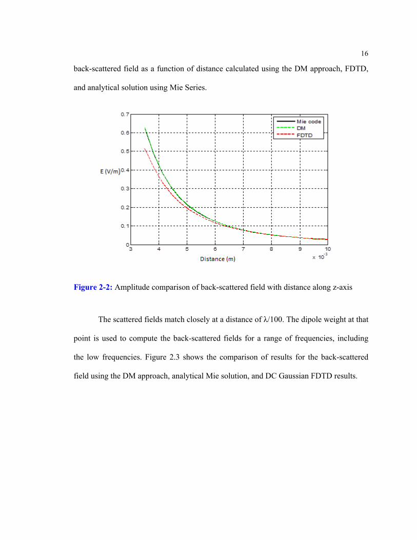
field, the corresponding dipole moment weights Il are obtained. Figure 2.2 compares the
Figure 2-1: PEC sphere illuminated with X-polarized, Z-directed incident electric field
16
back-scattered field as a function of distance calculated using the DM approach, FDTD,
and analytical solution using Mie Series.
Figure 2-2: Amplitude comparison of back-scattered field with distance along z-axis
The scattered fields match closely at a distance of λ/100. The dipole weight at that
point is used to compute the back-scattered fields for a range of frequencies, including
the low frequencies. Figure 2.3 shows the comparison of results for the back-scattered
field using the DM approach, analytical Mie solution, and DC Gaussian FDTD results.

17
Figure 2-3: Amplitude variation with frequency comparison at a point λ/100
2. PEC Cylinder
Using the same approach, the PEC sphere was replaced by a cylinder with a
radius of λ/200 and height of λ/100 as shown. The following results in Figure 2.5 and
Figure 2.6 were obtained.
Figure 2-4: PEC cylinder

18
Figure 2-5: Amplitude variation with distance along z-axis for PEC cylinder
Figure 2-6: Variation of Ex with frequency at observation point for PEC cylinder

19
3. PEC Cube
The procedure was similarly done for a cube with a length of λ/100 at 500Mhz.
The results obtained for the cube are shown
Figure 2-7: PEC cube
Figure 2-8: Variation of Ex with distance z-axis for a cube

20
Figure 2-9: Variation of Ex with frequency at observation point 9 mm along z-axis for a cube
2.4.2 Observations
For the case of the sphere, the DM approach results closely match the analytical
results from the Mie Series. The DM method was able to obtain accurate lower-frequency
results when compared to those from the FDTD simulations. The back-scattered electric-
field results from the geometric shapes show three regions of variations of the Ex with
frequency: the lower frequency region where the DM approach has results that closely
match with the analytical results for a sphere; the overlapping region where the results
from the DM approach and FDTD are the same; and the higher frequency region, where
FDTD results are more accurate.

21
2.5 Dipole Moment Technique: Far-Field Patterns Method
The steps for the computation of the low-frequency dipole moment are as follows:
1. For a given arbitrary shape of an object, a single frequency (sine) wave is used as
the incident electric field Ei on the object.
2. The scattered electric far-field pattern is obtained.
3. The scattered far-field electric pattern is used to extract the weights of the electric
dipole moments Ilx, Ily, Ilz.
4. Using the obtained electric dipole moments, the electric field due to the dipole
moments can be obtained. It is well established that the analytical solution for
dipole moments is the same as the Mie series solution for a PEC sphere.
5. Given the extracted weights of the dipole moments at the given single frequency,
the weights can be used to obtain the scattered electric field at that frequency and
other frequencies, including very low frequencies, and also at any distance away
from the scatterer.
2.5.1 Mathematical Proof of Method
Given E!"(r,θ ,φ) = a1
"ϕx + a2
"ϕy + a3
"ϕz , where E
!" is the combined far field pattern
from the electric dipoles, !ϕx , !ϕy and
!ϕz are dipole patterns obtained from the orientation
of x, y, and z respectively. For the method to work, we have to show:
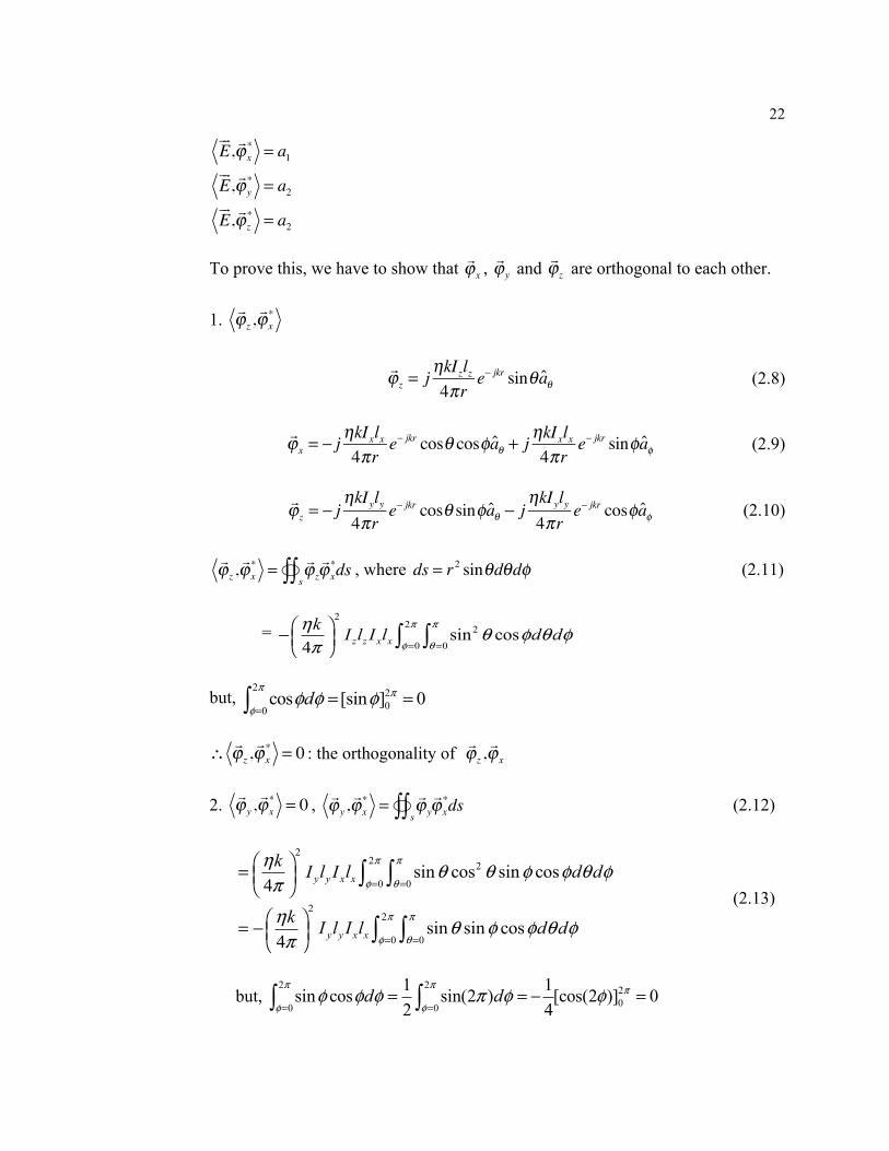
22
E!", "ϕx
* = a1
E!", "ϕy
* = a2
E!", "ϕz
* = a2
To prove this, we have to show that !ϕx , !ϕy and
!ϕz are orthogonal to each other.
1. !ϕz ,!ϕx*
!ϕz = jηkIzlz
4πre− jkr sinθ aθ (2.8)
!ϕx = − jηkIxlx
4πre− jkr cosθ cosφaθ + j
ηkIxlx4πr
e− jkr sinφaφ (2.9)
!ϕz = − j
ηkIyly4πr
e− jkr cosθ sinφaθ − jηkIyly4πr
e− jkr cosφaφ (2.10)
!ϕz ,!ϕx* =
!ϕzs"∫∫!ϕx*ds , where ds = r2 sinθdθdφ (2.11)
=
but,
∴!ϕz ,!ϕx* = 0 : the orthogonality of
!ϕz ,!ϕx
2. !ϕy ,!ϕx* = 0 ,
!ϕy ,!ϕx* =
!ϕys"∫∫!ϕx*ds (2.12)
(2.13)
but,
22 2
0 0sin cos
4 z z x xk I l I l d d
π π
φ θ
η θ φ θ φπ = =
⎛ ⎞−⎜ ⎟⎝ ⎠ ∫ ∫
2 200
cos [sin ] 0dπ π
φφ φ φ
== =∫
22 2
0 0
22
0 0
sin cos sin cos4
sin sin cos4
y y x x
y y x x
k I l I l d d
k I l I l d d
π π
φ θ
π π
φ θ
η θ θ φ φ θ φπ
η θ φ φ θ φπ
= =
= =
⎛ ⎞= ⎜ ⎟⎝ ⎠
⎛ ⎞= −⎜ ⎟⎝ ⎠
∫ ∫
∫ ∫
2 2 200 0
1 1sin cos sin(2 ) [cos(2 )] 02 4
d dπ π π
φ φφ φ φ π φ φ
= == = − =∫ ∫

23
∴!ϕy ,!ϕx* = 0
shows the orthogonality of
!ϕy ,!ϕx .
3. !ϕz ,!ϕy* = 0 ,
!ϕz ,!ϕy* =
!ϕz!ϕy*
s"∫∫ ds (2.14)
= − ηk4π
⎛⎝⎜
⎞⎠⎟2
Izlz Iyly sin2θ=0
π
∫φ=0
2π
∫ θ cosθ sinφdθdφ (2.15)
but ,
∴!ϕz ,!ϕy* = 0 , shows the orthogonality of
!ϕz ,!ϕy
By duality principles, we can use the same procedure to show the orthogonality of
magnetic dipole moments and use them to represent magnetic materials.
2.5.2 Electric Fields Radiated by X-, Y-, Z- Oriented Dipole Moments
The z-component of the fields produced at observation point (xi, yi, zi) by a z-
directed dipole moment centred at (xs, ys, zs) can be expressed as:
Ezz = Er cosθ − Eθ sinθ (2.16)
Given the following electric field equations for the dipole moments,
Er =Il2π
e− jkr ηr2
+ 1jωεr3
⎛⎝⎜
⎞⎠⎟cosθ = er cosθ (2.17)
Eθ =Il4π
e− jkr jωµr
+ ηr2
+ 1jωεr3
⎛⎝⎜
⎞⎠⎟sinθ = eθ sinθ (2.18)
by explicating the dependence upon x, y, z, we can write the electric field due to the z-
directed dipole:
2 200
sin [cos ] 0dπ π
φφ φ φ
== − =∫

24
Ezz = er cos2θ − eθ sin
2θ = er(zi − zs )
2
r2− eθ
(xi − xs )+ (yi − ys )r2
(2.19)
Applying the same calculation for the other components of the z-directed dipole and
rotating the coordinate system for the x- and y- directed dipoles, the fields are obtained
for z-directed dipole moments:
Exz = (er + eθ )(xi − xs )(zi − zs )
r2
Eyz = (er + eθ )(yi − ys )(zi − zs )
r2
Ezz = er(zi − zs )
2
r2− eθ
(xi − xs )2 + (yi − ys )
2
r2
(2.20)
for x-directed dipole moments:
Exx = er(xi − xs )
2
r2− eθ
(yi − ys )2 + (zi + zs )
2
r2
Eyx = (er + eθ )(xi − xs )(yi − ys )
r2
Ezx = (er + eθ )(xi − xs )(zi − zs )
r2
(2.21)
and for y-directed dipole moments:
Exy = (er + eθ )(xi − xs )(yi − ys )
r2
Eyy = er(yi − ys )
2
r2− eθ
(xi − xs )2 + (zi − zs )r2
Ezy = (er + eθ )(yi − ys )(zi − zs )
r2
(2.22)
Given the weights of dipole moments from the far-field patterns, one can compute
the scattered far fields at lower frequencies and at any other distance around the scatterer
using the equations.

25
2.5.3 Numerical Results
1. PEC Sphere
For the first example, we again consider a PEC sphere with diameter λ/100. It is
illuminated by a single-frequency (500 MHz) plane wave, incident along z-axis with Ex
polarization, as shown in Figure 2.10.The far-field pattern approach was used to compute
the dipole moments.
Figure 2-10: PEC sphere illuminated with X-polarized, Z-directed incident electric field
The x-directed dipole moment was used for this case. The back-scattered field
was computed from λ/100 on the z-axis using the dipole moment. Figure 2.11 compares
the back-scattered field as a function of distance calculated using the DM approach,
FDTD, and the analytical solution using Mie Series.

26
Figure 2-11: Amplitude comparison of back-scattered field with distance along z-axis
The x-directed dipole weight is used to compute the back-scattered fields for a
range of frequencies including the low frequencies. Figure 2.12 shows the comparison of
results for back-scattered fields using the DM approach, analytical Mie solution, and DC
Gaussian FDTD results.

27
Figure 2-12: Variation of Ex with frequency at observation point for PEC sphere
2. PEC Cone
Using the same far field approach, the PEC sphere was replaced by a cone with a
radius of λ/200 and height of λ/200 as shown in Figure 2.13. The following result in
Figure 2.14 was obtained.
Figure 2-13: PEC cone

28
The procedure was similarly done for a cone cylinder with a length of λ/100 and
height of λ/200. The results obtained are shown below
Fig 2-15: PEC cone cylinder
Figure 2-14: Variation of Ex with frequency at observation point for PEC cone

29
Figure 2-16: Variation of Ex with frequency at observation point 9 mm along z-axis for the cylinder
2.6 Conclusions
In this chapter we have used two different Dipole Moment Approaches to solve
scattering problems for single scatterer. For the case of the sphere, the DM approach
results were shown to closely match the analytical results from the Mie Series. The DM
method was able to obtain lower frequency results that were accurate when compared to
those from the FDTD simulations. The back-scattered electric field results from the
geometric shapes show three regions of variations of the Ex with frequency: the lower
frequency region where the DM approach has results that match closely with the
analytical results for the sphere; the overlapping region where the results from the DM
approach and FDTD are the same; and the higher-frequency region where FDTD results
are most accurate.

30
Chapter 3
Multiple Scattering using the Dipole Moment Approach
3.1 Introduction
In the case of more than one scatterer, or where we have a complex object, the
procedures developed in the previous chapter would not give a satisfactory solution to the
problem because more dipole moments will be required to represent the problem. In this
chapter we present techniques for dealing with multiple scatterers that apply to a group of
particles that can model proppants in hydraulic fractures.
3.2 Dipole-Moment Formulation for Multiple-Scattering Objects
The analytical dipole moment solutions for the scattered field created by a sphere
were developed and presented in the previous chapter. The derived field expressions are
valid for both dielectrics and PEC spheres. By applying an equivalent theory, the field
expressions for a magnetic sphere can be obtained. From the previous work, we have
learned that a small sphere can be replaced by its equivalent dipole moments while
working at “large” distances from the small sphere. However, it has been mathematically
verified that these dipole-moment approximations are valid in all regions, irrespective of
distance as long as the point of observation is located outside a sphere circumscribing the
object, assumed to be small compared to the wavelength [33]. The electric dipole

31
moment goes to zero for magnetic materials, and similarly the magnetic dipole moment
goes to zero for non-magnetic materials. For a complete representation of an arbitrary
scatterer with magnetic and dielectric properties, we need a total of 3 electric dipole and 3
magnetic dipole moments [31].
3.2.1 Modeling Using Spheres
Based on the Dipole Moment theory already developed, there exists a way to
model objects and fine structures whose sizes are much smaller than the wavelength of
the incident field. The objects are first replaced with a bunch of spheres, which we can
then replace with unknown dipole moments. The method of moments can then be
effectively deployed to solve for unknown dipole moments [34]. Once the unknown
dipole moments are obtained, the information can be used to compute the fields
everywhere around the objects [35].
3.2.2 Consistency Factor Computation
It is important to remember that the dipole moment specified and derived
previously is equivalent to a single-point representation of the scatterer. However, when
we are dealing with dielectrics and magnetic spheres—which are quite unlike PEC
spheres—fields exist inside the above spheres; hence we must find an equivalent volume
representation of the dipole moments of those fields. One simple way of getting the
equivalent volume representation is to assume that the final distributed dipole moment is

32
a constant value (F), multiplied by the condensed value. The constant number is denoted
by F and is called the Consistency Factor, which can be found for a single sphere using
the steps below:
A single sphere of diameter 2a is considered with the origin at its center.
Let the consistency factor be F.
Il represents the condensed dipole moment of a single sphere.
We match the polarization currents at the center of the sphere to give:
𝜖𝜖 𝜖𝜖 − 1 𝑬𝑬 + 𝑬𝑬 = 𝐹𝐹. 𝐼𝐼𝐼𝐼 (3.1)
where 𝐸𝐸 = 𝐸𝐸 - the incident electric field at the center of the sphere
𝐼𝐼𝐼𝐼 = 𝐸𝐸 𝑘𝑘𝑘𝑘 (3.2)
is the single-point dipole moment
𝑬𝑬 = − 𝑒𝑒 + + 𝑠𝑠𝑠𝑠𝑠𝑠 ≈ − (3.3)
is the scattered field (assuming 𝑘𝑘𝑘𝑘 → 0: 𝑠𝑠𝑠𝑠𝑠𝑠𝑠𝑠𝑠𝑠: 𝑠𝑠𝑠𝑠𝑠𝑠𝑠𝑠𝑠𝑠 𝑠𝑠𝑠𝑠ℎ𝑒𝑒𝑒𝑒𝑒𝑒 ).
By solving the above equation, we obtain:
𝐹𝐹 ≈−3𝑗𝑗4𝜋𝜋𝜋𝜋𝑎𝑎
In the above solution, the polarization currents were matched instead of applying
boundary conditions. This is because the quantities we are dealing with are distributed in
volume; hence it is better to match the polarization currents instead. This condition is
termed the Consistency Condition. It should be noted that the scattered fields were

33
calculated on the surface of the sphere, and it is assumed that the fields will be the same
at the center. This holds because the sphere is very small compared to the wavelength and
has no room for field variations inside it. It also bypasses the singularity, which occurs
when we try to calculate the field at the center and which is a major problem in the
conventional method of moments (MOM) technique.
3.3 Dipole Moment–MOM Formulation
In formulating the Method of Moment problem, we assume the consistency factor
F to be the same, irrespective of whether the sphere is independent or in a group.
To show the method, we consider a rod oriented along 𝑦𝑦, extending from − to
+ and of thickness d. We replace the rod with a string of N spheres of diameter d=2a,
making sure that l =Nd.
Since the incident field can be arbitrary, depending on the problem at hand, the
spheres are going to be replaced with three equivalent independent dipole moments—one
in each direction. The formulation then goes as follows:
Let 𝐼𝐼𝐼𝐼 represent the effective dipole moment of the 𝑛𝑛 sphere directed along 𝑠𝑠.
Let 𝐸𝐸 be the incident field component at the center of the nth sphere along 𝑠𝑠
We form the matrix by applying the consistency condition at the center of each
sphere for each component.
Applying the consistency condition for the 𝑥𝑥-directed dipole moment of n =1, i.e.,
for the 1st sphere, we obtain:

34
𝜖𝜖 𝜖𝜖 − 1 𝐸𝐸 + 𝐸𝐸 + 𝐸𝐸 + 𝐸𝐸 + 𝐸𝐸 + 𝐸𝐸 +. .+𝐸𝐸 + 𝐸𝐸 +
𝐸𝐸 +. .+𝐸𝐸 = 𝐹𝐹𝐹𝐹𝑙𝑙 (3.4)
We repeat this procedure for other spheres up to n=N, i.e. Nth sphere, and for it
we obtain:
𝜖𝜖 𝜖𝜖 − 1 𝐸𝐸 + 𝐸𝐸 + 𝐸𝐸 +. .+𝐸𝐸 + 𝐸𝐸 + 𝐸𝐸 +. .+𝐸𝐸 + 𝐸𝐸 +
𝐸𝐸 +. .+𝐸𝐸 = 𝐹𝐹𝐹𝐹𝑙𝑙 (3.5)
For the 𝑦𝑦-directed dipole moment of n=1, i.e., for the 1st sphere, we obtain:
𝜖𝜖 𝜖𝜖 − 1 𝐸𝐸 + 𝐸𝐸 + 𝐸𝐸 +. .+𝐸𝐸 + 𝐸𝐸 + 𝐸𝐸 +. .+𝐸𝐸 + 𝐸𝐸 +
𝐸𝐸 +. .+𝐸𝐸 = 𝐹𝐹𝐹𝐹𝑙𝑙 (3.6)
We repeat this procedure for other spheres up to n=N, i.e. for the Nth sphere, and
for it we obtain:
𝜖𝜖 𝜖𝜖 − 1 𝐸𝐸 + 𝐸𝐸 + 𝐸𝐸 +. .+𝐸𝐸 + 𝐸𝐸 + 𝐸𝐸 +. .+𝐸𝐸 + 𝐸𝐸 +
𝐸𝐸 +. .+𝐸𝐸 = 𝐹𝐹𝐹𝐹𝑙𝑙 (3.7)
For the 𝑧𝑧-directed dipole moment of n=1 i.e. for the 1st sphere, we obtain:
𝜖𝜖 𝜖𝜖 − 1 𝐸𝐸 + 𝐸𝐸 + 𝐸𝐸 +. .+𝐸𝐸 + 𝐸𝐸 + 𝐸𝐸 +. .+𝐸𝐸 + 𝐸𝐸 +
𝐸𝐸 +. .+𝐸𝐸 = 𝐹𝐹𝐹𝐹𝑙𝑙 (3.8)
We repeat this procedure for other spheres up to n=N i.e. Nth sphere, and we
obtain:
𝜖𝜖 𝜖𝜖 − 1 𝐸𝐸 + 𝐸𝐸 + 𝐸𝐸 +. .+𝐸𝐸 + 𝐸𝐸 + 𝐸𝐸 +. .+𝐸𝐸 + 𝐸𝐸 +
𝐸𝐸 +. .+𝐸𝐸 =𝐹𝐹𝐹𝐹𝑙𝑙 (3.9)

35
The self-terms in all the equations, namely 𝐸𝐸 , are computed on the surface of
the sphere instead of at the center—in turn getting rid of singularity.
From the above equations, we have obtained 3N variables and 3N equations that
would enable us solve for Il’s or for the E’s, which gives Il’s when multiplied by
𝑘𝑘𝑘𝑘 . After solving the equations, we can use Il’s to calculate the field
produced. Hence we have the solution to the problem.
We can follow the same procedure for magnetic materials using the equivalent
theorem. We now give examples of application of this technique used to solve scattering
problems involving multiple particles.
3.3.1 Examples of Magneto Dielectric Random Spherical Particles Scattering Problems
We consider a random distribution of 14 spherical particles with a mean diameter
of 1mm and a standard deviation of 0.3 mm. Here, because the particles are small in
number, we are able to know the exact location of each particle and its dimensions. Then
we can apply the Dipole Moment Formulation for multiple scattering to obtain the
scattered field. The complex permittivity and permeability of the material for the sphere
are given as 36+0.2i and 16+2i respectively. An x-directed, Ez polarized incident wave
was used to excite the particles at a frequency of 500 MHz, which is not a very low
frequency, to enable us to compare with an FDTD method. The arrangement of the
scattering problem is shown below.
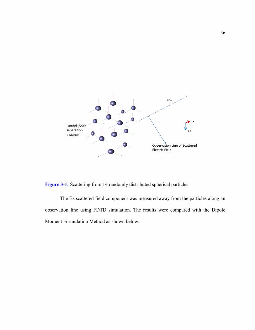
36
Figure 3-1: Scattering from 14 randomly distributed spherical particles
The Ez scattered field component was measured away from the particles along an
observation line using FDTD simulation. The results were compared with the Dipole
Moment Formulation Method as shown below.

37
Figure 3-2: Validation of DM with FDTD: scattered electric Field (Ez) on a line
The simulation for the FDTD was done at a mid frequency of 500 MHz to enable
us compare the results with the Dipole Moment formulation, and the two results were
found to be in agreement.
This example was done with only a few particles. However, in real life, there are a
lot of particles and we cannot know their exact position at any given time because they
are in constant random motion. In this case, we must employ statistical techniques to
characterize the particle materials.

38
3.4 Monte Carlo Techniques
We present description of the Monte Carlo simulations of multiple particles in
random placement as it may occur when proppants are pumped to create a fracture. The
placement of the particles is assumed to be discrete, and the medium is dense. There are
two commonly used Monte Carlo techniques in generating particle positions for
simulation, namely, the Metropolis Algorithm and Sequential Addition techniques [36].
For both techniques, it is assumed the particles are in a cubic box to generate their
positions randomly, the forces of interaction among particles is negligible, and there is no
penetration when the particles collide. In the Metropolis algorithm, the particles are
initially assigned positions and then are reshuffled using random walk to create new
realizations of particle positions. In contrast, the Sequential Addition Method works not
by reshuffling particles, but by adding particles in serial and random manner into the box
to create different realizations. To position the particles and represent the simulation
accurately, several realizations are used.
The definition of the joint probability density distribution function of the proppant
particles is used in calculating the particle-pair distribution functions. This is done by
enumerating the number of times a separation of the proppant particles pair occurred as
related to the separation distance and averaging them over the realizations. We imposed
boundary conditions of periodic type at the walls of the cubic box to take into account the
edge effects of the box.
We performed computer simulation experiments on a model with spherical
proppants N. The N particles with varying diameter are put in a cube box of width l. We

39
assume Ni to be the number of particles with radius ai in the box. We can find the
number density ni and the fraction of volume fi of the particles with radius ai as follows
[37]:
𝑛𝑛 = (3.10)
𝑓𝑓𝑓𝑓 = 𝑛𝑛𝑛𝑛 𝑎𝑎 (3.11)
𝑁𝑁 = 𝑁𝑁 (3.12)
𝑓𝑓 = 𝑓𝑓 (3.13)
where f represents the fraction of the total volume particles occupy in the box.
The pair-distribution function of the particles approaches 1 as the distance
between them increases, which mean the positions of particles are independent when the
particles are further apart. The N particles, when placed inside the cubic box with the
periodic boundary conditions, create images with each image cube containing N particles
having the same geometric arrangement of particle positions as that in the main cubic
box.
The spherical proppant particles initially are randomly positioned in the primary
cubic box with no overlap among them. Shuffling particles as follows generates new
realizations of the position of the particles. In each cycle of movement, each particle is
subject to random displacement once. The new position of the particle following
displacement is accepted based on whether the position of the particle coincides with
another or not. The displacement is simulated as a random motion that is not affected by

40
forces of attraction among particles and in which a particle does not penetrate other
particles during collision. It should be noted the particles do not move physically and that
the introduction of particles displacement during the process is to create new
configurations and realizations of possible movement of the particles. We follow the
procedure in [38] to implement the algorithm using the following steps:
1: Configure the system initially.
The proppant particles are assigned three-dimensional coordinates within the
cubic box to initially configure the system. We assume a 1 cubic meter box so that the
rectangular coordinates of particles are in the range [0,1}. We can obtain the initial
configuration of all the particles by placing them in a periodic spatial distribution in the
cube or just assigning them random positions.
2: Reconfigure the system by random displacement of proppants.
The simulation continues with displacing the particles sequentially. The following
relationship determines the new trial position of a particle during the displacement
motion:
𝑥𝑥⟶ 𝑥𝑥 + ∆ 𝑦𝑦⟶ 𝑦𝑦 + Δ 𝑧𝑧⟶ 𝑧𝑧 + Δ where x, y, and z are the
coordinates of the proppant particles and ∆ is the maximum displacement permitted for
each change of position. The 𝜂𝜂 𝑖𝑖, i = 1,2,3, are generated as random numbers, with
uniform distribution independently in [-l, l]. A particle can be at any position in a small
cube of 2𝑙𝑙Δ from its initial position after the displacement takes place. The displacement
criteria of a particle have to meet the periodic boundary conditions of the particle
reentering the cube from the opposite side when the particle is displaced beyond the
length of the cube on one side during the simulation. If during simulation, the position of

41
a spherical particle move to new coordinate 𝑥𝑥 𝑦𝑦 𝑧𝑧 in current stage, and when x' > l, or
x' < 0, its new location will be x' - l, or x' + l. Similar procedure is used for the y- and z-
coordinates. If the displacement value A is too small, displacement would be accepted,
but if it were too large, the algorithm would reject the displacement. Setting the
acceptance rate Ac between 30% and 70% is the rule of thumb for the simulation.
3: Confirm acceptance of displacements.
If the new position of the particle after displacement does not overlap with that of
another particle, the new displacement position is accepted and the location of the
proppant particle displaced are updated. On the other hand, the displacement is rejected
and the proppant is returned to its initial location. The percentage of new positions
accepted is determined by the value of the maximum displacement set. Checking
overlapping of proppants is straightforward, but we must be careful in cases of position
of two proppants that do not coincides in the center of cube but their images in the next
cube are in the forbidden domain of each other.
4: Update Configuration numbers generated.
Keep count of the number of configurations by adding 1 to the counter. This
should be done even when particle displacement at a given stage of Step 2 is not
accepted, because this non-acceptance is taken as a new position configuration of the
proppants. A new particle configuration implies each of the particles has been subject to
one displacement attempt even if the displacement is not accepted. Every counted
configuration is referred to as a realization. Therefore, between two realizations, each of
the particles has been displaced an average number of NcAc, where Ac is the rate of
acceptance in the simulation.

42
5: Enumerate the number of times pair separation differences occurred.
The above steps are repeated several times to generate several realizations and to
count the number of pair of separation differences occurring during the simulation.
Example 3.2: We consider a case of a box with a random distribution of 4000
particles as shown in the figure below. We find the positions of particles using the
Metropolis Algorithm as described above.
Figure 3-3: Discrete random distribution of particles in a 1-meter cube box
After obtaining the positions of particles, we use the information to set up a
Dipole Moment solution to obtain scattered fields from their random distribution. The
sizes of the particles are generated from a Gaussian distribution of Mean = 1 mm,
0.20.4
0.60.8
0.20.4
0.60.8
0.2
0.4
0.6
0.8
centers x coordinate
Problem Discretization
centers y coordinate

43
Standard Deviation = 0.3 mm. The particles have Dielectric Constant = 36+0.2i and
Relative Permeability 16+ 0.1i. The Incident Electric Field Frequency used is 500MHz.
Figure 3-4: Incident field set up for the simulation on 1 meter cube box
We have run the simulation for 4000 particles to obtain different 300 realizations.
The graph below shows the plot of scattered Electric Fields. The plot shows the average
of the scattered fields and samples of scattered fields from the 1 and 9 realizations.

44
Figure 3-5: Graph showing the mean of the ensemble realizations and individual realizations
We have computed the variance and standard deviation of the realizations and
have plotted them in Figure 3.6 and Figure 3.7, which shows that the variance and
standard divisions among the realization are small are for dense particle distribution.
Figure 3-6: Variance of ensemble realizations
0 0.1 0.2 0.3 0.4 0.5 0.6 0.7 0.8 0.9 11.2
1.4
1.6
1.8
2
2.2
2.4
2.6
2.8x 10⁻⁵
distance (m)
V/m
Ex
Exsaverage
Exs9Exs1

45
Figure 3-7: Standard Deviation of the realizations
The results show that we would not need to run simulations with several
realizations and that we can obtain good results using a single realization for the case of
densely distributed particles.
We then varied the size of the enclosure containing the particles while keeping the
particle density constant to see the effect of the size of the box upon the particles. The
figure below shows the relationship in the case of a cube.

46
Figure 3-8: Plot shows a linear relationship between the volume of particles in different cube sizes and scattered electric fields.
Example 3.3: We repeat the same procedure as in example 1 for the case of a
cuboid, as shown below, with a different depth and with fixed cross sections.
0 0.1 0.2 0.3 0.4 0.5 0.6 0.7 0.8 0.9 10
0.5
1
1.5
2
2.5
3x 10⁻⁵ Volume vs Scattered Field
Volume (m3)
Ex
Fiel
d

47
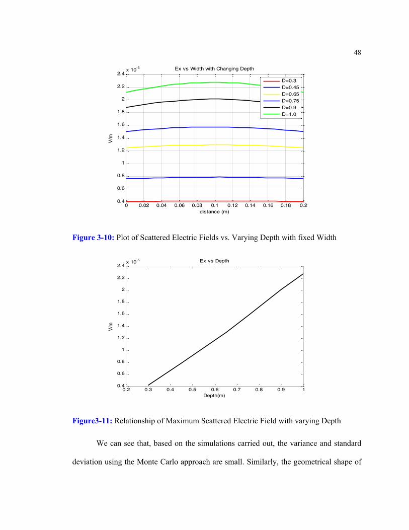
Figure 3-9: The depths of the cuboid were D(m)=[0.3, 0.45, 0.65, .75, 0.9, 1]
For each depth, we measured the scattered field across the cross-section, which is
plotted as shown below.
48
Figure 3-10: Plot of Scattered Electric Fields vs. Varying Depth with fixed Width
Figure3-11: Relationship of Maximum Scattered Electric Field with varying Depth
We can see that, based on the simulations carried out, the variance and standard
deviation using the Monte Carlo approach are small. Similarly, the geometrical shape of
0 0.02 0.04 0.06 0.08 0.1 0.12 0.14 0.16 0.18 0.20.4
0.6
0.8
1
1.2
1.4
1.6
1.8
2
2.2
2.4x 10⁻⁵
distance (m)
V/m
Ex vs Width with Changing Depth
D=0.3D=0.45D=0.65D=0.75D=0.9D=1.0
0.2 0.3 0.4 0.5 0.6 0.7 0.8 0.9 10.4
0.6
0.8
1
1.2
1.4
1.6
1.8
2
2.2
2.4x 10⁻⁵ Ex vs Depth
V/m
Depth(m)

49
the cube and cuboid shows a linear relationship of the volume of particles and the
scattered field. We can then think of comparing this result to mixing-rules-equivalent
medium theory to see what significant differences there are, and to make decision about
which approach to use.
3.5 Conclusion
In this chapter the dipole moment approach for multiple scatterers was formulated
and examples were provided to validate it with FDTD at medium frequencies. We have
introduced a Monte Carlo type of statistical technique, in particular the Metropolis
Algorithm, to simulate positions of random particles with different diameters and applied
to study scattering properties of magneto dielectric materials that can be used in making
proppants. Several examples are given for particles of different shapes and their scattered
fields were computed by using the approach.

50
Chapter 4
Mixing Rules and Materials Properties for Proppants
4.1 Introduction
The Dipole Moment (DM) approach is useful for studying the scattering
characteristics of small amounts of samples of materials; however, when the sample size
becomes large, the associated matrix of the solution grows exponentially, making it
difficult to solve numerically without the help of additional methods such as the
Characteristic Basis Function Method (CBFM) [39]. However, even with CBFM, the
approach becomes untenable when dealing with a problem involving multiphase
mixtures. To circumvent this problem, in this chapter we introduce some mixing rules for
magnetic materials for use as smart proppants. There are several types of mixing
formulas in the literature, and the challenge is to decide which one to apply in a given
situation to obtain accurate results from the analysis. We compare the results of the
Dipole Moment approach with those from three common mixing formulas, to choose a
mixing formula that yields results close to the ones from Dipole Moment approach.
Before we get into that, we give an overview of a standard constitutive parameters
retrieval method, which uses the transmission/reflection method to obtain the permittivity
and permeability parameters of a material when dealing with new materials for which the
values are not available in the research literature.

51
4.2 Properties of Proppants and Their Slurry
The operational environment in oil and gas reservoir shale is harsh, with extremely
high temperatures, pressures and depths. Temperatures can reach as high as 400K,
pressure of 20,000 bars and depth of 6000 feet. Because of these conditions, the
proppants and slurry to use for magnetic sensing must meet certain requirements, such as:
1. It can be pumped in to the borehole under high pressures.
2. It can be forced into the cracks, fissures, and voids produced by hydrofracturing
of a localized region of shale reservoir in the horizontal region of the well.
3. It must be capable of carrying a good volume of ferromagnetic proppants.
4. The mixture must not dissolve the particles by chemical reaction or due to the
high temperature in the well.
5. The size of the particles must be sufficient to exhibit true ferromagnetic behavior.
The list of materials that can be produced in the form of small particles and satisfy the
requirement of high Curie-Weiss temperature, Tc, is essentially limited to iron and a few
iron compounds such as Magnetite, Hematite, etc.
Important factors in the slurry are the relationships between proppant particle size and
shape and the direction of the spontaneous magnetization of the mixture. The effect of the
shape is that if the particles are spherical, the internal magnetization would not have any
tendency to align with respect to a set of axes fixed to the particle. In the case of particles
that have elongated shapes, the internal magnetization may tend to align parallel to the

52
long axis of the particle. If the viscosity of the slurry is low enough to permit rotation, it
is also possible that the Earth’s magnetic field can exert weak forces to align the particles.
The magnetic permeability of a material is based upon the intrinsic property of the
particles and their distribution. The magnetic permeability of material can be expressed
as a function of size, size-distribution, temperature, concentration, and the intrinsic
material properties related by the Langevin Equation [40]. The equation gives the
magnetic susceptibility χ as:
(4.1)
φ is the volume fraction of particles
µ0 is the permeability of free space (4π*10-7 Wb/A.m)
Md is the saturation magnetization of the material at the absolute temperature T
d is the particle diameter (assume spherical particles)
k is the Boltzmann Constant
The magnetic susceptibility is related linearly to magnetic permeability:
(4.2)
The plot below shows the relationship of the magnetic susceptibility of magnetite
with saturation magnetization Md of bulk magnetite, particles with varying diameter and
different volume of inclusions.
χ = π18
φµ0Md
2d 3
kT
µ = 1+ χ

53
Figure 4-1 Susceptibility of Material vs. Volume in a Mixture
4.3 Retrieval of Permeability and Permittivity Of Materials Using Transmission/Reflection Methods
There are several techniques for obtaining permittivity and permeability of materials
depending on the frequencies of interest [41]. At frequencies below 10 MHz, the
transmission/reflection methods provide good estimates of these parameters [42,43]. In a
situation where a new technique is used to create a material, these parameters are not
known, and an experimental approach is used to find them.
In the transmission/reflection method, S-parameters are calculated by using a wave,
which is normally incident on a slab of material. The effective refractive index n and
-parameters [22]. The permittivity ε and
permeability µ are then directly calculated from ε=nZ and µ=n/Z. We define the transfer
matrix T for a one-dimensional slab [44]:

54
(4.3)
where
F =
!E!Hred
⎛
⎝⎜⎞
⎠⎟ (4.4)
E and Hred are the complex electric and magnetic amplitudes. The magnetic field
is the reduced form with normalization !Hred = (+ jωµ0 )
!H . The transfer matrix for a
homogeneous 1D slab has the form:
(4.5)
The amplitudes and phases of the scattered field can be measured with a network
analyzer to yield the scattering matrix [S] that relates the amplitudes of the incident,
transmitted and reflected fields and experimentally determined quantities.
The T-matrix and S- matrix elements are related by the equations [45]:
S11 =T11 −T22 + jkT12 −
T21jk
⎛⎝⎜
⎞⎠⎟
T11 +T22 + jkT12 +T21jk
⎛⎝⎜
⎞⎠⎟
(4.6)
S12 =2det(T )
T11 +T22 + jkT12 +T21jk
⎛⎝⎜
⎞⎠⎟
(4.7)
S21 =2
T11 +T22 + jkT12 +T21jk
⎛⎝⎜
⎞⎠⎟
(4.8)
F ' = TF
T =T11 T12T21 T22
⎛
⎝⎜
⎞
⎠⎟ =
cos(nkd) − Zksin(nkd)
kZsin(nkd) cos(nkd)
⎛
⎝
⎜⎜⎜⎜
⎞
⎠
⎟⎟⎟⎟

55
S22 =T22 −T11 + jkT12 −
T21jk
⎛⎝⎜
⎞⎠⎟
T11 +T22 + jkT12 +T21jk
⎛⎝⎜
⎞⎠⎟
(4.9)
From Eqn. (4.5), it can be seen that the S matrix is symmetric for a homogeneous
slab, ie.,T11=T22=Ts, and det(T)=1. Thus,
S11 = S22 =
12
T21jk
− jkT12⎛⎝⎜
⎞⎠⎟
Ts +12
jkT12 +T21jk
⎛⎝⎜
⎞⎠⎟
(4.10)
Substituting for the analytical expressions of the T-matrix elements in Eqn. (4.5)
results in:
S11 = S22 =j21z− z⎛
⎝⎜⎞⎠⎟ sin(nkd) (4.11)
and
S21 = S12 =1
cos(nkd)− j2
z + 1z
⎛⎝⎜
⎞⎠⎟ sin(nkd)
(4.12)
Inverting equation (4.11) and (4.12), we can obtain n and Z in terms of the
scattering parameters S11 and S21:
(4.13)
(4.14)
Eqns. (4.13) and (4.14) provides a complete description of the material properties of
the homogeneous slab from which the permittivity ε and permeability µ are calculated
n = 1kdcos−1 1
2S21(1− S11
2 + S212⎡
⎣⎢
⎤
⎦⎥
Z = (1+ S11)2 − S21
2
(1− S11)2 − S21
2

56
[45]. The exact determination of material parameters is possible, without ambiguities, if
the wavelength within the medium is much larger than the slab length, which is the case
in sensing proppants in fractures.
4.4 Effective Medium Theory
Effective medium theory is used to describe macroscopic properties of dielectric
and magnetic mixture materials in a medium. The effective permittivity can be derived
from a solution to the electrostatic problem used to describe the properties of dielectric
mixtures [46]. The effective magnetic permeability corresponds to the ratio between the
applied magnetic field and average magnetic displacement, which is the average
magnetic polarization in a heterogeneous medium. The Laplace equation for the potential
and its boundary conditions is similar for both electrostatic and magnetostatic problems.
The numerous dielectric-mixing formulas can therefore be written for the equivalent
effective permeability of magnetic mixtures using the duality principles [47].
The wavelength of the applied field is assumed to be larger than the characteristic
distance of the inhomogeneity of the heterogeneous medium, which implies that the
effective medium theory for permeability and permittivity is a low-frequency concept
that is applicable to the fracture problem we are dealing with. The averaging of
polarization is carried out in a scale smaller than the spatial variation of the wavelength
incident electromagnetic field to satisfy the quasistatic-form Maxwell equations. It has
been shown [48] that the limit for the dimension of the scatterer is where dmax
is the maximum dimension of the inclusion, and λ is the wavelength of the incident field.
dmax !
λ2π

57
The interactions due to the permittivity and permeability of a material are normally
different for the dielectric and magnetic materials. Nonlinearity and temperature above
Curie temperature significantly affect the behavior of magnetic mixtures when compared
to dielectric mixtures.
4.4.1 Mixtures with Spherical Inclusions
We consider a two-phase heterogeneous mixture consisting of a background medium
with permeability, µ0, and spherical proppants with inclusions of permeability µ1. In low-
frequency limits, where dimensions of the proppants are smaller than the wavelength, the
scattering effects of the inclusions are negligible. The magnetic flux density is given by:
B!"= µeff H
!"! (4.15)
where µeff is the effective magnetic permeability. Expressing B in terms of
average magnetic polarization Jm, we can write:
B!"= µoH!"!
+ J!"
m (4.16)
The average magnetic polarization is Jm given by:
J!"m = n j
" (4.17)
where n is the number of inclusions per unit of volume, and j!
is the magnetic
dipole moment of a single proppant inclusion. The j!
is related to the exciting magnetic
field H e! "!!
and the magnetic polarizability of the inclusion δ:

58
j!= δH e" !""
(4.18)
For spherical scatterers,
H e! "!!
= H!"!
+ J!"
3µo
(4.19)
The effective permeability can be written as the magnetic form of the Lorentz-
Lorentz formula:
(4.20)
The magnetic polarizability of a homogeneous spherical inclusion is the product
of the magnetic susceptibility of the inclusion µ1-µ0,v, the field ration inside and outside
the inclusion and its volume v:
(4.21)
(4.22)
(4.23)
The equation meets the limits of disappearing inclusion phase process
f =0, when µeff =µ0, and for disappearing background f =1, we have µeff=µ1.
µeff − µ0µeff + 2µ0
= nδ3µ0
δ = v(µ1 − µ0 )3µ0
µ1 + 2µ0
µeff − µ0µeff + 2µ0
= f µ1 − µ0µ1 + 2µ0
µeff = µ0 + 3µ0f µ1 − µ0µ1 + 2µ0
1− f µ1 − µ0µ1 + 2µ0

59
Figure 4-2: Ratio of Susceptibility of Mixture in Maxwell Garnett Formula.
4.4.2 Interaction of Particles in Mixture
When the volume of the particles in mixtures is small, the interaction between the
scatterers is small, and taking the average magnetic polarization can include the
scattering effects of the interactions. However, if the fractional volume of the scatterer is
high, the approach described above may not be correct because the forces of interaction
between particles become high and the formula underestimates the behavior of the
effective medium.
The upper and lower limits of effective permeability has been derived by Hashin and
Shtrikman in [49] for a two-mixture phase, and the upper bound of the effective
permeability with spherical inclusions with µ1>µ0 is given by:
(4.24) µeff ≤ µ1 +1− f1
µ0 + µ1+ f3µ1

60
while the lower is expressed as :
(4.25)
These bounds are considered the best possible bounds for the magnetic
permeability of macroscopically homogeneous and isotropic two-phase materials, which
can be derived in terms of the phase volume fractions and phase permeabilities of the
materials [49]. Any improvement on the bounds would require additional information
about the statistics of the spatial distribution of the phases as used in the DM approach
with probability distributions of particles. The lower limit is the same when derived from
the Maxwell-Garnett permeability formula, and it agrees with the observation that among
all the mixing rules, the Maxwell-Garnett formula yields the lowest result of effective
parameters. The upper bound is an inverted Maxwell-Garnett formula, implying that the
permeability of the inclusion is µ0, and that of the background is µ1. A perturbation limit
for a small fraction of the volume of the inclusions (f<<1) can be written from the
bounds, which a mixing formula must satisfy:
(4.26)
4.4.3 Other Mixing Formulas
The Bruggeman Formula: Another commonly used mixing formula is the Bruggeman
formula. In this formula, the homogenized medium is taken as the background medium
µeff ≥ µ0 +f
1µ1 − µ0
+ 1− f3µ0
µ0 + 3 f µ0µ1 − µ0µ1 + 2µ0
≤ µeff < µ0 + f (µ1 − µ0 )

61
against which polarizations are measured [50]. The host environment and the inclusions
are treated symmetrically, and so there is no more host-versus-guest hierarchy in the
formula [51].
In Bruggeman approach, we assume that N isotropic phases with spherical
proppants with permeabilities µj form a mixture, each mixing component occupying a
fraction of the volume fj with . Under these conditions, the consistency
requirement for the effective permeability µeff is:
(4.27)
For two-phase mixtures with spherical inclusions, we can write:
(4.28)
which becomes:
(4.29)
It balances the mixture components in regards to the effective medium to be
found using the fractional volume for each phase component as a weight in the formula
(1-f for the environment, f for inclusions).
The Bruggeman formula is also known as the Polder-van Santen formula [50], de
Loor formula [52], or Bottcher formula [53].
The Coherent Potential Formula: In this approach, the problem is formulated with the
inhomogeneous potential, which is a function proportional to the difference in
permeability at a given point in space from the permeability of a reference medium [54].
f jj=1
N∑ = 1
f jj=1
N
∑ µ j − µeff
µ j + 2µeff
= 0
(1− f )µ1 − µeff
µ0 + 2µeff
+ fµ0 − µeff
µ0 + 2µeff
µeff − µ03µeff
= f µ1 − µ0µ1 + 2µeff

62
A single scatterer is not treated as floating in isolation in the environment when the
dipole moment and the local field are calculated [55]. Instead, the Green’s function used
to express the field of a given polarization current density is taken to be that of the
effective medium, not that of the background [20].
The formula for obtaining the µeff of spherical proppant inclusions using the method
is:
(4.30)
It equals the low-frequency result of the random-medium analysis with quasi-
crystalline approximation and coherent potential.
When the mixtures have low concentrations (f<<1), the three rules—Maxwell
Garnett, Bruggeman and Coherent potential—have almost equal results this is due to f
approximation up to order one being the same for all the formulas:
(4.31)
4.5 Unified Mixing Rule
A general mixing law can be written to represent aspects of magnetic mixing rules in
one family. For the case of isotropic spherical proppant inclusions, assuming three
dimensions, the formula is [56]:
(4.32)
µeff = µ0 + f (µ1 − µ0 )3µeff
3µeff + (1− f )(µ1 − µ0 )
µeff ≈ µ1 + 3 f µ1µ1 − µ0µ1 + 2µ0
µeff − µ0µeff + 2µ0 +υ(µeff − µ0 )
= f µ1 − µ0µ1 + 2µ0 +υ(µeff − µ0 )

63
The value of the dimensionless parameter ν in the formula determines the three
mixing rules. That is ν=0 leads to Maxwell Garnett rule, ν=2 leads to the Bruggeman
rule, and ν=3 leads to the Coherent potential rule. For less concentrated mixtures (f<<1),
the value of ν doesn’t matter, and similarly for low inclusion-background contrast, the
results are similar. Figures 4.3 and 4.4 show the behavior of the different mixing rules
with respect to relative permeability of material.
Figure 4-3: Effect of Volume on Low-Permeability Materials (4) for Different Mixing Rules

64
Figure 4-4: Effect of Volume of inclusions on High-Permeability Materials (4) for Different Mixing Rules
Given that there is a whole host of different mixing rules —some of which we have
discussed above —in addition to other classes of mixing rules that are available in the
literature, such as power law mixing rules, etc., one would have to determine which of
the mixing rules is the best choice to use in a given circumstance. In this case, we run
simulations based on the effective permeability and permeability parameters computed
for each mixing rule to obtain the scattered electric fields and compare the results with
those from the Dipole Moment approach to enable us choose the appropriate mixing
formula. As an example, we consider a case of a two-phase medium with f =0.40, µ0=1,
and µ1=15, ε1=36, ε0=1. The calculated effective medium parameters for the three mixing
formulas are: Maxwell Garnett (MG)(εe =2.7500, µe = 2.4737), Bruggeman (BR) (εe
=6.6904, µe =3.8487) and Coherent Potential (CP) (εe =8.7959, µe = 4.4318). We run a

65
simulation of a cube box with the equivalent effective medium parameters for each of the
mixing rules using the FDTD method at 50 MHz (long wavelength) and compare the
results using DM approach of spherical particles with a mean diameter of 1mm with 0.4
inclusion volume in a cube box with length of 0.1m. We then plot the scattered fields
from all cases to compare them against each other:
Figure 4-5: Plot Comparing Scattered Fields from Mixing Rules and DM Approach.
From the results on the plot, it can be seen that the Scattered Electric Field from the
Bruggeman mixing law approximates the Dipole Moment approach more closely than do
other mixing laws. It is therefore appropriate to use the Bruggeman mixing rule in this
circumstance. It should be noted that the procedure applies to complex permittivity and
permeability that includes losses.

66
The results of the Bruggeman mixing rule for spherical inclusions of different
volumes and permeabilities are plotted in Fig 4.6 below to show the effects of volume
and permeability on the effective permeability of a material.
Figure 4.6: Variation of Effective Medium of Materials with Volume and Permeability for Bruggeman Mixing Formula.
4.6 Conclusion
In this chapter, we have introduced the properties of materials needed to satisfy
the conditions necessary to serve as proppants in hydro fracturing. We showed how the
size and shape of the particles affects their magnetic behavior, and how the nature of the
operational environment in a gas/oil well would restrict material choices for the
proppants. We introduced a number of mixing formulas that are currently in use today
and explained how they are applicable to problems of this kind. We used the Dipole
Moment Method to facilitate a choice of mixing formulas, since in large-scale problems,

67
the choice would be limited by the computational complexity of the problem. We arrived
at the Bruggeman mixing law as the good choice to use in a given case with a medium or
large amount of inclusion in a mixture.

68
Chapter 5
Analysis of Fractures
5.1 Introduction
Using the ideas for the effective medium theory presented in the previous chapter, we
can introduce analysis of fractures using an equivalent medium. However, we will first
introduce the magnetic dipole as a transmitter in different media and present the theory of
induction logging for two-coil instruments. Next we will show the effect of magnetic
permeability due to proppants from the effective medium on estimating the depth of the
fractures. We will analyze fracture orientation and examine how that can possibly be
detected. Following, we employ the Finite-Element Method (FEM) to deal with the
problem of fracture modeling since the FDTD method is not well suited for handling
simulation at very low frequencies and with complex geometries.
5.2 Fields of Magnetic Dipole in Uniform Conducting Medium
We consider a case of a probe comprised of two coils. One coil serves as the
transmitter coil and the other as the receiver, which measures the magnetic field. The size
of the transmitter coil is much smaller than the diameter of the borehole and the distance

69
between the interfacing layers of different media of a shale reservoir. In this case, we can
replace the coil with a magnetic dipole moment:
(5.1)
where M0=SNI0 is the moment magnitude; I0 is the current amplitude; ω=2πf is the
angular frequency; f is the frequency; N is the number of turns; and S is the area of one
turn. The quasi-stationary electromagnetic fields in a uniform medium are given by the
equations [57]:
∇× E!"= − ∂B
!"
∂t (5.2)
∇× H!"!
=σ E!"
(5.3)
∇⋅E!"= 0 (5.4)
∇⋅H!"!
= 0 (5.5)
Introducing the vector and scalar potentials A and φ respectively using vector identities
and gauge conditions, we can write,
∇⋅(∇×!A) = 0 ; The divergence of the curl of any vector
!A is always zero. From Eqn.
(5.4),
!E = ∇×
!A (5.6)
Also,
∇× (!A +∇φ) = ∇×
!A +∇×∇φ = ∇×
!A =!E , because ∇×∇φ = 0
Substitute Eqn. (5.6) in to Eqn. (5.3), we have,
∇×!H =σ∇×
!A = ∇×σ
!A , since σ is constant in a uniform medium.
∇× (!H −σ
!A) = 0
M = M 0e− jωt

70
Using the vector identity that curl of the gradient of any scalar field φ is always a
zero vector,
!H −σ
!A = ∇φ
!H =σ
!A +∇φ (5.7)
Substituting equations (5.6) and (5.7) into equation (5.2), we obtain:
∇×∇×!A = − jωµ(σ
!A +∇φ) (5.8)
Using the vector identity:
∇×∇× A!"= ∇∇⋅A
!"−∇2A!"
we have:
∇∇⋅!A −∇2 !A = − jωµσ
!A − jωµ∇φ (5.9)
Using the gauge assumption that:
∇⋅A!"= − jωµφ (5.10)
we obtain the wave equation for the vector potential !A :
∇2 !A − k2
!A = 0 (5.11)
where k2=jσµω.
Let us assume that the dipole is placed at the origin and choose the cylindrical
coordinate system (r,φ,z) and spherical system of coordinates (r,θ,φ) with the z-axis
coinciding with the direction of the dipole moment.

71
Figure 5-1: Two-Coil Instrument in Conducting Medium
For this case, we can express the electromagnetic fields by using just the Az
component in the cylindrical coordinates. As is well known, we can invoke symmetry to
find the solution of the vector potential A!"
as a function depending on coordinate r only.
We can rewrite Eqn. (5.11) using spherical coordinate systems in the form:
∂2Az (r)∂r2
+ k2Az (r) = 0 (5.12)
The solution to above equation is in the form of:
Az = Ce− jkr
r+ D ejkr
r (5.13)
where:
However, the second term of the right hand side of Eqn. (5.13) increases with
increasing distance from the dipole but must go to zero for the solution to be correct.
Therefore, we choose the coefficient D=0 in Eqn. (5.13) to get:
k = (σµω / 2)1/2 (1+ j)

72
Az = Ce− jkr
r (5.14)
We then need to determine the coefficient C.
The electric and magnetic fields can be expressed in terms of the vector and scalar
quantities. The electric field is located in planes perpendicular to the dipole axis and has
only the φ-component Eφ ,
!Eφ = ∇φ × A
"!= 1r
∂(rAθ )∂r
− ∂Ar∂θ
⎛⎝⎜
⎞⎠⎟ (5.15)
Ar = Az cosθ
Aθ = −Az sinθ
Substituting the expressions into Eqn. (5.15):
Eφ = C1r2e− jkr (1− jkr)sinθ (5.16)
k =0, when the medium is non-conducting, σ=0.
Eφ = C1r2sinθ (5.17)
Given that we are dealing with a circular loop of current, the electric field caused
by the change of the magnetic field of the dipole is given by:
Eφ0 = jωµM
4πr2sinθ (5.18)
Comparing Eqns. (5.17) and (5.18), we find the unknown coefficient C to be:
(5.19) C = jωµM4π

73
Also,
∇⋅A!"=∂Az∂z
= C e− jkr
r2( jkr −1)cosθ (5.20)
From Eqn. (5.10), we obtain the following expression of the scalar potential φ:
(5.21)
The magnetic field intensity has two components:
Hθ =σ Aθ −∇θφHr =σ Ar −∇rφ
(5.22)
We can find the gradient of φ and then the fields:
∇θφ = − M
4πr3e− jkr (1− jkr)sinθ
∇rφ = M4π
e− jkr k2
r+ 2 jkr2
− 2r3
⎛⎝⎜
⎞⎠⎟cosθ
thus:
Hθ =
M4πr3
e− jkr (1− k2r2 − jkr)sinθ
Hr =2M4πr3
e− jkr (1− jkr)cosθ
The complex amplitudes of the electromagnetic fields of the magnetic dipole in
the uniform conducting medium are then given by the three equations:
Eφ =jωµM4πr2
e− jkr (1− jkr)sinθ
Hr =2M4πr3
e− jkr (1− jkr)cosθ
Hθ =M4πr3
e− jkr (1− k2r2 − jkr)sinθ
(5.23)
φ = C e− jkr
jωµr2(1− jkr)sinθ
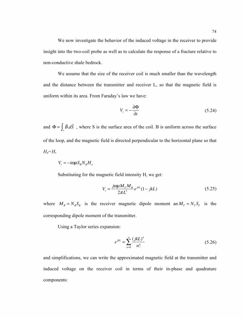
74
We now investigate the behavior of the induced voltage in the receiver to provide
insight into the two-coil probe as well as to calculate the response of a fracture relative to
non-conductive shale bedrock.
We assume that the size of the receiver coil is much smaller than the wavelength
and the distance between the transmitter and receiver L, so that the magnetic field is
uniform within its area. From Faraday’s law we have:
(5.24)
and , where S is the surface area of the coil. B is uniform across the surface
of the loop, and the magnetic field is directed perpendicular to the horizontal plane so that
Hn=Hr
Substituting for the magnetic field intensity H, we get:
(5.25)
where is the receiver magnetic dipole moment an is the
corresponding dipole moment of the transmitter.
Using a Taylor series expansion:
(5.26)
and simplifications, we can write the approximated magnetic field at the transmitter and
induced voltage on the receiver coil in terms of their in-phase and quadrature
components:
Vr = − ∂Φ∂t
Φ =
!B
s∫ .d!S
Vr = −iωµSRNRHn
Vr =jωµMTMR
2πL3e jkL (1− jkL)
MR = NRSR MT = NTST
e jkL = ( jkL)n
n!n=0
∞
∑

75
(5.27) InHz ≈
MT
2πL31− 2
3σµωL2
2⎛⎝⎜
⎞⎠⎟
3/2⎛
⎝⎜
⎞
⎠⎟
QHz ≈MT
2πL3σµωL2
2− 23
σµωL2
2⎛⎝⎜
⎞⎠⎟
3/2⎛
⎝⎜
⎞
⎠⎟
InVr ≈µωMTMR
2πL31− 2
3σµωL2
2⎛⎝⎜
⎞⎠⎟
⎛⎝⎜
⎞⎠⎟
QVr ≈µωMTMR
2πL3σµωL2
2− 23
σµωL2
2⎛⎝⎜
⎞⎠⎟
3/2⎛
⎝⎜
⎞
⎠⎟

5.3 Effect of Magnetic Permeability on Fractures
In a uniform non-conducting medium, the magnetic field does not depend on µ,
while the electric field is directly proportional to the magnetic permeability. In a
conductive medium, the magnetic permeability affects the magnetic field, as the skin
effect is characterized by . When the magnetic permeability of a medium is
increased, the interaction between currents in accord with Faraday’s law increases with
the distribution of induced currents at lower frequencies.
The in-phase and quadrature components of the magnetic field, in terms of the
skin effect p, are given by:
(5.28)
(5.29)
(5.30)
L is the instrument length and H0z and B0z are vertical components of the magnetic field
and magnetic induction of the non-conducting medium. The in-phase component of the
emf changes in linear proportion to the magnetic permeability, while the quadrature
component of the induced currents generates an emf that is proportional to the square of
the magnetic permeability. Also, when p is small, we can approximate the in-phase
component of the magnetic induction to InBz =B0z=µH0z, which shows that it is a function
p = (σµω )1/2
QHz = p2H0z =σµωL2
2H0z
InHz = (1−23p2 )H0z
QBz =σµ2ωL2
2H0z
InBz = B0z −23p2B0z

77
of µ only and practically does not depend on the conductivity of the medium. This
behavior is even more true for short probes, and it is therefore appropriate to use short-
induction probes to reduce the influence of the conductivity of the medium. When the
parameter p is not small and the permeability approaches two, both the in-phase and
quadrature components are affected by σ and µ. However, in measuring the amplitude of
the secondary field, the influence of the magnetic permeability increases. Figure 5.2
shows the effect of increasing permeability on the magnetic field for a case of a
permeable sphere as an example of effect of permeability.
Figure 5-2. Effect of Permeability on Magnetic Field on a Permeable Sphere (r=9cm)

78
5.3 Magnetic Dipole in Two-Layer Permeability Materials
We consider a wellbore of cylindrical shape with a transmitter and receiver located
along the borehole axis in a gas well, as shown in Figure 5.3. The layers of the cylinder
are made of two materials with different permittivities and permeabilities.
Figure 5-3: Two-Layer Medium with Transmitter and Receivers
Using Maxwell’s equations for the quasistationary fields E!"
ejwt and H!"!
ejwt , given
as:
∇× E!"= − jωµH
!"! (5.31)
∇× H!"!
=σ E!"
(5.32)
∇⋅E!"= 0 (5.33)
∇⋅H!"!
= 0 (5.34)
and from vector identity ∇⋅(∇×!A) = 0 , using equation (5.33) we have :

79
!E = − jωµ∇×
!A (5.35)
!A is the vector potential of magnetic type. Substituting Eqn. (5.35) into Eqn.
(5.31), we obtain,
!H = ∇×∇×
!A = ∇∇⋅
!A −∇2 !A (5.36)
Using vector identity, we have,
∇∇⋅A!"−∇2A!"="H (5.37)
We can also use Eqn. (5.32) to write as,
∇×!H = − jωµσ∇×
!A = k2∇×
!A (5.38)
and using vector identities, we can write Eqn. (5.38) as,
H = k2!A −∇φ
We apply the gauge condition to obtain the vector potential Helmholtz equation:
φ = −∇⋅!A (5.39)
∇2 !A + k2
!A = 0 (5.40)
Solving for A!"
, we can obtain the components of the electromagnetic field:
E!"= − jωµ∇× A
!" (5.41)
H!"!
= k2A!"+∇∇⋅A
!" (5.42)
where k2 = − jωµσ .
Since the borehole is of a cylindrical geometry, we choose the cylindrical coordinate
systems (r,φ,z) to write the Helmholtz equation in the form:
1r∂∂r
r ∂A!"
∂r⎛⎝⎜
⎞⎠⎟+ 1r2
∂2A!"
∂φ 2+ ∂2A!"
∂z2+ k2A = 0 (5.43)

80
If the moment of the magnetic dipole is oriented along the z-axis, we would look
for a solution using only the z-component of the vector potential, Az such that:
∇2Az + k2Az = 0 if
The fields of the vector potential and all its components are independent of the φ
coordinate due to symmetry.
The solution of the Helmholtz equation is a product of two functions by separation of
variables: Az = P(r)Φ(r) that must satisfy the following conditions:
Az tends to the vector potential of the magnetic dipole in a uniform medium near
the origin of the coordinate systems of the function, i.e.,
Az(0) = Me− jk1r
4πR if R = (r2 + z2 )1/2 → 0 , M is the dipole moment.
As the distance from the magnetic dipole increases, the vector potential function
tends to be zero.
The tangential components of the electric and magnetic fields are continuous at
the boundaries of the different layers. The magnetic field has two components and
the electric field has one:
Hr =∂2Az∂r∂z
Hz = k2Az +
∂2Az∂z2
Eφ = − jωµ ∂Az∂r
The boundary conditions to be satisfied at the interface are for the above equations:
r2 + z2 ≠ 0

81
kn2Az +
∂2Az,n∂z2
= kn+12 Az,n+1 +
∂2Az,n+1∂z2
µn∂Az,n∂r
= µn+1∂Az,n+1∂r
(5.44)
Based on the uncoupled nature of the solution for the partial differential equation,
we can write the Helmholtz equation as:
(5.45)
and
(5.46)
, λ is the variable of separation.
Solutions for Eqn. (5.46) are functions of sinλz and cosλz, while solutions of the
second equation are modified Bessel functions of zero order, Io(ym) and Ko(ym),
and . The field is symmetric with
respect to z=0, and so the vector potential within the borehole can be written as:
(5.47)
we can use the relationship:
, as
to write:
d 2Φ(z)dz2
+ λ 2Φ(z) = 0
d 2P(y)dz2
+ 1ydT (y)dy
−T (y) = 0
y = (λ 2 + jχ )1/2 r
ym = (λ 2 + jχm )1/2 r = λmr = λmr, λm = (λ 2 + jχm )
1/2
A1* = M
4πe− jk1r
r+ 2π
C1I0 (λ1r)cosλzdz0
∞
∫⎛⎝⎜
⎞⎠⎟
e− jk1r
r= 2π
K00
∞
∫ (λ1r)cosλzdz
K0 (λr)→∞ r→ 0

82
(5.48)
where D1=1.
The general case for n:
(5.49)
where n = 1, 2, ..p.
Eqn. (5.49) contains 2p unknown coefficients at the right-hand side Cn and Cd. We
consider a three-layer medium, namely the internal one, the borehole (ρ1, µ1), the
intermediary part, the fracture invasion (ρ2, µ2) and the outer medium (ρ3, µ3). Using the
boundary conditions from Eqn. (5.44), we can write [21]:
(5.50)
Near the source, inside the borehole where the dipole is located, the coefficient D1
is equal to unity, while in the external medium, the fields must vanish. As the distance r
approaches infinity, I0(λnr) grows exponentially; therefore, the only way for the field to
vanish is that Cn must be zero.
We need to solve for C1 from the equations above to obtain the expression of the
fields inside the borehole. C1= Det1/Det., where Det. is the determinant of the system of
equations.
(5.51)
Az,1* = M
2π 2 C1I0 (λ1r)+ D1K0 (λ1r)[ ]0
∞
∫ cosλzdz
Az,n* = M
2π 2 CnI0 (λnr)+ DnK0 (λnr)[ ]0
∞
∫ cosλzdz
λ12I0 (λ1a1)C1 + λ1
2K0 (λ1a1)− λ22I0 (λ2a1)C2 − λ2
2K0 (λ2a1)D2 = 0λ22I0 (λ2a2 )C2 + λ2
2K0 (λ2a2 )− λ32I0 (λ3a2 )C3 − λ3
2K0 (λ3a2 )D3 = 0
Det1= [−µ1λ1λ22I0 (λ2a1)K1(λ1a1)− µ2λ2λ1
2K0 (λ1a1)I1(λ3a1)][µ2λ2λ3
2K1(λ2a2 )K0 (λ3a2 )− µ3λ3λ22K0 (λ2a1)K1(λ3a2 )]
+[µ1λ1λ22K0 (λ2a1)K1(λ1a1)− µ2λ2λ1
2K0 (λ1a1)K1(λ2a1)][−µ2λ2λ3
2I1(λ2a2 )K0 (λ3a2 )− µ3λ3λ22I0 (λ2a2 )K1(λ3a2 )]

83
(5.52)
If it is a two-layer medium with different permeabilities µ1 and µ2, the function C1
can be obtained from simplifying the above equations:
(5.53)
where:
The components of the electromagnetic field within the borehole can be written as:
Hr = H0r −M4π
2π
λλ10
∞
∫ C1I1(λ1r)sinλzdλ (5.54)
Hz = H0z −M4π
2π
λ12
0
∞
∫ C1I0 (λ1r)cosλzdλ (5.55)
Hφ = H0φ −jµω4π
2Mπ
λ10
∞
∫ C1(λ1r)cosλzdλ (5.56)
H0r , H0z ,, and E0φ are components of the field in a uniform medium with
conductivity σ1.
On the borehole axis Hr =Hφ = 0 and
Hz = H0z −M4π
2π
λ12
0
∞
∫ C1 cosλzdλ (5.57)
Det = [−µ1λ1λ22I0 (λ2a1)I1(λ1a1)+ µ2λ2λ1
2I0 (λ1a1)I1(λ2a2 )][µ2λ2λ3
2K1(λ2a2 )K0 (λ3a2 )− µ3λ3λ22K0 (λ2a2 )K1(λ3a2 )]+
[µ1λ1λ22I1(λ1a1)K0 (λ2a1)+ µ2λ2λ1
2I0 (λ1a1)K1(λ2a1)][−µ2λ2λ3
2I1(λ2a2 )K0 (λ2a2 )− µ3λ3λ22I0 (λ2a2 )K1(λ3a2 )]
C1 =µ1λ2K0 (λ2a)K1(λ1a)− µ2λ1K0 (λ1a)K1(λ2a)µ1λ2K0 (λ2a)I1(λ1a)+ µ2λ1I0 (λ1a)K1(λ2a)
λ1 = (λ2 + jχ1)
1/2 χ1 =σ 1µ1ω
λ2 = (λ2 + jχ2 )
1/2 χ2 =σ 2µ2ω

84
Let us consider:
(5.58)
(5.59)
Using the simplification above and the recursive relations of the Bessel functions
for I0 , which applies to K1 and K2, we can write:
(5.60)
The quadrature component of the magnetic field, expressed in terms of the
primary field, is:
(5.61)
where . We introduce and , the geometric factor, and rewrite
Eqn. (5.61) as:
(5.62)
We can further simplify the expression to:
λ1 = (λ2 + k1
2 )1/2 = λ(1+ k12
λ 2 ) ≈ λ + 12k12
λ
λ2 = (λ2 + k2
2 )1/2 = λ(1+ k22
λ 2 ) ≈ λ + 12k22
λ
I0 (λa) = I0 (λa +12k12aλ) = I0 (λa)+
12k12
λI0' (λa)
I0' (x) = −I1(x)
Iv−1(x)− Iv+1(x) =2vxIv(x)
Iv−1(x)+ Iv+1(x) = 2Iv' (x)
λ12C1 = j(χ2 − χ1)
λa2
2K0 (λa)K1(λa)− λa(K12 − K0
2 )⎡⎣ ⎤⎦
Qhz =σ 1µωL
2
2+ L
3
π(s1 −1)χ1
λa20
∞
∫ [2K0K1 − λa(K12 − K0
2 )]cosλLdλ
s1 =µ2µ1
m = λa α = L / a
Qhz =ωµL2
2(σ 1 + (σ 2 −σ 1)
2απ
m20
∞
∫ [2K0 (m)K1(m)−m(K12 − K0
2 )]cosmαdm)

85
where (5.63)
and G1=1-G2.
The functions and depend on the ratio of the magnetic
pemeabilities s and the geometric factor α. The primary magnetic flux is a function of the
permeability, and at the range of small parameters, a density of induced currents is
directly proportional to the flux of this field and conductivity.
Qhz =ωµL2
2(σ 1G1(α , s)−σ 2G2 (α , s))
G2 =2απ
m20
∞
∫ [2K0 (m)K1(m)−m(K12 − K0
2 )]cosmαdm
G1(α , s) G2 (α , s)

86
5.4 Analysis of Response of Instruments in Presence of Fractures
We consider a borehole with its main axis along the Y-axis. A coil-carrying
current, Ic, is shown at the origin lying in the XY plane with its axis along the Z-axis.
Using spherical coordinates, a vertical fracture is shown rotated at an angle α from the
XY- plane.
Figure 5-4: Fracture Cross Section Showing Probes and Induced Currents.
The fracture lies in the X’Y-plane. A circular eddy current loop is also shown.
The point h on the Y-axis in the borehole is where a receiving coil will be placed to
measure the magnetic field at that point. The electric and magnetic fields surrounding the
small coil carrying an electric current are represented by the magnetic dipole, as derived
in section 5.1.

87
(5.64)
η is the impedance of the medium, N the number of turns of in the coil, S the area
of the coil, I the current in the coil, k the wave number, and r, θ, and φ are the unit
spherical vectors. Assuming a quasistatic solution as kr → 0, we can simplify the Eqn.
(5.6) using a Taylor series of the exponential term, and the electric field can be written as:
(5.65)
where k=ω/c = and , ε is the permittivity, µ the permeability of the
medium, and ω is the angular frequency. The electric field can be rewritten as:
(5.66)
In a medium with low conductivity, the eddy currents can be found by using
Ohm’s law:
(5.67)
It is obvious that the magnitude of the eddy currents would be affected when µ >
1, i.e., in permeable materials. The currents also show the same symmetry with respect to
the E- field. We can use the Ampere’s law to obtain the magnetic fields due to the eddy
currents at a receiver location , due to a source transmitter position, :
r!( )E"!
=η NSI4π
− jkre k2
r− jkr2
⎛⎝⎜
⎞⎠⎟sinθa#φ
H
r!( )
" !""= NSI4π
− jkre 2 jkr2
+ 1r3
⎛⎝⎜
⎞⎠⎟ cosθar
# + − k2
r+ jkr2
+ 1r3
⎛⎝⎜
⎞⎠⎟sinθ
⎡
⎣⎢
⎤
⎦⎥aθ#
E(r! )" !""
= − j kηNSI sinθ4πr2
aφ#
ω µε η = µ / ε
Er
!"!= − j µωNSI sinθ
4πr2aφ#
J!"=σ E!"
r!
r!′

88
(5.68)
Given the arbitrary angle α between the plane of the coil and plane of the eddy
current loop in Figure 5.4, we can obtain the responses of the receiver coil due to the
presence of the fracture. The single coil may be considered using superposition principles
as a sum of two perpendicular coils. We choose the equivalent coils so that one lies in
X’Y plane and the other in XZ’ plane and represent the magnetic moment as:
(5.69)
We can represent the magnetic dipole into the two components:
(5.70)
The electric field around the eddy current loop is similar to equation 5.14, where
θ is measured from the coil’s Z’-axis:
Since the total resistance of the loop is R, the current in the loop given by Ohm’s
law, is:
(5.71)
(5.72)
Applying Ampere’s law to find the magnetic field at a point on the Y-axis, a
length h from the origin due to symmetry, we would have the field in the form:
H!"!
r =14π
I(r ')dl × ("r − "r ')"r − "r ' 2v∫
!M = NSIaz
!M = NSI(cosα aZ ' + sinα aX ' )
!E(!r ) = − j µωNSI cosα
4πr2aφ '
I =
!E.d!l∫
R
I = − j µωNSI cosα2R
!H = IoF(r,h)cosα aZ '

89
F(r,h) is a function of variation with respect to r and h. The angle α determines
the magnitude of the eddy currents and hence the magnitude of the magnetic field. If the
field is measured at h using a small receiver coil of n turns and area s, the voltage induced
will be:
(5.73)
With the two-coil system, the response is determined by , which is at its
maximum when the coils are lined up with the fracture and at its minimum when they are
perpendicular to the fracture. Therefore, as the coils are rotated together, a null would
indicate that the coils are perpendicular to the fracture; conversely, a maximum would
indicate that the coils are in the plane of the fracture. This would enable us to determine
the direction of propagation of the fracture in the shale. In addition, the magnetic material
in the fracture would “amplify” the eddy currents in the fracture so that the depth of the
fracture can be estimated.
We consider a series of N fractures that individually provide received signal strengths
of Vi. If the fractures are embedded in a nonconductive medium like a shale, and the eddy
currents in each fracture are small (low or moderate conductivity) so that the eddy current
distribution in each fracture is unaltered then the total signal is the sum of the signals due
to each fracture being considered separately and using superposition can be expressed as:
(5.74)
where βI is the angle of the ith fracture. The response can be rewritten in the form:
V = −n dφdt
V = − jwnsIoF(r,h)cos2α
V =Vo cos2α
cos2α
V (α ) =V1 cos2(α − β1)+V2 cos
2(α − β2 )+!+VN cos2(α − βN )

90
(5.75)
where
(5.76)
(5.77)
and
(5.78)
The fine structures of a multiple-fractured system cannot be resolved based on the
equation above. For example, for two fractures of equal individual response, the
instrument will have a maximum response when the two coils bisect the angle between
the two fractures.
5.5 Numerical Method for Analysis of Complex Fractures
The Finite Element Method (FEM) provides geometric flexibility to model
complex structures and the capability to model high contrasts in material properties. For
example, Finite Difference meshes are rectilinear and produce staircase-type
(FE) method is used to solve the governing Maxwell diffusion equations, which express
the behavior of the fields in the fractures. The FE analysis algorithm enables local mesh
V (α ) = ′C + ′V cos2(α − ′β )
′C = − ′V2 +
Vi2
i=1
N
∑
′V = Vi cos2βii=1
N
∑⎛⎝⎜⎞⎠⎟
2
+ Vi sin2βii=1
N
∑⎛⎝⎜⎞⎠⎟
2
′α = 12 tan−1
Vi sin2βii=1
N
∑
Vi cos2βii=1
N
∑
⎛
⎝
⎜⎜⎜
⎞
⎠
⎟⎟⎟

91
, which discretize the fractures into an unstructured grid. This allows the
element edges to coincide with the boundaries of irregular fracture inhomogeneities and
allows for
permeability contrasts in the model.
We employ the Finite Element Method (FEM) with vector edge basis functions to
find solutions of the governing diffusive differential equations for the model. Using
coupled-potential formulation for the vector potential gives rise to an ungauged curl-curl
vector potential equation, which when we apply normal FE techniques using nodal basis
functions leads to stiffness matrix with poor condition number [26]. It has been shown
that the vector edge basis [27] provide improved matrix conditioning and a good
representation of material discontinuities that satisfy the tangential boundary conditions
of the fields [58].
The edge-based finite element technique is used in this case to solve the coupled
system of partial differential equations from the formulation. The method converts the
strong to the weak formulation and discretizes the solution domain using tetrahedral
meshes that allow local refinement as implemented in [59]. Homogeneous Dirichlet
boundary conditions are applied at the outer mesh boundaries to truncate the solution
domain. We follow the procedures for implementing the FE methods as outlined in [60]:
Choose proper interpolation functions (otherwise known as shape
functions or basis functions).

92
deriving the weak formulation of the partial differential equation subject to
a set of boundary conditions.
Form the global matrix system of equations through the assembly of all
elements.
Impose Dirichlet boundary conditions.
Solve the linear system of equations using linear algebra techniques.
Post-process the results to obtain desired parameters.
5.5.1 Finite Element formulation for Fractured Shale Medium
At low frequencies, we can neglect the displacement currents and use only the
diffusive form Maxwell’s equations as expressed. We use the gauged EM potentials
formulation [61] and impose the Coulomb gauge condition ∇⋅!A = 0 to ensure that
computed EM potentials do not contain purely divergent spurious modes.
We consider the formulation by [62], where the responses of prescribed shale
homogenous background models or layered earth for the primary potentials ( !Ap ,φp) are
known in closed-form solution. We are interested in using superposition theory of the
fracture response ( A!"s , φs) such that the total response is:
A!"= A!"
p + A!"s
φ=φp+φs

93
Using the same approach to express the fields, we can similarly decompose the
conductivity and permeability into those fields for the cases of with and without fracture
(background model) as follow:
We introduce a parameter referred to as the magnetic reluctivity (v=1/µ), [61], so
that we can write the diffusive form of the Maxwell’s equations as follows.
∇× (ν∇×!A)+σ ( jω
!A −∇φ) =
!J (5.79)
where J is the magnetic dipole current of the transmitter in the borehole.
It is well known [63] that discretization of curl-curl equations leads to asymmetric
finite element matrices and the introduction of numerically unstable spurious modes. The
Biro’s approach [61] incorporates the term −∇(∇⋅A!") to the left side of eqn. (5.79) to
mitigate the problems, which leads to:
∇× (ν∇×!A)−∇(∇⋅
!A)+σ ( jω
!A −∇φ) =
!J (5.80)
The fields due to the primary potentials of the background shale medium due to a
transmitting magnetic dipole satisfy the equation:
∇× (ν p∇×!Ap )+ jωσ p
!Ap +σ pφp =
!Jp (5.81)
The secondary potentials due to the presence of the fracture using the approach
described in [28] are therefore expressed as:
∇× (ν∇× A!"s )+ jσω A
!"s +σ∇φs = −∇× (ν s∇× A
!"p )− jσω A
!"p −σ s∇φp (5.82)
µ = µp + µs
σ =σ p +σ s

94
Next, we satisfy the divergence-free condition ∇⋅!J = 0 , which is not satisfied in
Eqn. (5.81), by introducing an auxiliary equation:
∇⋅!J = ∇⋅(σ
!E) = 0 (5.83)
−∇⋅σ ( jω A!"+∇φ) = 0 (5.84)
We can define the primary and secondary potentials due to Eqn. (5.84) as:
∇⋅σ ( jω A!"s +∇φs ) = ∇⋅( jωσ s A
!"s +σ∇φp ) (5.85)
The primary potentials ( A!"
p , φp) for the fracture analysis are chosen to be those of the
magnetic dipole in a cylindrical medium, which are discussed in section 5.3. They can be
numerically solved for as shown in [36]. It should be noted that the primary potentials
could be responses that may be obtained from a heterogeneous conductivity structure that
may not be solved analytically.
The source for the secondary potentials due to the presence of the fracture is
introduced by the defined primary potentials instead of the direct source current density
!Js due to the transmitting source dipole. The dipole can be of arbitrary shape and
orientation in the formulation based on primary potentials.
It is assumed that the problem is formulated in the cylindrical geometry with an
infinitesimal magnetic dipole located on the Z-axis of the cylindrical solution domain V,
and the outer curved walls of the cylinder and top and bottom caps of the cylinder
constitute the outer boundary S. It is assumed that S is located at a distance such that the
transmitter signals have negligible value, satisfying the Dirichlet boundary condition:
(!As ,φs ) ≡ (0,0) on S (5.86)

95
We apply the Galerkin approach similar to [65] to the boundary value problem of
eqn. (5.82) and (5.85) with vector weighting function !W , and with scalar weighting
functions T, so that the vector potential is expressed as:
A!"s (r) = ai
i=1
M
∑"Wi (r) (5.87)
ai are the scalar coefficients to be determined, and Wi are weighting function vectors of
the edge type. !Wi are important in finding EM solutions by imposing the tangential
!E and
normal !B continuity boundary conditions at interfaces of media smoothly. M is the
number of vector edges obtained from the discretization of the structure using tetrahedral
mesh [64].
The scalar potential is expressed in terms of the nodal basis function T:
(5.88)
The bk are scalar coefficients associated with the nodal basis function that needs to
be obtained. N represents the nodes of the tetrahedral meshes from the discretization.
Using Wi as the test function in the Galerkin formulation for Eqn. (5.82),
!WjV∫ ∇ ×ν∇× ai
i=1
M
∑!WidV +
!WjV∫ jωσ ai
!WdV +
!WiV∫
i=1
M
∑ σ∇ bkTkk=1
N
∑ dV
= −!WjV∫ (∇×ν s∇×
!Ap + jωσ s
!Ap +σ s∇φs )dV
(5.89)
Introducing the divergence theorem using the approach described [61] and the
notation (x,y)V=∫v (xy) dV, reduces the strong formulation of the second-order equation to
a weak-formulation first-order equation:
(!Wj ,∇×ν∇×
!Wi )V = (ν∇×
!Wi ,∇×
!Wj )V − ν∇×
!Wi , n ×
!Wj s
(5.90)
φs (r) = bkk=1
N
∑ Tk (r)

96
Here means a surface integral over S. It vanishes when the Dirichlet boundary
conditions are applied. Rewriting in terms of primary electromagnetic fields ( E!"
p , B!"
p ):
aii=1
M
∑ (∇×!Wj ,ν∇×
!Wi )V + ( jωσ
!Wj )V⎡⎣ ⎤⎦ + bk
k=1
N
∑ (σ!Wj ,∇Tk )V
= −(∇×!Wj ,ν s B
"!p )V + (
!Wj ,σ s E
"!p )V
(5.91)
Similarly, Eqn. (5.84) is also expressed using scalar test function Ti to obtain its
weak form:
− Tj ,∇⋅ jωσ ai
!Wi +σ∇ bkTk
k=1
N
∑i=1
M
∑⎡⎣⎢
⎤⎦⎥
⎛⎝⎜
⎞⎠⎟V
= −(Tj ,∇⋅σ s E"!
p )S (5.92)
Using the vector identity:
(Tj ,∇⋅σ∇
!Wk )V = −(σ∇Tj ,∇
!Wk )V + σTj , n.
!Wk (5.93)
It is also possible to rewrite:
Tj ,∇⋅ jωσ
!Wj( )V = −( jωσ∇Tj ,
!Wj )+ jωσTj , n ⋅
!Wi s
(5.94)
so that the main equation is written as:
aii=1
M
∑ ( jωσ∇Tj ,!Wi )V + bk
k=1
N
∑ (σ∇Tj ,∇Tk )V = −(σ s∇Tk ,E"!
p )V (5.94)
The equations (5.91) and (5.94) form a coupled, weak formulation of the diffusive
equation of electromagnetic waves in terms of the ungauged potentials. Using the Open
Source Finite Element Library, NGSolve [23], the equations are assembled in to linear
algebraic form by implementing integration of the functions (dot products). The systems
of equations are of linear from:
Fu = g (5.2)
x, y S

97
The left-side is the stiffness matrix F. It is complex, symmetric and sparse and is
assembled by analytically computing the inner products using the tetrahedron method and
the right side using method of 14-point quadrature coefficients in [66] and
implementations in [23]. We use an open-source Finite Element Library for the
procedure. The advantage of the NGSolve library is that it is easy to implement the Finite
Element Method, and it is connected to an automatic 3D tetrahedral mesh generator,
NETGEN [18], that is capable of mesh refinement. NGSolve is written in C++ and is
open source [23].
Some features implemented in NGSolve include:
Elements of arbitrary order for any shape (segments, triangles,
quadrilaterals, tetrahedrons, prisms, pyramids, hexagons, etc.)
Scalar elements and vector-valued elements for H(curl) and H(div)
formulations
Integrators for Maxwell’s equations, etc.
Iterative solvers: e.g., Conjugate Gradient Method, with multigrid and
preconditioning techniques
Error estimators and adaptive mesh refinement
Intensively object-oriented C++ language
The geometry of the fracture was designed to resemble a possible fracture [7, 8]
that may occur during the fracturing of a gas well, as shown in Figure 5.6, and the
material proppant effective medium using Bruggeman law was used to fill it.

98
Figure 5-6: The PKN Fracture Model
The parameters for the fracture geometry are:
Shale: Permittivity: 15, Permeability: 1, Conductivity: 0.1 S/m Limestone: Permittivity: 8, Permeability: 1, Conductivity: 0.01 S/m Fracture fracking fluid: Permittivity: 80, Permeability: 2, Conductivity: 0.01 S/m,
Magnetic loss tangent: 0.01 Width Wf: 0.1m, Height hf=0.15m, Depth to be determined.

99
Figure 5-7: Hydraulic-fractured well arrangement showing shale, with cross section of horizontal well with a vertical fracture.
Simulations were performed at a frequency of 500Hz for different fracture depths
to observe the scattered fields due to the presence of a fracture as shown in Fig. 5.7.
Figure 5-8: Relationship between scattered Magnetic fields and fracture depths for a given fracture geometry

100
The scattered electric fields from fractures of the lengths 4m and 12m are plotted
below, showing the difference is scattered fields due to the height difference of the
fractures.
Figure 5-8: Scattered electric fields due to fractures of different lengths
It can be seen from Figure 5.8 that it becomes difficult to estimate the fracture as
the depth increases because scattering is reduced.
5.6 Conclusions
In this chapter we have studied the behavior of magnetic dipoles located in
different media, and have carried out the analysis of their response in the presence of
fractures. We have examined the effect of magnetic permeability when smart proppants
are introduced in a fracture. We have presented an approach for detecting the fracture
0 0.1 0.2 0.3 0.4 0.5 0.6 0.7 0.8 0.9 10
0.05
0.1
0.15
0.2
0.25
0.3
0.35
0.4
points distance (2m)
Ex (V
/m)
4m Frac12m Frac

101
orientation for the case where the fracture orientation is unknown. We have presented a
finite element method, based on an open source finite element library, which is capable of
solving magneto-quasistationary electromagnetic problems. We have shown that for a
given fracture geometry, it is possible to use its properties to estimate its depth based on
scattered fields from the fracture. This would enable us to estimate the depths of the
fractures from measurements made at the fracture openings of the horizontal well.
102
Chapter 6
Conclusions and Recommendations for Further Research
6.1 Conclusions
We can use the version of the Dipole Moment Method developed in Chapters 2
and 3 to study scattering behavior of objects. The objects studied can be either single or
multiple objects in two or three dimensions. A scatterer can be replaced by its equivalent
dipole moments, and once that is done, one is able to obtain the scattered electromagnetic
fields at any distance from the scatterer and at all frequencies, including low frequencies.
The approach was used in studying scattering of particles that can be used as smart
proppants. We introduced Monte Carlo probability distribution techniques to determine
the position of particles in constant position so as to take into consideration their spatial
variations.
The limitations of the Dipole Moment approach were highlighted and the theory
of mixing rules was explored in finding an equivalent medium representation of Magnetic
proppant particles in a hydraulic fracture. There are several mixing rules to choose from,
and at volume inclusions of less than about 20%, any of the three major mixing rules—
Maxwell Garnett, Bruggeman, and Coherent Potential—gives about the same effective
permeability or permittivity of a material. However, as the percentage of inclusions goes
up to about 40%, there are differences. We compared the Dipole Moment approach with
Monte Carlo to the three mixing rules to see that the Bruggeman Mixing rule is closest to
the results of the Dipole Moment approach with the Monte Carlo approach. The Dipole

103
Moment approach may serve as a guide in picking mixing formulas since it gives the full
solution, taking into consideration all statistical variations.
The thesis then delved into use of Magnetic Dipoles as transmitting antennas and
possible responses that can be obtained in the well bore. A procedure for understanding
fracture orientation was highlighted for a situation where there is no idea of the fracture
propagation during the drilling operation.
A low-frequency, forward-modeling, Finite Element Method was implemented
that can model complicated fracture geometry. The magneto-quasistatic Maxwell
equations were used because of the modeling frequencies of 500 Hz or lower. Extremely
low frequencies of operation would be needed to investigate into deeper target fractures
because of the lossy nature of materials in fractures and the shale background. The
forward modeling serves two purposes: it gives us the necessary synthetic data for
studying the inverse problem, and it provides an understanding of the fracture problem
and its response to electromagnetic stimulation. A numerical modeling of a fracture was
done to estimate depths with varying fracture length. The source operating frequency,
fracture geometry, and materials play a significant role in the ability to estimate effective
depth.
6.2 Recommendation for Future Work
In using probability techniques with the Dipole Moment approach, it was found
that the matrix problem size increases exponentially, and the Monte Carlo approach
becomes even more complex. It may be possible to explore this issue using quasi-Monte

104
Carlo techniques that are shown to have quick convergence and may handle bigger
problems.
Major investigations of mixing rules were limited to only three of the formulas.
There are several other formulas available in the literature. It is possible to use the Dipole
Moment Approach with statistics to aid in understanding their accuracy in finding
effective medium properties of materials with different inclusion volumes.
A study of other possible complex fracture geometries can be carried out with
different material properties to increase the possibility of investigating deeper depths of
the fractures. The work carried out here consists of only the analysis; there is need to
practically test this approach in real-life environments using the magnetic materials
already manufactured.
The study focused on the forward modeling of the fracture at low frequencies, and
there is need to develop numerical inversion techniques for the inverse problem of the
depth estimation at multiple frequencies. The study here is based on back-scattered fields
with source and receivers located in the same borehole. Given the scenario where there
are quite a few drilled wells already, it is possible to do cross-hole, source-receiver
configuration studies for magnetic proppant particles that may increase the capability of
handling larger depth of investigation.

105
Bibliography
[1] http://www.eia.gov/naturalgas/ US natural gas production, visited May, 7, 2014 [2] Zhou, Q, Audio-Frequency Electromagnetic Tomography for Reservoir
Evaluation, Lawrence Berkeley lab., CA, October,1989 [3] Serra, O., Fundamental of well-log interpretation: Developments in Petroleum
Science, Elsevier Science Publishers, Amsterdam, The Netherlands, 1988 [4] King, G.E. 2012. Hydraulic Fracturing 101: What Every Representative,
Environmentalist, Regulator, Reporter, Investor, University Researcher, Neighbor and Engineer Should Know About Estimating Frac Risk and Improving Frac Performance in Unconventional Gas and Oil Wells. Paper SPE 152596 presented at the 2012 SPE Hydraulic Fracturing Technology Conference, The Woodlands, Texas, 6-8 February.
[5] Jechumtálová, Z., Eisner, L. 2008. Seismic source mechanism inversion from a
linear array of receivers reveals non-double-couple seismic events induced by hydraulic fracturing in sedimentary formation. Tectonophysics 460: 124-133.
[6] Cipolla, C.L., Wright, C.A. 2000. Diagnostic Techniques to Understand
Hydraulic Fracturing: What? Why? and How? Paper SPE 59735 presented at the 2000 SPE/CERI Gas Technology Symposium, Calgary, Alberta, Canada, 3-5 April.
[7] Nordgren, R. P. 1972. Propagation of a vertical hydraulic fracture. Soc. Pet. Eng.
J. 12:306–314 [8] Perkins, T. K., and Kern, L. R. 1961. Widths of hydraulic fractures. J. Pet. Tech.
13:937–949. [9] Gao, G., Alumbaugh, D., Zhang, P., Zhang, H., Levesque, C., Rosthal, R., Liu, J.,
Abubakar, A., Habashy, T. 2008. Practical implications of nonlinear inversion for cross-well electromagnetic data collected in cased-wells. Presented at the 2008 Annual Meeting of the Society of Exploration Geophysics, Las Vegas, Nevada, 9-14 November.
[10] Gao, G., Alumbaugh, D., Chen, J., Eyl, K. 2007. Resolution And Uncertainty Analysis for Marine CSEM and Cross-well EM Imaging. Presented at the 2007 Annual Meeting of the Society of Exploration Geophysics, San Antonio, Texas, 23-28 September.

106
[11] Pardo, D., Torres-Verdin, C. 2011. Sensitivity study to quantify hydrofractures with borehole resistivity measurements. Presented at the 11th Annual Meeting of the Joint Industry Research Consortium on Formation Evaluation, University of Texas at Austin, Austin, Texas.
[12] O. F. Mossotti. Discussione analitica sull'inuenza che l'azione di un mezzo
dielettrico ha sulla distibuzione dell'elettricita alla super_cie di piu corpi elettrici disseminati in esso. Memorie di Matematica e di Fisica della Societa Italiana delle Scienze, 24(2):49-74, 1850.
[13]
undVerlag von Friedrich Vieweg und Sohn, Braunschweig, Germany,1879. [14] Lord Rayleigh (J. W. Strutt). On the influence of obstacles arranged in rectangular
order upon the properties of a medium. Philosophical Magazine, 34(1892):481-502,1892.
[15] Lord Rayleigh (J. W. Strutt). On the incidence of aerial and electric waves upon
small obstacles in the form of ellipsoids or elliptic cylinders, and on the passage of electric waves through a circular aperture in a conducting screen. Philosophical Magazine, 44:28{52, 1897.
[16] J. C. Maxwell Garnett. Colours in metal glasses and in metallic _lms.
Philosophical Transactions of the Royal Society of London. Series A, 203:385{420, 1904.
[17] R. E. Kleinman, “The Rayleigh Region,” Proceedings of the IEEE Vol 53, pg
848- 856, 1965 [18] R. E. Kleinman, “Dipole Moments and Near Field Potentials,” Appl. Sci. Res. 27,
April 1973 [19] J. B. Keller. Conductivity of a medium containing a dense array of perfectly
conductingspheres or cylinders or nonconducting cylinders. Journal of Applied Physics, 34(4):99 1993, 1963.
[20] Elliott, R.J., Krumhansl, J.A., and Leath, P. I., “The theory and properties of randomly disordered crystals and related physical systems”, Reviews of Modern Physics, July 1974, 46, (3), pp. 465-543
[21] Kaufman, A. and Dashevsky, Y.A., Principles of Induction Logging, Elsevier,
2003 [22] D. R. Smith, S. Schultz, P. Markos, and C. M. Soukoulis. Determination of
effective permittivity and permeability of metamaterials from reflection and

107
transmission coefficients. Physical Review B, 65(19):195104, Apr 2002. [23] Joachim Schöberl, NGSolve Finite Element Library
http://sourceforge.net/projects/ngsolve/ : visited on February 2, 2014 [24] Grant, F.S., and G.F. West, 1965, Interpretation Theory in Applied Geophysics:
McGraw–Hill.
[25] Qiushi Chen; Konrad, A, "A review of finite element open boundary techniques for static and quasi-static electromagnetic field problems," Magnetics, IEEE Transactions on , vol.33, no.1, pp.663,676, Jan 1997
[26] Biro, O., 1999, Edge element formulations of eddy current problems: Computer
Methods in Applied Mechanics and Engineering, 169, 391–405. [27] Sugeng, F. and A. Raiche, 2004, Modeling the electromagnetic response in
complex geologic structures using the 3D finite–element method based on the hexahedral and tetrahedral edge element technique: 17th Geophysical Conference and Exhibition, ASEG Expanded Abstracts
[28] John L. Volakis, Arindam Chatterjee, and Leo C. Kempel. Finite Element Method
Electromagnetics: Antennas, Microwave Circuits, and Scattering Applications (IEEE Press Series on Electromagnetic Wave Theory). Wiley-IEEE Press,1 edition, June 1998.
[29] A. Taflove and S. C. Hagness, “Computational Electrodynamics: The Finite-
Difference Time-Domain Method”,3rd edition, Artech House Publishers, 2005. [30] R.E. Kleinman, “Far Field Scattering at Low Frequencies,” Appl. Sci. Res. 18,
Aug. 1967 [31] G. Dassios and R.E. Kleinman, Low Frequency Scattering, Oxford Science
Publications, The Clarendon Press, Oxford University Press, New York, 2000 [32] T.B. A Senior, R.E. Kleinman, “Rayleigh Scattering Cross Sections,” University
of Michigan, Radiation Laboratory, Feb. 1970 [33] R. E. Kleinman, “Dipole Moments and Near Field Potentials,” Appl. Sci. Res. 27,
April 1973 [34] R. F. Harrington, “Time Harmonic Electromagnetic Fields,” McGraw Hills, New
York 1961 [35] R.F. Harrington, “Field Computation by Moment Methods”, Wiley-IEEE Press,
May 1993

108
[36] Hastings, W.K. , "Monte Carlo Sampling Methods Using Markov Chains and Their Applications," Biometrika 57 (1): 97–109, 1970
[37] Ding, K. H. and L. Tsang (1989), Effective propagation constants in media with
densely distributed dielectric particles of multiple sizes and permittivities, in Progress in Electromagnetic Research, PIER 1, (edited by J. A. Kong), Chapter 3, 241-295, Elsevier, New York.
[38] L. Tsang, J.A. Kong, K-.H. Ding, and C.O. Ao, Scattering of Electromagnetic Waves: Numerical Simulations, Chapter 8, Wiley-Inter Science, New York 2001
[39] E. Lucente, A. Monorchio, and R. Mittra, “An Iteration-Free MoM Approach Based on Excitation Independent Characteristic Basis Functions for Solving Large Multiscale Electromagnetic Scattering Problems,” IEEE Trans. Antennas and Propag., vol. 56, pp. 999—1007, April 2008.
[40] R.E. Rosensweig, Ferrohydrodynamics, Dover Publications, 1997
[41] J.B. Jarvis, et al ,“Measuring the Permittivity and Permeability of Lossy Materials: Solids, Liquids, Metals, Building Materials, and Negative-Index Materials,” NIST Technical Note 1536, Boulder CO, 2005.
[42] A. M. Nicolson and G. F. Ross. Measurement of the intrinsic properties of
materials by time-domain techniques. IEEE Transactions on Instrumentation and Measurement,19(4):377-382, November 1970.
[43] W. B. Weir. Automatic measurement of complex dielectric constant and
permeability at microwave frequencies. Proceedings of the IEEE, 62(1):33-36, [48] X. Chen, et al, “Robust method to retrieve the constitutive effective parameters of
Meta materials,” Physical Review E 70, 016608 (2004) [45] D.M. Pozar, Microwave Engineering, Wiley Interscience, 2011 [46] Ari Sihvola. Electromagnetic Mixing Formulas and Applications. IEE
electromagnetic waves series 47. The Institute of Electrical Engineers, London, UK, 1999.
[47] Sihvola, A. H., and I. V. Lindell, “Effective Permeability of Mixtures,” JPIER
Chapter 4, 2006 [48] Sihvola, A. H., and J. A. Kong, “Effective permittivity of dielectric mixtures,”
IEEE Trans. Geoscience. Remote Sensing, 27(1), 101-102, Jan. 1989

109
[49] Hashin, Z., and S. Shtrikman, “A variational approach to the theory of the effective magnetic permeability of multiphase materials,” J. of Applied Physics, 33(10), 3125-3131, 1962
[50] Polder, D., and J. H. van Santen, “ The effective permeability of mixtures of solids,” Physica, XII (5), 257-271, 1946
[51] D. A. G. Bruggeman. Berechnung verschiedener physikalischer Konstanten von heterogenen Substanzen. I. Dielektrizittskonstanten und Leitfhigkeiten der Mischkrper aus isotropen Substanzen. Annalen der Physik, 416(7):636-664, 1935.
[52] De Loor, G.P., “Dielectric properties of heterogeneous mixtures containing water.” The Journal of Microwave Power, 1968, 3, pp. 67-73
[53] Bottcher, C.J.F.: 'Theory of electric polarization' (Elsevier, Amsterdam, 1952)
[54] Tsang, L., Kong, J.A., And Shin, R.T., “Theory of microwave remote sensing,” Wiley, New York, 1985
[55] Kohler, W.E., And Papanicolaou, G.C., “Some applications of the coherent potential approximation', in Chow,P.L., Kohler, W.E., And Papanicolaou, G.C. (Eds.), “Multiple scattering and waves” North Holland, New York, 1981, pp. 199-223
[56] Sihvola, A., “Self-consistency aspects of dielectric mixing theories,” IEEE Transactions on Geoscience and Remote Sensing, 1989, 27, (4), pp. 403-415
[57] Wait, J. R., 1982, Geo-electromagnetism: Academic Press, Inc., p. 140-146.
January 1974. [59] Joachim Shoerbel : Netgen Mesh Generator
http://sourceforge.net/projects/netgen-mesher/ : visited on February 2, 2014 [60] J.M. Jin, The Finite Element Method in Electromagnetics, 2nd ed. Hoboken, NJ:
Wiley, 2002. [61] Biro, O., and K. Preis, 1989, Finite element analysis of 3–D eddy currents: IEEE
Transactions on Magnetics, 25, 3145–3159.
[62] M.E. Everett, et al, “3-D Finite Element Analysis of Induction Logging in a Dipping Formation,” IEEE Trans. on Geo. and Remote Sensing, Vol. 39, No. 10, October 2001
[63] G. Mur and I. E. Lager, On the causes of spurious solutions in electromagnetics, Electrotechnics, vol. 22, no. 4, pp. 357-367, 2002

110
[64] S. Mukherjee, “3D controlled-source electromagnetic edge-based finite element modeling of conductive and permeable heterogeneities”, Geophysics, 76(4): F215, 2011
[65] C Koutschan, C Lehrenfeld, J. Schöberl: Computer Algebra meets Finite Elements: an Efficient Implementation for Maxwell's Equations in: Numerical and Symbolic Scientific Computing: Progress and Prospects, Ulrich Langer and Peter Paule (ed.), pp. 105-122. 2011. Springer, Wien
[66] E. A. Badea, M. E. Everett, G. A. Newman, and O. Biro, “Finite element
analysis of controlled-source electromagnetic induction using Coulomb gauged potentials,” Geophysics, vol. 66, May–June 2001.

111
VITA Muhammed Kabiru Hassan
EDUCATION
Ph.D. Electrical Engineering 2008-2014 The Pennsylvania State University, University Park, Masters of Science, Electrical Engineering 2005-2006 The Pennsylvania State University B. Eng. Electrical & Electronic Engineering (2nd Class Upper Div.)1997-2002 Abubakar Tafawa Balewa University, Bauchi Nigeria EXPERIENCE Research/Graduate Assistant Aug. 2008- May 2013 The Pennsylvania State University Short Term Consultant (Power & Energy) Feb. 2008- Dec 2008 The World Bank Group, Washington DC
R&D Engineering Intern Jan 2007- Dec 2007 Data Communication Competent Center Nexans Corporation, New Holland, USA Electrical Engineer 2003-2004 Gombe State Government Nigeria National Youth Service Corps 2002-2003 National Electric Power Authority, Katsina District, Nigeria