low-field nmr studies of structure and dynamics in
TRANSCRIPT

LOW-FIELD NMR STUDIES OFSTRUCTURE AND DYNAMICS INSEMICRYSTALLINE POLYMERS
Dissertation
zur Erlangung desDoktorgrades der Naturwissenschaften (Dr. rer. nat.)
vorgelegt dem
Institut für Physikder Naturwissenschaftlichen Fakultät II
der Martin-Luther-Universität Halle-Wittenberg
von
Kerstin Schälergeboren am 20. April 1983 in Zwenkau
Halle/Saale, den 06. 11. 2012

Gutachter:
1. Prof. Dr. Kay Saalwächter (MLU)
2. Prof. Dr. Mario Beiner (MLU)
3. Prof. Dr. Siegfried Stapf (TU Ilmenau)
Eröffnung des Promotionsverfahrens: 21. November 2012Öffentliche Verteidigung: 05. März 2013

„Ich will Ihnen das Geheimnis verraten,das mich zum Ziel geführt hat.
Meine Stärke liegt einzig und alleinin meiner Beharrlichkeit.“
Louis Pasteur (1822 - 1895)

Contents
1. Introduction 1
2. Semicrystalline Polymers 4
3. Low-Field Proton Nuclear Magnetic Resonance 83.1. Nuclear Spins and Magnetization . . . . . . . . . . . . . . . . . . . . . . . 83.2. The Free Induction Decay . . . . . . . . . . . . . . . . . . . . . . . . . . . . 93.3. Dipolar Interactions and their Influence on the NMR Signal . . . . . . . 10
4. Low-Field Proton NMR Applications for the Investigation of Semicrys-talline Polymers 144.1. The Free Induction Decay of Semicrystalline Polymers . . . . . . . . . . . 144.2. The Magic Sandwich Echo . . . . . . . . . . . . . . . . . . . . . . . . . . . 204.3. Proton Spin Diffusion in Semicrystalline Polymers . . . . . . . . . . . . . 26
4.3.1. The Spin-Diffusion Experiment . . . . . . . . . . . . . . . . . . . . 274.3.2. The Differential Equation for Spin Diffusion . . . . . . . . . . . . . 28
4.4. NMR Filter Sequences . . . . . . . . . . . . . . . . . . . . . . . . . . . . . . 304.4.1. The MAPE Dipolar Filter Sequence . . . . . . . . . . . . . . . . . . 324.4.2. The Double-Quantum Filter Sequence . . . . . . . . . . . . . . . . 33
5. Dynamics in Crystallites of Semicrystalline Polymers 395.1. Investigation of PCL Crystallite Dynamics on Different Time Scales . . . 395.2. Determination of Chain-Flip Rates in PE Crystallites for Two Different
Sample Morphologies . . . . . . . . . . . . . . . . . . . . . . . . . . . . . . 51
6. Crystallization of PCL 61
7. Investigation of Spin Diffusion in PCL 707.1. Spin-Diffusion Coefficients of Heterogeneous Polymers . . . . . . . . . . . 707.2. Proton Low-Field NMR and SAXS Measurements of Semicrystalline PCL 747.3. Simultaneous Fit of Spin-Diffusion and Saturation-Recovery Data . . . . 807.4. Magnetization Transfer Lags in PCL Spin-Diffusion Experiments . . . . 847.5. Effects of Corrugated Crystalline-Interphase Boundary Surfaces . . . . . 907.6. Quantitative Results from Fitting PCL Spin-Diffusion Data . . . . . . . . 937.7. Initial Rate Approximation for the Estimation of Domain Sizes in PCL . 977.8. Summarizing Remarks . . . . . . . . . . . . . . . . . . . . . . . . . . . . . 101
8. The Influence of Cyclic Chain Topology on PCL Dynamics and Crystal-lization 1038.1. Chain Mobility in the Melt . . . . . . . . . . . . . . . . . . . . . . . . . . . 1058.2. Crystallinity and Crystallization . . . . . . . . . . . . . . . . . . . . . . . . 1108.3. Domain Thicknesses . . . . . . . . . . . . . . . . . . . . . . . . . . . . . . . 1138.4. Summarizing Remarks . . . . . . . . . . . . . . . . . . . . . . . . . . . . . 117
9. Summary 119
A. Experimental Details 123
Dissertation of Kerstin Schäler

A.1. Experimental Techniques . . . . . . . . . . . . . . . . . . . . . . . . . . . . 123A.2. Samples . . . . . . . . . . . . . . . . . . . . . . . . . . . . . . . . . . . . . . 128
B. PCL Degradation Investigations 130B.1. Degradation of Cyclic PCL Chains . . . . . . . . . . . . . . . . . . . . . . . 130B.2. Degradation of Linear PCL Chains . . . . . . . . . . . . . . . . . . . . . . 130
C. Quantum-Mechanical Basics of NMR 132
D. Demonstration of the Effect of Diverse Pulse Sequences 140D.1. Average Hamiltonian Theory for Calculating the Mode of Action of Pulse
Sequences . . . . . . . . . . . . . . . . . . . . . . . . . . . . . . . . . . . . . 140D.1.1. The Magic Sandwich Echo . . . . . . . . . . . . . . . . . . . . . . . 140D.1.2. The Magic and Polarization Echo . . . . . . . . . . . . . . . . . . . 149
D.2. The Double-Quantum Filter . . . . . . . . . . . . . . . . . . . . . . . . . . 150
E. PCL Densities 155
F. Spin Diffusion 156F.1. Description of Magnetization Transfer Between Two Spins 1/2 . . . . . . 156F.2. The Simulation Program for Calculating Spin-Diffusion and Saturation-
Recovery Curves . . . . . . . . . . . . . . . . . . . . . . . . . . . . . . . . . 157F.3. Derivation of the Source Domain Size by means of the Initial Rate Ap-
proximation . . . . . . . . . . . . . . . . . . . . . . . . . . . . . . . . . . . . 158F.4. Effects of PCL Domain-Thickness Distributions on Spin Diffusion . . . . 161
Bibliography 167
Dissertation of Kerstin Schäler

1. Introduction
1. Introduction
Many industrially important polymeric materials are semicrystalline. Their macro-scopic chemical and mechanical properties are governed by the interplay between thewell-ordered crystalline domains and the mobile-amorphous regions, both possessingindividual microscopic features, such as domain geometry or size and chain mobility. Amultitude of experimental techniques is available for the investigation of such heteroge-neous polymer structures, e. g., Small Angle X-Ray and Neutron Scattering (SAXS andSANS), Electron and Atomic Force Microscopy (EM and AFM), Raman and fluorescencespectroscopy or thermal analysis. As Nuclear Magnetic Resonance (NMR) spectroscopyexperiments detect spin interactions in and between molecules, they can provide verylocal information on dynamics and structure and are therefore eminently suited for theinvestigation of semicrystalline polymers.
The beginnings of NMR trace back to studies of Bloch and Purcell et al. who, indepen-dently from each other, detected first NMR signals shortly after the end of the secondworld war. This discovery was rewarded with the Nobel prize for physics for Bloch andPurcell in 1952. At that time, all fundamental parameters influencing the NMR signal,such as the chemical shift, the dipolar splitting, indirect spin-spin couplings, quadrupo-lar couplings and molecular dynamics, have already been known and a general NMRtheory was on hand [1].
During this early years of NMR the measurements based upon the continuous-wavesweep method yielding frequency spectra directly. Yet, the introduction of pulsed NMRby R. Ernst in 1964 in combination with the Fourier transform to generate analyzablespectra from the directly detected time-domain signals represented an important stepforward in the development of NMR spectroscopy, as it brought about a dramatic in-crease in sensitivity of the method [2]. This progress opened up new fields of researchand is the state of the art until today. For his work and his services in two-dimensionalNMR Ernst received the Nobel prize for chemistry in 1991 [1,2].
The shift from high-performance electromagnets to superconducting magnets in the1960s [3] enabled a significant increase in spectral resolution. Since then lots of ad-vancements of NMR techniques have been made with regard to the diverse fields ofapplications, e. g., the development of multiple-pulse sequences, Magnetic ResonanceImaging (MRI) or Pulsed Field Gradient (PFG) NMR and the introduction of Magic-Angle Spinning (MAS) or two-dimensional spectroscopy [1]. To achieve higher sen-sitivity and spectral resolution, magnetic fields of increasing strength are required.Currently, superconducting magnets with proton Larmor frequencies up to 1 GHz areavailable [4]. Yet, such magnets are heavy, bulky, immobile and expensive in purchaseand maintenance. Moreover, the operation of high-field spectrometers is rather com-plex. Another option for an enhancement of the resolution consists in fast Magic-AngleSpinning of the sample in order to average out spin interactions which lead to broadspectral lines [5]. The largest rotation frequencies attainable at present range at about80 kHz [6]. Probe heads and rotors suited for this ultrafast rotation, however, are expen-sive. Nevertheless current trends in solid-state NMR tend toward maximum magneticfield strengths and rotation frequencies [7], leading to highly elaborate, cost-intensiveand interference-prone technology.
Yet, robust and cheap low-field proton NMR may provide valuable insights in structure
Dissertation of Kerstin Schäler Page 1

1. Introduction
and dynamics of semicrystalline polymers. Low-field spectrometers are easy to handlesince they use permanent magnets and comparably simple technology. Admittedly, dueto the weak magnetic field and its rather strong inhomogeneity, chemical resolution can-not be achieved here. Hence, low-field devices are mainly used for standard relaxometryapplications in industry. However, beyond that, they offer the opportunity to investigateproton dipolar couplings, the strength of which does not depend on the magnetic fieldstrength. As the proton dipolar coupling strength is an indicator for segmental dynamicsin polymers, low-field NMR is a suitable method for the investigation of chain dynam-ics, e. g., in crystallites and mobile-amorphous domains of semicrystalline polymers orin polymer melts. Moreover, differences in chain mobility between the individual phasesof a semicrystalline polymer can be observed by low-field NMR, enabling the detectionof crystallinity and domain sizes [8]. Due to the exploitation of an internal mobilitycontrast, a particular sample pretreatment, such as staining, is not required here asopposed to other methods, e. g., EM.
Besides the demonstration of the versatile capabilities of low-field NMR spectroscopyfor the investigation of semicrystalline polymers, the objective of this thesis is the explo-ration of the relation between polymer chain mobility and the semicrystalline structure.For this purpose, two polymer systems, poly(ε-caprolactone) (PCL) and poly(ethylene)(PE) have been investigated by low-field 1H NMR spectroscopy. Despite of their rathersimilar chemical structure they seem to differ in crystallite chain mobility. While PE isan αc-mobile polymer with chains performing helical jump motions within the crystal-lites, PCL is said to be crystal-fixed. As a start, diverse low-field NMR methods had tobe adapted to the application to these polymers, such as
• FID and MSE measurements for the determination of the phase composition,
• spin-diffusion and Saturation-Recovery experiments for the exploration of domainsizes and
• the MSE sequence to study the intermediate-regime chain mobility within thepolymer crystallites.
Hence, after a short introduction regarding semicrystalline polymers and the basics oflow-field NMR in general in Chapters 2 and 3, these NMR methods, which primarilyhave been used for the investigations presented here, are explicated in Chapter 4. Theyhave furthermore been utilized to study diverse specific problems of polymer-physical ormethodological interest:
• The chain dynamics in PCL and PE crystallites has been investigated with regardto the questions whether PCL in fact can be classified as a crystal-fixed polymerand whether the jump rate of the local chain-flip process in PE crystallites dependson the phase morphology (see Chapter 5).
• The crystallization of PCL has been studied in terms of reproducibility of the crys-tallization isotherms measured by low-field NMR (see Chapter 6).
• The method of proton spin diffusion has been established for the determination ofPCL domain sizes by low-field NMR (see Chapter 7).
• The influence of chain topology on chain mobility and the semicrystalline structurehas been explored by comparing linear and macrocylic PCL with regard to meltmobility, crystal growth, crystallinity and domain sizes (see Chapter 8).
Dissertation of Kerstin Schäler Page 2

1. Introduction
The majority of the investigations have been performed by means of low-field Brukerminispec spectrometers with a permanent magnet (field strength B0 ∼ 0.5 T) at a protonLarmor frequency of about 20 MHz. Only for Section 5.1 two high-field NMR techniqueshave been used exceptionally, in order to extend the time range of the dynamics inves-tigations. Moreover, to corroborate the low-field NMR results, complementary methodsof the experimental polymer physics have been applied. Details concerning the experi-mental techniques, settings and samples are given in Appendix A.
Dissertation of Kerstin Schäler Page 3

2. Semicrystalline Polymers
2. Semicrystalline Polymers
Polymers are long chain molecules, mostly hydrocarbons, which consist of many cova-lently-bonded molecular units, named monomers [9, 10]. They are of particular impor-tance in industry and everyday life, e. g., in the form of molded materials, plastic filmsand synthetic fibers. As their macroscopic properties, such as tensile strength, rigid-ity, elasticity, temperature and fatigue resistance, depend on molecular structure anddynamics as well as on the assembly of the chains, investigations of these features areof much interest. Basically, depending on the assembly of the chains, a distinction ismade between purely amorphous and semicrystalline polymers. This work focuses oninvestigations of the latter.
In a polymer melt the chains adopt entangled random-coil conformations with statisti-cally determined backbone bond angles, lacking long-range chain order and thus form-ing liquid-like amorphous material [9]. If the chains exhibit a sufficiently regular chem-ical constitution and linear architecture, the material is able to crystallize at tempera-tures below the melting point by partial disentanglement and stretching of chains. Thestretched chain parts take on helical conformations of minimal intramolecular confor-mational energy and pack parallely into three-dimensional crystalline arrays so as tominmize the packing energy [10]. Here, a crystalline unit cell can be defined similar tothose in anorganic crystals.
The thermodynamic equilibrium state is represented by the extended chain crystal com-prising completely stretched chains. However, the stretching of entangled chains posesan entropic barrier to crystallization. Hence, the evolving structure is not the one withminimum free energy but the one, which forms most rapidly [10]. Entanglements andother topological impurities, such as chemical defects, loops, chain ends, crosslinks orshort chain branches, which cannot be resolved and stretched during the available time,are rejected from the crystallites and concentrated in amorphous regions between them.Thus a semicrystalline structure is formed, usually consisting of lamellae of highly or-dered crystalline material and disordered amorphous domains with almost isotropicchain orientation and high chain mobility in between (see Fig. 2.1) [9, 10]. It is thecombination of characteristics of the crystalline and amorphous phase, which inducesthe rigid but flexible consistency of semicrystalline polymers.
The deformed entanglements within the amorphous phase cause an increase in the freeenergy as compared to the melt and impose a pressure upon the crystalline lamellae,thus stabilizing them at a certain thickness [11]. This thickness in chain direction istypically low, i. e. in the range of 10 nm, while the lateral lamellar extensions are in themicrometer range [9, 10]. The crystalline lamellae arrange themselves in stacks whichform superstructures, such as spherulites [10].
The transition zone between crystalline and amorphous regions was and still is a matterof debate [9, 12–15]. According to Flory the border between the two domains must beless sharp than in monomeric systems, as a portion of the well-ordered chains, whichleave the crystallite, have to disperse into the disordered amorphous phase, where themultitude of possible chain conformations results in a larger space requirement of thesingle chains [13, 16]. Therefore, diffuse interphase regions are formed, with a thick-ness of a few nanometers, which are characterized by partial order and restricted mo-bility of the chain segments as compared to the mobile-amorphous phase [9, 17]. In-
Dissertation of Kerstin Schäler Page 4

2. Semicrystalline Polymers
Figure 2.1.: Arrangement of polymer chains ina lamellar semicrystalline struc-ture with domain thicknesses dc,da and di of the crystalline lamel-lae, mobile-amorphous regions andinterphase regions, respectively.
Figure 2.2.: Chemical structure of poly(ε-capro-lactone) (PCL, upper part) andpoly(ethylene) (PE, lower part).
vestigations of semicrystalline polymers using diverse experimental methods, such as(Time-Modulated) Differential Scanning Calorimetry (TM DSC), dielectric and dynamic-mechanical spectroscopy, in fact militate in favor of the existence of a rigid-amorphousinterphase [15, 18, 19]. The structure of the interphase is affected, e. g., by the freeenergy of chain folds, the chain density at the crystallite surface and the space require-ment of chain segments in the crystalline and amorphous phase and hence is polymerspecific [9,13].
For creating optimized polymer structures profound knowledge of polymer crystalliza-tion is necessary. However, the crystallization process is not clarified completely on amolecular level. It is known, that the crystal growth, proceeding at the lateral faces ofthe lamellae, is a thermally activated process with a barrier in Gibbs free energy, whichhas to be overcome in order to attach chain stems to the growth front. However, thenature of the barrier and its reason remain indistinct [10, 20]. Both, enthalpic [21, 22]and entropic [23,24] barriers are subject of crystallization theories [20]. While the clas-sical model of crystallization kinetics by Hoffman and Lauritzen is based on the as-sumption of a successive, thermally activated attachment of single chain stems to thecrystal growth front, more current multi-stage models presume a pre-arrangement ofchains within a mesomorphic phase, before the actual crystallization takes place [23,25].Other models propose collective local ordering processes of several polymer chains atonce or spinodal-like processes during crystallization [26, 27]. Although certain effectsof molecular weight on domain thicknesses have been proven experimentally [9,28–30],crystallization theories still do not address this topic. Moreover, the influence of chaintopology, the structure of the mobile-amorphous phase (and the interphase) as well asthe role of entanglements prior to and during crystallization is currently under discus-sion [11,31–38].
Besides the phase structure of the polymers also chain dynamics influence the mechan-ical properties. Molecular motions are typically characterized by a correlation time τc,describing an average time required for an orientational change [39], or a motionalrate k ∝ 1/τc. Generally, there is a hierarchy of dynamical processes in polymers, in-cluding very fast subsegmental motions, conformational changes of a few neighboringmonomers, slower cooperative motions of longer chain segments and even motions of
Dissertation of Kerstin Schäler Page 5

2. Semicrystalline Polymers
the whole chain via reptation and free diffusion [10,40,41]. The different motional pro-cesses are usually named α, β and γ according to the order of their emergence in anexperiment, commencing with the process at the highest temperature, i. e. the lowestmotional rate and largest correlation time, respectively. However, the denotation doesnot contain information about the origin of a molecular motion [10,17,42].
Compared to a purely amorphous polymer, the dynamical processes in a semicrystallinepolymer are much more complex and less uniform as a result of the motional restrictionsarising when chains are partially fixed in the crystallites [10,42]. Local processes, suchas side chain motions, take place at high motional rates, i. e. small correlation times. Asin purely amorphous polymers, there is often a distribution of rates, e. g., due to the cou-pling of motions of different side groups [10,17]. Cooperative segmental motions, whichform the basis of the viscoelasticity of polymer melts and lead to the glass transitionwhen freezing in at decreasing temperature, can be found in the amorphous regions ofsemicrystalline polymers as well. They usually exhibit a distribution of motional rates,too. However, in comparison to purely amorphous polymers, the trapping of entangle-ments in the mobile-amorphous domains causes changes in the rate of the segmentalmotions and the temperature dependence of this rate and results in a broadening ofthe rate distribution [10,42]. The motional constraints may even induce new relaxationmodes [10]. Motions of whole chains at low rates, which require chain disentanglementand are known to occur in polymer melts, are usually suppressed in semicrystallinepolymers due to the fixation of the chains in the crystallites [10].
Additional dynamical processes may occur in the polymer crystallites, e. g., microscopicchain diffusion as a result of helical jumps of whole repeat units. Such a motion, aso-called αc process [43, 44], is thermally activated with a polymer-specific activationenergy [42] depending, e. g., on the length of the monomeric unit [45].
The microscopic and macroscopic properties of a semicrystalline polymer depend on theactual structure of and dynamics in the material. There are certain parameters to definethe polymer morphology, such as the crystallinity or, more generally, the phase compo-sition, the domain thicknesses and thickness distributions, the extent and structure ofthe crystalline surfaces and the internal structure of the distinct polymer phases [9].The term crystallinity describes the portion of crystalline material within a sample. Adistinction is made between the volume fraction, as obtained from Small Angle X-rayScattering (SAXS) or density measurements, and the mass fraction determined by DSCor NMR. Typical crystallinity values of semicrystalline polymers range between a fewpercent and 90%, depending on the molecular structure and the crystallization condi-tions. They deviate slightly according to the experimental technique and the under-lying physical quantity used for crystallinity determination [9]. Polymer lamellae canbe investigated by means of Electron and Atomic Force Microscopy and crystalline andamorphous-domain thicknesses as well as their distributions can be measured, e. g.,in SAXS experiments. For studying dynamics within the crystalline and amorphousregions NMR spectroscopy is well-suited.
In this work we investigate poly(ε-caprolactone) (PCL) and poly(ethylene) (PE) withmolecular weights above the entanglement limit. Both are well-known semicrystallinepolymers of industrial importance. Their chemical structure is depicted in Fig. 2.2 anda list of the samples used herein can be found in Appendix A.
PCL is an aliphatic polyester of medium crystallinity, exhibiting a well-manageable DSC
Dissertation of Kerstin Schäler Page 6

2. Semicrystalline Polymers
melting point and a glass transition close to 60°C and -60°C, respectively [46]. Becauseof its biodegradability, non-toxicity and excellent blend compatibility PCL is a candidatefor potential biomedical applications, e. g., as drug delivery medium or artificial tissuematerial [47]. PE is a polyolefin with a melting point close to 130°C and a glass transi-tion at about -120°C [48]. As the chemically simplest polymer it is frequently used as amodel system in polymer physics research. It is produced industrially on a large scaleand has versatile fields of application in everyday life, e. g., as packaging material or inhousehold articles [46].
PCL and PE resemble each other in chain conformation and geometry of the crystallineunit cell. The chains of both polymers contain CH2 groups crystallizing in a (more orless) planar all-trans conformation forming orthorhombic unit cells. The cell dimensionsof PCL perpendicular to the chain axis (a = 7.496 Å and b = 4.974 Å at 25°C [49]) aresimilar to those of PE (a = 7.45 Å and b = 4.93 Å at 25°C [50]). By contrast the repeatunits of PCL are significantly longer than for PE due to additional ester groups replacingevery sixth CH2 group. This results in an elongation of the PCL unit cell in chaindirection (c = 17.297 Å at 25°C [49,51,52]) compared to PE (c = 2.534 Å at 25°C [50]).
Depending on the mobility of the polymer chains within the crystallites (see above) adistinction is made between crystal-fixed and αc-mobile polymers [44]. PE like PEO,POM and iPP, is αc-mobile with chains performing helical jumps within the crystallites,as it has been proven, e. g., by NMR measurements [44]. This mobility is connected tomechanical polymer properties, such as creep, extrudability and ultradrawability [44].On the other hand, PCL is said to be crystal-fixed like Nylons, PET and sPP, i. e. thechains do not translate through the crystallites. This classification shall be confirmedin Section 5.1, while the helical chain flips in PE will be investigated in Section 5.2.
Dissertation of Kerstin Schäler Page 7

3. Low-Field Proton Nuclear Magnetic Resonance
3. Low-Field Proton Nuclear Magnetic Resonance
To give an introduction to the application of 1H low-field time-domain NMR, some NMRbasics are summarized here in short. Detailed information can be found in NMR text-books, such as Refs. [53,54].
3.1. Nuclear Spins and Magnetization
Nuclear Magnetic Resonance (NMR) spectroscopy relies on the existence of the nuclearspin I. This spin is an intrinsic property of diverse atomic nuclei. Although it exhibits(quantum-mechanical) characteristics of an angular momentum, it does not result froma rotation of the nucleus. Atomic nuclei contain nucleons, i. e. protons and neutrons,which both carry a spin. Depending on the number of nucleons there are different com-binations of the nucleon spins to form a net nuclear spin. As the energy differencesbetween the individual combinations are usually large (∼ 1011 kJ/mol) compared to thethermal energy (∼ 2.5 kJ/mol), it is most likely to find a nucleus in the state of lowestenergy. Typically, the nuclear spin quantum number I (see Appendix C), which charac-terizes the nuclear spin in this ground state, is used to specify the nucleus, e. g., 1H and13C nuclei carry spin 1/2 (i. e. I = 1/2), while 12C nuclei do not possess a spin (I = 0)and are NMR-inactive. Nuclear-spin quantum numbers between 0 and 7 can be foundin nature, however there are no nuclei with I=2 [53].
The nuclear spin is related to a magnetic dipole moment µ:
µ = γ · I
The proportionality factor between both vector quantities is the magnetogyric ratio γof the respective nucleus, which can take positive or negative values. The magneticmoment of a nucleus arises from the magnetic moments of all nucleons involved as wellas the electric currents of the charged nucleons. Summing up all magnetic moments pervolume unit yields the macroscopic magnetizationM . Due to the isotropic orientationaldistribution of the magnetic moments, there is no macroscopic magnetization in absenceof a magnetic field. However, when a sample is brought into a magnetic field of strengthB0 a torque D will act upon the magnetic moments µ perpendicular to µ and B0:
D = µ×B0
This torque is related to the spin I via the time derivative
D =∂
∂tI ,
causing the spin vector I to turn towards D. As a consequence, there is a precessionof I about the direction of the magnetic field B0. This process is actually of quantum-mechanical origin but it shows the same behavior as known for macroscopic angularmomenta. The spin precession takes place at an angular frequency ω0, named Larmorfrequency:
ω0 = −γ ·B0
It adopts values in the megahertz range, e. g., ω0 ≈ 2π×20 MHz for 1H nuclei in the low-
Dissertation of Kerstin Schäler Page 8
3. Low-Field Proton Nuclear Magnetic Resonance
field spectrometers used for this thesis with a magnetic field strength of about 0.5 T.
3.2. The Free Induction Decay
Based on the orientation of nuclear magnetic moments in the magnetic field a very smalllongitudinal magnetization Mz evolves along B0. This feature is referred to as nuclearparamagnetism [53]. The build-up of this magnetization is characterized by the spin-lattice relaxation time constant T1, which typically ranges between milliseconds andseconds.
NMR does not detect the longitudinal magnetization, but transverse magnetization Mx
in the plane perpendicular to the magnetic fieldB0, generated by the action of rf pulses.Such pulses can be described as weak oscillating magnetic fields of strength B1 whichare in resonance with the spin precession [53, 55] and are switched on over a periodof time, i. e. the pulse duration. They cause a rotation of the originally longitudinalmagnetization about the pulse irradiation axis during the duration of the pulse appli-cation. This rotation is actually another precession (see above) performed about theB1 field. In the special case of a 90° pulse the magnetization is flipped into the trans-verse plane, where the magnetic moments precess about B0, so that the macroscopictransverse magnetization Mx precesses as well.
In order to detect a signal, one exploits the fact that the rotating magnetization gener-ates a time-variable magnetic field, which induces an ac voltage in a coil wound aroundthe sample. This voltage is proportional to the magnetization and can be recorded as afunction of acquisition time using a sensitive microwave detector.
Yet, electronic movements, dipolar moments etc. in the environment of the spins inducesmall local magnetic fields, which vary with the position in the sample and fluctuatedue to thermal molecular motions. Thus, the effective local field at the position of aspin, comprising the static magnetic field and the fluctuating field, varies in orientationand intensity. Because of this fluctuation also the precession frequency of the transver-sal component of the individual magnetic moments vary in space and time, so that theinitial phase coherence is lost after a certain time. Hence, the transverse magnetizationdecays to zero. The signal measured after pulse irradiation is therefore referred to asthe Free Induction Decay (FID). The signal decay is characterized by the spin-spin re-laxation time constant T2. It contains information on molecular dynamics, but is alsoinfluenced by the inhomogeneity of the static magnetic field and residual dipolar cou-plings. After the application of the pulse, moreover, the longitudinal magnetization isbuilt up again with its characteristic time constant T1.
The Fourier transformation of the time-domain signal, the NMR spectrum, contains aspectral line at the Larmor frequency ω0. The width ∆ν1/2 of this line correlates withT2. Yet, in the largest part of this work we want to investigate time-domain signals afterone pulse or a complex series of pulses.
As the nuclear spin is a quantum-mechanical phenomenon the simple macroscopic de-scription does not suffice to explain the effects of complex pulse sequences. A shortintroduction to the quantum-mechanical basics of NMR is given in Appendix C.
Dissertation of Kerstin Schäler Page 9

3. Low-Field Proton Nuclear Magnetic Resonance
3.3. Dipolar Interactions and their Influence on the NMR Signal
The energy of a nuclear spin system in a magnetic field splits into 2I + 1 energy levels.This Zeeman effect, resulting from the interaction of the spin system with the magneticfield, dominates the behavior of the system (see Appendix C). However, it does not yieldinformation about the structure of or the dynamics within the material, which both areof scientific interest. Yet, although inducing magnetic fields much smaller than B0, theinternal interaction contributions within the spin system can afford this task. The spininteractions which are most important for 1H solid-state NMR are
• the chemical shielding interaction, i. e. the indirect magnetic interaction betweenthe external magnetic field and the nuclear spins via the electronic environmentof the spins and
• the direct pairwise dipole-dipole coupling of nuclear spins.
Other interactions, such as the J coupling, are of minor importance in solid-state NMR[53]. The chemical shielding causes a magnetic-field-strength-dependent shift ∆ωCS ofNMR spectral lines, i. e. the Chemical Shift (CS),
∆ωCS = −δγB0 ,
where δ ranges between 0 and 10 ppm (parts per million) for protons in polymers. Thiswork is mostly concerned with low-field NMR. In this case, because of the small mag-netic field strength B0 ≈ 0.5 T and Larmor frequency ω0 ≈ 2π·20 MHz, there is only asmall line shift due to chemical shielding interactions up to 200 Hz. At the same timethe inhomogeneity of the magnetic field results in an intrinsic spectral line width of thespectrometer of ∼ 2 to 4 kHz, precluding a resolution of chemical shifts. For this reasonthe dipolar coupling, which is independent of B0, is the dominating interaction here.
Dipolar couplings. A nuclear magnetic dipole moment µ associated with the nuclearspin I generates a small magnetic field B in its environment at a distance r [56]:
B = −µr3
+ 3(µ · r)r
r5
This field acts upon the dipole moments of surrounding spins and vice versa, resultingin a direct dipolar coupling of spins through the space (see Fig. 3.1).
The magnetic interaction energy Emag between two spin-carrying nuclei j and k of thesame species is described as follows [56]:
Emag = µj ·Bk = −µk ·Bj = ~2γ2(Ij · Ikr3
− 3(Ij · r)(Ik · r)
r5
)From this expression the dipolar coupling Hamiltonian (see Appendix C) can be derivedas a quantum-mechanical analogue of the interaction energy using the correspondenceprinciple [57]. As an approximation for a very strong external static magnetic fieldcompared to the local fields arising from the dipolar couplings (secular approximation,see Appendix C) the strength of the dipolar coupling between two spins of the same
Dissertation of Kerstin Schäler Page 10

3. Low-Field Proton Nuclear Magnetic Resonance
Figure 3.1.: Dipolar interactionbetween magneticdipole moments.
Figure 3.2.: Angular (left picture) and distance (right pic-ture) dependence of the dipolar coupling strengthgiven by Eq. 3.1, with P2 being the second Legen-dre polynomial. The dashed line in the left plotmarks the Magic Angle, where P2 = 0.
species is given in the form of an angular frequency ωD (see Appendix C):
ωD = −µ0~4π
γ2
r31
2
(3 cos2(ϑ)− 1
)(3.1)
The coupling strength depends on the distance r between the nuclei and the angle ϑ
of the spin-spin interconnection vector r with respect to the magnetic field B0 as de-picted in Fig. 3.2. The orientational dependence is expressed by the second Legendrepolynomial P2 = 1
2(3 cos2(θ)− 1) and the quantity µ0 represents the magnetic constant.
The NMR signal of dipolarly coupled spins. The dipolar couplings in a sampleinfluence the shape of the NMR signal in time and frequency domain. As describedin Appendix C pairs of dipolarly coupled spins produce a doublet of spectral lines atpositions
ω = ω0 ± (3/2)〈ωD〉tinstead of a single line at ω = ω0. Here, the angle brackets represent the time averageon the NMR time scale. As a multitude of possible orientations of spin-spin interconnec-tion vectors exists in a rigid powder sample, associated with lots of different couplingstrengths ωD, the outcome is a superposition of spectral lines at different frequenciesand finally a dipolarly broadened spectral line [58] with a characteristic shape, the so-called Pake pattern (see Fig. 3.3). Measurements of less ideal, real samples often showbroad, rather featureless spectra instead. As an example the Fourier transform of anAbragam function (see Section 4.1) is plotted in the picture at the lower right of Fig. 3.3.In the time domain, the superposition of the different frequency components results inan accelerated decay with a reduced T2 value as compared to the signal of a non-coupledsystem (see left column of Fig. 3.3).
Since the dipolar coupling strength varies with (1/r3), sample regions of higher den-sity exhibit stronger couplings than those with larger average distances of the nuclei.Furthermore, molecular motions within a sample may change the orientation angle ϑof the spin pairs. As a result, motions may average out the dipolar couplings (see Ap-pendix C), when they are fast enough, i. e. when the correlation time τc of the motions issmall compared to the inverse coupling strength ω−1D . In case of coupled proton pairs ofCH2 groups, e. g., this is the case for correlation times τc � 50 µs and fluctuation rates
Dissertation of Kerstin Schäler Page 11

3. Low-Field Proton Nuclear Magnetic Resonance
1/τc � 20 kHz, respectively. NMR is sensitive to the averaged dipolar coupling strengthon the NMR time scale only. Hence, due to a partial pre-averaging of the couplings, e. g.,very fast anisotropic vibrational motions in the picosecond range induce a lowering ofthe effective coupling strength detected by NMR, in comparison to the value calculatedfor the static case [53].
On the grounds of the influence of the dipolar couplings on the NMR signal 1H low-fieldsolid-state NMR is sensitive to segmental mobility in organic systems, such as poly-mers. Therefore, it can be applied to study the phase composition in polymers basedon heterogeneities in molecular mobility, e. g., for measurements of the cystallinity insemicrystalline polymers or glassy fractions in filled elastomers, as well as for the de-termination of domain sizes. Moreover, it is also well-suited to study chain mobility inpolymer crystallites, amorphous regions and melts or elastomers.
Dissertation of Kerstin Schäler Page 12

3. Low-Field Proton Nuclear Magnetic Resonance
Figure 3.3.: Calculated 1H NMR time-domain signal (FID, left column) and frequency spectrum (right col-umn) for non-coupled spins for on-resonant and off-resonant measurement [53] (upper line),for dipolarly coupled spin pairs with different, fixed angles ϑ of the spin-spin interconnectionvector with respect to the magnetic field (mid line) and for an isotropic distribution of anglesϑ (powder sample) for a rigid system and under fast isothermal motion (lower line). A true T2
decay due to molecular dynamics was simulated by an exponential decay in the time domainsignal with a T2 time constant of 0.1 ms resulting in a Lorentzian shape of the spectral linewith a width at half height of 20 kHz. The curves in the mid and lower line were calculatedfor the on-resonant conditions of the non-coupled system, using a distance r = 1.80 Å betweenthe coupling nuclei. The Magic Angle referred to in the mid left picture is the angle at whichP2 is 0. For the powder a Pake Pattern is found in the frequency domain (lower right picture)which is averaged to a narrow line by fast isothermal motion. The dashed grey curve showsthe Fourier transform of an Abragam function for comparison. For further explanations seeAppendix C.
Dissertation of Kerstin Schäler Page 13

4. Low-Field Proton NMR Applications for the Investigation of Semicrystalline Polymers
4. Low-Field Proton NMR Applications for theInvestigation of Semicrystalline Polymers
4.1. The Free Induction Decay of Semicrystalline Polymers
A number of experimental techniques is available for the determination of crystallini-ties in semicrystalline polymers, such as Small and Wide Angle X-Ray Scattering (SAXS,WAXS), DSC, density and NMR measurements. Yet, they all deal with different mea-surement quantities. While, e. g., SAXS measurements detect electron density differ-ences to distinguish between crystalline and amorphous material and DSC investiga-tions rely on the changes in heat capacity or latent heat of the polymer during meltingor crystallization, in low-field time-domain NMR the mass of immobilized material canbe measured, based on differences in dipolar coupling strengths between the polymerphases, influencing the shape of the NMR signal.
In the crystallites the polymer chains are packed regularly and densely, with meanproton distances being slightly smaller than in the mobile-amorphous regions.1 Dueto the ordered arrangement of stems in the crystallites, the chain mobility is largelyrestricted, enabling only minor orientational changes of the proton spin interconnectionvectors. Hence, the protons residing within the crystalline domains are subject to strongdipolar couplings (ωD/2π ≈ 20 kHz), inducing a broadened 1H NMR spectrum and arapidly decaying time-domain (FID) signal with a short T2 relaxation time of about 20µs,correspondingly (see Section 3 and Appendix C). Partial averaging of the couplings dueto very anisotropic molecular motions with correlation times shorter than the inversecoupling strength, as present in the case of αc-mobile polymers, slightly narrows thespectrum and delays the time-domain signal decay (see Section 5.2).
Far above the glass transition temperature the chains in the amorphous domains ofa semicrystalline polymer exhibit fast and almost isotropic mobility, resulting in anaveraging of the dipolar couplings on the NMR time scale and leading to a significantlyreduced residual coupling strength as opposed to the value of the crystalline regions.Therefore, the NMR spectral line is narrow and the time-domain signal decays slowlywith a long T2 time constant (see below). In contrast to the features of the crystallitesignal, here, line width and T2 depend drastically on temperature, influencing chainmobility and density.
The fact that the crystallite and amorphous-phase signal of a semicrystalline polymercan be distinguished according to their spectral line widths has already been known inthe 60s when continuous-wave NMR methods have been well-established [59–61]. Lateron, also the decomposition of time-domain signals (FIDs) by means of extrapolation orfit methods was used to derive crystallinity data [62,63].
Empirical Description of the FID of Semicrystalline Polymers. The shape ofthe 1H FID in semicrystalline polymers is governed by the interaction of many protonspins. While there are analytical expressions to describe the FID for systems containingisolated groups of a few interacting spins [64], precise calculations for larger groups arevery complex or even impossible [65]. However, it is known that, in case of dominating
1For example, at 27°C the density of PCL amounts to 1.137 g/cm3 and 1.075 g/cm3 in the crystalline andamorphous domains, respectively (see Appendix E).
Dissertation of Kerstin Schäler Page 14

4. Low-Field Proton NMR Applications for the Investigation of Semicrystalline Polymers
dipolar interactions between neighboring spins, Pake patterns arise, which are addi-tionally broadened due to interactions with more distant spins. Yet, strong interactionsbetween more than just next neighbors generally result in broad, rather unresolvedspectral lines [66]. Such line shapes may be correlated to time-domain signals exhibit-ing a characteristic oscillation [66]. This oscillation is detectable in the crystalline-phasesignal of PCL and PE at acquisition times between 0.02 ms and 0.05 ms (cf. Fig. 4.1 andRefs. [67, 68]) and is attributed to strong dipolar interactions due to regular interpro-ton distances within the crystallites [66]. From the fact that the oscillation does notdisappear near the glass transition temperature Tg (see Fig. 4.2 (a)), it is clear thatthis feature in fact originates from the packing of structures smaller than the chainsegments, e. g. the monomers, as the segmental motions freeze at Tg.
The search for a suitable function for fitting the crystallite signal of PCL and PE wassimplified by means of the series expansion of the FID [69] given by
f(t) = 1−M2t2
2!+M4
t4
4!− · · ·+ . . . , (4.1)
which relies on the moments of line shape (M2, M4, ...) and bears resemblance to theseries expansion of the so-called Abragam function, a superposition of the Fourier trans-forms of a Gaussian and a box function [57,70]:
f(t) = e−0.5(at)2 sin(bt)
bt= 1−
(a2 +
b2
3
)t2
2!+
(3a4 + 2a2b2 +
b4
5
)t4
4!− · · ·+ . . . (4.2)
In fact, the Abragam function fits the FID data of PCL and PE crystallites well and isknown to be suited for the description of signals of other polymers, too [63]. Possibly,the inverse Fourier transform of a Pake pattern could also reproduce the shape of thecrystallite signal of the polymers investigated herein. However, no line splitting couldbe found in the Fourier transforms of the FID signal, meaning that it either does notexist or that it is superimposed by signal arising from more mobile sample parts (seeFig. 4.14 (b)). For reasons of simplicity, the Abragam function is used as a fit functionfor the crystalline-phase signal contribution herein.
A comparison between the series expansions 4.1 and 4.2 given above shows that the sec-ond moment M2 of the absorption line shape can be calculated from the fit parametersa and b according to
M2 = a2 +1
3b2 . (4.3)
It yields information about the average local dipolar coupling a proton ’feels’ within thesample [63] and is sensitive to the proton density and molecular motions, which partiallyaverage the dipolar couplings [66]. Hence, it may serve as an indicator for chain motionsin polymer crystallites (see Section 5.2).
The time-domain signal of the mobile-amorphous phase decays slowly at temperaturesfar above Tg. To describe this decay quantitatively, Brereton derived a formula basedon theoretical considerations for dynamic polymer chains, whose end-to-end distancesobey a Gaussian distribution and for which the motions of the submolecule bond vectorsare specified by a single correlation time [71]. As pointed out by Dadayli et al., the ap-pearance of this complex function of Brereton is similar to that of a sum of a stretchedexponential and one or two monoexponential functions [72]. However, the Brereton
Dissertation of Kerstin Schäler Page 15

4. Low-Field Proton NMR Applications for the Investigation of Semicrystalline Polymers
function does not suffice to characterize the amorphous-phase signal (see Ref. [67]), as-sumedly because there is a multitude of possible bond vector relaxation times insteadof only a single one (see Chapter 2). In case of the low-field measurements describedherein, as a further aspect, we have to take into account the rather large inhomogene-ity of the magnetic field (see Chapter 3.3), resulting in an additional variation of spinprecession frequencies within the sample volume and a dephasing of the magnetization,i. e. an additional contribution to the decay of the amorphous-phase signal. Empirically,the amorphous-phase low-field time-domain signal can be described conveniently by amodified (stretched or compressed) exponential function
f(t) = e−(t/T∗2a)
νa (4.4)
with shape parameters T ∗2a and νa, as long as the fit interval is suitably restricted toshort acquisition times [8,73].
Often, a third component is necessary to fit the FID of a semicrystalline polymer appro-priately (cf. Ref. [67]). This signal contribution is usually ascribed to a rigid-amorphousinterphase [8, 68]. Yet, according to the considerations of Hansen et al. and Dadayliet al. it could also be classified as part of the mobile-amorphous-phase signal [67, 72].Here, we want to follow the first interpretation, as the additional signal contributionusually exhibits a decay time constant ranging between the ones ascribed to the crys-tallites and the mobile-amorphous phase, thus indicating intermediate dipolar couplingstrengths. A rigid-amorphous interphase has been identified before in PCL [68] andPE [12, 14, 74–78] by means of NMR investigations, but hints have also been found forother polymers by comparing crystallinity results from WAXS or density measurementswith those from DSC [79]. We specify the interphase signal by a second modified expo-nential function
f(t) = e−(t/T∗2i)νi (4.5)
with shape parameters T ∗2i and νi. However, the signal description using an interphasewith fixed shape parameters is a simplification, as there is a gradient of chain mobil-ity when chains pass over from the well-ordered, rather rigid crystallite to the mobile-amorphous phase (see Section 4.4.1).
Determination of the Signal Fractions. In order to evaluate the signal contribu-tions of the three sample phases (see Fig. 4.1 (b)) the initial 200 µs of the FID, detectedafter a 90° pulse, are fitted using a weighted sum of the three functions 4.2, 4.4 and 4.5:
f(t) = gce−0.5(at)2 sin bt
bt+ gie
−(t/T ∗2i)νi + gae
−(t/T ∗2a)νa (4.6)
with the weighting factors gc, gi and ga and the shape parameters a, b, T ∗2i, T∗2a, νi and
νa of the polymer phases. At longer acquisition times the influence of magnetic fieldinhomogeneities rises and no additional information about structure or dynamics inthe sample is available. In comparison, a fit with only two components, neglecting theinterphase contribution, has shortcomings in the region of the signal oscillation (seeFig. 4.1 (a)).
To ensure a stable fit with meaningful results, the three weighting factors gc, gi and gaand the six shape parameters a, b, T ∗2i, T
∗2a, νi and νa have to be restricted to positive
Dissertation of Kerstin Schäler Page 16
4. Low-Field Proton NMR Applications for the Investigation of Semicrystalline Polymers
values. Moreover, the constraint
gc + gi + gi = Itot,T (t = 0)
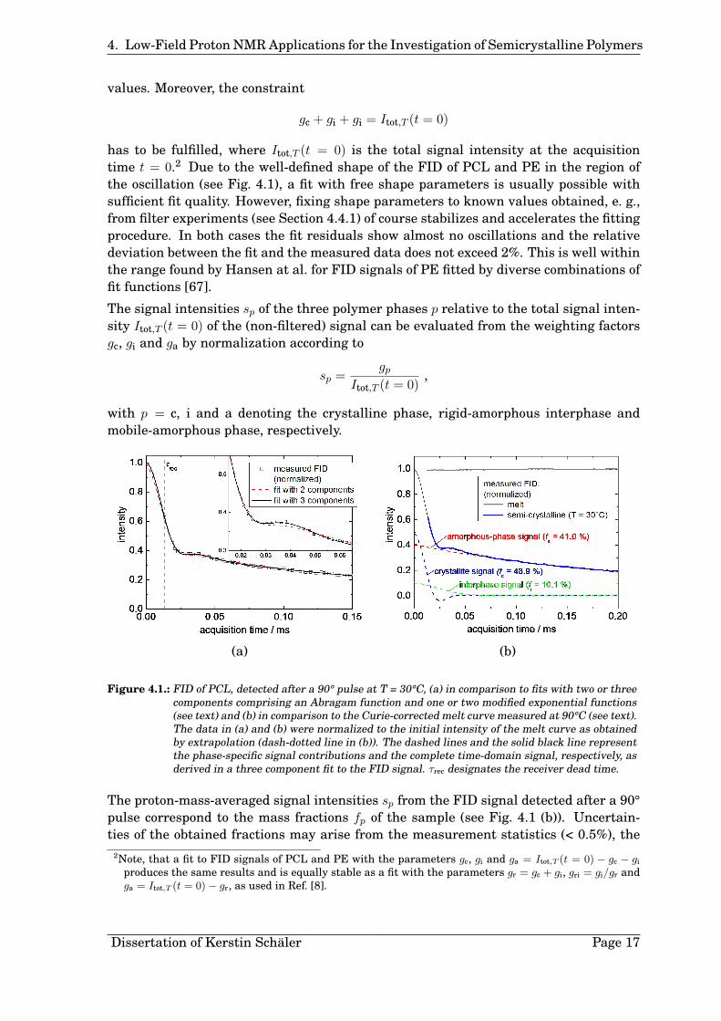
has to be fulfilled, where Itot,T (t = 0) is the total signal intensity at the acquisitiontime t = 0.2 Due to the well-defined shape of the FID of PCL and PE in the region ofthe oscillation (see Fig. 4.1), a fit with free shape parameters is usually possible withsufficient fit quality. However, fixing shape parameters to known values obtained, e. g.,from filter experiments (see Section 4.4.1) of course stabilizes and accelerates the fittingprocedure. In both cases the fit residuals show almost no oscillations and the relativedeviation between the fit and the measured data does not exceed 2%. This is well withinthe range found by Hansen at al. for FID signals of PE fitted by diverse combinations offit functions [67].
The signal intensities sp of the three polymer phases p relative to the total signal inten-sity Itot,T (t = 0) of the (non-filtered) signal can be evaluated from the weighting factorsgc, gi and ga by normalization according to
sp =gp
Itot,T (t = 0),
with p = c, i and a denoting the crystalline phase, rigid-amorphous interphase andmobile-amorphous phase, respectively.
(a) (b)
Figure 4.1.: FID of PCL, detected after a 90° pulse at T = 30°C, (a) in comparison to fits with two or threecomponents comprising an Abragam function and one or two modified exponential functions(see text) and (b) in comparison to the Curie-corrected melt curve measured at 90°C (see text).The data in (a) and (b) were normalized to the initial intensity of the melt curve as obtainedby extrapolation (dash-dotted line in (b)). The dashed lines and the solid black line representthe phase-specific signal contributions and the complete time-domain signal, respectively, asderived in a three component fit to the FID signal. τrec designates the receiver dead time.
The proton-mass-averaged signal intensities sp from the FID signal detected after a 90°pulse correspond to the mass fractions fp of the sample (see Fig. 4.1 (b)). Uncertain-ties of the obtained fractions may arise from the measurement statistics (< 0.5%), the
2Note, that a fit to FID signals of PCL and PE with the parameters gc, gi and ga = Itot,T (t = 0) − gc − gi
produces the same results and is equally stable as a fit with the parameters gr = gc + gi, gri = gi/gr andga = Itot,T (t = 0)− gr, as used in Ref. [8].
Dissertation of Kerstin Schäler Page 17

4. Low-Field Proton NMR Applications for the Investigation of Semicrystalline Polymers
fitting procedure and small temperature deviations during the measurements. Fromthe scatter of the mass fraction data obtained by fits with free shape parameters (seee. g. Fig. 4.2 (b) and Fig. 5.12) we estimate the relative uncertainty of the fractions to besmaller than 5%.
In order to enable a comparison with volume crystallinities obtained, e. g., from SAXSmeasurements, the mass fractions fp can be converted to volume fractions fp,V via
fp,V =
(fp/%H,p
)∑j={c, i, a}
(fj/%H,j
) , (4.7)
taking into account the proton spin densities %H,p of the phases p, calculated by multi-plying the mass density %p of the individual phase by the weight fraction ϕ of protons ina polymer chain molecule (ϕ ≈ 0.088 for PCL):
%H,p = ϕ · %p . (4.8)
Due to the rather similar spin densities of the individual polymer phases, mass andvolume fractions, e. g., of PCL deviate by only 1% to 2% of the absolute quantities, whichis indistinguishable within the uncertainty of the measurement. The mass or volumefraction of the crystalline-phase material is usually referred to as crystallinity.
Each 1H low-field NMR time-domain signal of PCL and PE originating, e. g., from spin-diffusion or Saturation-Recovery experiments can in principle be analyzed in the waydescribed above. However, the receiver dead time τrec of the spectrometer, which is re-quired to ensure the complete decay of the pulse intensity and ranges between 11 µsand 15 µs for the low-field devices used here, prevents a detection of the complete FIDsignal. The initial part of the rapidly decaying signal related to the crystallites is lost,because signal acquisition is not possible during the dead time. Hence, the total inten-sity Itot,T (t = 0) is usually unknown (see Fig. 4.1 (a)). Quantitative data fits are onlypossible, if Itot,T (t = 0) can be estimated based on additional information. For example,in the case of a molten sample, there is no rapid initial signal decay due to the lackof crystallites. Therefore, Itot,Tm(t = 0) at the temperature Tm of the melt is obtainedeasily by an extrapolation of the measured FID data to t = 0 (see Fig. 4.1 (b)). Further-more, to account for changes of the signal intensity due to the different measurementtemperature, a correction can be made here according to Curie’s law [70],
Itot,T1(t = 0) = Itot,T2(t = 0)T2T1
, (4.9)
with T1 and T2 being the temperatures of the two FID measurements. Such a Curiecorrection is necessary in general, to obtain comparable signal intensities from mea-surements at different temperatures. However, equation 4.9 is applicable only if therecycle delay between the individual signal-acquisition scans is long enough to enablecomplete T1 relaxation.
As an example, in Fig. 4.2 (a) the FID signals of PCL at different measurement tem-peratures between the glass transition and the melting point are shown. The curvesare rescaled using Curie’s law (Eq. 4.9). Fits according to the explanations above, usingfree shape parameters, yield the sample fractions given in Fig. 4.2 (b). A significant de-crease in crystallinity and increase in the mobile-amorphous fraction is detected when
Dissertation of Kerstin Schäler Page 18

4. Low-Field Proton NMR Applications for the Investigation of Semicrystalline Polymers
approaching the melting temperature Tf, due to the onset of melting of the less stablecrystallites (pre-melting) [17].
At low temperatures the measured fractions are largely influenced by the glass tran-sition of polymer chains on the NMR time scale. The thermodynamic glass transitionas detected by DSC at cooling rates of about 10 K/s happens to be close to the kineticglass transition measured at frequencies in the range of Hertz, which is based on fluc-tuations inside the sample with typical correlation times on the order of seconds [10].Yet, the NMR glass transition is generated by the freezing of motions with correlationtimes in the range of the inverse dipolar coupling strength, i. e. at about 50 µs. It occursat temperatures Tg,NMR which are 30°C to 60°C higher than the DSC glass transitiontemperature Tg,DSC. When, due to a decrease in temperature, segmental motions in theamorphous phase are slowed down to correlation times higher than some tens of mi-croseconds, i. e. longer than the duration of the measurement, the averaging of dipolarcouplings, being responsible for the slow signal decay, is canceled. In this case, the sig-nal of the (now rigid) chains within the amorphous phase cannot be distinguished frominterphase (or even crystallite) signal anymore. Hence, with decreasing temperaturearound and below Tg,NMR a rising part of amorphous-phase signal is evaluated as inter-phase signal. For this reason the rise of the mobile-amorphous-phase fraction in favor ofthe interphase fraction below Tg,NMR (see Fig. 4.2 (b)) is not a true increase of the massfraction but an artifact arising from the freezing of segmental motions of the polymerchains on the NMR time scale.
(a) (b)
Figure 4.2.: (a) FID signals, detected after a 90° pulse, for PCL at different temperatures between theglass transition and the melting point. The intensities have been corrected according toEq. 4.9 and normalized to Itot,T (t = 0), determined by extrapolation of the melt curve (seetext). τrec denotes the receiver dead time; (b) Signal fractions for PCL, obtained from fitsto the FID signals in (a) with free shape parameters and a reference intensity Itot,T(t = 0)derived from an extrapolation of the melt curve (see text). Above Tg,NMR the signal fractionsrepresent the sample mass fractions fc, fa and fi of crystalline, mobile-amorphous and rigid-amorphous phase, respectively. The solid lines in (b) serve as guides to the eye.
This freezing and unfreezing of chain dynamics is also reflected in the temperaturedependence of the shape parameters T ∗2a and νa of the amorphous-phase time-domainsignal (see Fig. 4.3). Starting at Tg,DSC, at increasing temperatures the onset of theso-called motional narrowing of the NMR spectrum is visible, corresponding to a rise
Dissertation of Kerstin Schäler Page 19

4. Low-Field Proton NMR Applications for the Investigation of Semicrystalline Polymers
of the relaxation time constant T ∗2a due to increasingly averaged dipolar couplings as aresult of growing chain mobility. Moreover, below the NMR glass transition the distri-bution parameter νa of the modified exponential fit function 4.4 takes values below 1(see Fig. 4.3 (b)), indicating a distribution of signals from different micro-environmentswith different relaxation time constants, reflecting the strong dynamic heterogeneity ofthe amorphous regions in the glassy state [73].
Above the NMR glass transition, where all chains within the amorphous regions aremobile, a T ∗2a plateau is reached. Despite a further temperature increase, the chain mo-bility rises only slightly as a result of mobility constraints, such as chain entanglements.Only after the onset of pre-melting a further increase in mobility and T ∗2a is detected (seeFig. 4.3 (a)).
(a) (b)
Figure 4.3.: Shape parameters for the mobile-amorphous phase of PCL as a function of temperature ob-tained from fits to MAPE-filtered FIDs measured at different temperatures. The solid linesare guides to the eye.
In summary, the measurement of 1H low-field NMR FID signals provides the opportu-nity to determine the crystallinity, or more generally the phase fractions, of semicrys-talline polymers and allows the investigation of chain mobility within the amorphousphase to some extent. The measurement relies on mobility differences between theindividual polymer phases and can therefore only yield meaningful phase fractions attemperatures far above the DSC glass transition. The experiment itself requires only ashort measurement time and the data analysis is usually straightforward and can easilybe generalized. However, the fit function has to be adapted for every new sample sys-tem. In the case of PCL and PE an interphase fraction has to be assumed to fit the data.A comparison of crystallinities as obtained from NMR, SAXS and DSC measurementswill be given in Section 6.
4.2. The Magic Sandwich Echo
The Magic Sandwich Echo (MSE) sequence is a so-called time-reversing pulse sequence[80]. It refocuses rapidly decaying NMR signals, which are governed by the action ofstrong multiple dipolar couplings between the nuclear spins of the sample, by reversing
Dissertation of Kerstin Schäler Page 20

4. Low-Field Proton NMR Applications for the Investigation of Semicrystalline Polymers
the dipolar dephasing [81,82].
(a) (b)
Figure 4.4.: Schematic plot of the ’simple’ FID (a) and the Magic Sandwich Echo (MSE) (b) sequence. Allpulses are 90° pulses. The signal loss in the FID caused by the receiver dead-time prob-lem is overcome by using the MSE sequence. The waiting time τ in the MSE sequence iscalculated as τ = (2τp90 + 4τϕ)nMSE, with τp90, τϕ and nMSE being the 90° pulse length, thephase-switching time and the number of MSE cycles, respectively. The duration of the MSEsequence is tseq = 6τ . The MSE phase cycle is ϕ1 = x x x x x x x x, ϕ2 = y y y y x x x x,ϕ3 = x x x x y y y y.
The pulse sequence is depicted in Fig. 4.4 (b). It contains a 90° pulse followed by adelay τ and a so-called sandwich part of duration 4τ , comprising two 90° pulses of thesame pulse phase with two pulse blocks, consisting of 4 90° pulses each, in between.The pulses within each block exhibit the same phase and the phases of the second blockare inverted compared to the ones of the first block.3 After another delay τ the echo isgenerated.
Besides the MSE sequence there is a number of other sequences for the refocusing ofsignal losses due to dipolar dephasing [17, 80, 84]. A main advantage of the sequenceused here is that it serves to bridge the receiver dead time τrec, which causes a signal lossin the FID after a 90° pulse (see Fig. 4.4 (a) and Section 4.1), because the echo appearsonly at a distinct time τ after the last pulse of the sequence. By choosing τ at leastas long as τrec, a virtually dead-time free time-domain signal can be acquired. Besides,a second echo is generated in the middle of the sequence after 3τ which, however, isnot usable, because it appears too soon after the previous pulse. For simplification, inthe following FID’s detected after a single 90° pulse will be termed ’FID’ signals, whileFID’s detected after the application of the MSE pulse sequence will be referred to as’MSE’ signals.
The mode of action of the MSE sequence can be described as a time reversal of theeffects of dipolar couplings on the spin system. It is based on the averaging of dipolarcouplings to zero during the sequence, leaving the system at t = 6τ in a state wheredipolar interactions seemingly have never been present before. This refocusing effectcan be understood by applying Average Hamiltonian theory to the dipolar Hamiltonianof the sandwich part of the pulse sequence (for further explanations see Appendix D.1).
Two adaptations of the sequence have been made compared to the original version.3The inversion of the pulse phases in the second block does not serve to refocus the signal but is necessary
for the compensation of possible phase imperfections [83].
Dissertation of Kerstin Schäler Page 21

4. Low-Field Proton NMR Applications for the Investigation of Semicrystalline Polymers
First, to account for phase-switching times between adjacent pulses which are requiredby the spectrometer, the long burst pulses suggested in Ref. [80] were substituted byblocks of 90° pulses as described above. Moreover, by inverting the phase of the lastpulse compared to the original MSE sequence, in a so-called mixed version we combinedthe MSE with a Hahn echo, in order to refocus signal losses due to magnetic field inho-mogeneities additionally (see Appendix D.1.1) [85,86].
The refocusing action of the MSE sequence relies on the fulfillment of two conditions:
• ωD = const. during the whole sequence and
• ωD � 1/(6τ) [83,86].
Changes of the dipolar coupling strength ωD during the sequence hamper a completeaveraging of the couplings to zero and cause an inefficient signal refocusing and thus asignal loss compared to the FID (see Fig.4.5 (a)). This feature provides the opportunity toinvestigate molecular dynamics on an intermediate time scale, i. e. on the order of tensto hundreds of microseconds, which alter the dipolar couplings during the sequence [83,86–88]. With increasing sequence length the echo amplitude decays with a relaxationtime T2 characterizing the motion (see Section 5.2).
A complete averaging of couplings during the sequence can be achieved only in caseof a short sequence comprising δ pulses. However, pulses of finite lengths with phase-switching times in between as well as pulse imperfections of the pulse phase or thepulse homogeneity cause changes of the mean coupling strength during the differentparts of the sequence, which prevent a complete averaging and result in an increasingsignal loss at rising sequence length tseq [80]. By introducing a small perturbance intothe Average Hamiltonian in a quantum-mechanical calculation, Rhim et al. found thatthe echo attenuation is a result of a too long sequence compared to the inverse couplingstrength (see second condition above) and obeys a t2seq dependence (see Appendix D.1.1)[80]. The signal loss due to strong dipolar couplings is demonstrated in Fig. 4.5 (b)for the case of PCL. The indirect dependence of the refocusing efficiency on the inversecoupling strength can be exploited for filter purposes, i. e. to discard signal from stronglycoupled spins by tuning the sequence length [89,90].
Since, compared to the FID, the decay of the echo intensity as a function of the sequencelength tseq is usually slow and the corresponding spectrum is narrowed appreciably [91],the MSE sequence is furthermore applied for line-narrowing purposes in Magnetic Res-onance Imaging (MRI) [83,85,92].
During the MSE measurements for this work, it turned out that the echo position isslightly shifted to shorter times compared to the expected position marked in Fig. 4.4.This shift increases at rising sequence length, induced by an increase of either thephase-switching time τϕ or the number nMSE of MSE cycles. The latter is demonstratedin Fig. 4.6, presenting a linear dependence of the time difference between measured andexpected echo position on nMSE and the sequence length. Yet, the finite pulse lengthscan be ruled out as a reason for the shift of the echo position, because an elongation andattenuation of the pulses causes a signal attenuation, but no additional time shift of theecho. Presumably, the shift effect results from imperfect pulse phases, and thereforegrows with an increasing number of pulses.
Because a symmetric pulse sequence is favorable for the complete refocusing of signallosses due to off-resonance effects by the hidden Hahn echo within the sequence and for
Dissertation of Kerstin Schäler Page 22
4. Low-Field Proton NMR Applications for the Investigation of Semicrystalline Polymers
(a) (b)
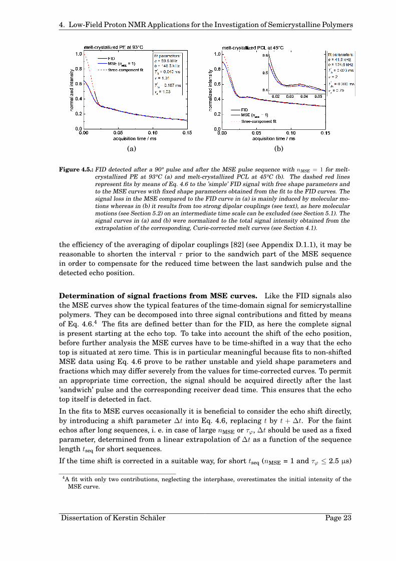
Figure 4.5.: FID detected after a 90° pulse and after the MSE pulse sequence with nMSE = 1 for melt-crystallized PE at 93°C (a) and melt-crystallized PCL at 45°C (b). The dashed red linesrepresent fits by means of Eq. 4.6 to the ’simple’ FID signal with free shape parameters andto the MSE curves with fixed shape parameters obtained from the fit to the FID curves. Thesignal loss in the MSE compared to the FID curve in (a) is mainly induced by molecular mo-tions whereas in (b) it results from too strong dipolar couplings (see text), as here molecularmotions (see Section 5.2) on an intermediate time scale can be excluded (see Section 5.1). Thesignal curves in (a) and (b) were normalized to the total signal intensity obtained from theextrapolation of the corresponding, Curie-corrected melt curves (see Section 4.1).
the efficiency of the averaging of dipolar couplings [82] (see Appendix D.1.1), it may bereasonable to shorten the interval τ prior to the sandwich part of the MSE sequencein order to compensate for the reduced time between the last sandwich pulse and thedetected echo position.
Determination of signal fractions from MSE curves. Like the FID signals alsothe MSE curves show the typical features of the time-domain signal for semicrystallinepolymers. They can be decomposed into three signal contributions and fitted by meansof Eq. 4.6.4 The fits are defined better than for the FID, as here the complete signalis present starting at the echo top. To take into account the shift of the echo position,before further analysis the MSE curves have to be time-shifted in a way that the echotop is situated at zero time. This is in particular meaningful because fits to non-shiftedMSE data using Eq. 4.6 prove to be rather unstable and yield shape parameters andfractions which may differ severely from the values for time-corrected curves. To permitan appropriate time correction, the signal should be acquired directly after the last’sandwich’ pulse and the corresponding receiver dead time. This ensures that the echotop itself is detected in fact.
In the fits to MSE curves occasionally it is beneficial to consider the echo shift directly,by introducing a shift parameter ∆t into Eq. 4.6, replacing t by t + ∆t. For the faintechos after long sequences, i. e. in case of large nMSE or τϕ, ∆t should be used as a fixedparameter, determined from a linear extrapolation of ∆t as a function of the sequencelength tseq for short sequences.
If the time shift is corrected in a suitable way, for short tseq (nMSE = 1 and τϕ ≤ 2.5 µs)
4A fit with only two contributions, neglecting the interphase, overestimates the initial intensity of theMSE curve.
Dissertation of Kerstin Schäler Page 23

4. Low-Field Proton NMR Applications for the Investigation of Semicrystalline Polymers
(a) (b)
Figure 4.6.: (a) Magic Sandwich Echo (MSE) signals for PCL at 40°C detected directly at the end of thereceiver dead time τrec = 11µs for different numbers nMSE of MSE cycles. The straight linesmark the expected, theoretical echo positions. In order to illustrate the deviation betweenexpected and measured echo position, in the inset the measured curves are time-shifted ina way that the expected echo positions appear at t = 0. In (b) the time difference betweenexpected and measured echo position is depicted as a function of the number nMSE of MSEcycles.
the shape of the MSE signal resembles the one of the FID closely for PCL and PE5 (seeFig. 4.5 (b)). This is in agreement with literature results [80,82].
With increasing sequence length (τϕ > 2.5 µs) the shape of the crystallite contribution tothe MSE signal changes compared to the FID (cf. Ref. [80]). However, when ∆t is usedas a variable time-shift parameter in the fits, nevertheless the shape parameters a andb can be kept constant with sufficient quality of the fit.
Also for the shortest possible MSE sequence the measurement curves show a phase-specific signal loss when compared to the FID signal as a result of the phase-specificrefocusing efficiency, which depends on the respective dipolar coupling strength and thepossible occurrence of dynamics on an intermediate time scale. Such effects are knownfor the Solid Echo sequence as well [8,76], where they seem to be even stronger. Like thedipolar coupling strength and motional rates, the signal loss depends on temperature.
In Fig. 4.7 the phase-specific MSE signal loss is depicted for PCL as a function of temper-ature between the glass transition and the melting point in relation to the correspondingmass fractions derived from the FID. For PCL a rather constant portion of MSE crystal-lite signal is lost over the whole temperature range due to strong dipolar interactions.On the other hand the mobile-amorphous phase hardly exhibits any loss at high temper-atures, but a rising deficit at decreasing temperatures around and below the NMR glasstransition, resulting from the slow-down of segmental motions to the intermediate timescale and further, accompanied by rising dipolar coupling strengths. The highest loss isfound for the PCL interphase, supposedly as a result of dynamics on an intermediatetime scale.
To obtain loss-corrected signal fractions, phase-specific correction factors Ccorr,p can bedetermined at every measurement temperature by comparing the signal intensities
5However, insufficient phase cycling can induce distortions of the signal shape, presumably due to pulse-phase imperfections. For a quick check a comparison of the MSE and the FID signal is reasonable. Here,e. g., MSE intensities being larger than in the corresponding FID give hints to an artifact.
Dissertation of Kerstin Schäler Page 24

4. Low-Field Proton NMR Applications for the Investigation of Semicrystalline Polymers
Figure 4.7.: Phase-specific signal loss due to theaction of the MSE sequence (nMSE = 1,τϕ = 2.2µs) in PCL as a function ofthe measurement temperature T , ob-tained by comparison of the normal-ized signal intensities sp from fits tothe MSE curves with the mass frac-tions derived from the correspondingFID signals. The loss values are givenrelative to the sample mass fraction ofthe respective phase. The solid linesserve as guides to the eye.
gMSE,p and gFID,p of each phase p, derived from fits using Eq. 4.6 to the MSE and thecorresponding FID signal, both measured at the same gain:
Ccorr,p =gFID,p
gMSE,p
Once these factors are known for a certain temperature, they can be used to calculatecorrected signal fractions also for filtered MSE experiments (see Section 4.3), performedby using the same experimental parameters as for the ’pure’ MSE measurement.
The MSE sequence can also be applied to determine the mass fractions of a semicrys-talline polymer, if molecular dynamics on the time scale of the sequence length are ab-sent. Here, it is favorable to use the shortest possible sequence6 for the measurement,in order to obtain a signal whose shape and intensity resemble the ones of the FIDclosely. The advantage of using the MSE signal instead of the FID is the better fittingquality and stability in case of the MSE, arising from the fact that there is no missingsignal part due to the receiver dead time (see Fig. 4.4). However, here, the signal frac-tions obtained from the fit have to be converted to mass fractions by correction for MSEsignal loss by means of suitable correction factors (see above). These again have to bedetermined by means of the corresponding FID. The mass fractions obtained from fitsto the MSE signal deviate from the FID results by up to 2% on an absolute scale. Thisis usually within the uncertainty limits.
In summary, the Magic Sandwich Echo sequence serves to overcome the receiver deadtime problem of the FID measurement and can be applied to measure sample massfractions in semicrystalline polymers (see Chapter 8) although corrections of the phase-specific intensity loss due to the MSE sequence are necessary. Yet, the possible appli-cations of the MSE sequence exceed the generation of a virtually dead-time free FID byfar. Rather, the MSE sequence can be used as a dipolar mobile-phase filter and allowsthe investigation of molecular dynamics on an intermediate time scale (see Section 5.2).
6The shortest possible sequence is the one where nMSE = 1 and τϕ is as small as possible without violatingthe condition τ = (2τp90 + 4τϕ) ≥ τrec (cf. Fig. 4.4 (b)).
Dissertation of Kerstin Schäler Page 25
4. Low-Field Proton NMR Applications for the Investigation of Semicrystalline Polymers
4.3. Proton Spin Diffusion in Semicrystalline Polymers
The process of 1H spin diffusion has been known for many years and is frequently ex-ploited in order to explore microdomain structures and sizes in heterogeneous poly-mer systems [77, 78, 93–105]. Existing work on NMR spin-diffusion measurements ispredominantly concerned with block copolymers [94–96, 104, 106–112], periodic copoly-mers [113, 114] and semicrystalline polymers [77, 95, 97, 115–119]. However, the ex-periments are not bound to longe-range order or periodic structures. Investigations,e. g., in purely amorphous polymers [102, 120] and blends of them are possible as well[100, 105, 121–125]. Up to now, moreover, there is a number of studies on more ’ex-otic’ materials, such as core-shell latex particles [126–129] and water layers aroundthem [130], polymeric proton exchange membranes [99], hybrid siloxane networks [131],amphiphilic co-networks [132] and membrane proteins [133,134]. Glassy layers in filledelastomers represent a further potential field of application.
Apart from being non-destructive one main advantage of the method is that it does notnecessitate sample modification before measurement, such as staining, deuteration orany other kind of contrast enhancement, as it exploits pre-existing differences in NMRinteraction strengths. Length scales of a few up to a few hundred nanometers are acces-sible by spin-diffusion NMR, as comparable to SAXS measurements [17]. Furthermorespin-diffusion measurements provide information about interphases, which are difficultto obtain by other techniques [103,111,126,127], and using appropriate filter sequencesthey also serve to gain information about interactions of neighboring proton spins viathe investigation of spin dynamics [135].
In semicrystalline polymers spin-diffusion experiments enable the determination of lam-ellar thicknesses, provided that spin-diffusion coefficients are known. Vice versa, withknown domain sizes spin-diffusion coefficients can be obtained. Additionally, informa-tion can be gained about the dimensionality of the spin-diffusion process [101] and henceabout details of the polymer-phase morphology.
Macroscopic magnetization relies on the magnetic dipole moments of the nuclei in asample and is coupled to their spin states. The term spin diffusion denotes the transferof magnetization between neighboring spins mediated by dipolar couplings [17]. Thistransfer is not a true diffusion process involving material transport7 but it is based on aquantum-mechanical exchange process which, in a simplified picture, can be visualizedas reversible spin flip-flop processes. It occurs, if magnetization is distributed nonuni-formly over a sample with the result that these differences will be compensated aftera certain time. The effect was named by Bloembergen in 1949, who found drasticallyaccelerated T1 relaxation in anorganic crystal compounds in the presence of paramag-netic impurities with relaxation times deviating from the theoretical value by a factorof 106 [136]. He discovered a magnetization transfer (i. e. spin diffusion) from the sur-roundings of the rapidly relaxing paramagnetic centers to the more slowly relaxing bulkmaterial to be the reason for this behavior.
Based on a quantum-mechanical calculation (see Appendix F.1) it can easily be demon-strated for a system of isolated pairs of spins 1/2, that a magnetization transfer in facttakes place under dipolar interaction [17]. The transfer is efficient only if the dipolar
7However, the designation spin diffusion is well-established because at appropriate length scales themagnetization transfer can be described by Fick’s second law for diffusion [17,116,136,137].
Dissertation of Kerstin Schäler Page 26

4. Low-Field Proton NMR Applications for the Investigation of Semicrystalline Polymers
coupling strength is larger than the difference between the resonance frequencies of thenuclei involved. In essence, in the NMR spectrum there must be an adequate overlapof the spectral lines of these coupling nuclei [17]. In polymers the density of protons ishigh and their distances are small, e. g. ∼0.18 nm between the two protons of a CH2
group, usually resulting in an efficient proton spin-diffusion process due to strong dipo-lar couplings (∼20 kHz) compared to the chemical shift frequency difference amounting,e. g., to up to 4 kHz for a 400 MHz spectrometer (δ ∼ 1 ppm to 10 ppm). By contrast,owing two their small natural abundance of 1.1 %, distances between the NMR-active13C nuclei in polymers are typically larger (∼0.8 nm) and accordingly the resulting dipo-lar couplings are considerably weaker (∼15 Hz) than for protons and low compared totypical chemical shift frequency differences (in the range of kilohertz), so that directspin diffusion between these nuclei is very inefficient. It proceeds slowly, i. e. with timeconstants of tens of seconds, and can usually be neglected [17,138]. Nevertheless thereare techniques which allow for the detection of 13C spin diffusion [17].
Contrary to material diffusion, spin diffusion is a coherent process, which can be re-versed by inversion of the dipolar interaction. The Magic Sandwich Echo (MSE) se-quence is an example for a sequence accomplishing a time reversal (see Section 4.2).
4.3.1. The Spin-Diffusion Experiment
(a)
(b)
Figure 4.8.: Basic scheme of a 1H NMR low-field spin-diffusion experiment:(a) generalized pulse sequence,(b) development of the magne-tization profile in a two-domainsample system during the ex-periment [17, 139]; the bottomrow depicts the free inductiondecay (FID) of the transversemagnetization measured at thecorresponding points in time,exemplarily for the case of amobile-phase-selected low-fieldexperiment.
Spin-diffusion experiments in heterogeneous polymer systems allow the observation ofmagnetization transfer from source to sink domains. For this pupose magnetizationin one of the polymer phases (denoted as source) is selected while it is depleted in therest of the system (referred to as sink) by means of specific filter sequences (see Sec-tion 4.4). Thus, spatial gradients of magnetization are generated between source andsink domains within the sample, which induce a magnetization transfer (i. e. spin dif-fusion) during the subsequent mixing time τdiff towards the initially non-polarized sinkphase, until at long τdiff the magnetization is evenly distributed again (see Fig. 4.8).The redistribution of magnetization among the polymer phases can directly be observedin the corresponding signal intensity, provided that phase-selective signal detection ispossible. This is the case only if the polymer phases exhibit differences in NMR interac-tions, such as chemical shift, dipolar coupling strength, relaxation times and so on. Inthis case the equilibrium intensities of the NMR signals provide information about the
Dissertation of Kerstin Schäler Page 27

4. Low-Field Proton NMR Applications for the Investigation of Semicrystalline Polymers
phase composition of the sample.
In the course of the spin-diffusion process the magnetization first reaches structuresclose to the magnetization source. Therefore information about the local arrangementof the polymer phases can be deduced. Furthermore the speed of the re-equilibrationdepends on the domain sizes and dipolar coupling strengths within the phases. The uni-form magnetization distribution is, e. g., reached rapidly for small domains and strongcouplings. Thus, the development of magnetization with increasing mixing time τdiffyields information on domain sizes (and geometry) and on characteristic spin-diffusioncoefficients of the phases (see Chapter 7).
The selection of magnetization as the first step of a spin-diffusion experiment is ac-complished by a filter sequence (see Section 4.4) on the basis of differences in NMRinteraction strengths of the individual polymer phases in the sample. However, becauseof a lack in chemical shift resolution, in low-field measurements one usually exploitsdifferences in local chain mobility and dipolar coupling strength between the phases forfiltering the magnetization as well as for phase-specific detection. Hence, only systemswith dynamic heterogeneity on an appropriate length scale are suited for this purpose.
4.3.2. The Differential Equation for Spin Diffusion
Experimental proton spin-diffusion data can be analyzed based on a solution of the dif-ferential equation describing the spin-diffusion process. This equation is easily derivedunder the assumption of a linear arrangement of spins in a row [17]. In this case the de-velopment of magnetization Mi in direction of the magnetic field at the site i of one spin,exchanging magnetization with its neighboring spins at i − 1 and i + 1 with a constantrate R during a time ∆t via dipolar couplings, can be described by a Master equation:
∆Mi
∆t= (RMi+1 −RMi) + (RMi−1 −RMi) .
Reformulating this equation yields
∆Mi
∆t= D
(Mi+1 −Mi)− (Mi −Mi−1)
(∆x)2, (4.10)
with ∆x andD = R(∆x)2 being the distance between the spins in the row and the (in thiscase constant) spin-diffusion coefficient, respectively. For 1H spin diffusion in polymers,because of the high proton density, it is allowed to transform this discrete equationinto a continuous one, i. e. to approach ∆t → 0 and ∆x → 0. In this limit one finds acontinuous differential equation, Fick’s second law for one-dimensional magnetizationtransport, with the spatial coordinate x, the time coordinate t and a constant diffusioncoefficient D:
∂M(x, t)
∂t= D
∂2M(x, t)
∂x2. (4.11)
The general equation for a k-dimensional process and a variable diffusion coefficient Dreads:
∂M(r, t)
∂t= ∇ (D(r, t)∇M(r, t)) =
1
rk−1∂
∂r
(rk−1D
∂M(r, t)
∂r
). (4.12)
Here, r is the spatial coordinate and k the number of orthogonal dimensions along which
Dissertation of Kerstin Schäler Page 28

4. Low-Field Proton NMR Applications for the Investigation of Semicrystalline Polymers
a gradient of magnetization exists [102]. Depending on the diffusion scenario the dimen-sion parameter k can adopt the following values [139]:
k =
1 for a lamellar system,2 for cylinders in a matrix and3 for spheres or cubes in a matrix.
In case of a constant diffusion coefficient D and a lamellar arrangement of domainsEq. 4.12 reduces to Eq. 4.11.
If there are further reasons for changes in magnetization apart from spin diffusion,for instance due to additional magnetization sources or sinks or material transport,corresponding terms have to be incorporated into the diffusion equation. True chaindiffusion through the crystallites takes place, e. g., in PE or poly(ethylene oxide) [140].If spin and chain diffusion occur on a similar time scale, a second diffusion term has tobe supplemented to Eq. 4.12. However, this is not necessary for crystal-fixed polymers.Effects of longitudinal relaxation are introduced by means of an additional term 1
T1(M0−
M(r, t)) [141, 142] (cf. Section 7.3), where M0 denotes the equilibrium magnetization atlong times t→∞ und T1 is the longitudinal relaxation time constant.
The spin-diffusion equation 4.12 was solved analytically by many authors for special ge-ometries similar to the situation in heterogeneous polymer systems, i. e. arrangementsof two or three polymer phases and distinct dimensionality k of the spin-diffusion pro-cess, considering different initial and boundary conditions [89,95,97,101,102,116,139,142–144]. Solutions for k > 1 can be derived by k-fold multiplication of the solution fork = 1, if the diffusion process is assumed to be uniform in each of the dimensions [139].A one-dimensional geometry corresponds, e. g., to the idea of the idealized lamellar ar-rangement of crystallites in a semicrystalline polymer and will be used for data analysisin Chapter 7.
Regrettably, analytical solutions of Eq. 4.12 are complex and difficult to handle. Further-more, they cannot be obtained under consideration of T1 relaxation for the geometriesnamed above. This does not pose a problem for the analysis of spin-diffusion data, ifeither spin diffusion or T1 relaxation clearly dominates the time development of magne-tization. The former applies for very slow T1 relaxation compared to the characteristicspin-diffusion time (d2/D) [141, 145], i. e. T1 >> (d2/D), the latter in the opposite caseT1 << (d2/D). Here, (d2/D) is the time needed to transfer magnetization through a re-gion of thickness d assuming a constant diffusion coefficientD. However, once spin diffu-sion and T1 relaxation take place on the same time scale, (d2/D) ≈ T1, the relaxation hasto be taken into account in the analysis, as it influences the development of longitudi-nal magnetization during the mixing time.8 In semicrystalline polymers typical domainsizes d amount to ∼10 nm and spin-diffusion coefficients range between 0.1 nm2/msand 1 nm2/ms, resulting in characteristic diffusion times (d2/D) between 100 ms and1000 ms. In strong magnetic fields longitudinal relaxation usually proceeds slowly, withtypical proton T1 values at 400 MHz being in the range of seconds. Hence, the magneti-zation development is dominated by spin diffusion. Yet, at low field strengths T1 is muchsmaller, ranging between ∼ 50 ms and several hundreds of milliseconds for a 20 MHz
8On the other hand, in a Saturation-Recovery experiment for the determination of T1, spin diffusionoccuring during the waiting period τsatr has to be considered (see Section 5.1).
Dissertation of Kerstin Schäler Page 29

4. Low-Field Proton NMR Applications for the Investigation of Semicrystalline Polymers
Figure 4.9.: Magnetization development in a simulated spin-diffusion experiment for a one-dimensionalthree-phase system, i. e. a periodic sequential arrangement of source and sink domains withinterphases between them, under the influence of T1 relaxation for different settings of T1.Without the effect of T1 relaxation, the intensity ratio at long mixing times τdiff represents themass fractions of the distinct phases in the system. The simulation parameters are given inthe table. The simulation is adapted to an experimental setup where longitudinal relaxationcauses an intensity decay due to alternating storage of magnetization along and opposite tothe direction of the magnetic field in subsequent scans.
spectrometer. Here, T1 is in the order of the characteristic spin-diffusion time and T1relaxation cannot be neglected. Fig. 4.9 shows the effect of T1 relaxation on the mag-netization development in a spin-diffusion experiment simulated for a one-dimensionalspin-diffusion scenario.
There are methods for reducing the T1 influence in spin-diffusion experiments. One op-tion is the alternating storage of magnetization along and opposite to the direction ofthe magnetic field by a so-called z filter after the selection period in subsequent scans,to partially eliminate relaxation effects from consecutive measurements [17]. This tech-nique works properly only if the magnetization is destroyed after the selection period.Yet, this is not possible in a spin-diffusion experiment, as in this case no magnetizationtransfer could take place anymore [146]. For magnetization unequal to zero this proce-dure induces a decay of magnetization (see Fig. 4.9), which can be analyzed more conve-niently than a build-up resulting from measurements without z filter. It was thereforeused in all spin-diffusion measurements discussed in the following. As an alternative a180° pulse can be inserted during the mixing time τdiff in a way that T1 effects before andafter the pulse cancel each other out. However, this method operates effectively only incase of a single relaxation time of the whole system [146]. As the different componentsof a heterogeneous polymer system usually differ in their T1 time constants, there isno other option up to now than to solve the differential equation 4.12 numerically afterintroduction of a T1 relaxation term [8,108,109,141,147] (see Section 7.3).
4.4. NMR Filter Sequences
A variety of filter sequences usable for low-field spin-diffusion experiments can be foundin literature. So-called T2 filters relying on different T2 relaxation times of the polymercomponents serve to select magnetization in mobile polymer phases. Well-known ex-
Dissertation of Kerstin Schäler Page 30

4. Low-Field Proton NMR Applications for the Investigation of Semicrystalline Polymers
amples of this type are the Hahn echo filter [96, 133, 134, 148] and the Goldman-Shenfilter [76,113,116,117,131,147,149–151]. Yet, the latter creates signal disturbances, theorigin of which still seems to be under discussion [8,117,150].9 Dipolar filters base uponthe differences in dipolar coupling strengths between the polymer phases. A part of thisfilter class including, e. g., the 12-pulse sequence [94,98,106–108,112,120,127,132,153],the Magic Sandwich Echo (MSE) [89,95,110,144] and the Magic And Polarization Echo(MAPE) [8] exploits the incomplete averaging of the dipolar couplings in case of longsequence durations in terms of long cycle times in the Average Hamiltonian sense (seeAppendix D.1.1) to achieve a filter action. They allow for the selection of magnetiza-tion in mobile polymer components. For selecting rigid-phase magnetization double-quantum filters can be employed [78,97,101,103,144], as originally proposed by Graf etal. [154] for 2D measurements in combination with sample spinning and refined by Baand Ripmeester [155] for usage in static 1D experiments.
(a) (b)
Figure 4.10.: Schematic sketch of the MAPE dipolar filter sequence (a) and the double-quantum filtersequence (b). Both include a z filter for usage in spin-diffusion experiments (see Section 4.3).The narrow bars in the plots denote 90° pulse and the broad ones in (b) represent 180°pulses. The two ’sandwich’ pulse blocks of length 2τM in the MAPE sequence in (a) arecomposed of four 90° pulses each, separated by intervals (2)τϕ as in the case of the MSEsequence (see Figs. 4.4 and D.2). The duration of the MAPE filter amounts to 6τM withτM = 2τp90 + 4τϕ. The MAPE phase cycle is ϕ1 = y y , ϕ2 = y y and ϕ3 = x x and the DQphase cycle is ϕDQ = y x y x.
For the investigations presented in this thesis, two filter sequences were used, whichproved to work well in blockcopolymers [8,156]:
• the MAPE sequence and
• a double-quantum filter.
Both sequences are depicted schematically in Fig. 4.10. Their adaptation to an appli-cation to semicrystalline polymers is demonstrated for the case of PCL in the followingsubsections. As an example, Fig. 4.11 shows the filtered time-domain signals in compar-ison to the FID and MSE signal for PCL.
9The utilization of T1 filters in spin-diffusion experiments is unfavorable. In case the difference of theapparent T1 relaxation times between the polymer components is high enough to be appropriate forfiltering, spin diffusion must be very slow, as otherwise it would soon have equilibrated the magnetiza-tion discrepancy due to this T1 difference in a T1 measurement and only a small apparent T1 gap wouldhave resulted. Such a slow spin-diffusion process, however, can only transfer magnetization over veryshort distances precluding a meaningful analysis of the diffusion data [17]. Moreover, T1,% filters, e. g.,the Packer sequence for selecting rigid-phase magnetization [141], cause problems inasmuch as spindiffusion already occurs during the filtering process. Thus, the beginning of the spin-diffusion processis not accessible for detection and therefore small domain sizes cannot be measured [17,152].
Dissertation of Kerstin Schäler Page 31

4. Low-Field Proton NMR Applications for the Investigation of Semicrystalline Polymers
Figure 4.11.: Comparison of a FID and MSE sig-nal for PCL at 45°C with signals fromspin-diffusion experiments for a veryshort mixing time τdiff = 0.21 ms,using a MAPE (τϕ = 37 µs) and adouble-quantum filter (τDQ = 13.8 µs)as depicted in Fig. 4.10. All signalswere normalized with respect to thetotal FID intensity at t = 0, de-rived from a Curie-corrected FID ofthe molten sample.
4.4.1. The MAPE Dipolar Filter Sequence
Similar to the MSE sequence the MAPE sequence comprises a ‘sandwich‘ part consist-ing of blocks of 90° pulses between two flanking pulses (see Fig. 4.10 (a)). Moreover, asfor the MSE, the mode of action is based on the refocusing of rapidly decaying signal dueto strong dipolar interactions (see Appendix D.1.2). In contrast to the MSE sequence,here the ‘sandwich‘ pulses are directly applied to longitudinal magnetization (polariza-tion) instead of tranverse magnetization. The generated echo is therefore named Magicand Polarization Echo (MAPE) [8]. As the MAPE refocusing efficiency is reduced incase of too strong dipolar couplings (cf. Section 4.2), the MAPE sequence, like the MSEsequence, can be used as a dipolar filter. Omitting the unnecessary generation of trans-verse magnetization, it is even more direct than the MSE filter.
The MAPE dipolar filter serves to select magnetization in the slowly relaxing mobile-amorphous phase of a semicrystalline polymer due to weak dipolar couplings there. Forthis purpose the filter length 6τM has to be set in a way, that the refocusing condition6τM � 1/ωD (see Section 4.2) is violated for the rather strongly coupled crystalline andinterphase regions, but fulfilled for the weakly coupled mobile-amorphous phase, sothat the crystalline-phase and interphase signal is filtered out from the total signal anddiscarded. The parameter for tuning the filter action is the inter-pulse spacing τϕ.
In Fig. 4.12 (a) MAPE-filtered time-domain signals, detected after application of theMSE sequence, are depicted to demonstrate the effect of the filter length variation. Incase of PCL it is not possible to choose a perfect filter duration because a clear criterionto distinguish between the interphase and the mobile-amorphous-phase signal cannotbe discerned. The curve shapes are rather unspecific except for the shortest durations.Fitting the data with a modified (stretched or compressed) exponential I0 exp(−t/T ∗2 )ν ,starting with the curves for the longest filter, reveals a continuous change in curve shapeas indicated by a continuous decay of T ∗2 and ν (see Fig. 4.12 (b)). This finding hints ata gradient of mobility through the rigid-amorphous and mobile-amorphous phase. Suchgradients have been found before, e. g., in investigations on segmented poly(urethanes)using a Goldman-Shen filter [151]. When fitting the MAPE-filtered data with a sum ofthree modified exponentials, starting with the curve for the shortest filter, one of thethree fit contributions disappears at an inter-pulse spacing τϕ between 14 µs and 18 µs,and a second one between 36 µs and 38 µs. These vanishing components are interpretedas crystallite and interphase signal component, respectively. Hence, for PCL one MAPE
Dissertation of Kerstin Schäler Page 32

4. Low-Field Proton NMR Applications for the Investigation of Semicrystalline Polymers
(a) (b)
Figure 4.12.: (a) MAPE-filtered MSE curves for PCL at 45°C, detected in spin-diffusion experiments witha short mixing time τdiff = 10 µs and different inter-pulse delays τϕ in the MAPE ’sandwich’blocks. The inset shows the curve chosen as the amorphous-phase signal with a correspond-ing fit using a modified (stretched or compressed) exponential function; (b) Parameters T ∗2and ν from a fit with a single modified exponential function to the data depicted in (a) as afunction of the MAPE inter-pulse delay τϕ (see text).
cycle with an inter-pulse delay τϕ = 37 µs was used throughout the measurements toisolate the signal of the mobile-amorphous phase.
Mobile-phase-filtered signals are easily detected by using the spin-diffusion sequencedepicted in Fig. 4.8 with the MAPE filter and a very short mixing time to avoid spindiffusion. From these signals the shape parameters T ∗2a and νa can be determined sep-arately by a fit with a modified exponential function as described in Section 4.1 andused as fixed parameters in fits to FID or MSE signals to stabilize and accelerate the fit.But, as the choice of the MAPE filter length affects the shape of the signal ascribed tothe mobile-amorphous phase, it slightly influences the mobile-amorphous fraction, mea-sured in the sample, as well as the shape parameters of the interphase signal and thedetected interphase fraction, obtained from a fit to the FID or MSE. The effect cannot beavoided and represents a source of uncertainty in the determination of the phase frac-tions. It should, in particular, be considered when comparing data sets detected withdifferent MAPE filter lengths. For PCL, an elongation of the MAPE inter-pulse delay byabout 8 µs (from τϕ = 38 µs to 46 µs) results in a decrease of the fraction of the mobile-amorphous phase and an increase of the fraction of the rigid-amorphous interphase byup to 2 % each, while the sum of both fraction stays constant. A shortening of the filterlength, however, causes stronger deviations.
4.4.2. The Double-Quantum Filter Sequence
Strong dipolar couplings between spins create a complex network of interacting spins inwhich multi-quantum coherences, involving orientation correlations between interact-ing spins (see Appendix C) [53], can be excited by certain rf-pulse sequences [54, 155].For the investigations presented herein, a well-known and simple pulse sequence forexcitation of multi-quantum coherences was used as a double-quantum filter for theselection of magnetization in the rigid polymer phase (see Fig. 4.10 (b)) [154,155,157].
Dissertation of Kerstin Schäler Page 33

4. Low-Field Proton NMR Applications for the Investigation of Semicrystalline Polymers
The mode of action of the sequence is demonstrated for a system of isolated pairs of spins1/2 in the Appendix D.2 and shall be described here only briefly. The sequence is devidedinto a preparation and a reconversion part. The former, comprising two 90° pulses,separated by a short time interval τDQ, accomplishes the field-independent excitationof double-quantum coherences in the sample.10 As such a coherence itself cannot bedetected directly, it is reconverted into longitudinal magnetization in the second halfof the sequence by repeating the first half, however, applying a 4-step phase cycle overthe pulse pair (see Appendix D.2). Signal detection is achieved here by means of theMSE sequence for refocusing rapidly decaying crystallite signal. (In practice this isagain realized by using the spin-diffusion sequence depicted in Fig. 4.8 with a very shortmixing time.) The 180° pulses in the middle of the excitation and reconversion partseliminate effects due to resonance offsets and magnetic field inhomogeneity during thecorresponding period in the sequence [157,158].
The efficiency of the excitation and reconversion of double-quantum (DQ) coherences,i. e. the portion of originally longitudinal magnetization which is converted into DQcoherence and reconverted back into magnetization, depends on the product of thestrength of the dipolar interactions between the spins and the duration of the excitationtime τDQ [54]. The longer the excitation time (within a certain range) or the strongerthe couplings, the more magnetization is converted, and the higher is the final signalintensity.11 Using a short, fixed excitation time τDQ, the sequence excites DQ coherencesefficiently only in strongly coupled sample regions, such as the crystallites in semicrys-talline polymers. Hence, the measured signal intensity originates from these regionsonly. This filter effect shall be used here to select crystallite magnetization. As the T1relaxation does not affect DQ coherences, it does not influence the filtered signal alsofor long filter durations [155]. This feature makes the filter suited for spin-diffusionexperiments. However, there is a strong signal loss due to the filter, as only a portion ofthe crystallite signal is converted into DQ coherence and back.
Figure 4.13.: Double-quantum-filtered MSE sig-nals for PCL at 30°C, detected inspin-diffusion experiments with ashort mixing time τdiff = 20 µs, forvarying excitation times τDQ. The in-set shows the total signal intensitiesat t = 0 as a function of τDQ.
By changing the excitation duration τDQ the filter action can be tuned. In the ideal case,only magnetization from spins in crystalline regions should be selected. In Fig. 4.13 DQ-filtered MSE signals of PCL are depicted for different excitation times. As expected, with
10Additionally, the sequence also excites higher order coherences, but only to a negligible extent at theshort excitation times τDQ used here [40].
11This provides the opportunity to derive the dipolar coupling strength, e. g., in polymer networks, bymeasuring the reconverted double-quantum intensity as a function of τDQ [40].
Dissertation of Kerstin Schäler Page 34

4. Low-Field Proton NMR Applications for the Investigation of Semicrystalline Polymers
increasing τDQ magnetization from more weakly coupled spins in the interphase andthe mobile-amorphous phase is increasingly selected, indicated by the rising portion ofslowly decaying signal. The total signal intensity is built up until a maximum is reachedat τDQ,max ≈ 16 µs. It decays again at higher τDQ due to molecular motions which changethe dipolar coupling strength on the time scale of the sequence length and thus hamperan efficient reconversion of DQ coherences [40].
At every excitation time τDQ the filtered PCL signal contains a slowly decaying mobile-phase-like component (see Fig. 4.13) which even does not vanish near the DSC glasstransition (where it still originates 4% of the total signal intensity at τDQ = 13 µs). Sucha deficit in DQ filter efficiency is known from literature (cf. Ref. [95]) and is present alsofor a poly(styrene)-poly(butadiene) diblock copolymer (see Fig. 4.15). Actually, fittingthe DQ-filtered MSE signals of PCL with an appropriate quality is possible only us-ing a three-component function as given by Eq. 4.6, while a two-component function isless suited to describe the data (see Fig. 4.14 (a)). Accordingly, the frequency spectrum,i. e. the Fourier transform of the filtered MSE signal, shows a superposition of a broadline related to the crystallites and two smaller, more narrow components, which seem-ingly correspond to interphase and mobile-amorphous phase (see Fig. 4.14 (b)). More-over, at very short mixing times τdiff < 0.1 ms the signal component associated with themobile-amorphous phase is enlarged compared to longer mixing times τdiff ≈ 0.21 ms.This is probably a filter artifact, the reason of which remains unclear. The diffusion ofmagnetization from crystallites to the interphase sets in already at τdiff ≈ 0.5 ms, andproceeds to parts of the mobile-amorphous phase during the first 3 ms. This should beconsidered when selecting the settings for the measurement of crystalline-phase-filteredsignals.
(a) (b)
Figure 4.14.: (a) Double-quantum-filtered MSE signal for PCL at 45°C, detected in a spin-diffusion ex-periments with a short mixing time τdiff for an excitation time τDQ = 16 µs compared to fitsusing two and three components (see text); (b) normalized Fourier transform of the signal in(a) with Fourier transformed fit components from the three-component fit, marked c, i anda, denoting crystalline-phase, interphase and mobile-amorphous-phase signal, respectively.
Powder Averaging. For glassy samples it is known that the magnetization left bythe DQ filter is inhomogeneous in its strength throughout the material, because, accord-ing to the orientation of the interconnection vectors of dipolarly coupling spins (cf. Sec-
Dissertation of Kerstin Schäler Page 35

4. Low-Field Proton NMR Applications for the Investigation of Semicrystalline Polymers
tion 3.3), different chain segments exhibit different coupling strengths. At short exci-tation times τDQ < τDQ,max, longitudinal magnetization arising from the most stronglycoupled spins is selected. It originates from dense sample regions with spin interconnec-tion vectors being oriented preferably in the direction of the magnetic field. In absenceof further rf pulses this magnetization is now redistributed within the sample, due to 1Hspin diffusion, reaching also more weakly coupled parts of the glass with unfavorablespin pair orientation. After a suitably long mixing time τdiff a re-equilibration of themagnetization is accomplished (cf. [158]). This equilibrating process is called powderaveraging and is accompanied by a decrease in the average dipolar coupling strength ofthe polarized material to an equilibrium value, reached for the uniformly magnetizedglass.
The powder averaging is demonstrated in Fig. 4.15 for a poly(styrene)-poly(butadiene)(PS-PB) block copolymer at 45°C with a glassy PS phase and a rubbery phase containingmainly PB [159]. Here, the DQ filter was used to select magnetization from the glassyPS phase. The decrease in the measured, mean coupling strength during the equilibra-tion is reflected by the slow-down of the decay of the DQ-filtered MSE signal and thedecrease in the second moment M2 of the line shape with increasing mixing time τdiff,approaching the equilibrium value derived from an unfiltered MSE signal.
Figure 4.15.: Double-quantum-filtered MSE signals for a PS PB block copolymer at 45°C (upper left) andPCL at 30°C (upper right), detected in spin-diffusion experiments for a short excitationtimes τDQ at varying mixing time τdiff as indicated in the plots, and second moment M2 ofthe line shape for the same samples and temperatures (lower row; left: PS PB, right: PCL)as a function of the mixing time τdiff for various excitation times τDQ. The intensity in theupper-row graphs, obtained as spectrometer output data, is given in arbitrary units.
At long excitation times τDQ > τDQ,max the filter selects magnetization from rather
Dissertation of Kerstin Schäler Page 36

4. Low-Field Proton NMR Applications for the Investigation of Semicrystalline Polymers
weakly coupled regions within the glassy phase (and interphase), while it depletes mag-netization from the strongly coupled glassy regions. This occurs in analogy to the filteraction of the MAPE (and MSE) filter at long filter durations
(� ω−1D
), due to imper-
fections of the sequence which cause an insufficient time averaging of the spin inter-actions12 [155] inducing a loss of signal from strongly coupled regions.13 Here, the re-equilibration is accomplished by a magnetization transfer from more weakly to morestrongly coupled spins within the glassy domains, leading to an increase of the aver-age coupling strength of the polarized material and the second moment M2 with risingmixing time (see Fig. 4.15).
However, the situation is different in semicrystalline polymers, such as PCL. As demon-strated in the right column of Fig. 4.15, indeed M2 of the crystallites, determined fromDQ-filtered MSE signals, decreases with rising excitation time, as a result of the de-creasing average coupling strength of the material excited by the filter (see above). Atlarge excitation times τDQ > τDQ,max also values below the equilibrium value for uni-formly magnetized crystallites (derived from a non-filtered MSE signal) are reached.However, no equilibration due to a redistribution of magnetization can be seen at risingmixing time. Instead, the second moment M2 of the line shape and hence the dipolarcoupling strength remains constant.
These findings can be explained by considering the phase morphology in PCL. In thecrystalline lamellae with their (more or less) all-trans chain conformation, the spin-spininterconnection vectors of the two protons bonded to a carbon atom all have the samedirection with respect to the magnetic field (see Fig. 4.16) and hence exhibit the samecoupling strength.14 Moreover, within their stacks the lamellae are arranged parallely.Thus, after application of the DQ filter magnetization should be distributed uniformlywithin the crystalline material of a stack of lamellae according to the distinct orien-tation of the spin pairs and the corresponding coupling strength. Yet, as in a powdersample the stacks are isotropic in their orientational distribution (see Fig. 4.17), differ-ent stacks possess different magnetization levels. The measurement results depictedin Fig. 4.15 indicate that missing magnetization in one stack cannot be compensatedby spin diffusion from other stacks with a higher magnetization level at short mixingtimes. The lack in magnetization transfer is presumably caused by a missing directcontact between the lamellae of different stacks, which forces magnetization to passthe amorphous regions first. However, the latter process is slow because of the smalldiffusion coefficient of the mobile-amorphous phase (see Section 7.1). By contrast, theglassy PS regions in the block copolymer contain chains with different segmental orien-tations and thus varying dipolar coupling strengths throughout the individual domains,enabling the equilibration at short mixing times.
Because of the missing equilibration of the magnetization distribution within the crys-talline phase of PCL, for filtering purposes an excitation time τDQ should be used, whichdirectly generates the most uniform magnetization distribution in all crystallites. Onecan easily find an excitation time, where M2 of the filtered signal agrees well with the
12In the case of too long sequences (or too strong couplings, respectively) higher order effects in the AverageHamiltonian become too large to be neglected (see Appendix D.1)
13Hence, the DQ filter is in principle also suitable as a mobile-phase filter, when an appropriately longexcitation time is used (cf. Ref. [95]).
14The mean dipolar coupling strength is dominated by the coupling between those geminal protons as aresult of their close proximity.
Dissertation of Kerstin Schäler Page 37

4. Low-Field Proton NMR Applications for the Investigation of Semicrystalline Polymers
Figure 4.16.: Structure of the PCL monomerwithin the crystallites [49, 51].The black, blue and red spheresrepresent the carbon, hydrogenan oxygen atoms, respectively.
Figure 4.17.: Schematic plot of isotropically orientedstacks of lamellae within a semicrys-talline polymer, with crystallites andamorphous regions marked in orangeand grey, respectively.
one of the non-filtered MSE. However, at this value the filtered signal comprises a signif-icant interphase portion. Hence, a compromise has to be made, considering the purestpossible crystallite signal with the highest possible intensity and the most uniform dis-tribution of magnetization within all crystallites. The purest crystalline-phase signal isattained in PCL for an excitation time τDQ = 13.8 µs and a short mixing time of ∼ 0.2 ms.In this case ∼ 10 % of additional signal (relative to the intensity of the crystalline-phasesignal) from the interphase (∼ 7%) and the mobile-amorphous phase (∼ 3%) are de-tected. However, here, the lamellar stacks are not polarized completely and uniformly.The average coupling strength of the regions in which magnetization is selected by thefilter, is slightly higher than in case of a uniform distribution of magnetization, indicatedby a slightly higher second moment M2. Hence, the values of the shape parameters aand b, derived from a fit to a DQ-filtered MSE and a pure MSE, differ. Nevertheless, forfits to data from DQ-filtered spin-diffusion experiments it seems reasonable to keep a
and b fixed at values obtained from fits to the non-filtered MSE signal, in order to ensurea high fitting speed and stability. In doing so, the fitting quality proved to be sufficient.
Dissertation of Kerstin Schäler Page 38

5. Dynamics in Crystallites of Semicrystalline Polymers
5. Dynamics in Crystallites of Semicrystalline Polymers
In semicrystalline polymers dynamics take place within the mobile-amorphous domains,but also within crystallites and interphase regions, with correlation times, which mayrange from picoseconds to seconds and longer. Investigations of the dynamical processesare relevant with regard to material design, as molecular motions in a polymeric ma-terial are related to its macroscopic characteristics, such as brittleness, load capacity,mechanic moduli, creep or drawability [17,43,44,160]. According to their time scale rel-ative to the time scale of the inverse interaction frequency, motions are usually classifiedinto fast, intermediate and slow motions (see Fig. 5.1). A number of NMR techniquesis available for studying dynamical processes with respect to their characteristic corre-lation time, amplitude and geometry. Depending on the motional regime, they rely ondifferent effects of the dynamics on the NMR signal [53].
Figure 5.1.: Classification of motions in polymers according to their correlation time τc or motional ratek ∝ 1/(τc) relative to the time scale of the (inverse) NMR interaction frequency.
In this chapter, chain dynamics within the PCL crystallites shall be examined, usingdifferent low-field and high-field NMR techniques. Here, the focus is placed on theinvestigation of possible intermediate-regime motions, which might give hints to an αcprocess, i. e. helical jumps within the crystallites. The presence of such motions in PEcrystallites is well-known from literature (see Section 5.2). In the second part of thischapter the time scale of this chain flip motion will be studied quantitatively, by meansof the MSE sequence and compared for different sample morphologies and molecularweights.
5.1. Investigation of PCL Crystallite Dynamics on Different TimeScales
As known from literature, the linear aliphatic polyamide Nylon does not exhibit an αcprocess [44], because of its long repeat unit and the high energetic barrier for rota-tional and translational motions of the crystalline chain stems, which would require thebreaking of hydrogen bonds between the stems [45]. The molecular structure of PCLis very similar to the one of Nylon and accordingly one would assume that PCL is acrystal-fixed polymer as well. However, from a comparison of simulated spectral lineshapes with measured Chemical-Shift Anisotropy (CSA) patterns, Kaji and Horii con-cluded that jump motions of the methylene groups in the intermediate to slow-motionregime take place in PCL crystallites [161]. Moreover, Ito et al. detected a mechanical αrelaxation and a decay of the second moment of the NMR proton line shape in differentlinear aliphatic polyesters with long repeat units, which also indicates the occurrence of
Dissertation of Kerstin Schäler Page 39

5. Dynamics in Crystallites of Semicrystalline Polymers
an αc process within the crystallites [162].1 Yet, they did not investigate PCL directly,but samples with even numbers of methylene groups between the COO groups. Still, aconsistent overall picture of PCL crystallite dynamics is missing. Hence, here investi-gations on PCL dynamics were performed by means of 1H low-field T1, FID and MSEmeasurements as well as 13C high-field DIPSHIFT and CODEX experiments, in orderto clarify, which kinds of motions take place in PCL crystallites.
Spin-Lattice Relaxation in PCL. The term spin-lattice relaxation designates thebuild-up of longitudinal magnetization in a static magnetic field (see Section 3.1) due tothe energy exchange of the nuclear spins with their environment, the so-called lattice.This process is induced by fast fluctuations of the local, effective magnetic field strength,mediated by, e. g., the varying dipolar coupling strengths between the spins as a resultof molecular dynamics [17, 53]. Motions taking place with rates close to the Larmorfrequency ω0 enable an effective energy transfer between the spins and the lattice andcause a fast relaxation with a short relaxation time constant T1. At much higher or lowerrates an efficient coupling between the spins and the lattice is not possible, resulting ina slow relaxation with a high value of T1 [65,164].
As temperature variations cause changes in the correlation time and the rate of molec-ular motions, T1 measurements at different temperatures can give information aboutthe time scale of motions within a sample to a certain extent. In order to determine 1HT1 relaxation time constants of PCL, Saturation-Recovery experiments [55] have beenperformed for an industrially produced PCL sample (Mn = 42.5 g/mol) between 27°C and50°C using the low-field spectrometer (B0 = 0.5 T). Here, the longitudinal magnetizationwas destroyed by means of a saturation comb of 90° pulses and rebuilt during an incre-mented waiting period τSatr. In order to avoid signal loss during the receiver dead time,the MSE sequence was used to detect the rebuilt signal. Fig. 5.2 (a) exemplarily depictsmeasured signals at 45°C for different values of τSatr. It demonstrates the build-up ofmagnetization at increasing waiting time. The signal contributions of the different poly-mer phases have been evaluated by fitting the measured signals by means of Eq. 4.6.They were corrected for MSE signal loss, according to the explanations in Section 4.2.
As shown in Fig. 5.2 (b) for the mobile-amorphous and the crystalline phase, the magne-tization build-up cannot be described by a monoexponentially rising function. The rea-son for this finding is, beside a possible distribution of T1 time constants, the occurrenceof proton spin diffusion (see Section 4.3) on the time scale of the spin-lattice relaxation,inducing a mixing of information from both processes in the measured data [8,145,165].In the case of PCL, the mobile-amorphous phase, with its fast intrinsic T1 relaxationand magnetization build-up, acts as a source of magnetization for the more slowly re-laxing rigid-amorphous interphase and crystalline phase. Hence, during the relaxationit transfers magnetization into these phases via spin diffusion,thus modifying the shapeof the build-up curves of all three phases.
Here, a fit to the total build-up curve of the complete sample, using a sum of mo-noexponentially rising functions, will neither yield reliable information on the num-ber of individual physical phases within the sample, nor true T1 relaxation time con-
1The origin of the mechanical α process is not clarified completely. In PE, e. g., two α processes were found.One of them seems to result from block slips and the other one is said to originate from the diffusivechain motion through the crystallites, which is based on local chain flips, i. e. the αc process [163].
Dissertation of Kerstin Schäler Page 40

5. Dynamics in Crystallites of Semicrystalline Polymers
(a) (b)
Figure 5.2.: Saturation-Recovery measurement of PCL (Mn = 42.5 kg/mol) at 45°C: (a) Measured datafor different build-up times τSatr between 0 and 2000 ms, detected by means of the MSEsequence. The inset shows the normalized and corrected signal intensities sc, sa and si ofcrystalline phase, mobile-amorphous phase and interphase, respectively, as a function of τSatr
(see text). The label τrec designates the receiver dead time; (b) Signal intensities of the mobile-amorphous phase and the crystalline phase, as given in the inset of (a), but normalized toa plateau value of 1. The dash-dotted lines represent fits with monoexponentially risingfunctions and the solid lines depict linear fits to the initial curve rises with a close-up viewgiven in the inset.
stants [145,147]. Such true time constants can only be obtained by taking into accountthe spin-diffusion process [142], e. g., by model fits with simulated build-up curves. How-ever, from the Saturation-Recovery build-up curves of the individual phases, time con-stants T1,ini can be estimated from the very initial slope by fitting the initial curve riseby means of a linear function and by evaluating the time, at which the fit curve meetsthe plateau intensity of the build-up curve at long τSatr (see Fig. 5.2 (b)). In case of asuitably narrow fitting region, the T1,ini values determined this way are hardly distortedby spin diffusion, because, at the beginning of the build-up process, the magnetizationlevels of all phases are equal (Mz = 0) and a driving force for spin diffusion does notexist [152].
Figure 5.3.: Relaxation time constants T1,ini of theindividual PCL phases as a function ofthe inverse measurement temperature,derived from Saturation-Recovery mea-surements of industrially produced PCL(Mn = 42.5 kg/mol). The solid linesare guides to the eye. The dashed,straight lines mark the melting tem-perature Tf and the lower temperaturelimit, at which chain dynamics withinthe mobile-amorphous phase start tofreeze, so that a time-domain signaldecomposition becomes unreliable (seeSection 4.1).
Dissertation of Kerstin Schäler Page 41

5. Dynamics in Crystallites of Semicrystalline Polymers
By examining these T1,ini time constants of PCL in the investigated temperature range(see Fig. 5.3), two trends can be found:
• T1,ini decreases with decreasing temperature for all three polymer phases and
• the time constants of the mobile-amorphous phase are considerably smaller thanthe ones of the crystalline phase, while the values for the interphase lie in between.
For a Debye process, i. e. a motional process characterized by a single correlation timeτc and a monoexponential decay of the correlation function, the correlation-time de-pendence of the T1 relaxation time constant can be described by an inverse Lorentzianfunction with a sharp minimum where the motional rate (1/τc) equals the angular Lar-mor frequency ω0 of the spins [17, 53]. Assuming an Arrhenius dependency of τc onthe temperature T , the T1 curve can be represented as a function of temperature (seeFig. 5.4) [17]. In case of the low-field spectrometer used here with a magnetic fieldstrength of 0.5 T, a T1 minimum would indicate a motion with a correlation time τc ofabout 8 ns. In polymers, however, the situation is usually more complex. Here, dif-ferent motional processes, characterized by distributions of correlation times, occur ondifferent time scales (see, e. g., Ref. [42]). While the existence of several motional pro-cesses with strongly differing correlation times results in the occurrence of several T1minima, a distribution of correlation times in a narrow range causes a broadening of theT1 minimum (see Fig. 5.4).
For PCL no T1 minimum can be found in the investigated temperature range at themagnetic field strength of 0.5 T. The slow decay at decreasing temperature hints at abroad distribution of correlations times τc. The measured temperature trend shows,that the motions which bring about the T1 relaxation are fast compared to the (angular)Larmor frequency of the proton spins (ω0 ≈ 2π×20 MHz), i. e. τc < 8 ns (cf. Fig. 5.4).
The order of the T1 relaxation time constants of the different polymer phases
T1c > T1i > T1a ,
with the labels c,i and a naming the crystalline phase, mobile-amorphous phase andinterphase, is already known for the PCL carbon atoms [161], but also for PE [76, 152].The fact, that each polymer phase exhibits an own, specific T1 temperature dependence,indicates that the motional processes within the crystallites and the amorphous regions
Figure 5.4.: Dependence of T1 on the inverse tem-perature for a Debye process with asingle correlation time τc (see text)and for a superposition of 5 De-bye processes with different correla-tion times. All curves were calculatedunder the assumption, that τc(T ) fol-lows an Arrhenius dependence τc(T ) =τ0 exp(EA/kT ). The labels ’fast’ and’slow’ refer to a classification of a mo-tional rate compared to the Larmor fre-quency ω0.
Dissertation of Kerstin Schäler Page 42

5. Dynamics in Crystallites of Semicrystalline Polymers
are of basically different origin.
Presumably, the T1 relaxation within the mobile-amorphous domains is induced by fast,cooperative segmental motions or even faster local motions, which are known in theform of the α, β and γ relaxation from dielectric spectroscopy measurements of PCL[166–168] and have been detected in dynamic-mechanical experiments as well [169].These relaxation processes might exhibit motional rates larger than ω0 ≈ 2π×20 MHzin the temperature range investigated here. However, a direct determination of thecorrelation time of these processes by dielectric spectroscopy is not possible, because atsuch high temperatures the signal is superimposed by the conductivity of free ions andthe interfacial polarization [168].
In the fast limit, i. e. for motions being very fast compared to ω0, the value of T1 dependson the strength 〈B2
flukt〉 of the local magnetic field fluctuations arising from the variationof the dipolar couplings between spins due to the molecular motions [53]:
T1 ∝1
〈B2flukt〉
Hence, the increased T1 values of the interphase, compared to the ones of the mobile-amorphous phase, can be explained by the smaller amplitude of motions within the in-terphase due to the restriction of mobility which follows from the fixation of the chains inthe crystallites at one end and reduces the fluctuation strength of the dipolar couplings.
In the crystalline region the enhanced packing density of the chains and their dimin-ished mobility do not permit segmental reorientations. Here, presumably fast vibrationsof the methylene groups take place at small amplitudes, which cause small fluctuationsof the dipolar couplings and result in large T1 values.
High-field NMR DIPSHIFT Measurements of PCL. In order to obtain more de-tailed information on the fast (and intermediate-regime) dynamics within the PCL crys-tallites, measurements using the so-called DIPSHIFT (Dipolar Chemical Shift Correla-tion) sequence [170], a high-field NMR technique, have been performed for PCL. TheDIPSHIFT experiment is a separated local-field experiment [171, 172], which enablesthe measurement of heteronuclear dipolar coupling strengths of the different chemicalgroups within the repeat unit from high-resolution NMR spectra derived under Magic-Angle Spinning (MAS) [170]. As the tensor of the dipolar interaction between 13C and1H nuclei is axially symmetric and oriented along the C-H bond, it is a viable probe ofdynamic processes, which change the orientation of the C-H bond with respect to the di-rection of the magnetic field. Thus, DIPSHIFT experiments, probing the strength of thisinteraction, are well-suited to investigate the mobility of the methylene groups withinthe crystalline PCL chains. The mode of action of the DIPSHIFT sequence is explainedin Refs. [170,173]. A short description of the sequence as well as information about theexperimental settings is given in Appendix A.
DIPSHIFT experiments have been performed at about 25°C and subsequently at 52°Cfor an industrially produced PCL sample, which before had been crystallized isother-mally at 45°C for 4 days. A high-resolution 13C CP spectrum measured at about 25°Cis shown in Fig. 5.5 (a). The peak assignment for the different carbon nuclei (see insetin Fig. 5.5 (a)) was adopted from literature [174, 175]. However, the assignment of the
Dissertation of Kerstin Schäler Page 43

5. Dynamics in Crystallites of Semicrystalline Polymers
(a) (b)
Figure 5.5.: (a) CP spectrum of PCL (Mn = 42.5 kg/mol), detected at about 25°C with a 400 MHz spec-trometer using a CP contact time of 1500 µs at a Magic-Angle-Spinning (MAS) frequencyof 5 kHz. The chemical shift is given relative to the reference peak position of TMS. Thepeaks are assigned to the carbon atoms in the PCL repeat unit according to the numberingshown in the upper left. The label appendices c and n designate signal of the crystalline andthe non-crystalline phase, respectively, and the label SSB marks spinning side bands. (b)Close-up of the peak region of the carbon nucleus C6, marked by the black rectangle in (a).Additionally, a fit to the signal with a sum of three Lorentzian functions is depicted. Thethree contributions labeled c, i and a are ascribed to the crystalline-phase, interphase andmobile-amorphous-phase signal, respectively.
carbon nuclei C3 and C4 in the middle of the repeat unit seems to be unclear. Theirdenotation might be interchanged.2 For all peaks in the PCL spectrum a splitting into acrystalline-phase and an amorphous-phase contribution is observed due to the γ-gaucheeffect [17]. Yet, the overlap of the peaks of the C3 and C4 nucleus complicates the sepa-ration of these signals.
The 13C spectra measured in the DIPSHIFT experiments were analyzed by peak decon-volution by means of a fit to each peak region using a sum of two or three Lorentzianfunctions, with the individual fit contributions representing the signal of crystallinephase, mobile-amorphous phase and, if necessary, the interphase (cf. Fig. 5.5 (b)).
With increasing time t1, during which the spin system develops under the action of theheteronuclear 13C-1H dipolar coupling in the DIPSHIFT experiment (see Appendix A),the signal intensity varies in a characteristic way, involving information about thestrength ωD,CH of the 13C-1H coupling [170]. In Fig. 5.6 the normalized signal contri-butions of the individual carbon nuclei in the repeat units of the PCL crystallites aredepicted for the measurement at about 25°C. We find the same results qualitatively andquantitatively for the experiment performed at 52°C. As glycine molecules for most prac-tical purposes may be considered to be rigid on the intermediate and slow time scale,for comparison measured data for the methylene carbon nucleus in glycine at 25°C areshown. The strength ωD,CH of the heteronuclear coupling is represented by the depthof the dip in the DIPSHIFT curve (see Fig. 5.6). In the presence of slow dynamics withrates k ∝ (1/τc) � ωD,CH the full coupling strength is observed, resulting in a strong
2Hence, in Figs. 5.6, 5.7 and 5.8 question marks were put to the corresponding labels in the legends tohighlight this fact.
Dissertation of Kerstin Schäler Page 44

5. Dynamics in Crystallites of Semicrystalline Polymers
Figure 5.6.: Crystallite signal intensity contributions of the different carbon atoms in the PCL repeatunit as a function of the normalized time t1/TR obtained in a DIPSHIFT experiment (seeAppendix A for details) of industrially produced PCL (Mn = 42.5 k/mol) at about 25°C. TR
designated the rotor period. The numbering of the PCL carbon atoms is given in Fig. 5.5 (a).The intensities are normalized to the one of the first point at t1 = 0. The uncertainties of theintensities, resulting from the peak deconvolution, are in the range of the symbol size. Forcomparison signal intensities for the carbon nucleus in the glycine CH2 group and simulatedDIPSHIFT curves for different 13C-1H dipolar coupling strengths are plotted (see text).
decay with low intensities at times t1 ranging around half a rotor period TR/2. On theother hand, fast molecular motions with rates k � ωD,CH cause a partial pre-averagingof the couplings, so that a reduced mean coupling strength is detected and the decay ismore slowly and shallow causing higher intensities at times t1 close to TR/2 [170].
In order to obtain quantitative results for dipolar coupling strengths ωD,CH, the mea-sured data were compared to simulated DIPSHIFT curves, calculated for a CH2 group atdifferent coupling strengths (see Fig. 5.6).3 The deviation of the simulated curves fromthe measured data presumably arises from the superposition of the crystallite peaksin the spectrum with signal from mobile or rigid-amorphous material, which cannot beremoved completely by fitting.
For glycine, a coupling strength νD,CH = ωD,CH/(2π) = (19 ± 1) kHz was determined (seeFig. 5.6). This value is slightly reduced compared to the static case (νD,CH ≈ 23 kHz [17]),due to a pre-averaging as a result of fast vibrational motions of the CH2 group with arate in the range of terahertz or higher [177,178]. As the DIPSHIFT curves for the C2,C6 and the C4 (or C3) nucleus are very similar to the one of glycine, the same couplingstrength of (19 ± 1) kHz is present here. Hence, there is a similar pre-averaging ofcouplings due to fast motions of the methylene groups at rates larger than some hun-dreds of kilohertz for these nuclei. A smaller coupling strength νD,CH = (17 ± 1) kHz and(16 ± 1) kHz was found for the C5 and the C3 (or C4) nuclei, respectively, which residemore distant from the carboxyl groups. This reduction hints at the pre-averaging of cou-plings due to fast motions with an enhanced motional amplitude of the correspondingmethylene groups compared to the ones close to the carboxyl groups [170].
3The simulated curves represent 13C FID signals for a CH2 group under the action of heteronucleardipolar couplings and Magic-Angle Spinning (MAS), considering a powder average. The computationof the curves has been accomplished in analogy to the calculations of the FID under the action of theChemical-Shift Anisotropy in Ref. [176] and is described in the supporting information of Ref. [173].
Dissertation of Kerstin Schäler Page 45

5. Dynamics in Crystallites of Semicrystalline Polymers
The ratio between the experimentally derived coupling strength νD,CH and the value forthe static case νD,CH,stat is referred to as the order parameter S of the motion and canbe related to the motional amplitude. Here, we find
S =νD,CH
νD,CH,stat=
νD,CH
21.1 kHz=
0.90 for C2, C6 and C4 (or C3),0.81 for C5 and0.76 for C3 (or C4).
The value of νD,CH,stat was estimated [53] via
νD,CH,stat =1
2π
(µ04π
~γCγH
r3C-H
),
using the C-H distance rC-H in the methylene groups of PCL, known from X-ray diffrac-tion measurements [49], and the magnetogyric ratios γC and γH of the carbon and protonspins. If a two-site jump is assumed exemplarily for the fast motions of the methylenegroups according to the approach of Kaji and Horii [161], the calculated order parame-ters for PCL correspond to jump angles of 5° to 10° for the methylene groups close to thecarboxyl groups (C2 and C6) and of 15° to 20° for the more distant methylene groups(C5 and C3 or C4) in middle of the repeat unit (cf. Fig. 1 in Ref. [170]).
Hence, from the results of DIPSHIFT measurements one can conclude, that, while thecarboxyl groups remain rather rigid (see Ref. [161]), because they are stabilized by thedense chain packing and dipolar interactions between the chain stems within the crys-tallites, the methylene groups perform fast, presumably vibrational motions. The mo-tional rates k are higher than some hundreds of kilohertz at least. Yet, the amplitude ofthese fast motions is larger for the CH2 groups which are more distant from the carboxylgroups. This finding is consistent with the results of 13C T1 measurements of Kaji andHorii, indicating higher motional amplitudes of the methylene groups in the middle ofthe repeat units, compared to the positions close to the COO groups, at motional ratesin the range of 100 MHz [161]. A similar picture of the fast mobility in the repeat unitswas found for the crystalline regions of Nylon-66. Here, the methylene groups performlibrations at rates around 0.1 THz [179, 180], and the almost rigid amide linkages actas pinning points on the neighboring methylene groups, restricting their mobility [179].The fact, that the mobility of a chain part may affect the motions of neighboring chainregions, is also known for precisely branched PE, where the rotation of the branchescauses twists or rotations of the neighboring methylene groups [181].
In case of very slow or very fast chain dynamics, compared to the strength ωD,CH of thestatic heteronuclear dipolar couplings, the DIPSHIFT intensity reaches its initial valueat a time t1 = TR [170]. However, dynamics on an intermediate time scale, i. e. withrates k on the order of ωD,CH (k = 10 - 100 kHz), cause a decrease of the final intensityat t1 = TR, as they originate changes of the coupling strength during the MAS rotor pe-riod, impeding a complete signal refocusing after a full sample rotation [170]. Althoughglycine is rigid on an intermediate time scale, a signal decrease at t1 = TR was detectedfor the 13C nucleus in the glycine CH2 group as a result of imperfections of the pulsesequence [182]. Compared to the DIPSHIFT signal intensity of glycine, the PCL datado not exhibit a significant decrease at t1 = TR at 25°C (see Fig. 5.6) and at 52°C. Hence,jump or rotational motions of the methylene groups in crystalline PCL regions on an
Dissertation of Kerstin Schäler Page 46

5. Dynamics in Crystallites of Semicrystalline Polymers
intermediate time scale can be excluded in the investigated temperature range.
Low-Field FID and MSE Measurements of PCL. Molecular dynamics in the PCLcrystallites on the intermediate time scale, i. e. at rates between kilohertz and mega-hertz, would also affect proton low-field time-domain NMR signals
• by changing the shape of the FID crystallite signal contribution accompanied by aconsiderable reduction of the second moment M2 of the absorption line shape and
• by decreasing the MSE refocusing efficiency, causing an increased MSE signal lossand a change in the shape of the crystallite-signal intensity decay as a function ofthe MSE sequence length,
compared to the signal of completely rigid crystallites.
Anisotropic chain motions within the crystallites cause a partial averaging of homonu-clear dipolar couplings, when the motional rate exceeds the coupling strength of about20 kHz [183, 184], involving a reduction of the spectral line width and of M2 comparedto the static case. This effect turns M2 into an indicator for chain motions in crystallitesat rate larger than ∼20 kHz.
Investigating the FID signals of PCL as a function of temperature, the shape parametersa and b, obtained from fits to the signals using Eq. 4.6 (see Section 4.1), proved to dependslightly on temperature. The second moment M2, calculated from these parameters viaEq. 4.3, decays slightly and uniformly at increasing temperature (see Fig. 5.13). Thereason for this decay is the thermal lattice expansion caused by very fast motions4 ofsmall amplitudes at around 10° [185–188], which induce a slight decrease of the dipolarcoupling strength due to increasing mean proton distances. By contrast, motions on anintermediate time scale would cause a second, stronger decay ofM2, as it is visible for PEin Fig. 5.13 discussed in Section 5.2. Ito et al. actually found such a decay for a numberof linear aliphatic polyesters with long repeat units and an even number of methylenegroups between the carboxyl groups, accompanied by the occurrence of a mechanical αrelaxation [162].
As depicted in Fig. 4.7 for a sample of industrially produced PCL (Mn = 42.5 kg/mol),the signal loss of crystalline-phase signal due to the MSE sequence is small and almostconstant at temperatures above 0°C, where the signal contributions of the three polymerphases can be separated clearly. Thus, the refocusing efficiency is constantly high. Thesignal loss is not caused by intermediate motions but by technical imperfections in thepresence of strong dipolar couplings (see Section 4.2), which is proved by the Gaussianshape of the decay of the crystalline-phase signal intensity as a function of the MSEsequence length (see Fig. 5.15).
Hence, like the results of the 13C DIPSHIFT experiments also the findings from 1Hlow-field NMR measurements support the assumption, that there is no dynamics on anintermediate time scale of about 1 kHz to 1000 kHz in PCL crystallites.
High-field NMR CODEX Experiments of PCL. Kaji and Horii have performed two-dimensional switching-angle sample-spinning (2D SASS) 13C NMR measurements of
4The correlation time τc and the rate k of these motions are in the picosecond and terahertz range, respec-tively [185–188].
Dissertation of Kerstin Schäler Page 47

5. Dynamics in Crystallites of Semicrystalline Polymers
PCL (Mn = 80 kg/mol) at 41°C. After comparison of measured and simulated 13C spectra,they concluded that jump motions of the PCL methylene groups take place around thechain axis with rather large amplitudes of about 60° to 90° at rates k between 0.1 kHzand 1 kHz, i. e. on the intermediate to slow time scale [161].5 However, as describedabove, at least motions in the intermediate time regime can be excluded in our PCL sam-ple. Yet, compared to the studies of Kaji and Horii, the methods used here probe motionson the basis of different NMR interactions. While Kaji and Horii investigated changesin the Chemical-Shift Anisotropy (CSA) of 13C nuclei with an interaction strength ωCSAof ∼1.85 kHz for static methylene groups and ∼7.5 kHz for static carboxyl groups in the200 MHz spectrometer used for their measurements [189], the 13C DIPSHIFT and thelow-field proton NMR experiments detected the heteronuclear and homonuclear dipolarcoupling interaction, respectively, with interaction strengths (ωD,CH/2π) and (ωD/2π) ofabout 20 kHz each, in static methylene groups. The sensitivity of the individual meth-ods for intermediate motions is different, depending on the ratio of the motional rateand the interaction strength probed by the experiment.6 Moreover, the individual inter-action tensors are oriented differently with respect to the motional axis, which may alsocause different sensitivities, and the response behavior of the methods to motions of acertain amplitude may differ as well.
Hence, in order to check the conclusions of Kaji and Horii concerning the time scale ofmotions in the PCL crystallites, investigations by means of the CODEX (Centerband-Only Detection of Exchange) sequence [190] have been performed for an industriallyproduced PCL sample (Mn = 42.5 kg/mol). The CODEX experiment is a one-dimensionalsolid-state NMR exchange experiment, used for the detection and characterization ofslow segmental reorientations with rates in the range of hertz to kilohertz. Like themethod of Kaji and Horii [161], it probes changes of the CSA of 13C nuclei due to molec-ular motions. The experiment permits the determination of the correlation functionof a motion, the correlation time τc and the motional amplitude for each spin positionexhibiting a resolved peak in the high-resolution spectrum, obtained by MAS. The rein-troduction of the CSA, which is cancelled by sample spinning, is accomplished by aseries of rotor-synchronized 180° pulses, applied prior to and after a long mixing timeτmix, during which molecular motion may occur [190–192]. The mode of operation ofthe CODEX sequence is explained in Refs. [190–192]. A short description as well asinformation about the experimental settings is given in Appendix A.
In the CODEX experiment slow segmental or molecular reorientations result in a signaldecay at increasing mixing time τmix or increasing number N of 180° pulses in the CSArecoupling periods [190, 192]. With the help of a suitable model for the geometry of amotion, the dependency of the normalized signal intensity I/Iref (see Appendix A) onthe length NTR of the recoupling periods, with TR denoting the length of a rotor period,yields information about the amplitude of motion [192]. This NTR dependency was mea-sured for PCL at about 25°C and 50°C after the isothermal crystallization of the sampleat 45°C for some days and a storage time at room temperature. From the resulting 13CCODEX exchange and reference spectra (cf. Appendix A) the crystalline-phase signal in-tensities of the different carbon nuclei in the repeat unit (see Fig. 5.5 (a)) were derived bypeak deconvolution as explained for the analysis of the DIPSHIFT measurements. The
5They further suggested additional jumps around the C-C bond axis for the carbons C3, C4 and C5 in themiddle of the repeat unit.
6The closer the value of the ratio is to 1, the more sensitive is the method.
Dissertation of Kerstin Schäler Page 48

5. Dynamics in Crystallites of Semicrystalline Polymers
Figure 5.7.: CODEX-NTR dependency of the exchange intensity I of the crystalline-phase signal contri-butions of the individual carbon atoms in the PCL repeat unit (cf. Fig. 5.5 (a)). The datawere obtained from a CODEX exchange experiment of industrially produced PCL (Mn = 42.5kg/mol) at 50°C (τmix = 100 ms, CP contact time = 1500 µs), by peak deconvolution (see text)and normalization with the reference intensity Iref (for details see Appendix A). The plotteduncertainty margins result from the fits for peak deconvolution. For comparison, simulatedcurves for two-site jumps of CH3 groups as present in dimethyl sulfone are depicted for differ-ent jump angles. They were calculated according to Ref. [193] as FID signals for a spin systemdeveloping under MAS and 13C Chemical-Shift Anisotropy (with principal axes values σxx =60 ppm, σyy = 60 ppm and σzz = 6 ppm), taking into account powder averaging.
CODEX NTR dependency of the normalized exchange intensities is depicted in Fig. 5.7for all carbon nuclei in the repeat unit in PCL crystallites exemplarily for the measure-ment at 50°C. For comparison calculated signal decays are shown for a two-side jump ofa methyl group, as it is found, e. g., in dimethyl sulfone, for different jump angles. Nosignal decay was found for the PCL data at both measurement temperatures and twomixing times (100 ms and 200 ms), indicating that carbon atoms in PCL crystallites donot perform slow jump or rotational dynamics in the regime of milliseconds to seconds.This finding is consistent with the result 2D exchange experiments performed by Kajiand Horii, showing the absence of motions with correlation times between 0.1 secondsand 10 seconds [161].
By means of the CODEX experiment also information about intermediate-regime mo-tions can be derived in principle, as such motions beside other effects, such as signallosses due to the proton decoupling, T1 relaxation and spin diffusion, cause an intensitydecay of the reference signal [192] (cf. Appendix A).
To analyze these signal decays for the PCL measurements described above, the NTRdependency of the reference intensities Iref of the methylene and carboxyl group car-bons is compared in Fig. 5.8 (a). In fact, for the methylene group carbons a slightlyfaster reference signal decay was observed than for the carbon of the COO group, whichseems to be rather rigid on the intermediate time scale (cf. Ref. [161]). However, thiscannot be interpreted as a hint to intermediate dynamics, because the carbon nucleusin the carboxyl group is more distant from protons than the methylene carbons, andthus the dipolar coupling interaction mediating the proton decoupling is weaker, result-
Dissertation of Kerstin Schäler Page 49

5. Dynamics in Crystallites of Semicrystalline Polymers
(a) (b)
Figure 5.8.: NTR dependency derived from a CODEX reference experiment of industrially produced PCL(Mn = 42.5 kg/mol, τmix = 100 ms, CP contact time = 200 µs or 1500 µs). Signal intensities Iref
of the crystallite signal contributions are plotted for the different carbon atoms in the PCLrepeat unit for a measurement at 50°C in (a) and for the C2 (upper graph) and C5 (lowergraph) atom at about 25°C (open symbols) and 50°C (filled symbols) in (b). The data werenormalized to the intensity Iref at NTR = 0, derived from exponential fits to each data set,shown in (a). The uncertainties result from the peak deconvolution and the normalization.
ing in a lower sensitivity for decoupling imperfections, which cause a part of the signaldecay [192]. Moreover, the NTR dependency of the reference signals of the methylenecarbons does not vary at differing measurement temperature, as shown examplarily inFig. 5.8 (b). Hence, the decay does not originate from a thermally activated, dynamicprocess.
In contrast to the conclusions of Kaji and Horii from the 2D SASS experiments, theCODEX measurements do not show chain dynamics in PCL crystallites on an interme-diate or slow time scale. This finding can be accommodated with those of Kaji and Horii,by assuming that the narrowed CSA patterns measured by them reflect the limit of fastdynamics in the crystallites, for which the line shapes are similar to those shown intheir paper (cf. Ref. [161], [194]).
Concluding this section, it can be confirmed that the methylene groups in PCL performfast, presumably vibrational motions of rather small amplitudes of about 5° to 10°. Themotional amplitude is enlarged to 15° to 20° for the groups which reside more distantfrom the COO groups. The presence of PCL chain dynamics within the crystallites onan intermediate or slow time scale, i. e. at rates between hertz and megahertz and cor-relation times between microseconds and seconds, can be excluded in the investigatedtemperature range of about 25°C to 50°C on the basis of the measurements describedabove. As large-amplitude slow or intermediate-regime jump motions of chain partsdo not occur within the crystallites, longer-range chain diffusion through the lamellaeand lamellar thickening on cooling, as present in PE of linear topology [10, 195], is notexpected for PCL. This expectation is confirmed in Sections 6 and 7.2. Hence, a classifi-cation of PCL as a crystal-fixed polymer is justified and PCL can be used as a referencefor comparison with the αc-mobile polymer PE in the following section.
Dissertation of Kerstin Schäler Page 50

5. Dynamics in Crystallites of Semicrystalline Polymers
5.2. Determination of Chain-Flip Rates in PE Crystallites for TwoDifferent Sample Morphologies
As PE-containing products are used on a large scale in everyday life, information aboutthe origin of the special mechanical properties of PE is of great industrial importance.It has been known for a long time, that within the crystallites PE chains perform helicaljump motions on an intermediate time scale [17,43,44,186]. In particular, the methylenegroups flip around the chain axis by 180° and simultaneously move in chain directionby half the length of the repeat unit (see Fig. 5.9, cf. Fig. 2.2). This relocation transfersthe chain into an energetically equivalent position with regard to the packing of theCH2 groups in the crystal lattice [140, 186]. Repeated chain flips enable a longer-rangechain diffusion through the crystallites, which causes characteristic macroscopic andtechnologically relevant features of the material, such as drawability, creep and crystalthickening [42–44,196].
Figure 5.9.: PE chain before and after a local chain flip in a crystallite. The black and white spheresrepresent carbon and hydrogen atoms, respectively. The flip motion, the so-called αc process,comprises a 180° rotation of the chain stem and a translational motion along the chain by halfthe length of a repeat unit (see the methylene group marked in red). All in all, the length ofthe interconnection vectors of the protons in a chain stem and their orientation with respectto the direction of the magnetic field B0 does not change due to the jump process.
By investigating PE samples of different morphology by means of 13C high-field NMRexchange experiments under MAS, interestingly, Yao et al. found different diffusion co-efficients for the longer-range chain diffusion between amorphous and crystalline do-mains [197]. In particular, they investigated two chemically identical PE samples, crys-tallized under different conditions, i. e.
• a melt-crystallized sample of rather switchboard-like structure and almost isotropicchain mobility in the non-crystalline regions and
• a solution-crystallized sample with adjacent-reentry-like morphology and restrict-ed chain mobility in the non-crystalline regions, which mainly consisted of tightchain folds [198].
Intuitively, one would expect easier and faster chain diffusion through the crystallitesof the melt-crystallized sample due to the more flexible chains in the non-crystalline re-gions as opposed to the solution-crystallized analogue. However, the measured diffusioncoefficient of the melt-crystallized sample was smaller by a factor of about 20 comparedto the solution-crystallized sample [197, 198]. Yao et al. interpreted this finding as aresult of the smaller structural difference between the crystalline and non-crystallineregions in the solution-crystallized sample, causing a smaller entropy difference be-tween the phases and facilitating the chain transport between them, compared to themelt-crystallized sample.
Dissertation of Kerstin Schäler Page 51

5. Dynamics in Crystallites of Semicrystalline Polymers
Yao’s result raises the question, whether this difference in the macroscopic chain-dif-fusion coefficients is based on a difference in the time scale of the local 180° chain-flip process. This issue is addressed here by the investigation of three PE samples ofdifferent morphology:
• a commercial melt-crystallized, high-density (HD) PE sample exhibiting lamellaeof the thickness dc ≈ 13 nm and disordered fold surfaces, with tight folds as well asloops, entanglements and tie chains in the amorphous regions (see Fig. 5.10 (a)),and
• two ultra-high-molecular-weight (UHMW) PE reactor powder samples [199] ofrather adjacent-reentry-like morphology, with lamellar thicknesses of about 8 nmand different molecular weights (Mw ∼ 5000 kg/mol and 750 kg/mol) (see Fig. 5.10(b)).
Further information on sample characteristics are given in Appendix A.
(a) (b)
Figure 5.10.: Morphology of the investigated PE samples: (a) melt-crystallized sample with disorderedfold surfaces and (b) reactor powder exhibiting an adjacent-reentry-like structure with tightchain folds.
As shown in Section 5.1, NMR spectroscopy is well-suited for the investigation of poly-mer dynamics over a wide range of correlation times with the help of a variety of mea-surement techniques. In principle, the local chain-flip process in PE crystallites is alsoaccessible by NMR. However, difficulties arise from the planar all-trans conformationof the chain, because here a 180° chain flip changes the orientation of the H-H andC-H internuclear vectors by 180°, leaving, e. g., the chemical shifts and 2H quadrupo-lar interactions unaltered [44, 171]. Also the strong geminal dipolar coupling betweentwo protons j and k bonded to one carbon is invariant under the 180° chain flip, be-cause the parameters governing the interaction strength, i. e. the distance rjk of theprotons and the angle ϑjk of their interconnection vector with respect to the magneticfield (see Section 3.3), are not affected by the jump motion (see Fig. 5.9). Neverthe-less, Hu et al. succeeded in proving the 180° chain-flip process in PE [200] by means oftime- and cost-intensive NMR investigations, using melt-crystallized high-density (HD)PE labeled with dilute 13C-13C spin pairs in dipolar-coupling-based stimulated-echo ex-periments. They exploited the fact, that the echo intensity decay is a measure of thepopulation of 13C-13C-bond orientations parallel to the initial orientation.
For this thesis chain-flip rates in PE crystallites have been determined by means of the
Dissertation of Kerstin Schäler Page 52

5. Dynamics in Crystallites of Semicrystalline Polymers
MSE sequence (see Section 4.2). Here, changes of the average dipolar coupling strengthbetween protons in the crystallites resulting from molecular motions are detected indi-rectly. This is possible because, as opposed to the couplings of the geminal protons, theweaker, secondary, longer-range couplings between protons of a moving chain and thoseof the neighboring chains are subject to detectable changes due to the flip process. If theflip motion is fast enough, a mean coupling strength is measured for averaged proton po-sitions, which differs from the one of the static system. In order to determine a jump rateof the chain-flip process, one can exploit the fact, that the MSE refocusing efficiency isreduced systematically, when changes of the mean dipolar coupling strength ωD withinthe sample occur on the time scale of the sequence length as a result of molecular dy-namics (see Section 4.2). Lengthening of the MSE sequence results in an increasingnumber of jump motions taking place during the sequence, corresponding to a strongerchange of ωD and a stronger signal loss. The echo intensity as a function of the MSEsequence length tseq can be analyzed in order to derive a jump rate.
For a quantitative investigation of the chain-flip rate, the FID signal and the MSE sig-nals at different sequence lengths have been acquired for the three samples mentionedabove at various temperatures below the melting point. The variation of the sequencelength tseq was accomplished by increasing the number nMSE of MSE cycles and by corre-spondingly prolonging the delays τ flanking the MSE ’sandwich’ part (see Fig. 4.4 (b)).7
In order to enable the normalization of the FID signals to the total signal intensityItot,T (t = 0) as described in Section 4.1, at the end of each sample-specific series of ex-periments a FID signal was measured at a temperature Tm above the melting pointTf , where the sample was molten completely. All FID and MSE data sets were cor-rected with regard to the different measurement temperatures by means of Eq. 4.9. InFig. 5.11 corrected FID and MSE data are depicted exemplarily for the melt-crystallizedPE sample at 69°C.
Figure 5.11.: FID signal and MSE signals for differ-ent sequence lengths tseq measured formelt-crystallized PE at 69°C. The in-tensity was normalized to the absolutesignal intensity determined from theFID in the melt state as described inSection 4.1. The dashed gray line rep-resents a fit to the FID signal with athree-component function according toEq. 4.6. In the inset the crystalline-phase signal contribution sc, obtainedfrom fits to the FID and MSE datashown in the plot (see Sections 4.1 and4.2), is depicted as a function of theMSE sequence length tseq.
7A sequence lengthening is possible also by prolonging the time intervals τϕ between the pulses of the’sandwich’ blocks. Yet, in case of the spectrometer used here this proceeding generates a faster and morecomplex signal decay as it is observed when increasing the number nMSE of the basic blocks (cf. Ref. [73]).In principle, smaller increments of the sequence length are available by halving the number of pulseswithin the basic ’sandwich’ blocks. However, compared to the version with four pulses per block, again,at the machine used here, this approach leads to a worse performance, i. e. larger signal loss due tounavoidable problems related to radio-frequency pulse quality.
Dissertation of Kerstin Schäler Page 53

5. Dynamics in Crystallites of Semicrystalline Polymers
Crystallinity and Second Moment of Line Shape. The mass fractions of the crys-talline, rigid-amorphous and mobile-amorphous sample components obtained from fitsto the FID signals (see Section 4.1) are depicted in Fig. 5.12 as a function of the mea-surement temperature for the melt-crystallized PE and one of the reactor powders. Thecrystallinity of the melt-crystallized sample ranges at about 60% at ambient tempera-ture and is in good agreement with the DSC crystallinity of 59% (cf. Appendix A). Forboth samples the onset of the melting process is visible at about 380 K to 400 K, ac-companied by a reduction of the crystallinity and an increase of the mobile-amorphousfraction. The distinct differences in the phase composition of the two samples reflecttheir morphological differences. Contrary to the melt-crystallized sample, a mobile-amorphous fraction could hardly be detected for the reactor powder at temperaturesbelow 400 K, because the tight chain folds at the crystallite surfaces are classified asrigid-amorphous material due to their low mobility.
Figure 5.12.: Mass fractions of the crystalline, rigid-amorphous and mobile-amorphous phase as a func-tion of temperature for the melt-crystallized PE sample and one of the reactor powder sam-ples (Mw = 5000 kg/mol). The fractions were obtained from fits to the FID signals by meansof Eq. 4.6. The continuous lines are guides to the eye and the dashed line depicts the DSCmelting temperature Tf . Graph adopted from Ref. [201].
As already mentioned in Section 5.1, the second moment M2 of the line shape serves asan indicator for chain dynamics at correlation times τc below the inverse 1H-1H dipolarcoupling strength. The temperature dependence of M2 as calculated from Eq. 4.3 isdepicted in Fig. 5.13 for all three PE samples mentioned above and for an industriallyproduced PCL sample (Mn = 42.5 kg/mol). The M2 development of the PE samplescorresponds well to literature data of Olf and Peterlin [185] for a melt-crystallized PEsample. For both polymers, PCL and PE, a smooth decrease of M2 can be observed withincreasing temperature due to thermal lattice expansion (cf. Section 5.1) [183,185,187,188]. As opposed to PCL, for the PE samples a second, stronger decay was detectedabove 360 K, arising from the 180° chain-flip process, which starts to average dipolarcouplings between the protons at this temperature.
Determination of Jump Rates and Activation Energies. The decay of the crystal-line-phase signal contribution sc(tseq) to the MSE signal at increasing sequence lengthtseq is depicted in Fig. 5.14 (a) exemplarily for a PE reactor powder (Mw = 5000 kg/mol)
Dissertation of Kerstin Schäler Page 54

5. Dynamics in Crystallites of Semicrystalline Polymers
Figure 5.13.: Second moment M2 of the line shapeas calculated from the FID fit param-eters a and b according to Eq. 4.3 foran industrially produced PCL refer-ence sample (Mn = 42.5 kg/mol) andthe three PE samples mentioned in thetext. The parameter ∆Mdyn
2 designatesthe decay of the second moment dueto chain dynamics (see text). Graphadopted from Ref. [201].
and a number of measurement temperatures. The data were normalized to the crys-talline mass fraction fc determined from the corresponding FID signal, which is inter-preted as a MSE signal at a sequence length tseq = 0.
(a) (b)
Figure 5.14.: Crystalline-phase signal contribution sc of a PE reactor powder sample (Mw = 5000 kg/mol)as a function of the MSE sequence length tseq at different temperatures. The signal intensi-ties were normalized to the mass crystallinity fc determined from the FID (a) and correctedadditionally with regard to the signal loss following from the reduced MSE refocusing effi-ciency due to strong static dipolar interactions (b) (see text). The continuous lines are fits tothe data using a modified (stretched or compressed) exponential function (a) or Eq. 5.5 (b).Graph adopted from Ref. [201].
As described in Section 4.2, the signal decay is affected by chain dynamics on the onehand and strong static dipolar interactions and technical imperfections on the otherhand. However, for a quantitative determination of chain-flip rates the decay scorr
c (tseq)
arising from intermediate-regime chain dynamics had to be isolated. For this purposeapparent T2 relaxation times were derived from the decay of the normalized crystallitesignal contribution (sc(tseq)/fc) by means of a fit using a modified (stretched or com-pressed) exponential function (see Fig. 5.14 (a)):
f(tseq) = e−(tseq/T ∗2 )β
(5.1)
Dissertation of Kerstin Schäler Page 55

5. Dynamics in Crystallites of Semicrystalline Polymers
The values of the shape parameters T ∗2 and β are displayed in Fig. 5.15. At low temper-atures the decay follows the shape of a Gaussian function (β ≈ 2) due to imperfectionterms related to strong static dipolar couplings as described in Section 4.2. At highertemperatures (> 360 K) it is additionally affected by intermediate-regime chain dynam-ics resulting in a value of β < 2. The characteristic decay time T ∗2 passes through a min-imum at temperatures, where chain dynamics occur on the time scale of the sequencelength tseq (see Fig. 5.15).
Figure 5.15.: Temperature dependence of the fit parameters T ∗2 and β for the PE samples mentioned inthe text and the PCL reference sample (Mn = 42.5 kg/mol), determined from fits to thenormalized crystallite signal intensity (sc(tseq)/fc) using a modified exponential function.Graph adopted from Ref. [201].
The correction of the normalized crystallite signal contribution (sc(tseq)/fc) with regardto strong static dipolar interactions was accomplished by multiplication with a Gaussianfunction
scorrc (tseq) =
sc (tseq)
fc· e(tseq/T ∗corr
2 )2
, (5.2)
by exploiting the linear correlation
T ∗corr2 (M2) = A+B ·M2 ,
which results from the concurrent dependence of M2 and T ∗2 on the dipolar couplingstrength and is visible in absence of chain dynamics on an intermediate time scale,i. e. for PE at temperatures below ∼320 K and for PCL. The parameters A and B werederived from linear fits to T ∗2 as a function of M2. Here, A was readjusted separately foreach sample, in order to ensure the best possible agreement of the fit result for T ∗corr
2
with the T ∗2 data derived from the measurements at low temperatures. Finally, the cor-rected data curves scorr
c (tseq) did not exhibit a decay for PCL and PE at low temperatures(data not shown).
In order to obtain the correlation time τc of the chain-flip motion, the corrected data setsscorrc (tseq) (see Fig. 5.14 (b)) were analyzed by means of the Anderson-Weiss approach
[202] as presented by Fechete and co-workers [86]. They assumed a monoexponentialcorrelation function for the description of motions in the range of microseconds anddeduced a fit function for the initial part of scorr
c (tseq). By taking into account highereven moments of the line shape and relating them back to the second moment M2 under
Dissertation of Kerstin Schäler Page 56

5. Dynamics in Crystallites of Semicrystalline Polymers
the assumption of a Gaussian-shaped spectral line, this function could be adapted to theapplication to a larger range of tseq:
SMSE
(tseq,∆M
dyn2 , τc
)= exp
[−∆Mdyn
2 τ2c
(e−(tseq/τc) − 3e−(5tseq/6τc)
+9
4e−(2tseq/3τc) + 3e−(tseq/6τc) +
tseq
2τc− 13
4)] (5.3)
Here, the parameter ∆Mdyn2 represents the decrease of M2 due to the flip motion (see
Fig. 5.13) amounting to about 4000 kHz2. Yet, Eq. 5.3 yields a bad description of the de-velopment of scorr
c (tseq). Presumably, this is because Eq. 5.3 is based on the assumptionof a chain-flip motion which is characterized by a monoexponential correlation func-tion with a single correlation time. However, a distribution of correlation times seemsmore probable according to the investigations of Hu et al., who found that the correla-tion function of the flip process in PE crystallites rather follows a stretched exponentialfunction than a monoexponential one [200]. This finding was considered by introducinga log-normal distribution of correlation times
P (τc, µ, σ) =1√
2πστce−
(ln τc−µ)2
2σ2 (5.4)
into Eq. 5.3, obtaining
SdistrMSE
(tseq,∆M
dyn2 , µ, σ
)=
∫ ∞0
P (τc, µ, σ)SMSE
(tseq,∆M
dyn2 , τc
)dτc , (5.5)
with parameters µ and σ, the latter describing the width of the distribution in decades.The mean of the τc distribution
〈τc〉 = exp(µ+ σ2/2) (5.6)
and the jump rate 1/(2 〈τc〉) are suitable parameters to characterize the speed of the flipmotion.
Fits to the corrected data curves scorrc (tseq) using Eq. 5.5, where the integration was
performed numerically, were of satifactory quality for each measurement temperature(cf. Fig. 5.14 (b)), when only the parameter µ was left as a free parameter. Hence, theparameters σ and ∆Mdyn
2 were fixed in a way, that the temperature dependence of thejump rate in an Arrhenius plot did not exhibit physically unexpected discontinuities orsharp bends. The values of σ and ∆Mdyn
2 were determined once for one of the reactorpowder samples (Mw = 750 kg/mol) and adopted for fits to the data of the other two PEsamples, which were of inferior data quality.
The jump rates obtained by this procedure are displayed in Fig. 5.16. In the investi-gated temperature range the jump rates were almost equal for all three PE samplesdespite the differences in morphology, molecular weight and lamellar thickness. Thecorresponding correlation times follow an Arrhenius dependence
〈τc〉 = τ0eEa/(RT ) . (5.7)
The jump-rate uncertainties, depicted in Fig. 5.16 were obtained by varying the param-eter values of σ and ∆Mdyn
2 and identifying the ranges for which a straight line persists
Dissertation of Kerstin Schäler Page 57

5. Dynamics in Crystallites of Semicrystalline Polymers
in the Arrhenius plot. The activation energy Ea and the prefactor τ0 were obtained fromlinear fits to the data in Fig. 5.16 and are summarized in the upper part of Table 5.1.The uncertainties of Ea and log10[τ0] were estimated by determining their maximum andminimum values considering the range of possible jump rates given by the error bars inFig. 5.16.
Figure 5.16.: Arrhenius plot of the jump rates obtained by analyzing the normalized and corrected MSEcrystallite signal contributions for the different PE samples investigated here. For com-parison literature data adopted from Refs. [140, 197, 200] are plotted. Graph adopted fromRef. [201].
Furthermore, for an independent consistency check of the data analysis, an alternativestrategy was tested by introducing the Arrhenius dependence observed above directlyinto the fit function, in order to simplify and accelerate the data analysis. In contrastto the previous approach (referred to as the analysis of sc(tseq)
∣∣T=const.), in which the
normalized and corrected crystallite-signal contributions scorrc (tseq) to the MSE signals
were analyzed separately for each temperature, here the data for all temperatures werefitted simultaneously. For this purpose the parameter µ in Eq. 5.5 was substituted bymeans of the relation
µ = ln τ0 +Ea
RT− σ2
2,
obtained from Eqs. 5.6 and 5.7, thus deriving SdistrMSE
(T, tseq,∆M
dyn2 , Ea, τ0, σ
)as a fit
function, which depends on the temperature T and contains the MSE sequence lengthtseq as a fixed parameter [203]. Hence, this fitting method is referred to as the analysisof sc(T )
∣∣tseq=const.. The new fit function was used to fit the data curves scorr
c (T ) for fixedtseq simultaneously for nMSE = 1, 2 and 3, thus attaining a single set of values for thefree fit parameters ∆Mdyn
2 , σ, Ea and τ0 for each sample (see Fig. 5.17). The fit resultsare given in the lower part of Table 5.1. Due to limited data quality in the case of themelt-crystallized sample, here the parameters ∆Mdyn
2 and σ had to be fixed in orderto stabilize the fit. They were chosen in a way, that the uncertainty of Ea and τ0 wasminimal.
By comparing the results of both fitting methods in Table 5.1 it becomes clear, that theparameters ∆Mdyn
2 and σ cannot be determined precisely. However, obviously the acti-vation energy Ea of the jump process and the prefactor log10[τ0] depend on these param-
Dissertation of Kerstin Schäler Page 58

5. Dynamics in Crystallites of Semicrystalline Polymers
Figure 5.17.: Normalized and correctedcrystallite signal fractionscorr
c (see text) of a PE reac-tor powder sample (Mw =750 kg/mol) as a function ofthe measurement tempera-ture for three different MSEsequence lengths tseq. Thecontinuous lines represent fitsto the data using the functionSdistr
MSE
(T, tseq,∆M
dyn2 , Ea, τ0, σ
)(see text). Graph adoptedfrom Ref. [201].
eters only slightly. For the two reactor powder samples very similar prefactors τ0 andactivation energies Ea ≈ 76 kJ/mol were obtained. Although the results for the melt-crystallized sample are influenced by limited data quality, as indicated by the scatter ofthe data points in Fig. 5.16, the activation energy Ea ≈ 103 kJ/mol determined for thissample is in very good agreement with the value Ea ≈ 100 kJ/mol from earlier investi-gations of melt-crystallized PE reported in literature [140,200,204]. Yet, measurementsof diffusion coefficients for longer-range translational chain motion between crystallineand amorphous regions by Yao et al. yielded an activation energy Ea ≈ 50 kJ/mol for amelt-crystallized as well as a solution-crystallized sample [197], which is smaller thanall the values determined here for the local jump process within the crystallites.
melt-cryst. PE PE reactor powder PE reactor powderMw = 750 kg/mol Mw = 5000 kg/mol
analysis of sc(tseq)∣∣T=const.
∆Mdyn2 / kHz2 6700± 800 6700± 800 6700± 800
σ / kHz2 1.57± 0.23 1.57± 0.23 1.57± 0.23Ea / kJ·mol−1 97± 45 80± 17 72± 19log10[τ0 / s] −17.6± 6.4 −15.0± 2.3 −14.0± 2.8
analysis of sc(T )∣∣tseq=const.
∆Mdyn2 / kHz2 5200 5910± 370 7820± 550
σ / kHz2 0.94 1.41± 0.12 2.02± 0.15Ea / kJ·mol−1 109.2± 4.2 77.3± 2.3 74.5± 2.5log10[τ0 / s] −19.86± 0.61 −14.81± 0.29 −13.70± 0.33
Table 5.1.: Comparison of results for the local jump process in PE crystallites for the samples mentionedin the text, obtained by means of the two methods of data analysis (see text).
In Fig. 5.16 the jump rates determined as described above for the local chain-flip processare depicted in comparison to literature data for jump rates of the local process and toeffective jump rates reported by Yao et al. [197].8 These effective rates shall describe therate of the fraction of chain flips which contribute to the longer-range chain diffusion.
8For this comparison, partly, effective jump rates have been calculated from the diffusion coefficientsshown in Ref. [197], following the instructions given there.
Dissertation of Kerstin Schäler Page 59

5. Dynamics in Crystallites of Semicrystalline Polymers
The results obtained for all PE samples investigated herein match well the largest partof the literature data for jump rates of the local flip process, while the effective jumprates show a different trend.
In conclusion, although the direct investigation of the 180° chain-flip process in PE crys-tallites by means of NMR techniques is rather difficult, here, jump rates could be deter-mined quantitatively for samples of different morphology, molecular weight and lamel-lar thickness, using simple and cheap low-field proton NMR methods. In particular theMSE sequence was used, for which the efficiency of the dipolar refocusing depends sys-tematically on intermediate-regime dynamics in the sample. The jump rates obtainedhere are comparable to those from advanced, complex and time-consuming 13C-basedhigh-field NMR experiments. As confirmed here, the mean correlation time of the jumpprocess follows an Arrhenius temperature dependence, which could be implemented intothe fit of the data. Although the speed of the longer-range chain diffusion varies betweensamples of different morphologies, differences in the form of the crystal fold surface (aswell as in the molecular weight and the lamellar thickness) of the samples studied heredid hardly show any effect on the chain-flip rate within the available correlation-timeand temperature window of the method. Yet, the activation energies found for the reac-tor powder samples appear slightly smaller than those of melt-crystallized PE.
Dissertation of Kerstin Schäler Page 60

6. Crystallization of PCL
6. Crystallization of PCL1H low-field NMR FID or MSE measurements allow the tracking of the crystallinitydevelopment during isothermal crystallization of semicrystalline polymers at tempera-tures far above Tg, provided that the crystal growth process is adequately slow comparedto the duration of a single crystallinity measurement of a few minutes. The investiga-tion of crystallization kinetics was tested here for PCL with regard to the effect of nucleiand nucleating agents as well as the influence of temperature changes, in order to de-rive knowledge about a reasonable sample treatment for reliable and comparable NMRmeasurements of crystallinity and crystal thickness.
At temperatures above 0°C, where a significant contrast in chain mobility is presentbetween the crystalline and mobile-amorphous domains of PCL, the polymer does notexhibit intermediate-regime dynamics (see Section 5.1). For this reason the MSE refo-cusing efficiency is high and the sequence is well-suited for crystallinity determination(see Section 4.2).
(a) (b)
Figure 6.1.: Isothermal crystallization of PCL at 45°C: (a) MSE signals acquired at different crystalliza-tion times tc between 1 and about 2500 minutes. The FID signal of the molten sample isdepicted as well; (b) Development of the volume crystallinity as a function of tc, derived fromfits to the data plotted in (a) as described in Sections 4.1 and 4.2. Here, Eq. 4.7 has beenused to convert the mass crystallinities to volume crystallinities. The red line representsa fit using the Avrami equation with an Avrami exponent n =3 (see text). For comparisoncrystallinies from SAXS measurements are plotted additionally and the corresponding thick-nesses of crystalline and amorphous domains, dc and da, are shown in the inset. For the sakeof clarity the error bar for the NMR data is depicted only for the last data point at long tc.
In Fig. 6.1 (a) MSE signals of a PCL sample during isothermal crystallization at 45°Care shown exemplarily. At the beginning of the process only mobile, molten material ispresent, reflected by the slowly and uniformly decaying signal. As PCL crystals startto grow, rapidly decaying crystallite signal emerges, whose extent increases with ris-ing crystallization time tc. Furthermore, expectedly, the shape of the slowly decayingamorphous-phase signal changes with proceeding crystal growth, following from theincreasing restrictions of amorphous-phase chain dynamics posed by the crystallites,which result in stronger residual dipolar couplings and shorter T2 relaxation times (seeSection 3.3). In dielectric investigations of a thin PCL layer during isothermal crystal-lization Wurm et al. observed an early reduction of the charge carrier mobility on length
Dissertation of Kerstin Schäler Page 61

6. Crystallization of PCL
scales on the order of the sample thickness, before a crystalline sample fraction could bemeasured. They interpreted this finding as a hint to structure formation in a pre-phaseprior to crystallization [205]. However, in the present NMR measurements and moreelaborate investigations of the early stages of PCL crystallization the T2 relaxation timeremained constant until a crystallite signal could be detected, indicating a constant av-erage chain mobility. Thus, no significant pre-ordering affecting a larger part of thesample was found here.
In order to derive volume crystallinity values, the MSE data were fitted using Eq. 4.6.To stabilize the fits, the shape parameters a, b, T2i and νi were fixed to values obtainedfrom the fit to the MSE signal, which was detected at the longest crystallization time.The signal fractions were corrected for signal loss according to the considerations inSection 4.2 and converted to volume fractions by means of Eq. 4.7.
The crystallinity development with increasing tc is depicted in Fig. 6.1 (b). It shows thetypical behavior comprising three well-known stages [36,206,207]:
1. the introduction period,
2. the primary crystallization period and
3. the secondary crystallization period.
During the introduction period primary nucleation takes place. Here, polymer nucleiare formed at structures within the melt (homogeneous nucleation) or at the surface ofparticles of low molecular weight or other impurities (heterogeneous nucleation) [10,36].The mechanism of the primary nucleation is, however, not clarified completely [207].
The term primary crystallization designates the growth of crystallites from the nucleiformed before. At increasing tc the crystallinity rises in a characteristic way, following asigmoidal curve shape [36,208]. The development of the volume crystallinty fc,V duringprimary crystallization is often described by means of the Avrami equation [10,209]
fc,V ∝(
1− e−(ktc)n)
,
where k is the crystal growth rate and n denotes the Avrami exponent. Originally, thisequation has been developed to describe the filling of a volume by growing objects [10].It is valid only in case of a radial, isotropic growth of structures from spatially randomlydistributed nuclei with a constant growth rate [36,209,210]. The PCL crystallinity curvecan be fitted by means of the Avrami equation. However, as known from literature [36],at the end of the primary crystallization period the agreement between the measureddata and the fit curve worsens (see Fig. 6.1 (b)). Presumably, this discrepancy arises be-cause the crystal growth rate varies in time as a result of the progressive concentrationof entanglements within the amorphous regions, counteracting the crystal growth [36].
Literature values of the Avrami exponent n of PCL range between 2 and 4 [29,30,210–213]. The PCL data presented in Fig. 6.1 (b) do not permit a definite determination of nfrom the fit, because of too many adjustable parameters, such as the induction time, thegrowth rate k and the tc fitting limits. However, n = 3, indicating the growth of sphericalstructures and a spontaneous nucleation, is within the range of possible values andseems reasonable, as in fact the existence of spherulitic crystalline superstructures hasbeen proven in bulk PCL [213–215]. Anyway, the interpretation of the actual value ofn is difficult, because the occurrence of secondary crystallization, the variation of the
Dissertation of Kerstin Schäler Page 62

6. Crystallization of PCL
crystal growth rate and the nucleation rate, a non-constant crystallite density along thespherulite radius and/or a simultaneous occurrence of instantaneous and spontaneousnucleation affect the Avrami exponent in a complex way [209].
The slight crystallinity increase, which proceeds over many decades in time after thecompletion of the primary crystallization, is referred to as secondary crystallization [36]and is known to occur in PCL [30, 216] and in many other semicrystalline polymers. Inthe literature the following reasons of this rise are mentioned [30,206,210,214,217]:
1. the stabilization of existing lamellae, e. g., by crystal thickening, or
2. the ongoing crystallization within existing superstructures, such as spherulites,e. g., by the growth of less stable subsidiary lamellae in amorphous regions be-tween already existing, primary lamellae (in-filling).
To clarify the reason for secondary crystallization in PCL, results from SAXS measure-ments, performed during isothermal crystallization at 52.7°C by A. Seidlitz [218] (seeAppendix A), are depicted in Fig. 6.1 (b). The time scale of the SAXS data was convertedby multiplication with an appropriate factor to account for the different measurementtemperature of the NMR data in the plot (see below). In accordance with results fromliterature, no distinct thickening of the PCL lamellae during secondary crystallizationcould be detected [218–222]. This is consistent with the findings from Section 5.1, whichconfirm the classification of PCL as a crystal-fixed polymer, where longer-range chaindiffusion through the crystallites are absent and hence crystal thickening is not pos-sible. Thus, the stabilization of lamellae by thickening can be excluded as a reasonfor secondary crystallization. Also the thickness of the amorphous domains changesonly within the uncertainty margin (see Fig. 6.1 (b)). Yet, a slight decay can be sup-posed, inducing the small gain in crystallinity. Hence, in-filling processes, resulting ina decreasing amorphous-domain thickness at constant lamellar thickness seem possibleonly to a minor extent.
Figure 6.2.: Merging of native crystal blocks into a stabilized lamellar crystal according to Strobl [23].
By reversible heating of a PCL sample during isothermal crystallization in shear spec-troscopy measurements, Wurm and Schick showed, that PCL crystallites stabilize dur-ing crystallization in a way that the melting point increases with rising crystalliza-tion time tc [223]. Consistently, Kohn and Strobl could prove an enhancement of theinner order of PCL crystallites during isothermal crystallization by WAXS investiga-tions [221]. Moreover, Wurm and Schick provided evidence that, while the crystallinityincrease during secondary crystallization is small, the gain in crystal stability is signifi-cant. They interpreted their findings on the basis of the multistage model of crystalliza-tion by Strobl [23]. It suggests the formation of less stable, native crystal blocks, whichmerge later on by crystallization of the beforehand non-crystalline material betweenthe blocks, thus creating a stable lamella of unmodified thickness dc (see Fig. 6.2). Asa result of the block merging the crystallinity should increase slightly, while the thick-
Dissertation of Kerstin Schäler Page 63

6. Crystallization of PCL
ness of the amorphous domains and the crystallites, detected by SAXS measurements,should hardly change. These features can be seen in Fig. 6.1 (b). Hence, secondarycrystallization in PCL might be ascribed to the merging of blocks of native crystallites.
The Influence of Nuclei on Crystallization Kinetics. The PCL crystallization ki-netics recorded by NMR are reproducible, provided that one and the same sample isinvestigated. Small time shifts of the crystallization isotherm can be ascribed to smalldeviations of the measurement temperature (see below). Yet, presumably due to a dif-ferent density of impurities, measurements with the same settings but for differentsamples from the same batch may result in significant changes of the curve position(see Fig. 6.3 (a)).
(a) (b)
Figure 6.3.: Development of the mass crystallinity of industrially produced PCL (Mn = 42.5 kg/mol) dur-ing isothermal crystallization, detected by means of NMR MSE measurements: (a) Compar-ison of the kinetics for two different pure samples and a sample blended with 1.5 wt% ofcl-DBS as a nucleating agent (see text), all of them crystallized at 45°C; (b) Comparison ofthe kinetics for samples blended with cl-DBS and crystallized at 45°C and 52.2°C.
For this reason, the effect of external nuclei on the crystallization kinetics was studiedby means of DSC measurements using the temperature protocol depicted in Fig. 6.4 todetect a melt-memory or self-seeding effect [224]. The first 4 steps in the program servedto establish a comparable thermal history of the sample. Subsequently, the samplewas crystallized non-isothermally in step 5, molten by heating to an incremented self-nucleating temperature Ts and crystallized once more in step 9. A comparison of theonset temperatures Tc of the crystallization in step 5 and 9 yields information aboutthe nucleation within the sample. The results of these measurements are shown inFig. 6.5 (a) for two industrially produced PCL samples and a filtered and freeze-driedPCL sample, all of them originating from the same sample batch.
Two effects can be seen directly:
1. With increasing Ts, the crystallization temperature Tc, measured in step 9, ap-proaches the equilibrium value T eq
c , which is also found when crystallizing thesample after melting at high temperatures, i. e. in step 5.
2. The equilibrium crystallization temperature T eqc adopts significantly different val-
ues for different samples.
Dissertation of Kerstin Schäler Page 64

6. Crystallization of PCL
Figure 6.4.: DSC temperature program for studyingthe self-seeding or melt-memory effectin PCL according to Lorenzo et al. [224]with numbered program steps, includ-ing an annealing step at the variableself-nucleating temperature Ts.
(a) (b)
Figure 6.5.: DSC investigations of the non-isothermal crystallization of PCL: Dependence of the onsettemperature Tc of crystallization during step 5 and 9 in the temperature program depictedin Fig. 6.4 on the self-nucleating temperature Ts for three different non-nucleated PCL sam-ples of Mn = 42.5 kg/mol (a) and for a pure and a nucleated sample (Mn = 20.1 kg/mol) incomparison (b). In (a) the equilibrium crystallization temperatures T eq
c are marked.
The first effect arises, because the density of nuclei for crystallization is enhanced, whenthe crystallites are molten at low temperatures Ts close to the DSC melting point. Thisleads to an accelerated crystallization during cooling (step 9) and an increased crystal-lization temperature Tc compared to crystallization from the equilibrium melt (step 5),as nuclei for crystallization do not have to be formed homogeneously in the melt [224].With rising Ts the density of remaining nuclei approaches the value of the equilibriummelt and hence Tc gradually decreases to T eq
c . Although this effect has been knownfor a long time [225] and was also found in PCL [224], the reason of the increaseddensity of nuclei is still a matter of debate [226–229]. On the one hand small, stablecrystal fragments, so-called self seeds, are under discussion, which survive the heatingto Ts and facilitate the formation of active nuclei for crystallization in the subsequentcooling run [228]. On the other hand, compared to the equilibrium melt, the incom-plete relaxation of chain segments at the positions of the molten crystallites mightleave less entangled regions with enhanced residual order and a lower entropic bar-rier for a subsequent crystallization, thus accelerating the process (melt-memory ef-
Dissertation of Kerstin Schäler Page 65

6. Crystallization of PCL
fect) [32, 38, 230, 231]. Whether the self-seeding or the melt-memory effect cause thefaster crystallization, could depend on the actual value of the self-nucleating temper-ature Ts [229]. Anyway, the size of the surviving structures, the self nuclei, must besmall, i. e. below the detection limit of well-established measurement techniques, suchas microscopy and NMR [227, 228]. Nevertheless, hints to both self-nucleating effectshave been found experimentally [224,225,228,229].
The second finding from the DSC measurements of PCL indicates that, also within asingle batch, the industrially produced samples contain different amounts of impurities,presumably particles of low molecular weight or dust, which influence the crystallizationbehavior of the polymers by forming the basis for heterogeneous nucleation. Such exter-nal nuclei exhibit larger surface free energies than internal nuclei generated by struc-tures in the melt and thus reduce the undercooling required for crystallization [10]. Atlow densities of nuclei, an increase in this density results in a faster crystallization withan enhanced temperature Tc. However, at high densities a saturation occurs [232, 233]and Tc remains constant. Obviously the treatment of the third sample, the results ofwhich are depicted in Fig. 6.5 (a), generated an even higher number of external nucleiinstead of reducing their density.
Differences in the density of nuclei also explain the deviations of the isothermal crys-tallization kinetics detected in NMR measurements for different PCL samples shownin Fig. 6.3 (a). Here, nucleating agents help to accomplish defined crystallization con-ditions with approximately the same number of nuclei in different samples. By addingsuch agents in a defined amount, the high number of introduced external nuclei causes aharmonization of the nucleation and turns the crystal growth into the rate-determiningstep of the crystallization process.
In order to compare the growth kinetics of different PCL samples, we used chloro-substituted dibenzylidene sorbitol (1,3:2,4-di(4-Chlorobenzylidene)Sorbitol, cl-DBS), abutterfly-shaped amphiphile derived from D-glucitol as a nucleating agent [233, 234].Small amounts of cl-DBS dispersed in PCL by solution blending with butanone as a co-solvent self-assemble into a fibrous, crystalline nanoscale framework with average fibrildiameters of ∼ 210 Å, which is destroyed at temperatures above ∼130°C [233, 235].These fibrous structures serve as nuclei for the oriented crystallization of PCL. Thedimensions of the PCL lamellae, however, are not influenced by the cl-DBS frame-work [232, 233, 235, 236].1 As shown by Wangsoub et al. the fastest possible crystal-lization of PCL is reached at cl-DBS mass fractions larger than 1.5%. Hence, the mea-surements presented here have been performed for blends of PCL with 1.5 wt% of cl-DBS.2 As opposed to the pure, non-blended samples, the nucleated ones do not show aself-seeding or melt-memory effect, because the influence of the artificially introducednuclei dominates the behavior, compared to the self-nuclei, remaining within the meltat low Ts (see Fig. 6.5 (b)). Furthermore, due to the given high number of nuclei, in
1As an organic gelling agent [234], cl-DBS, like pure DBS, causes a physical gelation of the PCL matrix,which has to be considered in practical applications. The blended PCL starts to flow only at hightemperatures, where the cl-DBS framework is dissolved. However, at high temperatures there is thedanger of polymer degradation (see Appendix B).
2The nucleating agent cl-DBS forms a crystalline network (cf. Ref. [233]) and thus contributes to the crys-tallinity of the sample. However, at 1.5 wt% of cl-DBS the contribution to the mass crystallinity amountsto 0.8% (absolute), which is within the uncertainty margin of the NMR crystallinity determination andis not considered further, because no quantitative crystallinity information should be derived from thepresented data.
Dissertation of Kerstin Schäler Page 66

6. Crystallization of PCL
a non-isothermal treatment the blended samples crystallize at a significantly reducedundercooling, i. e. enhanced Tc, because of the faster nucleation of PCL at the surfaceof the cl-DBS framework. The isothermal crystallization is accelerated compared to thepure PCL samples as well (see Fig. 6.3 (a)). After blending with the nucleating agentdifferent samples of the same molecular weight in fact exhibit comparable crystalliza-tion kinetics when crystallized isothermally at the same temperature (see Fig. 6.3 (b)).This confirms the suitability of the nucleating agent.
The Influence of Temperature Variations on Isothermal Crystallization. Toevaluate the influence of temperature changes on the crystallization kinetics of PCL, anisothermal crystallization of a cl-DBS containing PCL sample was tracked at two differ-ent crystallization temperatures Tc (see Fig. 6.3 (b)). The time evolution of the crystalgrowth is determined by the viscosity of the melt and the thermodynamic driving forcein a complex way [10]. Yet, at rather small temperature changes ∆Tc the modificationof the crystallization isotherm can be described as a shift of the curve on the logarith-mic crystallization time axis [10], characterized by means of a tc shift factor. In thepresent case of PCL, a temperature variation ∆Tc of approximately 7.2 K resulted ina scaling of the tc axis with a factor of about 9.5 (see Fig. 6.3 (b)). Hence, the shift ofthe crystallization isotherm, achieved by multiplying the time axis with a shift factor of1.3 to 1.4 as found in Fig. 6.3 (a) for a repeated measurement of the same non-blendedPCL sample, may be attributed to a temperature deviation of about 1 K between bothexperiments, which is within the uncertainty range of the temperature setting and mea-surement. The comparison of the isotherms of two different cl-DBS containing samples,both crystallized at 45°C, in Fig. 6.3 (b) yields a similar shift factor and a similar possi-ble temperature deviation. Here, however, the different positions of the isotherms mightalso originate from the tc measurement during the experiment, which has an accuracyon the order of about one minute.
As it is known from literature, the lamellar thickness depends on the crystallizationtemperature Tc [10]. Yet, it remains unclear, whether this is the case for the PCL crys-tallinity as well. The small decrease in crystallinity, which was detected by SAXS andDSC measurements of PCL at increasing Tc after isothermal crystallization [218, 235],can neither be confirmed nor disproved on the basis of the NMR crystallization investi-gations, as the amount of data points at very long crystallization times does not sufficeto solve this issue (see Fig. 6.3 (b)).3
Comparison of Crystallinity Values from NMR, DSC and SAXS Measurements.At last, the crystallinity values determined from NMR measurements shall be comparedto those from DSC and SAXS investigations. Typically, the results derived by differentexperimental techniques may deviate by some percent, as the rigid-amorphous inter-phase is evaluated differently. While, e. g., in density and WAXS studies the interphasefraction is included in the crystallinity [79], the opposite is the case for the NMR inves-tigations shown herein.
3Note, that crystallinity measurements at different temperatures Tc but at the same time tc after theonset of the isothermal crystallization will yield a slightly lower crystallinity at larger Tc, as in thiscase the secondary crystallization will not have been progressed as far as for the lower crystallizationtemperature at the same tc (cf. Fig. 6.3 (b)).
Dissertation of Kerstin Schäler Page 67

6. Crystallization of PCL
As an example, the DSC crystallinity of a non-blended PCL sample was determinedfrom the heat flow in the heating scan subsequent to an isothermal crystallization stepat 48°C of length 20 min and 200 min (see Appendix A). The duration of the crystalliza-tion was chosen according to the crystallization kinetics studied by NMR at the sametemperature (see Fig. 6.6). The heat of fusion ∆Hm was determined after base-line cor-rection from the area of the melting peak in the heat capacity curves, taking into accountthe sample mass. In order to estimate the mass crystallinity fc the heat of fusion wasnormalized using the theoretical value for the melt of fusion ∆H0
m of 100% crystallinePCL. As such a sample does not exist, this value had to be calculated or extrapolatedfrom measurements for samples with different crystallinities. Different values of ∆H0
m
can be found in literature, ranging between 135 J/g and 148 J/g [161, 237–240]. Thelatter was calculated as the difference between the temperature dependent enthalpyfunctions of amorphous and crystalline PCL at 48°C [240, 241]. (The value ∆H0
m = 157J/g stated by Wurm et al. [216] is given for PCL at its equilibrium melting temperatureT 0
f = 69°C.)
The first DSC measurement for tc = 20 min enabled the estimation of a time-axis scalingfactor of about 1.3 to match the DSC and NMR crystallinity results (see Fig. 6.6). Thisshift of the isotherm on the logarithmic time scale corresponds to a temperature devia-tion of about 1 K between the measurement temperatures of the NMR spectrometer andthe DSC equipment. This is again in the order of the experimental uncertainty. The rel-ative uncertainty of the DSC crystallinities settles at 5% to 6% and mainly results fromthe scattering of the ∆H0
m values given in the literature, while the relative uncertaintyof the NMR mass crystallinity amounts to about 4%. Very good agreement between theDSC and NMR crystallinities is achieved, using ∆H0
m = 142.4 J/g given by Crescenzi etal. [238] as the average of the values listed there (see Fig. 6.6).
Figure 6.6.: Isothermal crystallization of PCL (Mn = 42.9 kg/mol) at 48°C: Comparison of crystallinitydata from NMR and DSC measurements of the same sample. The DSC crystallinities werecalculated using different values ∆H0
m from literature (see Refs. [161, 238, 240]). In order tomatch the DSC results, the NMR data were time-scaled by multiplication of the time axiswith a shift factor of 1.3, corresponding to a temperature deviation between NMR and DSCmeasurements of about 1 K. (Graph adapted from Ref. [242])
In Fig. 6.1 (b) the volume crystallinities of a PCL sample derived from SAXS measure-ments during the isothermal crystallization at 52.7°C are compared to the volume crys-tallinities determined by NMR for a PCL sample of the same molecular weight. The
Dissertation of Kerstin Schäler Page 68

6. Crystallization of PCL
crystallization time axis of the SAXS data was converted by means of an appropriatetime-shift factor to consider the deviating crystallization temperature of the NMR mea-surements. The SAXS results lie within the uncertainty margin of the NMR crystallini-ties. However, they exceed the NMR data consistently by 2% on the absolute scale,indicating that a part of the NMR interphase is evaluated as crystalline phase in theSAXS investigations.
In summary, one can state that the crystallization isotherms of PCL can be acquired re-producibly by 1H low-field NMR measurements at a crystallization temperature, wherea suitable mobility contrast is present between chains in crystalline and amorphousregions and where the crystal growth is slow enough to be tracked by MSE measure-ments. However, for reliable investigations of the crystallization kinetics, prior to crys-tallization the PCL melt has to be annealed at a sufficiently high temperature to avoidself-seeding or melt-memory effects. Moreover, impurities within the sample change therate of crystallization in a non-predictable way. Hence, in order to enable a comparisonof crystal growth kinetics of different PCL samples, the application of cl-DBS as a nucle-ating agent is recommended to disable the effect of nucleation as the rate-determiningstep. By tracking the PCL crystallization isotherm at different crystallization temper-atures, the effect of small temperature variations could be estimated in the form of atime-shift factor. The crystallinity values obtained by NMR are in good agreement withthe corresponding DSC results, while the SAXS crystallinities slightly exceed the NMRdata due to a different evaluation of the interphase fraction.
Dissertation of Kerstin Schäler Page 69

7. Investigation of Spin Diffusion in PCL
7. Investigation of Spin Diffusion in PCL1H NMR spin-diffusion experiments are frequently used for the determination of domainsizes in heterogeneous polymer systems [76–78,89,92,94–97,99,101,103–107,109–112,114, 124, 130–132, 144, 151, 153, 243–245]. The aim of the work reported herein was toestablish the low-field spin-diffusion method as a means to determine domain sizes inPCL and to test the usability of this approach. In order to determine lamellar thick-nesses, appropriate 1H spin-diffusion coefficients D of all polymer phases involved haveto be known, as they connect length scale and time scale of the magnetization transferprocess. For polymers D is typically on the order of 1 nm2/ms [17], and there is a mul-titude of specific values reported in literature, derived on a theoretical or experimentalbasis. The choice of suitable values of D for the investigated polymer system is essentialfor the evaluation of reliable domain sizes. Yet, the spin-diffusion coefficient dependson a number of experimental parameters, such as sample-spinning speed, temperatureor the length scale of the observed spin-diffusion process, and therefore an appropriatevalue has to be selected carefully according to the present experimental conditions ofthe spin-diffusion measurement. In the following an overview about literature work onspin-diffusion coefficients in heterogeneous polymer systems and the difficulties of theirdetermination is given in Section 7.1, before the actual spin-diffusion measurements forPCL and their analysis will be presented.
7.1. Spin-Diffusion Coefficients of Heterogeneous Polymers
A variety of values for 1H spin-diffusion coefficientsD can be found in literature for rigidpolymers and polymer phases, i. e. glassy polymers and crystalline polymer domains,ranging from 0.065 nm2/ms to 0.83 nm2/ms [76,78,89,95,97,101,102,105,116,118,119,131, 152, 165, 246]. They originate from measurements on the one hand [102, 111, 139,152, 165, 246] and theoretical estimations on the other hand [76, 78, 89, 95, 97, 101, 105,116,118,131].
The common experimental approach for the determination of D relies on the analysis ofNMR spin-diffusion data with the aid of domain thicknesses derived from external non-NMR measurements, e. g., by SAXS or TEM. In this manner Clauss et al. investigatedsymmetrical diblock copolymers consisting of two virtually immiscible blocks of glassypoly(styrene) (PS) and glassy poly(methyl methacrylate) (PMMA) using a chemical shiftfilter, and Magic-Angle Spinning [139]. The resulting value D = (0.8 ± 0.2) nm2/mshas so far been largely accepted to be specific not only for glassy polymers but for rigidorganic matter in general, because D is not expected to depend much on the chemicalnature of the system as long as the 1H spins are exposed to strong dipolar couplings.Therefore in the past this value was employed not only for glassy PMMA and PS [8,96, 104, 107–109, 112, 128, 144, 147, 244, 247] but also for other glassy polymers and thecrystalline fraction of poly(ethylene) (PE) [94,132,151,245].
The spin-diffusion coefficient D can be calculated analytically or numerically for simpleregular lattice structures [137]. For more disordered systems like polymers an exactcalculation is much more difficult. However, like spin diffusion, also the width of thespectral line from a static 1H NMR measurement and the corresponding moments ofline shape are governed by the dipolar coupling strength. Therefore D is related to
Dissertation of Kerstin Schäler Page 70

7. Investigation of Spin Diffusion in PCL
the line width ∆ν1/2 [17] and to the second moment M2 of the line shape for a powdersample. For rigid systems D can be assessed approximately using the expression
D =
√π
6〈r2〉
√M2 , (7.1)
if the spin interactions are purely dipolar [57, 89]. Here, 〈r2〉 is the mean-squared dis-tance between adjacent proton spins [116, 248] and M2 has to be inserted in units of(2π)2. Yet, Meurer and Weill criticize the use of this scaling law [246]. By investigatingdifferent glassy polymers with either protonated or deuterated side chains, they showedthat spin diffusion is slower (i. e. D is smaller) if the magnetization transfer to neighbor-ing chains via the side chains is disabled due to side chain-deuteration. Furthermore,they found an increase in M2 when side chains were deuterated. They interpreted thisfinding as a result of smaller average interproton distances along the chain in absenceof side chain protons. From Eq. 7.1 it is clear, that a decrease in D and an increase inM2 in case of the side-chain deuteration should result in a decrease of 〈r2〉. Meurer andWeill state that 〈r2〉 (in their conception being the mean-squared distance between theprotons in the sample in general [246,249]) is higher for deuterated than for protonatedside chains bringing about a failure of Eq. 7.1. However, using the definition given abovefor 〈r2〉, i. e. considering essentially the mean-squared nearest neighbor distance, makestheir argument somewhat questionable because this value should decrease when sidechains are deuterated as Meurer and Weill themselves explain in their discussion of theelevated values of M2.
Compared to spin-diffusion coefficients of rigid systems those of mobile polymer phases(i. e. amorphous or rubbery phases far above the glass transition temperature) aresmaller, because dipolar couplings are partially averaged due to fast and almost isotropicmolecular motions [120]. Mobile-phase values ofD between 0.02 nm2/ms and 0.5 nm2/msderived either from measurements [93,100,120,125,152,244] or calculations [78,89,95,97, 101, 105, 113, 131, 144, 151] can be found in literature. As temperature variationstrongly influences the degree of averaging of the couplings in mobile polymer phasesvia changes in chain mobility, the mobile-phase spin-diffusion coefficient is known todepend on temperature [120].
In principle, it should be possible to derive D for mobile polymer phases by means of theproton line width from a static NMR measurement. However, for a corresponding pureLorentzian-shaped spectral line, M2 used in Eq. 7.1 cannot be calculated analytically. Inorder to solve this problem the spectra have to be truncated in a way that the spectralintensity is (defined to be) zero for frequencies higher than a cut-off parameter α andlower than −α. Now M2 can be assessed by [70,89]
M2 =α∆ν1/2
π.
Hence, for the spin-diffusion coefficient we find
D =1
6< r2 >
√α∆ν1/2 ≈
√π
6〈r2〉√
11.2
T2, (7.2)
where the latter term follows from the numerical estimateM2 ≈ 11.2/T 22 , based on the T2
relaxation time constant and given by Idiyatullin et al. for a Lorentzian-shaped spectral
Dissertation of Kerstin Schäler Page 71

7. Investigation of Spin Diffusion in PCL
line.
Yet, some authors advise against the use of the line width ∆ν1/2 to determine spin-diffusion coefficients according to Eq. 7.2, when anisotropic motions take place in thesample [139, 250], because the distribution of isotropic chemical shifts in the rathercomplex polymer systems results in an additional line broadening in a static 1H NMRmeasurement. Hence, the measured line width is supposed to exceed the one originatingfrom dipolar couplings which is required for the calculation in Eq. 7.2, especially whenthe couplings are strongly reduced by molecular motions [251]. Therefore Mellingeret al. suggested to determine D for mobile polymers on the basis of the T2 relaxationtime which, similarly to the line width, is governed by dipolar couplings and thereforerelated to the spin-diffusion coefficient [129, 251]. Moreover, effects of chemical shiftdistributions on T2 measurements can be removed by appropriate pulse sequences. Toderive a relation between D and T2, Mellinger et al. performed static spin-diffusion andT2 (CPMG) measurements at different temperatures for diblock copolymers consistingof glassy PS and mobile poly(isoprene) (PI) as well as poly(ethylene oxide) (PEO) in acrosslinked matrix. Using the initial rate approximation (IRA, see Section 7.7), domainsizes from SAXS measurements and a spin-diffusion coefficient D = 0.8 nm2/ms fromRef. [139] for the rigid polymer phases, they obtained a calibration curve D(T2), whichis frequently applied for mobile polymer phases [8,94,96,104,111,128,132,144].
Spin-diffusion coefficients reported in literature often result from measurements underMAS at different spinning frequencies. Yet, Jia et al. verified that sample spinninginfluences the spin diffusivity directly via averaging of dipolar couplings but also in-directly as a consequence of temperature changes due to MAS [252]. For crystallinedomains in PE they measured a decrease of the diffusion coefficient by a factor of 4when increasing the spinning frequency from 2 kHz to 16 kHz. Unfortunately they didnot perform measurements at frequencies below 2 kHz and for a static setup, so thatthere is no information about the development of D in these cases. Nevertheless, spin-diffusion coefficents for the analysis of static measurements (as in the case of low-fieldNMR experiments) should not be adopted injudiciously from experiments under MAS(or spin-lock1). Based on the findings of Jia et al. it is not surprising that the acceptedvalue D = (0.8 ± 0.2) nm2/ms deduced by Clauss et al. for glassy PS from spin-diffusionmeasurements under MAS (4.5 kHz) [139] is not applicable for static spin-diffusion ex-periments of a block copolymer containing PS as a glassy component [8, 156]. Here, asignificantly lower value of (0.38 ± 0.06) nm2/ms was determined [156], suggesting thatthere is a maximum of D for small MAS frequencies. In line with this re-evaluation ofD for the rigid phase also the values for the mobile phase, derived from the calibrationcurve given by Mellinger et al. [251] (see above), had to be corrected by a factor of (0.76± 0.05), as Mellinger’s curve is based on the value of Clauss et al., too. In summarythe accepted literature values are too high to be used for the analysis of static measure-ments. Discrepancies, however, are also known for measurements under MAS [104,109],possibly due to differences in spinning frequencies.
The necessity to adopt domain sizes from external sources for the estimation of D can beovercome by NMR approaches which use invariant reference lenghts within the polymersample itself instead. Wang and White, e. g., generated a polarization gradient within
1Apart from MAS, also spin-lock pulses slow down spin diffusion due to changes in dipolar coupling inter-actions [102].
Dissertation of Kerstin Schäler Page 72

7. Investigation of Spin Diffusion in PCL
a poly(isobutylene) (PIB) monomer with the help of a chemical shift filter and a dipolarfilter and observed intra-chain proton spin diffusion indirectly via magnetization trans-fer from protons to proximate 13C nuclei under MAS (4 kHz) [93]. As a reference lengthfor the determination of D they calculated the length of a cylinder inscribing a monomerunit. They obtained a value D = 0.0044 nm2/ms for spin diffusion through a monomerunit which is very small compared to the one calculated from the width of the staticproton spectral line (D = 0.063 nm2/ms). Here, sample spinning could of course be onereason for this significant discrepancy. A similar approach was reported by Jia et al.,first for amorphous poly(carbonate) (PC), poly(phenylene oxide) (PPO) and a PS-PMMAdiblock copolymer [125] and later for an amorphous blend of PCL und PMMA [100], re-sulting in spin-diffusion coefficients between 0.42 nm2/ms and 0.69 nm2/ms [125] and0.11 nm2/ms and 0.21 nm2/ms [100], respectively. However, these approaches yield co-efficients for very local magnetization transfer processes and a conversion to a biggerlength scale might be problematic as the geometry of the diffusion process may change.
In this regard, Chen and Schmidt-Rohr reported that the length scale, at which spindiffusion is monitored, influences the value of the diffusion coefficient. Using a hole-burning technique under MAS to detect local spin diffusion on the scale of ∼ 0.5 nm theymeasured rigid-phase spin-diffusion coefficients in atactic PS, PE and poly(propylene)(PP) [102]. They found values smaller than D = 0.8 nm2/ms given by Clauss et al. butincreasing from 0.2 nm2/ms to 0.5 nm2/ms with rising diameter of the hole, acting asa magnetization sink, and suggested that longer-range spin diffusion might be fasterbecause of more efficient pathways for a magnetization transfer, which open up whenthe magnetization sink is enlarged, e. g., transfer along the polymer backbone or viaside chains to other chains (cf. Ref. [246]).
In order to determine lamellar thicknesses in PCL by means of low-field spin-diffusionexperiments, spin-diffusion coefficients for PCL have to be assessed. Up to now, as theonly reference for such data, Voda et al. report values of D between 0.14 nm2/ms and0.25 nm2/ms, being calculated from Eq. 7.2 for the case of PCL as a soft segment inthermoplastic polyurethanes [101]. Yet, some more information on the coefficients ofPCL might be deduced by considering the values for chemically similar polymers.
PCL resembles PE in the fact that it consists of CH2 groups. Yet, it contains additionalCOO groups which induce a significant elongation of the repeat unit and a slight widen-ing of the crystalline unit cell in directions perpendicular to the chain axis compared toPE (see Section 2). Thus, the magnetization transfer along the chain will proceed moreslowly than in PE due to a blockage caused by the COO groups, which lack proton spins.Hence, the diffusion coefficients for PCL should be smaller than for PE. Some values canbe found for PE crystallites (D ≈ 0.11 nm2/ms to 0.83 nm2/ms) and amorphous domains(D ≈ 0.07 nm2/ms to 0.25 nm2/ms), which partially result from calculations according toEqs. 7.1 and 7.2 [78,105,116,118,250] and partially from static spin-diffusion measure-ments [76, 152, 165]. Yet, because of the large spread of values, precise information onthe spin-diffusion coefficients in PCL cannot be derived here.
Buda et al. however calculated coefficients for Nylon-6 from the static proton NMR linewidth (D ≈ 0.21 nm2/ms to 0.29 nm2/ms for the crystalline phase and 0.034 nm2/msto 0.084 nm2/ms for the amorphous phase) [95, 97]. As Nylon-6 exhibits a very similarchemical structure as PCL (the oxygen atoms in the backbone of PCL are substituted byNH groups in Nylon-6) similar values of D can be expected. The additional proton spin
Dissertation of Kerstin Schäler Page 73

7. Investigation of Spin Diffusion in PCL
per monomeric unit in Nylon-6 might enable a slightly faster spin diffusion comparedto PCL. However, the values for the amorphous phase deviate from those calculated formobile PCL chains by Voda et al. (see above).
As seemingly neither theoretically nor experimentally spin-diffusion coefficients for thethree PCL phases (crystalline, amorphous and interphase) have been determined upto now, it was necessary to catch up on this and to ascertain them by means of staticproton low-field spin-diffusion measurements of PCL which will be described in the nextsection.
7.2. Proton Low-Field NMR and SAXS Measurements ofSemicrystalline PCL
In order to quantitatively determine spin-diffusion coefficients for the crystalline, in-terphase and mobile-amorphous component in PCL, in addition to 1H low-field spin-diffusion NMR data, information on T1 relaxation and on the PCL long period is re-quired. The former was obtained here by performing 1H NMR Saturation-Recoveryexperiments, while the latter was derived from SAXS measurements. In this sectiondetails on the measurement program are discussed as well as changes in crystallinity,domain sizes and the progression of spin diffusion during the measurements.
The investigations were performed using an industrially produced PCL sample (Mn =42.5 kg/mol), the crystallization behavior of which had been studied before intensivelyunder isothermal conditions in the temperature range used here (see Chapter 6). Forthe NMR measurements the sample was first molten and kept at 90°C for approximatelyhalf an hour in order to completely melt all crystallites and to remove a possible meltmemory (see Chapter 6) before the sample was crystallized isothermally at Tc = 45°Cfor about 4 days. This crystallization temperature Tc was chosen in order to ensurecrystallization to be fast enough to attain a practicable measurement program on theone hand. On the other hand the supercooling below the zero growth temperature ofabout 77°C [253] should be small enough to ensure that slight temperature deviations(< 0.5 K) during crystallization affected the progression of crystallization and the lamel-lar thickness only sparcely.2
Apart from the quantitative determination of spin-diffusion coefficients the effect of sec-ondary crystallization and temperature changes on the spin-diffusion coefficients shouldbe investigated. Therefore the following temperature program was used for the NMRand SAXS measurements of the PCL sample (see Fig. 7.1):
A) measurement at the crystallization temperature Tc = 45°C after 4 days of isother-mal crystallization to ensure the existence of well-ordered, stable crystallites ofpreferably uniform structure,
B) repetition of the measurement after two days of storage at Tc,
2At Tc = 45°C primary crystallization of the sample took 2 to 3 hours, but crystallinity increased furtherby about ∆fc = 3% to 4.5% on an absolute scale during the next 5 to 6 days. After 4 days of isothermaltreatment, the absolute changes in crystallinity during one day ranged between 0.3% and 0.4%. Thisdifference is significantly below the uncertainty level of the crystallinity measurement by NMR (∆fc =1% to 2%), so that at this point in time changes occuring during the measurement of a full set of NMRdata (see below for an estimation of the duration) could be neglected.
Dissertation of Kerstin Schäler Page 74

7. Investigation of Spin Diffusion in PCL
C) cooling the sample to 27°C and measurement after temperature equilibration,3
D) repetition of the measurement after two days of storage at 27°C and
E) heating the sample to Tc and repetition of the measurement after temperatureequilibration.
At every step in this program the following data were acquired:
• the long period L from a SAXS measurement,
• the crystallinity fc from 1H NMR FID and MSE signals,
• 1H NMR T2 relaxation data,
• spin-diffusion data from 1H NMR mobile- and crystalline-phase-selected experi-ments and
• 1H NMR Saturation-Recovery data.
All NMR experiments were performed in low magnetic field using the settings describedin Appendix A. The measurement of a whole set of NMR experiments took ∼ 12 hours,the main part of which (∼ 7 hours) was caused by the DQ-filtered spin-diffusion experi-ment.
The SAXS measurements and data analyses were performed by M. Sc. A. Seidlitz for aPCL sample analogous to the one used for the NMR experiments under the same tem-perature conditions. Information about the SAXS apparatus, the experimental settingsand the data analysis are given in Appendix A. The temperature setting of the NMRspectrometer and the SAXS sample holder was adjusted prior to the measurements bycomparing the readout of one temperature sensor in both devices.
Determination of Domain Sizes and Crystallinity. To track possible changes incrystallinity, NMR FID and MSE signals were acquired before and after the spin-dif-fusion measurements in steps A to E. The crystalline, mobile-amorphous and rigid-amorphous interphase volume fractions of the sample were calculated correspondingto the procedure discussed in Sections 4.2 and 4.1. However, to obtain the total signalintensity Itot,T (t = 0), the FID of the molten sample was needed. In order to not de-stroy the sample morphology formed under isothermal crystallization by melting, thisintensity was obtained by melting a second PCL sample of the same molecular weight(from the same batch) and with similar sample volume and filling level in the NMRtube, which served as a reference sample.
In contrast to the low-field NMR techniques, SAXS experiments are sensitive to elec-tron density differences, i. e. to the structure of the sample. The analysis of the mea-sured SAXS data is based on a model assuming a one-dimensional stack of crystallinelamellae [254] and a two-phase morphology, i. e. a periodic arrangement of crystallineand amorphous domains, without separating rigid-amorphous interphase domains inbetween. The evaluation of the scattering data yielded the long period L, average thick-nesses of the crystalline and amorphous domains, dc and da, and the widths of the dis-tribution of these thicknesses, σc and σa, respectively. The uncertainty of the long periodamounts to 0.3 nm resulting from the resolution of the measured scattering data, while
3This temperature was chosen for practical reasons, as it is the lowest temperature attainable in thespectrometer without using a cooling unit.
Dissertation of Kerstin Schäler Page 75

7. Investigation of Spin Diffusion in PCL
the uncertainty of dc and da is given as ± 0.44 nm [218]. Presuming the one-dimensionalarrangement of domains referred to above, the crystalline-phase and amorphous-phasevolume fraction of the sample (labeled by the subscript ’V’) can be calculated from thethicknesses via fp,V = dp/L, where the index p indicates the corresponding polymerphase.
Importantly, the SAXS results show a slight, reversible decrease of the long period andof the average thicknesses dc and da on cooling from 45°C to 27°C (see Fig. 7.1 (a)). Theeffect emerged mainly in the thickness of the amorphous domains which fell from 7.9 nmby 0.5 nm to 7.4 nm, whereas the change in crystal thickness was less pronounced. Itamounted to ∼0.3 nm, being below the uncertainty of dc. Yet, all thickness variationswere smaller than the length of a monomer unit in the crystallites dmon ≈ 0.865 nm [49,51]. The very small but systematic decrease in the thickness of the amorphous domainsat 45°C by about 0.2 nm, which was detected within the 9 days of measurements, isconsidered to be a result of secondary crystallization (see Section 5.1).
(a) (b)
Figure 7.1.: SAXS and NMR results of PCL (Mn = 42.5 kg/mol) as a function of time in the measurementprogram. The starting point t = 0 marks the beginning of the isothermal crystallization. Thetemperature program is shown in the upper parts of (a) and (b). The marks A to E designatethe points in time at which NMR spin-diffusion measurements were performed. The solid,grey lines are guides to the eye to indicate the progression of secondary crystallization. (a)Average thicknesses obtained from SAXS measurements; (b) Sample fractions as obtainedfrom NMR MSE and FID signals and calculated from SAXS domain thicknesses.
The absolute sample fractions derived from SAXS and NMR measurements deviate (seeFig. 7.1 (b)) because data analysis is based on different morphological models for thetwo methods. At 45°C about 80% of the interphase detected by NMR is evaluated asbelonging to the amorphous phase in the SAXS measurements, whereas the residual
Dissertation of Kerstin Schäler Page 76

7. Investigation of Spin Diffusion in PCL
20% are included in the crystalline phase. At 27°C the proportions shift in a way that thewhole NMR interphase is interpreted as amorphous phase in the SAXS measurements(see Fig. 7.2).
Figure 7.2.: Volume fractions of the PCL sam-ple as obtained from NMR andSAXS measurements at 45°C and27°C. The crystalline phase, mobile-amorphous phase and interphase, ob-served by NMR, are depicted as or-ange, light grey and dark grey rect-angles, respectively, with the corre-sponding areas indicating the frac-tions fc,NMR, fi,NMR, fa,NMR. The SAXSfractions fc,SAXS and fa,SAXS are markedby the dotted red lines.
Figure 7.3.: Schematic drawing of the insertion ofa lamella after cooling of the sam-ple. Due to the growth of a new, thin-ner lamella, the interphase fractiondetected by NMR is increased exces-sively due to the augmented immobi-lization of polymer chains between thegrowing lamella and the older ones.
Nevertheless, sample fractions from both NMR and SAXS experiments follow consistentand reversible trends upon cooling and heating of the sample. Yet, while the crystallinityfc,V obtained by SAXS grew only minimally upon cooling from 50% to 51% and fell againupon heating, this trend was more pronounced in the NMR results (see Fig. 7.1 (b)).Here fc,V increased reversibly by about 4% from 47% to 51%, while at the same time themobile-amorphous volume fraction fa,V fell from 40% to 34% and the interphase volumefraction rose from 13% to 15%. The crystallinity changes detected by SAXS were toosmall to be significant compared to the absolute uncertainty of 3.6% to 3.9% resultingfrom measurement and analysis uncertainties. Yet, the NMR fractions could be deter-mined with an absolute uncertainty of ± 2%. It is therefore confirmed that the effect oftemperature changes on the sample fractions is no artifact. The temperature effect issuperimposed by a slight decrease of fa,V by ∼2% and an increase in crystallinity fc,Vby ∼1% during the 9 days of measurements, resulting from secondary crystallization.In the SAXS results this trend is hardly visible (see Fig. 7.1 (b)).
According to Strobl [10] the results from the domain-size and crystallinity measure-ments can be interpreted in terms of the insertion mode model as follows:
• During crystallization at 45°C crystalline lamellae of thickness dc,45°C are formedby stretching parts of the chains. All non-crystallizable material such as entan-glements or chain ends meanwhile are transported to the edges of the crystallites.
Dissertation of Kerstin Schäler Page 77

7. Investigation of Spin Diffusion in PCL
In the crystal-fixed polymer PCL (see Section 5.1) these non-stretchable units arethan trapped in amorphous regions between the crystallites as a reorganization bychain transport through the crystallites is not possible.
• The crystalline lamellae and the concentrated non-crystallizable material near thecrystallite surfaces form zones with thickness Lmin,45°C in which no other lamellacan grow. Thus, stacks of lamellae are built with long periods ranging betweenLmin,45°C and 2Lmin,45°C, as for distances larger than that further lamellae of sizedc,45°C could form in between the others.
• The lamellar thickness dc depends on the crystallization temperature Tc accordingto d−1c = Cc(T
∞c − T ), where Cc and T∞c denote a specific constant and temper-
ature [10]. Hence, after cooling to 27°C growth of thinner lamellae is preferredwhich push aside less non-crystallizable material and therefore are surroundedby thinner uncrystallizable zones: dc,27°C < dc,45°C and Lmin,27°C < Lmin,45°C. Suchthinner lamellae can enter amorphous regions in the primary stacks of crystalliteswhere enough space is left, i. e. where the local thickness da,45°C of the amorphouslayer between the already existing crystallites is larger than Lmin,27°C.
Thus, the average thicknesses of amorphous and crystalline domains in the sample de-crease, but the effect is stronger for the amorphous phase because a part of the amor-phous domains is devided into much smaller regions due to the insertion of crystallites.The crystallinity fc increases as the amount of amorphous material is reduced morestrongly than the rest. By contrast, for an αc-mobile polymer, where chains are ableto move through the crystallites, crystal thickening occurs upon cooling, resulting in areduced value of da but increased values of dc and fc. Thus, the results on domain thick-nesses and crystallinity indirectly confirm the absence of any transport of chain partsthrough the PCL crystallites.
Using SAXS measurements, structural information is obtained in terms of differencesin electron density between crystallites and amorphous material. NMR experimentsin contrast are sensitive to chain mobility. Due to the insertion of lamellae the mobile-amorphous material between old an new lamellae is partially immobilized and thereforeaugmentedly interpreted as interphase (see Fig. 7.3), while a part of the former inter-phase at lower temperature is construed as rigid-like material in NMR measurements.Therefore, no fixed ratio between the volume crystallinities from SAXS and NMR mea-surements exists for the two measurement temperatures (see Fig. 7.2).
Spin-Diffusion Experiments for the Investigation of the Magnetization Trans-fer Between the Domains. The spin-diffusion experiments were carried out accord-ing to the scheme in Fig. 4.8 by incrementing the mixing time τdiff logarithmically be-tween 0.01 ms and about 614 ms. The MSE sequence was used for detection to refocusthe crystalline-phase signal (see Section 4.2). For selecting the magnetization in themobile-amorphous and crystalline regions a MAPE filter and a short double-quantumfilter were applied, respectively, with filter parameters chosen according to the consid-erations in Sections 4.4.1 and 4.4.2.4
4 As the choice of the MAPE filter length affects the signal fractions ascribed to the mobile-amorphousphase and interphase, the thicknesses of the corresponding domains derived from the analysis of thespin-diffusion curves slightly depend on this filter length and are coupled to each other. Furthermore,also for short spin-diffusion times it was not possible to evenly select magnetization in all crystalline
Dissertation of Kerstin Schäler Page 78

7. Investigation of Spin Diffusion in PCL
The MSE signals detected in the spin-diffusion experiments were analyzed phase-spe-cifically by means of fits using Eq. 4.6. The shape parameters a, b, T ∗2i, T
∗2a, νi and νa
were kept fixed at values gained from the fit to an unfiltered MSE signal. The signalintensities of the three polymer phases were corrected for signal loss during the MSEsequence (see Section 4.2), re-using the correction factors assessed for crystallinity de-termination, and scaled with a normalization factor in a way that the sum intensity ofall three phases at τdiff = 0 and t = 0 is equal to 1. The normalized intensities sc, si andsa as a function of the mixing time τdiff were analyzed further. In the following they willbe referred to as spin-diffusion curves. A set of such curves from a MAPE-filtered andDQ-filtered spin-diffusion experiment is shown in Fig. 7.4 (a).
(a) (b)
Figure 7.4.: Phase-resolved spin-diffusion curves (a) and Saturation-Recovery curves (b) measured forPCL at 45°C (measurement step A).
By comparing the spin-diffusion curves from all MAPE-filtered experiments, an acceler-ated intensity rise of the rigid phase signal srig(τdiff) = sc(τdiff)+si(τdiff) is visible at lowertemperature (see Fig. 7.5 (a)), hinting at diminishing mobile-amorphous domain sizeswhen temperature is reduced. This observation is consistent with the thickness infor-mation obtained from the SAXS measurements. Yet, the complementary curves of themobile-amorphous-phase signal in the DQ-filtered experiments do not show a rise-timechange at varying temperature (see Fig. 7.5 (b)), indicating a widely stable thickness ofthe rigid domains consisting of crystalline lamellae and the flanking interphase regions.
Saturation-Recovery experiments with a MSE sequence prior to detection were per-formed to allow a phase-resolved determination of T1 relaxation times. The waitingtime τSatr was incremented logarithmically between 0 ms and 2000 ms in order to coverthe whole time period necessary for the magnetization rebuild. Again, the phase-specificsignal intensities were obtained by fits using Eq. 4.6 and a subsequent correction for sig-nal loss due to the MSE sequence (see Sections 4.1 and 4.2). Here, the normalizationwas performed in a way that the sum intensity of all three phases at τSatr → ∞ andt = 0 was equal to 1. The corrected and normalized signal fractions as a function of τSatrwill henceforth be referred to as Saturation-Recovery curves. A detailed, quantitativeanalysis of the spin-diffusion and Saturation-Recovery data conducted by numerically
regions or to prevent excitation of small amounts of interphase and amorphous-phase magnetization(see Section 4.4.2), but the analysis of the spin-diffusion data was not derogated significantly by thisfact.
Dissertation of Kerstin Schäler Page 79

7. Investigation of Spin Diffusion in PCL
(a) (b)
Figure 7.5.: Spin-diffusion curves of the magnetization sink for PCL from (a) MAPE- and (b) DQ-filteredexperiments performed at each of the measurement steps A to E. In (a) data from crystallinephase and interphase are subsumed to generate a rigid-phase signal curve.
solving the spin-diffusion differential equation and taking into account T1 relaxationwill be discussed in Section 7.3.
7.3. Simultaneous Fit of Spin-Diffusion and Saturation-Recovery Data
Model Geometry for Simulation of Spin-Diffusion and Saturation-RecoveryCurves. In order to obtain quantitative information on spin-diffusion coefficients, spin-diffusion and Saturation-Recovery data were compared to numerically simulated curvesgenerated by means of a PC program developed by Prof. H. Schneider, which is describedin Ref. [8]. It is based on the numerical solution of the one-dimensional spin-diffusionequation 4.11 in consideration of T1 relaxation. The main features of the simulation pro-gram are given in Appendix F.2. In principle the program allows calculations for differ-ent model geometries. When magnetization is depleted in either the crystalline lamellaeor the mobile-amorphous regions of a semicrystalline polymer, spin diffusion proceedsapproximately one-dimensional via the interfaces between crystallites and amorphousregions (see Fig. 7.6 (a)). Therefore, for the simulation a one-dimensional periodic lamel-lar arrangement of repeat units was assumed and the dimension parameter k in Eq. 4.12could be set to 1. The repeat unit contained two or three different domains. In the three-phase (3P) model it consisted of three independent polymer phases (see Fig. 7.6 (b)). Thismodel reflects the common idea of the structure in a semicrystalline polymer comprisingcrystalline, mobile-amorphous and rigid-amorphous interphase domains (see Fig. 7.6 (a)and Section 2). The two-phase (2P) model on the other hand deals with two distinct poly-mer phases only. It can be applied to PCL by combining crystalline phase and interphaseinto a rigid phase as suggested by Mauri et al. [8]. This simplification of the situationis, e. g., necessary to implement the Initial Rate Approximation (see Section 7.7).
In order to simulate phase-specific spin-diffusion and Saturation-Recovery curves forcomparison with measured data, the partial differential spin-diffusion equation 4.12 fork = 1 had to be solved separately for every polymer phase, taking into account the T1relaxation. To this end the spin-diffusion coefficients Dp and relaxation times T1p of theindividual phases p were considered as constants (cf. Ref. [141]). This represents a sim-plification, as instead of sharp changes at the phase boundaries a gradual developmentof these parameters is expected. Furthermore, the value of the diffusion coefficient de-pends on the orientation of the spin interconnection vectors in the magnetic field, whichmay vary locally within each phase p. However, as the aim here was to seek effectiveaverage values of Dp and T1p the simplification seems feasible.
Dissertation of Kerstin Schäler Page 80

7. Investigation of Spin Diffusion in PCL
(a) (b)
Figure 7.6.: (a) Schematic sketch of the three-phase morphology in PCL with crystalline, interphase andmobile-amorphous domains denoted c, i and a, respectively. The one-dimensional spin diffu-sion from the crystalline region via the interphases into the amorphous domains is depictedby arrows. (b) Representation of the three-phase (3P) model system (see text) used for simu-lating spin-diffusion and Saturation-Recovery data. The model phases are denominated as A,B and C with B designating the interphase. Boundary and symmetry planes are named b ands, respectively. The space coordinate is designated as x.
Fitting of Experimental Spin-Diffusion and Saturation-Recovery Curves. Thesimulation program provides a simultaneous fit of simulated data to experimental datasets from MAPE-filtered and DQ-filtered spin-diffusion and Saturation-Recovery exper-iments either separately or in arbitrary combinations with spin-diffusion coefficients, T1time constants and domain thicknesses of all polymer phases as fit parameters, using aniterative non-linear least-square fitting routine (Levenberg-Marquardt method [165]).
The spin-diffusion process is scale-invariant (as demonstrated by the factor Dp/(∆x)2 inEq. F.1), i. e. the characteristic spin-diffusion time (d2/D) remains unchanged, when adomain size is increased by a factor a and the corresponding spin-diffusion coefficient bya factor a2: (a·d)2/(a2D) = (d2/D). In this case also the spin-diffusion curves do not vary.Hence, for an unambiguous determination of parameters in the fit either D or d has tobe known. Here, thickness information from SAXS measurements was used to obtainquantitative information on spin-diffusion coefficients in PCL. Previous investigationsmainly focussed on the 2P model [8], while here they were extended to the 3P model (seeabove and Fig. 7.6 (a)).
The proton spin densities %H,p and the thicknesses dp of the phases p were chosen to befixed fit parameters. PCL spin densities were obtained based on mass densities fromliterature [238] (see Appendix E). All densities used are given in Table E.1. The spindensities were used as input parameters to the fit in the form of relative spin densities,normalized to the mobile-amorphous-phase spin densities.
Because of the different morphological models used for analyzing the SAXS and NMRdata (see Section 7.2), the thicknesses of crystalline and amorphous domains derivedfrom SAXS could not directly be adopted for fitting the NMR spin-diffusion data. Thelong period L however should be a unique quantity for both methods, being independentfrom segmentation into the individual phases. Therefore in the fit the thicknesses dp ofthe phases p were fixed to values calculated by means of
dp =(fp/%H,p)∑k(fk/%H,k)
L , (7.3)
Dissertation of Kerstin Schäler Page 81

7. Investigation of Spin Diffusion in PCL
valid for a lamellar sample structure. In the sum, the quotients are added up for allphases. Long periods L and sample fractions fp present at the time points of the spin-diffusion measurements were estimated from the data shown in Fig. 7.1 (a) and (b) andare summarized in Table 7.1.5 Following from the uncertainties of the input quantitiesL, fp and %H,p of the phases p, the relative uncertainties of the thicknesses dp amount to∼6% for crystalline, mobile-amorphous and rigid domains and ∼13% for the interphasedomains.
The longitudinal relaxation times T1p and spin-diffusion coefficients Dp of the phasesp were free fit parameters. The T1 starting values for the simulation and fit programwere obtained from linear fits to the initial rise of the Saturation-Recovery curves (seeSection 5.1). Spin-diffusion coefficients for Nylon-6 [95, 97] were supposed to representappropriate initial Dp values (see Section 7.1).
Simultaneous fits to data for all phases from either DQ-filtered spin-diffusion or Sat-uration-Recovery experiments separately worked acceptably well for both the 2P and3P model. Inaccuracies were larger but still tolerable when fitting simulated curvesfor the 2P model to data sets from MAPE-filtered spin-diffusion experiments. However,significant discrepancies occured here for fits with the 3P model. Due to its delayed rise,the interphase signal could not be described by the simulated curve.
(a) (b)
Figure 7.7.: Simultaneous fit to the combination of Saturation-Recovery curves and spin-diffusion curvesfrom either DQ-filtered (fit 2 and 4) or MAPE-filtered (fit 1 and 3) experiments for PCL at45°C for the 2P (a) and the 3P (b) model. In the upper parts of (a) and (b) the fit curvesare compared to spin-diffusion data from a DQ-filtered experiment, the lower parts showcomparisons to data from MAPE-filtered measurements. The fit parameters are given in theplots. The simulations were done using relative spin densities %H,a = 1, %H,i = 1.034, %H,c =1.067, %H,rig = 1.067 of the amorphous, interphase, crystalline and rigid domains, respectively.
5As in the 3P model the interphase domains flank the crystalline (or mobile-amorphous) domains, theyoccur twice in each repeat unit (cf. Fig. 7.6 (b)). The interphase domain thickness calculated via Eq. 7.3refers to the whole interphase content in the repeat unit and therefore has to be halved for applicationin the fit.
Dissertation of Kerstin Schäler Page 82

7. Investigation of Spin Diffusion in PCL
All in all, single data sets derived from either a Saturation-Recovery or a MAPE-filteredspin-diffusion or a DQ-filtered spin-diffusion experiment were too unspecific to permit areliable simultaneous fit for all phases with 4 (2P) or 6 (3P) free parameters, i. e. the in-dividual sets of simulated data were too insensitive to changes of distinct parameters orallowed large variations of the parameter values in the fit. In particular, the Saturation-Recovery curves depended only slighty on the values of Dp impeding the determinationof reliable information about these parameters from these data curves alone. Yet, fits tospin-diffusion and Saturation-Recovery curves at the same time were expected to yieldmore reliable results for T1p and Dp. However, here partly considerable discrepanciesarose between measured and simulated data which may provide further information onthe sample morphology:
1.) Compared to the simulated curves for the 2P model in DQ-filtered and MAPE-filtered spin-diffusion experiments the measured magnetization of sink and sourcedomain showed a delayed rise and decay, respectively (see Fig. 7.7 (a)).
2.) In the DQ-filtered experiments the interphase signal grew before the mobile-amor-phous phase signal, as it is expected for one-dimensional stacks of lamellae withplanar interfaces between the domains. Furthermore, the intensities reachedmatched well the 3P fit data, while shape and rise time of the interphase signalin the MAPE-filtered experiments did not comply with the simulated curves (seeFig. 7.7 (b)). Here, signal of interphase and crystalline phase increased almost si-multaneously or the crystalline signal even grew first as demonstrated in Fig. 7.8,contrary to the expected development of the magnetization. This finding is not anartifact due to poor measurement statistics. It could be reproduced in a later mea-surement of the same sample with a much higher number of scans (∼1400) andwas found for a PS-PB block copolymer as well [159].
3.) Neither in the 2P nor in the 3P model, spin-diffusion curves from MAPE-filteredand DQ-filtered experiments could be described by the same set of spin-diffusioncoefficients Dp. Either the maximum sink magnetization in the DQ-filtered mea-surements was too low or the one in the MAPE-filtered experiments was too highto match simulated curves for the same Dp values to both data sets simultane-ously (see insets in Fig. 7.7). Compared to spin diffusion from the crystallites tothe mobile-amorphous phase via the interphase, the magnetization transfer in theopposite direction seemed to be more intense and a larger value of Da was requiredto fit the data in the latter case.
Figure 7.8.: MAPE-filtered spin-diffusion dataof crystallites and rigid-amorphousinterphase measured for PCL at45°C. For comparability of the risetime, both curves are normalizedin a way that the maximum inten-sity is equal to 1. The behaviordeviates from the one expected forone-dimensional stacks of lamellaewith planar interfaces between thedomains, where the interphase sig-nal should grow clearly before thecrystalline phase signal.
Dissertation of Kerstin Schäler Page 83

7. Investigation of Spin Diffusion in PCL
This last point rendered a simultaneous fit of all three data sets (Saturation Recoveryand MAPE-filtered and DQ-filtered spin diffusion) impractical.
For the lamellar scenario the ratio of thicknesses (dp1/dp2) of two phases p1 and p2 isrepresented by the ratio (M0,p1/M0,p2) of magnetizations at large waiting times τSatr ina Saturation-Recovery experiment:
dp1dp2
=M0,p1
M0,p2
%H,p2%H,p1
=fp1fp2
%H,p2%H,p1
. (7.4)
Hence, the fit to Saturation-Recovery data is strongly recommended to obtain reliablethicknesses.6 Information about spin-diffusion coefficients on the other hand is con-tained in the spin-diffusion curves. Summarizing the above, mainly the data fromMAPE-filtered spin diffusion are believed to be problematic because fits using the 3Pmodel could not be matched here, whereas these fits work well for data from DQ-filteredexperiments.
Before outlining quantitative results concerning fit parameters for the individual mea-surement steps A to E, the general and characteristic deviations between simulated fitcurves and data curves shall be discussed more elaborately in the following sections.Possible reasons for these differences are, e. g.,
• magnetization transfer lags according to Mauri et al. [8] (see Section 7.4) and
• a rough crystalline-interphase boundary surface (see Section 7.5).
7.4. Magnetization Transfer Lags in PCL Spin-Diffusion Experiments
As described in the previous section the spin-diffusion curves of source and sink fromMAPE-filtered and DQ-filtered experiments show a delayed decay and rise, respectively,when compared to fit data for the 2P model (see Fig. 7.7 (a)). Such a sigmoidal develop-ment of magnetization is known from literature [8, 89, 95, 106, 113, 139, 153, 250] as theresult of interphase regions between source and sink domains, which are not polarizeddirectly after the selection period in a spin-diffusion experiment, but the signal of whichis evaluated as source magnetization. Since the magnetization from the initially polar-ized source core regions has to pass through these interphase regions before reachingthe sink domains, the decay of the complete source signal (originating from the actualcore source and the interphase) and the rise of the sink signal occur later, i. e. the mag-netization transfer is delayed, compared to a situation where no interphase of this kindexists.
Figure 7.9.: Schematic sketch of the magnetization distributionafter filter application for a lag-phase scenario. Thelag region is evaluated as a part of the source butdoes not possess initial magnetization.
6In principle, this thickness ratio is also found at large mixing times τdiff in a spin-diffusion experiment(see Fig. 4.9). However, in low-field measurements the magnetization development is superimposed byT1 relaxation and hence this information is lost.
Dissertation of Kerstin Schäler Page 84

7. Investigation of Spin Diffusion in PCL
Applying the same pulse sequences as used here, Mauri et al. [8] found such magneti-zation transfer lags in PS-PB block copolymers in both, rigid-phase and mobile-phaseselected spin-diffusion experiments. The interphase between hard and soft domains, be-ing part of the rigid phase in the 2P model, caused a delayed magnetization transfer tothe mobile phase in a DQ-filtered spin-diffusion experiment, as it was not polarized bythe DQ filter. On the other hand, as a reason for the mobile-phase lag Mauri et al. sug-gested the existence of a portion of polymer material within or close to the mobile phasewhich loses magnetization during the MAPE filter.
The impact of the spin-diffusion curve shape variations due to magnetization transferlags on the fit parameters Dp and T1p was not investigated by Mauri et al. Hence, thispoint shall be made up for here. Furthermore, investigations of the measured data inthe 3P model might yield additional information about the origin of transfer lags.
For a quantitative investigation on possible lag-causing interphases in PCL, the devel-opment of magnetization in spin-diffusion and Saturation-Recovery experiments wassimulated using the program described in Section 7.3 and Appendix F.2 under the as-sumption of an additional lag phase, forming domains between source and sink regions.The same spin-diffusion coefficient, T1 time constant and spin density as for the sourcedomains was attributed to these interphase domains. Yet, they lacked any initial mag-netization (pseudo 2P model). This way the magnetization profile after the selectionperiod in the simulated spin-diffusion experiment was defined to be rectangular (seeFig. 7.9).7 For the simulation authentic parameter values for PCL were chosen onthe basis of those obtained from simultaneous fits to experimental data for 45°C. Spin-diffusion curves were calculated for varying lag phase thickness between 0 und 16 Å and0 and 5 Å for a lag phase within the rigid phase and the mobile-amorphous phase, re-spectively. The source-domain thickness was accordingly reduced by twice the lag-phasethickness.
Expectedly, a lag phase only affects the magnetization development when the initialmagnetization in source and lag phase differs. In this case, the increase of the lag-phasethickness causes a shift of the initial rise and the maximum of the spin-diffusion sinkcurve to longer mixing times τdiff, while the source curve decay is increasingly delayed(see Fig. 7.10). The presence of a lag phase further involves an intensity decrease ofthe sink curve when T1 relaxation is fast in the source and lag regions because, due tothe delayed transfer of magnetization, a larger portion of magnetization is lost from thecombined source and lag domains by T1 relaxation before the migration into the sinkdomains starts. Therefore less magnetization can be transported into the sink phaseand the maximum sink signal intensity is reduced compared to a situation without lagphase. Obviously this effect is significant only for the mobile-phase selected experimentshere due to the short T1 relaxation time constant of the mobile-amorphous PCL phase(cf. Fig. 7.10(a) and (b)).
When fitting simulated spin-diffusion data for a system with magnetization transferlags by means of a 2P fit model which does not consider such lags, the curve features de-scribed above affect the resulting fit parameters in a characteristic way. Assuming fixed
7To consider such a magnetization profile seems feasible, as it was confirmed by Mauri et al. and in afurther simulation test series here, that varying the form of the initial magnetization profile within thelag phase hardly influences the shape of the spin-diffusion curves as long as the lag-phase fraction staysconstant.
Dissertation of Kerstin Schäler Page 85

7. Investigation of Spin Diffusion in PCL
(a) (b)
Figure 7.10.: Comparison of experimental data for PCL from (a) a DQ-filtered and (b) a MAPE-filteredspin-diffusion experiment with simulated data for a pseudo 2P model which considers arigid (a) or mobile (b) lag phase of varying domain thickness dlag flanking the respectivesource region (see text). With increasing lag-phase thickness the thickness of the actualsource domains (denoted by the subscript core) was reduced accordingly, in order to keepthe total domain thickness of the combined source and lag phase (denoted by the subscripttot) constant. The same parameter set was used for simulations in (a) and (b) with valuesgiven in the plots and relative spin densities %H,a = 1 and %H,rig = 1.067.
domain thicknesses in the fit, the curves give the impression of reduced spin diffusionfrom source to sink domains. The fit therefore yields a reduced spin-diffusion coefficientDsource of the source compared to the actual value. On the other hand the correspondingvalue Dsink of the sink domains is increased. Here, smaller values of Dsource requirelarger values of Dsink and vice versa (see Fig. 7.11). Despite the adaption of the spin-diffusion coefficients, the fit curves do not match well the simulated measurement datafor small mixing times τdiff, as the delayed curve rise and decay cannot be reproducedby the fit for the 2P model (see Fig. 7.11).
Magnetization Transfer Lags in Rigid PCL Domains. An estimated spin-diffusioncoefficient Drig of the rigid phase can be determined by calculating the average of Dc andDi, obtained from simultaneous fits to curves from Saturation-Recovery and DQ-filteredspin-diffusion experiments using the 3P model, weighted by the corresponding massfractions fc and fi:
Drig =fcDc + fiDi
fc + fi(7.5)
For PCL at 45°C this estimate amounts to Drig ≈0.31 nm2/ms (as used for the simula-tions described above). However, the fit to the experimental DQ-filtered spin-diffusiondata using the 2P model yields much smaller values of Drig between 0.08 nm2/ms and0.15 nm2/ms. Following from the findings above, these small parameter values seem-ingly are fitting artifacts arising when one tries to fit the delayed curve decay and riseof the source and sink curve with fixed domain thicknesses. Taking into account lagregions of ∼16 Å thickness at the edges of the rigid domains, the data measured at 45°Ccan be reproduced well by simulations for the 2P model, assuming spin-diffusion coeffi-cients Da = 0.031 nm2/ms and Drig = 0.31 nm2/ms (see Fig. 7.10 (a)). This correspondsto 34% of initially non-polarized rigid-phase material in the DQ-filtered experiment.
If the magnetization transfer lags were caused by the rigid-amorphous interphase only,
Dissertation of Kerstin Schäler Page 86
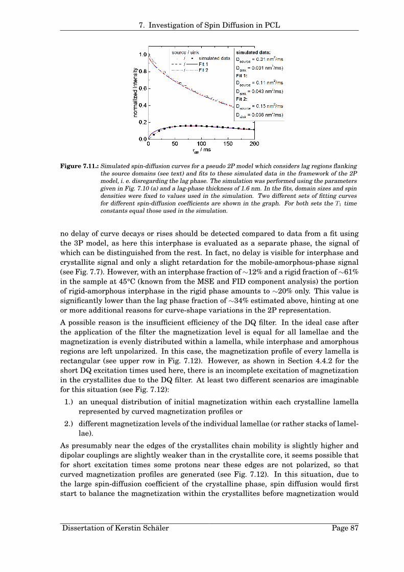
7. Investigation of Spin Diffusion in PCL
Figure 7.11.: Simulated spin-diffusion curves for a pseudo 2P model which considers lag regions flankingthe source domains (see text) and fits to these simulated data in the framework of the 2Pmodel, i. e. disregarding the lag phase. The simulation was performed using the parametersgiven in Fig. 7.10 (a) and a lag-phase thickness of 1.6 nm. In the fits, domain sizes and spindensities were fixed to values used in the simulation. Two different sets of fitting curvesfor different spin-diffusion coefficients are shown in the graph. For both sets the T1 timeconstants equal those used in the simulation.
no delay of curve decays or rises should be detected compared to data from a fit usingthe 3P model, as here this interphase is evaluated as a separate phase, the signal ofwhich can be distinguished from the rest. In fact, no delay is visible for interphase andcrystallite signal and only a slight retardation for the mobile-amorphous-phase signal(see Fig. 7.7). However, with an interphase fraction of∼12% and a rigid fraction of∼61%in the sample at 45°C (known from the MSE and FID component analysis) the portionof rigid-amorphous interphase in the rigid phase amounts to ∼20% only. This value issignificantly lower than the lag phase fraction of ∼34% estimated above, hinting at oneor more additional reasons for curve-shape variations in the 2P representation.
A possible reason is the insufficient efficiency of the DQ filter. In the ideal case afterthe application of the filter the magnetization level is equal for all lamellae and themagnetization is evenly distributed within a lamella, while interphase and amorphousregions are left unpolarized. In this case, the magnetization profile of every lamella isrectangular (see upper row in Fig. 7.12). However, as shown in Section 4.4.2 for theshort DQ excitation times used here, there is an incomplete excitation of magnetizationin the crystallites due to the DQ filter. At least two different scenarios are imaginablefor this situation (see Fig. 7.12):
1.) an unequal distribution of initial magnetization within each crystalline lamellarepresented by curved magnetization profiles or
2.) different magnetization levels of the individual lamellae (or rather stacks of lamel-lae).
As presumably near the edges of the crystallites chain mobility is slightly higher anddipolar couplings are slightly weaker than in the crystallite core, it seems possible thatfor short excitation times some protons near these edges are not polarized, so thatcurved magnetization profiles are generated (see Fig. 7.12). In this situation, due tothe large spin-diffusion coefficient of the crystalline phase, spin diffusion would firststart to balance the magnetization within the crystallites before magnetization would
Dissertation of Kerstin Schäler Page 87

7. Investigation of Spin Diffusion in PCL
Figure 7.12.: Schematic drawing of possible initial magnetization profiles after application of a DQ filterto semicrystalline PCL. Crystalline, interphase and amorphous domains are labeled c, i anda, respectively. The rectangular profiles in the upper part represent the ideal situation. Fil-ter ineffectiveness might lead to curved profiles (central picture) or unequal magnetizationlevels in individual lamellae (lower part). The sketch in the lower part represents a muchsimplified situation, as in reality the magnetization level will rather deviate between wholestacks of lamellae than between the lamellae within one stack (see Section 4.4.2). The arrowsdepict the spin-diffusion process locally differing in strength for the different scenarios.
be transferred further into the interphase and mobile-amorphous phase. Hence, ini-tially non-polarized outer regions of the lamellae should act as a crystalline lag phase,inducing a delayed decay of the crystallite signal and a retarded rise of the interphaseand mobile-amorphous phase signal compared to a scenario without lag phase. How-ever, the fit curves for the 3P model match well the experimental data of interphase andcrystalline phase and a delay is not observed. Furthermore, as discussed in Section 4.4.2the magnetization does not equilibrate within the crystallites as it should in accordancewith the argumentation given above. Therefore, either effects of such curved initialmagnetization profiles within the lamellae are very small or superimposed by other ef-fects.
The simulation model assumes that all lamellae initially exhibit the same level of mag-netization. Yet, as explicated in Section 4.4.2, the initial magnetization level rathervariates from stack to stack. Hence, interphase and mobile-amorphous regions close toless polarized lamellae will initially obtain less magnetization via spin diffusion thansuch near more strongly polarized lamellae and compared to a system with equal initialmagnetization of each lamella, changes in the shape of the spin-diffusion curves are ex-pected. Whether this effect can induce curve shapes similar to those discussed above forthe 2P model remains to be clarified by simulations of the scenario.
Magnetization Transfer Lags in Mobile-Amorphous PCL Domains. The delayedinitial rise and decay of sink and source signal from MAPE-filtered spin-diffusion mea-surements is expectedly reproduced well by simulations for the 2P model under consid-eration of a mobile lag phase (see Fig. 7.13).
The MAPE filter action is based on the fact, that signal of protons cannot be refocusedwhen the filter duration largely exceeds the inverse dipolar coupling strength betweenthem, i. e. when the couplings are too strong. As there is a gradient of chain mobilities
Dissertation of Kerstin Schäler Page 88

7. Investigation of Spin Diffusion in PCL
Figure 7.13.: Comparison of experimental spin-diffusion data with simulations using the pseudo 2P model,considering lag-phase regions flanking the source domains, for two different sets of spin-diffusion coefficients. The simulations were performed using the total thickness, T1 andspin-density parameters given in Fig. 7.10 and assuming a magnetization lag phase of 34%and 15% of the total rigid phase and mobile-amorphous phase, respectively.
and dipolar coupling strengths within the mobile-amorphous phase (see Section 4.4.1),ranging from strong couplings near the interphase to weak couplings in the middle ofthe domains, a too long filter in fact screens magnetization from protons at the edges ofthe amorphous domains. A similar effect is known for the Goldman-Shen filter sequence[113,117,151]. Furthermore, also technical imperfections and molecular motions on thetime scale of the sequence length may induce signal loss.
The fraction of mobile-amorphous-phase signal which is lost due to the filter can beestimated by comparing the corresponding signal intensities from an unfiltered anda MAPE-filtered MSE experiment. In the measurements for PCL at 45°C the lossamounted to 7% of the total mobile-amorphous-phase signal. Signals arising from thisnon-polarized fraction are not distinguishable from the rest of the mobile-amorphous-phase signal due to very similar signal-shape parameters. Therefore, this loss fractionacts as a typical magnetization lag phase (cf. Ref. [8]). Yet, a good agreement betweenmeasured and simulated spin-diffusion data was only reached for 15% of lag-phase con-tent within the mobile-amorphous phase (see Fig. 7.13).
Summarizing the above, the shift in initial rise and decay of the experimental spin-diffusion curves compared to simulated ones for the 2P model can quantitatively beexplained by the existence of a rigid and a mobile-amorphous magnetization lag phase.However, in both cases the estimated lag-phase fractions are significantly larger thanthe directly evident reasons suggest. In presence of such lag phases the spin-diffusioncoefficients determined from fitting the data using the 2P model deviate from the trueones. Furthermore, the discrepancy between the sets of spin-diffusion coefficients re-quired to describe the experimental curves from DQ-filtered and MAPE-filtered experi-ments does not vanish when lag phases are considered. Still the description of MAPE-filtered spin-diffusion data requires higher values of Da and Drig than necessary to char-acterize the corresponding DQ-filtered spin-diffusion data (see Fig. 7.13).
Dissertation of Kerstin Schäler Page 89

7. Investigation of Spin Diffusion in PCL
7.5. Effects of Corrugated Crystalline-Interphase Boundary Surfaces
Even when taking into account possible lag phase effects (and domain-size distributions,see Appendix F.4) in PCL, discrepancies persist between the measured spin-diffusiondata and the fit curves which still could not be interpreted (see Sections 7.3 and 7.4).In this section, a model of corrugated crystallite surfaces will be discussed qualitatively,which may yield a conceivable explanation of these mismatches.
As shown in Fig. 7.6 the 3P model for fitting the spin-diffusion data assumes pla-nar interfaces between the three polymer domains. However, in literature also roughcrystallite surfaces have been debated [20, 228, 255–257] or morphologies where rigid-amorphous and mobile-amorphous domains both have direct contact with crystallinematerial [119]. In the scenario discussed here, crystalline lamellae form protuberancestowards the mobile-amorphous phase at their edges, as shown in Fig. 7.14.8
(a) (b)
Figure 7.14.: Schematic representation of the domain morphology of a semicrystalline polymers consistingof crystalline lamellae, mobile-amorphous regions and rigid-amorphous interphase domainsin between, denoted c, a and i, respectively: (a) model with planar boundary surfaces and (b)model with corrugated crystallite surface.
In this scenario, polymer chains in the dents between such crystalline protuberancesand on the top of them are subject to mobility restrictions because they are fixed in thecrystallite at one end. They would therefore be evaluated as rigid-amorphous interphasematerial in NMR time-domain measurements. At a certain distance from the crystallitesurface the chain mobility is largely isotropic, so that the corresponding material canbe referred to as mobile-amorphous. Compared to the model with planar interfaces,in this scenario the crystallite surface is enlarged and the minimum distance betweencrystallite surface and the boundary of the mobile-amorphous domains is reduced (seeFig. 7.14), causing distinct changes in the magnetization development in a spin-diffusionexperiment, which are addressed in the following.
Consequences of Corrugated Crystallite Surfaces on Crystalline-Phase-Select-ed Spin-Diffusion Experiments. The shape of the contact area between the poly-mer domains enters the spin-diffusion equation in form of the dimension parameterk. As known from literature, changes of this parameter may affect the spin-diffusioncurves [89, 101, 250]. Due to the corrugated crystallite surface the geometry of thespin-diffusion process in a crystalline-phase-selected experiment is fractal with a di-mension parameter k ranging between 1 and 2 instead of k = 1 for the scenario withplanar interfaces. Following from Eq. 4.12, magnetization is transferred slightly fasterfrom the crystallites to the interphase via the enlarged boundary surface, resulting in
8Of course, also other forms of rough crystallite surfaces can be imagined.
Dissertation of Kerstin Schäler Page 90

7. Investigation of Spin Diffusion in PCL
a somewhat earlier decay and rise of the crystalline and interphase signal, respectively,compared to the curves obtained for a model with planar interfaces.
By contrast with the data from a fit using the 3P model, there is no accelerated intensityrise or decay of the measured crystalline-phase and interphase signal, although such amagnetization development could not be compensated by the fit. However, in Section 7.4ineffective DQ-filter action in the crystallites was discussed as a possible reason for afurther magnetization transfer lag inducing a retarded decay and rise of the crystallineand interphase signal, respectively. Also this effect was not visible in the experimentaldata, although it probably exists. Possibly, here both influences cancel each other, leav-ing the rise or decay times of the measured data in fair agreement with those from thefits. For a final clarification of the issue simulations for a scenario taking into accountcorrugated crystallite surfaces and a lack in filter efficiency are required.
Consequences of Corrugated Crystallite Surfaces on Amorphous-Phase-Select-ed Spin-Diffusion Experiments. The presumed effects of a corrugated crystallitesurface are complex in case of spin diffusion starting from the mobile-amorphous phase.They are demonstrated in Fig. 7.15. Here, magnetization flows to the interphase first,enabling a slight and early rise of the interphase signal intensity. However, at spotswhere the interphase is thin magnetization is preferably and rapidly transferred fur-ther to the crystalline domains with its efficient spin diffusion due to the strong dipolarcouplings. Therefore, the crystalline-phase and interphase signal grow almost simulta-neously. The magnetization also disperses within the interphase albeit less efficientlythan in the crystallites. The interphase signal therefore increases further, but with asmaller slope than present for the crystalline-phase signal. When magnetization has’filled up’ the crystalline protuberances, it seems possible that it is transferred back tostill non-polarized interphase material, resulting in a stronger second rise of the inter-phase signal. Due to their strong dipolar couplings the crystalline protuberances canremove more magnetization from the crystalline-interphase boundary and distribute itwithin the crystallites than the interphase could do at the same place in case of pla-nar surface boundaries. This suction action of the crystalline phase on magnetizationassumedly enables a higher crystalline-phase intensity at short mixing times than cal-culated for planar boundary surfaces, but at the expense of the interphase signal inten-sity.9 All these effects described here have actually been detected in the experimentalPCL data (see Figs. 7.7 (b) and 7.8).
Resulting from the strongly delayed and reduced rise of the interphase signal, being apart of the rigid-phase signal, a retarded increase of the latter is conceivable in the 2Pmodel compared to the scenario with planar interfaces. This effect could constitute theadditional magnetization transfer lag needed to finally explain the spin-diffusion datafrom the MAPE-filtered experiment for the 2P model.
Importantly, the discrepancy between the signal intensities of the sink curves from DQ-filtered and MAPE-filtered spin-diffusion experiments can finally be elucidated by tak-
9By contrast, the decreased minimum distance between crystalline and mobile-amorphous domainsis not expected to accelerate the rise of the mobile-amorphous-phase signal in a crystalline-phase-selected experiment significantly because magnetization is transported less efficiently within themobile-amorphous phase than within the interphase with its higher coupling strength and diffusioncoefficient.
Dissertation of Kerstin Schäler Page 91

7. Investigation of Spin Diffusion in PCL
Figure 7.15.: Demonstration of the effects of corrugated crystallite surfaces on the spin-diffusion curvesfrom a mobile-amorphous-phase-selected experiment. Direction and strength of the spin-diffusion process are indicated by green and claret arrows for scenarios with planar inter-faces (left) and corrugated crystallite surface (middle), respectively. Expected spin-diffusioncurves for both scenarios are sketched on the right using the same colour code.
ing into account corrugated crystallite surfaces and T1 relaxation. Because of rather fastT1 relaxation in the mobile-amorphous phase and the interphase and the slow relaxationin the crystallites, a faster magnetization transfer from the mobile phase into the crys-talline phase, as described above, partly prevents magnetization from being lost due torelaxation. Therefore the maximum signal intensity of the crystalline phase grows addi-tionally compared to the situation for planar interphases and the total increase exceedsthe signal loss in the interphase due to the simple redistribution of magnetization (seeabove). Thus, also the maximum intensity of the rigid-phase signal exceeds the valuereached in a simulation for a 2P model with planar surface boundaries.
Ignoring corrugated crystallite surfaces, enlarged intensities from a mobile-amorphous-phase-selected experiment are evaluated as resulting from enhanced spin diffusion com-pared to crystalline-phase-selected measurements where no such increase in sink inten-sity is expected.10 Hence, fitting such spin-diffusion data using the program describedin Section 7.3 with fixed domain-thickness parameters is not possible with one set ofspin-diffusion coefficients for both sets of data. To reproduce the enlarged sink intensityin the mobile-phase-selected experiment the fit yields a higher value of Da (and possiblyalso of Drig) than for the crystalline-phase-selected experiment, and in the 3P model anincreased value of Di or Dc is needed to additionally compensate the elevated simulatedinterphase signal intensity arising from the raise in Da.
In summary, the discrepancies between measured and simulated spin-diffusion data canbe explained qualitatively by the existence of corrugated crystallite surfaces in PCL.For a final clarification, however, a comparison of the individual scenarios by numericalsimulations is necessary. First tests indicate, that a simultaneous rise of crystalline andinterphase signal can be explained by a corrugated interface in fact [159].
10As the slow T1 relaxation in the crystalline phase does not cause much signal loss within the first tensof milliseconds of spin diffusion, the faster magnetization transfer due to the corrugated boundary ina crystalline-phase-selected experiment is not expected to affect the intensity of the interphase andmobile-amorphous-phase signal curves compared to the scenario with planar boundary surfaces.
Dissertation of Kerstin Schäler Page 92

7. Investigation of Spin Diffusion in PCL
7.6. Quantitative Results from Fitting PCL Spin-Diffusion Data
Despite the described discrepancies between measured and simulated spin-diffusioncurves, the measured data were analyzed in order to obtain spin-diffusion coefficientsfor PCL, which shall later on be used to derive realistic PCL domain sizes from spin-diffusion experiments in practice (see Chapter 8).
The considerations in Section 7.5 confirmed that mainly data from MAPE-filtered exper-iments pose a problem to the analysis, when using a fit model for three polymer phaseswith planar interfaces between them (3P model). Therefore the quantitative evaluationhas been restricted to data from DQ-filtered spin-diffusion and Saturation-Recovery ex-periments. Information about the implementation of the fit is given in Section 7.3. Thefit quality was fairly good in general (see Fig. 7.16). However, slight systematic devia-tions between measured data and the fit curves persisted, assumedly as a consequenceof domain thickness distributions (see Appendix F.4).
(a) (b)
Figure 7.16.: DQ-filtered spin-diffusion data (a) and Saturation-Recovery data (b) in comparison to curvesobtained from a simultaneous fit to both sets of data. Exemplarily, data from step C (at 27°C)and A (at 45°C) in the measurement program are plotted.
As it turned out that the fit results partially depend on the initial parameter values,three fits have been performed to data from each of the steps A to E in the measure-ment program with different initial values. In principle, in the fits the spin-diffusioncoefficient Di of the interphase could have been fixed to the average of the coefficientsof crystalline and mobile-amorphous phase because the spin-diffusion curves do not re-spond sensitively to changes of Di (see also Ref. [95]). Nontheless, in order to test thepossible parameter variations, Di was kept as a free parameter, here. During the fittingruns the parameter values possibly had to be reset, if physically unlikely combinationsof values arose as a result of domain-size distributions (see Appendix F.4). At the endof each fitting run the domain sizes were allowed to adjust freely in order to optimizethe fit quality. The thickness values obtained this way ranged within the margin of un-certainty of the thicknesses calculated from the SAXS long period L in each case. Theparameter values derived from the fits are summarized in Table 7.1.
Dissertation of Kerstin Schäler Page 93

7. Investigation of Spin Diffusion in PCL
step A step B step C step D step E45°C 45°C 27°C 27°C 45°C
fa 0.403±0.010 0.393±0.010 0.343±0.010 0.326±0.010 0.381±0.010fi 0.112±0.010 0.129±0.010 0.139±0.010 0.144±0.010 0.127±0.010fc 0.485±0.010 0.478±0.010 0.518±0.010 0.530±0.010 0.492±0.010
LSAXS/ nm 15.83± 0.30 15.80± 0.30 15.13± 0.30 14.99± 0.30 15.78± 0.30da,SAXS/ nm 6.57± 0.42 6.40± 0.42 5.38± 0.35 5.07± 0.33 6.20± 0.40di,SAXS/ nm 0.89± 0.12 1.02± 0.13 1.06± 0.14 1.08± 0.14 1.00± 0.13dc,SAXS/ nm 7.48± 0.45 7.34± 0.44 7.65± 0.46 7.77± 0.47 7.55± 0.45σrel,c 0.10 0.10 0.13 0.13 0.10σrel,a 0.51 0.51 0.48 0.48 0.50
da,NMR/ nm 6.59± 0.01 6.43± 0.01 5.36± 0.01 5.10± 0.04 6.22± 0.02di,NMR/ nm 0.90± 0.01 1.02± 0.01 1.06± 0.01 1.09± 0.01 1.01± 0.01dc,NMR/ nm 7.53± 0.02 7.32± 0.02 7.66± 0.01 7.76± 0.01 7.56± 0.01
T1a/ ms 89± 2 93± 2 62± 1 54± 2 88± 3T1i/ ms 214± 100 132± 10 87± 10 120± 20 134± 10T1c/ ms 595± 160 683± 20 423± 35 484± 30 753± 120
Da/ nm2ms−1 0.031±0.001 0.029±0.001 0.032±0.002 0.0344±0.0003 0.030±0.001Di/ nm2ms−1 0.179±0.016 0.209±0.062 0.160±0.035 0.210±0.024 0.206±0.031Dc/ nm2ms−1 0.308±0.055 0.375±0.058 0.330±0.076 0.279±0.028 0.358±0.054
Table 7.1.: Summary of results from NMR and SAXS measurements for all 5 steps in the temperatureprogram (see Fig. 7.1): Sample fractions f from NMR MSE measurements, long periods L fromSAXS, mean domain thicknesses dSAXS calculated from L via Eq. 7.3 using proton spin densitiesfrom Table E.1, relative distribution widths σrel = σ/dSAXS of domain sizes from SAXS (seeAppendix F.4) and domain thicknesses dNMR, T1 relaxation time constants and spin-diffusioncoefficients D from fitting the NMR spin-diffusion data (see text). The subscripts a, i and cdenote the mobile-amorphous phase, interphase and crystalline phase, respectively.
Spin-Diffusion Coefficient of the Mobile-Amorphous Phase. The spin-diffusioncoefficient Da could be determined from the fits with little scatter.11 No effect of sec-ondary crystallization was seen, but expectedly Da increased slightly and reversiblywith falling temperature because of increasing chain mobility and hence rising strengthof the residual dipolar couplings which mediate spin diffusion (see Fig. 7.17 (a)). Theabsolute change of Da from (0.030 ± 0.003) nm2/ms at 45°C to (0.033 ± 0.003) nm2/msat 27°C was low, however, compared to variations in the order of ∼0.012 nm2/ms de-termined for PB by Spiegel et al. for an equivalent temperature change [120]. In thetemperature range between 27°C and 45°C the value of Da is found by a linear fit yield-ing Da = ((-1.7 ± 3.0)·10-4 T [°C] + (0.0375 ± 0.012)) nm2/ms.
For PCL similar, yet slightly smaller spin-diffusion coefficients are expected than forNylon-6 (see Section 7.1) amounting to 0.034 nm2/ms to 0.084 nm2/ms as calculatedfrom the NMR proton line width at room temperature by Buda et al. [95, 97]. In fact,this expectation is confirmed here. Literature data for Da in PE (0.07 nm2/ms to 0.25nm2/ms) are larger than those obtained here for PCL. Furthermore, the values given for
11Due to domain-thickness distributions within the sample the magnetization transfer is presumablystronger locally than determined in the fits. At 45°C instead of Da ≈ 0.030 nm2/ms it rather amountsto a true value of ∼ 0.045 nm2/ms (see Appendix F.4).
Dissertation of Kerstin Schäler Page 94

7. Investigation of Spin Diffusion in PCL
(a) (b)
Figure 7.17.: Spin-diffusion coefficients Da, Dc and Di of the mobile-amorphous phase (a) and the crys-talline phase and interphase (b), obained from simultaneous fits to Saturation-Recoverycurves and spin-diffusion curves from DQ-filtered experiments for PCL, as a function of thetime in the measurement program (see Section 7.2). Results from fits with different initialparameters are plotted for every measurement step.
mobile-amorphous PCL at room temperature by Voda et al. [101] (Da = 0.14 nm2/ms to0.25 nm2/ms) exceed the results presented herein by a factor of 4 to 7, whereas investi-gations on local spin diffusion within the mobile-amorphous PCL phase at 45°C ,using ahole-burning technique, yielded only half the value obtained here [258], supposedly be-cause at this very local scale (∼1 nm) the geometry of the process is different comparedto the scenario assumed for the low-field measurements (see Section 7.1).
The trend of rising dipolar coupling strength with falling temperature is visible in thedevelopment of the T2 relaxation time constant as expected.12 However, the absolutevalues of Da calculated by help of T2 exceed the ones derived from the fit significantly(see Table 7.2). The calibration of Mellinger et al. [251] yields values which are approx-imately 10 times larger than Da from the fit. Anyway, this calibration cannot be usedhere, because it is based on a reference value obtained from NMR measurements underMAS (see Section 7.1). Yet, after scaling down the values derived from this calibrationby a factor of (0.76 ± 0.05) to adapt them to results from static NMR measurements assuggested in Ref. [156], they are still too large by a factor of 8 to 9. Also by computingDa from the T2 relaxation time constant via Eq. 7.2, a factor of 4 to 5 persists.13 Thesefindings indicate, that the stated relations of T2 and Da do not hold true in general formobile polymer phases. Compared to soft PI or PB blocks in block copolymers the amor-phous PCL phase exhibits considerably reduced spin diffusion [156, 251]. A possiblereason could be an effective obstruction of the magnetization transfer in direction of thechain backbone due to the COO group in the PCL repeat unit.
Spin-Diffusion Coefficients of Crystalline Phase and Interphase. The spin-diff-usion coefficients of crystalline phase, interphase and rigid phase derived from the fit
12T2 relaxation time constants were measured using the CPMG and Hahn-echo sequence. The results ofboth kinds of experiments were in good agreement.
13However, the value used here for the mean-squared distance 〈r2〉 between the nearest spins mightbe inappropriate as it was calculated by Voda et al. for PCL as a soft segment of a thermoplasticpolyurethane [101].
Dissertation of Kerstin Schäler Page 95

7. Investigation of Spin Diffusion in PCL
step A step B step C step D step E45°C 45°C 27°C 27°C 45°C
T2a / ms 0.68 0.63 0.48 0.46 0.60Da,calc / nm2 ms−1 0.326 a 0.331 a 0.353 a 0.357 a 0.334 a
0.248 b 0.252 b 0.268 b 0.271 b 0.254 b
0.123 c 0.133 c 0.173 c 0.181 c 0.139 c
Da,fit / nm2 ms−1 0.031±0.001 0.029±0.001 0.032±0.002 0.0344±0.0003 0.030±0.001
M2 / (2π)2 kHz2 290 291 303 301 292
Dc,calc / nm2 ms−1 0.423 d 0.424 d 0.432 d 0.431 d 0.425 d
Dc,fit / nm2 ms−1 0.308±0.055 0.375±0.058 0.330±0.076 0.279±0.028 0.358±0.054
a calculated using the calibration of Mellinger et al. [251];b as a but scaled down by a factor of 0.76 as suggested in Ref. [156];c calculated via Eq. 7.2 with 〈r2〉 = (0.29)2 nm2, adopted from Ref. [101];d calculated from the second moment M2 of the line shape of the crystalline-phase signal viaEq. 7.1.
Table 7.2.: Comparison of calculated spin-diffusion coefficients (subscript calc) of the mobile-amorphous(subscript a) and crystalline (subscript c) phase of PCL and the corresponding values derivedin the fit (subscript fit) for all steps in the measurement program.
amount to Dc = (0.34 ± 0.09) nm2/ms, Di = (0.19 ± 0.08) nm2/ms and Drig = (0.31± 0.09) nm2/ms, the latter being calculated as a weighted average of Dc and Di ac-cording to Eq. 7.5. Following from these results, the spin-diffusion coefficient of therigid-amorphous interphase can be fixed in the fits to the average of Dc and Da withouthesitation. Values of Dc for Nylon-6 [95, 97] (0.21 nm2/ms to 0.29 nm2/ms) are at thelower limit of the uncertainty range of values obtained from the fit, while those com-puted from the second moment M2 of the line shape of the crystalline-phase signal14 viaEq. 7.1 are at or above the upper limit (see Table 7.2). Due to the slight temperaturedependence of M2 (see Section 5.1) a decrease of Dc by about 0.008 nm2/ms was expectedfor a temperature change from 45°C to 27°C. However, the fit results scatter by up to0.09 nm2/ms (see Fig. 7.17 (b)) rendering such a small deviation indetectable.
The widely accepted value of the spin-diffusion coefficient in glassy PS reported byClauss et al. ((0.8 ± 0.2) nm2/ms) [139], which is frequently considered to be specific forrigid organic matter but was determined from measurements under MAS, significantlyexceeds the value obtained here for PCL crystallites. Yet, the corresponding value fromstatic low-field experiments ((0.38 ± 0.06) nm2/ms [156]) matches the PCL value withinthe uncertainty range. Furthermore, the parameter value determined here lies withinthe wide range of literature values for the crystalline phase of PE (0.11 nm2/ms to 0.83nm2/ms, see Section 7.1). Expectedly, as already reported for the amorphous PCL phase,investigations on local spin diffusion yielded a much smaller spin-diffusion coefficent inthe crystallites ((0.08 ± 0.02) nm2/ms) than found here (see above and Section 7.1).
Results on T1 Relaxation Time Constants. The fits yield stable and well-defined T1values only for the mobile-amorphous phase, where the longitudinal relaxation proceeds
14The second moment M2 of the line shape for the PCL crystallites was deduced from fits to the MSE data(see Section 4.1).
Dissertation of Kerstin Schäler Page 96

7. Investigation of Spin Diffusion in PCL
much faster than the spin diffusion: T1a � d2a/Da ≈ 1370 ms. The T1a values are in goodagreement with those from a linear fit to the initial rise of the corresponding Saturation-Recovery curves (see Section 5.1) and thus are supposed to be close to the true values.
The relaxation time constants T1c and T1i of the crystalline phase and interphase arelarger than T1a (see Table 7.1). Here the ratio between the T1 relaxation time and thecharacteristic spin-diffusion time d2/D is in the range of 15 to 25 for the interphase and3 to 4 for the crystalline phase. Thus, spin diffusion dominates within these phases.Supposedly due to domain-size distributions in the sample, the fits allow a multitude ofdifferent combinations of values for T1c and T1i (see Appendix F.4). The actual fit valuesdepend on the inital T1 parameter setting. True T1 values of these phases thereforecannot be given.15 As already described in Section 5.1 all three T1 times decrease withfalling temperature. Yet, no change due to proceeding secondary crystallization can beseen i. e. the very fast local dynamics in the sample are not influenced appreciably dueto this process.
In summary by means of simultaneously fitting data from DQ-filtered spin-diffusionand Saturation-Recovery experiments the effective spin-diffusion coefficient and the T1time of the mobile-amorphous phase could be determined with high accuracy. The corre-sponding values of the other two phases scatter strongly. Nevertheless average valueswere obtained for the parameters of these phases as well. While expectedly a tem-perature trend for the spin-diffusion coefficient of the mobile-amorphous was found,such a tendency could not be confirmed for the coefficients of the interphase, crystallinephase and rigid phase owing to the large scatter of these parameters. The value of theamorphous-phase spin-diffusion coefficient of PCL is in agreement with those knownfrom literature for Nylon-6 but is significantly lower than those calculated from pro-ton T2 relaxation times or line widths and the spin-diffusion coefficient of the crystallinePCL phase lies within the range of literature values for rigid polymer phases from staticlow-field experiments.
7.7. Initial Rate Approximation for the Estimation of Domain Sizes inPCL
As an alternative to complex computations the Initial Rate Approximation (IRA) pro-vides a simple, fast and widely used approach to estimate domain sizes in heteroge-neous polymer systems from spin-diffusion curves without requiring exact knowledgeof the structure of the system (i. e. the dimensionality of the magnetization trans-fer) [17, 93, 94, 96, 99, 104, 105, 110–112, 127, 128, 130, 139, 251]. Basically, the approachrelies on the idea that in a spin-diffusion experiment only a small layer around the in-terface between magnetization source and sink is affected by the magnetization transferat short mixing times τdiff. Because the sink region is much larger than this layer, asa short-time approximation one can assume a scenario of a finite source region, fromwhich magnetization is transferred into an infinite sink region [143]. For this situationan analytical solution of the spin-diffusion equation exists, from which an expression for
15The T1 data shown in Table 7.1 were obtained using characteristic time constants from a linear fit to theinitial rise of the Saturation-Recovery curves as initial values for the simultaneous fit of spin-diffusionand Saturation-Recovery data.
Dissertation of Kerstin Schäler Page 97

7. Investigation of Spin Diffusion in PCL
the source domain size can be deduced:
dsource = 2r0 =4√π
√DA√DB(
%H,A%H,B
√DA +
√DB
)√t0 (7.6)
Here, r0 denotes the position of the interface between source and sink domain and thesubscripts A and B designate the source and sink domain, respectively (see Fig. 7.18 (a)).In case the dimensionality of the spin-diffusion process differs from k = 1, a factor 4k
instead of 4 is used in Eq. 7.6. A derivation of this equation according to the consid-erations of Clauss et al. [139] is given in Appendix F.3, for a one-dimensional periodicstructure of alternating rigid and mobile-amorphous regions (2P model, see Section 7.3)of, e. g., a semicrystalline polymer.
(a) (b)
Figure 7.18.: Initial Rate approximation: (a) Magnetization profiles for the initial stages of spin diffusionfrom a magnetization source A at x < r0 to an infinite sink region B at x > r0. The arrowsdepict the evolution of the spin-diffusion process. The profile changes only in a small regionaround r0. (b) Spin-diffusion curves of source A and sink B in absence of T1 relaxation as afunction of the square-root of the mixing time τdiff. At the initial stage of spin diffusion thecurves can be approached by linear functions of
√τdiff. The characteristic value
√t0 can be
used to estimate r0 (see Eq. 7.6).
The parameter√t0 yields specific information about the speed of the spin-diffusion pro-
cess from the source to the sink domain. It is easily accessible from the spin-diffusioncurves in a √τdiff representation by performing a linear fit to the initial rise or decay ofthe sink or source curve, respectively (see Fig. 7.18 (b)). From the source domain sizedsource the thickness dsink of the sink domain can be found with the help of the massfractions and proton spin densities of the two phases as described by Eq. 7.4 for a one-dimensional spin-diffusion process. Due to the restriction of the considerations to themagnetization development at only one interface (see Appendix F.3) the IRA cannot beapplied directly to a 3P model, where two different kinds of interface exist. Yet, by sub-dividing one of the two phases in the 2P model, the calculation of domain sizes of thesub-phases from dsource or dsink is also possible using Eq. 7.4.
Eq. 7.6 was derived neglecting T1 relaxation. Thus, before it can be applied, data fromspin-diffusion measurements at low magnetic field, which are substantially influencedby T1 relaxation effects, have to be corrected correspondingly, e. g., by multiplicationby an exponential factor et/T1 [17]. But, as relaxation processes within source and sinkphase both affect the shape of the spin-diffusion curves, a correction with the T1 value
Dissertation of Kerstin Schäler Page 98

7. Investigation of Spin Diffusion in PCL
of only one of the phases is inadequate. Here, the corrections of the experimental datahave been performed by multiplying them by et/T1,ave,ini , with T1,ave,ini being a weightedaverage of the T1,ini time constants of all three phases in the sample, obtained fromlinear fits to the initial rise of the corresponding Saturation-Recovery curves: T1,ave,ini =
fcT1c,ini + fiT1i,ini + faT1a,ini. This parameter was chosen because the T1 relaxation in allPCL phases affects the experimental spin-diffusion data to a certain extent, presumablydepending on the corresponding phase fraction. T1,ave,ini amounted to about 240 ms to360 ms at 45°C and ∼140 ms at 27°C.
According to Mauri et al. the spin-diffusion sink curve is better suited for the initialrate approach than the source curve, as seemingly its shape depends less on the actualT1 value chosen for correction, the fit region and the experimental uncertainties [8].Following this suggestion, linear fits to the initial rise of the normalized and T1 correctedsink curves (as a function of √τdiff) from the spin-diffusion experiments for PCL and the2P model have been performed for all steps in the measurement program. An exampleis displayed in Fig. 7.19. Actually the sink curve shape is sigmoidal at very short mixingtimes τdiff due to magnetization transfer lags discussed in Section 7.4. Therefore the fitrange was adapted to cover only the region of the linear curve rise as recommendedby Mauri et al. [8]. The values of the parameter
√t0 obtained here are summarized in
Table 7.3. The uncertainties reported were determined by slightly varying the intervalboundaries for the linear fit.
Figure 7.19.: Experimental spin-diffusion curves for PCL at 45°C from a MAPE-filtered experiment andInitial Rate Approximation after T1 correction as described in the text.
Domain sizes were calculated for the one-dimensional spin-diffusion scenario from√t0
via Eq. 7.6 for the source domain and via Eq. 7.4 for the sink domain, using relativeproton spin densities given in Table E.1. The values of the spin-diffusion coefficientsrequired for the calculation were adopted from the simultaneous fits to the experimentaldata described in Sections 7.3 and 7.6. Here, for each step in the measurement programat least three triples of values (Da, Di, Dc) were used, for which a good fit of the spin-diffusion and Saturation-recovery data had been obtained. The diffusion coefficient ofthe rigid phase was estimated as a weighted average via Eq. 7.5. The domain sizesresulting from the IRA are summarized in Table 7.3. The uncertainties given in thetable arise from the uncertainties of
√t0 and the scatter of the spin-diffusion coefficients.
Dissertation of Kerstin Schäler Page 99

7. Investigation of Spin Diffusion in PCL
step A step B step C step D step E45°C 45°C 27°C 27°C 45°C
results from MAPE-filtered spin diffusion√t0/√
ms 20.4± 1.0 22.3± 1.0 15.3± 1.8 16.7± 1.4 18.4± 1.0da/nm 6.2± 0.4 6.7± 0.5 4.7± 0.7 5.2± 0.5 5.6± 0.4drig/nm 8.7± 0.6 9.8± 0.7 8.5± 1.4 10.3± 0.9 8.7± 0.7
results from DQ-filtered spin diffusion√t0/√
ms 33.0± 0.8 33.8± 0.6 33.6± 0.5 34.1± 0.5 23.8± 0.6da/nm 6.7± 0.3 6.6± 0.3 5.4± 0.3 5.2± 0.1 6.4± 0.3drig/nm 9.5± 0.4 9.6± 0.5 9.8± 0.5 10.1± 0.2 9.8± 0.4
results from SAXS
da/nm 6.6± 0.4 6.4± 0.4 5.4± 0.4 5.1± 0.3 6.2± 0.4drig/nm 9.3± 0.6 9.4± 0.6 9.8± 0.6 9.9± 0.6 9.6± 0.6
Table 7.3.: Results from Initial Rate Approximation performed for data from MAPE-filtered and DQ-filtered spin-diffusion experiments of PCL compared to domain sizes calculated from SAXSlong periods via Eq. 7.3 using proton spin densities from Table E.1. The subscripts a and rigdenote the mobile-amorphous and rigid phase, respectively.
Comparing the calculated values with true domain sizes derived from SAXS long peri-ods, the best agreement is found for thicknesses obtained from DQ-filtered spin-diffusionexperiments. Here the values from the IRA are slightly larger than the true ones by2% to 3% and the temperature trend is readily reproduced. As already pointed out inSection 7.5 data from the MAPE-filtered experiments cannot be described by a modelwith planar interfaces between the polymer domains. Consequently problems were alsoexpected when performing the IRA. In fact, the thickness results obtained from MAPE-filtered experiments are in worse agreement with the true values than those from theDQ-filtered measurements (see Table 7.3). Yet, the temperature trend of the mobile-amorphous-phase domain size is visible here as well.
Importantly, no agreement could be found between thicknesses derived from the SAXSlong period and those estimated via Eq. 7.6 using spin-diffusion coefficients of the mobile-amorphous phase which were calculated from proton T2 relaxation time constants or linewidths. Here, the domain sizes obtained from IRA are too large by a factor of about 2.
In summary, the Initial Rate Approximation yields domain sizes for PCL which matchwell the real values derived from SAXS long periods under the condition that
• only data from DQ-filtered experiments is analysed by IRA,
• the weighted average of T1,ini values of all three polymer phases, obtained fromlinear fits to the initial rise of the corresponding Saturation-Recovery curves, isused for T1 correction and
• the calculation of the average source domain size via Eq. 7.6 is accomplished withthe help of the spin-diffusion coefficient values given in Section 7.6 for measure-ment temperatures in the range of about 27°C to 45°C.
Dissertation of Kerstin Schäler Page 100

7. Investigation of Spin Diffusion in PCL
7.8. Summarizing Remarks
Generally solid-state 1H NMR spin-diffusion measurements are well-suited for the de-termination of domain sizes in semicrystalline polymers. In comparison to other tech-niques used for this purpose, in principle, they do not require any sample pretreatment,such as staining, as here differences in chain mobility between crystallites and amor-phous phase are exploited. Importantly, domain sizes in systems with about 50% crys-tallinity, which may pose problems to SAXS measurements due to overlying peaks, areaccessible by the help of spin-diffusion investigations.
However, difficulties arise in the case of low-field NMR due to phase-specific T1 relax-ation affecting the shape of the spin-diffusion curves in a complex way. In this work, thiseffect was accounted for in a numerical approach for solving the spin-diffusion equationfor two or three-phase morphologies using a simulation and fit program.
Furthermore a lack of knowledge about correct spin-diffusion coefficients in a distinctsample system complicates the determination of domain sizes. As information on spin-diffusion coefficients in PCL, the polymer system of choice here, has been rare, the aimwas to perform spin-diffusion experiments to identify these coefficients with the helpof domain thicknesses derived from SAXS measurements. By interpretating the spin-diffusion data interesting insights were gained:
• By examination of spin-diffusion data for PCL as a two-phase system, containingrigid and mobile-amorphous domains, magnetization transfer lags became evidentwhich partly result from the initially unpolarized interphase and signal loss due tothe MAPE filter. To prevent the former it is recommended to treat the interphaseas a separate phase using a three-phase model. Incomplete excitation of magneti-zation within the crystalline phase by the DQ filter is a further possible reason fora magnetization transfer lag.
• Non-planar, corrugated crystallite boundary surfaces can qualitatively offer expla-nations for
1.) the deviating shape of the spin-diffusion curves of the interphase measuredin MAPE-filtered experiments as compared to simulated data and
2.) the fact that stronger spin diffusion is detected from the mobile-amorphousphase to the crystallites via the interphase than vice versa.
Such non-planar interfaces may represent another reason for retarded magneti-zation transfer, detected for the 2P model. The quantitative clarification of thismatter by means of model simulations is the subject of ongoing work.
In order to determine spin-diffusion coefficients for PCL which are useable in prac-tice, solely DQ-filtered spin-diffusion and Saturation-Recovery data of crystalline phase,mobile-amorphous phase and interphase were simultaneously fitted. MAPE-filtereddata have been excluded from the analysis because of the considerable discrepanciesbetween the measured and simulated curves. The resulting coefficients amount to
• Da = ((-1.7 ± 3.0)· 10−4 T [°C] + (0.0375 ± 0.0120)) nm2/ms,
• Di = (0.19 ± 0.08) nm2/ms,
• Dc = (0.34 ± 0.09) nm2/ms and
• Drig = (0.31 ± 0.09) nm2/ms,
Dissertation of Kerstin Schäler Page 101

7. Investigation of Spin Diffusion in PCL
for temperatures of about 27°C to 45°C. Within the limits of uncertainty the coefficientDc of the crystalline phase is in good agreement with literature data obtained fromstatic low-field NMR measurements. Yet, the coefficient Da of the mobile-amorphousphase is significantly smaller than values calculated from line widths or T2 relaxationtimes, possibly due to COO groups in the PCL repeat units, obstructing an efficientmagnetization transfer along the chain backbone.
The domain sizes derived from SAXS long periods can be reproduced well by analyzingspin-diffusion data from DQ-filtered experiments by means of the Initial Rate Approx-imation, when T1 correction is realized by means of a weighted average of the T1 timeconstants of all three polymer phases, obtained from linear fits to the initial rise of thecorresponding Saturation-Recovery curves.
Dissertation of Kerstin Schäler Page 102

8. The Influence of Cyclic Chain Topology on PCL Dynamics and Crystallization
8. The Influence of Cyclic Chain Topology on PCLDynamics and Crystallization
In order to synthesize semicrystalline polymers which are adapted to particular pur-poses, it is necessary to obtain comprehensive knowledge about the effects of all pa-rameters influencing the developing semicrystalline structure. Yet, until now certainaspects of the polymer crystallization have remained indistinct, such as the influence ofchain topology and molecular weight as well as the role of the entanglements prior toand during crystallization [31–38,226,229,231].
In this context, the effect of chain topology on polymer crystallization and the formingsemicrystalline structure shall be elucidated here, by comparing cyclic polymer chainsand their linear analogues with the same number of repeat units with regard to chainmobility in the melt, crystal growth, crystallinity and crystal thickness. For this pur-pose the crystal-fixed polymer PCL was chosen as a model system, because mechanismsfor the synthesis of linear, cyclic and other PCL topologies are well-known [259–262]and the crystallization of the linear form has already been investigated intensively (seeSection 6 and Refs. [68,221,253,263,264]).
Cyclic polymers are supposed to adopt more compact conformations than linear chains[265–273]. They comprise double-folded loops and may be percolated by loops of neigh-boring chains [274,275]. Often ring polymers are depicted in a ’lattice-animal’ represen-tation, describing single rings moving in a lattice of immobile topological obstacles whichare formed by the neighboring chains [273]. Their specific topology turns cyclic polymersinto attractive model systems for the exploration of, e. g., effects of highly mobile chainends on chain dynamics and the physical properties of the material [275–279], reptationprocesses which seem to be unavailable for rings [275], percolation [280] or chain-foldingphenomena [281,282].
So far, theoretical investigations of cyclic chains have mostly been concerned with theconformation and the dynamics of rings in solution or in the melt [266, 267, 270–273,283–286]. A number of cyclic polymers have also been characterized experimentally upto now, such as cyclic PS and PB [275,277,278] and, in particular, cyclic PDMS for whichcomprehensive investigations have been performed by Semlyen and coworkers since the1960s [279, 287–294]. However, studies on macromolecular self-organization processes,e. g. the crystallization of cyclic polymers, are rare. Besides some DSC characteristics ofcyclic systems of high molecular weight [237, 261, 292], investigations of monodispersecyclic alkanes and poly(ethylene oxide)s of low and medium molecular weights havebeen reported [281, 282]. Yet, such systems exhibit almost perfect crystal structureswith closely packed and integer-folded chains and reach crystallinities close to 100%.Hence, they are not representative for highly entangled semicrystalline polymers.
Reports on PCL of different topologies mostly concentrated on polymer synthesis andthe determination of crystallization temperatures in DSC experiments [259,261,262]. Ingeneral they seem to indicate a reduction of the crystallization tendency with decreasinglarge-scale chain mobility and increasing steric hindrance of the individual polymerchains [260, 295]. Only recently new synthesis strategies enabled first attempts to amore detailed comparison of the crystallization behavior of linear and cyclic PCL oflow [296] and high [297] molecular weights by DSC, optical microscopy and SAXS.
Dissertation of Kerstin Schäler Page 103

8. The Influence of Cyclic Chain Topology on PCL Dynamics and Crystallization
Remarks on the Investigated Samples. In this chapter, the semicrystalline struc-ture of linear and comparable cyclic PCL chains at molecular weights Mn between28 kg/mol and 43 kg/mol, i. e. above the entanglement molecular weight Me of about3 kg/mol [298–300], and polydispersities between 1.6 and 2.1 as determined by Gel Per-meation Chromatography (GPC, see Appendix A and Table 8.1) is surveyed. The cyclicPCL chains were prepared by Dipl.-Chem. E. Ostas by insertion polymerization accord-ing to procedures reported by Kricheldorf et al. [301]. For the ring opening polymer-ization of ε-caprolactone, an Sn-based cyclic initiator was used which did not allow forthe concatenation of rings. The linear polymers were obtained from the respective cyclicPCLs directly, by cleavage of the Sn-O bond generated by the initiator. They were freeof tin and exhibited the same number of monomers as their cyclic counterparts. Moredetailed comments and details on sample synthesis are given in Appendix A.
GPC measurements (see Appendix A) revealed higher retention volumes and thus lowerapparent molecular weights for the cyclic PCLs as compared to their linear analogues(see Fig. 8.1), although equal molecular weights were to be expected.1 The reason forthis difference lies in the fact that GPC detects the hydrodynamic radius of the polymerchains. This radius is lower for a cyclic chain in comparison to its linear counterpartwith the same number of monomers, because linking both ends of a linear chain reducesthe overall dimensions of the chain [302]. Hence, the GPC results confirm the successfulsynthesis of rings.
Figure 8.1.: GPC traces for a pair of linear and correspond-ing cyclic PCL with indicated retention vol-ume. The apparent molecular weights result-ing from a calibration with PS standards andthe converted PCL molecular weights amount to63.4 kg/mol and 35.4 kg/mol for the linear PCLand 57.4 kg/mol and 32.1 kg/mol for the cyclicPCL, respectively (see Appendix A, plot adoptedfrom Ref. [242]).
Furthermore, results from GPC studies indicated a fast degradation of cyclic PCL in ahumid environment. Therefore, all measurements described here have been performedunder the exclusion of air and moisture and the samples have been stored under vac-uum. However, also linear chains decomposed when stored at high temperatures for alonger time. Details concerning the investigation of sample degradation are given inAppendix B.
In order to elucidate the connection between chain mobility and the semicrystallinestructure formed by the linear and cyclic PCL chains, first, results on chain mobilityin the melt are presented as obtained from 1H low-field NMR Hahn-echo and multiple-quantum experiments and supported by findings from rheological measurements. More-over a comparison is drawn between crystallinities, lamellar thicknesses and crystal-lization kinetics of the linear chains and their cyclic analogues as detected by 1H low-field NMR and DSC.
1The molecular weight of the initiator (233 g/mol), which was eliminated during the formation of linearchains from the cyclics, is within the GPC uncertainty.
Dissertation of Kerstin Schäler Page 104

8. The Influence of Cyclic Chain Topology on PCL Dynamics and Crystallization
8.1. Chain Mobility in the Melt
1H Low-Field NMR Hahn Echoes. In polymer melts a variety of molecular dy-namics takes place spanning a wide range of correlation times (see Chapter 2). Fast,random and almost isotropic segmental motions (Rouse modes) at motional rates farabove the proton dipolar coupling strength of about 20 kHz average the couplings toa large extent (see Section 3.3). Thus, in the ideal case these motions hardly causeany decay of the transverse magnetization, measured by means of the Hahn-echo se-quence [148]. Moreover, chain motions on the time scale of the Hahn-echo sequence,i. e. in the range of some milliseconds, hamper the signal refocusing and cause a slowdecay of the transverse magnetization with a rather long corresponding T2 relaxationtime constant [71,303].
However, for long polymer chains, with molecular weights above the entanglement limitMe, topological restrictions, posed by chain entanglements or other packing constraints,induce an anisotropy of the fast chain motions on the NMR time scale and a semi-local residual order of the chains. Thus, dipolar couplings are not averaged out com-pletely [40, 71] and the residual static dipolar couplings cause an additional (coherent)dephasing of the transverse magnetization detected in a Hahn-echo measurement [303].Hence, the investigation of the T2 relaxation of the transverse magnetization at temper-atures far above Tg can yield information about the density of topological constraints(e. g. entanglements) and/or the time scale of large-scale chain motion [40].
In order to compare the T2 relaxation behavior of the linear and cyclic PCL chains inthe melt (under exclusion of disturbing effects due to the inhomogeneity of the magneticfield), Hahn-echo decay curves have been measured at 80°C for samples which had beenkept at 90°C for approximately 30 minutes to avoid melt-memory or self-seeding effects(see Chapter 6) and were then transferred into the pre-heated spectrometer directly.The Hahn-echo decay curves are displayed in Fig. 8.2 for a pair of samples of linear andcorresponding cyclic chains with a molecular weight Mn,lin = 35.4 kg/mol of the linearform.
The initial non-exponential shape of the decay curves (see Fig. 8.2) implies dominat-ing effects of the residual dipolar couplings as expected for melts of polymers with amolecular weight above Me [71, 304]. An apparent T2 time constant was derived for ev-ery investigated sample as the time at which the Hahn-echo intensity had decayed to
Figure 8.2.: Relaxation curves of transversemagnetization for a pair of samplesof linear and corresponding cyclicPCL with Mn,lin = 35.4 kg/mol inthe melt at 80°C, measured bylow-field 1H NMR Hahn-echo ex-periments. The inset highlightsthe non-exponential initial shapeof the decay curves (graph adoptedfrom Ref. [242]).
Dissertation of Kerstin Schäler Page 105

8. The Influence of Cyclic Chain Topology on PCL Dynamics and Crystallization
a fraction of (1/e) of the initial intensity (see Fig. 8.2). The corresponding values aresummarized in Table 8.1.
As visible in Fig. 8.2 and Table 8.1, the T2 relaxation is faster for the linear PCL chainsthan for the cyclic ones. This difference indicates a stronger motional anisotropy inthe samples containing linear PCL as compared to the cyclic analogues. This strongeranisotropy may result from stronger or more frequent restrictions to the fast mobilityof the linear chains due to more or enhanced chain entanglements or a higher numberof packing constraints caused by neighboring chains compared to the cyclics.2 Yet, alsoa longer time required for isotropic large-scale motions of the linear chains could be thereason for this finding.
1H Low-Field Multiple-Quantum NMR. From Hahn-echo decay curves the infor-mation about the dephasing due to residual static dipolar couplings and about spin re-laxation induced by thermal motions on the time scale of the sequence length can hardlybe separated [40, 305]. Therefore, additionally 1H NMR multiple-quantum (MQ) exper-iments have been performed here for three sample pairs of linear and cyclic PCLs withmolecular weights Mn between 28.3 kg/mol and 42.9 kg/mol to study the chain mobilityin the molten state.
Typically, MQ NMR sequences are used for the determination of weak residual dipo-lar couplings in polymeric systems such as polymer melts and elastomers [40]. De-tails on the theoretical background and the applicability of the method as well as onthe experimental implementation and the data analysis are summarized elsewhere[40,41,306,307]. Here, a pulse sequence of variable duration τDQ (an advanced versionof an early MQ experiment of Baum and Pines [40]) was used to obtain a normalizeddouble-quantum build-up curve InDQ(τDQ), whose initial increase is related to the resid-ual dipolar coupling strength Dres as well as to the semi-local order in the sample andis independent of the time scale of segmental fluctuations.
As can be seen in Fig. 8.3 (a), build-up curves InDQ(τDQ) were received for linear andcyclic PCL, confirming again that residual local order is present in the samples.3 How-ever, the initial slope and intensity of the curves is larger for the linear chains comparedto the cyclic ones. (In the region of the steepest increase at τDQ ≈ 1 ms the intensity ratioamounts to about 2.5.) In agreement with the conclusions from the Hahn-echo measure-ments, this observation indicates stronger motional anisotropy and higher residual localorder in the samples consisting of linear PCL chains due to more or stronger hindrancesto fast chain mobility.
As longer chains tend to form more entanglements and induce a higher degree of mo-tional anisotropy, the build-up intensity exhibits a slight increase with rising molecularweight for the linear chains. Yet, the effect is weak for the narrow range of molecularweights studied here, where polydispersities larger than 1.6 cause a considerable over-lap of the molecular weight distributions. No molecular weight trend could be found forthe Hahn-echo relaxation curves. Presumably, it was masked there by dynamic effects
2From the polymer theoretical point of view, cyclics adopt collapsed conformations rather than formingentanglements in the conventional sense [283, 285]. Hence the term ‘packing constraint‘ seems morereasonable here.
3The intensities presented here are smaller than shown in Refs. [40, 41] because a tail subtraction asdescribed in these references has not been possible due to the polydispersity of the samples.
Dissertation of Kerstin Schäler Page 106

8. The Influence of Cyclic Chain Topology on PCL Dynamics and Crystallization
(a) (b)
Figure 8.3.: Results from 1H low-field multi-quantum NMR experiments at 80°C for samples of linearand corresponding cyclic PCL chains of different molecular weights given in the legend forthe linear PCL. (a) Normalized intensities InDQ as a function of the excitation time τDQ, (b)orientational autocorrelation function C(τDQ) of the second Legendre polynomial (in arbitraryunits), calculated from the data in (a). The dotted line represents a constructed autocorre-lation function for Z = 11 (see text) based on experimental data for PB, PI and PDMS fromRef. [41] with corresponding Doi-Edwards tube-model regimes indicated by Roman numerals.The label 0 designates subsegmental dynamics (graphs adopted from Ref. [242]).
due to motions of the dipolar coupling tensor [307]. The cyclic PCL chains do not exhibita molecular weight effect neither in the MQ measurements nor in the Hahn-echo exper-iments. Assumedly this is due to contaminations of the samples with small but differingamounts of linear chains (see below).
In the region of the initial curve rise the normalized intensity InDQ is directly related tothe orientation autocorrelation function C(t) of the second Legendre polynomial P2:
C(t) = 〈P2(cosθ(t)) · P2(cosθ(0))〉 ,
describing the loss of orientational memory of the chain segments, with θ being the angleof the segmental orientation relative to the external magnetic field [306]:
InDQ
τ2DQ∝ C(τDQ) ∝ D2
res .
In Fig. 8.3 (b) the autocorrelation functions C(τDQ) of the investigated samples are de-picted. For the linear PCL chains no significant deviations of the initial curve decays ofthe three samples have been found, hinting at a distribution of residual dipolar couplingstrengths Dres, probably as a consequence of polydispersity. The same can be concludeddirectly from the rather linear initial rise of the build-up curves in Fig. 8.3 (a). Bycontrast, for a single residual dipolar coupling strength an inverted Gaussian shape isexpected.
According to the Doi-Edwards tube model, the autocorrelation function C(τDQ) obeysa power law with specific scaling exponents for the different time regimes of polymerdynamics, ranging from free Rouse modes (regime I) at short correlation times in therange of nanoseconds via constrained Rouse dynamics (regime II) and chain reptation
Dissertation of Kerstin Schäler Page 107

8. The Influence of Cyclic Chain Topology on PCL Dynamics and Crystallization
(regime III) to free chain diffusion (regime IV) at correlation times between millisecondsand days [41,307]. As it is known from literature for a melt of linear chains, the scalingexponent adopts a value of -0.85 in regime I, which increases when passing over toentangled dynamics at the entanglement time τe [41, 308]. In the constrained-Rouseregime II the scaling exponent depends on the molecular weight of the polymer. Forthe investigated PCL samples with an average number Z of entanglements per chainbetween 6 and 14 (Z = Mn,lin/Me with Me ranging between 3 kg/mol and 5 kg/mol[298–300]) the regime-II exponent adopts values between -0.44 and -0.48 (cf. Ref. [41]).The correlation function decay steepens in regime III before passing over to regime IV(see Fig. 8.3 (b)), with the corresponding scaling exponent changing from -0.5 near theRouse time τR to -1.5 being reached at the disentanglement time τd [41].
For the linear PCL chains investigated herein the relaxation power law exponent ex-tracted from the autocorrelation functionC(τDQ) amounts to -0.77± 0.15 (see Fig. 8.3 (b)),the large uncertainty being caused by bad statistics for the small signal intensities. Theslope for the cyclics is slightly steeper, yet, the exponent (-0.82 ± 0.20) is similar to theone of the linear chains within the limits of uncertainty. The entanglement time τe ofthe linear PCL chains at 80°C can be estimated to be on the order of 10−3ms using therelation τe ' 4ταN
2e found for PB in Ref. [41], with τα being the α-relaxation time con-
stant at the measurement temperature and Ne naming the number of Kuhn segmentsbetween two entanglements. The time constant τα was extrapolated from the results ofdielectric measurements [167, 168] and Ne was estimated4 to range between 30 and 50with the help of the entanglement molecular weight Me (see above) and the Kuhn seg-ment length of PCL of 7 Å [309]. As the time range of our measurements is far beyondτe (see Fig. 8.3 (b)), the scaling exponent of -0.77 is related to the Doi-Edwards regimeIII, revealing the presence of reptation-like dynamics of the linear PCL chains at 80°C.
As the autocorrelation function C(t) is proportional to the time-dependent shear modu-lusG(t), the multi-quantum NMR data can be compared to rheology data from literaturedirectly. Conducting shear measurements of a melt of polystyrene rings of high molec-ular weight (Z between 8 and 11, Me ≈17.5 kg/mol,), in contrast to linear-chain stressrelaxation via reptation, Kapnistos et al. [275] found additional, faster relaxation modesfollowing a power law behavior. This finding has been confirmed recently by moleculardynamics simulations of Halverson et al. [285]. The stronger relaxation of the cyclicsdue to these additional modes is expressed in a lower stress-relaxation modulus of thecyclic PS as compared to corresponding linear chains at times larger than the entangle-ment relaxation time τe. In accordance with this finding the autocorrelation functionsof the cyclic PCLs are placed beneath the ones of the linear chains (see Fig. 8.3 (b)).However, according to theoretical and experimental results reported in literature theautocorrelation function should decay much faster for the melt of rings than for the lin-ear analogues [273, 275]. The similar scaling exponents obtained here again hint at acontamination of the melt of rings with linear chains (see below).
Rheological Investigations. The differences in the mechanical relaxation spectrumof PCL rings and linear chains are reflected in the frequency-dependent shear storageand loss moduli G′ and G′′ measured in rheological experiments (see Appendix A) in
4The estimated value is large as compared to the value Ne,PB '15 found for PB [41] with a similar Me, butstill it is in the same range.
Dissertation of Kerstin Schäler Page 108

8. The Influence of Cyclic Chain Topology on PCL Dynamics and Crystallization
the melt. As depicted in Fig. 8.4 (a) for a pair of PCL samples (Mn,lin = 35.4 kg/mol)at 60°C, the moduli of the cyclic polymer both are significantly lower than those of thecorresponding linear analogue. The coinciding log-log slopes of the shear moduli of bothsamples are consistent with the very similar power law exponents of their orientationautocorrelation functions (see above).
(a) (b)
(c)
Figure 8.4.: Results from rheological measurementsfor a sample pair of linear and cyclicPCL withMn,lin = 35.4 kg/mol measuredin the melt at 60°C. (a) Shear storagemodulus (G′) and loss modulus (G′′) asa function of the shear frequency ω. Thebroken lines correspond to linear andquadratic functions of ω according to theasymptotic limits for G′ and G′′. (b)Loss tangent tan δ and (c) melt viscosityη as calculated from (a) (graphs adoptedfrom Ref. [242]).
Although a cross-over point of G′ and G′′ could not be reached in the measurementsat the highest possible measurement frequency (ω = 100 rad/s),5 the values of the losstangent tan δ = G′′/G′ suggest that a crossover point (i. e. a frequency where tan δ = 1)exists not only for the linear chains but also for cyclic PCL (see Fig. 8.4 (a) and (b)). Yet,compared to the linear chains this point is shifted to higher frequencies for the cyclics,indicating higher flexibility and/or mobility of the cyclic chains enabling them to followthe fast shear motion in the high frequency range more easily.
For both samples the storage modulus G′ deviates from the expected asymptotic powerlaw behavior (see Fig. 8.4 (a)), presumably due to experimental imperfections or a dis-tribution of terminal relaxation times resulting from the polydispersity of the samples.However, the loss modulus G′′ approaches terminal flow behavior at low of shear fre-quencies ω, turning G′′ = η · ω into a direct measure for the melt viscosity η. The vis-cosities of both samples as obtained from the data in Fig. 8.4 (a) are given in Fig. 8.4 (c)
5A reduction of temperature in order to shift the crossover point to lower frequencies was not feasible dueto crystallization setting in at temperatures below 60°C.
Dissertation of Kerstin Schäler Page 109

8. The Influence of Cyclic Chain Topology on PCL Dynamics and Crystallization
as a function of ω (for numerical values see Table 8.1). The values for the PCL ringsare lower than for the linear form by almost a factor of two, confirming a higher flu-idity of the melt of rings due a faster mechanical relaxation as compared to the linearchains [275]. Similar trends have been found in theoretical [285] and experimentalworks, e. g., on PS [278,290,310] and on PB by Roovers [277]. Compared to the values ofthe linear counterparts the latter reported melt viscosities of the cyclics being reducedby a factor of 10. The smaller factor found here can be ascribed to contaminations ofthe ring systems with opened linear chains, the extent of which cannot be evaluateddefinitely. Yet, compared to viscosity data in Refs. [275, 311], the results obtained herehint at an impurity level of about 10%.
The melt rheology experiments were repeated for another pair of samples (Mn,lin =38.6 kg/mol) and for both sample pairs at a higher temperature of 80°C (see Table 8.1).All measurements yielded consistent results. In conclusion, the shear measurementdata are in good agreement with the findings from Hahn-echo and MQ NMR experi-ments, where a higher chain mobility was found for cyclic PCL as well.
8.2. Crystallinity and Crystallization
NMR and DSC Crystallinity Measurements. For crystallinity determination bymeans of low-field 1H NMR, sample pairs of linear and corresponding cyclic PCL chainswere kept at 90°C for about 30 minutes in order to remove melt-memory or self-seedingeffects (see Chapter 6) and then crystallized isothermally at Tc = 48°C all together in anexternal thermostat for four to five days (depending on the order of the subsequent NMRmeasurements) before they were directly transferred into the pre-heated spectrometer(48°C). Thus, the crystallization time was extended for the samples investigated at last.However, the absolute increase in crystallinity of about 1% during this waiting period(from the first to the last measurement) is on the order of the measurement uncertainty.
FID, MSE and MAPE-filtered MSE signals were recorded at the crystallization tempera-ture for each sample and the sample mass fractions fc, fi and fa of the crystalline, rigid-amorphous and mobile-amorphous phase were determined by MSE signal decomposi-tion as described in Sections 4.2 and 4.1. In order to stabilize the fit, the shape param-eters T ∗2a and νa for the mobile-amorphous-part signal were independently obtained byfits to the MAPE-filtered signal using a modified exponential function (see Section 4.4.1)and fixed in the fit to the MSE signal. Hence, the signal fractions slightly depend on thechoice of the filter time and may be subject to an additional systematic error of a fewpercent, which is the same for all samples investigated (see Section 4.4.1). The signalcontributions derived from the fits were corrected for signal loss due to the MSE se-quence by means of phase-specific correction factors as described in Section 4.2.6 Therelative overall uncertainties of the sample mass fractions are estimated to be smallerthan 5% for fc and fa and smaller than 10% for fi.
Fig. 8.5 displays a comparison of typical MSE curves for linear and corresponding cyclicPCL chains of the same molecular weight. Here, one can already conclude that moreprotons reside in the mobile-amorphous regions of the sample consisting of linear chains
6The correction factors adopted values from 1.10 to 1.14, 1.01 to 1.03 and 1.05 to 1.13 for the crystallinephase, mobile-amorphous phase and rigid-amorphous interphase, respectively. They were similar tovalues obtained for other PCL samples at the same temperature.
Dissertation of Kerstin Schäler Page 110

8. The Influence of Cyclic Chain Topology on PCL Dynamics and Crystallization
Figure 8.5.: MSE signals (nMSE= 1, τϕ= 2.2 µs)of cyclic and linear PCL with Mn,lin
= 35.4 kg/mol at 48°C. The inten-sities have been corrected for MSEsignal loss (graph adopted fromRef. [242]).
compared to the cyclics.
The mass fractions of the investigated samples are shown in Fig. 8.6 (a). The cyclicpolymers exhibit mass crystallinities fc which are higher than for their linear counter-parts by several percent (∼54% as compared to ∼48%), while the mobile-amorphousfractions show the inverted trend, and the rigid-amorphous fractions do not reveal acorrelation with the polymer type. As depicted in Fig. 8.6 (b) this trend also continuesfor a wider range of molecular weights. The data shown there originate from a previ-ous series of experiments, in which, due to sparse information about the dependencyof the crystallinity on measurement and crystallization temperature at that time, crys-tallization and measurement conditions were defined less accurately. Despite this lessreproducible temperature pretreatment the crystallinity results are in good agreementwith the tendency described above.
(a) (b)
Figure 8.6.: (a) Mass fractions of the crystalline phase, mobile-amorphous phase and rigid-amorphousinterphase of cyclic and linear PCL obtained by low-field NMR MSE measurements at 48°Cafter isothermal crystallization at 48°C for different molecular weights; (b) Mass crystallini-ties derived from analogous measurements at 30°C after isothermal crystallization at 46°C to48°C and temporary storage at room temperature. Results originating from an older samplebatch are depicted as blue diamond symbols (graphs adopted from Ref. [242]).
To confirm the crystallinity results from low-field NMR, DSC measurements have beenperformed exemplarily for two sample pairs (Mn,lin = 42.9 kg/mol and 28.3 kg/mol). The
Dissertation of Kerstin Schäler Page 111

8. The Influence of Cyclic Chain Topology on PCL Dynamics and Crystallization
DSC temperature program was comparable to the temperature procedure used for theNMR crystallinity measurements described above, consisting of a long isothermal crys-tallization step at 48°C and a subsequent heating scan (see Appendix A).
The DSC crystallinity was determined as explained in Chapter 6, using ∆H0m = 142.4 J/g.
To check for consistency one set of cooling and heating scans was conducted before andafter the isothermal crystallization step. The corresponding heat flow curves matchedwell, indicating that a quantitative analysis in terms of crystallinity was admissible.For the reason of practicability the crystallization time for the DSC experiments wasrestricted to 200 minutes instead of 4 to 5 days as chosen for the NMR measurements.To obtain comparable crystallinity results from both types of experiment, the shortenedcrystallization time was considered by correcting the DSC crystallinities by means ofa factor of 1.12 taking into account the expected 12% of additional increase in crys-tallinity during secondary crystallization (see Fig. 6.6 in Chapter 6). The crystallinitiesobtained this way match the NMR data nicely (see Fig. 8.7), confirming the differencein crystallinity between the linear and cyclic polymers.
Figure 8.7.: Comparison of crystallinity of lin-ear and corresponding cyclic PCLfor different molecular weights asobtained from NMR and DSC mea-surements (graph adopted fromRef. [242]).
Non-Isothermal Crystallization Investigated by DSC. Non-isothermal DSC mea-surements are a standard method for the investigation of polymer crystallinity. Yet,literature data of high molecular weight polymer rings, determined from such exper-iments, are ambiguous. While, e. g., Bielawski et al. found increased crystallizationand melting temperatures of PE macrocycles by about 2°C in comparison to the linearanalogues (for heating rates of 10 K/min) [237], Lecomte et al. reported a reduced crys-tallization and melting temperature of cyclic PCL (Mn,lin = 24.0 kg/mol, heating rate10 K/min) by about 5°C to 7°C as compared to linear chains of the same length [261].
Interpreting data obtained for non-isothermal crystallization is often difficult, as theyare influenced simultaneously by effects of nucleation and crystal growth and dependsignificantly on the chosen temperature program. Using nucleating agents, one can iso-late the crystal-growth information from information on nucleation effects by nucleatingall samples to the same high amount (see Chapter 6). To obtain reliable DSC results oncrystallization kinetics, samples of linear and cyclic PCL of the same molecular weight(Mn,lin = 20.2 kg/mol) were blended with 1.5 wt% of cl-DBS as a nucleating agent (seeChapter 6), following the procedures described by Wangsoub et al. [233].
Dissertation of Kerstin Schäler Page 112

8. The Influence of Cyclic Chain Topology on PCL Dynamics and Crystallization
Figure 8.8.: DSC heat-flow curves obtainedfrom a cooling scan at a coolingrate of -10 K/min for a pair of lin-ear and corresponding cyclic PCL(Mn,lin = 20.2 kg/mol), either pureor blended with cl-DBS as a nu-cleating agent (graph adopted fromRef. [242]).
In Fig. 8.8 heat-flow curves obtained at cooling from the melt are depicted for linearand cyclic PCL with and without nucleating agent. In accordance with the findingsin Chapter 6, the crystallization is accelerated in the blended samples as compared tothe pure ones, resulting in an increase of the crystallization temperature Tc in the non-isothermal DSC measurement by about 6°C to 9°C.
As opposed to the results for the pure samples, the differences in Tc and in the crys-tallinity fc between linear and cyclic PCL are significantly enhanced for the nucleatedsamples. Tc and fc of the cyclics are higher by about 2°C and 5%, respectively, thanfor the corresponding linear form (Tc ≈ 45.6°C as compared to 43.7°C and fc ≈ 51% ascompared to 46%). Since equal nucleation kinetics have been ensured for linear andcyclic PCL by using the nucleating agent, the earlier onset of crystallization for thecyclics (i. e. the higher Tc value) indicates faster crystal growth compared to the linearanalogue, which finally results in a higher crystallinity. Faster (isothermal and non-isothermal) crystallization of PCL rings as opposed to the linear form has also beenfound recently by Córdova et al. for low molecular weights [296] and by Shin et al. forhigher molecular weights than the ones used here [297]. However, in the latter publica-tion, equal crystallinities of linear and cyclic polymers have been reported in contrast toour findings.
8.3. Domain Thicknesses
To investigate the influence of chain topology on the domain thicknesses in PCL, spin-diffusion and Saturation-Recovery measurements have been performed exemplarily fora sample pair of linear and corresponding cyclic PCL (Mn,lin = 35.4 kg/mol) accordingto the explanations in Section 7.2. The samples were prepared under the same crys-tallization conditions as described for the NMR crystallinity measurements (see above).All sets of raw data (FID, MSE, spin-diffusion and Saturation-Recovery data) were an-alyzed as explained in Sections 4.1, 4.2 and 7.2.
The crystalline-phase-selected (DQ-filtered) and mobile-phase-selected (MAPE-filtered)spin-diffusion curves for both samples are shown in Fig. 8.9. There are only minor dif-ferences between the signal intensities for linear and cyclic chains from the DQ-filteredexperiment (see Fig. 8.9 (a)). At best the crystalline-phase signal decay is somewhat
Dissertation of Kerstin Schäler Page 113
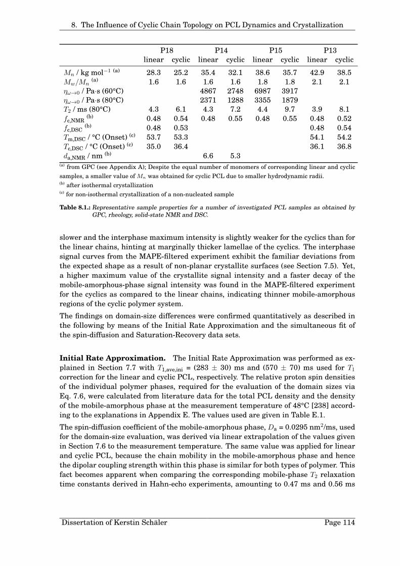
8. The Influence of Cyclic Chain Topology on PCL Dynamics and Crystallization
P18 P14 P15 P13linear cyclic linear cyclic linear cyclic linear cyclic
Mn / kg mol−1 (a) 28.3 25.2 35.4 32.1 38.6 35.7 42.9 38.5Mw/Mn
(a) 1.6 1.6 1.6 1.6 1.8 1.8 2.1 2.1ηω→0 / Pa·s (60°C) 4867 2748 6987 3917ηω→0 / Pa·s (80°C) 2371 1288 3355 1879T2 / ms (80°C) 4.3 6.1 4.3 7.2 4.4 9.7 3.9 8.1fc,NMR
(b) 0.48 0.54 0.48 0.55 0.48 0.55 0.48 0.52fc,DSC
(b) 0.48 0.53 0.48 0.54Tm,DSC / °C (Onset) (c) 53.7 53.3 54.1 54.2Tc,DSC / °C (Onset) (c) 35.0 36.4 36.1 36.8da,NMR / nm (b) 6.6 5.3
(a) from GPC (see Appendix A); Despite the equal number of monomers of corresponding linear and cyclicsamples, a smaller value of Mn was obtained for cyclic PCL due to smaller hydrodynamic radii.(b) after isothermal crystallization(c) for non-isothermal crystallization of a non-nucleated sample
Table 8.1.: Representative sample properties for a number of investigated PCL samples as obtained byGPC, rheology, solid-state NMR and DSC.
slower and the interphase maximum intensity is slightly weaker for the cyclics than forthe linear chains, hinting at marginally thicker lamellae of the cyclics. The interphasesignal curves from the MAPE-filtered experiment exhibit the familiar deviations fromthe expected shape as a result of non-planar crystallite surfaces (see Section 7.5). Yet,a higher maximum value of the crystallite signal intensity and a faster decay of themobile-amorphous-phase signal intensity was found in the MAPE-filtered experimentfor the cyclics as compared to the linear chains, indicating thinner mobile-amorphousregions of the cyclic polymer system.
The findings on domain-size differences were confirmed quantitatively as described inthe following by means of the Initial Rate Approximation and the simultaneous fit ofthe spin-diffusion and Saturation-Recovery data sets.
Initial Rate Approximation. The Initial Rate Approximation was performed as ex-plained in Section 7.7 with T1,ave,ini = (283 ± 30) ms and (570 ± 70) ms used for T1correction for the linear and cyclic PCL, respectively. The relative proton spin densitiesof the individual polymer phases, required for the evaluation of the domain sizes viaEq. 7.6, were calculated from literature data for the total PCL density and the densityof the mobile-amorphous phase at the measurement temperature of 48°C [238] accord-ing to the explanations in Appendix E. The values used are given in Table E.1.
The spin-diffusion coefficient of the mobile-amorphous phase, Da = 0.0295 nm2/ms, usedfor the domain-size evaluation, was derived via linear extrapolation of the values givenin Section 7.6 to the measurement temperature. The same value was applied for linearand cyclic PCL, because the chain mobility in the mobile-amorphous phase and hencethe dipolar coupling strength within this phase is similar for both types of polymer. Thisfact becomes apparent when comparing the corresponding mobile-phase T2 relaxationtime constants derived in Hahn-echo experiments, amounting to 0.47 ms and 0.56 ms
Dissertation of Kerstin Schäler Page 114

8. The Influence of Cyclic Chain Topology on PCL Dynamics and Crystallization
(a) (b)
Figure 8.9.: Spin-diffusion curves for linear and corresponding cyclic PCL (Mn,lin = 35.4 kg/mol) measuredat 48°C after isothermal crystallization at 48°C for 4 days in DQ-filtered (a) and MAPE-filtered (b) spin-diffusion experiments.
for the linear and cyclic PCL, respectively. According to the calibration of the mobile-phase spin-diffusion coefficient as a function of the T2 time constant given by Mellingeret al. [129,251] the difference between the T2 values for linear and cyclic chains resultsin a difference of the corresponding spin-diffusion coefficents of 4.5%. Such a smalldeviation ranges within the uncertainty margin (∼10%) of the coefficients determinedin Section 7.6.
The rigid-phase spin-diffusion coefficient, Drig = 0.31 nm2/ms, was calculated as a weigh-ted mean from the coefficients of the crystalline phase and interphase given in Sec-tion 7.6 according to Eq. 7.5. Again, the same value was used for linear and cyclic PCL,based on the assumption of very similar average coupling strengths in the crystallitesdue to a similar crystallite structure, which is indicated by the very similar second mo-ments M2 of the proton line shapes, ranging at about 10400 kHz2 for linear and cyclicPCL over the whole range of molecular weights investigated here.7 The similarity ofthe crystallite structure of linear and cyclic PCL of high molecular weight was in factconfirmed by Shin et al. on the basis of WAXS measurements [297].
According to the findings in Section 7.7 the IRA analysis was performed for the crystal-line-phase-selected (DQ-filtered) spin-diffusion experiment using Eq. 7.6. The resultsare listed in Table 8.2. As supposed above after comparing the spin-diffusion curvesqualitatively, the cylic PCL chains formed thinner mobile-amorphous domains comparedto their linear analogues. The size difference amounts to about 1 nm. Yet, no differencewas detected for the interphase and crystalline-phase domain thicknesses of the linearand cyclic PCL within the uncertainty ranges.
Simultaneous Fit of Spin-Diffusion and Saturation-Recovery Data. More pre-cise domain-size results were obtained from simultaneous fits of the crystalline-phase-selected (DQ-filtered) spin-diffusion curves and the Saturation-Recovery data as de-scribed in Sections 7.3 and 7.6. The starting values for the spin-diffusion coefficents in
7M2 was calculated from the parameters a and b from fits to the MSE signals via Eq. 4.3 (see Section 4.1).
Dissertation of Kerstin Schäler Page 115

8. The Influence of Cyclic Chain Topology on PCL Dynamics and Crystallization
√t0 /√
ms da /nm drig /nm dc /nm di /nm
linear 33.8 ± 1.0 6.6 ± 0.3 9.7 ± 0.4 7.79 ± 0.96 0.96 ± 0.23cyclic 35.6 ± 1.0 5.5 ± 0.2 10.2 ± 0.4 8.25 ± 0.98 0.97 ± 0.23
Table 8.2.: Results from the Initial Rate Approximation for spin-diffusion data of linear and cyclic PCL(Mn,lin = 35.4 kg/mol) at 48°C
the fit were chosen to be Da = 0.0295 nm2/ms, Di = 0.19 nm2/ms and Dc = 0.34 nm2/msaccording to the findings in Section 7.6, and the initial T1 parameter values were setto the apparent T1,ini time constants of the individual phases, obtained from linear fitsto the initial rises of the corresponding Saturation-Recovery curves (see Section 5.1).For the domain thicknesses the results from the IRA analysis (see above) were selectedas starting values. In order to obtain reliable domain thicknesses, in the fits the spin-diffusion coefficients were kept fixed at the starting values, leaving the thicknesses andT1 time constants as free fit parameters.8 Fit parameters have been reset, if physicallyunreasonable combinations of the parameter values arose, such as Di > Dc or T1i > T1c(see Appendix F.4). Moreover, in order to define an uncertainty level of the thicknessresults obtained from the fit, the starting values of the spin-diffusion coefficients werevaried within the uncertainty ranges given in Section 7.6. Despite partially noisy datathe fitting quality was good. A comparison between the measured data and the fit curvesis depicted exemplarily in Fig. 8.10 and the results for the fit parameters are given inTable 8.3.
(a) (b)
Figure 8.10.: Simultaneous fit to DQ-filtered spin-diffusion and Saturation-Recovery data, measured at48°C for linear and corresponding cyclic PCL (Mn,lin = 35.4 kg/mol): (a) spin-diffusion curvesfor the DQ-filtered experiment, (b) Saturation-Recovery curves. The solid and dashed linesrepresent the fit curves. Results for the fit parameters are summarized in Table 8.3.
Within the uncertainty margins, the domain thicknesses found here are in good agree-ment with the results from the IRA analysis (see above), confirming that the mobile-amorphous domains were smaller for the cyclic PCL as compared to the linear analogueby about 1.3 nm. This thickness difference corresponds to the length of about 1.5 PCL
8Only at the end of the fitting procedure, the diffusion coefficient values were allowed to adjust freely (atfixed thicknesses) to ensure a further approach to the fit minimum. Yet, the resulting values hardlydeviated from the initial values.
Dissertation of Kerstin Schäler Page 116

8. The Influence of Cyclic Chain Topology on PCL Dynamics and Crystallization
repeat units. According to the results from the simultaneous fits of spin-diffusion andSaturation-Recovery data, moreover, the crystal thickness of the cyclics is slightly larger(by about 0.3 nm) than found for the linear PCL. Consequently, as the interphase do-main sizes do not show any topology effect, the long period is somewhat smaller (byabout 0.8 nm) for the cyclics in comparison to the linear analogue. The latter finding isin contrast to the results of Shin et al. who reported equal crystal thicknesses and longperiods of linear and cyclic PCL obtained from SAXS experiments, however, withoutstating concrete numbers [297].
mobile-amorphous rigid-amorphous crystalline totalphase interphase phase
linear
d / nm 6.57±0.09 0.95±0.03 7.77±0.11 16.24±0.26D / nm2 ms−1 0.0293±0.0004 0.22±0.05 0.38±0.07T1 / ms 115±1 130±10 550±35
cyclic
d / nm 5.28±0.08 0.97±0.03 8.13±0.09 15.35±0.23D / nm2 ms−1 0.0293±0.0004 0.19±0.03 0.37±0.05T1 / ms 107±6 120±10 760±120
Table 8.3.: Domain thicknesses d, spin-diffusion coefficients D, longitudinal relaxation time constantsT1 and long period L (last column) as obtained from simultaneous fits of spin-diffusion andSaturation-Recovery data for linear and cyclic PCL (Mn,lin = 35.4 kg/mol) at 48°C (see text).The uncertainties represent the ranges of fluctuation of the fitting results for slighly differentstarting parameters.
8.4. Summarizing Remarks
The comparison of PCL chains of linear and cyclic topology yielded the following overallpicture (see Fig. 8.11):
• 1H low-field NMR Hahn-echo and multiple-quantum measurements revealed alower residual order of the chain segments and a faster loss of orientational mem-ory in the melt of rings when compared to the linear analogues, resulting from lessor weaker topological restrictions to chain motion, such as entanglements and/orpacking constraints. The enhanced cyclic-chain mobility was also reflected in thelower melt viscosities of the cyclic polymers in comparison to their linear counter-parts.
• The higher chain mobility in the melt enabled an easier, i. e. faster crystal growthof the cyclics in comparison to the linear chains, resulting in a higher crystallinityas observed by means of DSC and 1H low-field NMR MSE measurements dur-ing non-isothermal and after isothermal crystallization. Large effects of missingchain ends of the cyclics on the fold-surface energy of the crystals and on the crys-tallization process can be excluded, as for the high molecular weights used herethe chain-end concentration in the fold surface (roughly estimated for an adjacent-reentry scenario and a crystal thickness of 8 nm) does not exceed 6%.
Dissertation of Kerstin Schäler Page 117

8. The Influence of Cyclic Chain Topology on PCL Dynamics and Crystallization
• From the results of the spin-diffusion measurements one can conclude, that thehigher crystallinity of the cyclic PCL is based on a reduced size of the mobile-amorphous domains compared to the linear polymer, while the crystal thicknessis increased only marginally. This finding is consistent with the lower number ofpacking restrictions for cyclic chains in the melt, which counteract the crystalliza-tion, hence allowing the formation of thinner mobile-amorphous regions.
Figure 8.11.: Schematic representation of the semicrystalline structure of linear and cyclic PCL form-ing from the coiled melt state.
Dissertation of Kerstin Schäler Page 118

9. Summary
9. Summary
Proton low-field NMR methods are well-suited for investigations of the phase structureof semicrystalline polymers and the chain dynamics within their crystalline and mobile-amorphous regions. The main issue here is the sensitivity of the NMR time-domainsignal to the strength of the homonuclear dipolar couplings between the protons in thesample. The reduction of this coupling strength as a result of molecular motions and dif-ferences between the coupling strengths in the individual polymer phases are observeddue to their characteristic effect on the signal shape and intensity. Both influences havebeen exploited in this thesis in order to study the semicrystalline polymers PCL and PE.
Crystallinity and Crystal-Growth Investigations. Based on mobility distinctionsor rather differences in the anisotropy of fast chain motions between amorphous andcrystalline polymer phases, the crystallinity of PCL and PE could be determined reliablyby means of FID measurements at temperatures far above the glass transition. Thecrystallinities obtained by low-field NMR are comparable to values from SAXS and DSCmeasurements. Since a model fit function has been adapted for a stable fit of the NMRtime-domain signals, a fast analysis of the phase composition of the samples is possible.For both polymers, PCL and PE, besides the crystalline-phase and mobile-amorphous-phase signal a third contribution had to be introduced in order to attain a high fittingquality. This contribution is ascribed to the signal of a rigid-amorphous interphase ofrestricted chain mobility between crystallites and mobile-amorphous regions.
The isothermal crystallization of PCL could be tracked reproducibly by NMR FID (orMSE) measurements. As PCL exhibits a self-seeding or melt-memory phenomenon, thesamples had to be molten at a sufficiently high temperature (above ∼85°C) in order toprevent unpredictable effects of surviving self nuclei on the kinetics of a subsequentcrystallization. Also impurities influence the crystallization kinetics by acceleratingthe nucleation step. The crystal-growth rate of different samples is comparable onlyif they exhibit a similar, high number of external nuclei. Hence, it is recommendableto blend PCL samples with chloro-substituted DBS as a nucleating agent to eliminatethe nucleation as the rate-determining step of the crystallization process, when crystal-growth kinetics shall be compared.
Investigations of Dynamics in PE and PCL crystallites. The MSE sequence hasan advantage over the FID in that it prevents signal loss during the receiver dead time.When using the MSE for crystallinity determinations, however, phase-specific intensitycorrections have to be considered to compensate for the loss due to strong dipolar cou-plings and technical imperfections of the sequence or molecular dynamics on an inter-mediate time scale of microseconds to milliseconds. Yet, the systematic signal loss dueto such motions enables the application of the MSE sequence to study polymer dynamicswithin the crystallites.
Here, the MSE sequence was used to explore the time scale of the local 180° helicaljumps in PE crystallites. The investigation of this jump process by NMR is difficultas many NMR interactions, such as the geminal proton dipolar couplings, the chemicalshifts and 2H quadrupolar interactions are invariant under the flip motion. However, asshown here, one can exploit the fact that the strength of the dipolar couplings between
Dissertation of Kerstin Schäler Page 119

9. Summary
protons of a moving chain and protons of the neighboring chains is changed compared tothe static case, leading to a systematic reduction of the MSE refocusing efficiency, whenchain flips take place on the time scale of the sequence length. Jump rates for the localchain-flip process have been determined quantitatively for three PE samples of differentmolecular weight and lamellar thickness and different forms of the crystallite chain-foldsurface (tight chain folds vs. disordered fold surface). For this purpose, FID signal de-composition has been used and the Anderson-Weiss approach to describe the MSE crys-tallite signal intensity decay as a function of the MSE sequence length. The jump ratesobserved here agree well with results from advanced, complex and time-consuming 13C-based high-field NMR experiments. Within the available time and temperature windowof the method the differences in phase morphology as well as in molecular weight andlamellar thickness did not influence the chain-flip rate significantly, although a consider-able difference in the speed of the longer-range chain transport through the crystalliteswas reported in literature for samples similar to the ones investigated here. Appar-ently, this difference is not based on different jump rates of the local flip process. Yet,for the reactor powder samples, exhibiting an adjacent-reentry-like morphology, slightlysmaller activation energies were found than for melt-crystallized PE with its disorderedfold surfaces.
Following the interpretation of Kaji and Horii the methylene groups in the PCL crystal-lites should perform rather large-amplitude motions (up to 90°) on an intermediate toslow time scale. However, neither the results of low-field MSE measurements nor thesecond moment M2 of the proton line shape as a function of temperature give any hintsto intermediate motions within the PCL crystallites. Moreover, findings from high-fieldNMR DIPSHIFT and CODEX experiments, performed to check the low-field results andto extend the available time scale for the observation of motions, confirmed the absenceof intermediate-regime and slow motions. Only fast motions, presumably vibrations,with amplitudes up to about 20° have been proven by means of the DIPSHIFT method.Since jump motions of large amplitudes are not present within the PCL crystallites,chain diffusion through the crystallites and crystal thickening during crystallization orcooling as known for PE are not expected for PCL. The absence of crystal thickeningprocesses was in fact confirmed by SAXS measurements. Hence, a classification of PCLas a crystal-fixed polymer is justified.
Investigations of the Domain Morphology in PCL by Means of Spin-DiffusionExperiments. As shown here exemplarily for PCL, spin-diffusion experiments enablethe determination of domain sizes in semicrystalline polymers provided that the spin-diffusion coefficients are known. This method again relies on the differentiation of theindividual polymer phases on the basis of different chain mobility and dipolar couplingstrengths. It is favorable compared to other techniques as no particular sample pre-treatment is required, such as staining or degassing.
The selection of magnetization in one of the PCL phases has been accomplished bymeans of the MAPE sequence as a mobile-phase filter and a short DQ filter as a crys-talline-phase filter. The filter length of both sequences has been optimized for the ap-plication to PCL. However, a perfect excitation of magnetization in only one polymerphase has not been possible due to mobility gradients within the amorphous phase anda lack in filter efficiency of the DQ filter. Using the DQ filter, moreover, it was found
Dissertation of Kerstin Schäler Page 120

9. Summary
that the magnetization level within the crystalline lamellae after the application of thefilter was not equal for all the lamellar stacks as a result of the orientation dependenceof the dipolar couplings mediating the filter action and the different orientations of thestacks of lamellae. As opposed to glassy-amorphous polymer systems this uneven mag-netization distribution could not be equilibrated at short times, because of the missingcontact between the lamellar stacks of different orientations.
The spin-diffusion curves of PCL exhibit specific deviations from curves, which havebeen simulated under the assumption of one-dimensional spin diffusion via planar in-terfaces in a system comprising two or three polymer phases, taking into account phase-specific T1 relaxation. The delayed magnetization transfer compared to the simulationcould be explained quantitatively by the existence of lag phases which are evaluated as apart of the magnetization source region but in fact are unpolarized initially. The directlytraceable reasons for magnetization transfer lags (i. e. the incomplete polarization of theindividual source phases by the filter sequences) do not suffice quantitatively to explainthe deviation from the simulated curves. The remaining difference, in particular thetoo low interphase signal intensity and the too high crystalline-phase signal intensityin the MAPE-filtered spin-diffusion curves, probably arise from corrugated crystallitesurfaces causing an enhanced magnetization transfer from the mobile-amorphous do-mains to the crystallites compared to a scenario with planar crystallite surfaces. As thevariations between measured curves from the MAPE-filtered experiment and simulatedcurves were dramatic, it is strongly recommended to restrict the analysis to data fromDQ-filtered spin-diffusion experiments.
For the individual polymer phases in semicrystalline PCL neither calculated nor exper-imentally derived values for the spin-diffusion coefficients have been reported in litera-ture up to now. However, these values are required for the estimation of domain sizesby means of NMR spin-diffusion experiments. Hence, they have been determined hereby fitting measured DQ-filtered spin-diffusion and Saturation-Recovery curves with thehelp of simulated curves, calculated for one-dimensional spin diffusion via planar sur-face boundaries in a three-phase polymer system with fixed domain thicknesses derivedfrom SAXS measurements. This way, effective spin-diffusion coefficients were obtainedfor all three PCL phases for temperatures of about 27°C to 45°C. Using these coeffi-cients, the domain sizes derived by SAXS could be reproduced well by means of theInitial Rate Approximation (IRA) of the DQ-filtered spin-diffusion data, confirming thepracticability of the IRA approach.
Influence of Chain Topology on the Semicrystalline Structure of PCL. A vari-ety of low-field NMR techniques complemented by rheological investigations and DSCstudies have been applied to linear and macrocyclic PCL chains of the same chain lengthin order to compare their mobility in the melt, their crystal-growth kinetics and theirsemicrystalline structure. The melt of PCL rings exhibited a higher chain mobility com-pared to the linear chains, observed in the form of a lower residual order and a fasterloss of orientational memory of the chain segments as a result of less or weaker topologi-cal restrictions to chain motion, such as entanglements and/or packing constraints. Dueto the enhanced mobility the cyclics crystallized faster and finally reached a higher crys-tallinity in comparison to the corresponding linear chains. As proven by spin-diffusionmeasurements using the spin-diffusion coefficients derived for PCL before, this gain in
Dissertation of Kerstin Schäler Page 121

9. Summary
crystallinity is not caused by thicker lamellae but by thinner mobile-amorphous regionsof the cyclic PCL essentially because, compared to the linear chains, less packing con-straints counteracted the crystallization.
Dissertation of Kerstin Schäler Page 122

A. Experimental Details
A. Experimental Details
A.1. Experimental Techniques
1H Low-Field NMR. The 1H low-field time-domain measurements were carried outon Bruker minispec mq20 spectrometers with a static magnetic field of about 0.5 Tand 1H Larmor frequencies of 19.9 MHz to 20.0 MHz, equipped with commercial widetemperature range static probes. The spectrometers featured 90° pulse lengths of 1.6 µsto 3.0 µs and receiver dead times of 11 µs to 15 µs.
For the NMR measurements about 0.3 g of sample were packed into 8 mm or 10 mmNMR sample tubes in form of small pieces. The tubes were flame-sealed under vacuumconditions if necessary in order to avoid degradation of the samples (see Appendix B). Tokeep the sample in the center of the magnet, i. e. in the region of the highest homogene-ity of the magnetic field, only the lowermost 6 mm to 8 mm of the tubes were filled withsample. The sample tubes were centered in the middle of the spectrometer coil regionby custom-made Teflon spacers.
The sample temperature was regulated by means of a BVT3000 heater with air as theheat-transfer medium for heating and cooling. A cooler was required for temperaturesbelow 300 K. At temperatures below 230 K nitrogen gas was used as a cooling gas in-stead of air to prevent the condensation and freezing of water (air moisture) inside thecooling hoses. The temperature at the sample position could be set with an uncertaintyof about 1 K and a temperature gradient over the sample of 0.5 K. Temperature mea-surements at the sample position inside the spectrometer have been accomplished bymeans of an external thermo sensor which was put into a NMR sample tube, filled witha small amount of silicone oil, and placed at the sample position. The temperature atthe sample position was checked after each change of the temperature setting of theheater and also regularly between measurements at the same temperature setting.
All time-domain NMR signals were recorded on-resonant and in full-absorption modereceiver setting, analyzing only the real part of the complex time-domain signal. Asetup was made in the beginning of a series of measurements for every sample (yet,at least once a day) comprising a nutation experiment for the determination of the 90°and 180° pulse length. Moreover, to ensure that the longitudinal relaxation was com-plete between the scans in the semicrystalline state of the sample as well as in themelt, an appropriate recycle delay was determined either by variation of this delay orby means of a Saturation-Recovery experiment. For semicrystalline PCL and PE therecycle delay was typically set to 1.5 s and 2 s to 4.8 s, respectively. (Note, that forthe Saturation-Recovery measurements a very short delay of 0.1 s was sufficient, be-cause the magnetization was destroyed again before every new scan.) The number ofscans was varied between 16 and 512 depending on the NMR sequence used, in order toensure a sufficiently high signal-to-noise ratio.
High-Field 13C NMR DIPSHIFT Sequence. The DIPSHIFT sequence used is shownin Fig. A.1 adopted from Ref. [173]. A short description of its mode of operation is givenin the following. The sequence is performed under Magic-Angle Spinning (MAS) of thesample in order to enable the acquisition of high-resolution 13C spectra. Transverse13C magnetization is excited by means of Cross Polarization (CP). Subsequently, the
Dissertation of Kerstin Schäler Page 123

A. Experimental Details
spin system develops under the influence of resonance offsets and 1H-13C heteronucleardipolar couplings during an incremented time t1, which is varied between 0 and a fullrotor period TR (see Fig. A.1). During this time the homonuclear proton dipolar couplingis suppressed by means of the frequency-switched Lee-Goldberg (FSLG) decoupling se-quence [170,173]. For the rest of the sequence the system develops under heteronucleardecoupling using the SPINAL64 sequence [173]. The 180° pulse on the 13C channel aftera complete rotor period TR serves to generate a Hahn echo at the beginning of the signalacquisition period after 2TR, i. e. it cancels resonance offsets. Hence, effectively, theheteronuclear dipolar coupling is the only NMR interaction which influences the spinsystem during t1 and contributes to the detected signal [170].
The signal intensity varies with increasing t1 in a way which is characteristic for thestrength of the average 1H-13C coupling. Therefore this coupling strength can be de-rived here [170, 173]. It may be reduced by a pre-averaging of the couplings due tofast molecular motions with rates much larger than the static coupling strength and itsactual value yields information about the presence of fast motions and their motionalamplitude provided that the geometry of the motion is known.
Figure A.1.: Schematic sketch of theDIPSHIFT pulse sequence.The abbreviation SL desig-nates a spin lock for CrossPolarization (CP).
The DIPSHIFT experiments were performed on a Bruker Avance III spectrometer withan Oxford magnet, at 1H and 13C Larmor frequencies of 400.16 MHz and 100.06 MHz,respectively, equipped with a 4 mm double-resonance probe at a spinning frequencyof 5 kHz. The PCL sample was packed into a 4 mm ZrO2 MAS rotor. The tempera-ture accuracy was ±1 K. The 90° pulse lengths were 3.5 µs for 1H and 3.1 µs (at roomtemperature) or 3.0 µs (at 52°C) for 13C, respectively. For heteronuclear decoupling theSPINAL64 sequence was applied at a 1H decoupling frequency of 71.5 kHz. For homonu-clear decoupling with FSLG an rf field strength ωeff = 87.5 kHz along the effective fieldwas used. The contact time for 1H-13C Cross Polarization was chosen to be 0.3 ms andthe repetition delay was set to 2 s. 2048 scans were acquired for each of the 16 t1 incre-ments.
High-Field 13C NMR CODEX Sequence. The CODEX sequence used is shown inFig. A.2 adopted from Ref. [173]. Its mode of operation is shortly described in the follow-ing. Transverse 13C magnetization is excited using Cross Polarization (CP). After that,during N/2 rotor periods (with N being an integer), the spin system develops under theChemical-Shift Anisotropy (CSA) interaction, which is reintroduced by means of a seriesof rotor-synchronized 180° pulses applied every half a rotor period (see Fig. A.2) [190]. A90° store pulse serves to store magnetization in the direction of the magnetic field dur-
Dissertation of Kerstin Schäler Page 124

A. Experimental Details
ing the mixing time τmix < T1, being an integer multiple of the rotor period TR. Duringthis mixing time the magnetization does not precess or dephase but it develops underthe influence of slow molecular dynamics, if present in the sample [190, 191]. Subse-quently, the magnetization is flipped into the transverse plane by means of another 90°pulse and develops again under the reintroduced CSA interaction during N/2 rotor pe-riods [190]. The sequence is completed by storage of the magnetization in direction ofthe magnetic field during a short time tz = TR and the acquisition of the exchange signalafter a read-out pulse.
Figure A.2.: Schematic sketch of the CODEX pulse sequence. The abbreviation SL designates a spinlock for Cross Polarization (CP).
When slow segmental reorientations occur during τmix, i. e. on a time scale of millisec-onds to seconds, which change the orientation-dependent CSA interaction of the carbonspins, a dephasing of magnetization takes place, which is not reversed until the be-ginning of the signal acquisition period and is detected in the form of an intensity losscompared to a situation without molecular motions. The signal intensity as a function ofthe mixing time τmix or the duration NTR of the CSA recoupling periods yields informa-tion about the correlation time and amplitude of slow motions, respectively [190, 191].For the latter the geometry of the motion has to be known.
In order to cancel T1 relaxation effects during τmix and T2 relaxation effects during theCSA recoupling periods, a reference signal is detected using the same sequence butwith interchanged durations of τmix and tz. Here, τmix = TR is short, preventing slowdynamics during the mixing time. For normalization the exchange signal intensity isdivided by this reference signal intensity [191].
The CODEX experiments were performed on a Bruker Avance II spectrometer with aJastec magnet at 1H and 13C Larmor frequencies of 400.16 MHz and 100.06 MHz witha 4 mm double-resonance MAS probe at a spinning frequency of 5 kHz. The sample waspacked into a 4 mm ZrO2 MAS rotor and the temperature accuracy amounted to ±1 K.The 1H and 13C 90° pulse lengths were 3.0 µs and 3.7 µs, respectively. The SPINAL64sequence was applied for heteronuclear 1H-13C decoupling during the recoupling andacquisition period with a decoupling frequency of 80 kHz. For 1H-13C Cross Polarizationthe contact time was set to either 0.2 ms or 1.5 ms. The repetition delay was chosen tobe 2 s. Exchange and reference spectra were measured for CSA recoupling durationsNTR between 0.4 ms and 3.2 ms with 1024 scans each and a mixing time τmix of either100 ms or 200 ms.
Dissertation of Kerstin Schäler Page 125

A. Experimental Details
Small Angle X-Ray Scattering (SAXS). The Small Angle X-Ray Scattering (SAXS)measurements and data analysis were done by M. Sc. A. Seidlitz at the Institute ofPhysics (Experimental Polymer Physics group) of the Martin-Luther-Universität Hallewith a PCL sample analogous to the one used for the low-field NMR spin-diffusion ex-periments described in Section 7.2.
The SAXS apparatus contained a Cu-Kα X-ray source (wave length λ = 0.154 nm) witha beam focus of 0.4×12 mm2, refocusing X-ray lenses and a Kratky camera includingthe collimator system. The detection was carried out by means of a scintillation counterplaced in a distance of 200 mm from the temperature-controlled sample holder [218].
The SAXS measurements were performed under the same temperature conditions asfor the corresponding low-field NMR spin-diffusion and Saturation-Recovery measure-ments (cf. Section 7.2). For this purpose, the temperature setting of the NMR spectrom-eter and the SAXS sample holder was adjusted prior to the measurements by comparingthe readout of one temperature sensor in both devices.
The scattering intensities measured by SAXS were deconvoluted using a desmearingalgorithm to consider the line-shaped beam focus. The SAXS signal amplitude is propor-tional to the three-dimensional Fourier transform of the electron density in the sample.In case of a lamellar system it can be traced back to a one-dimensional electron densitycorrelation function, the second derivative of which is the interface distance distribu-tion function [218,312]. Such distribution functions were calculated from the measureddata and fitted by means of a simulated function which comprises the thicknesses ofthe crystalline and amorphous domains and the corresponding distribution widths asfit parameters. The fit enabled the determination of domain sizes also at crystallinitiesclose to 50% [218].
Differential Scanning Calorimetry (DSC). Differential Scanning Calorimetry wascarried out by means of a Perkin Elmer DSC7 and a Perkin Elmer Pyris Diamond instru-ment calibrated with indium and mercury and indium and cyclopentane, respectively.The measurements were conducted by K. Herfurt in the Experimental Polymer Physicsgroup at the Institute of Physics of the Martin-Luther-Universität Halle. Samples of5 mg to 10 mg were encapsulated in pressure-tight 30µl or 50µl aluminum pans. Ni-trogen was used as purge gas. The data were analyized by means of the software PyrisThermal Analysis version 3.81 or version 5.00.02 including a baseline subtraction for allnon-isothermally measured DSC curves.
For evaluating the crystallinity after isothermal crystallization, each sample was pre-treated non-isothermally by keeping it in the melt at 90°C for 10 minutes, cooling to 0°Cat -10 K/min, holding at 0°C for 10 minutes and re-heating to 90°C. After 10 minutes inthe melt the sample was rapidly cooled to the crystallization temperature (at -200 K/minor the highest possible cooling rate) and isothermally crystallized for a crystallizationtime tc. From the subsequent heating scan to 90°C at 10 K/min heat flow and enthalpyof fusion were determined for the estimation of the crystallinity. Moreover, as a checkfor consistency, the pretreatment steps were repeated.
In order to investigate the non-isothermal crystallization, the melting and crystalliza-tion temperatures (evaluated at the peak onsets) were deduced from heat-flow curvesobtained during heating to 100°C (after cooling from the melt (at 100°C) to 0°C and hold-
Dissertation of Kerstin Schäler Page 126

A. Experimental Details
ing the sample at 0°C for 10 minutes) and a second cooling run to 0°C after annealing at100°C for 10 minutes. All cooling and heating steps were conducted at 10 K/min.
The glass transition temperatures of the amorphous regions of the semicrystalline PCLsamples were measured upon heating to 85°C at 20 K/min after having cooled the sam-ple from the melt to -100°C at 20 K/min and annealing for more than 10 minutes. Theglass transition was visible and the glass transition temperatures Tg were determinedas the midpoints of the glass transition step. The Tg values did not differ by more than1 K to 2 K. Within the scatter no significant trend concerning a differentiation betweenlinear and cyclic PCL was observed. Hence, also at higher temperatures (i. e. in themelt) significant deviations of the segmental dynamics between linear and cyclic chainscaused by free volume differences are not expected.
Gel Permeation Chromatography (GPC). Gel Permeation Chromatography (GPC)measurements were performed by a staff member of the Division of Macromolecular Sci-ence in the Department of Macromolecular Chemistry at the Martin-Luther-UniversitätHalle at a Viscotek GPCmax VE 2001 apparatus with a Styragel linear column GMHHRwith tetrahydrofuran (THF) as a carrier solvent at 1 ml/min at room temperature. Thesample concentration was approximately 3 mg/ml.
Polystyrene standards (Mp = 1050 - 115000 g/mol) were used for conventional exter-nal calibration, using a Waters RI 3580 refractive index detector. The absolute PCLmolecular weights were calculated from the apparent ones (for PS standard) usingthe Mark-Houwink equation [313] and the parameters or formulas given in the liter-ature [314–317].
Rheological Measurements. Rheological measurements were performed by Dr. K.Schröter and Dipl.-Chem. E. Ostas at the Institute of Physics (Experimental PolymerPhysics group) of the Martin-Luther-Universität Halle, using a Rheometrics DynamicAnalyzer RDAII with a parallel-plate geometry purchased from TA Instruments. Thediameter and the thickness of the samples were 25 mm and around 1.7 mm, respectively.In this case, compliance effects of the instrument are negligible. Shear loss modulus(G′′) and storage modulus (G′) were determined as a function of the shear frequencyω between 1 rad/s and 100 rad/s. Typically, the strain in the sample was 2%, being wellwithin the linear deformation range. The strain was chosen to keep the measured torquevalues in a range of about 100 g·cm to 0.2 g·cm, according to the measurement range ofthe transducer of the instrument. At low frequencies the decreasing modulus values andhence also the torque values limited the usable measurement range of the rheometer.
For sample preparation the PCL powder was pressed under vacuum in a cylindricalmould with the desired diameter and thickness. After 8 h at 90°C the sample was slowlycooled down to room temperature over night under vacuum. The cylindrical polymersample was placed between the two plates of the rheometer and after heating to 90°Cand slight compression it stuck to the surface of the plates. Subsequently, the temper-ature was lowered to the measurement temperatures of 60°C or 80°C and equilibrated.During these temperature changes the thermal expansion of the tools of the instrumentwas compensated by a corresponding change of the gap setting. Due to the air andhumidity sensitivity of cyclic PCL (see Appendix B) all measurements were conducted
Dissertation of Kerstin Schäler Page 127

A. Experimental Details
Figure A.3.: Synthetic approach for the preparation of cyclic and linear PCL (graph adapted fromRef. [242]).
under a nitrogen gas flow.
A.2. Samples
PCL Samples. For this work two kinds of PCL systems have been used, i. e. indus-trially produced PCL on the one hand and linear and cylic PCL synthesized by Dipl.-Chem. E. Ostas (Macromolecular Chemistry Department, Division of MacromolecularScience, Martin-Luther-Universität Halle) on the laboratory scale on the other hand.
The industrially produced PCL withMn ≈ 42.5 kg/mol and PD ≈ 1.5 (Mw ≈ 63.8 kg/mol)was purchased from Sigma Aldrich.
The cyclic PCL samples were prepared by E. Ostas by insertion polymerization accord-ing to procedures reported by Kricheldorf et al. [301]. For the ring opening polymer-ization of ε-caprolactone an Sn-based cyclic initiator (2,2-dibutyl-1,2-dioxa-2-stannane)((1) in Fig. A.3) was used, which does not allow for the concatenation of rings. Thecorresponding linear polymers were obtained directly from the respective cyclic PCLsby cleavage of the Sn-O bond with 1,2-ethane-dithiol to yield bis-hydroxytelechelic PCL[318]. They exhibit the same number of monomers as their cyclic counterparts and arefree of tin. Details on the synthesis are given in Refs. [242] and [319].
A number of PCL samples was blended with chloro-substituted dibenzylidene sorbitol(1,3:2,4-di(4-Chlorobenzylidene) Sorbitol) (cl-DBS) synthesized by E. Ostas accordingto the instructions given in Ref. [233]. For the solution blending of the samples, PCL(98.5 wt%) and cl-DBS (1.5 wt%) were dissolved in heated butanone separately. Thesolutions were mixed and the mixture was dried afterwards in a rotary evaporator andunder high vacuum.
PE Samples. Two types of PE samples were compared in Section 5.2, a commercialhigh-density (HD) PE and two reactor powders of ultra-high molecular weight.
The commercial HD PE sample was provided by Basell Polyolefine GmbH. It exhibits aweight-averaged molecular weight Mw ≈ 349 kg/mol and a polydispersity PD ≈ 21.4 (asmeasured by GPC). It was crystallized from the melt and exhibits lamellar crystals withdisordered fold surfaces (see Fig. 5.10). Because of the high polydispersity the samplecontains short chains possibly forming tight folds at crystalline surfaces as well as long
Dissertation of Kerstin Schäler Page 128

A. Experimental Details
chains which may form entanglements in the amorphous regions. The mass and volumecrystallinity of the HD PE amounts to 59 % and 55.4 %, respectively, determined by DSCand Wide Angle X-Ray Scattering (WAXS), respectively. Results from SAXS revealed along period L ≈ 21 nm. The lamellar thickness dc ≈ 13 nm was estimated using thecrystallinity data. The melting temperature was quantified to be 405 K by DSC (heatingrate: 20 K/min).
The two PE reactor powder samples were provided by Prof. S. Rastogi (LoughboroughUniversity). Information about sample preparation and properties is given in Ref. [199].Both samples show a rather adjacent-reentry-like morphology (see Fig. 5.10) but differin molecular weight (Mw ≈ 5000 kg/mol and 750 kg/mol) and polydispersity (PD ≈ 3and 1.8, respectively), derived from rheology. The lamellar thickness of both samplesranges at about 8 nm as estimated by transmission electron microscopy (TEM) [320].
Dissertation of Kerstin Schäler Page 129

B. PCL Degradation Investigations
B. PCL Degradation Investigations
B.1. Degradation of Cyclic PCL Chains
For testing the degradation of the cyclic PCL chains resulting from the cleavage of theSn-O bonds, linear, tin-containing PCL samples were prepared by E. Ostas (Macro-molecular Chemistry Department, Division of Macromolecular Science, Martin-Luther-Universität Halle) by means of a dibutyl-tin-dimethoxide initiator ((2) in Fig. A.3) TheSn-O bond cleavage separates these chains into two parts of about half the molecularweight. Such a large change in molecular weight causes a significant effect on the GPCretention volume and can be detected more clearly than the small difference betweencyclic chains and their linear counterparts, formed by the Sn-O bond cleavage of thecyclics (see also Fig. 8.1).
Two samples of accordingly prepared linear chains, i. e. a test sample and a referencesample, were placed in sealed glass tubes. While the reference sample was kept underan atmosphere of argon, the test sample was studied under ambient conditions (mois-ture and oxygen). The degradation test was performed by E. Ostas by annealing bothsamples at 95°C for some hours and by monitoring the molecular weights in regulartime intervals by GPC.
Figure B.1.: GPC traces for a linear tin-containingPCL (Mn = 16.1 kg/mol, Mw/Mn
= 1.7) at 95°C at ambient conditions(moisture and oxygen) and under ar-gon atmosphere. The bottom traces(t = 0) reflect the sample state beforecleavage. The measurement timesduring the cleavage experiment aregiven in the plot (graph adopted fromRef. [242]).
As can be seen in Fig. B.1, heating under ambient conditions afforded the appearance ofa second peak at higher retention volume, i. e. lower molecular weight due to cleavageof the Sn-O-bonds. By contrast, the reference sample did not show a significant changein molecular weight and thus no cleavage reactions. Similar degradation results areknown for PCL rings synthesized by click chemistry [259]. According to these findingsall further measurements were conducted under exclusion of air and moisture. More-over the samples were stored under vacuum.
B.2. Degradation of Linear PCL Chains
As chain degradation results in a shortening of the chains and hence in an enhancementof the chain mobility and a reduction of the residual dipolar coupling strength, T2 Hahn-echo measurement probing the residual dipolar coupling strength qualitatively, can beapplied to detect degradation effects.
Here, the long-term stability of linear PCL chains was tracked for a period of somemonths by means of Hahn-echo decay measurements at 80°C performed for two indus-trially produced PCL samples (Mn = 42.5 kg/mol, without tin) stored under different
Dissertation of Kerstin Schäler Page 130

B. PCL Degradation Investigations
conditions. Between the measurements the test sample was stored in an evacuatedsample tube at 90°C under natural light, whereas the reference sample was stored atroom temperature, under vacuum and in a dark environment.
Figure B.2.: Long-term stability test for linear PCL. Hahn-echo decay curves measured at 80°C for 2industrially produced PCL samples (Mn = 42.5 kg/mol): a reference sample (left), storedunder vacuum at room temperature in a dark environment, and a test sample (right),stored in an evacuated sample tube at 90°C under natural light.
In Fig. B.2 the Hahn-echo decay curves detected after increasing storage periods aredepicted for both samples. The decay time of the reference sample did not change dur-ing the test period. Yet, the decay observed for the test sample slowed down signifi-cantly with increasing storage time as a result of reduced residual dipolar couplingsdue to more isotropic chain motions (cf. Section 8.1) of the shorter PCL chains formedby chain degradation. Hence, it may be concluded that PCL chains decompose during(long) annealing periods at high temperatures, presumably by the random cleavage ofester bonds [321]. This finding has to be considered with regard to sample treatmentwhen a specific molecular weight is required.
Dissertation of Kerstin Schäler Page 131

C. Quantum-Mechanical Basics of NMR
C. Quantum-Mechanical Basics of NMR
The quantum-mechanical state of a nuclear spin system is described by the wave func-tion |ψ(t)〉, which contains information about the position, speed and spin state of ev-ery particle of the system. The time development of the system is specified by theSchrödinger equation
d
dt|ψ(t)〉 = − i
~H|ψ(t)〉 ,
where H is the Hamiltonian, a Hermitian operator describing the orientation depen-dence of the interaction energies in the spin system [53]. The corresponding observableis the energy of the system. The energy eigenfunctions of the Hamiltonian are stationaryand orthonormal and the eigenvalues, i. e. the energy levels of the spin system, are realvalues. In the following only the nuclear spin states and the nuclear spin Hamiltonianare considered, assuming that the effects of the rapidly moving electrons are averagedto a mean value, which is stable in time and contributes only a constant portion to thenet Hamiltonian [53].
The spin operator and the Zeeman Hamiltonian [17,53,54]. The atomic nucleuscarries a magnetic dipole moment µ and a spin I. These observables are associatedwith their quantum-mechanical analogues, the Hermitian operators µ and I, which arerelated to each other via
µ = γI
as in the macroscopic representation. Both operators are vectors with carthesian coor-dinates µx, µy, µz and Ix, Iy, Iz, which are Hermitian, too.
The spin operator I, similarly to the orbital angular momentum operator, fulfills theeigenequations
I2|I,mI〉 = I(I + 1)|I,mI〉 andIz|I,mI〉 = mI |I,mI〉 ,
where, I2
= I2x + I2y + I2z . A detailed describtion of the orthonormal eigenfunctions|I,mI〉 is usually not necessary. From the eigenequations one can learn that the lengthof the spin vector and one of the components1 are quantized with the corresponding spinquantum numbers I and mI . The former can take half-integer numbers (although I=2seems not to occur in nature) and the latter runs from −I to I. The quantum number Iis often used to characterize a nucleus, e. g., I = 1/2 for so-called spin-1/2 nuclei. Note,that the functions |I,mI〉 are no eigenfunctions of the spin operator components Ix andIy.
The interaction of the nuclear magnetic dipole moments with a magnetic field of strengthB is described by the Zeeman Hamiltonian
H0 = −~ (µ ·B) = −~γ(I ·B
)NMR measurements are usually performed in a strong static magnetic field B0, theorientation of which is chosen to be in z direction of the carthesian coordinate system,
1Here, we chose the z component as it is usually done in literature.
Dissertation of Kerstin Schäler Page 132

C. Quantum-Mechanical Basics of NMR
so thatH0 = −γB0~Iz = −ω0~Iz .
As the Zeeman Hamiltonian is proportional to Iz, both operators share the same eigen-functions |I,mI〉, forming the so-called orthogonal Zeeman eigenbasis. The energy eigen-values of the Hamiltonian can be found from
H0|I,mI〉 = −γ~B0Iz|I,mI〉 = −γB0~mI |I,mI〉 = −ω0~mI |I,mI〉 = EI,m|I,mI〉 ,
adopting values EI,m = −~ω0mI . Here, we find a splitting of energy levels, the Zeemansplitting, according to the value of the quantum number mI . The energy gap betweenthe Zeeman energy levels amounts to ~ω0 ≈ h·20 MHz ≈ 1.3·10−26J, which is very smallcompared to the thermal energy at 25°C (∼ 4.1·10−21J).
A nucleus in the magnetic field does not have to be in an eigenstate of H0 and Iz. In gen-eral it adopts a normalized superposition state, i. e. a linear combination of eigenstates:
|ψ〉 =∑j
αj |Ij ,mI,j〉 ,
where the prefactors αj specify the actual spin state [53].
Measurements of the observable of a quantum-mechanical operator (e. g., the energy ofthe spin system) always yield an eigenvalue of the corresponding operator. However, itis not known a priori which of them, i. e. the observable is not well-defined. The resultof a measurement is governed by statistics and one can only calculate a probability tofind a certain eigenvalue, when the system is in the state |ψ〉. (This probability amountsto 100%, when |ψ〉 is the corresponding eigenstate.) Moreover, the mean result after ahigh number of measurements, i. e. the expectation value, can be derived. As super-position states are no eigenstates of Iz and H0 they do not have well-defined energies(and spin components in z direction) and cannot be depicted in an energy level diagram.Nevertheless they are real states [53].
The polarization axis of a spin denotes the direction in space, along which the spin iswell-defined, i. e. the direction of a spin operator component, for which the present spinstate is an eigenstate. This component is not necessarily a carthesian one, but a linearcombination of them. As every orientation in space is related to such a component ofI, possessing an arbitrary superposition state as an eigenstate, the polarization axiscan take every direction [53].2 This axis is the quantum-mechanical analogue of thedirection of the spin vector in the macroscopic representation and one can, e. g., show,that it precesses about B0 by solving the Schrödinger equation (see above) for a spinin a superposition state with the Zeeman Hamiltonian describing the interaction withB0 [53].
The Spin Density Operator and its Time Development. For the calculation ofmacroscopic properties of the spin system, one can in principle sum up the individualquantities of all spins in the system. However, this is cumbersome and often not possible
2The often used representation of the spin vector, rotating on the surface of a cone with fixed openingangle, is only a model to explain the quantization of the spin in a descriptive way. It does not reveal anyinformation about the orientation of the spin vector in the magnetic field [53].
Dissertation of Kerstin Schäler Page 133

C. Quantum-Mechanical Basics of NMR
at all. For this reason the spin density operator
% = 〈(|ψ〉〈ψ|)〉
was introduced, which describes the quantum-mechanical state of the whole system asa kind of average spin state and is based on the expectation values of the observables.Here, |ψ〉 is again the wave function of the spin system and the outer angle bracketsdenote the average over all members of the spin ensemble [53].
The mean contribution of each individual spin to the macroscopic observable A of anoperator A is equal to the expectation value
〈A〉 = Tr(%A)
. (C.1)
Thus, the macroscopic quantity can be evaluated from the corresponding quantum-mechanical operator and the operator % describing the spin system as a whole.
When writing the density operator in the matrix form, the diagonal elements representthe populations of the eigenstates of Iz and the off-diagonal elements are interpreted ascoherences between two eigenstates [53].
Every (superposition) spin state comprises certain fractions of the distinct eigenstates.The population of an eigenstate can be understood as the sum of the portions of thiseigenstate of all the spins in the system. Populations are positive, real numbers rangingbetween 0 and 1. Their sum is equal to 1 as a result of the normalization of the spinstates. In the macroscopic representation for spins 1/2 the populations are related tothe sum of all spin vector components in or opposed to the direction of the magneticfield. Hence, a difference of the eigenstate populations, as present in thermal equi-librium where the populations follow a Boltzmann distribution, results in macroscopiclongitudinal magnetization.
Coherences between two eigenstates |j〉 and |k〉 are complex numbers which charac-terize particular states of the spin system. They are specified by the coherence ordero = mI,j −mI,k, calculated from the quantum numbers of Iz. In the thermal equilibriumcoherences of order o ≥ 1 are not available. A coherence of order o = 1 is a state of thespin system, where a certain orientation of the spin polarization axes in the transverseplane is preferred, so that transverse magnetization exists. Higher order coherences,i. e. so called multi-quantum coherences, develop under spin interactions, e. g., in dipo-larly coupled systems. They are not directly detectable in the form of magnetization.One can imagine such coherences as a correlation of the orientations of spins within agroup of interacting spins [53]. In the spin density operator higher order coherencesare characterized by distinct products of spin operator components. As an example, theexpression 2Ix,j Iy,k identifies a sum of two coherences with o = 0 and o = 2, i. e. azero-quantum and a double-quantum coherence. It describes a situation of pairs ofinteracting spins j and k, where none of the partners tends to orient in a particulardirection, but where the orientation of both partners correlates with each other. Whenspin j points into +x direction, there is a high probability for spin k to be oriented in+y direction, but still the overall orientation of pairs of spins is isotropic, preventing thebuild-up of magnetization.
In the thermal equilibrium in the magnetic field and in case of high temperatures,
Dissertation of Kerstin Schäler Page 134

C. Quantum-Mechanical Basics of NMR
i. e. when |~γB0/kT | � 1 (which is the case for T � 1 K), the spin density operatoris given by
%eq ∼ (1/2)E + (1/2)IzE .
For practical purposes the unity operator E is usually skipped as it does not repre-sent detectable transverse magnetization. Also the prefactor is omitted, because it onlyvaries the signal amplitude, which is commonly not of interest. Thus, Iz is considered asthe equilibrium spin density operator. The measured signal is calculated using Eq. C.1.As an example, for the measured transverse magnetization after a 90° pulse we obtain
〈Ix〉 = Tr(Ix%) ∼ Tr(Ix · Ix) = 1/2 .
Thus, a signal can be observed in x direction.
The presence of the term Iz in the spin density operator indicates longitudinal magneti-zation Mz according to Mz ∝
∑j µz,j and µz,j = γ · Iz,j . Moreover, terms Ix,y are related
to transverse magnetization.
The time development of the spin density operator is described by the Liouville-van-Neumann equation, a generalized form of the Schrödinger equation, which combines thedensity operator characterizing the state of spin system and the Hamiltonian specifyingthe interaction within the system:
d
dt% = −i[H, %] (C.2)
If Hamiltonian and density operator commute, the system is time invariant. In case ofa time-independent Hamiltonian the expression
%(t) = e−iHt%(0)eiHt = U(t)%(0)U−1(t)
solves the equation. Here, U(t) = e−iHt denotes the time-development operator or prop-agator. For a time-dependent Hamiltonian the same solution can be used, if the Hamil-tonian can be assumed to be piecewise constant in time:
%(t1 + t2 + ...tn) = e−iHntn ...e−iH2t2e−iH1t1 %(0)eiH1t1eiH2t2 ...eiHntn
This equation can be applied to calculate the effect of a pulse sequence on the spinsystem (see Appendices D.1.1, D.1.2 and D.2). Yet, this spin density operator formalismneglects relaxation processes.
Dipolar Couplings and their Effect on the 1H NMR Signal. The pairwise dipolarspin interactions are considered as a contribution HD to the full Hamiltonian of the spinsystem
H = H0 + HD .
In its general form HD reads [17]
HD =µ04π
~2∑k
k−1∑j
γjγk1
r3jk
(Ij · Ik −
3
r2jk(Ij · rjk)(Ik · rjk)
),
Dissertation of Kerstin Schäler Page 135

C. Quantum-Mechanical Basics of NMR
with Ij,k and γj,k denoting spin operators and the magnetogyric ratios of the couplingspins and rjk being the spin-spin interconnection vector. For two proton spins I1 and I2with magnetogyric ratio γ and the interconnection vector r we find
HD =µ04π
~2γ21
r3
(I1 · I2 −
3
r2(I1 · r)(I2 · r)
). (C.3)
By inserting the scalar products
I1 · I2 =
I1xI1yI1z
·I2xI2yI2z
= I1xI2x + I1y I2y + I1z I2z
I1/2 · r =
I1x/2xI1y/2yI1z/2z
·r cosϕ sinϑ
r sinϕ sinϑ
r cosϑ
= r(
(I1x/2x cosϕ+ I1y/2y sinϕ) sinϑ+ I1z/2z cosϑ)
into Eq. C.3 and using the shift operators
I1+/2+ = I1x/2x + iI1y/2y and
I1−/2− = I1x/2x − iI1y/2y
the interaction Hamiltonian can be expressed as [58,70]
HD =µ04π
~2γ21
r3
(I1xI2x + I1y I2y + I1z I2z
− 3
(1
2(I1+e
−iϕ + I1−eiϕ) sinϑ+ I1z cosϑ
)(1
2(I2+e
−iϕ + I2−eiϕ) sinϑ+ I2z cosϑ
))=µ04π
~2γ21
r3(A+B + C +D + E + F )
with
A = (1− 3 cos2 ϑ)I1z I2z ,
B = −1
4(1− 3 cos2 ϑ)
(I1+I2− + I1−I2+
)= −1
2(1− 3 cos2 ϑ)
(I1 · I2 − I1z I2z
),
C = −3
2e−iϕ sinϑ cosϑ
(I1+I2z + I1z I2+
),
D = −3
2eiϕ sinϑ cosϑ
(I1−I2z + I1z I2−
),
E = −3
4e−2iϕ sin2 ϑ
(I1+I2+
)and
F = −3
4e2iϕ sin2 ϑ
(I1−I2−
).
Compared to the external static magnetic field the local fields arising from the dipo-lar couplings are small. As those parts of the perturbing Hamiltonian HD, which donot commute with the Zeeman Hamiltonian H0, have almost no influence on the en-ergy levels of the spin system and the NMR signal, it is, in most cases, sufficient toretain only the secular (or adiabatic) part of HD, i. e. the commuting part, while the restis neglected. This proceeding is called high-field truncation or secular approximation.
Dissertation of Kerstin Schäler Page 136

C. Quantum-Mechanical Basics of NMR
The time-dependent non-secular interaction terms of HD, are meaningful for relaxationprocesses [53].
Here, only the expressions A and B commute with the Zeeman Hamiltonian H0 =
−γB0
(I1z + I2z
):
A : [I1z + I2z, I1z I2z] = 0
B : [I1z + I2z, I1xI2x + I1y I2y] = 0
C : [I1z + I2z, I1+I2z + I1z I2+] = I1+I2z + I1z I2+ 6= 0
D : [I1z + I2z, I1−I2z + I1z I2−] = −I1−I2z − I1z I2− 6= 0
E : [I1z + I2z, I1+I2+] = 2I1+I2+ 6= 0
F : [I1z + I2z, I1−I2−] = −2I1−I2− 6= 0
Therefore the truncated Hamiltonian only contains term A and B [58]:
HD =µ04π
~2γ21
r3
((1− 3 cos2 ϑ)
(I1z I2z −
1
2I1xI2x −
1
2I1y I2y
))= ωD
(3I1z I2z − I1 · I2
)Here,
ωD = −µ04π
~γ2
r31
2(3 cos2 ϑ− 1)
designates the dipolar coupling strength. It is approximately a factor of 1000 smallerthan the Zeeman splitting.
To describe effects of dipolar couplings on the 1H NMR signal we consider a systemof isolated pairs of spins 1 and 2, with I1 = I2 = 1/2. A suited set of orthonormaleigenfunctions for the z component of the spin operator Iz = I1,z + I2,z is given by theZeeman product basis [53]
|αα〉 = |α〉 · |α〉 = | 1
2,
1
2〉 · | 1
2,
1
2〉
|αβ〉 = |α〉 · |β〉 = | 1
2,
1
2〉 · | 1
2,− 1
2〉
|βα〉 = |β〉 · |α〉 = | 1
2,− 1
2〉 · | 1
2,
1
2〉
|ββ〉 = |β〉 · |β〉 = | 1
2,−1
2〉 · | 1
2,−1
2〉
Here, |α〉 = |I = 1/2,mI = 1/2〉 and |β〉 = |I = 1/2,mI = −1/2〉 are the eigenfunctions ofIz for an isolated spin with I = 1/2. I1z and I2z act on the first and on the second functionin the eigenfunction products, respectively. The product functions are eigenstates of theZeeman Hamiltonian
H0 = ω0,1I1z + ω0,2I2z = ω0(I1z + I2z)
for two magnetically equivalent nuclei, but not for the complete Hamiltonian of the
Dissertation of Kerstin Schäler Page 137

C. Quantum-Mechanical Basics of NMR
systemH = H0 + HD = −ω0(I1z + I2z) + ωD(3I1z I2z − I1 · I2)
This is indicated by non-zero off-diagonal elements of the Hamiltonian H in the matrixrepresentation in the Zeeman product basis, the values of which depend on ωD. How-ever, H can be diagonalized by means of four corresponding eigenfunctions:
|T−1〉 = |αα〉
|T0〉 =1√2
(|αβ〉+ |βα〉)
|T+1〉 = |ββ〉
|S0〉 =1√2
(|αβ〉 − |βα〉)
The states |T−1,0,1〉 are named triplet states. Using these functions, the spin operatorsIx = I1x+I2x, Iy = I1y+I2y and Iz = I1z+I2z fulfill the same eigenequations as given for asystem of isolated spins with I = 1. For the singlet state |S0〉 and the same operators wefind the eigenvalues I = mI = 0. Thus, two dipolarly coupled, magnetically equivalentspin-1/2 nuclei behave as two separate spins, one with I = 1 (triplet states) and anotherone with I = 0 (singlet state). The latter is usually neglected, as it does not interact withthe magnetic field. The energy levels of the triplet states as read from the diagonalizedHamiltonian H amount to
E−1 = ω0 +ωD2
E0 = −ωDE+1 = −ω0 +
ωD2
.
In the NMR signal two spectral lines arise at positions ω corresponding to the transitionfrequencies between these levels
ω = ω0 ± (3/2)ωD
with a line distance of 3ωD (see Fig. 3.3).
In a real system molecular motions may cause an averaging of the dipolar couplings andthe spin orientations vary from spin pair to spin pair. Thus, the spectral lines appear at
ω = ω0 ±3
2〈ωD〉t,N = ω0 ±
3
2
(−µ0
4π
)~γ2
1
2〈(3 cos2 ϑ− 1
r3)〉t,N
where 〈. . . 〉t,N designates the time and ensemble average. In a powder sample the spinpairs are oriented isotropically. Depending on the angle ϑ different positions of the linedoublet are found in the spectrum (see Fig. 3.3). These doublets superpose each other,thus forming a broad line with a characteristic shape, the so-called Pake pattern [17].The angle ϑ is not equally distributed in a powder sample, but it follows a distributionfunction P (ϑ) = sinϑ [53]. The highest signal intensity is found for ϑ = 90°, as there is amultitude of possible orientations of spin pairs with the interconnection vector perpen-dicular to B0. Yet, only two spin pair orientations fulfill the condition ϑ = 0. Thus, theintensity is low for this case.
Dissertation of Kerstin Schäler Page 138

C. Quantum-Mechanical Basics of NMR
The powder average of the NMR time-domain signal (FID)
Mx(t) = 〈Mx(ω0 + (3/2)ωD) +Mx(ω0 − (3/2)ωD)〉ϑ = 〈ei(ω0+(3/2)ωD)t + ei(ω0−(3/2)ωD)t〉ϑ
is calculated by averaging over all possible spin pair orientations ϑ under considerationof the angular distribution function sinϑ. Fourier transformation of this signal yieldsthe Pake pattern (see Fig. 3.3). The FID of a powder sample of dipolarly coupled spinsdecreases much faster than the one of a non-coupled system as a result of the super-position of different signal contributions with different signal frequencies. This decayinduced by dipolar couplings can be refocused due to the fixed relation between the dif-ferent frequency contributions. By contrast a decay caused by molecular motions is notrefocusable as the frequencies change in a random manner.
The frequency distance ∆ω between the two horns of the Pake pattern depends on thedistance r between the coupled spins (see Fig. 3.3). However, molecular motions onthe NMR time scale may lead to averaged, i. e. reduced dipolar couplings and smallersplittings in the Pake pattern. In the limit of fast and isotropic motions the couplingsare averaged out completely [53] as∫ π
0(3 cos2 ϑ− 1) sin(ϑ)dϑ =
∫ 1
−1(3x2 − 1)dx = 0
and a single narrow line at the isotropic chemical shift results. Furthermore, in a realsample the Pake Pattern is often ’washed out’ leaving spectra with rather Gaussian orAbragam shape.
Dissertation of Kerstin Schäler Page 139

D. Demonstration of the Effect of Diverse Pulse Sequences
D. Demonstration of the Effect of Diverse Pulse Sequences
D.1. Average Hamiltonian Theory for Calculating the Mode of Actionof Pulse Sequences
Average Hamiltonian Theory was introduced by Haeberlen und Waugh in 1968 [322]and is helpful for understanding the mode of operation of miscellaneous NMR exper-iments. It can be applied for pulse sequences, in which the strength of the rf pulsesaveraged over the duration of the sequence is much higher than the strength of thelocal fields ’sensed’ by the nuclear spins, e. g. the dipolar coupling strength and the res-onance offset. If this is the case, the effect of the local-field Hamiltonians on the spinsystem can be calculated approximatively in terms of a simple (zeroth order) AverageHamiltonian [17]. For this purpose the propagator U = e−iH(t)t of the pulse sequenceis examined, which describes the time development of the spin system and depends onthe Hamiltonian H(t) as a measure of the interactions in and the manipulations of thespin system. The effect of rf pulses in the sequence is considered by changing the coor-dinate system to a frame which compared to the rotating frame (see NMR textbooks) istilted about the axis of the pulse irradiation by the pulse angle. In this so-called tog-gling frame the pulse action vanishes and only internal spin interactions remain, whoseeffects can be evaluated approximately [17].
D.1.1. The Magic Sandwich Echo
Here, the effect of the Magic Sandwich Echo (MSE) sequence shall be demonstratedusing Average Hamiltonian Theory, first for a sequence containing long burst pulses inthe sandwich part [80, 85], and second for the pulsed and mixed version applied in themeasurements for this thesis (see Fig. D.1). The considerations will be performed for asystem of isolated pairs of spins I1 = I2 = 1/2, interacting via dipolar couplings.
Figure D.1.: Pulse sequence assumed fordemonstrating the formationof the Magic Sandwich Echo(MSE). The middle row de-picts a ’sandwich part’ con-taining two burst pulses oflength 2τ , while the lowerrow illustrates the pulsed andmixed MSE version constist-ing of ten 90° pulses (see Sec-tion 4.2).
As usual, one assumes that before the application of the pulse sequence the system is inthe Boltzmann equilibrium , i. e. in an approximation the spin density operator at timet = 0 is given by %(0) = I1z + I2z (see Appendix C). The state of the spin system afterapplication of the sequence at time t = 6τ is described by %(6τ) = U(6τ)%(0)U−1(6τ).The propagator U(6τ) of the sequence can be written as a product of contributions from
Dissertation of Kerstin Schäler Page 140

D. Demonstration of the Effect of Diverse Pulse Sequences
all time intervals, during which internal interactions within the spin system take place,and all pulses of the sequence in reversed chronological order. Here, we suppose thatthe Hamiltonian of the sequence is piecewise constant. The spins of the system shall besubject to pairwise dipolar couplings, described by the truncated dipolar Hamiltonian
HD = ωD
(3I1z I2z − I1 · I2
)as deduced in Appendix C. The propagator contribution of time intervals tD in the se-quence, during which dipolar couplings are active, is
UD = e−iHDtD .
In the following we assume that rf pulses are defined refering to the rotating frame [54].The action of rf pulses can be specified by the Hamiltonian
HP = −ω1
[(I1x cosϕ+ I1y sinϕ) + (I2x cosϕ+ I2y sinϕ)
]with the pulse phase ϕ, the nutation frequency ω1 and the pulse duration tP [54]. Thus,the corresponding propagator contribution reads
UP = P = e−iφ((I1x cosϕ+I1y sinϕ)+(I2x cosϕ+I2y sinϕ)) .
Here, φ = ω1tP denotes the angle the magnetization is flipped about when applying therf pulse. (E. g., for a (π/2)x pulse φ = π/2 and ϕ = 0.)
This form of P is based on the assumption that the rf pulses in the sequence exhibitnegligible length compared to the intervals between them and that they are strong com-pared to the dipolar coupling interaction, so that the action of the dipolar couplings dur-ing the pulse irradiation can be disregarded. However, this is not possible, when burstpulses are applied. In this case, the propagator has to account for pulse irradiation anddipolar couplings at once:
P = e−iHDtP−iφ((I1x cosϕ+I1y sinϕ)+(I2x cosϕ+I2y sinϕ)) .
Now, the propagator P for the complete sequence (cf. middle row in Fig. D.1) can bewritten as
U(6τ) = e−iHDτe−iπ2(I1y+I2y)e−iHD2τ+iω12τ(I1x+I2x)
× e−iHD2τ−iω12τ(I1x+I2x)e+iπ2(I1y+I2y)e−iHDτ
× e−iπ2(I1x+I2x)
(D.1)
The transition into the toggling frame is performed by inserting unity operators E =
P−1±αP±α at suitable positions in Eq. D.1 [322]. Here, α denotes the pulse irradiationaxis. Now, one can take advantage of the exponential relation
P±αe−iHDtP−1±α = e∓iφIαe−iHDte±iφIα = e
−it(e∓iφIαHDe
±iφIα)
= e−itP±αHDP−1±α = e−iH
′Dt
(D.2)The product in the exponent can be understood as a rotation of the Hamiltonian HD
Dissertation of Kerstin Schäler Page 141

D. Demonstration of the Effect of Diverse Pulse Sequences
about the axis of the pulse irradiation by the flip angle φ, which is equivalent to arotation of the coordinate system about the same axis by −φ. As a result, this rotationyields the same Hamiltonian, but observed from the tilted frame, i. e. the toggling frameHamiltonian H
′D.1 This procedure is repeated in order to eliminate the effect of the rf
pulses, leaving a toggling frame Hamiltonian, which depends on the spin interactionsonly (cf. Ref. [54]).
By inserting the unity operator E = e−iω12τ(I1x+I2x)eiω12τ(I1x+I2x) after the second, thirdand fourth exponential term in Eq. D.1 one obtains
U(6τ) = e−iHDτe−iπ2(I1y+I2y)e−iω12τ(I1x+I2x)
× eiω12τ(I1x+I2x)e−iHD2τ+iω12τ(I1x+I2x)e−iω12τ(I1x+I2x)
× eiω12τ(I1x+I2x)e−iHD2τ−iω12τ(I1x+I2x)e−iω12τ(I1x+I2x)
× eiω12τ(I1x+I2x)e+iπ2(I1y+I2y)e−iHDτe−i
π2(I1x+I2x) .
(D.3)
Now, the two central product terms arising from the burst pulses can be analyzed fur-ther using Eq. D.2:
eiω12τ(I1x+I2x)e−iHD2τ±iω12τ(I1x+I2x)e−iω12τ(I1x+I2x)
= eeiω12τ(I1x+I2x)(−iHD2τ±iω12τ(I1x+I2x))e−iω12τ(I1x+I2x)
where
eiω12τ(I1x+I2x)(−iHD2τ ± iω12τ(I1x + I2x))e−iω12τ(I1x+I2x)
= −i2τeiω12τ(I1x+I2x)HDe−iω12τ(I1x+I2x) ± iω12τe
iω12τ(I1x+I2x)(I1x + I2x)e−iω12τ(I1x+I2x)
= −i2τeiω12τ(I1x+I2x)HDe−iω12τ(I1x+I2x) ± iω12τ(I1x + I2x) .
By inserting the Hamiltonian HD one finds for the first term in this sum
−i2τeiω12τ(I1x+I2x)HDe−iω12τ(I1x+I2x)
= −i2τωD[eiω12τ(I1x+I2x)
(3I1z I2z − I1 · I2
)e−iω12τ(I1x+I2x)
]= −i2τωD
[eiω12τ(I1x+I2x)
(3I1z I2z
)e−iω12τ(I1x+I2x)
−eiω12τ(I1x+I2x)(I1 · I2
)e−iω12τ(I1x+I2x)
]= −i2τωD
[3(I1z cos(ω12τ) + I1y sin(ω12τ)
)(I2z cos(ω12τ) + I2y sin(ω12τ)
)−(I1 · I2
)]= −i2τωDH
′D .
(D.4)
Here, we used[I1x + I2x, I1 · I2] = 0
1The coordinate system, which moves according to the action of the pulses, is usually called interactionrepresentation [54]. In case of continuous irradiation the toggling frame rotates continuously and isnamed doubly-rotating frame.
Dissertation of Kerstin Schäler Page 142

D. Demonstration of the Effect of Diverse Pulse Sequences
and exploited the sandwich relation [53]
e−iβABeiβA = B cos(nβ) + C sin(nβ) (D.5)
for two operators A and B, which is valid provided that
[A, B] = inC and [A, C] = −inB .
Thus, we found
eiω12τ(I1x+I2x)(I1z I2z
)e−iω12τ(I1x+I2x)
= eiω12τ I1xeiω12τ I2x(I1z I2z
)e−iω12τ I2xe−iω12τ I1x
= eiω12τ I1x(I1z I2z cos(ω12τ) + I1z I2y sin(ω12τ)
)e−iω12τ I1x
= eiω12τ I1x(I1z I2z cos(ω12τ)
)e−iω12τ I1x + eiω12τ I1x
(I1z I2y sin(ω12τ)
)e−iω12τ I1x
= cos(ω12τ)(I1z I2z cos(ω12τ) + I1y I2z sin(ω12τ)
)+ sin(ω12τ)
(I1z I2y cos(ω12τ) + I1y I2y sin(ω12τ)
)=(I1z cos(ω12τ) + I1y sin(ω12τ)
)(I2z cos(ω12τ) + I2y sin(ω12τ)
).
The toggling frame dipolar Hamiltonian H′D in Eq. D.4 can be averaged over the dura-
tion of the burst pulses:
〈H ′D〉 =1
ω12τ
∫ ω12τ
0ωD
[3(I1z cos(x) + I1y sin(x)
)×(I2z cos(x) + I2y sin(x)
)−I1 · I2
]dx
=ωDω12τ
[∫ ω12τ
03I1z I2z cos2(x)dx+
∫ ω12τ
03(I1z I2y + I1y I2z) sin(x) cos(x)dx
+
∫ ω12τ
03I1y I2y sin2(x)dx−
∫ ω12τ
0I1 · I2dx
].
(D.6)
If the flip angle of the burst pulses is a multiple of 2π, i. e. ω12τ = 2πn or in the limitof very long pulses (2τ → ∞), due to the boundedness of the sine and cosine terms inEq. D.6 solving the integrals results in
〈H ′D〉 =ωD2
(3I1z I2z + 3I1y I2y − 2I1 · I2
)= −ωD
2
(3I1xI2x − I1 · I2
)= −1
2HD,x
(D.7)
by considering the scalar product I1 · I2 = I1xI2x + I1y I2y + I1z I2z.
Using this effective dipolar Hamiltonian 〈H ′D〉, the propagator of the sequence (Eq. D.3)
Dissertation of Kerstin Schäler Page 143

D. Demonstration of the Effect of Diverse Pulse Sequences
amounts to
U(6τ) = e−iHDτe−iπ2(I1y+I2y)e−iω12τ(I1x+I2x)
× ei12HD,x2τ+iω12τ(I1x+I2x)
× ei12HD,x2τ−iω12τ(I1x+I2x)
× eiω12τ(I1x+I2x)eiπ2(I1y+I2y)e−iHDτe−i
π2(I1x+I2x) .
Because of[HD,x, I1x + I2x] = [3I1xI2x − I1 · I2, I1x + I2x] = 0
the propagator can be simplified to
U(6τ) = e−iHDτe−iπ2(I1y+I2y)e−iω12τ(I1x+I2x)
× ei12HD,x2τeiω12τ(I1x+I2x)e−iω12τ(I1x+I2x)ei
12HD,x2τ
× eiω12τ(I1x+I2x)eiπ2(I1y+I2y)e−iHDτe−i
π2(I1x+I2x)
= e−iHDτe−iπ2(I1y+I2y)eiHD,x2τei
π2(I1y+I2y)e−iHDτe−i
π2(I1x+I2x) .
The rotation
e−iπ2(I1y+I2y)eiHD,x2τei
π2(I1y+I2y) = e
(i2τe−i
π2 (I1y+I2y)HD,xe
i π2 (I1y+I2y))
can be calculated by analyzing the exponent
i2τ(e−i
π2(I1y+I2y)HD,xe
iπ2(I1y+I2y)
)= i2τωD
[e−i
π2(I1y+I2y)
(3I1xI2x − I1 · I2
)eiπ2(I1y+I2y)
]= i2τ3ωD
[e−i
π2(I1y+I2y)
(I1xI2x
)eiπ2(I1y+I2y)
]− i2τωD
[e−i
π2(I1y+I2y)
(I1 · I2
)eiπ2(I1y+I2y)
]= i2τ3ωD
[e−i
π2I1ye−i
π2I2y(I1xI2x
)eiπ2I1yei
π2I2y]− i2τωD
(I1 · I2
)= i2τ
(3ωD I1z I2z − I1 · I2
)= iHD2τ .
Here, again the sandwich relation (Eq. D.5) was used. Now, the propagator reads
U(6τ) = e−iHDτei(12HD)4τe−iHDτe−i
π2(I1x+I2x)
= e−iHD(τ− 124τ+τ)e−i
π2(I1x+I2x)
= e−iπ2(I1x+I2x) .
(D.8)
From the first line of this expression one can conclude that during the MSE sequencethe spin system evolves under the action of the dipolar Hamiltonian HD during theintervals τ before and after the burst pulses (see Fig. D.1), but under −(HD/2) in theintermediate sandwich part of duration 4τ . After 6τ the action of the Hamiltonians iseliminated and an echo of transverse magnetization occurs:
ˆ%(6τ) = U(6τ)%(0)U−1(6τ)
= e−iπ2(I1x+I2x)
(I1z + I2z
)eiπ2(I1x+I2x)
= −I1y − I2y .
Dissertation of Kerstin Schäler Page 144

D. Demonstration of the Effect of Diverse Pulse Sequences
The change in sign of the Hamiltonian in the sandwich part can be interpreted as atime reversal because the state of the spin system is described by the wave function|ψ(t)〉 with |ψ(t)〉 = U |ψ(0)〉 and U = ei
12HD4τ = e−i
12HD(−4τ).
As can be seen in Eq. D.8 the contributions of pulses in the propagator vanish (exceptfrom the first (π/2) pulse which flips the magnetization into the transversal plane).Therefore, the MSE sequence is a so-called cycle as introduced by Haeberlen and Waugh[322], with the cycle duration tc = 6τ . Following from Average Hamiltonian theory, theproduct of n spin interaction contributions in the propagator can in general be writtenas
U(tc) = e−iHntne−iHn−1tn−1 . . . e−iH1t1 = e−i〈H〉tc ,
where 〈H〉 has the same effect as all the interaction Hamiltonians of the pulse sequencetogether [54] and is given by
〈H〉 =
∞∑k=0
〈H(k)〉 . (D.9)
Here, 〈H(0)〉 is the so-called zeroth order Average Hamiltonian. It is a sum of all inter-action Hamiltonians acting during the pulse sequence and can usually be easily calcu-lated:
〈H(0)〉 =1
tc(H1t1 + H2t2 + ...+ Hntn) . (D.10)
In case of the MSE sequence
〈H(0)〉 =HDτ − 1
2HD4τ + HDτ
6τ= 0 ,
in agreement with Eq. D.8. The further terms contributing to the sum in Eq. D.9 arecorrections, which contain commutators of the interaction Hamiltonians Hj of the in-dividual time intervals tj in the sequence [54]. If the commutators of these piecewiseinteraction Hamiltonians is (almost) zero, the corrections vanish or can be neglectedand the zeroth order Average Hamiltonian gives a good description of the spin interac-tions during the pulse sequence. In general, this is the case for short cycle durationstc, i. e. (tc/T2) → 0 [322], while for longer sequences the correction terms have non-negligible values.
For the MSE sequence the Average Hamiltonian is zero only approximately. Technicalimperfections such as finite pulse durations, phase-switching times between the pulsesand imperfect pulse lengths, shapes and phases cause changes of the piecewise inter-action Hamiltonians in a way that non-vanishing commutators of these Hamiltoniansmay occur, which bring about non-zero higher order corrections of the Average Hamil-tonian [80]. Such corrections lead to incomplete signal refocusing and an attenuationof the magnetization echo, which is the stronger the more imperfections occur and thelonger they persist, i. e. the attenuation grows with increasing sequence length. If thecondition tc = 6τ � 1/ωD is not fulfilled the attenuation becomes noticeable. This is thecase for too long sequence durations on the one hand and for too strong dipolar couplingson the other hand. The effect is exploited for signal filtering [89,90]. As shown by Rhimet al. small corrections of the interaction Hamiltonian in the sandwich part of the MSEsequence cause an attenuation proportional to τ2 [80,89].
If the MSE pulse sequence is mirror symmetric with respect to 3τ , the first order correc-
Dissertation of Kerstin Schäler Page 145

D. Demonstration of the Effect of Diverse Pulse Sequences
tion of the Average Hamiltonian vanishes. Thus, the refocusing is most effective in thiscase [82]. In practice, a symmetric sequence is also favorable because it refocuses signalwhich has dephased due to resonance offsets differences and magnetic field inhomo-geneities, when the phase of the last sandwich pulse is reversed by 180°, turning it intoa (90°)−y pulse (see Fig. D.1.) This version of the pulse sequence is called mixed MSEsequence, as it combines the original Magic Sandwich Echo and a Hahn echo [86]. Therefocusing effect can be demonstrated by repeating the calculation from above for a sys-tem of isolated spins I = 1/2 using an interaction Hamiltonian describing the chemicalshift interaction and the resonance offset:
HCS/off = ωCS/offIz
Here, the propagator of the full MSE sequence reads
U(6τ) = e−iHCS/offτeiπ2Iye−iHCS/off2τ+iω12τ Ix
× e−iHCS/off2τ−iω12τ Ixe+iπ2Iye−iHCS/offτe−i
π2Ix .
By proceeding as explained above the toggling frame interaction Hamiltonian H′
CS/offduring the burst pulses (cf. Eq. D.4) is identified as
H′
CS/off = ωCS/off
(Iz cos(ω12τ) + Iy sin(ω12τ)
)(D.11)
and its average 〈H ′CS/off〉 over the duration of the burst pulse irradiation is 0 for ω12τ =
2πn as well as for long irradiation times 2τ because of the vanishing time average of thesine and cosine function. This finding shows that, effectively, chemical shifts and reso-nance offsets do not affect the development of the magnetization during the ’sandwichpart’ of the sequence. However, before and after the burst pulses both effects are activeand the propagator can be written as
U(6τ) = e−iHCS/offτeiπ2Iyeiω12τ Ixe−iω12τ Ixe+i
π2Iye−iHCS/offτe−i
π2Ix
= e−iHCS/offτeiπ2Iyei
π2Iye−iHCS/offτe−i
π2Ix
= e−iHCS/offτeiπIye−iHCS/offτe−iπ2Ix
= e−iHCS/offτ(eiπIye−iHCS/offτe−iπIy
)eiπIye−i
π2Ix .
Here, we use the sandwich relation (Eq. D.5) to derive(eiπIye−iHCS/offτe−iπIy
)= e−iτ
(eiπIy HCS/offe
−iπIy)
= e−iωCS/offτ
(eiπIy Ize
−iπIy)
= eiωCS/offIzτ
= eiHCS/offτ .
Hence, the propagator can be simplified further:
U(6τ) = e−iHCS/offτe+iHCS/offτeiπIye−iπ2Ix = e−i(HCS/off−HCS/off)τeiπIye−i
π2Ix
= eiπIye−iπ2Ix .
Thus, for equal durations τ of the intervals before and after the ’sandwich part’ of the
Dissertation of Kerstin Schäler Page 146

D. Demonstration of the Effect of Diverse Pulse Sequences
mixed MSE sequence, the action of the chemical shift or off-resonance Hamiltonian iscanceled. For the spin density operator of the system after application of the sequence,we find (again by applying the sandwich relation Eq. D.5)
ˆ%(6τ) = U(6τ)%(0)U−1(6τ) = eiπIye−iπ2Ix(Iz
)eiπ2Ixe−iπIy = eiπIy
(−Iy
)e−iπIy
= −Iy
so that and the signal is refocused at time 6τ .
The effect of the pulsed and mixed MSE sequence (cf. lower row in Fig. D.1) can bedemonstrated along similar lines as described above for a system of isolated pairs ofspins I1 = I2 = 1/2. Here, under the assumption of short 90° pulses dipolar interactionsduring the pulses can be neglected. We start again with the propagator of the sequence
U(6τ) = e−iHDτ P−ye−iHDτϕP−xe
−iHD2τϕP−xe−iHD2τϕP−xe
−iHD2τϕP−xe−iHD2τϕ
× Pxe−iHD2τϕPxe−iHD2τϕPxe
−iHD2τϕPxe−iHDτϕP−ye
−iHDτ Px .(D.12)
where P±α denote the propagator contributions e∓iπ2(I1α+I2α) of the 90° pulses. Insertion
of
E = P−1−y P−y = e−iπ2(I1y+I2y)ei
π2(I1y+I2y) ,
E = P−1−x P−x = e−iπ2(I1x+I2x)ei
π2(I1x+I2x) and
E = P−1x Px = eiπ2(I1x+I2x)e−i
π2(I1x+I2x)
at suitable positions results in
U(6τ) = e−iHDτ P−ye−iHDτϕ
(P−1−y P−y
)P−xe
−iHD2τϕ(P−1−x P−x
)× P−xe−iHD2τϕ
(P−1−x P−x
)P−xe
−iHD2τϕ(P−1−x P−x
)P−xe
−iHD2τϕ(P−1−x P−x
)× Pxe−iHD2τϕ
(P−1x Px
)Pxe
−iHD2τϕ(P−1x Px
)Pxe
−iHD2τϕ(P−1x Px
)× Pxe−iHDτϕ
(P−1x Px
)P−ye
−iHDτ(P−1−y P−y
)Px
= e−iHDτ(P−ye
−iHDτϕP−1−y
)P−y
(P−xe
−iHD2τϕP−1−x
)P−x
×(P−xe
−iHD2τϕP−1−x
)P−x
(P−xe
−iHD2τϕP−1−x
)P−x
(P−xe
−iHD2τϕP−1−x
)P−x
×(Pxe
−iHD2τϕP−1x
)Px
(Pxe
−iHD2τϕP−1x
)Px
(Pxe
−iHD2τϕP−1x
)Px
×(Pxe
−iHDτϕP−1x
)Px
(P−ye
−iHDτ P−1−y
)P−yPx .
The rotations(P±αe
−iHDtP−1±α
)can be calculated using the exponential relation D.2 and
Dissertation of Kerstin Schäler Page 147

D. Demonstration of the Effect of Diverse Pulse Sequences
the sandwich relaxtion D.5:(P−ye
−iHDtP−1−y
)=(Pye
−iHDtP−1y
)= e−itωD(3I1xI2x−I1·I2) = e−iHD,xt(
P−xe−iHDtP−1−x
)=(Pxe
−iHDtP−1x
)= e−itωD(3I1y I2y−I1·I2) = e−iHD,yt(
P−ye−iHD,xtP−1−y
)=(Pye
−iHD,xtP−1y
)= e−itωD(3I1z I2z−I1·I2) = e−iHDt(
P−xe−iHD,ytP−1−x
)=(Pxe
−iHD,ytP−1x
)= e−itωD(3I1z I2z−I1·I2) = e−iHDt(
P−ye−iHD,ytP−1−y
)=(Pye
−iHD,ytP−1y
)= e−itωD(3I1y I2y−I1·I2) = e−iHD,yt(
P−xe−iHD,xtP−1−x
)=(Pxe
−iHD,xtP−1x
)= e−itωD(3I1xI2x−I1·I2) = e−iHD,xt
Hence, the propagator reads
U(6τ) = e−iHDτe−iHD,xτϕP−ye−iHD,y2τϕP−xe
−iHD,y2τϕP−xe−iHD,y2τϕP−xe
−iHD,y2τϕ
× P−xe−iHD,y2τϕPxe−iHD,y2τϕPxe−iHD,y2τϕPxe−iHD,yτϕPxe−iHD,xτ P−yPx .
Compared to Eq. D.12, here, the pulse propagator terms P±α have been shifted to theright. By continuing with the insertion of unity operators and the evaluation of therotations, the propagator contributions of spin interactions and pulses finally can beseparated:
U(6τ) = e−iHDτe−iHD,xτϕe−iHD,y2τϕe−iHD,x2τϕe−iHD,y2τϕe−iHD,x2τϕ
× e−iHD,y2τϕe−iHD,x2τϕe−iHD,y2τϕe−iHD,xτϕe−iHDτ
× P−yP−xP−xP−xP−xPxPxPxPxP−yPx .
For subsuming the propagator contributions we exploit
[HD,x, HD,y] = 0 (D.13)
and
HD,x + HD,y + HD = 3I1xI2x − I1 · I2 + 3I1y I2y − I1 · I2 + 3I1z I2z − I1 · I2
= 3(I1 · I2
)− 3
(I1 · I2
)= 0
(D.14)
The latter relation is called the ’Magic Zero’ of homonuclear dipolar couplings [17].Hence,
U(6τ) = e−iHDτ[e−iHD,x8τϕe−iHD,y8τϕ
]e−iHDτ
× eiπ2 (I1y+I2y)ei2π(I1x+I2x)e−i2π(I1x+I2x)ei
π2 (I1y+I2y)e−i
π2 (I1x+I2x)
= e−iHDτe+iHD8τϕe−iHDτeiπ(I1y+I2y)e−iπ2 (I1x+I2x)
= e−i〈HD〉6τeiπ(I1y+I2y)e−iπ2 (I1x+I2x)
The penultimate expression again demonstrates that the sign of the dipolar interactionHamiltonian is reversed due to the action of the sandwich pulses. For 2τ = 8τϕ the
Dissertation of Kerstin Schäler Page 148
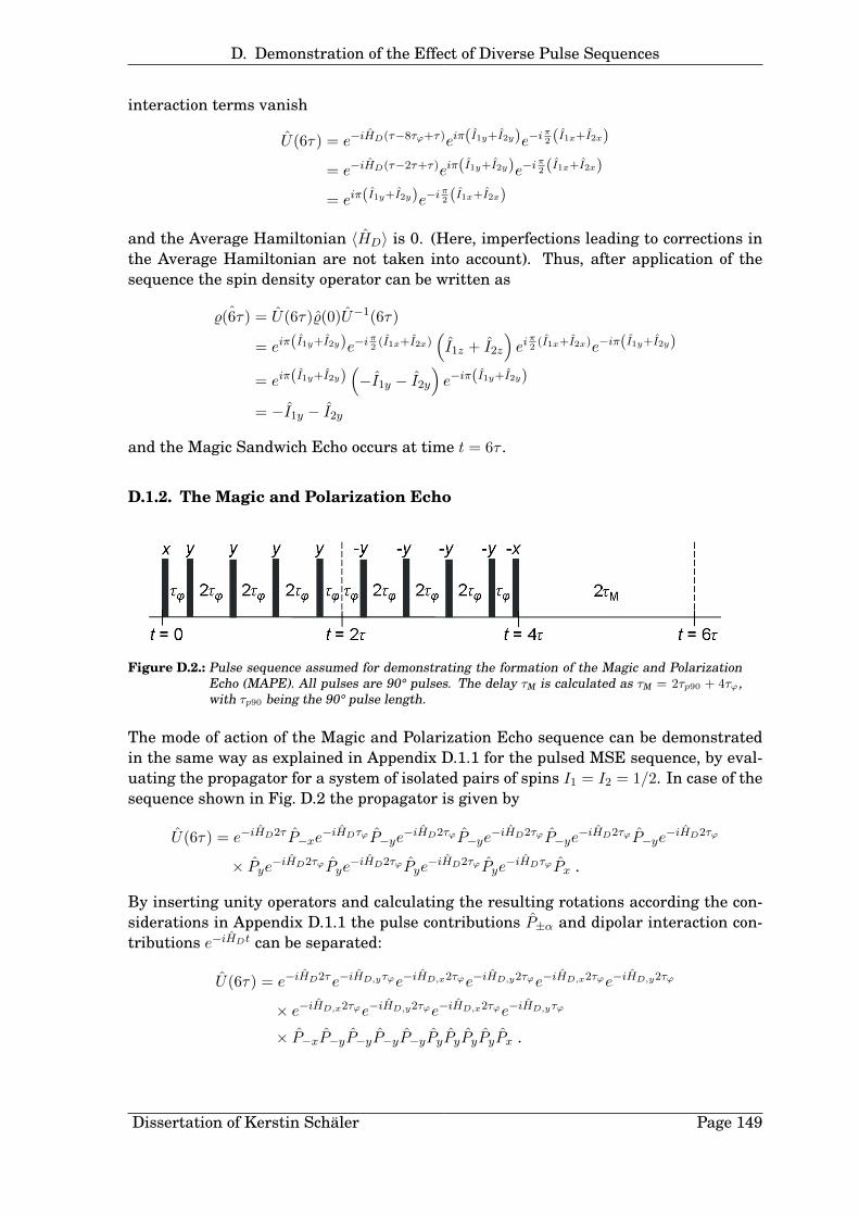
D. Demonstration of the Effect of Diverse Pulse Sequences
interaction terms vanish
U(6τ) = e−iHD(τ−8τϕ+τ)eiπ(I1y+I2y)e−iπ2 (I1x+I2x)
= e−iHD(τ−2τ+τ)eiπ(I1y+I2y)e−iπ2 (I1x+I2x)
= eiπ(I1y+I2y)e−iπ2 (I1x+I2x)
and the Average Hamiltonian 〈HD〉 is 0. (Here, imperfections leading to corrections inthe Average Hamiltonian are not taken into account). Thus, after application of thesequence the spin density operator can be written as
ˆ%(6τ) = U(6τ)%(0)U−1(6τ)
= eiπ(I1y+I2y)e−iπ2(I1x+I2x)
(I1z + I2z
)eiπ2(I1x+I2x)e−iπ(I1y+I2y)
= eiπ(I1y+I2y)(−I1y − I2y
)e−iπ(I1y+I2y)
= −I1y − I2y
and the Magic Sandwich Echo occurs at time t = 6τ .
D.1.2. The Magic and Polarization Echo
Figure D.2.: Pulse sequence assumed for demonstrating the formation of the Magic and PolarizationEcho (MAPE). All pulses are 90° pulses. The delay τM is calculated as τM = 2τp90 + 4τϕ,with τp90 being the 90° pulse length.
The mode of action of the Magic and Polarization Echo sequence can be demonstratedin the same way as explained in Appendix D.1.1 for the pulsed MSE sequence, by eval-uating the propagator for a system of isolated pairs of spins I1 = I2 = 1/2. In case of thesequence shown in Fig. D.2 the propagator is given by
U(6τ) = e−iHD2τ P−xe−iHDτϕP−ye
−iHD2τϕP−ye−iHD2τϕP−ye
−iHD2τϕP−ye−iHD2τϕ
× Pye−iHD2τϕPye−iHD2τϕPye
−iHD2τϕPye−iHDτϕPx .
By inserting unity operators and calculating the resulting rotations according the con-siderations in Appendix D.1.1 the pulse contributions P±α and dipolar interaction con-tributions e−iHDt can be separated:
U(6τ) = e−iHD2τe−iHD,yτϕe−iHD,x2τϕe−iHD,y2τϕe−iHD,x2τϕe−iHD,y2τϕ
× e−iHD,x2τϕe−iHD,y2τϕe−iHD,x2τϕe−iHD,yτϕ
× P−xP−yP−yP−yP−yPyPyPyPyPx .
Dissertation of Kerstin Schäler Page 149

D. Demonstration of the Effect of Diverse Pulse Sequences
By means of the relations D.13 and D.14 we find
U(6τ) = e−iHD2τe−i(HD,y+HD,x)8τϕ
= e−iHD2τe+iHD8τϕ
= e−iHD(2τ−8τϕ)
= e−i〈HD〉6τ
and for 2τ = 8τϕ this results in
U(6τ) = e−iHD(2τ−2τ) = E ,
with E being the unity operator, rendering 〈HD〉 = 0. (Here again, imperfections leadingto corrections in the Average Hamiltonian are not considered.)
The z-magnetization is refocused at time t = 6τ as demonstrated by writing down thedensity operator
ˆ%(6τ) = U(6τ)%(0)U−1(6τ)
= E(I1z + I2z
)E
= I1z + I2z
The filter action of the MAPE sequence, however, is based on higher order correctionsof the Average Hamiltonian, brought about by sequence imperfections as described inAppendix D.1.1. Just as in the case of the MSE sequence, these corrections prevent thecomplete refocusing of magnetization and result in an attenuation of the magnetizationecho, if the condition 6τ � 1/ωD is violated. By adapting the length of the sequence,longitudinal magnetization from regions with strong dipolar couplings can be depleted.
When calculating %(t) piecewise after every pulse one observes that the magnetizationis refocused already at t = 4τ . However, at this time the (zeroth order) Average Hamil-tonian is non-zero and the effect of dipolar couplings has not been reversed yet. Hence,for long MAPE sequences spin diffusion which is mediated by dipolar couplings (see Sec-tion 4.3) and may occur during the progression of the sequence, has not been canceledat t = 4τ . However, this is the case at t = 6τ , turning this point in time into a suitablestarting point for spin diffusion experiments.
D.2. The Double-Quantum Filter
In order to understand DQ filter action, it is beneficial to calculate the spin densityoperator piecewise after each pulse and each interval of the pulse sequence. Here, wewant to consider the evolution of a system of isolated pairs of spins I1 = I2 = 1/2, whichinteract with each other and are subjected to the DQ sequence schematically plottedin Fig. D.3. The spin system is supposed to be in thermal equilibrium in the magneticfield B0 before application of the pulse sequence. Hence, the spin density operator attime t = 0 prior to the first pulse can be written as %(0) = I1z + I2z (see Appendix C).Now, the spin density operator %(t) at time t can be estimated using the solution of the
Dissertation of Kerstin Schäler Page 150
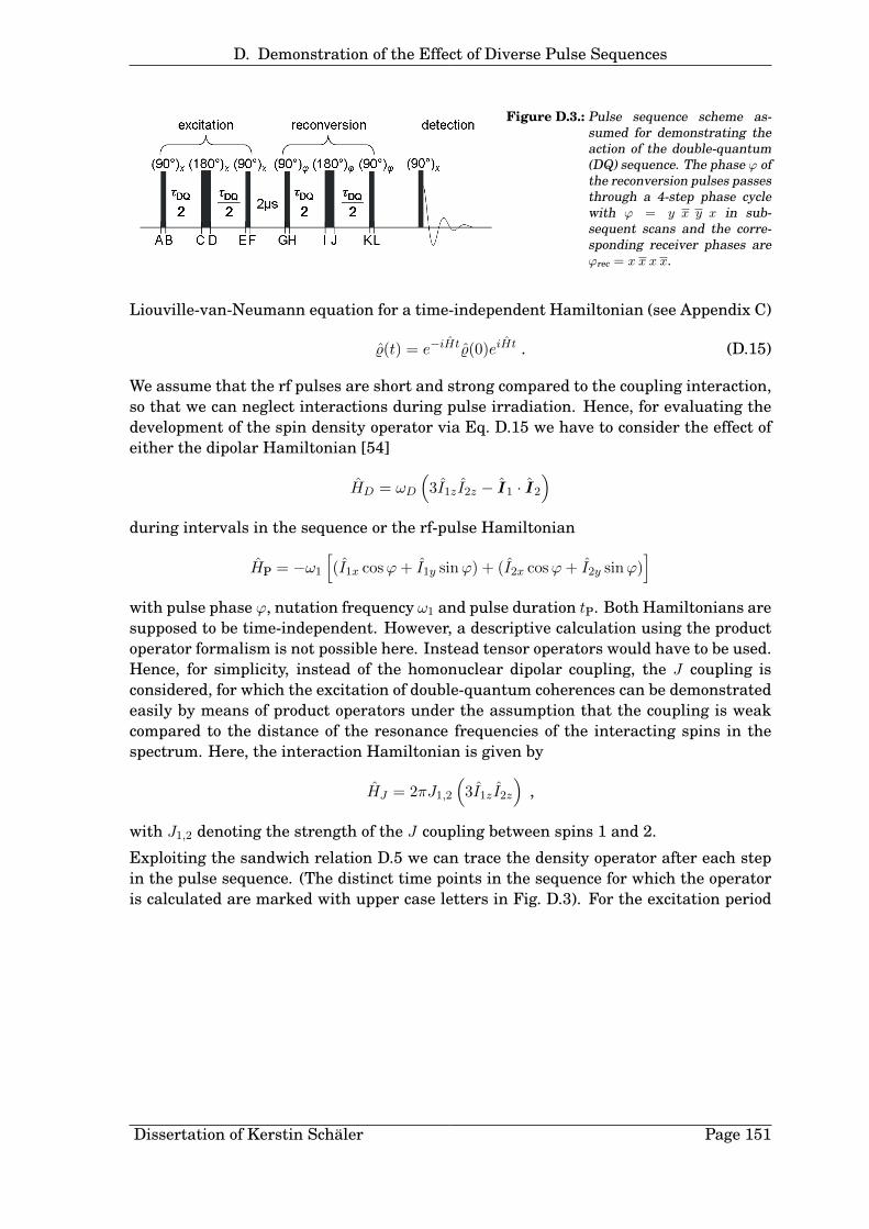
D. Demonstration of the Effect of Diverse Pulse Sequences
Figure D.3.: Pulse sequence scheme as-sumed for demonstrating theaction of the double-quantum(DQ) sequence. The phase ϕ ofthe reconversion pulses passesthrough a 4-step phase cyclewith ϕ = y x y x in sub-sequent scans and the corre-sponding receiver phases areϕrec = x x x x.
Liouville-van-Neumann equation for a time-independent Hamiltonian (see Appendix C)
%(t) = e−iHt%(0)eiHt . (D.15)
We assume that the rf pulses are short and strong compared to the coupling interaction,so that we can neglect interactions during pulse irradiation. Hence, for evaluating thedevelopment of the spin density operator via Eq. D.15 we have to consider the effect ofeither the dipolar Hamiltonian [54]
HD = ωD
(3I1z I2z − I1 · I2
)during intervals in the sequence or the rf-pulse Hamiltonian
HP = −ω1
[(I1x cosϕ+ I1y sinϕ) + (I2x cosϕ+ I2y sinϕ)
]with pulse phase ϕ, nutation frequency ω1 and pulse duration tP. Both Hamiltonians aresupposed to be time-independent. However, a descriptive calculation using the productoperator formalism is not possible here. Instead tensor operators would have to be used.Hence, for simplicity, instead of the homonuclear dipolar coupling, the J coupling isconsidered, for which the excitation of double-quantum coherences can be demonstratedeasily by means of product operators under the assumption that the coupling is weakcompared to the distance of the resonance frequencies of the interacting spins in thespectrum. Here, the interaction Hamiltonian is given by
HJ = 2πJ1,2
(3I1z I2z
),
with J1,2 denoting the strength of the J coupling between spins 1 and 2.
Exploiting the sandwich relation D.5 we can trace the density operator after each stepin the pulse sequence. (The distinct time points in the sequence for which the operatoris calculated are marked with upper case letters in Fig. D.3). For the excitation period
Dissertation of Kerstin Schäler Page 151

D. Demonstration of the Effect of Diverse Pulse Sequences
we find the following evolution of the operator:
A : I1z + I2zy (π/2)x
B : −I1y − I2yyHJ(τDQ/2)
C : −(I1y + I2y
)cos
π
2J1,2τDQ +
(2I1xI2z + 2I1z I2x
)sin
π
2J1,2τDQy (π)x
D :(I1y + I2y
)cos
π
2J1,2τDQ −
(2I1xI2z + 2I1z I2x
)sin
π
2J1,2τDQyHJ(τDQ/2)
E :(I1y + I2y
)cosπJ1,2τDQ −
(2I1xI2z + 2I1z I2x
)sinπJ1,2τDQy (π/2)x
F :(I1z + I2z
)cosπJ1,2τDQ −
(2I1xI2y + 2I1y I2x
)sinπJ1,2τDQ .
Nothing changes during the short phase-switching time of 2 µs at which the system issubject to J couplings. Thus, we end up with
G :(I1z + I2z
)cosπJ1,2τDQ︸ ︷︷ ︸
reference
−(
2I1xI2y + 2I1y I2x
)sinπJ1,2τDQ︸ ︷︷ ︸
DQ coherence
,
where the second term in the sum describes the portion of the originally longitudi-nal magnetization, which has been converted into double-quantum coherence (see Ap-pendix C), while the first term depicts the remaining z magnetization and is referred toas the reference part of the spin density operator. In order to demonstrate the evolutionin the reconversion part of the sequence both terms are considered separately. Applying
Dissertation of Kerstin Schäler Page 152

D. Demonstration of the Effect of Diverse Pulse Sequences
reconversion pulses of phase y the reference term evolves according to
G :(I1z + I2z
)cosπJ1,2τDQy (π/2)y
H :(I1x + I2x
)cosπJ1,2τDQyHJ(τDQ/2)
I :(I1x + I2x
)cos
π
2J1,2τDQ cosπJ1,2τDQ +
(2I1y I2z + 2I1z I2y
)sin
π
2J1,2τDQ cosπJ1,2τDQy (π)y
J : −(I1x + I2x
)cos
π
2J1,2τDQ cosπJ1,2τDQ −
(2I1y I2z + 2I1z I2y
)sin
π
2J1,2τDQ cosπJ1,2τDQyHJ(τDQ/2)
K : −(I1x + I2x
)cosπJ1,2τDQ cosπJ1,2τDQ −
(2I1y I2z + 2I1z I2y
)sinπJ1,2τDQ cosπJ1,2τDQy (π/2)y
L :(I1z + I2z
)cos2 πJ1,2τDQ −
(2I1xI2y + 2I1y I2x
)sinπJ1,2τDQ cosπJ1,2τDQ
and the DQ coherence converts into
G :(
2I1xI2y + 2I1y I2x
)sinπJ1,2τDQy (π/2)y
H : −(
2I1y I2z + 2I1z I2y
)sinπJ1,2τDQyHJ(τDQ/2)
I :(I1x + I2x
)sin
π
2J1,2τDQ sinπJ1,2τDQ −
(2I1y I2z + 2I1z I2y
)cos
π
2J1,2τDQ sinπJ1,2τDQy (π)y
J : −(I1x + I2x
)sin
π
2J1,2τDQ sinπJ1,2τDQ +
(2I1y I2z + 2I1z I2y
)cos
π
2J1,2τDQ sinπJ1,2τDQyHJ(τDQ/2)
K : −(I1x + I2x
)sinπJ1,2τDQ sinπJ1,2τDQ +
(2I1y I2z + 2I1z I2y
)cosπJ1,2τDQ sinπJ1,2τDQy (π/2)y
L :(I1z + I2z
)sin2 πJ1,2τDQ +
(2I1xI2y + 2I1y I2x
)sinπJ1,2τDQ cosπJ1,2τDQ
Now, the (π/2)x pulse for detection transforms(I1z + I2z
)into
(−I1y − I2y
)
Dissertation of Kerstin Schäler Page 153

D. Demonstration of the Effect of Diverse Pulse Sequences
and(
2I1xI2y + 2I1y I2x
)into
(2I1xI2z + 2I1z I2x
). As only transverse magnetization is
measurable, the terms containing products of spin operators can be discarded. For theremaining terms the receiver phase must be taken into account. With receiver phase xwe finally find the reference signal part(
I1y + I2y
)cos2(πJ1,2τDQ)
and the DQ signal part (I1y + I2y
)sin2(πJ1,2τDQ) .
Expressions for the remaining reconversion pulse phases and receiver phases are ob-tained similarly. In summary, we find the following relevant portions of the spin densityoperator:reconversion receiver reference DQpulse phase phase signal signal
y x(I1y + I2y
)cos2(πJ1,2τDQ)
(I1y + I2y
)sin2(πJ1,2τDQ)
−x −x −(I1y + I2y
)cos2(πJ1,2τDQ)
(I1y + I2y
)sin2(πJ1,2τDQ)
−y x(I1y + I2y
)cos2(πJ1,2τDQ)
(I1y + I2y
)sin2(πJ1,2τDQ)
x −x −(I1y + I2y
)cos2(πJ1,2τDQ)
(I1y + I2y
)sin2(πJ1,2τDQ)
After four subsequent scans the reference terms add up to 0 while the summation of theDQ terms yields (
I1y + I2y
)4 sin2(πJ1,2τDQ) .
Hence, after four (or a multiple of four) scans, only the fraction of originally longitudi-nal magnetization, which was converted into double-quantum coherence is transformedback into measurable transverse magnetization.
The filter effect of the DQ sequence is based on the fact, that the efficiency of conver-sion and reconversion depends on the product J1,2τDQ, e. g., in the case of isolated spinpairs, on sin2(πJ1,2τDQ) (see above). For a short excitation time τDQ appreciable signalintensity is reached only in case of a high coupling strength J1,2. Consequently, mag-netization from strongly coupled regions of the sample is selectively excited. At longerτDQ, signal from sample portions with weaker couplings can be obtained. However then,signal from strongly coupled spin pairs may have already been reduced. Yet, the situa-tion complicates for systems with more than two coupling spins with different couplingstrenghts [323].
Dissertation of Kerstin Schäler Page 154

E. PCL Densities
E. PCL Densities
PCL spin densities were obtained based on mass densities %a and %tot of amorphous andsemicrystalline PCL, respectively, measured by dilatometry over a wide temperaturerange by Crescenzi et al. [238]. In principle the mass density of the crystalline phase canbe calculated using the monomeric mass and the dimensions of the PCL unit cell. Thesedimensions, however, are temperature dependent and are known from literature only forselected temperatures [49,51,52]. Therefore, here, the mass densities for the crystallinephase, interphase (3P model) and the rigid phase, being the sum of the former two (2Pmodel), were estimated at the measurement temperatures by help of the mass fractionsfp from the FID or MSE analysis via
1
%tot=∑p
fp%p
with %tot = (1.111 ± 0.0044) g/cm3 at 27°C, (1.098 ± 0.0044) g/cm3 at 45°C and (1.097 ±0.0044) g/cm3 at 45°C [238]. In case of the 3P model the density of the interphase wasdefined to be the average of the densities of crystalline and amorphous phase. From themass densities proton spin densities were derived using Eq. 4.8. All densities used aregiven in Table E.1. The relative spin densities are related to the amorphous-phase spindensities and were used as input parameters to the fit of spin-diffusion and Saturation-Recovery data.
phase p T / °C % / g cm−3 %H / g cm−3 %H,rel
amorphous 27 1.075 ± 0.004 0.0949 ± 0.0004 1.000 ± 0.00445 1.062 ± 0.004 0.0938 ± 0.0004 1.000 ± 0.00448 1.060 ± 0.004 0.0936 ± 0.0004 1.000 ± 0.004
interphase 27 1.106 ± 0.024 0.0977 ± 0.0021 1.029 ± 0.02345 1.096 ± 0.026 0.0968 ± 0.0023 1.032 ± 0.02548 1.094 ± 0.026 0.0966 ± 0.0023 1.032 ± 0.025
crystalline 27 1.137 ± 0.044 0.1004 ± 0.0039 1.057 ± 0.04145 1.130 ± 0.048 0.0998 ± 0.0042 1.064 ± 0.04548 1.129 ± 0.049 0.0997 ± 0.0043 1.065 ± 0.046
rigid 27 1.130 ± 0.061 0.0998 ± 0.0054 1.051 ± 0.05745 1.123 ± 0.067 0.0991 ± 0.0059 1.057 ± 0.06348 1.122 ± 0.067 0.0991 ± 0.0059 1.058 ± 0.063
Table E.1.: Mass densities % and absolute and relative proton spin densities %H and %H,rel of the individualphases p in semicrystalline PCL at certain temperatures T . The uncertainties were estimatedvia error propagation from the reading uncertainty of the literature data for %a and %tot ofamorphous and semicrystalline PCL and the uncertainty of the measured sample fractions.The small uncertainties of the relative spin densities are negligible for the fits of spin-diffusionand Saturation-Recovery curves as their effect on the simulated data is only marginal.
Dissertation of Kerstin Schäler Page 155

F. Spin Diffusion
F. Spin Diffusion
F.1. Description of Magnetization Transfer Between Two Spins 1/2
Based on the following calculation it can be demonstrated easily that a magnetizationtransfer actually takes place under dipolar interaction [17]. We assume a quantum-mechanical ensemble of two spins 1 and 2 with quantum numbers I1 = I2 = 1
2 whichare located at a distance r from each other in a magnetic field being aligned along thedirection z of the coordinate system. The state of this system at time t can be describedby means of the density operator %(t). At time t = 0 only spin 1 shall exhibit magne-tization along z direction: Mz = −γ1~I1z. Thus, for t = 0 the density operator of theensemble corresponds to the z component of the spin operator of spin 1: %(0) = I1z.The dipolar Hamiltonian HD specifies the pairwise dipolar interaction between the twospins, changing the initial state and mediating spin diffusion. In the case of a weakhomonuclear coupling (compared to the Zeeman interaction) it is given by
HD = ωD(3I1z I2z − I1 · I2)
with the spin operators I1,2 and their z components I1z,2z. Via time evolution of thedensity operator by the help of the propagator U(t) = e−iHDt the state of the ensembleat time t > 0 can be calculated using a series expansion of the exponential operator [17]:
%(t) = e−iHDt%(0)e+iHDt
= %(0) + [− iHDt, %(0)] +1
2![− iHDt, [− iHDt, %(0)] ]
+1
3![− iHDt, [− iHDt, [− iHDt, %(0)] ] ] + ...
= %(0)− it
1![HD, %(0)] +
(it)2
2![HD, r1]−
(it)3
3![HD, r2] + ... ,
where the brackets denote the commutator. Inserting the Hamiltonian HD and %(0) andusing the commutators
[HD, %(0)] = iωD(I1y I2x − I1xI2y) = r1
[HD, r1] =ω2D
2(I1z − I2z) = r2
[HD, r2] = ω2Dr1 = r3
...
yields
%(t) = e−iHDtI1ze+iHDt
= I1z −it
1!(iωD(I1y I2x − I1xI2y)) +
(it)2
2!(ω2D
2(I1z − I2z))
−(it)3
3!(iω3
D(I1y I2x − I1xI2y)) +(it)4
4!(ω4D
2(I1z − I2z))− ...+ ...
Dissertation of Kerstin Schäler Page 156

F. Spin Diffusion
After rearrangement and exploitation of the sum representation of cos(ωDt) and sin(ωDt)
one obtains
%(t) =1
2I1z(1 + cos(ωDt)) +
1
2I2z(1− cosωDt) + (I1y I2x − I1xI2y) sin(ωDt) .
The first two expressions in the sum indicate that, compared to the inital state %(0) =
I1z, magnetization has been transferred from spin 1 to spin 2 to a certain extent whichdepends on the actual dipolar coupling strength ωD. Additionally, a sine-modulateddouble-quantum term has developped under dipolar interaction, which cannot be de-tected as transverse magnetization after a 90° pulse. The cosinusoidal oscillation ofdetectable magnetization in the two-spin system, expressed in the first two terms ofthe sum, will be damped in a multi-spin system due to a multitude of mutual couplingsyielding a diffusive behavior of the magnetization Mz(t) ∼
√t, if couplings of different
strenghts or between spins of differing distances exist [17].
F.2. The Simulation Program for Calculating Spin-Diffusion andSaturation-Recovery Curves
Because solving the one-dimensional spin-diffusion equation 4.11 in consideration ofT1 relaxation (see Section 4.3.2) is possible only numerically, it was transformed into afinite difference equation similar to Eq. 4.10:
M(xi, tj+1)−M(xi, tj)
∆t= Dp
M(xi−1, tj) +M(xi+1, tj)− 2M(xi, tj)
(∆x)2
+1
T1p(M0 −M(xi, tj))
M(xi, tj+1) = M(xi, tj) +Dp∆t
(∆x)2(M(xi−1, tj) +M(xi+1, tj)− 2M(xi, tj))
+∆t
T1p(M0 −M(xi, tj)) . (F.1)
Here, M denotes the space and time-dependent magnetization. The variables of spacexi and time tj adopt discrete values with equidistant increments ∆x = xi+1 − xi and∆t = tj+1−tj , respectively. M0 designates the equilibrium magnetization of the T1 relax-ation process. According to Eq. F.1 the simulation program written by Prof. H. Schneidercalculates M(xi, tj+1) stepwise for every domain p. By reason of symmetry, it is suffi-cient to conduct the computation for half of the repeat unit (see Fig. 7.6 (b)) and tointroduce the following periodic symmetry and boundary conditions to take into accountthe lamellar structure of the system [139,141]:
• at the symmetry planes s (see Fig. 7.6 (a)), with space coordinate xs, magnetizationis not allowed to change locally: M(xs, t) = M(xs+1, t) = M(xs−1, t)
• at the boundary planes b located at xb (see Fig. 7.6 (b)) between two phases p1 andp2 magnetization must develop continuously: Mp1(xb, t) = Mp2(xb, t),
• boundary planes b must not act as magnetization sources or sinks, i. e. the flux of
Dissertation of Kerstin Schäler Page 157

F. Spin Diffusion
magnetization has to be continuous there:
%H,p1Dp1Mp1(xb, t)−Mp1(xb−1, t)
xb − xb−1= %H,p2Dp2
Mp2(xb+1, t)−Mp2(xb, t)
xb+1 − xb
The last expression contains the phase-specific proton spin density %H,p (see Section 4.1).The observable in the experiments is the total magnetization Mp(τdiff) in each phase p.An equivalent parameter Mp(tj) can be derived from the simulation by summing upthe magnetization M(xi, tj) of every discrete position xj in a phase p, multiplied by thecorresponding proton spin density %H,p. Here, the time coordinate tj corresponds to themixing time τdiff in the experimental setup. Depending on the initial values of the mag-netization in the individual phases Mp(0) and the equilibrium magnetization M0,1 themagnetization development in spin-diffusion and Saturation-Recovery experiments canbe computed. In order to compare simulated and measured data the magnetization de-velopment has to be calculated starting from a given initial distribution and proceedinguntil the equilibrium distribution is reached. The accuracy of the calculation dependson the choice of the space and time increments ∆x and ∆t. Following from Eq. F.1 thevalue of the expression (Dp∆t)/(∆x)2 must be limited. For convergence a value smallerthan 0.5 is necessary. All fits and simulations represented herein were conducted withequal increments ∆x = 0.5 Å and ∆t = 2 µs to achieve comparable results.
F.3. Derivation of the Source Domain Size by means of the Initial RateApproximation
The analytical solution of the spin-diffusion equation for a scenario of a finite sourceregion from which magnetization is transferred into an infinite sink region can be usedto deduce an expression for the source domain size in a two-phase polymer system. Inorder to explain this idea, the derivation of the IRA equation shall be described herein detail according to the considerations of Clauss et al. [139]. The space coordinate inthe one-dimensional scenario is denoted by x and the time by t. In the experimentalsetup the time coordinate t corresponds to the mixing time τdiff. When magnetizationemanates from a point-shaped source at the position x = r, the Gaussian function
M(x, t) =M0√4πDt
e−(x−r)24Dt (F.2)
for the magnetization M(x, t) is a solution of the spin-diffusion equation 4.11 for a con-stant spin-diffusion coefficientD and a constant proton spin density %H over all positionsx. Here, M0 is the initial magnetization at x = r.
A finite magnetization source at −r0 < x < r0 between infinite sinks at |x| > r0 at t = 0
can be represented by an infinite number of point-shaped sources uniformly distributedover all positions −r0 < x < r0. Thus, in this case a superposition of Gaussian functions
1The value of M0 is 0 for the calculation of spin-diffusion curves due to the z filter used in the experiments(see Section 4.3.2) and 1 for the calculation of Saturation-Recovery curves.
Dissertation of Kerstin Schäler Page 158

F. Spin Diffusion
F.2 at r = −r0 . . . r0 solves Eq. 4.11:
M(x, t) =
∫ r0
−r0
M0√4πDt
e−(x−r)24Dt dr = −M0√
π
∫ x−r0√4Dt
x+r0√4Dt
e−z2dz
= −M0√π
(∫ 0
x+r0√4Dt
e−z2dz +
∫ x−r0√4Dt
0e−z
2dz
)
=M0√π
(∫ x+r0√4Dt
0e−z
2dz +
∫ − x−r0√4Dt
0e−z
2dz
)
=M0
2erf
(r0 + x√
4Dt
)+M0
2erf
(r0 − x√
4Dt
), (F.3)
where erf(x) is the error function defined as
erf(x) =
∫ x
0
2
πe−z
2dz .
Equation F.3 is symmetric with respect to x = 0 and contains one term each for themagnetization transfer via the source-sink interfaces at x = −r0 and at x = r0. At t = 0
it results in a box function with M(x, t = 0) = M0 for |x| < r0 and M(x, t = 0) = 0 other-wise. With increasing time the magnetization at x = 0 and the magnetization gradientnear the interfaces decreases until at t → ∞ a uniform distribution of magnetization isreached for all x with M(x)→ 0. However, as a result of the error function properties atshort times t � (r20/4D) the first term in Eq. F.3 is approximately constant in time andspace for x > 0 while the second one yields a constant at positions x < 0:
M(x > 0, t� (r20/4D)) =M0
2+M0
2erf(
r0 − x√4Dt
) (F.4)
M(x < 0, t� (r20/4D)) =M0
2erf(
r0 + x√4Dt
) +M0
2(F.5)
These expressions equal the solution of Eq. 4.11 for an infinite source either at x < r0(Eq. F.4) or at x > −r0 (Eq. F.5). (Alternatively, these solutions can also be derived bysuperposing the solutions for an infinite number of point-shaped sources in the corre-sponding source regions.) Hence, at short times the magnetization close to an interfacedevelops as if no other interface would exist (cf. Fig. 7.18 (a)). It therefore suffices toconsider only the magnetization development near one interface even if many more ofthe same kind are present. Expressions of the type of Eqs. F.4 or F.5 can thereforealso be used to describe the short-time behavior of magnetization in periodic systems ofalternating source and sink regions as present in the 2P model.
Now the solution shall be specified for a periodic two-phase polymer system containingsource domains A and sink domains B with individual spin-diffusion coefficients DAand DB and proton spin densities %H,A and %H,B which are each constant within therespective phase. For this purpose the solutions for each phase have to be adapted tofulfill certain initial and boundary conditions equal to those given in Section F.2. Here,they are presented in a continuous form:
• At t = 0 the source domain A contains the full magnetization, i. e.
Dissertation of Kerstin Schäler Page 159

F. Spin Diffusion
MA(x, t = 0) = M0 and MB(x, t = 0) = 0,
• at the boundary surface r0 between source and sink domain the magnetizationdevelops continuously, i. e. MA(r0, t) = MB(r0, t),
• at the boundary surface r0 the magnetization flux is continuous, i. e.
−DA%H,A∂MA(r0, t)
∂x= −DB%H,B
∂MB(r0, t)
∂x
The differences in spin-diffusion coefficients and spin densities of the phases A and Bresult in changes of the absolute values of the magnetization compared to the expres-sions F.4 and F.5, while the principal structure of the solution is preserved. Thereforefor both phases a generalized ansatz is made:
MA(x, t) = EA + FA erf
(x− r0√
4Dt
)for domain A at x < r0 and (F.6)
MB(x, t) = EB + FB erf
(x− r0√
4Dt
)for domain B at x > r0. (F.7)
Applying the conditions above to these equations and taking into account the propertiesof the error function
erf(x→ ±∞) = ±1
erf(0) = 0
d
dxerf(y(x)) =
d
dx
∫ y(x)
0
2
πe−z
2dz =
d
dx(F (y(x))− F (0))
=dF (y)
dy
dy(x)
dx=
2
πe−y(x)
2 dy(x)
dx,
with F (y) being the antiderivative of(
2πe−y2)
, one obtains
EA − FA = M0 ,EB + FB = 0 ,
EA = EB and√DA%H,AFA =
√DB%H,BFB .
Rearranging these expressions and inserting them into Eq. F.6 and Eq. F.7 yields [139]
MA(x, t) =M0%H,A
√DA
%H,A√DA + %H,B
√DB−
M0%H,B√DB
%H,A√DA + %H,B
√DB
erf
(x− r0√
4DAt
)and
MB(x, t) =M0%H,A
√DA
%H,A√DA + %H,B
√DB−
M0%H,A√DA
%H,A√DA + %H,B
√DB
erf
(x− r0√
4DBt
)=
M0%H,A√DA
%H,A√DA + %H,B
√DB
erfc
(x− r0√
4DBt
)with erfc(x) = 1 − erf(x). For DA = DB and %H,A = %H,B Eq. F.4 results again from bothsolutions.
The total magnetization MB(t) of the sink at short times t can be estimated by summing
Dissertation of Kerstin Schäler Page 160

F. Spin Diffusion
up the magnetization MB(x, t) of all spins on cross-sectional areas AS parallel to theinterface between A and B for positions x > r0 in consideration of the spin density:
MB
(t� r20
4DB
)≈ %H,B
∫ ∞r0
MB(x, t)ASdx
= %H,BAS
∫ ∞r0
M0%H,A√DA
%H,A√DA + %H,B
√DB
erfc
(x− r0√
4DBt
)dx
=2√π
ASM0%H,A%H,B√DA√DB(
%H,A√DA + %H,B
√DB) √t (F.8)
Here, the relation∫∞x erfc(z)dz = 1√
πe−x
2 − x erfc(x) was used. Correspondingly, for thetotal magnetization MA(t) of the source one finds
MA
(t� r20
4DA
)≈ %H,A
∫ r0
0MA(x, t)ASdr
MA(t = 0) ≈ %H,A
∫ r0
0MA(x, t = 0)ASdr = %H,AM0ASr0 (F.9)
As visible in Eq. F.8 for short times the sink magnetization follows a√t dependence.
The approximated total intensity MB(t � r204DB
) reaches the value of the total initialmagnetization MA(t = 0) of the system at a characteristic time t0:
MB
(t� r20
4DB,√t0
)= MA(t = 0)
2√π
ASM0%H,A%H,B√DA√DB
%H,A√DA + %H,B
√DB
√t0 = r0%H,AASM0 (F.10)
The same relation F.10 can also be derived from the expression for the source magneti-zation via MA
(t� r20
4DA,√t0
)= 0 .
For a given value of√t0, Eq. F.10 can finally be used to determine r0 which in our
scenario corresponds to half of the source domain thickness dA:
dA = 2r0 =4√π
√DA√DB(
%H,A%H,B
√DH,A +
√DB
)√t0 . (F.11)
F.4. Effects of PCL Domain-Thickness Distributions on Spin Diffusion
It is known from literature, that domain thicknesses in semicrystalline polymers dependon molecular weight, crystallization temperature Tc (0.5 K) and the thermal history ofthe sample [10]. The PCL sample investigated by spin-diffusion experiments (see Sec-tion 7.2) is polydisperse and slight deviations of Tc could not be avoided. Hence, it seemsself-evident that distributions of domain sizes exist here. Actually, this is confirmed bythe SAXS results, where broad peaks were detected in the interface-distance distribu-tion function. Interestingly, in PCL the distribution width of the amorphous-phase do-main thicknesses is significantly larger than the one obtained for the crystalline lamel-lae (see Table 7.1). This is presumed to be a feature of crystal-fixed polymers [218].
Dissertation of Kerstin Schäler Page 161

F. Spin Diffusion
The fact that domain sizes differ within the phases of a polymer sample seems to beaccepted in literature concerning SAXS experiments (see, e. g., Ref. [324]) and has alsobeen addressed in NMR literature [89, 116, 250]. However, only a few works deal withthe impact of domain-size distributions on spin-diffusion data in more detail. As thedomain thicknesses influence the shape of the spin-diffusion curves, the existence of dif-ferent thicknesses within the phases may alter the data in a complex way [325]. There-fore it shall be discussed here, whether thickness distributions could have induced thediscrepancies between measured data and fit data described in Section 7.3.
Domain-size distributions arise when each polymer domain exhibits a constant thick-ness over its complete lateral extension while different regions of an individual phaseexhibit non-uniform domain sizes (see Fig. F.1 (a)), but also when there are thicknessfluctuations within distinct domains resulting in non-planar interfaces between them(see Fig. F.1 (b)). Both scenarios may occur in PCL. The analysis of the SAXS data relieson the former concept, the effects of which shall be investigated in this section, whileconsequences of the latter are discussed in Section 7.5.
(a) (b)
Figure F.1.: Two-phase scenarios showing non-uniform domain thicknesses (see text). The labels c and adesignate the crystalline and amorphous phase, respectively.
The simulation program (see Section 7.3 and Appendix F.2) allows to simulate spin-diffusion curves for non-uniform domain sizes as depicted in Fig. F.1 (a). Here, for eachphase p random domain thicknesses are generated which fluctuate around a given meanvalue dp,ave following a Gaussian distribution with an adjustable relative distributionwidth σrel,p = σp/dp.
Performing simulations for the 2P model with exactly the same program as describedhere, Mauri et al. have shown that distributions of domain sizes of the rigid and mobile-amorphous phase with relative widths σrel,p up to 0.75 cause only slight changes in theshape of the spin-diffusion curves with root-mean-square deviations rms smaller than3% [8]. From their work they concluded that the domain thicknesses and spin-diffusioncoefficients obtained from the fits do not deviate too much from the true values, whenrelative thickness fluctuations are smaller than σrel,p ≈ 0.2.
However, according to the SAXS results, in PCL these fluctuations can be larger than0.2 (see Table 7.1). In order to estimate the effect of thickness distributions for thespecific case of PCL, simulations have been performed here for the 2P and the 3P modelwith realistic parameter values for PCL at 45°C and different domain-size distributionwidths (σrel,p = 0.1, 0.3, 0.5 and 0.6 for the 2P model and σrel,p = 0.1 and 0.5 for the 3Pmodel), on the one hand by assuming domain-size fluctuations in a single phase onlyand on the other hand by varying the sizes in several or all phases, simultaneously. Forevery distribution width three different sets of domain thicknesses were tried for the2P system and only one for the 3P system. When generating the random thicknessesfor the individual polymer phases, it was checked that the standard deviation from the
Dissertation of Kerstin Schäler Page 162

F. Spin Diffusion
corresponding mean thickness was in accordance with the settled distribution width.
The thickness distributions expectedly induced changes in the shape of the spin-diffusionand Saturation-Recovery curves, which increased with rising distribution width. Fordomain-size distributions in several polymer phases at the same time the effects of thethickness fluctuations of the single phases added up. The following effects could bedetected (see Fig. F.2):
• Changes due to a distribution of mobile-amorphous-phase, crystalline-phase andrigid-phase domain thicknesses followed the same trend and for the same distri-bution width they also exhibited the same extent.
• The effects of a distribution of interphase domain thicknesses were negligible asthe interphase fraction in the simulation model was small.
• The Saturation-Recovery curves exhibited only small changes due to thicknessfluctuations in the region of decreasing slope.
• The most striking effect on the shape of the spin-diffusion curves was a decreaseof the maximum intensity of the sink-domain signal with increasing distributionwidth of the domain size of the mobile-amorphous, crystalline or rigid phase, com-bined with a slight shift of the maximum to shorter mixing times τdiff. At the sametime the source domain signal exhibited a slightly retarded decay and/or an in-creased magnetization level at large mixing times. The latter was predicted byCheung, who investigated the implications of disorder in polymer morphology onthe analytical solution of the spin-diffusion equation [325].
These shape variations were rather small but systematic (see Fig. F.3). The rms devia-tion between simulated spin-diffusion curves calculated for constant domain thicknessesand for a realistic distribution of domain sizes in PCL, derived via
rms =1
n
√√√√ n∑i=1
(I2i − I1i)2(I1i)2
,
amounts to 0.4% to 2.4% only and is in the range of the values given by Mauri et al. Inthe equation n denotes the number of data points in the spin-diffusion curves and I1iand I2i represent the intensities of the two curves which are compared (see Fig. F.3).
To check the consequences of thickness distributions on the parameter values from a fitusing a model with constant domain sizes, spin-diffusion and Saturation-Recovery datawere simulated assuming realistic distribution widths for the thicknesses of the crys-talline and mobile-amorphous domains in PCL at 45°C (cf. Table 7.1): σrel,c = 0.11 andσrel,a = 0.52. The value for the interphase was chosen to be σrel,i = 0.11 as well. Now asimultaneous fit to these data was performed using the 2P or 3P model with the param-eter values underlying the simulation used as initial values for the fit. Here, the meanthicknesses from the simulation served as domain size parameter values. The fitting ofsimulated data which were generated for constant domain sizes worked perfectly welland reproduced the simulation parameters, also when the initial values were changed.Keeping the spin-diffusion coefficients and T1 values fixed in the fit to data simulatedfor a distribution of domain sizes, fit curves were obtained which matched the simulatedones acceptably well but brought about too large thickness values for all three polymerphases. The thicknesses da and dc were ∼14% higher than defined in the simulation, di
Dissertation of Kerstin Schäler Page 163

F. Spin Diffusion
Figure F.2.: Demonstration of the effects of domain-size distributions on simulated data from crystalline-phase-selected (upper left) and mobile-amorphous-phase-selected (upper right) spin-diffusionand Saturation-Recovery (lower left) experiments. The simulations were performed for a 3Pmodel and different combinations of relative thickness distribution widths σrel,a,i,c using theparameters shown in the lower right of the figure and the relative spin densities %H,a = 1, %H,i =1.034 and %H,c = 1.067. The subscripts a, i and c designate the mobile-amorphous phase, inter-phase and crystalline phase, respectively. The arrows depict curve variations for increasingdistribution widths.
deviated by ∼ 8%. These findings agree with the deviation of ∼10% stated by Mauri etal. [8]. As for PCL the aim was to derive spin-diffusion coefficients, in a next step thedomain sizes were fixed in the fit, while the diffusion coefficients were free parameters.The curves from fit and simulation matched well for the source domain, but the fit couldnot reproduce the rise of the sink curve completely (see Fig. F.4). However, when fittingnoisy experimental data such small differences would not be evident.
Nevertheless, the systematic changes in the curve shape mentioned above induce mod-ifications of the fit parameters compared to the values used for the simulation. Thereduced sink-phase intensity is compensated in the fit by a systematic and partly sig-nificant variation of the spin-diffusion coefficients. The fit pretended values of Da whichwere too low by a factor of 0.67 to 0.77 compared to the true values used in the sim-ulation. Stable fits also yielded too small values of Drig differing from the value of thesimulation by the same factor as obtained for Da. On the other hand, when the initial fitparameters were chosen in an unfavorable way the value of Drig increased dramaticallyup to implausibly high values larger than 2 nm2/ms but no stable fit was obtained. Suchhigh values of Drig should be discarded when fitting experimental data as they wereprovoked artificially by the domain-size distributions.
Stable fits using the 3P model were obtained for reduced values of Da and Dc and in-
Dissertation of Kerstin Schäler Page 164

F. Spin Diffusion
Figure F.3.: Relative difference betweenthe intensities of spin-diffusioncurves simulated for constantdomain thicknesses (simula-tion 1 with intensity I1) and fora realistic distribution of do-main sizes (simulation 2 withintensity I2) for PCL at 45°C.The intensities were calcu-lated using the spin-diffusioncoefficients given in the plot.The remaining simulation pa-rameters are the same as inFig. F.2.
Figure F.4.: Comparison of spin-diffusiondata simulated for a realis-tic distribution of domain sizes(see legend) with two fits tothese data, using a fit modelwhich ignores the size distri-bution. In the fits the do-main thicknesses were fixedto the average values appliedin the simulation and givenin Fig. F.2. The spin densi-ties used are indicated there aswell.
creased values of Di. However, it is not possible to estimate to which extent the valuesof Dc and Di deviated from the ones of the simulation, as these parameters stronglydepended on each other and both had similar effects on the spin-diffusion curves. A lowvalue of Dc induced a high value of Di and vice versa. This way, stable fits were possiblefor large values of Dc > 0.6 nm2/ms on the one hand and for Dc < Di on the other hand(see Fig. F.4). The latter seems physically unlikely because, due to less anisotropic chainmobility in the interphase, the dipolar coupling strength and therefore also the spin-diffusion coefficient should be smaller than in the crystallites. The interdependence ofall three parameters Dc, Di and Da is depicted in Fig. F.5 (b).
Compared to the values of the simulation, the T1 values did not change appreciably inthe fit for the 2P model. Yet, from fits using the 3P model only T1a could be determinedprecisely. Similar to the interdependence of the diffusion coefficients, also T1i and T1cwere coupled, enabling large ranges of possible fit values including T1i > T1c. This re-lation seems doubtful because for the apparent T1 values derived from the initial risesof the Saturation-Recovery curves the inverted trend was observed (see Fig. 5.3 in Sec-tion 5.1).
In fact, interdependencies between the fit results for Di and Dc as well as T1i and T1chave been found in the fits of measured data for PCL (see Fig. F.5 (a)). As shown here,dubious combinations of fit parameters such as Dc < Di or T1c < T1i can be discarded asfitting artifacts resulting from neglected domain-size distributions.
In summary, due to the domain-size fluctuations within the polymer phases, stable
Dissertation of Kerstin Schäler Page 165

F. Spin Diffusion
(a) (b)
Figure F.5.: Interdependence between the parameter values of the spin-diffusion coefficientsDc,Da andDi
of crystalline phase, mobile-amorphous phase and interphase. The values were obtained fromfits to experimental (a) and simulated (b) data using the program described in Section 7.3 forthe 3P model, keeping the domain-size parameters fixed. The simulated data were calculatedby means of the same program with parameter values given in Fig. F.2 but taking into accounta realistic distribution of domain thicknesses (see text). The solid grey lines are guides to theeye. The red squares mark the set of spin-diffusion coefficients used for the simulation in (b).Crossed symbols in (a) depict values from fits with minor but still acceptable fit quality.
fits to the experimental data will yield average values of mobile-amorphous-phase andcrystalline-phase spin-diffusion coefficients, which are lower than actually present inthe sample, whereas the coefficient of the interphase will rather be determined too large.The true values cannot be obtained by means of the fit used here. However, a set of suchassociated apparent values nevertheless permits the determination of correct averagedomain sizes, which is usually the aim of spin-diffusion experiments. In this sense,neglecting domain-size distributions when fitting PCL spin-diffusion data is justifieddespite of a large distribution width of the mobile-amorphous-phase domain sizes.
For the experimental spin-diffusion curves in the 2P model a shift of the initial rise anddecay was found for the sink and source signal intensity as compared to the simula-tion (see Sections 7.3 and 7.4). Yet, as shown here, domain-size distributions do notchange the initial rise or decay time appreciably and thus cannot be a reason for such adelayed magnetization development. Also the unexpected shape of the measured inter-phase signal in the MAPE experiments is not caused by thickness fluctuations, as theseinfluence the interphase signal only marginally. Furthermore, the maximum sink-curvesignal intensities from MAPE-filtered and DQ-filtered experiments both decrease to thesame extent due to realistic domain-size distributions in PCL (cf. Fig. F.2). The attemptto fit both sets of data with one set of spin-diffusion coefficients thus fails also whendomain-size distributions are taken into account.
Dissertation of Kerstin Schäler Page 166

Bibliography
Bibliography
[1] Pfeifer, H. (1999) A short history of nuclear magnetic resonance spectroscopy andof its early years in Germany. Magn. Reson. Chem., 37, S154–S159.
[2] Ernst, R. R. (2010) Zurich’s Contributions to 50 Years Development of Bruker.Angew. Chem., Int. Ed., 49, 8310–8315.
[3] Nelson, F. A. and Weaver, H. E. (1964) Nuclear Magnetic Resonance Spectroscopyin Superconducting Magnetic Fields. Science, 146, 223–232.
[4] Lewandowski, J. R., Dumez, J.-N., Akbey, U., Lange, S., Emsley, L., and Oschkinat,H. (2011) Enhanced Resolution and Coherence Lifetimes in the Solid-State NMRSpectroscopy of Perdeuterated Proteins under Ultrafast Magic-Angle Spinning. J.Phys. Chem. Lett., 2, 2205–2211.
[5] Samoson, A., Tuherm, T., Past, J., Reinhold, A., Anupõld, T., and Heinmaa, I.(2004) New Horizons for Magic-Angle Spinning NMR. Topics in Current Chem-istry, Springer-Verlag Berlin Heidelberg.
[6] Nishiyama, Y., Endo, Y., Nemoto, T., Utsumi, H., Yamauchi, K., Hioka, K., andAsakura, T. (2011) Very fast magic angle spinning 1H-14N 2D solid-state NMR:Sub-micro-liter sample data collection in a few minutes. J. Magn. Reson., 208,44–48.
[7] Brown, S. P. (2012) Applications of high-resolution 1H solid-state NMR. SolidState Nucl. Magn. Reson., 41, 1–27.
[8] Mauri, M., Thomann, Y., Schneider, H., and Saalwächter, K. (2008) Spin-diffusionNMR at low field for the study of multiphase solids. Solid State Nucl. Magn. Re-son., 34, 125–141.
[9] Mandelkern, L. (1990) The Structure of Crystalline Polymers. Acc. Chem. Res.,23, 380–386.
[10] Strobl, G. (2007) The physics of polymers: concepts for understanding their struc-tures and behavior. Springer, 3., rev. and expanded edn.
[11] Iwata, K. (2002) Role of entanglement in crystalline polymers 1. Basic theory.Polymer, 43, 6609–6626.
[12] Kitamaru, R., Horii, F., and Murayama, K. (1986) Phase Structure of LamellarCrystalline Polyethylene by Solid-state High-Resolution 13C NMR: Detection ofthe Crystalline-Amorphous Interphase. Macromolecules, 19, 636–643.
[13] Mandelkern, L., Alamo, R. G., and Kennedy, M. A. (1990) Interphase Thickness ofLinear Polyethylene. Macromolecules, 23, 4721–4723.
[14] Cheng, J. L., Fone, M., Reddy, V. N., Schwartz, K. B., Fisher, H. P., and Wunderlich,B. (1994) Identification and quantitative analysis of the intermediate phase in alinear high-density polyethylene. J. Polym. Sci., Part B: Polym. Phys., 32, 2683–2693.
[15] Schick, C., Wurm, A., Merzlyakov, M., Minakov, A., and Marand, H. (2001) Crys-tallization and melting of polycarbonate studied by temperature-modulated DSC(TMDSC). J. Therm. Anal. Calorim., 64, 549–555.
[16] Flory, P. J. (1962) On the morphology of the crystalline state in polymers. J. Am.
Dissertation of Kerstin Schäler Page 167

Bibliography
Chem. Soc., 84, 2857–2867.
[17] Schmidt-Rohr, K. and Spiess, H. W. (1994) Multidimensional Solid-State NMRand Polymers. Academic Press.
[18] Schick, C., Dobbertin, J., Potter, M., Dehne, H., Hensel, A., Wurm, A., Ghoneim,A. M., and Weyer, S. (1997) Separation of components of different molecular mo-bility by calorimetry, dynamic mechanical and dielectric spectroscopy. J. ThermalAnal., 49, 499–511, Proceedings of the 11th International Congress on ThermalAnalysis and Calorimetry.
[19] Schick, C., Wurm, A., and Mohamed, A. (2001) Vitrification and devitrification ofthe rigid amorphous fraction of semicrystalline polymers revealed from frequency-dependent heat capacity. Colloid Polym. Sci., 279, 800–806.
[20] Armitstead, K., Goldbeck-Wood, G., and Keller, A. (1992) Polymer crystallizationtheories. Adv. Polym. Sci., 100, 221–312.
[21] Lauritzen, J. I. and Hoffman, J. D. (1960) Theory of formation of polymer crys-tals with folded chains in dilute solution. J. Res. Natl. Bur. Stand., Sect. A: Phys.Chem., 64, 73–102.
[22] Hoffman, J. and Miller, R. (1997) Kinetics of crystallization from the melt andchain folding in polyethylene fractions revisited: Theory and experiment. Polymer,38, 3151–3212.
[23] Strobl, G. (2000) From the melt via mesomorphic and granular crystalline layersto lamellar crystallites: A major route followed in polymer crystallization? Eur.Phys. J. E, 3, 165–183.
[24] Sadler, D. M. (1987) New explanation for chain folding in polymers. Nature, 326,174–177.
[25] Konishi, T., Sakatsuji, W., Fukao, K., and Miyamoto, Y. (2011) Polymer crystal-lization mechanism through a mesomorphic state. Phys. Rev. B, 84, 132102.
[26] Muthukumar, M. (2007) Shifting paradigms in polymer crystallization. Lect.Notes Phys., 714, 1–18.
[27] Olmsted, P. D., Poon, W. C. K., McLeish, T. C. B., Terrill, N. J., and Ryan, A. J.(1998) Spinodal-assisted crystallization in polymer melts. Phys. Rev. Lett., 81,373–376.
[28] Robelin-Souffaché, E. and Rault, J. (1989) Origin of the long period and crys-tallinity in quenched semicrystalline polymers. 1. Macromolecules, 22, 3581–3594.
[29] Ou-Yang, W.-C., Li, L.-J., Chen, H.-L., and Hwang, J. C. (1997) Bulk crystallizationBehavior of Poly(ε-caprolactone) with a Wide Range of Molecular Weight. Polym.J., 29, 889–893.
[30] Jenkins, M. J. and Harrison, K. L. (2006) The effect of molecular weight on thecrystallization kinetics of polycaprolactone. Polym. Adv. Technol., 17, 474–478.
[31] Bu, H. S., Gu, F. M., Bao, L. R., and Chen, M. (1998) Influence of entanglementson crystallization of macromolecules. Macromolecules, 31, 7108–7110.
[32] Psarski, M., Piorkowska, E., and Galeski, A. (2000) Crystallization of polyethy-lene from melt with lowered chain entanglements. Macromolecules, 33, 916–932.
Dissertation of Kerstin Schäler Page 168

Bibliography
[33] Umemoto, S. and Okui, N. (2002) Master curve of crystal growth rate and itscorresponding state in polymeric materials. Polymer, 43, 1423–1427.
[34] Hu, W., Frenkel, D., and Mathot, V. B. F. (2003) Intramolecular nucleation modelfor polymer crystallization. Macromolecules, 36, 8178–8183.
[35] Xiao, Z. G., Sun, Q., Xue, G., Yuan, Z. R., Dai, Q. P., and Hu, Y. L. (2003) Thermalbehavior of isotactic polypropylene freeze-extracted from solutions with varyingconcentrations. Eur. Polym. J., 39, 927–931.
[36] Mandelkern, L. (2004) Crystallization kinetics of homopolymers: overall crystal-lization: a review. Biophys. Chem., 112, 109–116.
[37] Hikosaka, M., Watanabe, K., Okada, K., and Yamazaki, S. (2005) Topologicalmechanism of polymer nucleation and growth - The role of chain sliding diffusionand entanglement. Interphases and mesophases in polymer crystallization III, vol.191 of Advances in Polymer Science, pp. 137–186.
[38] Lippits, D. R., Rastogi, S., Hohne, G. W. H., Mezari, B., and Magusin, P. C. M. M.(2007) Heterogeneous distribution of entanglements in the polymer melt and itsinfluence on crystallization. Macromolecules, 40, 1004–1010.
[39] Traficante, D. (1996) Relaxation: An introduction. Grant, D. M. and Harris, R. K.(eds.), Encyclopedia of Nuclear Magnetic Resonance, John Wiley & Sons Ltd.
[40] Saalwächter, K. (2007) Proton multiple-quantum NMR for the study of chain dy-namics and structural constraints in polymeric soft materials. Prog. Nucl. Magn.Reson. Spectrosc., 51, 1–35.
[41] Vaca Chávez, F. and Saalwächter, K. (2011) Time-Domain NMR Observation ofEntangled Polymer Dynamics: Universal Behavior of Flexible Homopolymers andApplicability of the Tube Model. Macromolecules, 44, 1549–1559.
[42] Boyd, R. H. (1985) Relaxation processes in crystalline polymers: experimentalbehavior - a review. Polymer, 26, 323–347.
[43] Rault, J. (1997) The αc Transition in Semicrystalline Polymers: A New Look atCrystallization Deformation and Aging Process. J. M. S. - Rev. Macromol. Chem.Phys., C37, 335–387.
[44] Hu, W.-G. and Schmidt-Rohr, K. (1999) Polymer ultradrawability: the crucial roleof α-relaxation chain mobility in the crystallites. Acta Polym., 50, 271–285.
[45] Syi, J.-L. and Mansfield, M. L. (1988) Soliton model of the crystalline α relaxation.Polymer, 29, 987–997.
[46] Mark, J. E. (ed.) (2007) Physical Properties of Polymers Handbook. Springer, 2ndedn.
[47] Woodruff, M. A. and Hutmacher, D. W. (2010) The return of a forgotten polymer -polycaprolactone in the 21st century. Prog. Polym. Sci., 35, 1217–1256.
[48] Röthemeyer, F. and Sommer, F. (2006) Kautschuktechnologie. Carl Hanser Verlag,2nd ed. edn.
[49] Bittiger, H., Marchessault, R. H., and Niegisch, W. D. (1970) Crystal Structure ofPoly-ε-caprolactone. Acta Crystallogr., Sect. B: Struct. Crystallogr. Cryst. Chem.,B 26, 1923–1927.
Dissertation of Kerstin Schäler Page 169

Bibliography
[50] Bunn, C. W. and Alcock, T. C. (1945) The texture of polyethylene. Trans. FaradaySoc., 41, 317–325.
[51] Chatani, Y., Okita, Y., Tadokoro, H., and Yamashita, Y. (1970) Structural Studiesof Polyesters. III. Crystal Structure of Poly-ε-caprolactone. Polym. J., 1, 555–562.
[52] Hu, H. L. and Dorset, D. L. (1990) Crystal structure of poly(ε-caprolactone).Macromolecules, 23, 4604–4607.
[53] Levitt, M. H. (2008) Spin Dynamics - Basics of Nuclear Magnetic Resonance. JohnWiley & Sons, Ltd., 2nd edn.
[54] Duer, M. J. (2002) Solid-state NMR spectroscopy - principles and applications.Blackwell Science.
[55] Fukushima, E. and Roeder, S. B. (1981) Experimental Pulse NMR: A Nuts andBolts Approach. Addison-Wesley Publishing Company.
[56] Beckmann, P. A. (1988) Spectral densities and nuclear spin relaxation in solids.Phys. Rep., 171, 85–128.
[57] Goldman, M. (1970) Spin Temperature and Nuclear Magnetic Resonance in Solids.The International Series of Monographs on Physics, Oxford Univ. Press.
[58] Van Vleck, J. H. (1948) The dipolar broadening of magnetic resonance lines incrystals. Phys. Rev., 74, 1168–1183.
[59] Wilson, C. W. and Pake, G. E. (1953) Nuclear magnetic resonance determinationof degree of crystallinity in two polymers. J. Polym. Sci., 10, 503–505.
[60] Fuschillo, N., Rhian, E., and Sauer, J. A. (1957) Nuclear Magnetic Resonance andCrystallinity in Polyethylene. J. Polym. Sci., 25, 381–384.
[61] Slichter, W. P. and McCall, D. W. (1957) Note on the degree of crystallinity inpolymers as found by nuclear magnetic resonance. J. Polym. Sci., 25, 230–234.
[62] Bridges, B. J., Charlesby, A., and Folland, R. (1979) Pulsed n.m.r. studies of thecrystallization kinetics of polyethylene from the melt and solution. Proc. R. Soc.Lond. A, 367, 343–351.
[63] Fedotov, V. D. and Schneider, H. (1989) Structure and Dynamics of Bulk Polymersby NMR-Methods. Diehl, P., Fluck, E., Günther, H., Kosfeld, R., and Seelig, J.(eds.), Structure and Dynamics of Bulk Polymers by NMR-Methods, vol. 21 of NMRBasic Principles and Progress, Springer Verlag Berlin Heidelberg New York.
[64] Kosfeld, R. and v. Mylius, U. (1971) Linienbreiten- und Relaxationsphänomenebei der NMR-Festkörperspektroskopie. Diehl, P., Fluck, E., and Kosfeld, R.(eds.), Natural and Synthetic High Polymers, vol. 4 of NMR Basic Principles andProgress, Springer Verlag Berlin Heidelberg New York.
[65] Slichter, W. (1971) NMR Studies of Solid Polymers. Diehl, P., Fluck, E., and Kos-feld, R. (eds.), Natural and Synthetic High Polymers, vol. 4 of NMR Basic Princi-ples and Progress, Springer Verlag Berlin, Heidelberg, New York.
[66] Derbyshire, W., van den Bosch, M., van Dusschoten, D., MacNaughtan, W.,Farhat, I. A., Hemminga, M. A., and Mitchell, J. R. (2004) Fitting of the beat pat-tern observed in NMR free-induction decay signals of concentrated carbohydrate-water solutions. J. Magn. Reson., 168, 278–283.
Dissertation of Kerstin Schäler Page 170

Bibliography
[67] Hansen, E. W., Kristiansen, P. E., and Pedersen, B. (1998) Crystallinity ofpolyethylene derived from solid-state proton NMR free induction decay. J. Phys.Chem. B, 102, 5444–5450.
[68] Hertlein, C., Saalwächter, K., and Strobl, G. (2006) Low-field NMR studies of poly-mer crystallization kinetics: Changes in the melt dynamics. Polymer, 47, 7216–7221.
[69] Lowe, I. J. and Norberg, R. E. (1957) Free-induction decays in solids. Phys. Rev.,107, 46–61.
[70] Abragam, A. (1961) The Principles of Nuclear Magnetism. Oxford Univ. Press.
[71] Brereton, M. G. (1991) An exact expression for the transverse nuclear magneticresonance relaxation of a dynamic scale invariant polymer chain governed by asingle relaxation time. J. Chem. Phys., 94, 2136–2142.
[72] Dadayli, D., Harris, R. K., Kenwright, A. M., Say, B. J., and Sünnetcioglu, M. M.(1994) Solid-state 1H n.m.r. studies of polypropylene. Polymer, 35, 4083–4087.
[73] Maus, A., Hertlein, C., and Saalwächter, K. (2006) A robust proton NMR methodto investigate hard/soft ratios, crystallinity, and component mobility in polymers.Macromol. Chem. Phys., 207, 1150–1158.
[74] Bergmann, K. and Nawotki, K. (1967) Eine neue Interpretation der Breitlinien-Kernresonanzspektren von linearem Polyäthylen. Kolloid-Z. u. Z. Polymere, 219,132–144.
[75] Kitamaru, R., Horii, F., and Hyon, S. H. (1977) Proton magnetic resonance studiesof the phase structure of bulk-crystallized linear polyethylene. J. Polym. Sci., PartB: Polym. Phys., 15, 821–836.
[76] Eckman, R. R., Henrichs, P. M., and Peacock, A. J. (1997) Study of polyethylene bysolid state NMR relaxation and spin diffusion. Macromolecules, 30, 2474–2481.
[77] Lili, Z., Chen, Q., and Hansen, E. W. (2005) Morphology and phase characteristicsof high-density polyethylene probed by NMR spin diffusion and second momentanalysis. Macromol. Chem. Phys., 206, 246–257.
[78] Hedesiu, C., Demco, D. E., Kleppinger, R., Buda, A. A., Blümich, B., Remerie, K.,and Litvinov, V. M. (2007) The effect of temperature and annealing on the phasecomposition, molecular mobility and the thickness of domains in high-densitypolyethylene. Polymer, 48, 763–777.
[79] Isasi, J. R., Mandelkern, L., Galante, M. J., and Alamo, R. G. (1999) The degree ofcrystallinity of monoclinic isotactic poly(propylene). J. Polym. Sci., Part B: Polym.Phys., 37, 323–334.
[80] Rhim, W.-K., Pines, A., and Waugh, J. S. (1971) Time-Reversal Experiments inDipolar-Coupled Spin Systems. Phys. Rev. B, 3, 684–696.
[81] Rhim, W.-K., Pines, A., and Waugh, J. S. (1970) Violation of the Spin TemperatureHypothesis. Phys. Rev. Lett., 25, 218–220.
[82] Pines, A., Rhim, W.-K., and Waugh, J. S. (1972) Homogeneous and InhomogeneousNuclear Spin Echos in Solids. J. Magn. Reson., 6, 457.
[83] Hafner, S., Demco, D. E., and Kimmich, R. (1996) Magic echoes and NMR imagingof solids. Solid State Nucl. Magn. Reson., 6, 275–293.
Dissertation of Kerstin Schäler Page 171

Bibliography
[84] Schneider, H. and Schmiedel, H. (1969) Negative time development of a nuclearspin system. Phys. Lett. A, A 30, 298–299.
[85] Matsui, S. (1991) Solid-state NMR imaging by magic sandwich echoes. Chem.Phys. Lett., 179, 187–190.
[86] Fechete, R., Demco, D. E., and Blümich, B. (2003) Chain orientation and slowdynamics in elastomers by mixed magic-Hahn echo decays. J. Chem. Phys., 118,2411–2421.
[87] Sergeev, N. A., Ryabushkin, D. S., and Moskvich, Y. N. (1985) Magic echo and slowmotions in solids. Phys. Lett. A, 109, 338–340.
[88] Barth, P., Hafner, S., and Kuhn, W. (1994) Magic-echo phase-encoding solid imag-ing of rubber materials below the glass transition temperature. J. Magn. Reson.A, 110, 198–201.
[89] Demco, D. E., Johansson, A., and Tegenfeldt, J. (1995) Proton spin diffusionfor spatial heterogeneity and morphology investigations of polymers. Solid StateNucl. Magn. Reson., 4, 13–38.
[90] Papon, A., Saalwächter, K., Schäler, K., Guy, L., Lequeux, F., and Montes, H.(2011) Low-Field NMR Investigations of Nanocomposites: Polymer Dynamics andNetwork Effects. Macromolecules, 44, 913–922.
[91] Takegoshi, K. and McDowell, C. A. (1985) A Magic Echo Pulse Sequence for theHigh-Resolution NMR-Spectra of Abundant Spins in Solids. Chem. Phys. Lett.,116, 100–104.
[92] Weigand, F., Demco, D. E., Blümich, B., and Spiess, H. W. (1996) Spectral param-eters for quantitative mobility contrast in NMR imaging of solid polymers. SolidState Nucl. Magn. Reson., 6, 357–365.
[93] Wang, X. W. and White, J. L. (2002) Intramonomer polarization transfer: Cali-brating spin diffusion coefficients in mobile polyolefins and their blends. Macro-molecules, 35, 3795–3798.
[94] Kretschmer, A., Drake, R., Neidhoefer, M., and Wilhelm, M. (2002) Quan-tification of composition and domain sizes of industrial poly (phthala-mide)/Poly(dimethylsiloxane) block copolymers using different 1H solid stateNMR methods. Solid State Nucl. Magn. Reson., 22, 204–217.
[95] Buda, A., Demco, D. E., Bertmer, M., Blümich, B., Litvinov, V. M., and Penning,J. P. (2003) General Analytical Description of Spin-Diffusion for a Three-DomainMorphology. Application to Melt-Spun Nylon 6 Fibers. J. Phys. Chem. B, 107,5357–5370.
[96] Werkhoven, T. M., Mulder, F. M., Zune, C., Jérôme, R., and de Groot, H. J. M.(2003) Determination of polyisoprene-block-poly(methyl methacrylate) domainsizes using 1H spin diffusion. Macromol. Chem. Phys., 204, 46–51.
[97] Buda, A., Demco, D. E., Blümich, B., Litvinov, V. M., and Penning, J. P. (2004)Complex Morphology of Melt-Spun Nylon-6 Fibres Investigated by 1H Double-Quantum-Filtered NMR Spin-Diffusion Experiments. ChemPhysChem, 5, 876–883.
[98] Gaborieau, M., Graf, R., and Spiess, H. W. (2005) Versatility of the dipolar filter
Dissertation of Kerstin Schäler Page 172

Bibliography
selection: From 1H nuclear spin diffusion experiment to the measurement of nu-clear Overhauser effect in homopolymer melts. Solid State Nucl. Magn. Reson.,28, 160–172.
[99] Cherry, B. R., Fujimoto, C. H., Cornelius, C. J., and Alam, T. M. (2005) Investi-gation of domain size in polymer membranes using double-quantum-filtered spindiffusion magic angle spinning NMR. Macromolecules, 38, 1201–1206.
[100] Jia, X., Wang, X. W., Tonelli, A. E., and White, J. L. (2005) Two-dimensionalspin-diffusion NMR reveals differential mixing in biodegradable polymer blends.Macromolecules, 38, 2775–2780.
[101] Voda, M. A., Demco, D. E., Voda, A., Schauber, T., Adler, M., Dabisch, T., Adams,A., Baias, M., and Blümich, B. (2006) Morphology of thermoplastic polyurethanesby 1H spin-diffusion NMR. Macromolecules, 39, 4802–4810.
[102] Chen, Q. and Schmidt-Rohr, K. (2006) Measurement of the local 1H spin-diffusioncoefficient in polymers. Solid State Nucl. Magn. Reson., 29, 142–152.
[103] Saalwächter, K., Thomann, Y., Hasenhindl, A., and Schneider, H. (2008) DirectObservation of Interphase Composition in Block Copolymers. Macromolecules, 41,9187–9191.
[104] Thomann, Y., Thomann, R., Hasenhindl, A., Mülhaupt, R., Heck, B., Knoll,K., Steininger, H., and Saalwächter, K. (2009) Gradient Interfaces in SBS andSBS/PS Blends and Their Influence on Morphology Development and MaterialProperties. Macromolecules, 42, 5684–5699.
[105] Zhu, H., Graf, R., Hou, G., Zhao, Y., Wang, D., and Spiess, H. W. (2010) Solid-StateNMR Characterization of the Multiphase Structure of Polypropylene In-reactorAlloy. Macromol. Chem. Phys., 211, 1157–1166.
[106] Cai, W. Z., Schmidt-Rohr, K., Egger, N., Gerharz, B., and Spiess, H. W. (1993)A solid-state n.m.r study of microphase structure and segmental dynamics ofpoly(styrene-b-methylphenylsiloxane)diblock copolymers. Polymer, 34, 267–276.
[107] Cho, G. and Natansohn, A. (1994) Spin diffusion in a triblock thermoplastic elas-tomer. Can. J. Chem., 72, 2255–2259.
[108] Wang, J. H., Jack, K. S., and Natansohn, A. L. (1997) Spin diffusion and spin-lattice relaxation in multiphase polymers. J. Chem. Phys., 107, 1016–1020.
[109] Jack, K. S., Wang, J. H., Natansohn, A., and Register, R. A. (1998) Characteriza-tion of the microdomain structure in polystyrene-polyisoprene block copolymersby 1H spin diffusion and small-angle X-ray scattering methods. Macromolecules,31, 3282–3291.
[110] De Paul, S. M., Zwanziger, J. W., Ulrich, R., Wiesner, U., and Spiess, H. W. (1999)Structure, mobility, and interface characterization of self-organized organic-inorganic hybrid materials by solid-state NMR. J. Am. Chem. Soc., 121, 5727–5736.
[111] Neagu, C., Puskas, J. E., Singh, M. A., and Natansohn, A. (2000) Domain sizesdetermination for styrene-isobutylene block copolymer systems using solid-stateNMR spectroscopy. Macromolecules, 33, 5976–5981.
[112] Yu, H. S., Natansohn, A., Singh, M. A., and Torriani, I. (2001) Solid-state NMR
Dissertation of Kerstin Schäler Page 173

Bibliography
and small-angle X-ray scattering study of microphase structure of amorphous andsemicrystalline poly(styrene-ethylene oxide) diblock copolymers. Macromolecules,34, 1258–1266.
[113] Assink, R. A. (1978) Nuclear Spin Diffusion between Polyurethane Microphases.Macromolecules, 11, 1233–1237.
[114] Cho, G., Natansohn, A., Ho, T., and Wynne, K. J. (1996) Phase Structureof Poly(dimethylsiloxane-urea-urethane)-Segmented Copolymers as Observed bySolid-State Nuclear Magnetic Resonance Spectra. Macromolecules, 29, 2563–2569.
[115] Cheung, T. T. P., Gerstein, B. C., Ryan, L. M., Taylor, R. E., and Dybowski, D. R.(1980) High resolution 1H solid state NMR studies of polyethyleneterephtalate. J.Chem. Phys., 73, 6059–6067.
[116] Cheung, T. T. P. and Gerstein, B. C. (1981) 1H nuclear magnetic resonance studiesof domain structures in polymers. J. Appl. Phys., 52, 5517–5528.
[117] Cheung, T. T. P. (1982) Modulation of proton NMR free induction decay by spindiffusion. J. Chem. Phys., 76, 1248–1254.
[118] Cudby, M. E. A., Packer, K. J., and Hendra, P. J. (1984) Proton n.m.r. spin-latticerelaxation in the rotating frame and the thickness of the crystalline lamellae insome polyethylenes. Polym. Comm., 25, 303–305.
[119] Havens, J. R. and VanderHart, D. L. (1985) Morphology of Poly(ethylene tereph-talate) Fibers As Studied by Multiple-Pulse 1H NMR. Macromolecules, 18, 1663–1676.
[120] Spiegel, S., Schmidt-Rohr, K., Boeffel, C., and Spiess, H. W. (1993) 1H spin diffu-sion coefficients of highly mobile polymers. Polymer, 34, 4566–4569.
[121] Caravatti, P., Neuenschwander, P., and Ernst, R. R. (1985) Characterization ofHeterogeneous Polymer Blends by Two-Dimensional Proton Spin Diffusion Spec-troscopy. Macromolecules, 18, 119–122.
[122] Caravatti, P., Neuenschwander, P., and Ernst, R. R. (1986) Characterization ofPolymer Blends by Selective Proton Spin-Diffusion Nuclear Magnetic ResonanceMeasurements. Macromolecules, 19, 1889–1895.
[123] Schmidt-Rohr, K., Clauss, J., Blümich, B., and Spiess, H. W. (1990) Miscibility ofpolymer blends investigated by 1H spin diffusion and 13C NMR detection. Magn.Reson. Chem., 28, S3–S9.
[124] Cho, G. and Natansohn, A. (1997) Investigation of Phase Structure ofBlends of Poly[(N-ethylcarbazol-3-yl)methyl methacrylate] and Poly{2-[(3,5-Dinitrobenzoyl)oxy]ethyl methacrylate} Using 1H CRAMPS NMR. Chem. Mater.,9, 148–154.
[125] Jia, X., Wolak, J., Wang, X. W., and White, J. L. (2003) Independent Calibration of1H Spin-Diffusion Coefficients in Amorphous Polymers by Intramolecular Polar-ization Transfer. Macromolecules, 36, 712–718.
[126] Nzudie, D. T., Delmotte, L., and Riess, G. (1994) Polybutadiene-poly(methylmethacrylate) core-shell latexes studied by high-resolution solid-state 13C NMRand DSC: Influence of the surface coverage of the polybutadiene seed latex and
Dissertation of Kerstin Schäler Page 174

Bibliography
the latex composition on the interphase formation. Macromol. Chem. Phys., 195,2723–2737.
[127] Landfester, K. and Spiess, H. W. (1998) Characterization of interphases in core-shell latexes by solid-state NMR. Acta Polym., 49, 451–464.
[128] Mellinger, F., Wilhelm, M., Spiess, H. W., Baumstark, R., and Haunschild, A.(1999) Quantitative measurement of core coverage in core-shell particles by solid-state 1H NMR spin-diffusion experiments. Macromol. Chem. Phys., 200, 719–730.
[129] Mellinger, F., Wilhelm, M., Belik, P., Schwind, H., and Spiess, H. W. (1999) Quan-titative determination of dynamic heterogeneities in core-shell latices by 1H solid-state NMR. Macromol. Chem. Phys., 200, 2454–2460.
[130] Mellinger, F., Wilhelm, M., Landfester, K., Spiess, H. W., Haunschild, A., andPackusch, J. (1998) Structure of water-containing latexes: Remagnetization ef-fects during solid-state NMR spin-diffusion experiments. Acta Polym., 49, 108–115.
[131] Brus, J. and Dybal, J. (2000) Solid-state NMR study of structure, size and dynam-ics of domains in hybrid siloxane networks. Polymer, 41, 5269–5282.
[132] Domjan, A., Erdödi, G., Wilhelm, M., Neidhöfer, M., Landfester, K., Ivan, B.,and Spiess, H. W. (2003) Structural Studies of Nanophase-Separated Poly(2-hydroxyethyl methacrylate)-l-polyisobutylene Amphiphilic Conetworks by Solid-State NMR and Small-Angle X-ray Scattering. Macromolecules, 36, 9107–9114.
[133] Kumashiro, K. K., Schmidt-Rohr, K., Murphy, O. J., Ouellette, K. L., Cramer,W. A., and Thompson, L. K. (1998) A Novel Tool for Probing Membrane ProteinStructure: Solid-State NMR with Proton Spin Diffusion and X-Nucleus Detection.J. Am. Chem. Soc., 120, 5043–5051.
[134] Huster, D., Yao, X. L., and Hong, M. (2002) Membrane Protein Topology Probedby 1H Spin Diffusion from Lipids Using Solid-State NMR Spectroscopy. J. Am.Chem. Soc., 124, 874–883.
[135] Roos, M., Micke, P., and Hempel, G. (2012) Monitoring nuclear spin-flip processesand measuring spin-diffusion constants via hole burning into the magnetization.Chem. Phys. Lett., 536, 147–154.
[136] Bloembergen, N. (1949) On the interaction of nuclear spins in a crystalline lattice.Physica, 15, 386–426.
[137] Lowe, I. J. and Gade, S. (1967) Density-matrix derivation of the spin-diffusionequation. Phys. Rev., 156, 817–825.
[138] VanderHart, D. L. (1987) Natural-Abundance 13C-13C Spin Exchange in RigidCrystalline Organic Solids. J. Magn. Reson., 72, 13–47.
[139] Clauss, J., Schmidt-Rohr, K., and Spiess, H. W. (1993) Determination of DomainSizes in Heterogeneous Polymers by Solid-State NMR. Acta Polym., 44, 1–17.
[140] Schmidt-Rohr, K. and Spiess, H. W. (1991) Chain Diffusion between Crystallineand Amorphous Regions in Polyethylene Detected by 2D Exchange 13C NMR.Macromolecules, 24, 5288–5293.
[141] Packer, K. J., Pope, J. M., Yeung, R. R., and Cudby, M. E. A. (1984) The Effects ofMorphology on 1H NMR Spectra and Relaxation in Semicrystalline Polyolefins. J.
Dissertation of Kerstin Schäler Page 175
Bibliography
Polym. Sci., Part B: Polym. Phys., 22, 589–616.
[142] Booth, A. and Packer, K. (1987) Magnetic spin lattice relaxation in the presenceof spin-diffusion. Mol. Phys., 62, 811–828.
[143] Wang, J. H. (1996) On the determination of domain sizes in polymers by spindiffusion. J. Chem. Phys., 104, 4850–4858.
[144] Buda, A., Demco, D. E., Bertmer, M., Blümich, B., Reining, B., Keul, H., andHöcker, H. (2003) Domain sizes in heterogeneous polymers by spin diffusion us-ing single-quantum and double-quantum dipolar filters. Solid State Nucl. Magn.Reson., 24, 39–67.
[145] Kenwright, A. M., Packer, K. J., and Say, B. J. (1986) Numerical Simulations ofthe Effects of Spin-Diffusion on NMR Spin-Lattice Relaxation in SemicrystallinePolymers. J. Magn. Reson., 69, 426–439.
[146] Kenwright, A. M. and Packer, K. J. (1990) On T1 cancellation schemes in Goldman-Shen-type experiments. Chem. Phys. Lett., 173, 471–475.
[147] Kenwright, A. M. and Say, B. J. (1996) Analysis of spin-diffusion measurementsby iterative optimisation of numerical models. Solid State Nucl. Magn. Reson., 7,85–93.
[148] Hahn, E. L. (1950) Spin Echoes. Phys. Rev., 80, 580–594.
[149] Goldman, M. and Shen, L. (1966) Spin-spin relaxation in LaF3. Phys. Rev., 144,321–331.
[150] Packer, K. J. and Pope, J. M. (1983) The Distortion of NMR Spectra by MultipleQuantum Coherence Effects Resulting from Goldman-Shen and Related Pulse Se-quences Applied to Heterogeneous Solids. J. Magn. Reson., 55, 378–385.
[151] Idiyatullin, D. S., Khozina, E. V., and Smirnov, V. S. (1996) Studies of domainmorphology in segmented polyurethanes by pulsed NMR. Solid State Nucl. Magn.Reson., 7, 17–26.
[152] Kimura, T., Neki, K., Tamura, N., Horii, F., Nakagawa, M., and Odani, H. (1992)High-resolution solid-state 13C nuclear magnetic resonance study of the combinedprocess of 1H spin diffusion and 1H spin-lattice relaxation in semicrystalline poly-mers. Polymer, 33, 493–497.
[153] Egger, N., Schmidt-Rohr, K., Blümich, B., Domke, W. D., and Stapp, B. (1992)Solid-State NMR Investigation of Cationic Polymerized Epoxy Resins. J. Appl.Polym. Sci., 44, 289–295.
[154] Graf, R., Demco, D. E., Gottwald, J., Hafner, S., and Spiess, H. W. (1997) Dipolarcouplings and internuclear distances by double-quantum nuclear magnetic reso-nance spectroscopy of solids. J. Chem. Phys., 106, 885–895.
[155] Ba, Y. and Ripmeester, J. A. (1998) Multiple quantum filtering and spin exchangein solid state nuclear magnetic resonance. J. Chem. Phys., 108, 8589–8594.
[156] Meyer, H. W., Schneider, H., and Saalwächter, K. (2012) Proton NMR spin-diffusion studies of PS-PB block copolymers at low field: two- vs three-phasemodel and recalibration of spin-diffusion coefficients. Polym. J., 44, 748–756.
[157] Munowitz, M. and Pines, A. (1987) Principles and Applications of Multiple-Quantum NMR. Adv. Chem. Phys., 66, 1.
Dissertation of Kerstin Schäler Page 176

Bibliography
[158] Orza, R. A., Magusin, P. C. M. M., Litvinov, V. M., van Duin, M., and Michels, M.A. J. (2007) Solid-State 1H NMR Study on Chemical Cross-Links, Chain Entan-glements, and Network Heterogeneity in Peroxide-Cured EPDM Rubbers. Macro-molecules, 40, 8999–9008.
[159] Roos, M. (2012) Nano-scale Roughness of Phase Boundaries in HeterogeneousPolymers As Studied by Spin-Diffusion NMR. Master’s thesis, Institut fürPhysik, Naturwissenschaftliche Fakultät II, Martin-Luther-Universität Halle-Wittenberg.
[160] Mello, N. C., Bonagamba, T. J., Panepucci, H., Dahmouche, K., Judeinstein, P.,and Aegerter, M. A. (2000) NMR Study of Ion-Conducting Organic-InorganicNanocomposites Poly(ethylene glycol)-Silica-LiClO4. Macromolecules, 33, 1280–1288.
[161] Kaji, H. and Horii, F. (1997) One- and two-dimensional solid-state 13C NMR anal-yses of the solid structure and molecular motion of poly(ε-caprolactone) isother-mally crystallized from the melt. Macromolecules, 30, 5791–5798.
[162] Ito, M., Kubo, M., Tsuruta, A., and Tanaka, K. (1978) The relationship betweenchemical structure and viscoelastic properties of linear aliphatic polyesters. J.Polym. Sci., Part B: Polym. Phys., 16, 1435–1446.
[163] Men, Y., Rieger, J., Endeler, H. F., and Lilge, D. (2003) Mechanical α-Process inPolyethylene. Macromolecules, 36, 4689–4691.
[164] McCall, D. W. (1971) Nuclear Magnetic Resonance Studies of Molecular Relax-ation Mechanisms in Polymers. Acc. Chem. Res., 4, 223–232.
[165] Packer, K. J., Poplett, I. J. F., and Taylor, M. J. (1988) 1H nuclear magnetic res-onance and spin-lattice relaxation in solid, high-density polyethylene. J. Chem.Soc., Faraday Trans. I, 84, 3851–3863.
[166] Vanderschueren, J., Ladang, M., and Heuschen, J. M. (1980) Thermally stim-ulated depolarization of phase-separated polymer systems. Macromolecules, 13,973–977.
[167] Grimau, M., Laredo, E., Perez, M. C. Y., and Bello, A. (2001) Study of dielectricrelaxation modes in poly(ε-caprolactone): Molecular weight, water sorption, andmerging effects. J. Chem. Phys., 114, 6417–6425.
[168] Bello, A., Laredo, E., and Grimau, M. (2007) Comparison of analysis of dielec-tric spectra of PCL in the ε∗ and the M∗ formalism. J. Non-Cryst. Solids, 353,4283–4287, 4th Conference of the International-Dielectric-Society/9th Interna-tional Conference on Dielectric and Related Phenomena, Poznan, Poland, Sep03-07, 2006.
[169] Semba, T., Kitagawa, K., Ishiaku, U. S., and Hamada, H. (2006) The effectof crosslinking on the mechanical properties of polylactic acid/polycaprolactoneblends. J. Appl. Polym. Sci., 101, 1816–1825.
[170] deAzevedo, E. R., Saalwächter, K., Pascui, O., de Souza, A. A., Bonagamba, T. J.,and Reichert, D. (2008) Intermediate motions as studied by solid-state separatedlocal field NMR experiment. J. Chem. Phys., 128, 104505.
[171] Opella, S. J. and Waugh, J. S. (1977) Two-dimensional 13C NMR of highly oriented
Dissertation of Kerstin Schäler Page 177

Bibliography
polyethylene. J. Chem. Phys., 66, 4919–4924.
[172] Munowitz, M., Griffin, R. G., Bodenhausen, G., and Huang, T. H. (1981) Two-Dimensional Rotational Spin-Echo Nuclear Magnetic Resonance in Solids: Corre-lation of Chemical Shift and Dipolar Interaction. J. Am. Chem. Soc., 103, 2529–2533.
[173] Hackel, C., Zinkevich, T., Belton, P., Achilles, A., Reichert, D., and Krushelnitsky,A. (2012) The trehalose coating effect on the internal protein dynamics. Phys.Chem. Chem. Phys., 14, 2727–2734.
[174] Kricheldorf, H. R., Berl, M., and Scharnagl, N. (1988) Poly(lactones). 9. Polymer-ization Mechanism of Metal Alkoxide initiated Polymerizations of Lactide andVarious Lactones. Macromolecules, 21, 286–293.
[175] Wurm, A., Zhuravlev, E., Eckstein, K., Jehnichen, D., Pospiech, D., Androsch, R.,Wunderlich, B., and Schick, C. (2012) Crystallization and Homogeneous Nucle-ation Kinetics of Poly(ε-caprolactone) (PCL) with Different Molar Masses. Macro-molecules, 45, 3816–3828.
[176] Herzfeld, J. and Berger, A. E. (1980) Sideband Intensities in NMR Spectra ofSamples Spinning at the Magic Angle. J. Chem. Phys., 73, 6021.
[177] Balasubramanian, K., Krishnan, R. S., and Iitaka, Y. (1962) Raman Spectrum ofγ-Glycine. Bull. Chem. Soc. Jpn., 35, 1303–1305.
[178] Gupta, V. D. and Singh, R. D. (1970) Low frequency spectra of glycine. Chem. Phys.Lett., 5, 218–220.
[179] Wendoloski, J. J., Gardner, K. H., Hirschinger, J., Miura, H., and English, A. D.(1990) Molecular Dynamics in Ordered Structures - Compulter Simulation andExperimental Results for Nylon-66 Crystals. Science, 247, 431–436.
[180] Hirschinger, J., Miura, H., Gardner, K. H., and English, A. D. (1990) SegmentalDynamics in the Crystalline Phase of Nylon-66 - Solid-State 2H NMR. Macro-molecules, 23, 2153–2169.
[181] Wei, Y., Graf, R., Sworen, J. C., Cheng, C.-Y., Bowers, C. R., Wagener, K. B., andSpiess, H. W. (2009) Local and Collective Motions in Precise Polyolefins with AlkylBranches: A Combination of 2H and 13C Solid-State NMR Spectroscopy. Angew.Chem., Int. Ed., 48, 4617–4620.
[182] Cobo, M. F., Achilles, A., Reichert, D., deAzevedo, E. R., and Saalwächter, K.(2012) Recoupled separated-local-field experiments and applications to studyintermediate-regime molecular motions. J. Magn. Reson., 221, 85–96.
[183] Olf, H. G. and Peterlin, A. (1970) NMR Study of Molecular Motion in OrientedLong-Chain Alkanes.I. Theoretical Part. J. Polym. Sci., Part A-2: Polym. Phys., 8,753–770.
[184] Ball, R. C., Callaghan, P. T., and Samulski, E. T. (1997) A simplified approach tothe interpretation of nuclear spin correlations in entangled polymeric liquids. J.Chem. Phys., 106, 7352–7361.
[185] Olf, H. G. and Peterlin, A. (1967) NMR Study of Molecular Motion in Polyethylene.Kolloid-Z. u. Z. Polymere, 215, 97–111.
[186] Olf, H. G. and Peterlin, A. (1970) NMR Study of Molecular Motion in Oriented
Dissertation of Kerstin Schäler Page 178

Bibliography
Long-Chain Alkanes. II. Oriented Mats of Polyethylene Single Crystals. J. Polym.Sci., Part A-2: Polym. Phys., 8, 771–789.
[187] Strobl, G. R., Trzebiatowski, T., and Ewen, B. (1978) Analyse der Temperat-urabhängigkeit der dielektrischen α-Relaxation am Modell eines Paraffin-Keton-Mischkristalls. Prog. Coll. Polym. Sci., 64, 219–225.
[188] Hentschel, D., Sillescu, H., and Spiess, H. W. (1979) Molecular Motion in SolidPolyethylene as Studied by 2D Wide Line NMR Spectroscopy. Makromol. Chem.,180, 241–249.
[189] Duncan, T. M. (1990) A Compilation of Chemical Shift Anisotropies. The FarragutPress.
[190] deAzevedo, E. R., Hu, W.-G., Bonagamba, T. J., and Schmidt-Rohr, K. (1999)Centerband-Only Detection of Exchange: Efficient Analysis of Dynamics in Solidsby NMR. J. Am. Chem. Soc., 121, 8411–8412.
[191] deAzevedo, E. R., Hu, W.-G., Bonagamba, T. J., and Schmidt-Rohr, K. (2000) Prin-ciples of centerband-only detection of exchange in solid-state nuclear magneticresonance, and extension to four-time centerband-only detection of exchange. J.Chem. Phys., 112, 8988–9001.
[192] Hackel, C., Franz, C., Achilles, A., Saalwächter, K., and Reichert, D. (2009) Sig-nal loss in 1D magic-angle spinning exchange NMR (CODEX): radio-frequencylimitations and intermediate motions. Phys. Chem. Chem. Phys., 11, 7022–7030.
[193] Miyoshi, T., Pascui, O., and Reichert, D. (2002) Helical jump motions in isotacticpoly(4-methyl-1-pentene) crystallites revealed by 1D MAS exchange NMR spec-troscopy. Macromolecules, 35, 7178–7181.
[194] Reichert, D., private communication.
[195] Albrecht, T. and Strobl, G. (1995) Temperature-dependent crystalline-amorphousstructures in linear polyethylene - surface melting and the thickness of amor-phous layers. Macromolecules, 28, 5827–5833.
[196] Ward, I. M. and Wilding, M. A. (1984) Creep Behavior of Ultrahigh-ModulusPolyethylene: Influence of Draw Ratio and Polymer Composition. J. Polym. Sci.B Polym. Phys., 22, 561–575.
[197] Yao, Y.-F., Graf, R., Spiess, H. W., Lippits, D. R., and Rastogi, S. (2007) Morpholog-ical differences in semicrystalline polymers: Implications for local dynamics andchain diffusion. Phys. Rev. E, 76, 060801(R).
[198] Yao, Y.-F., Graf, R., Spiess, H. W., and Rastogi, S. (2008) Restricted segmental mo-bility can facilitate medium-range chain diffusion: A NMR study of morphologicalinfluence on chain dynamics of polyethylene. Macromolecules, 41, 2514–2519.
[199] Pandey, A., Champouret, Y., and Rastogi, S. (2011) Heterogeneity in the Distribu-tion of Entanglement Density during Polymerization in Disentangled UltrahighMolecular Weight Polyethylene. Macromolecules, 44, 4952–4960.
[200] Hu, W.-G., Boeffel, C., and Schmidt-Rohr, K. (1999) Chain Flips in PolyethyleneCrystallites and Fibers Characterized by Dipolar 13C NMR. Macromolecules, 32,1611–1619.
[201] Bärenwald, R., Champouret, Y., Saalwächter, K., and Schäler, K. (2012)
Dissertation of Kerstin Schäler Page 179

Bibliography
Determination of Chain Flip Rates in Poly(ethylene) Crystallites by Solid-State Low-Field 1H NMR for Two Different Sample Morphologies. J.Phys. Chem. B, 116, 13089–13097, http://pubs.acs.org/articlesonrequest/AOR-QkWmmmzKEwE8mhxaMuEp.
[202] Kimmich, R. (1997) NMR Tomography, Diffusometry, Relaxometry. Springer.
[203] Sturniolo, S. and Saalwächter, K. (2011) Breakdown in the efficiency factor of themixed Magic Sandwich Echo: A novel NMR probe for slow motions. Chem. Phys.Lett., 516, 106–110.
[204] Schnell, I., Watts, A., and Spiess, H. W. (2001) Double-Quantum Double-QuantumMAS Exchange NMR Spectroscopy: Dipolar-Coupled Spin Pairs as Probes forSlow Molecular Dynamics. J. Magn. Reson., 149, 90–102.
[205] Wurm, A., Soliman, R., and Schick, C. (2003) Early stages of polymer crystalliza-tion - a dielectric study. Polymer, 44, 7467–7476.
[206] Hsiao, B. (1993) Some comments on modeling of two-stage crystallization kinetics.J. Polym. Sci., Part B: Polym. Phys., 31, 237–240.
[207] Li, J., Li, W., Cheng, H., Zhang, L., Li, Y., and Han, C. C. (2012) Early stages ofnucleation and growth in melt crystallized polyethylene. Polymer, 53, 2315–2319.
[208] Feio, G. and Cohen-Addad, J. P. (1988) NMR Approach to the Kinetics of PolymerCrystallization. 1. Cis-1,4-Polybutadiene. J. Polym. Sci., Part B: Polym. Phys., 26,389–412.
[209] Piorkowska, E., Galeski, A., and Haudin, J.-M. (2006) Critical assessment of over-all crystallization kinetics theories and predictions. Prog. Polym. Sci., 31, 549–575.
[210] Strobl, G. (2006) Crystallization and melting of bulk polymers: New observations,conclusions and a thermodynamic scheme. Prog. Polym. Sci., 31, 398–442.
[211] Goulet, L. and Prud’homme, R. E. (1990) Crystallization kinetics and melting ofcaprolactone random copolymers. J. Polym. Sci., Part B: Polym. Phys., 28, 2329–2352.
[212] De Juana, R. and Cortázar, M. (1993) Study of the Melting and Crystallization Be-havior of Binary Poly(ε-caprolactone)/Poly(hydroxy ether of Bisphenol A) Blends.Macromolecules, 26, 1170–1176.
[213] Skoglund, P. and Fransson, A. (1996) Continuous cooling and isothermal crystal-lization of polycaprolactone. J. Appl. Polym. Sci., 61, 2455–2465.
[214] Chiu, F.-C., Fu, Q., and Hsieh, E. T. (1999) Molecular Weight Dependence of MeltCrystallization Behavior and Crystal Morphology of Low Molecular Weight LinearPolyethylene Fractions. J. Polym. Res., 6, 219–229.
[215] Lorenzo, A. T., Arnal, M. L., Albuerne, J., and Müller, A. J. (2007) DSC isother-mal polymer crystallization kinetics measurements and the use of the Avramiequation to fit the data: Guidelines to avoid common problems. Polym. Test., 26,222–231.
[216] Wurm, A., Merzlyakov, M., and Schick, C. (1999) Isothermal crystallisation of PCLstudied by temperature modulated dynamic mechanical and TMDSC analysis. J.Therm. Anal. Calorim., 56, 1155–1161.
Dissertation of Kerstin Schäler Page 180

Bibliography
[217] Rybnikar, F. (1963) Mechanism of secondary crystallization in polymers. J. Polym.Sci., Part A: Polym. Chem., 1, 2031–2038.
[218] Seidlitz, A. (2011) Die teilkristalline Struktur in Poly-ε-Caprolacton – QuantitativeUntersuchungen mit Hilfe der Röntgenkleinwinkelstreuung. Master’s thesis, In-stitut für Physik, Naturwissenschaftliche Fakultät II, Martin-Luther-UniversitätHalle-Wittenberg.
[219] Heck, B., Hugel, T., Iijima, M., and Strobl, G. (2000) Steps in the formation ofthe partially crystalline state. Polymer, 41, 8839–8848, International Symposiumon Semicrystalline Polymers in Memory of Andrew Keller held at the American-Chemical-Society National Meeting, New Orleans, Lousiana, Aug 23-26, 1999.
[220] Heck, B., Hugel, T., Iijima, M., Sadiku, E., and Strobl, G. (1999) Steps in thetransition of an entangled polymer melt to the partially crystalline state. New J.Phys., 1, 17.
[221] Kohn, P. and Strobl, G. (2004) Continuous changes in the inner order of the crys-talline lamellae during isothermal crystallization of poly(ε-caprolactone). Macro-molecules, 37, 6823–6826.
[222] Men, Y. and Strobl, G. (2003) Critical strains in poly(ε-caprolactone) and blendswith poly(vinyl methyl ether) and poly(styrene-co-acrylonitrile). Macromolecules,36, 1889–1898.
[223] Wurm, A. and Schick, C. (2002) Development of thermal stability of polymer crys-tals during isothermal crystallisation. e-Polymers, 024, 1–15.
[224] Lorenzo, A. T., Arnal, M. L., Sánchez, J. J., and Müller, A. J. (2006) Effect ofAnnealing Time on the Self-Nucleation Behavior of Semicrystalline Polymers. J.Polym. Sci. B. Polym. Phys., 44, 1738–1750.
[225] Blundell, D. J. and Keller, A. (1968) Nature of self-seeding polyethylene crystalnuclei. J. Macromol. Sci., Part B: Phys., 2, 301–336.
[226] Yamazaki, S., Hikosaka, M., Toda, A., Wataoka, I., and Gu, F. M. (2002) Roleof entanglement in nucleation and ’melt relaxation’ of polyethylene. Polymer, 43,6585–6593.
[227] Maus, A., Hempel, E., Thurn-Albrecht, T., and Saalwächter, K. (2007) Memoryeffect in isothermal crystallization of syndiotactic polypropylene — role of meltstructure and dynamics? Eur. Phys. J. E, 23, 91–101.
[228] Xu, J. J., Ma, Y., Hu, W., Rehahn, M., and Reiter, G. (2009) Cloning polymer singlecrystals through self-seeding. Nat. Mater., 8, 348–353.
[229] Zhang, Y.-S., Zhong, L.-W., Yang, S., Liang, D.-H., and Chen, E.-Q. (2012) Memoryeffect on solution crystallization of high molecular weight poly(ethylene oxide).Polymer, 53, 3621 – 3628.
[230] Bu, H. S., Gu, F. M., Chen, M., Bao, L. R., and Cao, J. (2000) Crystallization andmelting behavior of nanopolymeric particles containing single or a few chains. J.Macromol. Sci., Part B: Phys., 39, 93–108.
[231] Yu, X., Kong, B., and Yang, X. (2008) Molecular dynamics study on the crystalliza-tion of a cluster of polymer chains depending on the initial entanglement struc-ture. Macromolecules, 41, 6733–6740.
Dissertation of Kerstin Schäler Page 181

Bibliography
[232] Wangsoub, S., Olley, R. H., and Mitchell, G. R. (2005) Directed crystallisation ofpoly(ε-caprolactone) using a low-molar-mass self-assembled template. Macromol.Chem. Phys., 206, 1826–1839.
[233] Wangsoub, S., Davis, F. J., Mitchell, G. R., and Olley, R. H. (2008) EnhancedTemplating in the Crystallisation of Poly(ε-caprolactone) Using 1,3:2,4-di(4-Chlorobenzylidene) Sorbitol. Macromol. Rapid Commun., 29, 1861–1865.
[234] Mercurio, D. J. and Spontak, R. J. (2001) Morphological characteristics of 1,3:2,4-dibenzylidene sorbitol/poly(propylene glycol)organogels. J. Phys. Chem. B, 105,2091–2098.
[235] Qiang, Y. (2011) Influence of Molecular Weight and Nucleating Agent (DBS) onCrystallization Kinetics and Semicrystalline Structure of PCL. Master’s thesis,Institut für Physik/Chemie, Naturwissenschaftliche Fakultät II, Martin-Luther-Universität Halle-Wittenberg.
[236] Siripitayananon, J., Wangsoub, S., Olley, R. H., and Mitchell, G. R. (2004) Theuse of a low-molar-mass self-assembled template to direct the crystallisation ofpoly(ε-caprolactone). Macromol. Rapid Commun., 25, 1365–1370.
[237] Bielawski, C. W., Benitez, D., and Grubbs, R. H. (2002) An "endless" route to cyclicpolymers. Science, 297, 2041–2044.
[238] Crescenzi, V., Manzini, G., Calzolar, G., and Borri, C. (1972) Thermodynamics offusion of poly-β-propriolactone and poly-ε-caprolactone. Comparative analysis ofmelting of aliphatic polylactone and polyester chains. Eur. Polym. J., 8, 449–463.
[239] Khambatta, F. B., Warner, F., Russell, T., and Stein, R. S. (1976) Small-angle X-rayand light-scattering studies of morphology of blends of poly(ε-caprolactone) withPolyvinyl-chloride. J. Polym. Sci., Part B: Polym. Phys., 14, 1391–1424.
[240] Pyda, M. (2010), Athas data bank. http://athas.prz.edu.pl/.
[241] Schick, C. (2009) Differential scanning calorimetry (DSC) of semicrystalline poly-mers. Anal. Bioanal. Chem., 395, 1589–1611.
[242] Schäler, K., Ostas, E., Schröter, K., Thurn-Albrecht, T., Binder, W. H., and Saal-wächter, K. (2011) Influence of Chain Topology on Polymer Dynamics and Crys-tallization. Investigation of Linear and Cyclic Poly(ε-caprolactone)s by 1H Solid-State NMR Methods. Macromolecules, 44, 2743–2754.
[243] Clayden, N. J. (1994) Lamellar Thickness of Crystallizable Ethene Runs inductionEthene-Propene Copolymers by Solid State NMR. J. Polym. Sci., Part B: Polym.Phys., 32, 2321–2327.
[244] Jack, K. S., Natansohn, A., Wang, J., Favis, B. D., and Cigana, P. (1998) Determi-nation of domain sizes in compatibilized polystyrene (ethylene-propylene rubber)blends by measurements of 1H spin diffusion. Chem. Mater., 10, 1301–1308.
[245] Hu, W.-G. and Schmidt-Rohr, K. (2000) Characterization of ultradrawn polyethy-lene fibers by NMR: crystallinity, domain sizes and a highly mobile second amor-phous phase. Polymer, 41, 2979–2987.
[246] Meurer, B. and Weill, G. (2008) Measurement of spin diffusion coefficients inglassy polymers: Failure of a simple scaling law. Macromol. Chem. Phys., 209,212–219.
Dissertation of Kerstin Schäler Page 182

Bibliography
[247] Yu, H., Wang, J., Natansohn, A., and Singh, M. A. (1999) Microphase structures ofpoly(styrene-b-ethylene/propylene) diblock copolymers investigated by solid-stateNMR and small-angle X-ray scattering techniques. Macromolecules, 32, 4365–4374.
[248] Cheung, T. T. P. (1981) Spin diffsuion in NMR in solids. Phys. Rev. B, 23, 1404–1418.
[249] Meurer, B. and Weill, G. (2002) A Tilted Rotatory Frame Method for the Measure-ment of Nuclear Spin Diffusion Coefficients in Solids Doped with ParamagneticCenters: Mn-doped CaF2. Appl. Magn. Reson., 23, 133–147.
[250] Vanderhart, D. L. and Fadden, G. B. (1996) Some perspectives on the interpreta-tion of proton NMR spin diffusion data in terms of polymer morphologies. SolidState Nucl. Magn. Reson., 7, 45–66.
[251] Mellinger, F., Wilhelm, M., and Spiess, H. W. (1999) Calibration of 1H NMR spindiffusion coefficients for mobile polymers through transverse relaxation measure-ments. Macromolecules, 32, 4686–4691.
[252] Jia, Z., Zhang, L., Chen, Q., and Hansen, E. W. (2008) Proton Spin Diffusion inPolyethylene as a Function of Magic-Angle Spinning Rate. A PhenomenologicalApproach. J. Phys. Chem. A, 112, 1228–1233.
[253] Cho, T.-Y., Stille, W., and Strobl, G. (2007) Zero growth temperature and growthkinetics of crystallizing poly(epsilon-caprolactone). Colloid Polym. Sci., 285, 931–934.
[254] Brämer, R. (1972) Eindimensionale Röntgenkleinwinkelstreuformeln parakristal-liner Lamellenclusterstrukturen. Kolloid-Z. u. Z. Polymere, 250, 1034–1038.
[255] Hoffman, J. D., Lauritzen, J. I., Passaglia, E., Ross, G. S., Frolen, L. J., andWeeks, J. J. (1969) Kinetics of Polymer Crystallization from Solution and the Melt.Kolloid-Z. u. Z. Polymere, 231, 564–592.
[256] Doye, J. P. K. and Frenkel, D. (1998) Mechanism of thickness determination inpolymer crystals. Phys. Rev. Lett., 81, 2160–2163.
[257] Yang, I.-K. and Liu, C. Y. (2010) Real-Time SAXS and WAXS Study of the MultipleMelting Behavior of Poly(ε-caprolactone). J. Polym. Sci., Part B: Polym. Phys., 48,1777–1785.
[258] Roos, M. (2010) Untersuchung der lokalen und makroskopischen Spin-Diffusionin Flüssigkristallen und Polymeren. Martin-Luther-Universität Halle, Institutfür Physik, Bachelor thesis.
[259] Hoskins, J. N. and Grayson, S. M. (2009) Synthesis and Degradation Behavior ofCyclic Poly(ε-caprolactone). Macromolecules, 42, 6406–6413.
[260] Choi, J., Chun, S.-W., and Kwak, S.-Y. (2007) Influence of hyperbranched againstlinear architecture on crystallization behavior of poly(ε-caprolactone)s in binaryblends with poly(vinyl chloride). J. Polym. Sci., Part B: Polym. Phys., 45, 577–589.
[261] Li, H., Jéröme, R., and Lecomte, P. (2006) Synthesis of tadpole-shapedcopolyesters based on living macrocyclic poly(ε-caprolactone). Polymer, 47, 8406–8413.
[262] Nunez, E., Vancso, G. J., and Gedde, U. W. (2008) Morphology, crystallization, and
Dissertation of Kerstin Schäler Page 183

Bibliography
melting of single crystals and thin films of star-branched polyesters with poly(ε-caprolactone) arms as revealed by atomic force microscopy. J. Macromol. Sci., PartB: Phys., 47, 589–607.
[263] Men, Y. F., Rieger, J., and Strobl, G. (2003) Role of the entangled amorphous net-work in tensile deformation of semicrystalline polymers. Phys. Rev. Lett., 91.
[264] Heck, B., Sadiku, E. R., and Strobl, G. R. (2001) SAXS and DSC studies of thecrystallization and melting phenomena of poly(ε-caprolactone). Macromol. Symp.,165, 99–113.
[265] Roovers, J. (1985) Dilute-Solution Properties of Ring Polystyrenes. J. Polym. Sci.,Part B: Polym. Phys., 23, 1117–1126.
[266] Müller, M., Wittmer, J. P., and Cates, M. E. (1996) Topological effects in ring poly-mers: A computer simulation study. Phys. Rev. E, 53, 5063–5074.
[267] Müller, M., Wittmer, J. P., and Cates, M. E. (2000) Topological effects in ring poly-mers. II. Influence of persistence length. Phys. Rev. E, 61, 4078–4089.
[268] Gagliardi, S., Arrighi, V., Dagger, A., and Semlyen, A. J. (2002) Conformationof cyclic and linear polydimethylsiloxane in the melt: a small-angle neutron-scattering study. Appl. Phys. A: Mater. Sci. Process., 74, S469–S471, InternationalConference on Neutron Scattering, Munich, Germany, sep 09-13, 2001.
[269] Arrighi, V., Gagliardi, S., Dagger, A. C., Semlyen, J. A., Higgins, J. S., and Shen-ton, M. J. (2004) Conformation of cyclics and linear chain polymers in bulk bySANS. Macromolecules, 37, 8057–8065.
[270] Hur, K., Winkler, R. G., and Yoon, D. Y. (2006) Comparison of ring and linearpolyethylene from molecular dynamics simulations. Macromolecules, 39, 3975–3977.
[271] Fu, C., Ouyang, W., Sun, Z., and Ana, L. (2007) Influence of molecular topologyon the static and dynamic properties of single polymer chain in solution. J. Chem.Phys., 127.
[272] Suzuki, J., Takano, A., and Matsushita, Y. (2008) Topological effect in ring poly-mers investigated with Monte Carlo simulation. J. Chem. Phys., 129.
[273] Halverson, J. D., Lee, W. B., Grest, G. S., Grosberg, A. Y., and Kremer, K. (2011)Molecular dynamics simulation study of nonconcatenated ring polymers in a melt.I. Statics. J. Chem. Phys., 134.
[274] Obukhov, S. P., Rubinstein, M., and Duke, T. (1994) Dynamics of a Ring Polymerin a Gel. Phys. Rev. Lett., 73, 1263–1266.
[275] Kapnistos, M., Lang, M., Vlassopoulos, D., Pyckhout-Hintzen, W., Richter, D., Cho,D., Chang, T., and Rubinstein, M. (2008) Unexpected power-law stress relaxationof entangled ring polymers. Nat. Mater., 7, 997–1002.
[276] McLeish, T. (2002) Polymers without beginning or end. Science, 297, 2005–2006.
[277] Roovers, J. (1988) Viscoelastic properties of polybutadiene rings. Macromolecules,21, 1517–1521.
[278] McKenna, G. B., Hostetter, B. J., Hadjichristidis, N., Fetters, L. J., and Plazek,D. J. (1989) A Study of the Linear Viscoelastic Properties of Cyclic PolystyrenesUsing Creep and Recovery Measurements. Macromolecules, 22, 1834–1852.
Dissertation of Kerstin Schäler Page 184

Bibliography
[279] Cosgrove, T., Griffiths, P. C., Hollingshurst, J., Richards, R. D. C., and Semlyen,J. A. (1992) Self-Diffusion and Spin-Spin Relaxation in Cyclic And Linear Poly-dimethylsiloxane Melts. Macromolecules, 25, 6761–6764.
[280] Habuchi, S., Satoh, N., Yamamoto, T., Tezuka, Y., and Vacha, M. (2010) MultimodeDiffusion of Ring Polymer Molecules Revealed by a Single-Molecule Study. Angew.Chem., Int. Ed., 49, 1418–1421.
[281] Ungar, G. and Zeng, K. B. (2001) Learning polymer crystallization with the aid oflinear, branched and cyclic model compounds. Chem. Rev., 101, 4157–4188.
[282] Cooke, J., Viras, K., Yu, G. E., Sun, T., Yonemitsu, T., Ryan, A. J., Price, C., andBooth, C. (1998) Large cyclic poly(oxyethylene)s: Chain folding in the crystallinestate studied by Raman spectroscopy, X-ray scattering, and differential scanningcalorimetry. Macromolecules, 31, 3030–3039.
[283] Sakaue, T. (2011) Ring Polymers in Melts and Solutions: Scaling and Crossover.Phys. Rev. Lett., 106.
[284] Iyer, B. V. S., Lele, A. K., and Shanbhag, S. (2007) What is the size of a ringpolymer in a ring-linear blend? Macromolecules, 40, 5995–6000.
[285] Halverson, J. D., Lee, W. B., Grest, G. S., Grosberg, A. Y., and Kremer, K. (2011)Molecular dynamics simulation study of nonconcatenated ring polymers in a melt.II. Dynamics. J. Chem. Phys., 134.
[286] Hur, K., Jeong, C., Winkler, R. G., Lacevic, N., Gee, R. H., and Yoon, D. Y. (2011)Chain Dynamics of Ring and Linear Polyethylene Melts from Molecular DynamicsSimulations. Macromolecules, 44, 2311–2315.
[287] Dodgson, K. and Semlyen, J. A. (1977) Studies of cyclic and linear poly(dimethylsiloxanes).1. Limiting viscosity number and molecular weight relationships. Poly-mer, 18, 1265–1268.
[288] Higgins, J. S., Dodgson, K., and Semlyen, J. A. (1979) Studies of linear and cyclicpoly(dimethyl siloxanes).3. Neutron-Scattering Maeasurements of the dimensionsof ring and chain polymers. Polymer, 20, 553–558.
[289] Dodgson, K., Bannister, D. J., and Semlyen, J. A. (1980) Studies of cyclic andlinear poly(dimethylsiloxanes) .4. bulk viscosities. Polymer, 21, 663–667.
[290] Semlyen, J. A. (1981) Cyclic Polymers. Pure Appl. Chem., 53, 1797–1804.
[291] Higgins, J. S., Ma, K., Nicholson, L. K., Hayter, J. B., Dodgson, K., and Semlyen,J. A. (1983) Studies of cyclic and linear poly(dimethyl siloxanes).12. Observationof diffusion behavior by quasielastic neutron-scattering. Polymer, 24, 793–799.
[292] Clarson, S. J., Dodgson, K., and Semlyen, J. A. (1985) Studies of cyclic and linearpoly(dimethyl siloxanes).19. Glass-transition temperatures and crystallization be-havior. Polymer, 26, 930–934.
[293] Orrah, D. J., Semlyen, J. A., and Rossmurphy, S. B. (1988) Studies of cyclic andlinear poly(dimethylsiloxanes). 27. bulk viscosities above the critical molar massfor entanglement. Polymer, 29, 1452–1454.
[294] Cosgrove, T., Turner, M. J., Griffiths, P. C., Hollingshurst, J., Shenton, M. J., andSemlyen, J. A. (1996) Self-diffusion and spin-spin relaxation in blends of linearand cyclic polydimethylsiloxane melts. Polymer, 37, 1535–1540.
Dissertation of Kerstin Schäler Page 185

Bibliography
[295] Choi, J. and Kwak, S. Y. (2004) Architectural effects of poly(ε-caprolactone)s onthe crystallization kinetics. Macromolecules, 37, 3745–3754.
[296] Cordova, M. E., Lorenzo, A. T., Müller, A. J., Hoskins, J. N., and Grayson, S. M.(2011) A comparative study on the crystallization behavior of analogous linearand cyclic poly(ε-caprolactones). Macromolecules, 44, 1742–1746.
[297] Shin, E. J., Jeong, W., Brown, H. A., Koo, B. J., Hedrick, J. L., and Waymouth,R. M. (2011) Crystallization of cyclic polymers: Synthesis and crystallization be-havior of high molecular weight cyclic poly(ε-caprolactone)s. Macromolecules, 44,2773–2779.
[298] Gimenez, J., Cassagnau, P., and Michel, A. (2000) Bulk polymerization of ε-caprolactone: Rheological predictive laws. J. Rheol., 44, 527–547.
[299] Izuka, A., Winter, H. H., and Hashimoto, T. (1992) Molecular-weight dependenceof viscoelasticity of polycaprolactone critical gels. Macromolecules, 25, 2422–2428.
[300] Acierno, S., Di Maio, E., Iannace, S., and Grizzuti, N. (2006) Structure develop-ment during crystallization of polycaprolactone. Rheol. Acta, 45, 387–392.
[301] Kricheldorf, H. R. and Eggerstedt, S. (1998) New polymer syntheses. 100. Multi-block copolyesters by combined macrocyclic polymerization and silicon-mediatedpolycondensation. Macromolecules, 31, 6403–6408.
[302] Kricheldorf, H. R. (2010) Cyclic polymers: Synthetic strategies and physical prop-erties. J. Polym. Sci., Part A: Polym. Chem., 48, 251–284.
[303] Cohen-Addad, J. P. (1974) Effect of the anisotropic chain motion in molten poly-mers: The solidlike contribution of the nonzero average dipolar coupling to NMRsignals. Theoretical description. J. Chem. Phys., 60, 2440–2453.
[304] Klein, P. G. and Ries, M. E. (2003) The dynamics and physical structure of poly-mers above the glass transition - transverse relaxation studies of linear chains,star polymers and networks. Progr. NMR Spectrosc., 42, 31–52.
[305] Saalwächter, K. (2005) Artifacts in transverse proton NMR relaxation studies ofelastomers. Macromolecules, 38, 1508–1512.
[306] Vaca Chávez, F. and Saalwächter, K. (2010) NMR Observation of Entangled Poly-mer Dynamics: Tube Model Predictions and Constraint Release. Phys. Rev. Lett.,104, 198305–1 –198305–4.
[307] Vaca Chávez, F. and Saalwächter, K. (2011) Time-Domain NMR Observation ofEntangled Polymer Dynamics: Analytical Theory of Signal Functions. Macro-molecules, 44, 1560–1569.
[308] Herrmann, A., Novikov, V. N., and Rössler, E. A. (2009) Dipolar and Bond Vec-tor Correlation Function of Linear Polymers Revealed by Field Cycling 1H NMR:Crossover from Rouse to Entanglement Regime. Macromolecules, 42, 2063–2068.
[309] Herrera, D., Zamora, J. C., Bello, A., Grimau, M., Laredo, E., Müller, A. J.,and Lodge, T. P. (2005) Miscibility and crystallization in polycarbonate/poly(ε-caprolactone) blends: Application of the self-concentration model. Macro-molecules, 38, 5109–5117.
[310] McKenna, G. B., Hadziioannou, G., Lutz, P., Hild, G., Strazielle, C., Straupe,C., Rempp, P., and Kovasc, A. J. (1987) Dilute-solution characterization of cyclic
Dissertation of Kerstin Schäler Page 186

Bibliography
polystyrene molecules and their zero-shear viscosity in the melt. Macromolecules,20, 498–512.
[311] Halverson, J. D., Grest, G. S., Grosberg, A. Y., and Kremer, K. (2012) Rheologyof Ring Polymer Melts: From Linear Contaminants to Ring-Linear Blends. Phys.Rev. Lett., 108.
[312] Ruland, W. (1977) The evaluation of the small-angle scattering of lamellar two-phase systems by means of interface distribution functions. Colloid Polym. Sci.,255, 417–427.
[313] Coll, H. and Gilding, D. K. (1970) Universal Calibration in GPC: A Study ofPolystyrene, Poly-α-Methylstyrene, and Polypropylene. J. Polym. Sci., Part A-2:Polym. Phys., 8, 89–103.
[314] Schindler, A., Hibionada, Y. M., and Pitt, C. G. (1982) Aliphatic Polyesters. III.Molecular Weight and Molecular Weight Distribution in Alcohol-Initiated Poly-merizations of ε-Caprolactone. J. Polym. Sci., Part A: Polym. Chem., 20, 319–326.
[315] Dubois, P., Barakat, I., Jérôme, R., and Teyssié, P. (1993) Macromolecular Engi-neering of Polylactones and Polylactides. 12. Study of the Depolymerization Re-actions of Poly(ε-caprolactone) with Functional Aluminum Alkoxide End Groups.Macromolecules, 26, 4407–4412.
[316] Gordin, C., Delaite, C., Medlej, H., Josien-Lefebvre, D., Hariri, K., and Rusu, M.(2009) Synthesis of ABC miktoarm star block copolymers from a new heterotri-functional initiator by combination of ATRP and ROP. Polym. Bull., 63, 789–801.
[317] Atanase, L. I., Glaied, O., and Riess, G. (2011) Crystallization kinetics of PCLtagged with well-defined positional triazole defects generated by click chemistry.Polymer, 52, 3074–3081.
[318] Kricheldorf, H. R. and Lee, S. R. (1995) Polylactones. 35. Macrocyclic and stereos-elective polymerization of beta-D,L-butyrolactone with cyclic dibutyltin initiators.Macromolecules, 28, 6718–6725.
[319] Ostas, E. (2008) Macrocyclic and Linear Poly(ε-caprolactone): Investigation of theCrystallization Behavior. Martin-Luther-Universität Halle, Institut für Chemie,Diploma Thesis.
[320] Bärenwald, R. (2012) Untersuchung der Kettendynamik in Polyethylen-Kristalliten mit Hilfe von Festkörper-NMR. Master’s thesis, Institut fürPhysik/Chemie, Naturwissenschaftliche Fakultät II, Martin-Luther-UniversitätHalle-Wittenberg.
[321] Rutkowska, M., Jastrzebska, M., and Janik, H. (1998) Biodegradation of poly-caprolactone in sea water. React. Funct. Polym., 38, 27–30, International Confer-ence on Applied Physical Chemistry, Warsaw, Poland, Nov 13-16, 1996.
[322] Haeberlen, U. and Waugh, J. S. (1968) Coherent Averaging Effects in MagneticResonance. Phys. Rev., 175, 453–467.
[323] Roy, A. K. and Gleason, K. K. (1996) Analytical Solutions for Multiple-Quantum-Coherence Dynamics among Two or Three Dipolar-Coupled Spin-1/2 Nuclei. J.Magn. Reson. A, 120, 139–147.
[324] Sakurai, S., Okamoto, S., Kawamura, T., and Hashimoto, T. (1991) Small-Angle X-
Dissertation of Kerstin Schäler Page 187

Bibliography
ray-Scattering Study of Lamellar Micromdomains in a Block Copolymer. J. Appl.Crystallogr., 24, 679–684, 8th International Conf. on Small Angle Scattering,Univ. Louvain, Louvain, Belgium, Aug. 06-09, 1990.
[325] Cheung, T. T. P. (1999) Effects of disorder in polymer morphology on spin diffusion.J. Phys. Chem. B, 103, 9423–9431.
Dissertation of Kerstin Schäler Page 188

Danksagung
Für die freundliche Unterstützung, die ich von den Mitarbeitern der Fachgruppen NMRund Biophysik der Martin-Luther-Universität in den letzten Jahren erfahren habe,möchte ich mich an dieser Stelle herzlich bedanken.
Diese Dissertation entstand auf Initiative von Prof. Kay Saalwächter, dem ich für diefachliche Unterstützung und die vielen aufschlussreichen Diskussionen danke.
Viele Mitarbeiter der Fachbereiche Physik und Chemie haben mit ihrem Einsatz zumGelingen meiner Arbeit beigetragen. In diesem Zusammenhang möchte ich mich viel-mals bei Elena Ostas für die Bereitstellung der PCL-Proben bedanken sowie für ihreunverzichtbare Hilfe beim Umgang mit Chemikalien und Chemielaborgerätschaften.
Ein weiterer herzlicher Dank geht an Anne Seidlitz, Katrin Herfurt und Dr. KlausSchröter für die zuverlässige Durchführung der SAXS-, DSC- und Rheologie-Messungenund die Analyse der Rohdaten, sowie an Prof. Thurn-Albrecht für diverse hilfreicheDiskussionen zur Planung und Ausführung dieser Messungen.
Außerdem danke ich ganz herzlich meinen langjährigen „Büromitbewohnerinnen“ AnjaAchilles und Christiane Hackel für ihre Hilfe bei den DIPSHIFT- und CODEX-Messun-gen und ihre wertvollen Hinweise zu deren Auswertung. Vielmals bedanken möchteich mich weiterhin bei Prof. Horst Schneider für die Einweisung in das Simulationspro-gramm und die freundlichen und hilfreichen Erklärungen zu dessen Funktionsweise.Matthias Roos sei an dieser Stelle für die Bereitstellung der PS-PB-Spindiffusionsdatengedankt. Ein großes Dankeschön geht auch an Ruth Bärenwald für die tolle Zusamme-narbeit im PE-Helixsprung-Projekt und die vielen gewinnbringenden Diskussionen.
Nicht zuletzt danke ich Pierre Seiboth für seine stete Hilfe bei technischen Problemenaller Art und bei Detlef Reichert, der immer ein offenes Ohr für Sorgen und Nöte hatteund von dessen langjähriger Erfahrung (nicht nur) auf dem Gebiet der NMR ich profi-tiert habe. Vielen Dank auch an den Rest der Arbeitsgruppe für die gute Zusammenar-beit, für Hilfe aller Art und für die schönen Grill- und Filmabende.
Ein besonderes Dankeschön möchte ich an Anja Achilles, Tanja Zinkevich und Chris-tiane Hackel, die momentane und ehemalige Besetzung von Raum 107, richten, fürdie angenehme, entspannte Arbeitsatmosphäre, die vielen anregenden Gespräche, ihreBereitschaft zur Diskussion auch der dümmsten fachlichen Probleme und ihre Unter-stützung bei der Bewältigung der kleinen und größeren Probleme des Büro- und La-boralltags und des Lebens im Allgemeinen. Ich danke ihnen sowie Anke und Jumnaaußerdem für die vielen schönen, zusammen verbrachten Stunden und die außeruni-versitäre Zerstreuung.
Ein weiterer, ganz herzlicher Dank gilt Familie Achilles für die tatkräftige Unterstüt-zung beim Finden der richtigen Formulierungen, beim Aufstöbern von Rechtschreibfeh-lern und bei der Fertigstellung dieser Arbeit.
Zu guter Letzt geht das allergrößte Dankeschön an meine Familie und an Valentin, diemir immer mit Rat und Tat zur Seite stehen. Ohne ihre Unterstützung und Bestärkungwäre alles viel schwieriger gewesen.

Eidesstattliche Erklärung
Hiermit versichere ich, dass ich die vorliegende Arbeit selbständig und ohne fremdeHilfe verfasst und dabei nur die von mir angegebenen Quellen und Hilfsmittel benutzthabe. Die den benutzten Werken wörtlich oder inhaltlich entnommenen Stellen habeich als solche kenntlich gemacht.
Die vorliegende Dissertation habe ich weder in der gegenwärtigen noch in einer anderenFassung einer anderen wissenschaftlichen Einrichtung vorgelegt. Weiterhin bestätigeich hiermit, keine anderweitigen Promotionsversuche unternommen zu haben.
Halle/Saale, den 06. 11. 2012
Kerstin Schäler

Lebenslauf
Persönliche Daten
Name: Kerstin Schäler
Geburtsdatum: 20. April 1983
Geburtsort: Zwenkau
Staatsangehörigkeit: deutsch
Familienstand: ledig
Schulausbildung
1989 - 1993: Grundschule „Hans Christian Andersen“ in Halle (Saale)
1993 - 2002: Thomas-Müntzer-Gymnasium in Halle (Saale)
Studium
10/2002 - 11/2007: Studium der Medizinischen Physik an derMartin-Luther-Universität Halle-Wittenberg
11/2006 - 11/2007: Diplomarbeit in der Physikalisch-TechnischenBundesanstalt (PTB) in Braunschweig, ArbeitsgruppeNeutronenmetrologie
seit 12/2007: Promotion an der Martin-Luther-UniversitätHalle-Wittenberg, Institut für Physik, Fachgruppe NMR
Halle/Saale, den 06. 11. 2012
Kerstin Schäler

Publikationsliste
[1] Röttger, S., Schäler, K., Behrens, R., Nolte, R., and Wissmann, F. (2007) The neu-tron component of two high-energy photon reference fields. Radiat. Prot. Dosim.,126, 404-407, doi: 10.1093/rpd/ncm083.
[2] Röttger, S., Schäler, K., and Nolte, R. (2010) A new simulated neutron workplacefield at PIAF. Radiat. Meas., 45, 1154-1158, doi: 10.1016/j.radmeas.2010.06.037.
[3] Schäler, K., Ostas, E., Schröter, K., Thurn-Albrecht, T., Binder, W. H., and Saal-wächter, K. (2011) Influence of Chain Topology on Polymer Dynamics and Crystal-lization. Investigation of Linear and Cyclic Poly(ε-caprolactone)s by 1H Solid-StateNMR Methods. Macromolecules, 44, 2743-2754, doi: 10.1021/ma102838c.
[4] Papon, A., Saalwächter, K., Schäler, K., Guy, L., Lequeux, F., and Montes, H. (2011)Low-Field NMR Investigations of Nanocomposites: Polymer Dynamics and Net-work Effects, Macromolecules, 44, 913-922, doi: 10.1021/ma102486x.
[5] Bärenwald, R., Champouret, Y., Saalwächter, K., and Schäler, K. (2012) Determi-nation of Chain Flip Rates in Poly(ethylene) Crystallites by Solid-State Low-Field1H NMR for Two Different Sample Morphologies. J. Phys. Chem. B, 116, 13089-13097, doi: 10.1021/jp3061625.