low-cycle fatigue life of a thermal break system under
TRANSCRIPT

HAL Id: hal-01809293https://hal-univ-rennes1.archives-ouvertes.fr/hal-01809293
Submitted on 27 Sep 2018
HAL is a multi-disciplinary open accessarchive for the deposit and dissemination of sci-entific research documents, whether they are pub-lished or not. The documents may come fromteaching and research institutions in France orabroad, or from public or private research centers.
L’archive ouverte pluridisciplinaire HAL, estdestinée au dépôt et à la diffusion de documentsscientifiques de niveau recherche, publiés ou non,émanant des établissements d’enseignement et derecherche français ou étrangers, des laboratoirespublics ou privés.
Low-cycle fatigue life of a thermal break system underclimatic actions
Pisey Keo, Benoit Le Gac, Hugues Somja, Frank Palas
To cite this version:Pisey Keo, Benoit Le Gac, Hugues Somja, Frank Palas. Low-cycle fatigue life of a thermalbreak system under climatic actions. Engineering Structures, Elsevier, 2018, 168, pp.525-543.�10.1016/j.engstruct.2018.04.063�. �hal-01809293�

Low-cycle fatigue life of a thermal break system under climatic actions
Pisey Keoa, Benoit Le Gaca,b,∗, Hugues Somjaa, Frank Palasb
aUniversite Europeenne de Bretagne - INSA de Rennes, LGCGM/Structural Engineering Research Group, 20avenue des Buttes de Coesmes, CS 70839, F-35708 Rennes Cedex 7, France
bINGENOVA, Civil Engineering Office, 5 Rue Louis Jacques Daguerre, 35136 Saint-Jacques-de-la-Lande, France
Abstract
External insulation in the buildings is more widely used in Northern and Continental Europe
than internal insulation. This technique leads to thermal bridges at the building facade that
has projecting elements like balconies. In that case, to meet the thermal requirements of actual
standards, the continuity of the insulation at the interfaces by using thermal break systems (TBS)
is needed. These systems are usually made of a box containing the insulation material, and a
minimalist structural system able to transmit the shear force and the bending moment from the
balcony to the wall. In most cases, structural elements used in TBS are made of stainless steel, as
it is less heat-conducting than normal steel. A specific TBS which is composed of shear keys and
steel profiles to ensure the force transfer between the balcony and the wall, and which will be used
for external insulation in the buildings is focused in this paper. Particularly, the TBS submitted
to important horizontal cyclic shear deformations, provoked by the variations of the dimensions
of the balconies due to climatic effects is considered. The objective of the study presented in this
paper is to show that significant yielding under these actions can be accepted during the service
life of the building. Firstly, experimental cyclic loading tests are performed in order to characterize
the behaviour of the TBS, as well as its fatigue strength. Then, the loading due to climatic effects
is defined on the basis of the database of the ECA&D, the European Climate Assessment and
Dataset. Finally, the fatigue resistance of the system is verified. It is shown that the developed
TBS can resist to fatigue loading for a large length of balcony, even though it exhibits significant
yielding during service life.
Keywords: Thermal break system, thermal bridge, low-cycle fatigue, thermal loads, SUNE,
stainless steel.
Preprint submitted to Elsevier March 9, 2018

1. Introduction
The level of energy-performance requirements in buildings has substantially increased over the
last twenty years. It is imposed by new thermal regulations to reduce energy consumption and
greenhouse gas emissions in buildings. As the thickness and the efficiency of the insulation of
the walls increase, the energy lost in the building is now mostly due to the discontinuity of the
insulation, where so called thermal bridges are created. These thermal bridges induce moreover a
local condensation of water that can cause a deterioration of the internal coating of the building and
even a degradation of the indoor air quality due to the development of decay. As a consequence,
thermal bridges must be reduced by the use of appropriate solutions like thermal break systems
(TBS), see Fig. 1a.
In the specific case of buildings with an external insulation, thermal bridges develop at locations
where the building facade has projecting element such as balconies. Usual TBS are made of a box
containing the insulation material, and a minimalist structural system able to transmit the shear
force and the bending moment from the balcony to the wall. In most cases, those structural
elements are made of stainless steel, which is less heat-conducting than normal steel.
The first structural systems of the TBS were made of longitudinal and diagonal rebars to
equilibrate the bending moment and the shear force, respectively (Fig. 1b). However, it was
limited for both structural and thermal concerns. For that reason, several attempts have been
made to find better solutions, for example [1–3].
The structural role of the TBS is not only to resist vertical forces, wind or even seismic actions,
but also to absorb the relative displacements induced by the thermal expansion of the balcony.
This critical point is discussed in the specific case of a TBS called SUNE. SUNE is an assembly
of different components consisting of tensile rebars, welded to 2 transversal rebars on each side
for a better anchorage, U-shaped steel sections, and special shear keys. The tensile rebars and
the U-shaped steel sections are used to balance the tension and compression forces due to bending
while the shear key is used to resist the shear force (Fig. 2). The web of the U member presents
longitudinal slots at each end in order to provide some horizontal flexibility. On the lintel side, it
relies on an end plate with a U section, with flanges embedded in the concrete. On the balcony
∗Corresponding author.Email address: [email protected] (Benoit Le Gac)
2

(a) (b)
Figure 1: (a) General view of thermal break system seen from balcony side. (b) Thermal break system made
of rebars.
side, a rectangular end plate is welded on the U member. This end plate is connected by two
screws to a U-shaped end plate embedded in the concrete in the same way as on the other side.
Mechanical performances of the SUNE under vertical loads are presented in [4]. To contribute
to thermal performance of the TBS, duplex stainless steels with yield strengths greater than 600
MPa and 550 MPa are used for the rebars and the steel profiles, respectively. A mineral wool with
a thermal conductivity lesser than 0.038 W/(m K) is used as insulation material in the 100-mm
thick insulation box. The use of those materials leads to a good thermal performance with linear
thermal transmittance values below 0.27 W/(m K).
Figure 2: Decomposition of SUNE.
Being located outside the building thermal envelope, the balcony suffers climatic hazards and
3

is caused to expand or shorten following climatic conditions (outside temperature, solar radiation,
etc.). The thermal break is placed in line with the insulation and thus ensures the connection
between the outside balcony and the inner floor slab. The latter is located inside the building en-
velope; consequently it only undergoes low changes in temperature. The thermal break is therefore
subjected to shearing induced by the horizontal deformation of the balcony as a function of the
outside-building temperature variations. For that reason, the components of TBS must be designed
to be able to sustain such deformations. The bars and Z-profile have sufficient horizontal flexibility
to deform freely under the thermal forces, but the U-shaped steel profile undergoes yielding even
under frequent actions. The objective of the work presented in this paper is to prove that this
yielding is acceptable and does not reduce the capabilities of the TBS during its service life. Three
reasons have inspired this investigation. Firstly, the behaviour of stainless steels is far away from
the hypothesis of an elastic perfectly plastic material. The plastic hardening of the stainless steel
is stably progressive and there is not any brutal change in the behaviour at the beginning of the
plastification. Therefore, the conventional choice of the limit of elasticity, the stress corresponding
to a plastic deformation of 0.2%, seems completely arbitrary. Secondly, the number of large cycles
provoked by climatic actions is limited and corresponds to the order of magnitude that can be sup-
ported in a low-cycle fatigue. Lastly, the non plastification condition is not imposed in EN1993-1-1
[5].
Nonetheless, accepting yielding at service limit states (SLS) requires a verification against low-
cycle fatigue, given the fact that the plastification may occur several times during the service life
of the element. The fatigue design in this case does not correspond to the usual fatigue design
considered in the domain of civil engineering: the stress is relatively high and the number of load
cycles is low while the design standards deal with the high fatigue life with significantly high number
of load cycles with small variations of stresses.
In this paper, the verification of the thermal break system SUNE against low-cycle fatigue
loads is performed. To do so, cyclic loading tests of the TBS are conducted and presented here in
Section 2. Its results serve to establish the cyclic force-displacement relationship, see Section 3, as
well as the fatigue design curve of the system. The latter is obtained by adopting the procedure
described in Annex D of EN 1990 [6] in order to determine the characteristic and design value of
the model parameters. The detailed procedure is described in Section 4. The fatigue design curve
4

is then used to verify the fatigue strength of the thermal break system under the deformation of
the balcony generated by the temperature variation outside the building. The latter is originally
obtained from an European database and then calibrated to the maximum and minimum shade air
temperature given by EN 1991-1-5. The description of the calibration is highlighted in Section 5.
Section 6 presents the verification of TBS against thermal loading which is done by determining
the damage accumulation developed during the building life. Several meteorological stations as
well as balcony lengths are considered in the parametric study.
2. Low-cycle fatigue tests
The mechanical behavior of the TBS under cyclic horizontal loads is evaluated through low-cycle
fatigue tests. The description of this experimental program is presented in the following.
2.1. Geometric description of the test
The test setup consists of a hydraulic jack with a capacity of 1500 kN imposing horizontal
displacement, a specimen, and reaction/bracing systems. The RC slab of the specimen is retained
vertically and horizontally by supporting systems (see Figs. 3 to 5), where the horizontal supports
have a system of adjustment in order to perfectly restrain the test specimen. At the front of the
RC slab near the balcony-slab junction, a lintel with a drop of 100 mm is enlarged at both sides
to avoid any interaction with the physical phenomena near the critical zones of the thermal break
component. The vertical supports are realised by pinned supports placed under the lintel. At the
rear of the concrete slab, a top transverse bar is placed in order to prevent the specimen to uplift.
Besides, to consider the gravity load at service limit states for frequent load combination, a block
of concrete is suspended on the balcony.
2.2. Test specimens
The specimen consists of the balcony, the negative bending moment zone of the adjacent RC
slab, and the balcony-slab connection component (TBS), see Fig. 6. Eight specimens are considered
in the experimental test program as required by NF A03-403 [7] to produce the resistance fatigue
5
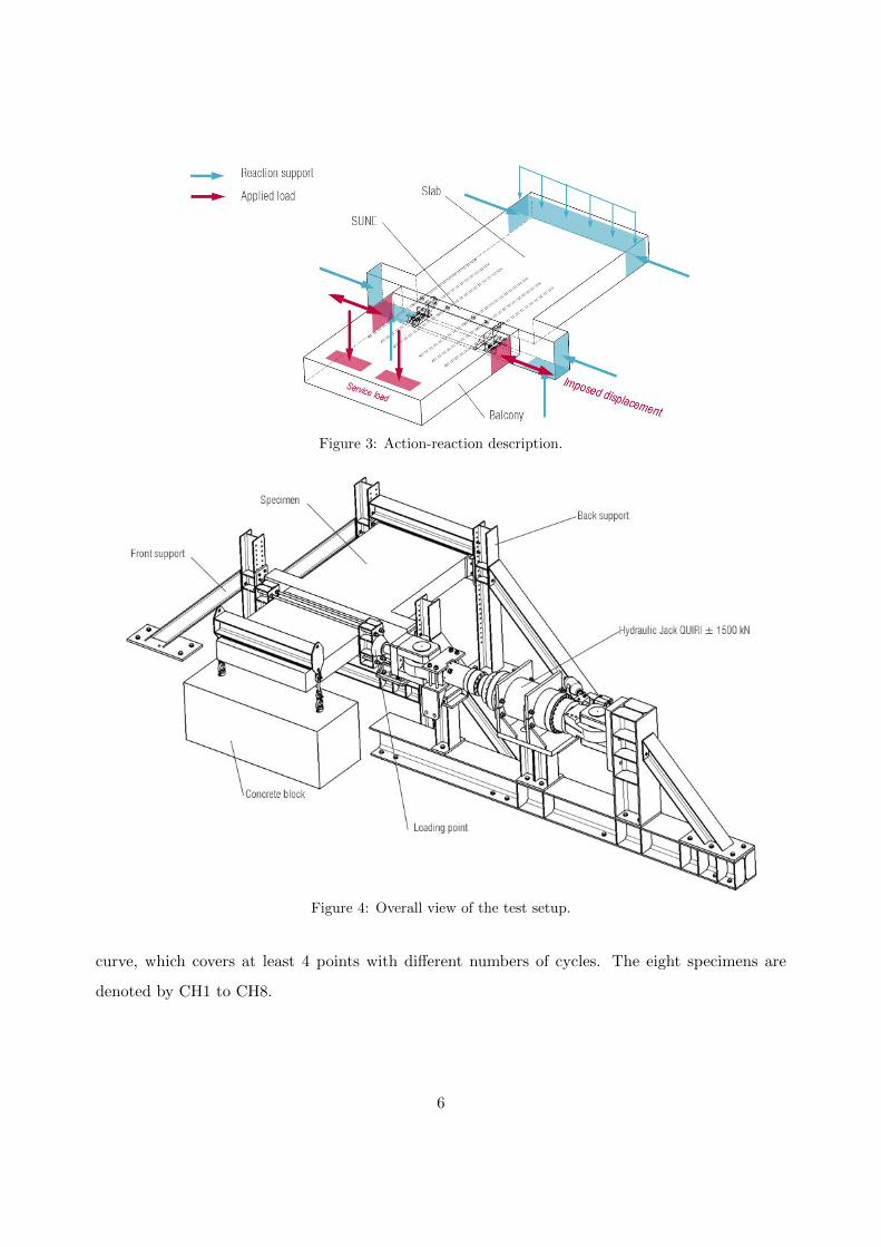
Figure 3: Action-reaction description.
Figure 4: Overall view of the test setup.
curve, which covers at least 4 points with different numbers of cycles. The eight specimens are
denoted by CH1 to CH8.
6

Figure 5: Detail of back and front supporting system.
Figure 6: Dimensions of the specimen in mm.
2.3. Materials
The concrete has a strength class of C25/30. The concrete characteristics at 28 days and at
the day of test are determined on cylinder samples with dimensions of 11 × 22 cm. 3 cylindric
concrete specimens are tested for each concrete age. The results of the compressive tests are listed
in Table 1.
2.4. Loading procedure
Cyclic tests are traditionally carried out with reference to Standard Procedures such as ECCS
[8] and ATC [9] which use loading histories consisting of groups of cycles at increasing amplitudes.
Such loading histories present the advantage of allowing on a single specimen a satisfactory appraisal
of the cyclic performance of the component. However, they appear inadequate for the development
7

Table 1: Mean material properties.
Specimen28 days day of test
fcm (MPa) Std. (MPa) fcm (MPa) Std. (MPa) Age (days)
CH1 36.49 0.14 34.91 0.51 39
CH2 25.97 0.37 29.85 0.51 71
CH3 32.46 0.11 31.94 0.47 43
CH4 27.60 0.58 32.77 0.20 37
CH5 27.60 0.58 28.56 0.52 50
CH6 29.35 0.60 30.80 0.84 35
CH7 29.35 0.60 30.13 0.36 43
CH8 31.28 0.20 35.45 0.50 48
of cumulative damage models useful not only for the seismic design of new structures but also
for the assessment of safety and reliability of damaged structures and for the development of
adequate repair procedures [10]. It has been recognised that repeating three cycles for each cycle
amplitude and then increasing the amplitude does not provide direct information regarding the
damage accumulation and strength degradation corresponding to one particular ductility demand;
in fact, increasing the amplitudes corresponds to an isotropic strain hardening effect resulting
in an increment of the load carrying capacity of the member, but this effect is opposite to the
strength degradation due to local failure and low-cycle fatigue, which are directly connected to the
cycle amplitude and the number of imposed cycles [11]. With regard to the recommended testing
procedure by ECCS, various researchers [10; 11] proposed a cyclic test with a constant amplitude
loading history in the plastic range. This proposal is complying with NF A03-403 [7] for low-cycle
fatigue tests to characterise the fatigue strength of the material.
For the present experimental tests, a sinusoidal form of the cycle is adopted, and the frequency
domain is between 0.03 Hz and 0.1 Hz. It is worth mentioning that at ambient temperature, the
frequency has generally less effect on the results of the tests [7]. At the beginning of the loading, 10
cycle loading is applied at an amplitude of 0.24 mm for CH1 and CH2 specimen; then, the loading
continues with increasing amplitude of 0.1 mm every 3 cycles up to an amplitude of 1.22 mm. The
latter amplitude is then maintained and the loading continues up to failure, see Fig. 7a. For other
8

specimens (CH3 to CH8), the loading is applied similarly. A 25 cycle loading with an amplitude
of 0.2 mm is employed at the beginning, followed by an amplitude increasing after every 3 cycles
with 0.1 mm increment until reaching the desired testing amplitude, see Fig. 7b. Every low-cycle
testing amplitude for each specimen is listed in Table 2.
-1.50
-1.00
-0.50
0.00
0.50
1.00
1.50
Dis
plac
emen
t (m
m)
Loading up to failure10 cycles Amplitude increases 0.1 mm after each 3 cycles
(a) CH1-CH2.
-3.00
-2.00
-1.00
0.00
1.00
2.00
3.00
Dis
plac
emen
t (m
m)
Loading up to failure25 cycles Amplitude increases 0.1 mm
after each 3 cycles
(b) CH3.
Figure 7: Loading history.
Table 2: Testing loading amplitude for each specimen.
Specimen CH1 CH2 CH3 CH4 CH5 CH6 CH7 CH8
Amplitude (mm) 1.22 1.22 2.44 1.83 1.52 1.52 2.75 5
9
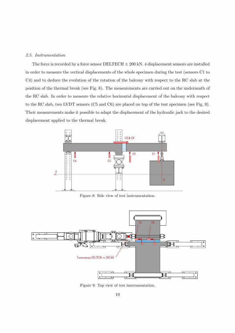
2.5. Instrumentation
The force is recorded by a force sensor DELTECH ± 200 kN. 4 displacement sensors are installed
in order to measure the vertical displacements of the whole specimen during the test (sensors C1 to
C4) and to deduce the evolution of the rotation of the balcony with respect to the RC slab at the
position of the thermal break (see Fig. 8). The measurements are carried out on the underneath of
the RC slab. In order to measure the relative horizontal displacement of the balcony with respect
to the RC slab, two LVDT sensors (C5 and C6) are placed on top of the test specimen (see Fig. 9).
Their measurements make it possible to adapt the displacement of the hydraulic jack to the desired
displacement applied to the thermal break.
Figure 8: Side view of test instrumentation.
Figure 9: Top view of test instrumentation.
10
2.6. Failure criterion
There are various methods to determine a failure criterion in fatigue. It is most commonly
associated with a test end criterion other than that of the total failure of the specimen. This
may depend on the interpretation of the results of the fatigue test and the nature of the device
tested. Most proposed failure criteria are based on the appearance, the presence or the worsening
of an observed phenomenon or recorded data, indicating extensive damage or a closely specimen
break. According to NF A03-403 [7] related to the testing of the resistance of metallic material
in low-cycle fatigue, the conventional number of cycles to failure can be defined as the number of
cycles corresponding to:
- the total failure of the test: separation into two distinct parts,
- a decrease of a certain percentage of the maximum tensile stress in relation to a given level thereof
during the test,
- a decrease of a certain percentage of the modulus of elasticity ratio in the tension part and the
compression part of the hysteresis loops,
- a decrease of a certain percentage of the maximum tensile stress in relation to the maximum
compressive stress.
Failure criteria are thus related to a decrease in resistance or stiffness. In the specific case of
the TBS, the level of resisting force is not a failure criterion, as the climatic action is an imposed
displacement. It is more logical to link the failure criterion to the loss of resistance of the TBS
under vertical action. As a consequence, the specimen will be considered as collapsed when a rapid
increase of the rotation of the TBS is observed.
Due to the fact that the value of the balcony rotation is not known during the tests but after
some mathematical operations using the measured values of the vertical displacement, the loading
is continued until the concrete block suspended to the balcony drops and reaches the floor. The
failure point can be then determined by evaluating the evolution of the balcony rotation. This
method can be referred to the third criteria described above, given the fact that the increase of
balcony deflection can be assimilated to a decrease of rotational stiffness.
11

2.7. Test results
This section presents the hysteretic cyclic response of the TBS, the failure modes and the
evolution of the jack force and the rotation of the balcony with the number of loading cycles. In
order to avoid any confusion, the number of cycles will be counted in half-sine cycles in the article.
2.7.1. Hysteretic cyclic response
In the following, we present the mechanical behaviour of the TBS under an incremental cyclic
loading. The force-displacement response of TBS under cyclic loading is depicted in Fig. 10 for
all specimens except CH2 and CH6 since the loading amplitude of those two are the same as CH1
and CH5, respectively. We can observe that the effect of concrete damaging is apparent in the
unloading branches through pinching.
−5 −4 −3 −2 −1 0 1 2 3 4 5−100
−50
0
50
100
Displacement (mm)
For
ce (
kN)
CH1
−5 −4 −3 −2 −1 0 1 2 3 4 5−100
−50
0
50
100
Displacement (mm)
For
ce (
kN)
CH3
−5 −4 −3 −2 −1 0 1 2 3 4 5−100
−50
0
50
100
Displacement (mm)
For
ce (
kN)
CH4
−5 −4 −3 −2 −1 0 1 2 3 4 5−100
−50
0
50
100
Displacement (mm)
For
ce (
kN)
CH5
−5 −4 −3 −2 −1 0 1 2 3 4 5−100
−50
0
50
100
Displacement (mm)
For
ce (
kN)
CH7
−5 −4 −3 −2 −1 0 1 2 3 4 5−100
−50
0
50
100
Displacement (mm)
For
ce (
kN)
CH8
Figure 10: Hysteretic cyclic response.
12

2.7.2. Failure modes
Even for the tests with the lowest amplitudes, the deformation of the U-shaped steel is visible
to the naked eye. A slight uplift of the end plates can even be observed. Nevertheless, this has
no impact on the fatigue strength of the thermal break.. The failure modes are similar for all
the specimens subjected to a small to moderate displacement amplitude (CH1 to CH7). They
are associated with the propagation cracks in U-shaped steel sections. The loading is continued
and the first cracks are observed at the first hundred of cycles on both U-shaped steel sections,
propagating diagonally from the hole at the end of the balcony-side slot towards the flanges of the
U-section. After continuing loading, other cracks are initiated in the welds or from the screws. At
the end, cracks propagate in the flanges. Consequently, the compression resistance of the thermal
break system drops significantly, resulting in an increasing balcony rotation until the concrete
block suspended to the balcony reaches the floor. These failure modes are categorized as type I
and type II in Table 3. The type III is observed only for the specimens CH7 and CH8, which have
been submitted to a very large loading amplitude. In this case, the collapse is guided by concrete
crushing.
The failure mode of each specimen is listed in Table 4. It is worth mentioning that the complete
failure of the specimen CH1 has not been attained during the test, i.e the loading has not been
continued until the concrete block, suspended to the balcony, drops and reaches the floor. The
loading has been stopped at 36000 half-cycles. However, at the last loading cycle, the force ampli-
tude had dropped by 22% and the rotation of the balcony had increased by 34% compared to the
values at the beginning of the test. As a result, the number of half-cycles of 36000 is considered as
the number of cycles that the specimen CH1 can sustain with the applied displacement amplitude
of 1.22 mm.
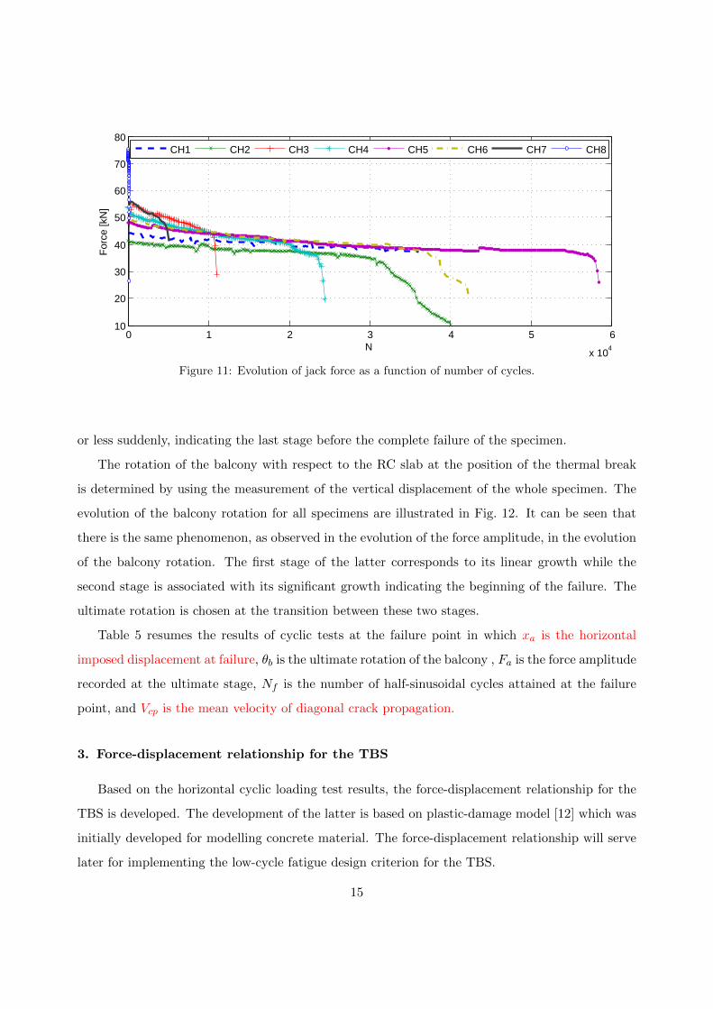
2.7.3. Evolution of jack force and balcony rotation
The jack force measurement using DELTECH ± 200 kN sensor is recorded regularly throughout
the test. The evolution of the force amplitude can be separated into two stages. A linear decrease
in the force amplitude per cycle is observed during the first stage of the test for all specimens, see
Fig. 11. At the second stage, the slope of the force amplitude-number of cycle curve drops more
13

Table 3: Failure mode description.
Mode Photo Description
Type (I)
Balcony
Lintel
The first cracks start near the hole at the end
of the balcony-side slot and propagate to the
flange of the U-shaped steel. The second cracks
initiate at the screw holes as well as in the welds.
These second cracks lead to a full fracture of the
U-shaped steel from the balcony.
Type (II)
Balcony
Lintel
The principal cracks initiate in the welds of the
U-shaped steel to the sub-plate embedded in
the lintel and grow up to full break-off. The
secondary cracks propagate diagonally from the
hole at the end of the balcony-side slot toward
the flanges of U-section.
Type (III)
Balcony
Lintel
The concrete crushing is observed on both sides
of the U-shaped steel.
Table 4: Failure mode of each specimen.
Specimen CH1 CH2 CH3 CH4 CH5 CG6 CH7 CH8
Failure mode (I) (I) (II) (I&II) (I&II) (I) (I&III) (III)
14
0 1 2 3 4 5 6
x 104
10
20
30
40
50
60
70
80
N
For
ce [k
N]
CH1 CH2 CH3 CH4 CH5 CH6 CH7 CH8
Figure 11: Evolution of jack force as a function of number of cycles.
or less suddenly, indicating the last stage before the complete failure of the specimen.
The rotation of the balcony with respect to the RC slab at the position of the thermal break
is determined by using the measurement of the vertical displacement of the whole specimen. The
evolution of the balcony rotation for all specimens are illustrated in Fig. 12. It can be seen that
there is the same phenomenon, as observed in the evolution of the force amplitude, in the evolution
of the balcony rotation. The first stage of the latter corresponds to its linear growth while the
second stage is associated with its significant growth indicating the beginning of the failure. The
ultimate rotation is chosen at the transition between these two stages.
Table 5 resumes the results of cyclic tests at the failure point in which xa is the horizontal
imposed displacement at failure, θb is the ultimate rotation of the balcony , Fa is the force amplitude
recorded at the ultimate stage, Nf is the number of half-sinusoidal cycles attained at the failure
point, and Vcp is the mean velocity of diagonal crack propagation.
3. Force-displacement relationship for the TBS
Based on the horizontal cyclic loading test results, the force-displacement relationship for the
TBS is developed. The development of the latter is based on plastic-damage model [12] which was
initially developed for modelling concrete material. The force-displacement relationship will serve
later for implementing the low-cycle fatigue design criterion for the TBS.
15

0 1 2 3 4 5 6
x 104
0.005
0.01
0.015
0.02
0.025
0.03
0.035
N
Rot
atio
n [r
ad]
CH1 CH2 CH3 CH4 CH5 CH6 CH7 CH8
Figure 12: Evolution of balcony rotation as a function of number of cycles.
Table 5: Results at assumed failure.
Specimen xa [mm] θb [rad] Fa [kN] Nf Vcp [mm/Nf ]
CH1 1.22 0.0139 37.844 36000 0.001232
CH2 1.22 0.0174 34.999 30000 0.001479
CH3 2.44 0.0229 46.961 8000 0.005612
CH4 1.83 0.0180 40.315 20000 0.002224
CH5 1.52 0.0255 38.027 54000 0.00082
CH6 1.52 0.0172 37.864 36000 0.001232
CH7 2.75 0.0295 47.251 4600 0.009876
CH8 5.00 0.0388 67.078 68 -
3.1. Force-displacement envelope curve
Assuming that the total horizontal displacement (x) can be decomposed into elastic (xe) and
plastic-damage (xpd) components, the generalised force (F ) versus generalised displacement (x)
can be described by the following equation:
x = xe + xpd =F
ke+
(F
k′
)1/n′
(1)
where ke is the elastic stiffness; k′ is the cyclic coefficient and n′ is the cyclic hardening exponent.
Eq. (1) is similar to the one proposed by Ramberg and Osgood [13] which is applied for true stress
and true strain relationship for ductile materials as stainless steel. Eq. (1) is totally empirical. The
16
parameter n′ is without unit. The coefficient k′ can be interpreted in logarithm scale of F and xpd.
Rewriting the relation of xpd and F in logarithm scale, we have:
logF = n′ log xpd + log k′ (2)
which means that k′ is equal to F when the plastic-damage displacement xpd is equal to unity. The
plastic-damage displacement xpd can be calculated by the following equation:
xpd = x− F
ke. (3)
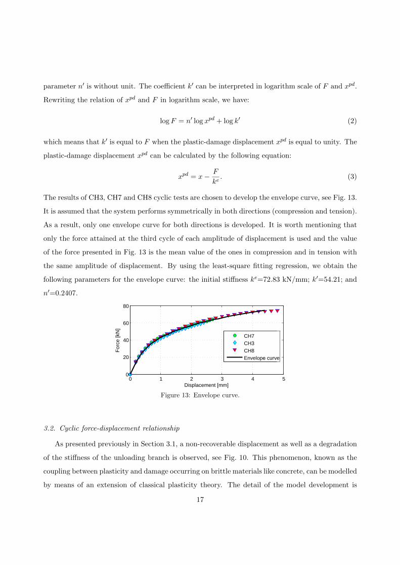
The results of CH3, CH7 and CH8 cyclic tests are chosen to develop the envelope curve, see Fig. 13.
It is assumed that the system performs symmetrically in both directions (compression and tension).
As a result, only one envelope curve for both directions is developed. It is worth mentioning that
only the force attained at the third cycle of each amplitude of displacement is used and the value
of the force presented in Fig. 13 is the mean value of the ones in compression and in tension with
the same amplitude of displacement. By using the least-square fitting regression, we obtain the
following parameters for the envelope curve: the initial stiffness ke=72.83 kN/mm; k′=54.21; and
n′=0.2407.
0 1 2 3 4 50
20
40
60
80
Displacement [mm]
For
ce [k
N]
CH7CH3CH8Envelope curve
Figure 13: Envelope curve.
3.2. Cyclic force-displacement relationship
As presented previously in Section 3.1, a non-recoverable displacement as well as a degradation
of the stiffness of the unloading branch is observed, see Fig. 10. This phenomenon, known as the
coupling between plasticity and damage occurring on brittle materials like concrete, can be modelled
by means of an extension of classical plasticity theory. The detail of the model development is
17
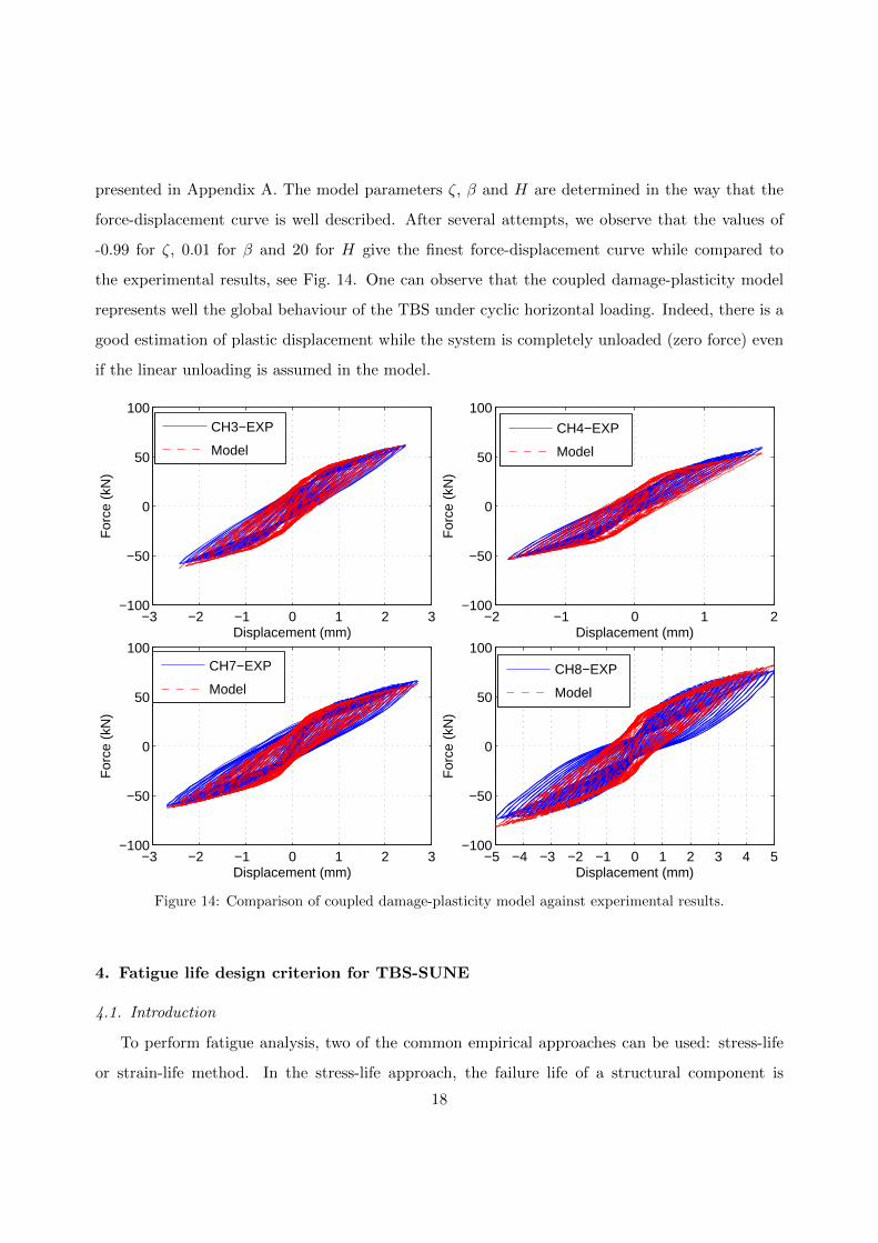
presented in Appendix A. The model parameters ζ, β and H are determined in the way that the
force-displacement curve is well described. After several attempts, we observe that the values of
-0.99 for ζ, 0.01 for β and 20 for H give the finest force-displacement curve while compared to
the experimental results, see Fig. 14. One can observe that the coupled damage-plasticity model
represents well the global behaviour of the TBS under cyclic horizontal loading. Indeed, there is a
good estimation of plastic displacement while the system is completely unloaded (zero force) even
if the linear unloading is assumed in the model.
−3 −2 −1 0 1 2 3−100
−50
0
50
100
Displacement (mm)
For
ce (
kN)
CH3−EXP
Model
−2 −1 0 1 2−100
−50
0
50
100
Displacement (mm)
For
ce (
kN)
CH4−EXP
Model
−3 −2 −1 0 1 2 3−100
−50
0
50
100
Displacement (mm)
For
ce (
kN)
CH7−EXP
Model
−5 −4 −3 −2 −1 0 1 2 3 4 5−100
−50
0
50
100
Displacement (mm)
For
ce (
kN)
CH8−EXP
Model
Figure 14: Comparison of coupled damage-plasticity model against experimental results.
4. Fatigue life design criterion for TBS-SUNE
4.1. Introduction
To perform fatigue analysis, two of the common empirical approaches can be used: stress-life
or strain-life method. In the stress-life approach, the failure life of a structural component is
18
estimated based upon the magnitude of the alternating stresses. One of the major drawbacks of
this approach is that it ignores the actual material response and treats all the behaviour as elastic.
This generally results in an overestimation of the fatigue life when the plastic strain contribution is
significant, particularly for the stainless steel. Thus, the stress-life method may not be applicable
when the plastic strain is not negligible, in low-cycle fatigue for example. Alternatively, the strain-
life approach estimates fatigue life using the total strain amplitude, including both the plastic and
elastic strain contributions. Thus, the strain-life methods can be applied in low-cycle fatigue where
significant plastic strains are present.
The relation between the fatigue life and elastic strain amplitude was first identified by Basquin
[14], who proposed a linear relationship between the logarithm of the stress amplitude and the
logarithm of fatigue life. The intercept at one stress reversal is defined as the fatigue strength
coefficient, σ′f , and is usually approximated by the true fracture strength of the metal. The fatigue
strength exponent (also known as Basquin’s exponent), b, is defined as the slope of the line. Thus,
the stress amplitude can be written as
σa = σ′f (Nf )b (4)
where σa is the stress amplitude and Nf is the fatigue life. The relationship between elastic strain
amplitude, εea, and fatigue life is then given as
εea =σaE
=σ′fE
(Nf )b (5)
where E is the modulus of elasticity. The relationship between fatigue life and the plastic strain
amplitude was independently identified by Coffin Jr [15] and Manson [16]. They found a linear
relation between the logarithm of the fatigue life and the logarithm of the stable plastic strain
amplitude, εpa, which can be written as
εpa = ε′f (Nf )c (6)
where ε′f is defined as the fatigue ductility coefficient and c is the fatigue ductility exponent which
is the slope of the line. In cyclic fatigue experiments, the fatigue ductility coefficient, ε′f , is usually
determined from the plastic strain intercept at one load reversal using the 0.2% offset yield strength
[17]. The strain-life method recognises that there is a transition from predominantly elastic effects
19

to predominantly plastic effects. Combining Eqs. (5) and (6) yields the so-called Manson-Coffin’s
strain-life equation:
εa = εea + εpa =σ′fE
(Nf )b + ε′f (Nf )c (7)
For a constant amplitude cyclic loading, Eq. (7) allows the number of cycles to failure to be
determined given the constant strain amplitude, εa, and the values of the material constants.
The material parameters can be obtained from monotonic and cyclic experiments. The strain
amplitude is obtained directly through strain measurement at critical locations or indirectly, either
analytically or approximately using finite element method.
From the perspective of applied cyclic stresses, fatigue damage of a component correlates
strongly with the applied stress amplitude. Experimental results indicate as well that the mean
stress influences very significantly on the total fatigue life [18]. In conjunction with the local strain
life approach, many models have been proposed to quantify the effect of mean stresses on fatigue
behaviour. The commonly used models in the ground vehicle industry are those by Morrow [19]
and by Smith et al. [20]. Morrow proposed the following relationship when a mean stress is present:
εa =σ′f − σm
E(Nf )b + ε′f (Nf )c (8)
In Eq. (8), the elastic part of the strain life curve is modified to take into account the mean normal
stress (σm). This model has been largely used in the long-life regime where plastic strain amplitude
is of less significance. Another model which is based on the energy description is proposed by
Smith et al. [20], so-called SWT model. It is assumed that the amount of fatigue damage in a
cycle is determined by the maximum energy produced in the component, which is the product of
the maximum tensile stress σmax and the strain amplitude εa. The SWT mean stress correction
formula is expressed as follows:
σmax εa =(σ′f )2
E(Nf )2b + σ′f ε
′f (Nf )b+c (9)
The SWT formula has been demonstrated to be successfully applied to several materials in the
range of low and high numbers of cycles by Boller and Seeger [21]. The SWT model is therefore
regarded as a more promising model for metallic materials.
20

4.2. Fatigue life prediction for TBS
Fatigue life criterions exposed above rely on local stresses and strains. This information may be
obtained in the present case by direct measurement or by local finite element analyses. However,
due to the geometry of the specimen, the direct measurement is very demanding. On the other
hand, the behaviour of the contact at the steel-concrete interface and of the concrete under the local
compression of the U profile, that have an important impact on these local stresses and strains,
are hardly represented in FE analyses. As a result, rather than entering in an uncertain complex
computation process, it has been decided to assess the TBS as a whole since it is usually adopted
for fatigue verifications in civil engineering.
Similar to SWT model, an energy-based fatigue criterion was proposed by Jahed and Varvani-
Farahani [22] to assess the fatigue lives of engineering components, which is expressed as:
∆Ef = E′e(Nf )B + E′f (Nf )C (10)
where ∆Ef is the energy due to the applied loading, E′f the fatigue toughness, E′e the strength
coefficient, C the toughness exponent and B is the fatigue strength exponent. Comparably to
Manson-Coffin’s equation, Eq. (10) is composed of elastic and plastic energy-life curve which cor-
responds to elastic and plastic energy contribution, respectively.
This approach can be used for TBS by forming the generalised force and displacement signal
following the force-displacement relationship described in Section 3. However, under variable-
amplitude cyclic loading, applying directly Eq. (10) may be not appropriate since the counting of
loading cycles may be inadequately performed. To overcome this shortcoming, the energy term is
replaced by the product of maximum absolute-generalised forces during loading cycle, Fmax and
the generalised displacement amplitude xa; Eq. (10) is then modified to
∆Emaxf = Fmax xa = E′e(Nf )B + E′f (Nf )C (11)
which is similar to SWT model. It should be noted that Fmaxxa is not the internal energy, but
an external work-like term. Since a low-cycle fatigue life of TBS is focused here, only the plastic
energy-life part of Eq. (11) is considered. Energy-fatigue life equation (Eq. (11)) is then reduced
to:
∆Emaxf = Fmax xa = E′f (Nf )C (12)
21
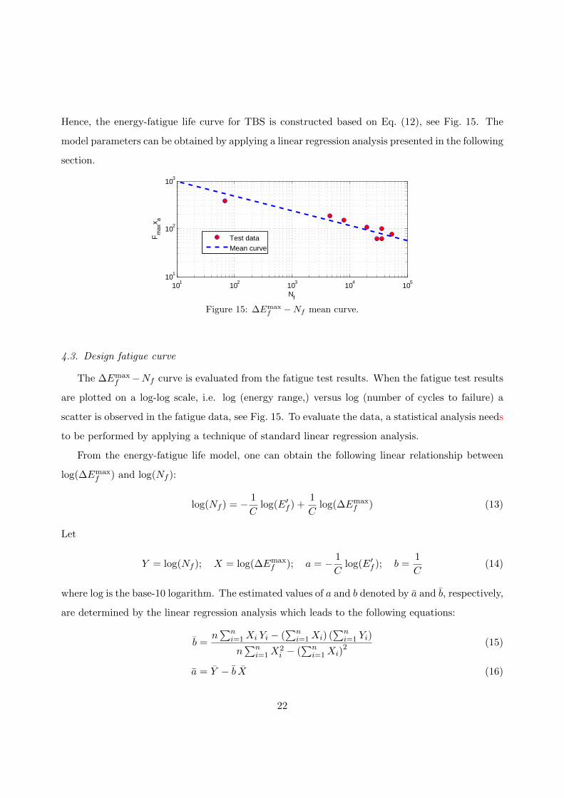
Hence, the energy-fatigue life curve for TBS is constructed based on Eq. (12), see Fig. 15. The
model parameters can be obtained by applying a linear regression analysis presented in the following
section.
101
102
103
104
105
101
102
103
Nf
Fm
axx a
Test dataMean curve
Figure 15: ∆Emaxf −Nf mean curve.
4.3. Design fatigue curve
The ∆Emaxf −Nf curve is evaluated from the fatigue test results. When the fatigue test results
are plotted on a log-log scale, i.e. log (energy range,) versus log (number of cycles to failure) a
scatter is observed in the fatigue data, see Fig. 15. To evaluate the data, a statistical analysis needs
to be performed by applying a technique of standard linear regression analysis.
From the energy-fatigue life model, one can obtain the following linear relationship between
log(∆Emaxf ) and log(Nf ):
log(Nf ) = − 1
Clog(E′f ) +
1
Clog(∆Emax
f ) (13)
Let
Y = log(Nf ); X = log(∆Emaxf ); a = − 1
Clog(E′f ); b =
1
C(14)
where log is the base-10 logarithm. The estimated values of a and b denoted by a and b, respectively,
are determined by the linear regression analysis which leads to the following equations:
b =n∑n
i=1Xi Yi − (∑n
i=1Xi) (∑n
i=1 Yi)
n∑n
i=1X2i − (
∑ni=1Xi)
2 (15)
a = Y − b X (16)
22
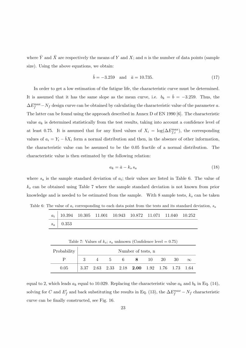
where Y and X are respectively the means of Y and X; and n is the number of data points (sample
size). Using the above equations, we obtain:
b = −3.259 and a = 10.735. (17)
In order to get a low estimation of the fatigue life, the characteristic curve must be determined.
It is assumed that it has the same slope as the mean curve, i.e. bk = b = −3.259. Thus, the
∆Emaxf −Nf design curve can be obtained by calculating the characteristic value of the parameter a.
The latter can be found using the approach described in Annex D of EN 1990 [6]. The characteristic
value ak is determined statistically from the test results, taking into account a confidence level of
at least 0.75. It is assumed that for any fixed values of Xi = log(∆Emaxf,i ), the corresponding
values of ai = Yi − bXi form a normal distribution and then, in the absence of other information,
the characteristic value can be assumed to be the 0.05 fractile of a normal distribution. The
characteristic value is then estimated by the following relation:
ak = a− ks sa (18)
where sa is the sample standard deviation of ai; their values are listed in Table 6. The value of
ks can be obtained using Table 7 where the sample standard deviation is not known from prior
knowledge and is needed to be estimated from the sample. With 8 sample tests, ks can be taken
Table 6: The value of ai corresponding to each data point from the tests and its standard deviation, sa
ai 10.394 10.305 11.001 10.943 10.872 11.071 11.040 10.252
sa 0.353
Table 7: Values of ks; sa unknown (Confidence level = 0.75)
Probability Number of tests, n
P 3 4 5 6 8 10 20 30 ∞
0.05 3.37 2.63 2.33 2.18 2.00 1.92 1.76 1.73 1.64
equal to 2, which leads ak equal to 10.029. Replacing the characteristic value ak and bk in Eq. (14),
solving for C and E′f and back substituting the results in Eq. (13), the ∆Emaxf −Nf characteristic
curve can be finally constructed, see Fig. 16.
23
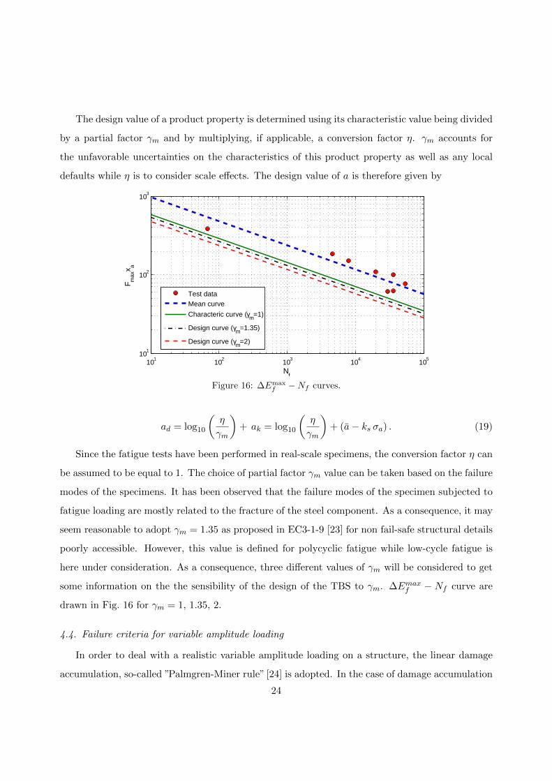
The design value of a product property is determined using its characteristic value being divided
by a partial factor γm and by multiplying, if applicable, a conversion factor η. γm accounts for
the unfavorable uncertainties on the characteristics of this product property as well as any local
defaults while η is to consider scale effects. The design value of a is therefore given by
101
102
103
104
105
101
102
103
Nf
F max
x a
Test dataMean curve
Characteric curve (γm=1)
Design curve (γm=1.35)
Design curve (γm=2)
Figure 16: ∆Emaxf −Nf curves.
ad = log10
(η
γm
)+ ak = log10
(η
γm
)+ (a− ks σa) . (19)
Since the fatigue tests have been performed in real-scale specimens, the conversion factor η can
be assumed to be equal to 1. The choice of partial factor γm value can be taken based on the failure
modes of the specimens. It has been observed that the failure modes of the specimen subjected to
fatigue loading are mostly related to the fracture of the steel component. As a consequence, it may
seem reasonable to adopt γm = 1.35 as proposed in EC3-1-9 [23] for non fail-safe structural details
poorly accessible. However, this value is defined for polycyclic fatigue while low-cycle fatigue is
here under consideration. As a consequence, three different values of γm will be considered to get
some information on the the sensibility of the design of the TBS to γm. ∆Emaxf − Nf curve are
drawn in Fig. 16 for γm = 1, 1.35, 2.
4.4. Failure criteria for variable amplitude loading
In order to deal with a realistic variable amplitude loading on a structure, the linear damage
accumulation, so-called ”Palmgren-Miner rule” [24] is adopted. In the case of damage accumulation
24
methods in combination with ∆Emaxf −Nf curve, the verification rule can be presented as
∑ nE,i
Nf,i<Dc
γd(20)
where
- nE,i is the number of applied load cycles with the loading range level obtained from the rainflow
counting procedure;
- Nf,i is the number of load cycles at failure for loading range level taking into account the uncer-
tainties in the structural resistance;
- Dc is the critical value for the damage ratio, in the ideal case taken equal to 1;
- γd is the partial factor that deals with the uncertainties in damage accumulation rule, the design
working life and the consequences of failure. Its value is assumed to be equal to 1.
5. Thermal action
As mentioned in Section 1, the balcony suffers climatic hazards and is caused to expand or
shorten following the variation of the temperature outside the building. The deformation of the
balcony produces then a shear force on the thermal break system. To determine the action effects
on the latter, the variation of the temperature has to be known. The procedure to define the
temperature data and to obtain the displacement applied to the thermal break system is presented
in this section.
5.1. ECA&D temperature database
European Climate Assessment & Dataset (ECA&D) [25] was initiated by the ECSN in 1998
and has received financial support from the EUMETNET and the European Commission. ECA&D
forms the backbone of the climate data node in the Regional Climate Centre (RCC) for WMO
Region VI (Europe and the Middle East) since 2010. The data and information products contribute
to the Global Framework for Climate Services (GFCS). Today, ECA&D is receiving data from 68
participants for 63 countries and the ECA data set contains 43271 series of observations for 12
elements at 10586 meteorological stations throughout Europe and the Mediterranean zone.
25

5.2. Factorised temperature distribution
From the ECA&D website, we can have the data of the temperature for certain meteorological
stations in Europe, particularly in France. The maximum and minimum temperature distribution
over the years obtained from ECA&D database is compared to the distribution of extreme value
given by EN 1991-1-5 [26]. Indeed, the maximum (minimum) shade air temperature Tmax (Tmin)
given by EN 1991-1-5 is supposed to be the value of maximum (minimum) shade air temperature
with an annual probability of being exceeded of 0.02 (equivalent to a mean return period of 50
years), based on the maximum (minimum) hourly values recorded. EN 1991-1-5 provides the
following expressions based on extreme value distributions of type-I to determine the maximum (or
minimum) temperature of the shade air, Tmax,p (Tmin,p) based on an annual probability of being
exceeded p different from 0.02:
Tmax,p = Tmax {k1 − k2 ln [− ln(1− p)]} (21)
Tmin,p = Tmin {k3 + k4 ln [− ln(1− p)]} (22)
where k1, k2, k3 and k4 can be taken equal to 0.781, 0.056, 0.393, -0.156, respectively.
The comparisons of maximum and minimum annual shade air temperature distribution obtained
from several meteorological stations (ECA&D) and the one given by the default values of EN 1991-
1-5 are illustrated in Fig. 17, where the maximum and minimum shade air temperature (Tmax,
Tmin) are obtained from National Annex (NF EN 1991-1-5/NA). It can be seen from Fig. 17 that
there is a large dispersion between the shade air temperature distributions obtained from ECA&D
and the Eurocode one. The Eurocode default curve of the maximum annual shade air temperature
distribution does not fit satisfactorily to any meteorological stations while the minimum annual
shade air temperature distribution of Eurocode fits satisfactorily to Rennes station which is at the
north-west of France.
The value of maximum shade air temperature obtained from ECA&D with an annual probability
of being exceeded of 0.02 does not correspond to the one given by NF EN 1991-1-5/NA. It can
be seen that for certain meteorological stations, Rennes for instance, the ratio Tmax,p/Tmax is
significantly greater than 1. However, it is only one of the cases studied and most of these ratios
are lesser than 1 for other stations. We assume that Tmax and Tmin given by NF EN 1991-1-5/NA
are the values that must be considered for design. As a consequence, the signal of temperature
26

0 0.2 0.4 0.6 0.8 10
0.1
0.2
0.3
0.4
0.5
0.6
0.7
0.8
0.9
1
1.1
1.2
Cumulative probability (p)
Tm
in,p
/ T m
in
ParisRennesStrasbourgBordeauxEmbrunEN1991−1−5 (defaut)
(a) Distribution of minimum annual temperature.
0 0.2 0.4 0.6 0.8 10.5
0.6
0.7
0.8
0.9
1
1.1
1.2
Cumulative probability (p)
Tm
ax,p
/ T m
ax
ParisRennesStrasbourgBordeauxEmbrunEN1991−1−5 (defaut)
(b) Distribution of maximum annual temperature.
Figure 17: Distribution of annual temperature.
obtained from ECA&D with Tmax,0.02 or Tmin,0.02 lesser than Tmax or Tmin given by NF EN 1991-
1-5/NA must be adopted. To do so, the following linear expansion formulation of the signal is
adopted:
T (t) = T0(t)
[Tmax
Tmax,0.02+
(Tmin
Tmin,0.02− Tmax
Tmax,0.02
)(Tmax,0.02 − T0(t)
Tmax,0.02 − Tmin,0.02
)](23)
where
- T0(t) is the temperature of the initial signal (ECA&D);
- Tmax,0.02 is the maximum temperature of the initial signal with an annual probability of being
exceeded of 0.02;
- Tmin,0.02 is the minimum temperature of the initial signal with an annual probability of being
exceeded of 0.02;
- Tmax is the maximum temperature from NF EN 1991-1-5/NA with an annual probability of
being exceeded of 0.02;
- Tmin is the minimum temperature from NF EN 1991-1-5/NA with an annual probability of being
exceeded of 0.02.
The factorization is performed only when Tmax,0.02 is less than Tmax or when Tmin,0.02 is greater than
Tmin. The temperature distribution after factorizing is shown in Fig. 18. It can be seen that while
calibrating Tmin,0.02 and Tmax,0.02 of the initial signal to Tmin and Tmax of NF EN 1991-1-5/NA,
27

respectively, the factorized maximum as well as minimum temperature with cumulative probability
p greater than 0.02 alter to be larger in absolute value. This reshapes the temperature distribution,
particularly for maximum temperature, and leads to a wide scatter compared to the ones given by
NF EN 1991-1-5.
0 0.2 0.4 0.6 0.8 10
0.1
0.2
0.3
0.4
0.5
0.6
0.7
0.8
0.9
1
1.1
1.2
Cumulative probability (p)
Tm
in,p
/ T m
in
ParisRennesStrasbourgBordeauxEmbrunEN1991−1−5 (defaut)
(a) Factorized distribution of minimum annual tem-
perature.
0 0.2 0.4 0.6 0.8 10.5
0.6
0.7
0.8
0.9
1
1.1
1.2
Cumulative probability (p)
Tm
ax,p
/ T m
ax
ParisRennesStrasbourgBordeauxEmbrunEN1991−1−5 (defaut)
(b) Factorized distribution of maximum annual tem-
perature.
Figure 18: Factorized distribution of annual temperature.
5.3. Solar radiation
Solar radiation has important effects in generating heat on the surface of the balcony. For
buildings above the ground level, the following values in Table 8 [26] are adopted for solar radi-
ation effects. To be conservative, the dark colored surface is considered. Consequently, there is
Table 8: Indicative temperature Toutfor buildings above the ground level.
Season Significant factor Temperature Tout in ◦C
Summer
Relative absorptivity 0.5 Bright light surface Tmax + T3
depending on surface color 0.7 Light colored surface Tmax + T4
0.9 Dark surface Tmax + T5
Winter Tmin
Note: T3 = −10 ◦C; T4 = 0 ◦C; T5 = 10 ◦C given by NF EN 1991-1-5/NA.
a modification on the signal of temperature due to solar radiation effects by adding T5 to Tmax
28
defined by the national annex. The daily design temperature (Eq. (23)) is then modified to:
T (t) = T0(t)
[Tmax + T5Tmax,0.02
+
(Tmin
Tmin,0.02− Tmax + T5
Tmax,0.02
)(Tmax,0.02 − T0(t)
Tmax,0.02 − Tmin,0.02
)](24)
5.4. Conversion of temperature signal to displacement signal
From the design temperature obtained by using Eq. (24), we calculate the variation of outdoor-
indoor temperature ∆T with respect to time. It is here assumed that the temperature inside the
building varies during the year, see Table 9, as estimated by NF EN 1991-1-5 [26]. The horizontal
axial deformation of the balcony, supposed to be symmetric from the central axis of the balcony, is
then determined from the variation of outdoor-indoor temperature in association with the balcony
length, Lb. This deformation will generate the horizontal displacement imposed to TBS-SUNE at
both extremities of the balcony.
Table 9: Temperature inside the building Tinside in ◦C
Date Tinside
22 March - 21 June 22.5
22 June - 21 September 20.0
22 September - 21 December 22.5
22 December - 21 March 25.0
The corresponding displacement is given by:
x = α∆TLb
2(25)
where α = 10−5 is the coefficient of thermal dilatation of concrete and ∆T = T (t)− Tinside(t).
6. Verification to thermal loading
6.1. Steps of the method and general assumptions
The verification of TBS against thermal loading can be performed by determining the damage
accumulation developed during the building life. This can be done for an existing building where
the distribution of temperature is already known. To design a new building where the climate
surrounding the building is not yet known during the building life, a probabilistic approach has to
be developed.
29

It is assumed that the statistical distribution of the climatic action can be computed on the basis
of the distribution of the recordings of ECA & D, transformed as explained in previous paragraphs
in order to get thermal amplitudes compliant with actual European standards.
The climatic action in fatigue is defined on the basis of a duration of one year, from 22nd of
March to 21st of March, i.e. from spring to spring. The annual accumulated damage Dy of the
year i is then obtained from:
Dy,i =
m∑j=1
nE,j
Nf,j(26)
where m is the number of different displacement amplitudes xa,j obtained from rainflow counting
technique; nE,j is the number of semi-sinusoidal cycle of each rainflow displacement amplitude
xa,j ; and Nf,j is the number of semi-sinusoidal cycle to failure obtained from ∆Emaxf −Nf design
curve for each rainflow displacement amplitude xa,j . In order to use ∆Emaxf −Nf design curve, the
maximum absolute-generalised forces during loading cycle, Fmax, is required. The analysis with the
annual displacement signal is then primarily performed to capture the corresponding force signal
acting on the structure by using the coupled damage-plasticity model developed in this paper.
It is worth noting that the rainflow counting algorithm developed by Nies lony [27] is used. This
algorithm also provides the start and end point of the loading cycle which can be used to determine
the index of the loading cycle, and as a result the value of Fmax for each rainflow displacement
amplitude xa,j .
Processing all the data of ECAD for one station gives a set of values of Dy,i that is used to
obtain an estimation of the mean value µDy and of the standard deviation σDy .
The service life is fixed to 50 years in Eurocodes for usual buildings, and the related accumulated
damage denoted D50 has to be limited to 1. D50 is a random variable equal to the sum of 50 annual
damages. Each annual damage is supposed to be independent. Hence, according to the central limit
theorem, the data set of D50, which is a sum of independent random variables, follows a normal
distribution N (50 µDy , 50 σ2Dy) even if Dy,i is not normally distributed. Within a data sample size
equal to nyear, the characteristic value of D50 can be obtained using the following expression:
D50,k = 50 µDy + tv√
50 σDy (27)
It is worth mentioning that the available data signal from ECA&D is usually greater than 50
years and that the value of tv is determined by using the inverse value of Student’s cumulative
30
distribution function, multiplied by√
1 + 1/nyear.
Since the ∆Emaxf −Nf design curve is used to determine the damage parameter, the character-
istic value D50,k can be then considered as design value D50,d.
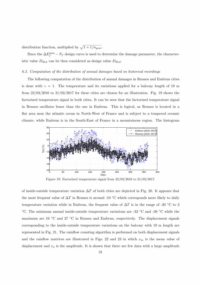
6.2. Computation of the distribution of annual damages based on historical recordings
The following computation of the distribution of annual damages in Rennes and Embrun cities
is done with γ = 1. The temperature and its variations applied for a balcony length of 19 m
from 22/03/2016 to 21/03/2017 for these cities are chosen for an illustration. Fig. 19 shows the
factorized temperature signal in both cities. It can be seen that the factorized temperature signal
in Rennes oscillates lesser than the one in Embrun. This is logical, as Rennes is located in a
flat area near the atlantic ocean in North-West of France and is subject to a tempered oceanic
climate, while Embrun is in the South-East of France in a mountainous region. The histogram
0 50 100 150 200 250 300 350 400−40
−30
−20
−10
0
10
20
30
Days
T(t
) (°
C)
Embrun (2016−2017)Rennes (2016−2017)
Figure 19: Factorized temperature signal from 22/03/2016 to 21/03/2017.
of inside-outside temperature variation ∆T of both cities are depicted in Fig. 20. It appears that
the most frequent value of ∆T in Rennes is around -10 ◦C which corresponds more likely to daily
temperature variation while in Embrun, the frequent value of ∆T is in the range of -20 ◦C to 3
◦C. The minimum annual inside-outside temperature variations are -33 ◦C and -38 ◦C while the
maximum are 16 ◦C and 27 ◦C in Rennes and Embrun, respectively. The displacement signals
corresponding to the inside-outside temperature variations on the balcony with 19 m length are
represented in Fig. 21. The rainflow counting algorithm is performed on both displacement signals
and the rainflow matrices are illustrated in Figs. 22 and 23 in which xm is the mean value of
displacement and xa is the amplitude. It is shown that there are few data with a large amplitude
31

−40 −30 −20 −10 0 10 20 300
10
20
30
40
50
60
70
∆T (°C)
N. o
ccur
ence
s
Rennes (2016−2017)Embrun (2016−2017)
Figure 20: Histogram of inside-outside temperature variation from 22/03/2016 to 21/03/2017.
in the rainflow matrix. Those few data correspond to the annual temperature variations. The
large density of rainflow matrix are condensed in the low amplitude range which is more or less
related to the daily temperature variation. Besides, a large number of displacement amplitude in
the rainflow matrix are larger than 0.5 mm, the displacement amplitude which can induce yielding
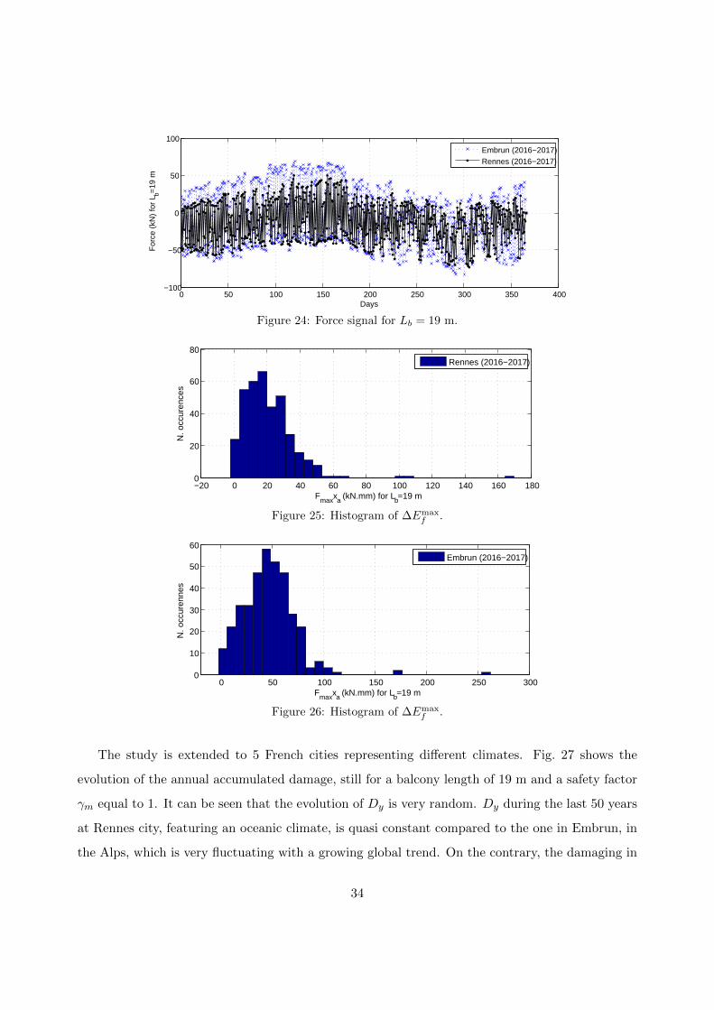
of the thermal break system, see Fig. 13. The force signals, see Fig. 24 in response to the
0 50 100 150 200 250 300 350 400−4
−3
−2
−1
0
1
2
3
Days
x (m
m)
for
L b=19
m
Embrun (2016−2017)Rennes (2016−2017)
Figure 21: Displacement signal for Lb = 19 m.
displacement signals, are obtained by performing the analyses using the coupled damage-plasticity
model. From the force signal, the absolute value of maximum force Fmax during the the rainflow
loading cycle can be obtained. The histogram of ∆Emaxf = Fmaxxa for each city can be constructed,
see Figs. 25 and 26. It is clear that the value and frequency of ∆Emaxf developed on the thermal
32

0.5 1 1.5 2
−2.5
−2
−1.5
−1
−0.5
0
0.5
rainflow matrix
xa
x m
Num
ber
of c
ycle
s
1
2
3
4
5
6
7
8
Figure 22: Rainflow matrix of displacement signal in Rennes.
0.5 1 1.5 2 2.5 3
−2.5
−2
−1.5
−1
−0.5
0
0.5
1
Num
ber
of c
ycle
s
xa
rainflow matrix
x m
1
2
3
4
5
6
7
8
Figure 23: Rainflow matrix of displacement signal in Embrun.
break system while being used in the buildings in Embrun is larger than the one in Rennes. As a
result, the annual accumulated damage in Embrun is larger than the one in Rennes.
33
0 50 100 150 200 250 300 350 400−100
−50
0
50
100
Days
For
ce (
kN)
for
L b=19
m
Embrun (2016−2017)Rennes (2016−2017)
Figure 24: Force signal for Lb = 19 m.
−20 0 20 40 60 80 100 120 140 160 1800
20
40
60
80
Fmaxxa (kN.mm) for Lb=19 m
N. o
ccur
ence
s
Rennes (2016−2017)
Figure 25: Histogram of ∆Emaxf .
0 50 100 150 200 250 3000
10
20
30
40
50
60
Fmaxxa (kN.mm) for Lb=19 m
N. o
ccur
enne
s
Embrun (2016−2017)
Figure 26: Histogram of ∆Emaxf .
The study is extended to 5 French cities representing different climates. Fig. 27 shows the
evolution of the annual accumulated damage, still for a balcony length of 19 m and a safety factor
γm equal to 1. It can be seen that the evolution of Dy is very random. Dy during the last 50 years
at Rennes city, featuring an oceanic climate, is quasi constant compared to the one in Embrun, in
the Alps, which is very fluctuating with a growing global trend. On the contrary, the damaging in
34
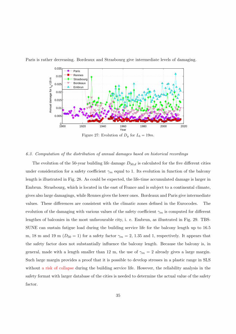
Paris is rather decreasing. Bordeaux and Strasbourg give intermediate levels of damaging.
1900 1920 1940 1960 1980 2000 20200
0.005
0.01
0.015
0.02
0.025
0.03
0.035
Year
Ann
ual d
amag
e fo
r L b=
19 m
ParisRennesStrasbourgBordeauxEmbrun
Figure 27: Evolution of Dy for Lb = 19m.
6.3. Computation of the distribution of annual damages based on historical recordings
The evolution of the 50-year building life damage D50,d is calculated for the five different cities
under consideration for a safety coefficient γm equal to 1. Its evolution in function of the balcony
length is illustrated in Fig. 28. As could be expected, the life-time accumulated damage is larger in
Embrun. Strasbourg, which is located in the east of France and is subject to a continental climate,
gives also large damagings, while Rennes gives the lower ones. Bordeaux and Paris give intermediate
values. These differences are consistent with the climatic zones defined in the Eurocodes. The
evolution of the damaging with various values of the safety coefficient γm is computed for different
lengthes of balconies in the most unfavourable city, i. e. Embrun, as illustrated in Fig. 29. TBS-
SUNE can sustain fatigue load during the building service life for the balcony length up to 16.5
m, 18 m and 19 m (D50 = 1) for a safety factor γm = 2, 1.35 and 1, respectively. It appears that
the safety factor does not substantially influence the balcony length. Because the balcony is, in
general, made with a length smaller than 12 m, the use of γm = 2 already gives a large margin.
Such large margin provides a proof that it is possible to develop stresses in a plastic range in SLS
without a risk of collapse during the building service life. However, the reliability analysis in the
safety format with larger database of the cities is needed to determine the actual value of the safety
factor.
35

0 5 10 15 20 250
0.5
1
1.5
2
2.5
3
3.5
4
4.5
Length of balcony in m
D50
,d
ParisRennesStrasbourgBordeauxEmbrun
Figure 28: Evolution of D50,d in function of Lb with γm = 1
.
0 5 10 15 20 250
1
2
3
4
5
6
7
8
9
Length of balcony in m
D50
,d
Embrun city
γm
=2
γm
=1.35
γm
=1
Figure 29: Evolution of D50,d in function of Lb in Embrun city with different values of γm.
7. Conclusions and perspectives
The procedure for verifying the thermal break system SUNE against low-cycle fatigue loads
induced by the deformations of the balcony due to the variations of the temperature has been
presented in this paper. Primarily, eight cyclic experimental tests of the system are performed
with several loading amplitudes. On one hand, they serve to define the fatigue design curve. On
the other hand, they allow to develop a coupled plastic-damage mechanical model of the device.
36
Then, the past temperature variations taken from ECA & D database for five different cities are
scaled in order to comply with the extreme values recommended in the Eurocodes. After adding
the effect of the solar radiations, the elongation histories are computed for different lengthes of
balconies. Force-displacement histories are deduced using the mechanical model, and the cycles
applied to the system are counted by a rainflow algorithm. Finally, the fatigue design curve allows
to verify the fatigue strength of the thermal break for the different configurations considered. The
process is applied in five different cities for different lengths of balconies.
As could be expected, the annual accumulated damage is larger in mountainous regions than
in tempered areas, and the evolution of the damage follows the same trends as the minimum and
the maximum shade air temperatures defined in the French national annex of the Eurocode.
The design format and the related safety coefficients are not known at this stage. But, it is clear
that a safe design can be achieved for usual lengths of balconies at least up to 12 m. Moreover, a
parametric study shows that the maximum length of the balcony is not proportional to the safety
coefficient and that, even with a safety coefficient of 2, a balcony length of 16 m can be reached in
the most unfavourable location considered in the study.
This specific case illustrates that it is possible to exceed the conventional 0.2 percents yielding
during service life without any risk for the integrity of the components. This offers a wide range
of new possibilities, particularly in the case of shear keys used in thermal break systems.
Further investigations through reliability analysis are however needed in order to define an
accurate safety format.
8. Acknowledgements
The authors gratefully acknowledge financial support by the ANR (Agence Nationale de la
Recherche, France) through the project LabCom ANR B-HYBRID.
Appendix A Cyclic force-displacement relationship
A.1 Yield function for TBS
By taking into account the isotropic and kinematic hardening, the yield function for TBS-SUNE
system is proposed as follow:
f (F, F q, R) = |F − F q| −R (A-1)
37
where F q and R are the thermodynamic force associated to the kinematic and isotropic hardening,
respectively.
A.2 Coupled plastic-damage model
The following model is presented initially by Meschke et al. [12]. It is herein presented for one
dimensional case in which forces and displacements are considered as variables.
The following set of state variables is assumed for the thermodynamic state at any time t:
{xe, xp, xd, p, q} (A-2)
where x is total displacement, xp plastic displacement, xd displacement associated to damage, p the
internal variable associated with the isotropic hardening and q is the internal variable associated to
the kinematic hardening. The choice of the internal variables is not unique. In fact, it is possible
to substitute the displacement associated to damage by the plastic displacement. To do so, it is
sufficient to observe that:
F = ke xe = kd xd = k (x− xp) (A-3)
in which ke is elastic moduli and kd is damage moduli that varies in function of the non-recoverable
displacement. Following the above hypothesis, the total work done by the force F is assumed to
have the form:
W = W(xe, xp, Dd, p, q
)(A-4)
in which Dd = 1/kd is the damage compliance moduli. It is usual to assume that the total work
can be split as
W = W e(xe) +W d(xd, Dd) +W p(p) +W q(q) (A-5)
where
- W e(xe) =1
2xe ke xe is the work corresponding to the elastic displacement, see Fig. A1; and
- W d(xd, Dd) =1
2xd kd xd is the work corresponding to the displacement associated to damage
which can be rewritten as W d(xd, Dd) =1
2xd kd xd = xd kd xd − 1
2xd kd xd = F xd − 1
2Dd F 2.
38

F
x
xe
xexdxp
x
kek
kd
ke
1
2d d d d dW x x k x
1
2e e e e eW x x k x
Figure A1: Elasto-plastic damage model.
Inserting the expressions of W e(xe) and W d(xd, Dd) in to Eq. (A-5) and making use of Eq. (A-3),
we can rewrite the expression of the total work as follow:
W = W ed(x, xp, Dd) +W p(p) +W q(q) (A-6)
where W ed(x, xp, Dd) =1
2
(De +Dd
)−1(x− xp)2 =
1
2D−1 (x− xp)2 , De = 1/ke and D = 1/k .
The Clausius-Duhem inequality requires
0 ≤ D = F x− W (A-7)
Substituting Eq. (A-6) into Eq. (A-7), and making partial differential operation on each part of
total work, one has:
D =
(F − ∂W ed
∂(x− xp)
)x+
∂W ed
∂(x− xp)xp − ∂W ed
∂DdDd − ∂W p
∂pp− ∂W q
∂qq (A-8)
Eq. (A-8) must be satisfied for all evolutions containing the elastic case without damage where
xp = 0, Dd = 0, p = 0 and q = 0; this implies the first elastic state law:
F =∂W ed
∂(x− xp)= D−1(x− xp) (A-9)
39

From Eq. (A-9), we define the following thermodynamic forces:
Y =∂W ed
∂Dd= −1
2F 2 (A-10)
R(p) =∂W p
∂p(A-11)
F q(q) =∂W q
∂q(A-12)
The Clausius-Duhem inequality is then reduced to
D = F xp +1
2F 2 Dd −R(p) p− F q(q) q ≥ 0 (A-13)
The interest here is to introduce a coupling between the two phenomena by introducing a single
criterion that depends only on F , R(p) and F q(q). In the absence of an explicit criterion on Y ,
one can overcome its presence in the dissipation inequality. The area of convex reversibility C is
defined in the space of thermodynamic forces (F, F q, R). It can be written as
C := {(F, F q, R) | f(F, F q, R) ≤ 0} (A-14)
where the yield surface f(F, F q, R) = 0 limits this area; inside which, no irreversibility is possible.
In analogy to classical plasticity theory, the evolution of the compliance moduli Dd, of the in-
elastic displacement xp and of the internal variables (p, q) is obtained from exploiting the postulate
of maximum dissipation [28].
inf(F, F q , R)
[−D
](A-15)
Thus, for a given set of variables in the admissible state (F, F q, R) ∈ C, the rates(xp, Dd, p and q
)are those that produce a stationary point of dissipation D. To find the solution of this problem,
the Lagrange multiplier method is used. The following Lagrangean function is introduced
L(F, F q, R) = −D + λ f(F, F q, R) (A-16)
= F xp +1
2F 2 Dd −R(p) p− F q(q) q + λ f(F, F q, R) (A-17)
where λ ≥ 0 is Lagrange multiplier. From the associated optimality conditions:
∂L
∂F= 0;
∂L
∂F q= 0;
∂L
∂R= 0, (A-18)
40

one gets:
xp + Dd F = λ∂f
∂F(A-19)
q = −λ ∂f
∂F q(A-20)
p = −λ ∂f∂R
(A-21)
Defining the differential displacement associated with the degradation of the compliance moduli by
xda = Dd F (A-22)
and the inelastic displacement rate by
xpd = xp + xda, (A-23)
one can rewrite Eq. (A-19) in the form analogous to classical associative plasticity theory as
xpd = λ∂f
∂F(A-24)
It can be observed that the inelastic displacement rate xpd is composed of two parts: one part due to
the plastic displacement and the other part due to the deterioration of the microstructure, resulting
in an increase of the compliance moduli Dd. To separate these two parts, a scalar parameter β is
introduced [12]. The plastic and damage displacement is then given as
xp = (1− β) λ∂f
∂F(A-25)
xda = Dd F = β λ∂f
∂F(A-26)
Eq. (A-26) results in the evolution law of the compliance moduli
Dd =β λ
F
∂f
∂F. (A-27)
The Lagrange multiplier is determined by the admissible state where the point corresponding to
the loading state cannot quit the yield surface [28]. For a given yield function f(F, F q, R), we
have Kuhn-Tucker loading/unloading and consistency conditions, respectively, as follow:
λ ≥ 0, f(F, F q, R) ≤ 0, λ f(F, F q, R) = 0 (A-28)
λ > 0, λ f(F, F q, R) = 0 (A-29)
41

By evaluating the consistency condition Eq. (A-29) and making use of Eqs. (A-9), (A-20) and (A-21)
, one gets:
f(F, F q, R) =∂f
∂FD−1 x− λ
[(1− β)
∂f
∂FD−1
∂f
∂F+
∂f
∂F q
∂F q
∂q
∂f
∂F q+∂f
∂R
∂R
∂p
∂f
∂R
]. (A-30)
Solving for the Lagrange multiplier λ, one has:
λ =
∂f
∂FD−1 x
(1− β)∂f
∂FD−1
∂f
∂F+
∂f
∂F q
∂F q
∂q
∂f
∂F q+∂f
∂R
∂R
∂p
∂f
∂R
. (A-31)
A.2.1 Nonlinear isotropic hardening law
The nonlinear isotropic hardening law can be determined by making use of the envelope curve
obtained in Section 3.1. Differentiating the first elastic state law (Eq. (A-9)) with respect to time
and making use of Eqs. (A-22) and (A-23), one gets:
x =F
ke+Dd F + xpd. (A-32)
To identify the hardening law, it is here assumed that the quantities Dd F is proportional to xpd
Dd F = ζ xpd (A-33)
where ζ is a constant scalar parameter. This parameter will be determined by adjusting the
numerical result to the experimental ones in order to reproduce the finest unloading moduli.
Inserting Eq. (A-33) into Eq. (A-32), making use of Eqs. (A-1), (A-21) and (A-24) for positive
forces, and performing time integration on the result, one obtains:
x =F
ke+ (1 + ζ) p (A-34)
Substituting Eq. (A-34) into Eq. (1), inserting the result into Eq. (A-1) and ignoring the kinematic
hardening part of the yield surface, one gets
R(p) = k′ [(1 + ζ)p]n′
(A-35)
A.2.2 Linear kinematic hardening law
In the present model, a linear kinematic hardening law is adopted, i.e.
∂F q
∂q= H (A-36)
where H is the kinematic hardening moduli.
42

References
[1] T. Keller, F. Riebel, A. Zhou, Multifunctional hybrid GFRP/steel joint for concrete slab structures, Journal of
Composites for Construction 10 (6) (2006) 550–560.
[2] K. G. Wakili, H. Simmler, T. Frank, Experimental and numerical thermal analysis of a balcony board with
integrated glass fibre reinforced polymer GFRP elements, Energy and Buildings 39 (1) (2007) 76–81.
[3] K. Goulouti, J. De Castro, T. Keller, Aramid/glass fiber-reinforced thermal break–thermal and structural per-
formance, Composite Structures 136 (2016) 113–123.
[4] P. Keo, B. Le Gac, H. Somja, F. Palas, Experimental Study of the Behavior of a Steel-Concrete Hybrid Thermal
Break System Under Vertical Actions, in: High Tech Concrete: Where Technology and Engineering Meet,
Springer, 2573–2580, 2018.
[5] EN 1993-1-1, Eurocode 3: Design of steel structures: Part 1-1: General Rules and Rules for Buildings, European
Committee for Standardization, 2005.
[6] EN 1990, Eurocode 0: Basis of structural design, European Committee for Standardization, 2002.
[7] NF A03-403-1990, Metal products. Low-cycle fatigue test. Produits malliques. Pratique des essais de fatigue
oligocyclique, Association Francaise de Normalisation (AFNOR), 1990/12/1.
[8] ECCS, Recommended testing procedure for assessing the behaviour of structural steel elements under cyclic
loads, 45, European Convention for Constructional Steelworks, Technical Committee1, TWG 1.3-Seismic Design,
1985.
[9] ATC, Guidelines for cyclic testing of components of steel structures, 24, Applied Technology Council, 1992.
[10] C. A. Castiglioni, H. P. Mouzakis, P. G. Carydis, Constant and variable amplitude cyclic behavior of welded
steel beam-to-column connections, Journal of Earthquake Engineering 11 (6) (2007) 876–902.
[11] A. Plumier, R. Agatino, A. Castellani, C. Castiglioni, C. Chesi, Resistance of steel connections to low-cycle
fatigue, in: XIth European Conference on Earthquake Engineering. Paris, 1998.
[12] G. Meschke, R. Lackner, H. Mang, An anisotropic elastoplastic-damage model for plain concrete, International
Journal for Numerical Methods in Engineering 42 (4) (1998) 703–727.
[13] W. Ramberg, W. R. Osgood, Description of stress-strain curves by three parameters, Tech. Rep., National
Advisory Committee for Aeronautics, 1943.
[14] O. Basquin, The exponential law of endurance tests, in: Proc Astm, vol. 10, 625–630, 1910.
[15] L. F. Coffin Jr, A study of the effects of cyclic thermal stresses on a ductile metal, trans. ASME 76 (1954)
931–950.
[16] S. S. Manson, Behavior of materials under conditions of thermal stress, Tech. Rep., National Advisory Committee
for Aeronautics, 1954.
[17] S. Kandarpa, B. Spencer, D. Kirkner, Reliability analysis of structural components utilizing the strain-life
method, Engineering Fracture Mechanics 53 (5) (1996) 761–774.
[18] J. Bannantine, Fundamentals of metal fatigue analysis, Prentice Hall, 1990.
[19] J. Morrow, Fatigue design handbook, Advances in Engineering 4 (3.2) (1968) 21–29.
[20] K. Smith, T. Topper, P. Watson, A stress-strain function for the fatigue of metals, Journal of Materials 5 (1970)
43
767–778.
[21] C. Boller, T. Seeger, Materials Data for Cyclic Loading: Part A to E, 42, Elsevier, 1987.
[22] H. Jahed, A. Varvani-Farahani, Upper and lower fatigue life limits model using energy-based fatigue properties,
International Journal of Fatigue 28 (5) (2006) 467–473.
[23] EN 1993-1-9, Eurocode 3: Design of steel structures: Part 1-9: Fatigue, European Committee for Standardiza-
tion, 2005.
[24] M. A. Miner, Cumulative damage in fatigue, Journal of Applied Mehanics 12 (3) (1945) A159–A164.
[25] A. Klein Tank, J. Wijngaard, G. Konnen, R. Bohm, G. Demaree, A. Gocheva, M. Mileta, S. Pashiardis,
L. Hejkrlik, C. Kern-Hansen, et al., Daily dataset of 20th-century surface air temperature and precipitation
series for the European Climate Assessment, International Journal of Climatology 22 (12) (2002) 1441–1453.
[26] EN 1991, Eurocode 1: Actions on structures: Part 1-5: General actions - Thermal actions, European Committee
for Standardization, 2004.
[27] A. Nies lony, Determination of fragments of multiaxial service loading strongly influencing the fatigue of machine
components, Mechanical Systems and Signal Processing 23 (8) (2009) 2712–2721.
[28] J. C. Simo, T. J. Hughes, Computational inelasticity, vol. 7, Springer Science & Business Media, 2006.
44