Low-cost sensors for the measurement of

atmospheric composition: overview of topic

and future applications

valid as of May 2018

Editors: Alastair C. Lewis, Erika von Schneidemesser and Richard E. Peltier

WMO-No. 1215 © World Meteorological Organization, 2018 The right of publication in print, electronic and any other form and in any language is reserved by WMO. Short extracts from WMO publications may be reproduced without authorization, provided that the complete source is clearly indicated. Editorial correspondence and requests to publish, reproduce or translate this publication in part or in whole should be addressed to: Chairperson, Publications Board World Meteorological Organization (WMO) 7 bis, avenue de la Paix Tel.: +41 (0) 22 730 84 03 P.O. Box 2300 Fax: +41 (0) 22 730 80 40 CH-1211 Geneva 2, Switzerland E-mail: Publications@wmo.int

ISBN 978-92-63-11215-6

NOTE

The designations employed in WMO publications and the presentation of material in this publication do not imply the expression of any opinion whatsoever on the part of WMO concerning the legal status of any country, territory, city or area, or of its authorities, or concerning the delimitation of its frontiers or boundaries. The mention of specific companies or products does not imply that they are endorsed or recommended by WMO in preference to others of a similar nature which are not mentioned or advertised. The findings, interpretations and conclusions expressed in WMO publications with named authors are those of the authors alone and do not necessarily reflect those of WMO or its Members. This publication has been issued without formal editing. The opinions expressed in this document represent the collective opinions of the expert community rather than the endorsing organizations.

CONTENTS

EXECUTIVE SUMMARY

ENDORSEMENT LETTER

1. OBJECTIVE OF THE DOCUMENT ............................................................................... 1

1.1 Introduction to the report ............................................................................. 2

1.2 Definitions .................................................................................................. 4

1.3 Current and future applications ..................................................................... 5

1.4 Summary of areas to be covered in later sections ............................................ 11

2. MAIN PRINCIPLES AND COMPONENTS ...................................................................... 11

3. SENSOR PERFORMANCE ......................................................................................... 13

3.1 Low-cost sensors for gaseous air pollutants..................................................... 13

3.2 Low-cost sensors for Particulate Matter (PM) ................................................... 18

3.3 Low-cost sensors – greenhouse gases ............................................................ 20

3.4 Mobile sensors ............................................................................................. 22

4. EVALUATION ACTIVITIES FOR LCSs ......................................................................... 22

4.1 Performance evaluation programmes ............................................................. 23

4.2 Low-cost sensor demonstration projects ......................................................... 25

5. CALIBRATION AND QUALITY ASSURANCE/QUALITY CONTROL OF LCSs ........................ 28

5.1 Calibration and Quality Assurance .................................................................. 29

5.2 Quality control of sensors and sensor networks ............................................... 31

6. CONCLUSIONS ...................................................................................................... 35

7. EXPERT ADVICE .................................................................................................... 36

8. REFERENCES ......................................................................................................... 39

Annex - Detailed summary of influencing factors for various sensor types .............................. 45

Lead authors: SC Candice Lung, Rod Jones, Christoph Zellweger, Ari Karppinen, Michele Penza, Tim Dye, Christoph Hüglin, Zhi Ning, Alastair C. Lewis, Erika von Schneidemesser, Richard E. Peltier, Roland Leigh, David Hagan, Olivier Laurent and Greg Carmichael Contributing authors: Gufran Beig, Ron Cohen, Eben Cross, Drew Gentner, Michel Gerboles, Sean Khan, Jesse Kroll, Pierpaolo Mudu, Xavier Querol Carceller, Giulia Ruggeri, Kate Smith and Oksana Tarasova

We also acknowledge and appreciate the public comments that were submitted to improve this document. To share your experience, publications and related meetings please use the LCS forum https://wmoairsensor.discussion.community/

EXECUTIVE SUMMARY Measurement of reactive air pollutants and greenhouse gases underpin a huge variety of applications that span from academic research through to regulatory functions and services for individuals, governments, and businesses. Whilst the vast majority of these observations continue to use established analytical reference methods, miniaturization has led to a growth in the prominence of a generation of devices that are often described generically as “low-cost sensors” (LCSs). LCSs can in practice have other valuable features other than cost that differentiate them from previous technologies including being of smaller size, lower weight and having reduced power consumption. Different technologies falling within this class include passive electrochemical and metal oxide sensors that may have costs of only a few dollars each, through to more complex microelectromechanical devices that use the same analytical principles as reference instruments, but in smaller size and power packages. As a class of device, low-cost sensors encompass a very wide range of technologies and as a consequence they produce a wide range of quality of measurements. When selecting a LCS approach for a particular task, users need to ensure the specific sensor to be used will meet application’s data quality requirements. This report considers sensors that are designed for the measurement of atmospheric composition at ambient concentrations focusing on reactive gaseous air pollutants (CO, NOx, O3, SO2), particulate matter (PM) and greenhouse gases CO2 and CH4. It examines example applications where new scientific and technical insight may potentially be gained from using a network of sensors when compared to more sparsely located observations. Access to low-cost sensors appears to offer exciting new atmospheric applications, can support new services and potentially facilitates the inclusion of a new cohort of users. Based on the scientific literature available up to the end of 2017, it is clear however that some trade-offs arise when LCSs are used in place of existing reference methods. Smaller and/or lower cost devices tend to be less sensitive, less precise and less chemically-specific to the compound or variable of interest. This is balanced by a potential increase in the spatial density of measurements that can be achieved by a network of sensors. The current state of the art in terms of accuracy, reliability and reproducibility of a range of different sensors is described along with the key analytical principles and what has been learned so far about low-cost sensors from both laboratory studies and real-world tests. A summary of concepts is included on how sensors and reference instruments may be used together, as well as with modelling in a complementary way, to improve data quality and generate additional insight into pollution behaviour. The report provides some advice on key considerations when matching a project/study/application with an appropriate sensor monitoring strategy, and the wider application-specific requirements for calibration and data quality. The report contains a number of suggestions on future requirements for low-cost sensors aimed at manufacturers and users and for the broader atmospheric community. The report highlights that low-cost sensors are not currently a direct substitute for reference instruments, especially for mandatory purposes; they are however a complementary source of information on air quality, provided an appropriate sensor is used. It is important for prospective users to identify their specific application needs first, examine examples of studies or deployments that share similar characteristics, identify the likely limitations associated with using LCSs and then evaluate whether their selected LCS approach/technology would sufficiently meet the needs of the measurement objective.

Previous studies in both the laboratory and field have shown that data quality from LCSs are highly variable and there is no simple answer to basic questions like “are low-cost sensors reliable?”. Even when the same basic sensor components are used, real-world performance can vary due to different data correction and calibration approaches. This can make the task of understanding data quality very challenging for users, since good or bad performance demonstrated from one device or commercial supplier does not mean that similar devices from others will work the same way. Manufacturers should provide information on their characterizations of sensors and sensor system performance in a manner that is as comprehensive as possible, including results from in-field testing. Reporting of that data should where possible parallel the metrics used for reference instrument specifications, including information on the calibration conditions. Whilst not all users will actively use this information it will support the general development framework for LCS use. Openness in assessment of sensor performance across varying environmental conditions would be very valuable in guiding new user applications and help the field develop more rapidly. Users and operators of low-cost sensors should have a clearly-defined application scope and set of questions they wish to address prior to selection of a sensor approach. This will guide the selection of the most appropriate technology to support a project. Renewed efforts are needed to enhance engagement and sharing of knowledge and skills between the data science community, the atmospheric science community and others to improve LCS data processing and analysis methods. Improved information sharing between manufacturers and user communities should be supported through regular dialogue on emerging issues related to sensor performance, best practice and applications. Adoption of open access and open data policies to further facilitate the development, applications, and use of LCS data is essential. Such practices would facilitate exchange of information among the wide range of interested communities including national/local government, research, policy, industry, and public, and encourage accountability for data quality and any resulting advice derived from LCS data. This assessment was initiated at the request of the WMO Commission for Atmospheric Sciences (CAS) and supported by broader stakeholder atmospheric community including the International Global Atmospheric Chemistry (IGAC) project, Task Force on Measurement and Modelling of the European Monitoring and Evaluation Programme of the LRTAP Convention, UN Environment, World Health Organization, Network of Air Quality Reference Laboratories of the European Commission (AQUILA).

RÉSUMÉ La mesure des gaz à effet de serre et polluants atmosphériques réactifs sert un large éventail d'applications, de la recherche universitaire à l'établissement de textes réglementaires en passant par divers services fournis aux particuliers, aux gouvernements et aux entreprises. Si l'immense majorité de ces observations continue de s'appuyer sur des méthodes de référence analytiques, les progrès de la miniaturisation se sont traduits par l'arrivée d'une génération de dispositifs désignés globalement sous le nom de «capteurs à faible coût». En plus d'être peu onéreux, ces capteurs présentent en réalité d'autres avantages qui les différencient de leurs prédécesseurs, à savoir qu'ils sont plus petits et moins lourds et consomment moins d'énergie. Diverses technologies entrent dans cette catégorie, qu'il s'agisse des capteurs électrochimiques passifs ou des capteurs à oxyde métallique, qui peuvent ne coûter que quelques dollars chacun, ou bien de microsystèmes électromécaniques plus complexes qui reposent sur les mêmes principes d'analyse que les instruments de référence mais dont les dimensions sont plus réduites et le système d'alimentation électrique plus compact. Dans leur catégorie, les capteurs à faible coût font intervenir un très large éventail de techniques et fournissent de ce fait des mesures de qualité très diverse. Au moment de choisir un capteur de ce type pour une application précise, il faut veiller à ce que l'instrument retenu produise des données conformes aux critères de qualité fixés pour ladite application. Le présent rapport s'intéresse aux capteurs qui servent à mesurer la composition de l'air ambiant et en particulier les polluants gazeux réactifs (monoxyde de carbone, oxydes d'azote, ozone, dioxyde de soufre), les matières particulaires et les gaz à effet de serre que sont le dioxyde de carbone et le méthane. Par exemple, pour certaines applications, un réseau de capteurs serait mieux à même d'apporter un nouvel éclairage scientifique et technique que quelques observations éparses. Les capteurs à faible coût laissent entrevoir de nouvelles applications atmosphériques prometteuses et pourraient ouvrir la voie à de nouvelles prestations tout en élargissant la base des utilisateurs. Il ressort toutefois clairement de la littérature scientifique disponible fin 2017 que ce type de capteur présente à la fois des avantages et des inconvénients par rapport aux méthodes traditionnelles: les dispositifs plus compacts et/ou moins onéreux sont souvent moins sensibles, moins précis et moins adaptés aux caractéristiques chimiques de la variable considérée, ce qui peut être compensé par la plus grande densité du réseau d'observation que l'on peut obtenir avec ces capteurs. L'état actuel de la technique en ce qui concerne la précision, la fiabilité et la reproductibilité des mesures pour une diversité de capteurs est présenté ici, de même que les principaux principes d'analyse et les enseignements qui ont été tirés jusqu'à présent des études réalisées en laboratoire et des essais sur le terrain. On trouvera par ailleurs un résumé des conditions dans lesquelles on peut utiliser les capteurs conjointement avec des instruments de référence, ou bien avec des modèles mathématiques, pour apporter un éclairage complémentaire sur le « comportement » des polluants et améliorer la qualité des données. Les auteurs du rapport donnent aussi quelques conseils sur les principaux facteurs à prendre en considération au moment de choisir, pour un projet, une étude ou une application, une stratégie appropriée de surveillance par capteurs, ainsi que sur les impératifs généraux à respecter en matière d'étalonnage et de contrôle qualité des données pour l'application envisagée. À cela s'ajoutent un certain nombre de suggestions concernant les futures exigences afférentes aux capteurs à faible coût et s'adressant aux fabricants, aux utilisateurs et, d'une manière générale, aux spécialistes de l'atmosphère.

Le rapport souligne le fait qu'à l'heure actuelle, les capteurs à faible coût ne constituent pas en soi une solution de remplacement des instruments de référence, surtout dans le cadre d'applications standard. Ils n'en constituent pas moins une source d'informations complémentaires sur la qualité de l'air, pour autant que des dispositifs adaptés soient mis en oeuvre. Il importe que les utilisateurs potentiels commencent par définir leurs besoins dans le cadre de l'application envisagée, se penchent sur des études de cas ou des réseaux de capteurs qui présentent des caractéristiques similaires, recensent les contraintes probables inhérentes à l'usage de capteurs à faible coût et déterminent alors si l'approche ou la technologie adoptée en la matière remplirait de façon adéquate l'objectif de mesure. De précédentes études menées en laboratoire ou sur le terrain ont révélé que la qualité des données de capteurs à faible coût était très fluctuante et qu'il n'était pas facile de répondre à la question de savoir si ce type de capteur est fiable. Même lorsque ce sont les mêmes composantes de base qui sont employées, les résultats obtenus sur le terrain peuvent varier lorsque les méthodes d'étalonnage et de correction des données diffèrent. La question de la qualité des données peut donc s'avérer très complexe pour l'utilisateur, dans la mesure où si un capteur produit par tel ou tel fabricant donne de bons – ou mauvais – résultats, cela ne veut pas dire que des dispositifs analogues émanant notamment d'autres fabricants se comporteront de la même façon. Les fabricants devraient fournir, à propos des caractéristiques des capteurs et de leur fonctionnement, des informations aussi complètes que possible et en particulier des résultats d'essais effectués sur le terrain. Les données ainsi communiquées devraient autant que possible s'accompagner des critères appliqués pour les spécifications des instruments de référence, notamment en ce qui concerne les conditions d'étalonnage. Même si elles ne servent pas directement les besoins de tous les intéressés, ces informations contribueront à établir le cadre général d'utilisation des capteurs à faible coût. Des indications claires sur le fonctionnement des capteurs dans diverses conditions environnementales seraient très utiles pour orienter l'utilisateur qui envisage de nouvelles applications et favoriseraient l'essor de ce domaine d'activité. Utilisateurs et exploitants de capteurs à faible coût doivent pouvoir se référer à un champ d'application clairement défini et répondre à une série de questions qui les concernent avant d'opter pour un type de capteur. Cela les aidera à choisir la technologie la mieux adaptée au projet visé. Il importe de redoubler d'efforts pour développer les échanges de connaissances et de compétences entre les experts en données et les spécialistes de l'atmosphère, entre autres, et renforcer la participation des divers groupes intéressés, afin d'améliorer les méthodes de traitement et d'analyse des données de capteurs à faible coût. Pour renforcer les échanges d'informations entre fabricants et utilisateurs, il conviendrait de maintenir un dialogue permanent sur les nouvelles thématiques concernant le fonctionnement des capteurs, les pratiques conseillés par les experts et les applications. L'adoption de politiques privilégiant le libre échange des données et le libre accès à celles-ci revêt une importance capitale pour les activités de développement, les diverses applications et l'exploitation des données de capteurs à faible coût. De telles pratiques faciliteraient l'échange d'informations entre des parties prenantes très diverses – autorités nationales et locales, chercheurs, décideurs, entreprises et grand public – et inciteraient les responsables à rendre compte de la qualité des données de capteurs à faible coût et des conseils ou prescriptions qui pourraient en découler.

Cette évaluation a été entreprise à la demande de la Commission des sciences de l'atmosphère (CSA) de l'OMM et avec le soutien de l'ensemble de la communauté des sciences de l'atmosphère, notamment des acteurs suivants: Projet international d’étude de la chimie de l’atmosphère du globe (IGAC), Groupe d’étude chargé de la surveillance et de la modélisation relevant du Programme concerté de surveillance continue et d’évaluation du transport à longue distance des polluants atmosphériques en Europe (EMEP) dans le cadre de la Convention sur la pollution atmosphérique transfrontière à longue distance, ONU-Environnement, Organisation mondiale de la Santé et Réseau de laboratoires de référence pour la mesure de la qualité de l'air (AQUILA) relevant de la Commission européenne.

RESUMEN EJECUTIVO Las medidas de contaminantes atmosféricos reactivos y de los gases de efecto invernadero se utilizan como base de una gran variedad de aplicaciones, que comprenden tanto la investigación académica como las funciones reguladoras y los servicios para individuos, gobiernos y empresas. Si bien la inmensa mayoría de estas observaciones requieren métodos analíticos de referencia ya establecidos, la miniaturización ha traído consigo un mayor protagonismo de una generación de dispositivos que con frecuencia se describen genéricamente como “sensores de bajo coste”. Además del precio, en la práctica los sensores de bajo coste pueden tener otras características interesantes que los diferencian de los sensores previos, como son su menor dimensión y peso y su bajo consumo energético. Dentro de esta categoría encontramos diversas tecnologías, como los sensores electroquímicos pasivos y los sensores de óxidos metálicos, que pueden llegar a tener un coste de tan solo unos dólares la unidad, o dispositivos micro-electromecánicos más complejos que utilizan los mismos principios analíticos que los instrumentos de referencia, pero que son de menor tamaño y menor gasto energético. Los sensores de bajo coste, entendidos como categoría, abarcan una amplia gama de tecnologías y, en consecuencia, generan mediciones de una calidad sumamente diversa. Al escoger un sensor de bajo coste para una aplicación concreta, los usuarios deben asegurarse de que el sensor específico que vayan a utilizar cumpla los requisitos de calidad de los datos que requiera esa aplicación. En este informe se examinan los sensores diseñados para medir las concentraciones ambientales que componen la atmósfera, centrándose en los contaminantes gaseosos reactivos (CO, NOx, O3, SO2), las partículas en suspensión y los gases de efecto invernadero CO2 y CH4. En el informe se analizan ejemplos de aplicaciones en las que con una red de sensores se pueden adquirir perspectivas científicas y técnicas nuevas respecto a las que se obtienen con mediciones más dispersas. El acceso a los sensores de bajo coste parece ofrecer nuevas y prometedoras aplicaciones atmosféricas, puede dar soporte a nuevos servicios y facilitar la inclusión de nuevos usuarios. No obstante, según la bibliografía científica disponible hasta finales de 2017, es evidente que el uso de los sensores de bajo costo plantea algunas desventajas frente al de los métodos de referencia existentes, a saber, los dispositivos más pequeños y/o de menor costo tienden a ser menos sensibles, menos precisos y menos específicos respecto a la naturaleza química del compuesto o la variable de interés. Esto puede equilibra en algunos casos con una mayor densidad espacial de las mediciones que puede lograrse mediante una red de sensores. En el informe se describe el estado actual de la tecnología en términos de precisión, fiabilidad y reproducibilidad de una gama de sensores diferentes junto con los principios analíticos fundamentales y las enseñanzas extraídas hasta ahora acerca de los sensores de bajo coste a partir de estudios de laboratorio y de ensayos reales. Se incluye además un resumen de conceptos acerca de cómo utilizar los sensores y los instrumentos de referencia conjuntamente, así como con modelos de forma complementaria, para mejorar la calidad de los datos y generar conocimientos adicionales sobre el comportamiento de la contaminación. Asimismo, se ofrecen algunos consejos sobre consideraciones esenciales a tener en cuenta cuando ha de escogerse una estrategia de vigilancia con sensores adecuada para un proyecto, un estudio o una aplicación, y sobre los requisitos más generales sobre calibración y calidad de los datos específicos de cada aplicación. El informe contiene también algunas sugerencias sobre necesidades futuras de los sensores de bajo coste dirigidas a fabricantes y usuarios, así como a la comunidad atmosférica en general.

En el informe se pone de relieve que, en la actualidad, los sensores de bajo coste no son sustitutos directos de los instrumentos de referencia, especialmente con fines preceptivos; sin embargo, pueden ser una fuente complementaria de información acerca de la calidad del aire, siempre que se utilice un sensor adecuado. Es importante que los usuarios potenciales determinen previamente sus necesidades específicas en cuanto a la aplicación de que se trate, que analicen ejemplos de estudios o usos que compartan características similares, detecten las posibles limitaciones asociadas con los sensores de bajo coste y a continuación evalúen si el enfoque o la tecnología que han escogido cubrirá adecuadamente las necesidades del objetivo de medición. Estudios previos tanto en laboratorio como sobre el terreno han demostrado que la calidad de los datos obtenidos con sensores de bajo coste varía de manera considerable, y que no hay respuestas sencillas a preguntas básicas como “¿son fiables los sensores de bajo coste?”. Incluso cuando se utilizan los mismos componentes básicos de un sensor, el rendimiento real puede variar a causa de diferentes criterios de calibración y corrección de datos. Esto puede hacer de la comprensión de la calidad de los datos una tarea ardua para los usuarios, pues un buen o mal rendimiento mostrado por un dispositivo o un proveedor comercial no significa que dispositivos similares de otros proveedores funcionen del mismo modo. Los fabricantes deberían facilitar la información sobre las características de los sensores y el rendimiento del sistema de sensores de una manera lo más comprensible posible, incluidos los resultados de los ensayos sobre el terreno. Cuando sea posible, esos datos deberían suministrarse conjuntamente con los parámetros empleados para las especificaciones de los instrumentos de referencia, en particular la información sobre las condiciones de calibración. Aunque no todos los usuarios utilizarán de forma activa esta información, servirá de apoyo al marco general relativo al uso de los sensores de bajo costo. Una evaluación sincera del rendimiento de los sensores en diversas condiciones ambientales resultaría de gran valor para orientar nuevas aplicaciones de los usuarios y contribuiría a desarrollar más rápidamente el sector. Los usuarios y los operadores de sensores de bajo coste deberían tener un objetivo de aplicación claramente definido y plantearse las cuestiones que quieren resolver antes de seleccionar un tipo de sensor. Ese ejercicio les ayudará a escoger la tecnología más adecuada para llevar adelante un proyecto. Es necesario renovar los esfuerzos para fomentar la colaboración y el intercambio de conocimientos y competencias entre la comunidad de científicos de datos, la comunidad de científicos atmosféricos y otros expertos a fin de mejorar los métodos de procesamiento y análisis de los datos obtenidos con sensores de bajo coste. Las mejoras en el intercambio de información entre los fabricantes y las comunidades de usuarios deberían ir acompañadas de un diálogo continuo acerca de asuntos emergentes relacionados con el rendimiento de los sensores, las mejores prácticas y las aplicaciones. Es esencial adoptar políticas de acceso libre y formatos abiertos para facilitar aún más el desarrollo, las aplicaciones y el uso de los datos obtenidos con sensores de bajo coste. Esas prácticas mejorarían el intercambio de información entre la amplia gama de comunidades interesadas, entre ellas los gobiernos nacionales, regionales y locales, los investigadores, los responsables de la formulación de políticas, las empresas y el público en general, y alentarían su responsabilidad con respecto a la calidad de los datos de los sensores de bajo coste, así como a orientaciones que se deriven de los mismos.

Esta evaluación se inició a petición de la Comisión de Ciencias Atmosféricas (CCA) de la Organización Meteorológica Mundial (OMM), y recibió el apoyo de la comunidad general de interesados en la atmósfera, y en particular del Proyecto Internacional de la Química de la Atmósfera Global (IGAC), el Grupo especial sobre mediciones y modelizaciones del Programa Europeo de Vigilancia y Evaluación del Convenio sobre la contaminación transfronteriza a larga distancia (EMEP), ONU-Medio Ambiente, la Organización Mundial de la Salud y la Red de Laboratorios de Referencia de la Calidad del Aire (AQUILA) de la Comisión Europea.

执行摘要 反应性空气污染物和温室气体的监测技术有着十分广泛的应用领域，包括从学术研究到监管职能和针对个人、政府和企业的服务。虽然绝大多数的应用场景可继续使用既有的标准监测方法，但微型化技术使得通常被统称为“低成本传感器”（LCS）的这一类设备的地位日益突出。实际上，除了成本之外，LCS 还有不同于以往技术的其他重要特性，包括体积更小、重量更轻以及功耗更低。属于 LCS 的被动式电化学传感器和金属氧化物传感器成本可能每个只有数美元；另外还有更复杂的微型机电设备，它采用与基准仪器相同的分析原理，但体积和功耗更小。此类别的低成本传感器涵盖各种各样的技术，而它们的监测性能与质量也有较大差别。在为特定应用选择不同 LCS 方法时，用户需要确保所要使用的传感器技术能够满足应用的数据目标与要求。 本报告讨论的传感器均为测量环境浓度范围下的各种大气成分，重点是反应性气态空气污染物（CO, NOx, O3, SO2），颗粒物（PM）和温室气体 CO2 和 CH4。基于传感器网络的示例应用与更为分散的传统标准设备观测相比能带来崭新的科学认知，且应用低成本传感器似乎还有令人振奋的新型大气监测应用，可支持新的监测服务，并有可能涵盖新的用户群。截至 2017 年底的科学文献显示当使用 LCS代替现有的标准监测方法时，显然会面临一些利弊权衡的问题。体积更小和/或成本更低的设备往往会降低对相关污染物或参数的敏感性、精确性以及化学选择性，然而通过传感器网络来提高观测的空间密度则有抵消这类不足的潜力。 本报告介绍了一系列不同低成本传感器在其准确性、可靠性和可重复性等性能方面的最新发展水平，以及关键的分析原理和迄今通过实验室研究和外场测试所获得的经验。报告总结了如何利用传感器和基准仪器的协同使用以及互补式模拟，以提高数据质量并进一步深入理解污染情况。在将项目/研究/应用与合适的传感器监测策略进行匹配时，本报告就某些关键考虑因素提出了一些意见，并对校准方法和数据质量提出了更广泛的具体应用要求。本报告也针对制造商和用户以及更广泛的大气学界提出的一系列关于低成本传感器未来规范的意见。 报告强调，低成本传感器目前并无法直接替代基准仪器，特别是空气质量是否达标的执法监测; 然而，恰当应用传感器则可作为空气质量信息的补充来源。对于潜在的传感器使用者而言，重要的是首先要确定其具体的应用需求，检查具有相似特征的研究或部署的实例，确定使用 LCS 的可能限制，然后评估他们选择的 LCS 方法/技术是否能够充分满足测量目标的需求。 以往在实验室和外场进行的研究表明，LCS 的性能和数据质量的表现差异很大，以至于无法简单回答如“低成本传感器可靠吗？”等基本问题。即使使用相同的基本传感器组件，实际性能也会因不同的对比校正和校准方法而有所不同。了解传感器实际性能与数据质量对用户而言非常具有挑战性，因为单个供应商的设备所表现出的性能好坏并不意味着其他供应商的类似设备会有同样表现。 制造商应尽可能全面地提供有关传感器特性及其系统性能的信息，包括现场测试的结果。此资料的报告应尽可能与用于基准仪器规格的指标（包括校准条件信息）相一致。虽然并非所有传感器用户都会主动使用这些信息，但它将为 LCS 使用的一般开发框架提供支持参考。不同环境条件下传感器性能评估的开放性信息对引领新用户应用非常有价值，而且有助于该领域更快地发展。 低成本传感器的用户和操作者在选择传感器方法之前应该有明确的使用范围及其希望解决的一系列问题。这将指导选择最适合支持某个项目的技术。 当前阶段需要继续努力加强数据科学界、大气科学界及其它学界之间的参与和知识及技能共享，以改进 LCS数据处理和分析方法。应通过定期对话讨论与传感器性能、最佳实践和应用相关的新问题，从而支持制造商与用户群体之间增进信息共享。至关重要的是采用公开与开放的数据政策来进一步促进 LCS 的开发、应用和使用。此类做法可促进包括国家/地方政府、研究机构、政策机构、产业界和公众在内的各相关群体之间的信息交流，并鼓励数据质量问责，以及根据 LCS 应用得出的任何意见。

本项评估应世界气象组织（WMO）大气科学委员会（CAS）要求而启动，并得到大气领域中广泛的利益相关方支持，包括国际全球大气化学（IGAC）项目、LRTAP公约欧洲监测及评估项目的观测和模型专案组、联合国环境署（UNEP）、世界卫生组织（WHO）、欧盟委员会空气质量基准实验室网络（AQUILA）。

РЕЗЮМЕ Измерение концентрации химически активных загрязнителей воздуха и парниковых газов лежит в основе самых разнообразных применений в диапазоне от научных исследований до регулирующих функций и обслуживания отдельных лиц, правительств и деловых кругов. Хотя в подавляющем большинстве случаев подобные наблюдения по-прежнему опираются на хорошо проверенные аналитические эталонные методы, миниатюризация придала большую значимость поколению устройств, которые в общих терминах часто обозначаются как «недорогостоящие датчики» (НД). В практическом плане, помимо стоимости, у НД могут быть и другие ценные особенности, отличающие их от предыдущих технологий, включая большую компактность, меньший вес и сниженное энергопотребление. Различные виды технологий, относящиеся к этой группе, включают как пассивные электрохимические и металлооксидные датчики стоимостью не выше нескольких долларов, так и более сложные микроэлектромеханические устройства, использующие те же аналитические принципы, что и эталонные приборы, но меньшего формата и мощности. Недорогостоящие датчики как класс устройств представляют собой самый широкий спектр технологий и, как следствие, обеспечивают широкий спектр качества измерений. Делая выбор в пользу НД для выполнения определенной задачи, пользователю требуется убедиться в том, что используемый конкретный датчик будет удовлетворять требованиям к качеству данных применения. В данном отчете рассматриваются датчики, предназначенные для измерения состава атмосферы и концентраций в окружающей среде с упором на химически активные газообразные загрязнители воздуха (CO, NOx, O3, SO2), взвешенные частицы (ВЧ) и парниковые газы CO2 и CH4. В нем изучаются примеры применений, когда использование сети датчиков, в сравнении с более разрозненными наблюдениями, потенциально может привести к получению новых научно-технических знаний. Доступ к недорогостоящим датчикам, судя по всему, открывает путь многообещающим новым атмосферным применениям, способен поддержать новые виды обслуживания и, возможно, содействует привлечению новой группы пользователей. Однако из научной литературы, доступной на конец 2017 года, ясно следует, что использование НД вместо существующих эталонных методов сопряжено с определенными компромиссами. Более компактные и/или менее дорогостоящие устройства, как правило, менее чувствительны, точны и химически информативны в плане наблюдаемого соединения или переменной. Это компенсируется потенциальным увеличением пространственной плотности измерений, достигаемой за счет сети датчиков. Наряду с ключевыми аналитическими принципами и знаниями, полученными о недорогостоящих датчиках из лабораторных исследований и полевого тестирования, описывается текущее положение дел в плане точности, надежности и воспроизводимости ряда различных датчиков. В отчет включено резюме концепций одновременного использования датчиков и эталонных приборов и дополнения ими моделирования с целью повышения качества данных и формирования дополнительных знаний о механизмах загрязнения. В отчете даются методические указания по ключевым аспектам соотнесения проекта/исследования/применения с надлежащей стратегией мониторинга с использованием датчиков, а также более общие требования к калибровке и качеству данных конкретного применения. В отчете содержится ряд предложений, касающихся будущих требований к недорогостоящим датчикам, адресованных изготовителям, пользователям и широкому кругу экспертов по вопросам, связанным с атмосферой. В отчете подчеркивается, что в настоящее время недорогостоящие датчики не являются непосредственной заменой эталонных инструментов, в особенности для обязательных

целей, однако, если используются надлежащие датчики, они служат дополнительным источником информации о качестве воздуха. Потенциальным пользователям важно сначала идентифицировать потребности их конкретного применения, изучить примеры исследований или размещений со схожими характеристиками, определить возможные ограничения, связанные с использованием НД, и затем установить, в какой мере избранный подход/технология с использованием НД позволяет выполнить задачи измерения. Предыдущие лабораторные и полевые исследования продемонстрировали крайне неоднородное качество данных с НД и отсутствие однозначного ответа на один из основных вопросов: заслуживают ли доверия недорогостоящие датчики? Даже в случае использования одинаковых базовых компонентов датчика фактические результаты могут быть разными ввиду отличий в подходах к корректировке данных и калибровке. Это способно затруднить интерпретацию качества данных пользователями, поскольку удовлетворительные или неудовлетворительные эксплуатационные показатели одного устройства или коммерческого поставщика не означают, что аналогичные устройства других поставщиков будут функционировать таким же образом. Изготовителям следует предоставлять максимально подробную информацию о характеристиках датчиков и функционировании систем датчиков, включая результаты полевых испытаний. Когда это возможно, передача таких данных должна сопровождаться метриками, используемыми для спецификаций эталонных приборов, включая информацию об условиях калибровки. Несмотря на то, что не все пользователи будут активно применять эту информацию, она будет способствовать становлению общих рамок использования НД. Открытая оценка функциональных характеристик датчиков в разнообразных условиях окружающей среды могла бы стать ценным ориентиром для новых пользовательских применений и содействовать более быстрому развитию данной сферы. Пользователи и операторы недорогостоящих датчиков должны четко определить сферу применения и требующие ответа вопросы, прежде чем сделать выбор в пользу подхода, основанного на использовании датчиков. Это позволит отобрать наиболее подходящую технологию в поддержку проекта. От сообществ, занимающихся анализом данных, атмосферными науками, и от прочих кругов требуется удвоить усилия в деле активизации взаимодействия и обмена знаниями и навыками для совершенствования методов обработки данных с НД и методов анализа. Следует оказать поддержку более эффективному обмену информацией между производителями и сообществами пользователей посредством проведения регулярного диалога по возникающим проблемам, связанным с функциональными характеристиками датчиков, а также по вопросам передовой практики и применений. В дальнейшем развитии, применениях и использовании данных с НД ключевую роль играет политика открытого доступа и открытых данных. Подобная практика содействовала бы обмену информацией среди самого широкого круга заинтересованных сообществ, включая национальные правительства и органы местного самоуправления, исследовательские, политические, промышленные и общественные круги. Это также стимулировало бы подотчетность в плане качества данных и любого соответствующего предложения, связанного с данными с НД.

Проведение данной оценки было инициировано Комиссией ВМО по атмосферным наукам (КАН) и поддержано более широким сообществом, занимающимся вопросами атмосферы, включая Международный проект по изучению химии глобальной атмосферы (ИГАК), Целевую группу по измерениям и моделированию Европейской программы по мониторингу и оценке Конвенции о трансграничном загрязнении воздуха на большие расстояния (LRTAP), Программой ООН по окружающей среде, Всемирной организацией здравоохранения, Сетью эталонных лабораторий по качеству воздуха Европейской комиссии.

ص ����ذي�

�#طوي ����� "�س ��و!ت ا� واء و�زات ا����س ا��راري ا������� ��� ���و�� ھ��� �ن ا��ط��ت ا��� ���د �ن ا���وث ا')د���� إ�� ا�وظ�ف وا�-د�ت ا��#ظ���� �+$راد، وا��)و�ت، و(ر)ت ا'��ل ا���ر��. و$� ا�و"ت

د �ق ا��51�ر ا�ذي � �زال $�6 ا�5���� ا�4ظ�� �ن ھذه ا�ر1$ ،���دات ��9-دم ا'9��ب ا�������� ا��ر�4�� ا�#�واً $� ظ ور ��ل �ن ا'� زة ا��� ���ً � 4�ُرف �()ل �م �@# "أ� زة ا�9(4ر �#-�=� ا��)���". و��)ن ����ً

ھ �ن ا��)#و�و��ت ا�9�� '� زة ا��9(4ر ا��#-�=� ا��)��� أن �)ون � �9ت "ّ��� أ-رى، �-Bف ا��)���، ���ز�� $� ذ�ك )و# أ51ر ���ً وأ"ل وز#ً و��ل �ن اB �9ك ا�ط"�. و�(�ل ا��)#و�و��ت ا��-���� ا��� �#درج =�ن

ھذه ا���� أ� زة ا��9(4ر ا�) رو)������ وا')9�د�� ا��4د#�� ��ر ا�#(ط� ا��� "د � �)�ف )ل �# 9وى �=�4 ً�إ�� ا'� زة ا�) رو��)#�)�� ا�د"�� ا')!ر �4�داً ا��� ��9-دم #�س ا���دئ ا�������� )@دوات دو�رات، وو1و

�ر�4��، و�)ن �@��م و�زم ط"� أ51ر. و�(��ل أ� زة ا��9(4ر ا��#-�=� ا��)���، )��� �ن ا'� زة، ��� �ن ا��9ت ا��� ��9م ���ودة. و�#د ���و�� وا�49 �داً �ن ا��)#و�و��ت، و����� $ � �#�H ���و�� وا�49

ا-��ر # H '� زة ا��9(4ر ا��#-�=� ا��)��� �� �� �4�#�، ��4�ن ��� ا���9-د��ن ا��@)د �ن أن � ز ا��9(4ر ا���دد ا��ز�I ا�9-دا�6 ��9و$� ��ط��ت �ودة ا���#ت $� ا��ط��ق.

�)و�ن ا�B5ف ا��وي �#د ا��ر)�زات ا����ط�، �I ا��ر)�ز ��� و��#ول ھذا ا��ر�ر أ� زة ا��9(4ر ا�����1 ��س��و!ت ا� واء ا�5ز�� ا������� (أول أ)9�د ا�)ر�ون، وأ)9�د ا�#��رو��ن، وا'وزون، و!#� أ)9د ا�)�ر�ت)، وا��دة

، و�زّي ا����س ا��راري !#� أ)9�د ا�)ر�ون وا���!ن. و�درس ا��ر�ر أ�!�� ��� ا��ط��ت ا��� )PM(ا��9���� "د ُ�)�9ب $� رؤ�� ����� و$#�� �د�دة �ن -Bل ا�9-دام (�)� �ن أ� زة ا��9(4ر ���ر#� �I ا�ر1دات ا'"ل

�� �و$ر �ط��ت �!�رة �د�دة $� ا�B5ف ا��وي، و��)ن )!$�. و��دو أن ا�و1ول إ�� أ� زة ا��9(4ر ا��#-�=� ا��)�أن �د�م ا�-د�ت ا��د�دة، ور�� ��9ر إدراج ���و�� �د�دة �ن ا���9-د��ن. وو$ً ���ؤ��ت ا���4�� ا����� ���

�ن ، �ن ا�وا=N أن �4ض ا���=Bت �#(@ �#د ا�9-دام أ� زة ا��9(4ر ا��#-�=� ا��)��� �د�ً 2017# �� �م ا'9��ب ا��ر�4�� ا����. و���ل ا'� زة ا'51ر و/ أو ا'"ل �)��� إ�� أن �)ون أ"ل �99��، وأ"ل د"�، وأ"ل �-11ً �ن ا�#��� ا�)������ �ن ا��ر)ب أو ا���5�ر ذي ا'ھ���. و�وازن ذ�ك ز�دة ������ $� ا�)!$� ا��)#��

�ن طر�ق (�)� �ن� أ� زة ا��9(4ر. ���9ت ا��� ��)ن ��

و�و1ف ا���� ا�راھ#� ���ن �ن ��ث ا�د"� وا��و!و"�� و"���� ا��9#9خ ����و�� �ن أ� زة ا��9(4ر ا��-���� �#�ً إ�� �#ب �I ا���دئ ا�������� ا�ر��9�� و� �م �6��4 ��� اQن �ن أ� زة ا��9(4ر ا��#-�=� ا��)��� �ن )ل

��-��. وُ�درج ��-ص ����ھ�م �(@ن )���� ا�9-دام أ� زة ا��9(4ر ا�درا9ت ا����4�� وا�رات $� ا�4�م ا��وا'دوات ا��ر�4�� �4� ،ًS=$� إ�� ا�#�ذ�� �طر�� �)����، �5�� ��9�ن �ودة ا���#ت و�و��د رؤ�� إ=$�� $�

ط�� �(روع/ درا�9/ �ط��ق �I �9وك ا���وث. و�دم ا��ر�ر �4ض ا�1#�N �(@ن ا����رات ا�ر��9�� �#د �ا�9را����� �#9�� ��را"�� أ� زة ا��9(4ر، وا���ط��ت ا'وI9 #ط"ً ا�-�1 �)ل �ط��ق $�� ���4ق ���4�رة و�ودة

ا���#ت. و���وي ا��ر�ر ��� �دد �ن ا�"�را�ت �(@ن ا���ط��ت ا���9���� '� زة ا��9(4ر ا��#-�=� ا��)��� إ�� ا��1ّ#4�ن وا���9-د��ن، و�دا�رة ا�B5ف ا��وي ا'وI9 #ط"ً.ا��و� �

و��9ط ھذا ا��ر�ر ا�=وء ��� أن أ� زة ا��9(4ر ا��#-�=� ا��)��� ��9ت �د�Bً ��(راً $� ا�و"ت ا���� �+دوات �راض ا�Sزا���؛ و�I ذ�ك $ � �1در �)���� ����4و�ت �ن �ودة ا� واء+� ��9�، (ر�ط� ا�9-دام ا��ر�4��، و

،ً�� ز ا��9(4ر ا��#9ب. و�ن ا�� م ��#9�� ����9-د��ن ا�������ن ��د�د ا����� م ا�-�1 ���ط��ت ا���ددة أوو$�ص أ�!�� ��درا9ت أو ����ت ا�#(ر ا��� ��(رك $� -1�ص ��(� �، و��د�د ا��ود ا������� ا��ر��ط�

-�=� ا��)���، و�4د ذ�ك ���م � إذا )ن # H/ �)#و�و�� أ� زة ا��9(4ر ا��#-�=� ��9-دام أ� زة ا��9(4ر ا��# ا��)��� ا�ذي/ ا��� ا-�روه/ ا-�روھ 9����/ ��9�� ا����ت ا� دف �ن ا��س �()ل )ف.

دة �ن أ� زة و"د أظ رت ا�درا9ت ا�9�� $� ا��-��رات و��� أرض ا�وا"I ��� �د 9واء أن �ودة ا���#ت ا����9ا��9(4ر ا��#-�=� ا��)��� ��5�رة ��5�� و��س ھ#ك إ��� �9�ط� ��� ا'���9 ا'99�� �!ل "ھل أ� زة ا��9(4ر

�#-�=� ا��)��� �و!و"�؟". و��� �#د ا�9-دام #�س ا��)و#ت ا'99�� �� ز ا��9(4ر، ��)ن أن �-��ف ا'داء $� � #ظراً �-�Bف #ُ � �1� H�N ا���#ت وا��4�رة. و��)ن � ذا ا'�ر أن ��4ل � �� $ م �ودة ا���#ت ��� ا�4�م ا��

$� ا�41و�� ��#9�� ����9-د��ن، #ظراً 'ن 9وء أو �ودة ا'داء ا�ذي ُ�4رض �ن � ز أو �ورد ��ري � �4#� أن .� أ� زة �(� � �ن �1در أ-رى �4�9ل �#�س ا�طر�

ن ��4و�ت �ن -1�ص أ� زة ا��9(4ر وأداء #ظم أ� زة ا��9(4ر �طر�� (��� "در و�#��5 أن �دم ا��1ّ#4وا�S)ن، �� $� ذ�ك ا�#��H ا����9دة �ن ا���رب ا���دا#��. و�#��5 أن �)ون اB�Sغ �ن ��ك ا���#ت ��واز�ً "در

ك ا���4و�ت �(@ن ظروف ا��4�رة. و��#ظر ا�S)ن �I ا����س ا���9-د�� ��وا�1ت ا'دوات ا��ر�4��، �� $� ذ�إ�� أن ھذه ا���4و�ت �ن ��9-د� ���I ا���9-د��ن �()ل $4ل، $X# م 9�د��ون إطر ا��طو�ر ا�4م �ن أ�ل ا�9-دام أ� زة ا��9(4ر ا��#-�=� ا��)���. و9�)ون ا�#��ح $� ���م أداء أ� زة ا��9(4ر ��ر ظروف �����

� )��رة $� �و��6 �ط��ت ا���9-دم ا��د�دة و�9�دة �طو�ر ا���ل �9ر�� أ)�ر.�-���� �6 "��

و�#��5 أن �)ون �دى ��9-د�� و�(��5 أ� زة ا��9(4ر ا��#-�=� ا��)��� #طق �ط��ق ��دد �و=وح و���و�� -��ر ا��)#و�و�� ا')!ر �ن ا��9�ل ا��� �ر��ون $� �#و� "�ل ا-��ر # H �� ز ا��9(4ر. و9�و�6 ھذا ا'�ر ا

�Bء�� �د�م أي �(روع.

وھ#ك ��� إ�� �ذل � ود ���ددة ��4ز�ز ا��(ر)� و�9م ا��4رف وا�� رات ��ن دا�رة ��وم ا���#ت، ودا�رة . ��وم ا�B5ف ا��وي، و��رھ� �5�� ��9�ن أ9��ب أ� زة ا��9(4ر ا��#-�=� ا��)��� �(@ن �4��� ا���#ت و�����

و�#��5 د�م ��9�ن ��دل ا���4و�ت ��ن ا��1ّ#4�ن ودوا�ر ا���9-د��ن �ن -Bل ا��وار ا��#�ظم �(@ن ا�=� ا�#(�� ا����4� �@داء أ� زة ا��9(4ر، وأ$=ل ا���ر9ت، وا��ط��ت. وا���د 9�9ت ا�و1ول ا����وح وا���#ت

زة ا��9(4ر ا��#-�=� ا��)���، و�ط��� ، وا�9-دا� أ�ر =روري. ا����و�� ا�را��� إ�� ��9�ر �طو�ر ��#ت أ�$�ن (@ن ھذه ا���ر9ت أن ��9ر ��دل ا���4و�ت ��ن ���و�� وا�49 �ن ا�دوا�ر ا�� ��� �� $� ذ�ك ا��)و�ت

#ت وأي �(ورة ا�وط#��/ ا������، وا���وث، وا�9�9ت، وا�1#��، وا��� ور؛ و�(�I ا��9ء�� �(@ن �ودة ا��� #��� �ن ��#ت أ� زة ا��9(4ر ا��#-�=� ا��)���.

و�د�م �ن دوا�ر )WMO(ا����4 ���#ظ�� )CAS(وُ(رع $� ھذا ا����م �#ًء ��� ط�ب �ن ��#� ��وم ا�B5ف ا��وي B5ء ا����$� ذ�ك ا��(روع ا�دو�� �درا�9 ) ف ا��وي، ��B5�� ��#4ً �+طراف ا��"ط# I9أو ���ف ا��وي ا�4

)IGAC( وث ا��وي���� ��ا��4# ��"��B� I�م ا����، و$ر"� ا��4ل ا��#4�� �Xدارة و#�ذ�� ا��ر#�H ا'ورو�� ���را"�� وا��، و�ر#�H ا'�م ا����دة ������، و�#ظ�� ا���1 ا�4����، و(�)� ا��-��رات )LRTAP(ا��4�د ا��دى ا�4�ر ���دود

.(AQUILA) �ودة ا� واء وا����4 ����و=�� ا'ورو���ا��ر�4�� ا��#4�� �

14March2018DearOksana,ThankyoufortherequesttohaveIGACendorsethedocumentonLow-costsensorsforthemeasurementofatmosphericcomposition:overviewoftopicandfuturecollaborations.After some discussion and guidance from Ally Lewis, the IGAC Scientific SteeringCommittee(SSC)hasagreedtoendorsethecurrenteffortbyWMOtoconductareviewof low cost sensors for a target audience of non-specialist, other UN agencies,development bodies, government departments and NGOs. IGAC is very supportive ofWMOproducingandpublishingthisreviewandaimstogarnersupportfromtheIGACcommunity to help review this document. Note that since the document is underreview,wecannotendorsethedocumentitself,butdoendorsetheactivitytoproduceandreviewthedocument. WelookforwardtocontinuingtoworkwithWMOontheissueoflowcostsensorsandotherareasofatmosphericchemistryresearch.Sincerely,

Dr.MarkLawrenceIGACCo-ChairIASSPotsdam,GermanyMark.Lawrence@iass-potsdam.de

Dr.MeganL.MelamedIGACExecutiveOfficerIGACIPOBoulder,CO,USAmegan@igacproject.org

Dr.HiroshiTanimotoIGACCo-ChairNIESTsukuba,Japantanimoto@nies.go.jo

1. OBJECTIVE OF THE DOCUMENT

This document provides a view of the current state of the art in terms of performance of a range of different sensor approaches for the measurement of outdoor air pollutants and greenhouse gases when compared to reference instruments. The document is intended to be a resource for: (i) the atmospheric science community including research, operational and pollution management sectors; (ii) WMO Member States, other UN agencies with direct interests in air pollution and greenhouse gases (World Health Organization, UN Environment, etc.) and; (iii) sensor manufacturers and other organizations including governmental, intergovernmental and NGOs, citizen science and community users with broader interests in the evolution and management of pollution emissions. The document is not a full systematic review of evidence in the domain, but instead represents the consensus expert opinion of an international group convened by WMO, drawing from the peer-reviewed literature published though December 2017.1 The rapidly changing nature of the field in terms of basic technologies means some of the sensors referred to in the document may have been superseded by new versions. This document provides a brief summary of the main scientific principles of key sensors, their capabilities and limitations as learned so far from both laboratory studies and real-world tests.

This document provides guidance describing the environments in which such low-cost sensors can be applied and the associated challenges and conditions that need extra consideration, as well as guidance for procedures to ensure reasonable data quality. This document includes a summary of concepts on how sensors and reference instruments may be used together with modelling in a complementary way, to improve data quality and generate additional insight into pollution behaviour.

This document also identifies some applications where new scientific and technical insight may potentially be gained from using a network of sensors when compared to sparsely located high-quality/reference observations. Advice on key considerations when matching a project/study/application with an appropriate sensor monitoring strategy, and the wider application-specific requirements for calibration and data quality is provided. Future outlook on low-cost sensor development and applications is also presented. Finally, while this document was written from a perspective of ambient measurements, we recognize that measurements of indoor air quality are also an important growing field, both for assessing personal exposure and to support building environmental management. Much of the information included here will be equally applicable to indoor, personal, and workplace exposure applications, although there is not an explicit focus on these applications for the sensors in this document.

1 where pre-prints or online advanced versions were available in 2017, these have been included in this review, although some of those papers have final publication dates in 2018.

2

1.1 Introduction to the report Measurements of air pollution and greenhouse gases underpin a huge variety of applications that span from academic research through to regulatory functions and services for individuals, governments, and businesses. Two such examples are observations of long-lived greenhouse gases used to support national and international climate commitments and obligations, as well as the measurement of short-lived air pollutants which are frequently compared against legally binding standards for air quality and for the protection of human health. In contrast to some basic meteorological parameters, atmospheric composition measurements have traditionally been the preserve of specialist organizations and skilled users. The substantial cost-barrier to buying and operating instruments and the technical complexity of enabling such measurements have limited the adoption/use of the technology. The cost of atmospheric data comprises both the expense of the initial purchase of instrumentation/hardware and then the (usually) considerable ongoing costs of operation, including electricity, servicing, data processing and calibration. The majority of current atmospheric composition measurements used by researchers and regulators are designed to deliver traceable and reproducible measurements that meet predefined quality standards. For many species there have been global efforts to promote and establish equivalence of atmospheric composition and chemical measurements through WMO programmes such as the Global Atmosphere Watch (GAW) and wider technical endeavours of meteorology and metrology institutes working to report universal, traceable SI units. Air pollution measurements of relevance to human health typically follow highly prescribed analytical methods, set by national or international conventions and following agreed technical guidelines (see 1.2 Definitions). Whilst the vast majority of observations of both greenhouse gases and reactive air pollutants continue to use established analytical reference methods, electronic miniaturization has led to a growth in the prominence of so-called low-cost instruments (see 1.2 Definitions). These measurement systems are often described generically as “low-cost sensors” (sometimes abbreviated to LCSs). Low-cost in this context is typically referring to the cost of the hardware component needed to make a measurement. Later sections provide more details on some different technologies but falling within this class are completely passive sensors that may have costs of only a few dollars, through to more complex microelectromechanical (MEMs) devices that use the same analytical principles as reference instruments, but in smaller footprint packages; costs here may reach thousands of dollars. It should be appreciated that whilst low-cost sensors have become a convenient short-hand term for such devices they often have other valuable defining features that differentiate them from older technologies. Low-cost sensors are very often smaller, lower weight and lower power consumption that reference equivalents. They are often passive and have fewer high-energy components. These features can sometimes be more valuable to the user than the hardware cost. The possible applications of low-cost sensors are explored in later sections, but the emergence of devices of this kind, in principle, greatly reduces the initial cost-barrier to making measurements. The implications of this are only now being explored, but access to low-cost sensors creates exciting new potential atmospheric applications, offers new atmospheric services and potentially supports the inclusion of a new cohort of users. Many low-cost sensors are often small and portable, enabling access to far more diverse monitoring applications where conventional instruments simply cannot be practically deployed. In addition, they may

3

place measurements in the hands of individuals and communities who, in turn, may take a greater ownership of issues related to local air quality or climate change. This, in turn, may lead to behavioural changes in individuals. For research and government users, they may offer an additional route to test knowledge of atmospheric processes, dispersion and emissions and provide a means to validate atmospheric models and forecasts at high temporal and spatial resolution. For regulators, LCSs may allow finer scale assessment of air pollution concentrations, for example to identify hotspots and inform more targeted policy action. For the air quality and health community using portable sensors with high time resolution means that more representative data on personal exposure can be obtained. The possibilities enabled by low-cost sensors go far beyond the fact that they are low-cost. The exciting technological potential brings with it new challenges and at present there are measurement limitations that need to be assessed and characterized. The ongoing cost of supporting observations is yet to be fully defined for low-cost sensors. At one extreme, a sensor may never be calibrated or serviced after it is purchased, the data not archived and perhaps only a real-time indicative readout given to a user. At the other extreme, sensors might be used in similar ways to existing approaches, with regular calibration, data storage, quality assurance/quality control (QA/QC) and so on, with a commensurate cost associated with taking this approach. An expensive outright purchase of sensor systems may be replaced by a model where they are provided for free, and the processed data is purchased, thereby potentially allowing end users to set up large networks at lower cost. Recent scientific literature shows that there are some trade-offs that arise when a low-cost sensor device is used rather than a reference method. Smaller and/or cheaper devices tend to be less sensitive, less precise and less chemically-specific to the compound or variable of interest. This may be because they use different measurement principles to reference methods, or they are fundamentally limited, for example through shorter optical path lengths for absorption (a common reference measurement technique for certain compounds). Low-cost sensors may report measurement values differently (for example in different units, e.g. voltage, particle number) than reference approaches and conversion to more meaningful or prescribed units (e.g. ppb, mass per volume) may not be straightforward. The emergence of devices with less well characterized and evolving uncertainties and that do not necessarily fit easily within the existing technical frameworks for data quality or calibration creates important quantification challenges. To date, the vast majority of information on atmospheric composition that is in the public domain is derived from trained practitioners following accepted and traceable methods of measurement. In the future, information on atmospheric composition may come from a far more diverse range of sources and with a wider range of data quality indicators. Low-cost sensors, despite their current limitations, do however represent a highly plausible tool to expand research and operational capacity beyond traditional practitioners and approaches. However, one must be cognizant of the inherent limitations of these devices.

Recent scientific literature shows that there are trade-offs that arise when low-cost sensors are to be used in place of existing reference methods.

4

1.2 Definitions

This report will refer frequently to three key technical descriptors, “reference instruments”, “sensors”, and “sensor systems” alongside a general classification of devices as being “low-cost”. There is no single internationally agreed definition of these terms, but for clarity we define these here as: Reference instrument: in an air pollution context, a reference instrument is most commonly understood to be one with a certification that comes from an official regulating body and can be associated with a reference method notified in legal drivers. For example, instruments to measure air pollutants for regulatory compliance purposes must be approved by the Environmental Protection Agency (EPA) for use in the USA or nominated for type testing according to European Committee for Standardization (CEN) for use in the European Union. Reference instruments measure specific air pollutants to predefined criteria, such as precision, accuracy, drift over time and so on, to provide data that meets regulatory requirements. In extremis reference data on air quality can have validity in courts of law. In the context of this report we also consider as reference instruments any instrument with well- established prior art, for example where the analytical methodologies have been rigorously tested and reported through peer-reviewed literature and where suitable reference materials are available to calibrate such instruments. Any instrument that has been demonstrated to meet the data quality and traceability requirements of international programmes such as WMO/GAW, for example, would be considered a reference instruments in this context. Sensor: the basic sub-component technology that actually makes the analytical measurement of a greenhouse gas or an air pollutant. The presence of a relevant gas or particle is typically converted into an electrical signal where the relative magnitude of that signal is related to the atmospheric concentration. Examples include low-cost sensors for temperature and pressure, capacitive sensors, electrochemical sensors, metal oxide sensors, or self-contained optical sensors including ultra-violet (UV) or nondispersive infrared sensor (NDIR) absorption cells or optical light scattering sensors. A range of sensor examples is illustrated in Figure 1.

Figure 1. A range of typical low-cost sensor components, example measurement

compounds, and approximate cost

5

1.3 Current and future applications

Within this report we consider a range of different applications and science domains that rely on information about atmospheric composition. The report considers specifically sensors that are designed for the measurements of atmospheric composition at ambient concentrations of the following constituents:

1.2 Definitions

Sensor system: an integrated device that comprises one or more sensor sub-components and other supporting components needed to create a fully functional and autonomous detection system. A sensor system can include components that reside remotely from the physical sensor and include remote data transfer and data processing steps. Low-cost: in the context of this work, “low-cost” refers to the initial purchase cost of a single functional sensor system when compared against the purchase cost of a single reference instrument measuring the same or similar atmospheric parameter(s). The definition of low-cost is intentionally not defined in a prescriptive way in this report but could be inferred to mean an initial capital cost reduction of at least one order of

magnitude, and commonly be greater than this, over reference instruments. Low-cost in this report does not refer to the costs of installing a sensor, the costs of operating a sensor system or a larger network of multiple sensors, since these will vary considerably depending on desired data quality and data coverage. Simple, low-cost single pollutant sensors are available for below 50 USD, though more sophisticated multi-parameter, fully autonomous sensors systems are available with hardware costs for more than ~10,000 USD. Within this document we consider a single sensor system as “low-cost” if the price of such a system is 1-2 orders of magnitude lower than a comparable reference instrument. It should be noted that some agencies have different low-cost definitions, and it should be recognized that “low-cost” might have a different meaning to different communities. In both sensors systems and reference instruments there may be unavoidable additional costs that must be borne before measurements can be made, including operational costs, calibration standards, telemetry, electrical supplies and so on, and these are unaccounted for when purchasing or building a LCS. We do not limit our discussions of LCSs to systems with any minimum or specific configuration or range of functionalities, but we do highlight that a very broad range of different sensor devices can conceivably be classed as low-cost, relative to the hardware cost of an equivalent reference approach. We also acknowledge that for some atmospheric parameters the cost differential between reference methods and LCSs is rather small.

6

(a) Reactive gases including NO, NO2, O3, CO, SO2, and an operational metric defined as “total VOC”

(b) Long-lived greenhouse gases: CO2 and CH4 (c) Airborne particulate matter (PM) in various size classes (e.g. PM1, PM2.5 and PM10).

There is a range of peer-reviewed literature that is available for consideration, although the depth and volume of that literature is variable depending on the measurement parameter in question. A very important point to note is that the technical field is rapidly evolving, and individual sensor models are in many cases frequently updated by manufacturers. The general trajectory for low-cost sensors is clearly one of ever-improving capability, and newer sensors tend to outperform older versions. The rate of technological change does mean that in some cases sensors and sensors systems may be available commercially now, but there is currently no peer-reviewed or open-source traceable method of evaluation that this report can refer to. When new sensors are being launched we strongly advise manufacturers to engage in validation activities that place independent traceable evidence of performance in the public domain. A notable strength of LCS systems is that they are typically modular in nature and new sensor components can be introduced much more easily by manufacturers than is the case for many existing reference methods.

At present, there are six broad areas where atmospheric composition measurements are required, and which are currently serviced by established reference instruments. Each is described very briefly in Table 1 alongside the key data requirements from measurements that service that application area, and how that application is supported in terms of data quality and traceability.

Table 1 is intended to provide an illustrative view of current applications and the supporting frameworks that ensure measurement methods/instruments report data to a quality that is appropriate for that application. It is notable that LCSs are particularly attractive for the emerging applications of air quality management, public information and estimation of exposure to air pollution. These areas often, but not always, have less stringent requirements for data quality. It is notable that at present only modest supporting frameworks or guidelines exist to ensure data is fit for purpose, and indeed in some cases there is no consensus on what would constitute appropriate data quality standards. This can be contrasted with some of the other application areas where the requirements for traceable and accurate data have resulted in extensive national and international supporting frameworks and best practice being built up around individual methods of measurement. These may well emerge for LCSs over the next few years and the ongoing work of international bodies such as the European Committee for Standardization (Comité Européen de Normalisation, CEN) is acknowledged in this regard.

The general trajectory for low-cost sensors is clearly one of ever-improving capability and newer sensors tend to outperform older versions.

7

Tab

le 1

. A

pp

lica

tio

ns

of

the a

tmo

sph

eri

c co

mp

osi

tio

n m

easu

rem

en

ts,

rela

ted

measu

rem

en

t re

qu

irem

en

ts a

nd

evalu

ati

on

. A

ll a

cro

nym

s d

efi

ned

in

th

e f

oo

tno

te.

Application

Type o

f m

easure

ment,

purp

ose,

and u

ser

Measure

ment

requir

em

ents

Cri

tical evalu

ation

Res

earc

h in

atm

osp

her

ic

scie

nce

s

Short

and long-t

erm

obse

rvat

ions

of at

mosp

her

ic c

om

posi

tion

Bas

ic a

nd a

pplie

d r

esea

rch

- Pr

imar

ily r

ese

arc

h o

rgan

izat

ions/

in

stitute

s an

d u

niv

ersi

ties

Com

pound-s

pec

ific

, gen

eral

ly n

eedin

g q

uan

tita

tive

m

easu

rem

ents

Tra

ceab

le t

o iden

tifiab

le r

efer

ence

mat

eria

ls

Rep

ort

ed a

s co

nce

ntr

atio

ns

with u

nce

rtai

nty

Ext

ernal

chec

k on d

ata

qual

ity

and m

easu

rem

ent

met

hods

thro

ugh e

xten

sive

pee

r-re

view

LCSs a

re b

egin

nin

g t

o p

lay a

role

in a

reas s

uch a

s

model or

em

issio

ns v

alidation a

nd s

patial vari

ability

in p

ollution.

Peer

-rev

iew

for

new

met

hods

and a

pplic

atio

ns

NM

Is f

or

calib

ration o

f es

tablis

hed

par

amet

ers

Res

earc

h lab

s fo

r ca

libra

tion

of

emer

gin

g p

roper

ties

Long-t

erm

glo

bal

chan

ge

Tre

nds

and b

ehav

iour

of

key

atm

osp

her

ic c

om

posi

tion

par

amet

ers

Tra

ck g

lobal

chan

ge,

support

in

tern

atio

nal

act

ivitie

s su

ch a

s U

NFC

CC

, G

CO

S,

WM

O/G

AW

and

envi

ronm

enta

l co

nve

ntions

- Pr

imar

ily r

ese

arc

h o

rgan

izat

ions

/ in

stitute

s, g

ove

rnm

ent

bodie

s,

met

eoro

logic

al a

gen

cies

Quan

tita

tive

, re

pro

duci

ble

mea

sure

men

ts

Met

hods

follo

w p

resc

riptive

met

hods

/ bes

t pra

ctic

e guid

elin

es

Hig

h d

ata

qual

ity

and a

ccura

cy

Com

pat

ibili

ty o

f co

nce

ntr

atio

n d

ata

bet

wee

n

oper

ators

/loca

tions/

nat

ions

Part

icip

atio

n in inte

rnat

ional

cal

ibra

tion p

roto

cols

-

Adoption o

f m

ethods

only

aft

er e

xten

sive

tec

hnic

al

and p

eer

eval

uat

ion o

f an

aly

tica

l per

form

ance

Peer

-rev

iew

for

new

met

hods

and a

pplic

atio

ns

NM

Is,

EU

RAM

ET,

NO

AA,

MPI

, et

c. for

calib

ration

WM

O /

GCO

S f

or

bes

t pra

ctic

e

8

Air

Qual

ity

com

plia

nce

/ re

gula

tion

Obse

rvat

ions

of ai

r pollu

tion

co

nce

ntr

atio

ns

Dem

onst

ration t

hat

a loca

tion h

as

met

nat

ional

or

tran

s-nat

ional

(e.

g.

EU

) st

andar

ds

for

air

qual

ity

- Pr

imar

ily o

pera

tion

al bodie

s,

com

mer

cial

contr

acto

rs,

envi

ronm

enta

l ag

enci

es

Quan

tita

tive

mea

sure

men

ts

Hig

h d

ata

qual

ity

with t

race

abili

ty t

o iden

tifiab

le

refe

rence

mat

eria

ls for

legal

rep

ort

ing

Rep

ort

ed a

s co

nce

ntr

atio

ns

Follo

w fully

pre

scri

bed

met

hods

and b

est

pra

ctic

e In

stru

men

ts c

ertified

for

use

bas

ed o

n

dem

onst

ration o

f m

easu

rem

ent

equiv

alen

ce

- Fo

llow

nat

ional

pro

toco

ls for

calib

ration a

nd

met

hodolo

gie

s th

at m

eet

exis

ting leg

ally

def

ined

dat

a qual

ity

obje

ctiv

es

NM

Is f

or

calib

ration

ISO

, CEN

, EPA

, et

c. for

met

hods

Air

Qual

ity

man

agem

ent

Obse

rvat

ions

of ai

r pollu

tion

co

nce

ntr

atio

ns

Support

dec

isio

n-m

akin

g a

t lo

cal or

regio

nal

lev

els,

for

exam

ple

, in

tr

ansp

ort

pla

nnin

g o

r em

issi

ons

contr

ol

- O

pera

tio

nal tr

ansp

ort

au

thori

ties

, lo

cal gove

rnm

ent

offic

es a

nd e

nvi

ronm

enta

l ag

enci

es

Rea

sonab

le d

egre

e of co

mpat

ibili

ty w

ith a

ir q

ual

ity

com

plia

nce

mea

sure

men

ts

Subst

antial

deg

ree

of co

nfiden

ce in d

ata

since

it

form

s par

t of dec

isio

n-m

akin

g

Quan

tita

tive

or

qual

itat

ive

mea

sure

men

ts t

o c

aptu

re

beh

avio

ur

Cal

ibra

tion d

esir

ed

Som

e deg

ree

of dat

a qual

ity

stan

dar

d a

nd r

elia

bili

ty

This

is a

lready a

n e

arl

y a

pplication a

rea for

LCS

syste

ms

Var

iable

N

o s

pec

ific

req

uir

emen

ts for

met

hods,

cal

ibra

tion o

r bes

t pra

ctic

e.

9

Public

In

form

atio

n /

ci

tize

n s

cien

ce

Obse

rvat

ions

of ai

r pollu

tion

par

amet

ers

Support

public

info

rmat

ion a

nd

awar

enes

s, c

itiz

en s

cien

ce

activi

ties

, ed

uca

tion,

pro

vide

dat

a fo

r ad

voca

cy a

nd loca

l em

pow

erm

ent

- e.

g.

op

era

tio

nal bodie

s, N

GO

s,

bu

sin

ess

es

or

pri

vate

in

div

idu

als

Quan

tita

tive

or

qual

itat

ive

mea

sure

men

ts

Flex

ibili

ty in r

eport

ed u

nits

Indic

ativ

e M

ethods

not

legal

ly p

resc

ribed

, but

should

avo

id

conflic

t w

ith a

ir q

ual

ity

dat

a gen

erat

ed fro

m

com

plia

nce

/reg

ula

tory

applic

atio

ns

Alr

eady identified a

s a

cla

ss o

f applications for

LCS

syste

ms

Not

yet

def

ined

, al

though

cannot

div

erge

signific

antly

from

air

qual

ity

com

plia

nce

Proxy

for

exposu

re

Alter

nat

ive

exposu

re

mea

sure

men

ts t

hat

can

be

com

par

ed t

o o

ffic

ial dat

a, o

r in

lac

k of offic

ial dat

a, c

an p

rovi

de

som

e ord

er o

f m

agnitude

of th

e ex

posu

re

of a

popula

tion in s

pec

ific

are

as o

r build

ings.

Obse

rvat

ions

of per

sonal

exp

osu

re

to a

ir p

ollu

tion

Ass

ess

the

hum

an h

ealth im

pac

ts

of ai

r pollu

tion

- e.

g.

acad

emic

res

earc

her

s,

oper

atio

nal

agen

cies

, public

hea

lth

offic

ials

Quan

tita

tive

mea

sure

men

ts

Mea

sure

men

t eq

uiv

alen

ce t

o r

egula

tory

obse

rvat

ions

gen

eral

ly p

refe

rred

, but

not

requir

ed

or

alw

ays

poss

ible

To s

upport

hea

lth/m

edic

al d

ecis

ion-m

akin

g d

ata

qual

ity

requir

emen

ts w

ould

bec

om

e dem

andin

g

An e

merg

ing a

pplication w

here

LCSs a

re a

lready

dis

pla

cin

g low

tim

e r

esolu

tion p

assiv

e s

am

pling

Lim

ited

curr

ently

to r

esea

rch

and o

ccupat

ional

hea

lth.

Peer

-rev

iew

for

met

hods

acce

pta

nce

N

atio

nal

/Tra

ns-

nat

ional

occ

upat

ional

hea

lth-a

ppro

ved

regula

tory

dev

ices

*N

MIs

: N

atio

nal

Met

rolo

gy

Inst

itute

s; E

URAM

ET:

Euro

pea

n A

ssoci

atio

n o

f M

etro

logy

Inst

itute

s; I

SO

: In

tern

atio

nal

Org

aniz

atio

n for

Sta

ndar

diz

atio

n;

UN

FCCC:

United

Nat

ions

Fram

ework

Conve

ntion o

n C

limat

e Chan

ge,

NO

AA:

Nat

ional

Oce

anogra

phic

and A

tmosp

her

ic A

dm

inis

trat

ion;

CEN

: Euro

pea

n

Com

mitte

e fo

r Sta

ndar

diz

atio

n;

GCO

S:

Glo

bal

Clim

ate

Obse

rvin

g S

yste

m

10

Low-cost sensors and their application in the atmospheric sciences therefore need to be evaluated not only in terms of the technical performance of individual devices but also in terms of the hardware, software, and data analysis frameworks that can successfully support their use for specific kinds of tasks. The kind of services that may be enabled by LCSs are only now emerging conceptually and in trial experiments and so it is inevitable that the supporting infrastructure (e.g. data quality approaches, calibration, maintenance and so on) will take time to develop around the new applications as consensus is reached on best practice.

For academic users of low-cost sensors it would be expected that the overarching data quality framework associated with peer-review will persist well into the future. For those interested in using such devices for “new science” the responsibility will be placed largely on those making the measurements to demonstrate that data meets an appropriate quality threshold in their publications. Over time the need to demonstrate this may diminish as methods and sensors become accepted and others repeat and confirm sensor and sensor system performance.

For operational users making measurements that must meet some predetermined standard of data quality, whether legally defined or through participation in some broader international activity, the existing framework (based around reference instruments) for data quality assurance will likely apply initially. Many existing atmospheric applications (for example regulatory compliance, long-term global change) have well-established requirements in terms of data quality for particular parameters, and it is unlikely that performance requirements will be relaxed. It is essential for these types of high precision applications that low-cost sensors are considered in terms of what complementary information or outcomes they might produce, rather than whether they are a like-for-like replacement, just at lower purchase cost to the user.

The most interesting space for new thinking is for future users of LCSs who may be trying to achieve new insight with atmospheric composition data, e.g. for applications such as city air pollution management or public information, where sensor system data requirements have yet to be firmly established and methods of exploiting sensor data are only in their infancy. In parallel, the users of low-cost sensors already include NGOs, campaigning and advocacy groups or individuals. These users may not necessarily be experienced in measurement science, air quality monitoring, or indeed data interpretation. These new non-expert user-led applications may particularly benefit from the

development over time of targeted guidance and support frameworks, as currently exist for research and operational users and through the various type testing schemes.

Low-cost sensors and their application in the atmospheric sciences needs to be evaluated not only in terms of the technical performance of individual devices but also the supporting framework that can successfully support their use for specific kinds of tasks.

The most interesting space for new thinking is for future users of LCSs who may be trying to achieve new insight with atmospheric composition data.

11

1.4 Summary of areas to be covered in later sections

The report aims to cover four broad areas relating to the application and use of low-cost sensors drawing primarily from the peer-reviewed literature available at the end of 2017. It aims to:

• Provide a view of the current state of the art in terms of accuracy, reliability and

reproducibility of a range of different sensor approaches when compared to reference instruments. It will highlight some of the key analytical principles and what has been learned so far about atmospheric low-cost sensors from both laboratory studies and real-world tests.

• Provide a summary of concepts on how sensors and reference instruments may be used together with modelling in a complementary way, to improve data quality and generate additional insight into pollution behaviour.

• Identify some applications where new scientific and technical insight may potentially be gained from using a network of sensors when compared to sparsely located observations.

• Provide advice on key considerations when matching a project/study/application with an appropriate sensor monitoring strategy, and the wider application-specific requirements for calibration and data quality.

2. MAIN PRINCIPLES AND COMPONENTS Low-cost sensor systems (see example in Figure 2) contain a number of common components in addition to the basic sensing/analytical element that is used for detection. Additional components within a sensor system may include hardware for signal amplification, analogue to digital conversion, signal processing, environmental controls, power handling, batteries, physical enclosure and software components for data processing, data storage, telecommunications (e.g. WiFi, GSM, GPSRC, 3/4G, LPWAN) and visualization. These are ancillary technical components in a sensor system that assist with data processing, user convenience and usability, or support the use of a sensor as a stand-alone instrument. Many commercial sensor systems combine multiple air pollutant sensors in one system and often include sensors for non-pollutant parameters such as humidity or temperature. For those considering using LCSs, it is generally the cost of the sensor system that is most relevant to users (see definitions 1.2). Common core components and functions may include:

• The sensing element or detector • Sampling capability, e.g. pump or passive inlet • Power systems, including batteries and voltage/power stabilization • Sensor signal processing • Local data storage • Data transmission capability (WiFi, GPRS, 3/4G etc) • Server-side software for data treatment • Housing and weatherproofing

12

Figure 2. Sensor system showing enclosure, sensors, and supporting hardware Source: Rod Jones, University of Cambridge, UK

In this section we summarize some key analytical principles and recent work that has compared a range of different LCSs against some reference methods, in the lab and in the field. It is very important to appreciate however that each study is essentially relevant only to the performance of the exact sensors used in that particular evaluation. The inevitable time-lag between a research study and final publication, set alongside rapid technological developments of new sensors, means that any performance reported in these examples is not necessarily informative of what might be achieved if the same experiments were conducted now with the most recent technologies. In addition, any given study is unlikely to experience the full range of real-world meteorological or environmental parameters and so may only capture a subset of possible effects. A number of different approaches and locations are needed to evaluate the applications and capacities where LCSs can be successfully implemented. Earlier in the document, it is noted that the current generation of LCSs are not necessarily intended to be direct like-for-like replacements for reference instruments. Nonetheless, some form of comparison against those reference instruments is essentially the only way in which their potential utility as complementary devices can be assessed. Accepting that current low-cost sensor systems are not always attempting to directly replicate reference instruments, it is still informative to examine some recent users experiences and to identify some of the generic issues that have been seen in the comparison of sensor-based approaches against reference methods. A more detailed summary of influencing factors for various sensor types is given in the Annex.

A number of different approaches and locations are needed to evaluate the applications and capacities where low-cost sensors can be successfully implemented.

13

3. SENSOR PERFORMANCE 3.1 Low-cost sensors for gaseous air pollutants The gaseous air pollutants that are most typically measured using sensors are nitrogen monoxide (NO), nitrogen dioxide (NO2), ozone (O3), sulphur dioxide (SO2), carbon monoxide (CO), and to a more limited extent, total volatile organic compounds (VOCs). These gases are important because of their direct and/or indirect adverse health and ecosystem effects or for their role as O3 precursor species. NO2, O3 and CO are known to be directly harmful to health as are some individual VOCs (e.g. benzene, formaldehyde, 1,3 butadiene). These species have regulatory limit or target values for their concentrations in ambient air in many countries. Other gaseous air pollutants (other VOCs, NO etc.) are important because they are precursors to the formation of secondary pollutants such as O3 in the ambient air. Measurements of the gaseous pollutants are typically reported either as a mixing ratio (e.g. ppm or ppb), or in mass concentration units (e.g. µg m-3). It is also relevant to note that sensor performance, e.g. sensitivity and measurement error might be different not only between sensors but also between pollutants measured by the same sensor. In general air pollutants/reactive gases are detected using either electrochemical (EC) sensors, metal-oxide semiconductor (MOS) sensors, or miniature photoionization detectors (PIDs). For a literature review of the subject area, see Baron and Saffell (2017). The field of gas sensors is rapidly evolving and new generations of sensors are released regularly by manufacturers. Many of the studies reported here will have used sensors that are no longer available, and better performance may well be achievable now. In electrochemical (EC) sensors a gaseous pollutant undergoes an electrochemical reaction that results in a signal - manifested as a current - which is related to the concentration of the target gas in the air. EC sensors are available for a variety of gases which vary in their accuracy and reliability depending on the species being measured (see summary of literature for further results). In addition, EC sensors have been shown to have interferences with relative humidity and temperature, requiring additional measurements to be made in order to obtain reliable results (e.g. (Aleixandre and Gerboles, 2012a; Castell et al., 2017; Cross et al., 2017). Metal oxide sensors (MOS) have an exposed surface film onto which a target gas adsorbs, a process which then results in a change in conductivity or resistance of the film itself. The small change in conductivity/resistance is measured and corresponds to the concentration of the gas at the surface. This relationship is in general non-linear in nature and these sensors have some sensitivity to changing environmental conditions, and interferences from other gases that may be present (e.g. Fine et al., 2010; Peterson et al., 2017; Rai et al., 2017; Wetchakun et al., 2011). Photoionization detectors (PIDs) are commonly used in LCS applications and use ultraviolet light to break organic molecules apart; as they are ionized, a small current is induced and is measured by the sensor. The PID lamps have specific photon energy levels and the compounds that have similar or lower ionization energies can be ionized and detected. PID has some limitations because it does not ionize VOCs with equal efficiency across different compounds; some compounds are efficiently ionized (and detected) while other compounds are less efficiently ionized (and less efficiently detected). As a result, PID-based sensors give values for total ambient VOC that are influenced by the actual VOC mixture itself.

14

There are numerous studies that report laboratory calibrations of different sensor types and evaluation experiments that aim to quantify a specific sensor’s sensitivity towards target gases. Experiments can test sensors under a wide range of different conditions and it is important to extract from reviews and papers the extent to which comparisons against reference instruments have been made under controlled conditions vs field conditions (knowing also that field conditions can change for a specific site), and whether other parameters such as temperature and humidity, and the concentrations of other pollutants have been allowed to vary. A general consensus that has emerged over the past ten years is that laboratory-based sensor calibrations performed under controlled lab conditions tend to produce better analytical agreements between sensors and reference instruments than is achieved when side by side comparisons are performed against naturally varying atmospheric composition in the field. Laboratory comparisons are useful however in that they offer a means to rapidly screen for responses and behaviour in a simplified setting. In-field comparisons of gas phase sensors are widely considered as the more direct and appropriate method for comparing different measurement approaches in the real world, although sensor performance can differ when used in a different locations. A number of studies report differences in how a particular sensor performs between laboratory test conditions and when the sensor is applied in ambient air (Castell et al., 2017; Jerrett et al., 2017; Lewis et al., 2015; Mead et al., 2013; Spinelle et al., 2017b) and that each sensor type can have specific sensitivities towards the target compound and other interferences. It should be noted that in this regard sensors are actually no different from many reference instruments, but for reference instruments those interferences are generally accounted for in their uncertainty budget. LCSs often have different characteristics when calibrated in the laboratory with synthetic materials compared to their responses and performance in real ambient air. Numerous evaluations have used co-location alongside reference instruments as a means to evaluate performance. Many cities have Air Quality Monitoring (AQM) sites whose locations and measurement methods are well defined in local and regional regulatory frameworks. These reference measurements are typically located in climate-controlled enclosures, have trained operators, function with prescribed methods of QA/QC and provide a useful benchmark for comparison. LCS systems are typically deployed at such sites, roof mounted at similar inlet heights, but not inside the climate-controlled environment of the reference measurements. Given often limited or no climate control of the sensor system, meteorological conditions can then be a factor and some, but not all, commercial systems perform temperature and humidity corrections to improve sensor performance. Some gas sensors have been seen to be susceptible to cross-sensitivities from other environmental factors including ambient temperature, humidity and also other common atmospheric compounds. The comparison studies that have been completed over the last decade have been important in driving change in the underlying sensors themselves, with improved devices released by manufacturers as a result. As an example, a particular generation of NO2 electrochemical sensor was found to have up to a 100% interference to

In-field comparisons of gas phase sensors are widely considered as the most direct and appropriate method for comparing different measurement approaches.

15

ozone when used in the field (Mead et al., 2013), and that this degree of interference was dependent on the relative concentrations of the target compound and interferents (Lewis et al., 2015). In response to the field comparison results the sensor manufacturer then adapted the sensor type, reducing this effect through use of an ozone trap prior to nitrogen dioxide measurement. The outdoor environment is a complex mixture of varying pollutant concentrations, changing meteorology and physical effects which necessitates the evaluation of sensor system responses in the field (De Vito et al., 2009). The most common method for performance evaluation is to co-locate sensor systems alongside existing reference instruments. Comparisons are often made using regression statistics, commonly reported as an R2 value, an intercept and a slope. This type of comparison is frequently used in both the academic and commercial literature describing commercial sensor systems, and in addition to a growing number of organized independent intercomparison assessments. Most studies reported in the literature focus on intercomparisons of sensor-derived measurements of NO, NO2, CO, and O3 co-located with existing air quality monitoring sites. This is largely for pragmatic reasons in that these compounds are typically the most commonly monitored by existing measurement networks and have the most significant user interest in terms of air quality compliance with standards. Performance comparison is often defined by the correlation statistics between the reference and sensor time series, the linearity of the sensors to the compound concentrations and the variability of the sensors compared to reference. Less commonly reported are the inter-sensor statistics, LCS and reference comparative pattern analysis, and rather few studies track sensor performance on seasonal timescales and beyond. For some sensor intercomparisons, it is unclear in the associated literature the extent to which the comparison between sensor and reference is blinded (e.g. fully independent observations that are only compared after the event), or whether the sensor system has used the reference information at some point as training data to calibrate responses and characteristics for that particular chemical environment. Jerrett et al. (2017) reported that a particular variety of NO EC sensors performed well compared to a reference instrument in the laboratory, in chamber experiments (Mead et al., 2013) and in outdoor deployment at a AQM site (Jerrett et al., 2017). Other studies have also reported that NO EC sensors displayed a high correlation with ambient measurements made by reference instruments (Castell et al., 2017; Jiao et al., 2016) (for example R2 > 0.7), although with some under-prediction of the absolute NO concentration by the sensors (Lewis et al., 2015). After post-processing the NO sensor concentrations were the most accurate of all the sensor types used in those studies (Castell et al., 2017; Jiao et al., 2016). A few studies have found that NO2 sensors followed similar temporal patterns to co-located reference instruments monitoring ambient air, with high correlations (R2: 0.89-0.92 (Mead et al., 2013), and 0.76 (Jiao et al., 2016)). Other studies have reported that NO2 sensor performance was highly variable sometimes with very poor correlations between NO2 sensors and reference (R2 values less than 0.25: -0.063 (Jiao et al., 2016), 0.25±0.13 (Lewis et al., 2015), 0.02 (Lin et al., 2015),0.2 (Jerrett et al., 2017)). The absolute concentrations of NO2 were not matched by the reference instruments. Some studies reported that sensors over-predicted NO2 concentrations (Jerrett et al., 2017; Lewis et al., 2015), and others finding under-predictions (Mead et al., 2013; Moltchanov et al., 2014). The current state of the

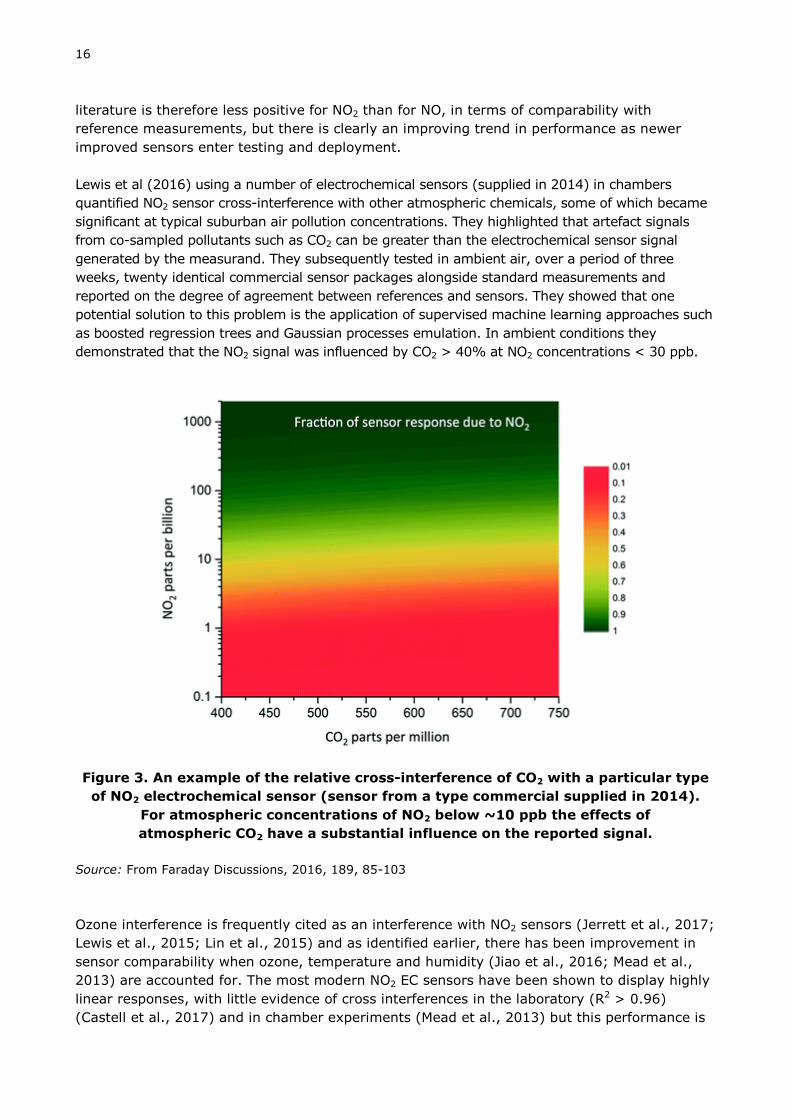
16

literature is therefore less positive for NO2 than for NO, in terms of comparability with reference measurements, but there is clearly an improving trend in performance as newer improved sensors enter testing and deployment. Lewis et al (2016) using a number of electrochemical sensors (supplied in 2014) in chambers quantified NO2 sensor cross-interference with other atmospheric chemicals, some of which became significant at typical suburban air pollution concentrations. They highlighted that artefact signals from co-sampled pollutants such as CO2 can be greater than the electrochemical sensor signal generated by the measurand. They subsequently tested in ambient air, over a period of three weeks, twenty identical commercial sensor packages alongside standard measurements and reported on the degree of agreement between references and sensors. They showed that one potential solution to this problem is the application of supervised machine learning approaches such as boosted regression trees and Gaussian processes emulation. In ambient conditions they demonstrated that the NO2 signal was influenced by CO2 > 40% at NO2 concentrations < 30 ppb.

Figure 3. An example of the relative cross-interference of CO2 with a particular type of NO2 electrochemical sensor (sensor from a type commercial supplied in 2014).

For atmospheric concentrations of NO2 below ~10 ppb the effects of atmospheric CO2 have a substantial influence on the reported signal.

Source: From Faraday Discussions, 2016, 189, 85-103

Ozone interference is frequently cited as an interference with NO2 sensors (Jerrett et al., 2017; Lewis et al., 2015; Lin et al., 2015) and as identified earlier, there has been improvement in sensor comparability when ozone, temperature and humidity (Jiao et al., 2016; Mead et al., 2013) are accounted for. The most modern NO2 EC sensors have been shown to display highly linear responses, with little evidence of cross interferences in the laboratory (R2 > 0.96) (Castell et al., 2017) and in chamber experiments (Mead et al., 2013) but this performance is

17

not fully replicated in the field, with larger discrepancies seen in ambient air (R2 between sensor and reference dropping to <0.65) (Castell et al., 2017).

For O3 measurements, electrochemical sensors are fast (about 60s), sensitive, and linear (Spinelle et al., 2015a). They generally suffer from NO2 quantitative interference from ageing and they can be affected by the daily variation of humidity and temperature or by rapid change of humidity (Spinelle et al., 2015a). MOS are very sensitive (lod < 2 ppb) and are likely not affected by cross sensitivities. They are slower than electrochemical sensors (> 5 min). Without correction/calibration, they are generally not linear and suffer from strong drift over time (Spinelle et al., 2016). As for electrochemical, temperature and humidity have an important effect on MOS sensors, the temperature effect being generally easier to correct (Spinelle et al., 2016). When using O3 electrochemical sensors in field, the comparison between sensor and co-located reference measurements generally gives good agreement with reference values (R² > 0.80) at sampling sites where O3 is higher than NO2, e. g. at rural sites (Spinelle et al., 2015b). Conversely at urban and traffic sites, electrochemical sensors have difficulties to measure low O3 together with high NO2 resulting for some sensors in low R². Among the short list of MOS field tests, a few have reported good agreement between sensors and reference measurements (R2 > 0.85) at urban background and rural sites provided that sensors were previously in-field calibrated (Lin et al., 2015; Williams et al., 2009). Caution is needed when generalizing between different brand models, different generations of the same sensor model and it depends whether or not post data treatment is applied.

Some electrochemical O3 sensors have been seen to under-predict absolute concentrations of O3 in controlled chamber experiments, but have presented strong correlation with reference measurements, meaning temporal patterns were accurately estimated (Castell et al., 2017). In-field ambient co-location with reference instruments has shown poorer correlation than when in the lab, but the sensors did still follow the reference instruments temporal pattern with high linearity in some cases (Jiao et al., 2016; Lewis et al., 2015). Other outdoor co-located O3 electrochemical sensors have had poorer reported correlations with the AQM reference (Jiao et al., 2016), indicating that performance can vary considerably from sensor to sensor.

Variability between identical sensor models is a further important characteristic to be defined before applications can be designed. In one study (Moltchanov et al., 2014), the averaged sensor signal from a large number of MOS O3 sensors displayed a good linear relationship between the reference instrument and the sensor reported concentration, but individual sensors deviated substantially from one another. A study further using MOS O3 sensors against a reference presented a high linearity between the two types of measurements but when comparing absolute concentrations, the sensors were typically under-predicting O3 at the lowest concentrations and over-predicting the episodic ozone peaks (Lin et al., 2015).

Tungsten oxide (WO3) based sensors were co-located with reference instruments outdoors at several locations (Auckland (NZ), Houston (Texas, USA) and Raleigh (North Carolina, USA)) to evaluate the abilities of LCSs to detect O3 in the real world, with similar results to that of several reference sites. The sensors showed a linear response to changing O3 concentrations monitored by the reference instruments although deviations between them were observed when the O3 concentration increased rapidly (Williams et al., 2013). In these studies corrections were successfully made for cross interferences, zero-air drifts and calibration for several short-term (max. four months) deployments for O3 sensors co-located with reference analysers (Williams et al., 2013).

18

The correlation between various different types of co-located CO sensors with reference monitors has been reported to be rather variable in ambient air, sometimes with rather poor non-linear responses when deployed outdoors (R2 0.18 – 0.48) (Jerrett et al., 2017), with absolute CO sensor concentrations sometimes not matching the reference and in other studies being offset to the reference instrument. (Castell et al., 2017; Jerrett et al., 2017). CO sensors have showed temporal drift and some divergence of signal (Jerrett et al., 2017), but this has been shown to be consistent enough to correct for, allowing improvement in CO sensor performance and measurement comparison with reference (Jiao et al., 2016). Co-located low-cost CO MOS sensors in a further study did not follow the reference measurements at all and were non-linear (R2 = -0.4- -0.14). In the case of CO, the exact type of sensor being used is therefore critically important, since a wide range of data qualities can be experienced dependent on this.

Sulphur dioxide is infrequently measured with LCSs due to issues with limit-of-detection in many ambient environments. In locations where there have been large-scale policy-driven mitigation efforts (United States, much of Europe) and SO2 levels have been reduced below regulated limits, LCS measurements for SO2 are often ineffective. Studies which have been performed in such areas show little correlation to reference data (usually with SO2 < 5 ppb) (Borrego et al., 2016). However, recent literature (Hagan et al., 2018) has shown promise for using LCSs for SO2 in environments where SO2 levels are sufficiently high which could be relevant for many countries in developing economies which still rely on high sulphur-content fuels, areas with high presence of sulphur-emitting industry, and areas near large point sources of SO2 such as volcanoes. In these instances, LCSs for SO2 have been shown to be effective when SO2 concentrations exceed 10 ppb.

Total volatile organic compounds are less widely monitored because reference instrumentation is not as widely available and the alternative sensors themselves are not compound selective. Sensors provide a bulk VOC measurement whereas reference instruments give a speciated measurement (e.g. concentrations of specific organic compounds). While sensors (either MOS, or photoionization detectors) can notionally report a total VOC concentration, they exhibit varying sensitivities towards different groups of VOC and this is challenging to correct for (Smith et al., 2017). MOS sensors have been co-located with a Selected Ion Flow Tube (SIFT) Mass Spectrometer (MS) indoors (a technical measurement of specific VOCs). At concentrations of 300 ppb or lower the sensors closely matched the response of the reference, but there was a high degree of non-linearity at higher concentrations. The LCSs displayed slower response times to peaks in VOC concentrations and a non-additive response when mixtures of VOC were injected, rather than individual compounds (Caron et al., 2016).

3.2 Low-cost sensors for Particulate Matter (PM) Particle measurements, when categorized across different sizes are far more complex than gas measurements and depend on a variety of factors which differ for different measurement methodologies and for different particle types (chemical composition, density, relative humidity, refractive index, shape and size distribution). Particles can also be highly reactive, and reported mass concentrations are subject to sampling biases if during the process of being sampled, the particles are transferred across strong temperature/humidity gradients. Low-cost PM measurement techniques most commonly rely on optical (light-scattering-based) measurements of PM, which typically use a low-power light source – either an LED or laser – where particles that are collected scatter light measured by a photo detection device.

19

Concentration is proportional to the scattered light intensity and a particle density and size distribution is usually assumed. There are two broad measurement techniques employed by LCS applications including nephelometry which measures particle light scattering of an ensemble of aerosols, and optical particle counting which measures particle size and number of individual particles. Neither technique directly measures particle mass but are usually statistically related to particle mass measured by a reference measurement.

The size detection limit of most low-cost light scattering devices for particle number (PN) concentration measurement can only observe particles in the ~400 nm – 10,000 nm size range, and are generally insensitive to particles outside of this range (Wang et al., 2010). This is particularly relevant for the determination of total PN concentrations. This can be relevant near roadways which are usually dominated by particles less than 400 nm in diameter. There are no low-cost sensors available that detect ultrafine particles, which are generally defined as particles less than 100nm in diameter; in lower cost systems light scattering is limited to the detection of particles with a diameter >300nm.

Limits of detection in the 1-10 µg m-3 range have been reported for low-cost optical particle counters (Holstius et al., 2014; Jovašević-Stojanović et al., 2015; Kumar et al., 2015), though this is usually estimated under more optimal laboratory conditions. Such sensors have been shown to have non-linear calibration with two or more response functions. They also have upper detection limits, typically in the range of 500-1000 µg m-3, making them unsuitable for extremely polluted locations.

The most significant interfering variable seen with low-cost PM sensors relates to water, and they appear susceptible to variable and unpredictable performance under conditions of high relative humidity. Recent studies suggest a degradation in performance when relative humidity exceeds 80-85% (Crilley et al., 2018). There are also likely to be chemical composition effects associated with particle hygroscopicity that interact with the humidity effect. That is, there may be some mixtures of aerosols that are more susceptible to relative humidity influences than others. At present, this is an emerging field of study, but it is clearly an important factor to resolve for future possible applications of PM low-cost sensors, since it makes calibration of such devices composition-dependant.

To date, there are typically few, if any, built-in QA/QC tools available in most low-cost PM sensors to correct or adjust data and like reference monitors calibration is based on more infrequent testing against known aerosol sources. The application of external standards is required to assess instrument performance in a field location to account for sensitivity or response drift, or to validate data during data collection. In this regard low-cost sensors and reference devices can potentially share the same kinds of quality assurance framework and standards, although at present the long-term (> 1 year) stability of low-cost PM sensors remains uncertain.

There are a few low-cost devices available that can provide a measure of particle size distribution, but such LCS options generally offer only a relatively coarse size resolution. Typically data from such devices may place particles into anywhere between 6 and 32 size bins. There are currently no LCS devices capable of measuring the size distribution of ultrafine particles, and these types of particles can only be assessed at present with reference instrumentation and techniques.

20

Though they are often based on similar analytical principles, a number of key differences exist between low-cost and reference equivalent optical PM instruments: (1) reference equivalent optical instruments maintain a constant relative humidity within the sampling inlet of the system (they dry particles) whereas low-cost PM sensors operate at ambient relative humidity which leads to different results depending on particle hygroscopicity; (2) reference equivalent instruments are comprised of precision optics (for focusing laser light and collecting scattered light), superior particle flow control, and highly sensitive optical detectors, the combination of which allows for much lower background noise and improved detection of smaller particles. Literature does however support that: (1) low-cost approaches can be useful for qualitative assessment of particle concentrations in a moderately polluted environment, and that; (2) deployment of many sensors on a community or neighbourhood-scale can provide sufficient data granularity to provide insight into spatial and/or temporal patterns and source apportionment. This may be useful for refinement of modelling approaches, assessing human exposures, or producing datasets for long-term trend analysis, once known LCS limitations are resolved.

3.3 Low-cost sensors - greenhouse gases Greenhouse gas sensors often use miniaturised versions of optical absorption methods that can also be found in reference instruments. The evaluation of their performance is therefore more straightforward in that similar approaches to testing can be applied to sensors. This section gives an overview of most common low-cost measurement methods for greenhouse gases and provides a brief overview of laboratory experiments and field projects that have compared sensor scale devices for greenhouse gases (GHGs) against reference instruments.

Comparatively few studies using sensors for atmospheric measurements of GHGs are available in the literature. Most of them have utilized sensors for CO2 and only very limited number of publications were found examining sensors for CH4 (Collier-Oxandale et al., 2018; Eugster and Kling, 2012; Suto and Inoue, 2010). For CO2, LCSs are based on non-dispersive infrared absorption (NDIR). NDIR is a technique in which infrared light is absorbed by sampled CO2, where the amount of light absorbed is proportional to concentration. The CH4 sensor in (Collier-Oxandale et al., 2018; Eugster and Kling, 2012; Suto and Inoue, 2010) was based on a metal oxide semi-conductor as the gas sensing material.

Shusterman et al. (2016) presented the use of a NDIR absorption sensor in each node in a network (BEACO2N). An advantage of such techniques is that performance can to a degree be evaluated from first principles knowledge of instrument features such as path length and absorption properties of the specific gas of interest. Some low-cost greenhouse gas sensors have been shown to possess adequate sensitivity to resolve diurnal as well as seasonal phenomena relevant to urban environments (Rigby et al., 2008) and in hardware terms, have costs that are one to two orders of magnitude lower than commercial cavity ring-down instruments commonly used in global carbon tracking networks.

Most of the published studies using LCSs for CO2 have focused on the characterization of the sensor performance from comparison against reference instruments under field conditions. Spinelle et al., (2017b) evaluated the performance of two types of low-cost NDIR sensors from field tests. This group used different statistical and machine learning approaches to evaluate their data and assess (and correct for) interfering factors such as ambient temperature and relative humidity. The best results were achieved using machine learning techniques such as

21

Artificial Neural Networks (ANN), where sensor uncertainty was 5% in the range from 370 to 490 ppm CO2 (typical ambient concentrations) but increased up to 30% when a less sophisticated linear regression model was applied. It should also be noted that these results were only obtained with simultaneous availability of a reference instrument during the first 10% of the comparison period. This suggests that in some cases, uncertainty will be higher when using less sophisticated machine learning techniques to calibrate instruments.

The performance of different data models for the correction of a NDIR sensor signal operating under field conditions was explored in the study by (Zimmerman et al., 2018). It was again found that a machine learning technique (Random Forest models) outperformed multiple linear regression models. The absolute mean error of the CO2 sensor measurements was reported to be 10 ppm during a 16-week testing period. It should, however, be noted that the sensor performance was evaluated using training and test data measured at the same field location and that the applied calibration model included the signal of a separate CO sensor as an interfering factor. The transferability of the determined correction model to locations with different relationships between CO2 and CO might therefore be limited. This is a generic issue for LCSs in that sophisticated data models can often help improve LCS data such that there is excellent local agreement against reference monitors, but the extent to which the model is applicable to other locations is less clear.

A study by Kunz et al., (2017) showed that it was possible to use small and inexpensive sensors for atmospheric measurement of CO2 with an accuracy that was sufficient for targeted applications. It seems, however, inevitable that the sensor units must be individually tested and corrected for their response to changing temperature, pressure and relative humidity (when the air sample is not dried). A reasonable way to do this may be test measurements in environmental chambers followed by verification of the applicability of the determined data correction parameters through comparison of the resulting sensor signal with reference instruments during field tests. When sensors are then deployed away from reference instruments, strategies for continuous quality assurance and quality control of the sensors must be implemented; an example methodology is outlined and applied in Kunz et al., (2017). This is of course not specific for sensors for GHGs but applies to all sensors for atmospheric gases and particles.

In publications that have used sensors for atmospheric CH4 (Eugster and Kling, 2012; Suto and Inoue, 2010), the sensor response was found to be sensitive to ambient temperature and relative humidity. Based on measurements under field conditions in Alaska (Eugster and Kling, 2012), it was concluded that the relative concentration derived from the sensors was sufficient for preliminary observations needed to locate potential methane (CH4) hotspots. However, correction of the temperature and humidity cross-sensitivity was required, and the performance of the sensors was not sufficient for long-term studies where accurate methane measurements were needed. Removal of water vapour to less than 10 ppm as well as catalytic conversion of other flammable gases was needed for the sensor system used in Suto and Inoue (2010), in order to allow for monitoring of atmospheric methane.

Collier-Oxandale et al. (2018) investigated low-cost methane sensing approaches at two different deployments, at sites near active oil and gas operations and in an urban neighbourhood subject to complex mixture of air pollution sources including oil operations. Field normalizations were used to generate calibration models for the sensors, which included co-locating the LCS systems with reference instruments for a given period. They concluded that those particular types of sensors would likely never replace traditional air quality

22

monitoring methods, but they could provide useful supplementary information on local pollution sources.

3.4 Mobile sensors A large majority of existing low-cost air quality sensor systems target a static deployment scenario. However, the idea of using mobile sensing in the context of air quality monitoring has been gaining momentum over the last decade, with sensing systems using mobility vectors including private citizens (Bales et al., 2012; Mead et al., 2013), bicycles (Elen et al., 2013), and public transportation vehicles (Aberer et al., 2010; Castell et al., 2014). As is the case with other sensing applications, one of the main advantages of mobile sensors lies in the potential of extending spatial coverage for a given number of sensor units. Moreover, for the case of exposure evaluation in outdoor environments, considering the mobility of the sensor system is indispensable. The implementation of sensors on mobile platforms can however lead to a significant degradation of the sensor’s performance, depending on the underlying sensor technology, but also on its integration within a sensing system. We summarize here some of the documented adverse effects that can arise when using low-cost sensors for mobile measurements. Electrochemical and metal-oxide sensors have response times that range from tens of seconds to multiple minutes. While for static deployments, this issue can be largely neglected, for mobile sensing systems it can induce significant distortion of the measured signal with respect to the underlying concentration levels. This effect can be viewed as analogous with motion-blurring in photography, which happens when the exposure time of a camera system is long relative to its movement speed. The severity of the distortion will vary depending on the speed of the mobile platform (Arfire et al., 2016) and will need to be evaluated. The sensitivity of electrochemical sensors to variations in relative humidity can be a challenge for mobile measurements that include various different types of environments (e.g. both indoor and outdoor). The abrupt changes in relative humidity that can occur between indoor and outdoor environments, for instance, can lead to aberrant measurements. Finally, for all low-cost sensor systems used for mobile applications (i.e. including PM sensors), special care needs to be given to the design of the air sampling system to reduce performance degradation due to poorly controlled flow conditions.

4. EVALUATION ACTIVITIES FOR LCSs

Over the past decade there have been worldwide efforts to evaluate the usefulness and possible applications of LCS technology. Performance evaluation projects have focused on determining the quality of the data produced by sensor systems by comparing their response to reference instruments in the laboratory and in the field. Complementary to this, demonstration projects have explored how the use of these sensor systems may give new insight into atmospheric processes. There are many interested users; performance and demonstration projects have engaged governmental

There have been worldwide efforts to evaluate the usefulness and possible applications of low-cost sensor technology.

23

organizations, research groups, city departments, and community and citizen science groups all seeking to understand how LCSs may be used. The following two sections provide examples illustrating some recent performance evaluation and demonstration efforts, and what lessons might be drawn from these.

4.1 Performance evaluation programmes

Performance evaluation programmes have been undertaken by many different organizations, all seeking to evaluate in quantitative terms how LCSs compare against reference measurements in laboratory and ambient sampling conditions. Laboratory evaluations allow researchers to control conditions and examine the response of sensors to different temperatures, relative humidity, a range of gas or particle concentrations, and other potential interfering factors. Evaluation in outdoor conditions provides a more “real-world” test of the sensor systems but may be limited to the range of atmospheric conditions experienced at a particular location and some interfering variables may not be visible or measured during the test phase.

Figure 4. Scatter plots showing a range of LCS performances during a real-world test: (a) good agreement between a PM sensor system and reference instrument;

(b) reasonable agreement for O3, and; (c) poor agreement for NO2. Scatter plots show results from field evaluations of an individual sensor system performed by the Air Quality

Sensor Evaluation Programme. (http://www.aqmd.gov/aq-spec).

Several independent and foundational evaluation efforts are occurring in Europe and the U.S. These efforts are characterizing the performance of specific air monitoring sensors as well as generating resources for educating researchers, community groups, and the public about the advantages and real-world limitations of such sensor systems. Such studies also highlight the need for simple common data quality indicators. In all cases, results from sensor analyses are manufacturer and model specific, and one should not assume all sensor models for a particular compound will perform as indicated here. Typically such evaluations have focused on comparing a small number of examples of sensor systems from individual manufacturers but there is a growing awareness of the need to test the variability between batches of identical sensors. The Joint Research Centre (JRC) has been evaluating air sensors since the late 2000s. They have a laboratory for evaluating gas sensors and have conducted many laboratory and field evaluations of sensor systems. Initial efforts focused on evaluating O3 and NO2 sensors (Aleixandre and Gerboles, 2012b; Penza et al., 2014). For O3, an evaluation of metal oxide sensors in laboratory conditions (Spinelle et al., 2016) showed slow response times,

24

non-linear relationships with reference data, limits of detection of several ppbs, but little to no interference with other gases (NO2, NO, CO, CO2 and NH3). Longer-term (more than six months) evaluations however have showed that changes of temperature and humidity could generate measurement uncertainties over 100%. For ozone and nitrogen dioxide electrochemical sensors, a laboratory evaluation (Spinelle et al., 2015b) showed a good linear response, appropriate ambient limit of detection and a repeatability better than 10 ppb. When testing the interference effects of O3, NO2, NO, CO, CO2 and NH3, it was found that O3 sensors were only affected by NO2 while NO2 sensors were also affected by O3 with interference in the order of 100%. The longer-term drift (more than 6 months) of electrochemical sensors was less than that for MOS equivalent devices. More recently JRC evaluated performance of benzene and VOC sensors (Spinelle et al., 2017a). The conclusion was that current sensor technology was not able to accurately and selectively measure benzene at ppb ambient levels (there is a limit value of 1.5 ppb in the European Air Quality Directive). A wider conclusion was that calibration of these sensors is critical and JRC explored several calibration methods including linear regression, multiple linear regression, and artificial neural network (Spinelle et al., 2015b, 2017b). The artificial neural network was preferred for NO2/O3 and led to uncertainties of less than 20%. JRC continues to conduct a wide range of other research on sensor systems including developing a protocol for evaluating sensors (Spinelle et al., 2013) and development of open source AirSensEUR sensor platform (Kotsev et al., 2016). EuNetAir Air Quality Joint Intercomparison Exercise organized in Portugal focused on the evaluation and assessment of environmental gas, PM and meteorological microsensors, versus standard air quality reference methods through an experimental urban air quality monitoring campaign. A mobile laboratory was placed at an urban traffic location in the city centre of Aveiro to conduct continuous measurements with standard reference analysers for CO, NOx, O3, SO2, PM10, PM2.5, temperature, humidity, wind speed and direction, solar radiation and precipitation. Approximately 200 sensors were co-located at this platform. Overall, significant differences were observed across the different sensors being tested. Some sensors were in good agreement with the reference, but with others substantially disagreeing. As an example, the range of correlations between different sensor types and reference instrument O3 were in the range R2: 0.12 - 0.77, for CO (R2: 0.53 - 0.87), and NO2 (R

2: 0.02 - 0.89). For PM (R2: 0.07 - 0.36) and SO2 (R

2: 0.09 - 0.20) the results showed a poor performance with low correlation coefficients between the reference and sensor measurements (Borrego et al., 2016). Again a simple conclusion was that even sensors measuring the same parameter can show very different levels of performance when compared to a reference, depending on the device and manufacturer. U.S. Environmental Protection Agency (USEPA) began evaluating air quality sensors in 2013. Initially these efforts comprised laboratory tests of O3 and NO2 sensors and these showed: (1) very fast response times with minimal rise and lag times which suggests potential use for continuous or near-continuous environmental monitoring; (2) a high degree of linearity over their full response range at concentrations; (3) detection limits higher than reference instrumentation; (4) cross-sensitivity interference from other gases (e.g. NO2, O3, SO2), and; (5) high relativity humidity and temperature resulted in some undesirable response characteristics (Williams et al., 2014). Later field studies of sensors measuring NOx, O3, CO, SO2, and particles revealed more variable performance when compared to reference monitors (Jiao et al., 2016). USEPA continues to conduct a wide range of sensor development,

25

evaluation, and demonstration projects with results published on their Air Sensor Toolkit website (https://www.epa.gov/air-sensor-toolbox). The South Coast Air Quality Management District (Los Angeles, USA) started the Air Quality sensor performance evaluation center (AQ-SPEC) in 2014. The center’s goal is to provide guidance on the performance and application of sensors, promote use of sensor technology and minimize confusion with users purchasing and using new LCSs. The pollutants covered included the key EPA criteria pollutants and some air toxics. The AQ-SPEC programme has provided a method to evaluate the performance of a range of different devices and sensor data. Work involved both laboratory and field testing (data from this programme is shown in Figure 4). A number of reports (~30) from field tests of different sensor types appear on the AQ-SPEC website (http://www.aqmd.gov/aq-spec/evaluations/field). Field evaluations have generally indicated performance of CO, NO, O3 sensors as being the most encouraging, a number of oxidant sensor (e.g. O3/NO2) measurements were problematic (due to interferences), and SO2, H2S & VOC measurements were not in good agreement with reference monitors at this location. PM2.5 sensors had in general a high correlation with EPA-approved instruments, but PM10 was more divergent and it was noted that continuous sensor calibration was needed; very small particles (0.5 µm) were not detected at all and conversion between mass and particle numbers was not straightforward.

4.2 Low-cost sensor demonstration projects The earlier section referred to some examples of recent studies to quantify the performance of sensors by evaluating them in the laboratory or under field conditions. Rapid product development, low-cost, and relative ease-of-use is also resulting in deployment of distributed networks to demonstrate the value and usefulness of sensor systems in the field. Such experiments do not aim to necessarily provide precise side-by-side comparison data with reference monitors but instead show how a sensor-based approach may give additional insight into atmospheric composition. Demonstration projects have engaged both traditional users and new communities not previously part of traditional air monitoring networks. Newer users are often interested in using sensor networks to understand local air quality conditions, to identify local sources, implement educational/outreach programmes, and identify appropriate mitigation strategies where applicable.

Citizen science initiatives have been a particularly significant fraction of demonstration projects; some projects have been in partnership with traditional research institutions (universities, governmental agencies, or industry) while others have been managed entirely by private sector groups or individuals interested in air quality. LCSs represent a clear opportunity to support citizen science initiatives, and make new measurements in low and middle-income countries which are often understudied by the public health and atmospheric science research communities.

Though the intent of most citizen-science projects is to gain insight into questions of local air quality, it is often not possible for external audiences to fully discern the quality of the data collected. To date, the evidence collected from recent studies is most useful in understanding the logistical features of citizen science itself, including salient issues of pragmatism - is possible to recruit willing participants,

LCS represent a clear opportunity to support citizen science initiatives, and make new measurements in low and middle income countries which are often understudied by the public health and atmospheric science research communities.

26

and assess the types of questions that communities wish to address? Some of these projects include United Nations Development Programme, Ministry of Data Balkans Green Machine Team, the CityOS project in Sarajevo, Bosnia & Herzegovina, and the Air pollution Interdisciplinary Research (AIR) Network in Kenya.

There are however a number of demonstration projects using sensors that include experienced users and research organizations where insight into both the technical process of sensor use and more quantitative outcomes can be obtained. An example is the BEACO2N project in Northern California (Kim et al., 2017; Shusterman et al., 2016; Turner et al., 2016) which is a multi-pollutant sensor project using a distributed network of approximately 50 sensor “nodes”, each measuring CO2, CO, NO, NO2, O3 and particle matter at 10 second time resolution at approximately 2km spacing in locations surrounding the San Francisco Bay Area.

The preliminary analysis of the first three years of CO2 observations provided evidence of the expected diurnal and seasonal cycles as well as an encouraging sensitivity to short-term changes associated with local emission events. Further work is proposed to fully assess the efficacy of inverse methods based on the BEACO2N approach, however it constitutes a promising infrastructure upon which further advances in high-density atmospheric monitoring can be built. The network has also provided insight into calibration models for CO, NO, NO2, and O3 that make use of multiple co-located sensors, a priori knowledge about the chemistry of NO, NO2, and O3, as well as an estimate of mean emission factors for CO and the global background of CO. The Zurich O3 & NO2 network (Mueller et al., 2017) was a blended network of LCSs co-located near to a regulatory network of reference air pollution monitors in Zurich. O3 and NO2 low-cost gas sensors were shown to provide concentration measurements with an accuracy of a few ppb in the first 1-3 months of operation. Comparisons with diffusion tube measurements and measurements from AQM sites revealed that this accuracy could not be maintained during the entire 1-year network deployment due to the changing response behaviour of the sensors. Several issues were encountered that were related to the type of sensors used that caused temporary (∼ hours) or persistent decrease of sensor accuracy. Hence, the application of performance monitoring strategies has been advised as a prerequisite when operating LCSs with such properties in order to be able to assess the quality of the data.

All the sensors in this network required individual cross-referencing to reference monitors. Sensor co-location next to reference sites was found to time consuming and required considerable traditional infrastructure. Moreover, the quality of the compiled calibration data set for the model parameter estimation depended on the prevalent ambient conditions (i.e. encountered pollutant concentrations, meteorology). The NO2 sensors were heavily impacted by changes in relative humidity. This effect could be reduced to a certain degree by the application of a correction function but still limited the achievable accuracy of the sensors. This issue points to the necessity of an improved mathematical description of the sensor based on its working principle in order to describe sensor behaviour in more detail. More sophisticated sensor models may facilitate calibration as its parameters could be constrained with less effort than is required when applying regression models.

NO2 and O3 concentration predictions could be derived at the level of a few ppb at specific time periods for many locations in Zurich using the data from the AQM network which covered a wide range of different pollutant situations. This feature can be a substantial factor for an

27

effective monitoring of the sensor performance in LCS networks. Moreover, such data can be used for the remote correction of sensors. In this study this procedure was shown to improve the results of NO2 sensors.

The Hong Kong Green Marathon sensor network (Sun et al., 2016) was an ad hoc sensor-based air quality monitoring network with 6 sets of sensor systems deployed along the marathon route, including electrochemical based NO2, CO, O3 and photometer based PM2.5 measurements. Real-time monitored air pollution concentration data were transmitted back to the server centre with Air Quality Health Index (AQHI) calculated on an hourly basis. Intensive quality assurance and quality control measures were conducted for sensor calibration and data quality control. High linearity of sensor response to the pollutants in the laboratory was observed. Due to the short deployment period, a relatively narrow variation of temperature and relative humidity conditions during the field test made it favourable to use simplified sensor equations with good performance when comparing to side by side reference data in AQM stations. High correlation coefficients (>0.96) were all observed for NO2, CO and PM2.5 between the sensor systems and the reference instruments. The air sensor network data from the roadside of a busy main road during and after the marathon event showed the effectiveness of temporary traffic control on creating a significant reduction of concentrations of traffic-related air pollutants, such as NO2 and CO. According to the tunnel sensor node, mechanical ventilation demonstrated a substantial impact on improving the air quality.

The Location Aware Sensing System (LASS) project in Taiwan currently has more than 5000 devices deployed in 36 countries. This network includes low-cost PM2.5 sensing devices (USD 100-500) from commercial products, internet maker groups, and scientist research groups, with 2 or 3 different PM2.5 sensor components (Chen et al., 2017). This network is evolving rapidly as a collaboration among research groups, governmental agencies, NGOs, and commercial companies, including efforts by citizen scientist ”Makers”. The data is displayed in a near real-time with several options of visualization (https://airmap.g0v.asper.tw/) and the data portal is maintained by Academia Sinica (https://pm25.lass-net.org/en/). Roughly 100 of these sensor devices have been calibrated in the laboratory and the field against reference instruments, with reported correlation coefficients exceeding 0.80. Different calibration curves are needed for different concentration ranges such as <30, 30-150, and >150 ug/m3, and sensor precision is reported to within 20% variability. An anomaly detection framework for large-scale PM2.5 sensing systems is used to detect sensor malfunction and spatio-temporal anomalies has been proposed using data analytics (Chen et al., 2018). The following scientific challenges and opportunities arise: (1) this network is comprised of PM2.5 sensor components with different stability, variability, and sensing frequency; (2) the vast number of the devices require big data analytics to make sense of the measurements; (3) the network has potential applications in different research fields with participatory approaches; and (4) the network can potentially be used in validation and development of fine-resolution air pollution transport and dispersion models.

An Italian national project RES-NOVAE - Networks, Buildings, Streets: New Challenging Targets for Environment and Energy deployed one mobile and 10 stationary nodes which were installed in specific sites (buildings, offices, schools, streets, port, airport) to enhance citizen’s environmental awareness. Continuous measurements were performed by low-cost electrochemical gas sensors (CO, NO2, O3, SO2), an optical particle counter (PM1.0, PM2.5, PM10), an NDIR infrared sensor (CO2), and a photoionization detection (total VOCs), including

28

microsensors for temperature and relative humidity. As an example, the Mean Absolute Error (MAE) of PM10 for three locations was 5.6 µg/m3, while the accuracy was around 25% (Penza et al., 2017). In summary, larger multi-node sensor networks based on LCSs have already been deployed as test projects in a number of locations around the world, and the above examples or only illustrative examples, many more exist. The most important area of uncertainty from the current round of demonstration studies is how to most effectively utilize these new measurements given that there are known issues regarding data quality and the stability of responses over time. There is a particular lack of data at present from demonstration projects running long-term – that is over the course of a year or longer. Care should be taken to understand the exact intentions of each demonstration study, for example whether the projects were designed to test the ability of a network to quantify air quality or greenhouse gases, or whether the network was used to test the technical feasibility of deployment, citizen engagement or wider issues associated with deploying a sensor network.

5. CALIBRATION AND QUALITY ASSURANCE/QUALITY CONTROL OF LCSs

There is a wide range of users of LCS devices, and the user (and application) will dictate the necessary level of data quality. For example, devices positioned as hobby/consumer products will have lower expectations than those used for operational air pollution management or controls. LCSs challenge the status quo and therefore will need adoption of new and different approaches for QA/QC to those currently used for the measurement of air pollution and greenhouse gases. Any methods applied to LCSs must however be capable of direct comparisons to QA/QC approaches used for reference measurements.

While various stakeholders will have different requirements for accuracy and traceability, it is imperative that there is a transparent characterization of how a given sensor behaves – after all, “data of poor or unknown quality is less useful than no data since it can lead to wrong decisions” (Snyder et al., 2013). To address this issue, there is a critical need to establish a cohesive approach for the evaluation and performance assessment of LCSs prior to their large-scale adoption in atmospheric science (Lewis and Edwards, 2016). Activities such as CEN TC 264 Working Group 42 is one example of an international coordinated effort to address these issues for reactive air pollutants.

That being said, air pollution sensors should be treated as any other analytical instrument; they will likely require regular calibration and will show long-term changes in drift and sensitivity. For the purpose of this document, we define a calibration of a LCS as the establishment of a relationship between the output of a LCS and a measurement standard, where a measurement standard in this context can be either a calibrated reference instrument or a gas/particle reference material. It should be appreciated that this definition on calibration falls within the definition of the term as recognised by WMO but such an approach is not necessarily viewed as being calibration by some National Metrology Laboratories.

“Data of poor or unknown quality is less useful than no data since it can lead to wrong decisions” (Snyder et al., 2013).

29

5.1 Calibration and Quality Assurance The calibration of LCSs involves determining a model that can be used to convert between the measured parameter (e.g. light absorption, voltage, or conductivity) and desired output variable (e.g. pollutant/species concentration). Typically, this is fairly transparent, with factory calibration settings published in component data sheets. At present, it is likely many users continue to rely on these factory calibration settings as the main method of calibration. However, there is limited evidence to suggest, at least for the current generation of LCSs, this is sufficient to provide long-term accurate data across the possible environments in which the sensor may be used. To determine whether or not a factory calibration is sufficient, a validation (quality assurance) of the data should be performed in an environment similar to the one in which the LCS will be used.

Figure 5. A schematic of typical levels of validation of sensors and instruments

Currently, there are two main approaches to calibrating LCSs: laboratory calibration against reference materials and field co-location with reference monitors which have themselves been calibrated against reference materials; both methods have benefits and drawbacks. Laboratory calibration typically involves the same approaches used to calibrate reference and research-grade analytical chemistry instruments: subjecting the sensor to a series of known concentrations of pollutant/species using known measurement standards in a controlled environment. This approach has been explored extensively in the literature (Castell et al., 2017; Mead et al., 2013; Piedrahita et al., 2014); unfortunately, the conditions under which sensors are calibrated in the laboratory do not often overlap with the full range of conditions encountered in an ambient environment. These differences include the presence of cross-sensitive gaseous species (Lewis et al., 2015), changes in relative humidity and temperature, and ever-evolving aerosol physical and optical properties, all of which are known sources of error for LCS measurements. Laboratory experiments are also limited to those with the resources and/or opportunity to access the necessary equipment, which may not be all future user groups of LCSs. However, laboratory experiments can be very useful for determining how LCSs behave under very specific, controlled conditions which contribute to our fundamental understanding of how they work. If using a laboratory test as a primary calibration approach,

30

it is important to mimic the deployment environment of the sensors as closely as possible (e.g. using an environmental chamber to scan the typical range of temperature, humidity, pressure, etc.).

To overcome some of the limitations encountered in the laboratory, many have found ambient co-location against reference monitors to be an effective method whereby calibration parameters can be applied to a LCS. Here, the sensor (or sensors) is placed in the field near a reference instrument for a period of time to provide a direct comparison of the LCSs output to that of a calibrated reference instrument. It can be difficult however to experience the entire dynamic range of target species, cross sensitive species/pollutants and environmental parameters in a short period of time and this can make comprehensive calibrations rather time intensive. Access to locations and calibrated reference equipment can also be an issue, and a LCS user must ensure that an accurate clock record (e.g. local time or universal time) is maintained. The seasonal change of the field environmental conditions should be considered (in addition to the LCS drift) to determine the frequency of the field co-location calibration. When planning and performing a calibration of a LCS, important factors to consider are temperature, relative humidity, and cross-sensitive gas species (details can be found often in data sheets and in literature) for gas-phase sensors, and relative humidity, composition, density, size distribution, and optical properties for particle sensors. As described in earlier sections, PM measurements using LCSs do not map easily only reference data or to the more commonly used PM mass metrics used in air quality standards. For both approaches mentioned above, an active area of research is determining the optimal algorithm used to convert raw sensor data (often current or voltage for gas-sensors, histogram or raw counts for particle sensors) into a usable format (concentration, mixing ratio, aerosol loading). Many have used variations of a parametric regression with some success (Jiao et al., 2016; Lewis et al., 2015; Masson et al., 2015; Mueller et al., 2017; Popoola et al., 2016; Sadighi et al., 2017; Smith et al., 2017) though many nonparametric/non-linear/machine-learning approaches have appeared recently in the literature (Cross et al., 2017; Hagan et al., 2018; Spinelle et al., 2015b; Zimmerman et al., 2018) as they can account for less obvious environmental effects and interference with cross-sensitive species. Regardless of the calibration/data correction methods having a framework to compare different sensors and algorithms is useful, if only to evaluate in a standardized way how each improves or degrades the quality of data compared to a reference. Many studies currently use a combination of the correlation coefficient (R2), root mean squared error (RMSE), and mean absolute error (MAE) to describe their model performance. While these are valuable, it is equally important to record, report, and understand the conditions under which a calibration was performed. Both particle and gas-phase sensors are limited in their ability to overcome certain measurement artefacts due to their underlying principle of operation. In addition, extrapolation of results from a short calibration period to a significantly longer time periods can pose a challenge. An active area of research is focused on determining drift over time, with reported drift timescales varying from days (Smith et al., 2017) to several months (Hagan et al., 2018; Mead et al., 2013; Popoola et al., 2016) for gas-phase LCSs. For low-cost particle sensors, it is crucial to be able to report on similarities and differences among the patterns of

Important factors to consider are temperature, relative humidity, and cross-sensitive pollutants for gas-phase sensors, and relative humidity, composition, density size distribution, and optical properties for particle sensors.

31

behaviour of LCSs and reference measurements, and to also record and report the type of aerosol and any available meta information (aerosol physical and optical properties, size distribution, meteorological conditions) as there are large, known errors associated with using optical measurement techniques to measure aerosols of rapidly changing composition and size distribution. Discerning these artefacts becomes especially difficult when using a reference instrument that uses the same underlying operating principle (e.g. optical light scattering) and therefore suffers from similar sources of bias and measurement uncertainty. Many manufacturers routinely provide factory setting sensor calibration data, which is often developed under proprietary laboratory conditions. Sensor responses may well be altered when used under different measurement conditions (i.e. calibration coefficients under ambient measurements are often different from the ones under laboratory conditions), and therefore, reliance on manufacturer calibrations alone, without reference comparison, is insufficient for quantitative data applications. 5.2 Quality control of sensors and sensor networks Quality control is the act of monitoring the long-term performance of a LCS during deployment in a sensor network to ensure it remains in calibration, and can help notify the appropriate party when a LCS needs to be corrected or removed and undergo re-calibration, likely when the bias exceeds the measurement uncertainty. Like their reference instrument counterparts, LCSs have a limited service lifetime, but this has yet to be determined for many LCSs, and can depend greatly on the environment in which a LCS is deployed (e.g. high pollution environments can cause PM sensors to foul, low humidity environments can cause sensitivity decay in electrochemical gas sensors). Quality control is ultimately also the method for determining end-of-life for a sensor. A user should apply quality control statistics to define the end-of-life for LCSs if using them over a sufficiently long period of time. There are several LCS parameters that should be monitored over time including baseline drift (change in intercept) and changes in sensitivity (e.g. changes in slope). If these values are known or can be calculated, data can be corrected over time with data post-processing (data correction). Several approaches to quality control have been proposed in literature. One approach is to periodically compare the values obtained with a LCS to a nearby (but not co-located) reference monitor (Mueller et al., 2017). In some locations, especially those throughout Europe and the United States, reference data is made available by regulatory agencies and can be accessed either through their websites or via public groups such as OpenAQ (https://www.openaq.org). However, it is important to be aware of possible limitations with this approach, since the concentrations of some reactive gaseous species (e.g. NO, NO2, CO, O3) may vary significantly, even over modest spatial lengths of a few meters. A second approach that has recently appeared in the literature, is to use knowledge of regional atmospheric chemistry in combination with a small number of anchor points (reference stations) to perform remote calibrations (Kim et al., 2017). Similarly, statistics-driven quality control checks based on transport phenomena could provide information on relative differences amongst sensors within a localized network.

There are several LCS parameters that should be monitored over time including baseline drift (change in intercept) and changes in sensitivity (e.g. changes in slope).

32

Figure 6. Span of current capabilities and applications across different types of air pollution measurement networks

While these approaches are still under active development, they do appear to be promising methods that could increase consistency of data, save time and effort and support quality checks on large numbers of sensors, especially as sensor networks move from tens of sensors to thousands of sensors. In this work we can refer only to studies where approaches are described in the open literature. There are some proprietary methods for large-scale LCS data QA/QC for networks being offered by manufacturers, but the technical basis for these is often not clear, and cited as commercially confidential. The open publication of principles behind large-scale QA/QC approaches is strongly encouraged.

Moving forward, as public interest in the utility of sensor networks continues to grow, it will be important to develop and refine new calibration and quality control approaches that allow users to better understand the quantitative capabilities of their sensors. Refining both the techniques used as well as the ways in which researchers, industry, and stakeholders validate the performance of networks is important. Developing, optimizing, and refining advanced techniques for sensor calibration and validation is an important area of ongoing research and is absolutely central to obtaining reliable and meaningful data from low-cost air quality sensors. We summarize the current position regarding best practices for operation and calibration for different network types in Table 3. In Table 4 we provide a summary of potential applications and uses of LCSs based on evidence to date.

33

Table 3. Best practices for operating networks to produce high-quality datasets

Network attributes

Research

networks

Regulatory

networks

Sensor

networks

Established primary standard ✓ ✓ ✓

Traceability to the primary standard via direct comparison ✓ ✓ ✓

Best practices for measurement guidelines and SOPs ✓ ✓ ✓

Use of data quality objectives (e.g. precision, accuracy, stability, drift) for an application

✓ ✓ ✓

Onsite maintenance ✓ ✓ ✓

Implementation of the QA (e.g. calibration, validation) procedures ✓ ✓ ✓

Comparison among instruments/sensors in the network ✓ ✓ ✓

Independent site and instrument audits ✓ ✓ ✓

Open/transparent data processing algorithms ✓ ✓ ✓

Open data sharing ✓ ✓ ✓

Site and instrument operation log ✓ ✓ ✓

In-depth training available ✓ ✓ ✓

✓ Required and consistently performed

✓ Common practice but not consistently occurring

✓ Encouraged, but new techniques needed

34

Table 4. Advice on the use of low-cost air pollution sensors as indicated by the current body of peer-reviewed, research literature

Conclusion

Examples

Evidence indicates that many current sensor technologies provide useful qualitative measurements of temporal variability of general air pollution levels at a given location over periods of days to months.

LCSs can be a good way to find out when during the day air pollution is at its highest or lowest at a particular location. For short-term trends in pollution (days to months), sensors can be a helpful way to assess pollutant variability. Real-time sensor measurements from either a single sensor or a network could for example to help identify where a point source of pollution is located, or when peak values of in air pollutant occur.

Evidence supports the use of sensors to assess spatial variability in air pollution, that is, the relative differences in overall air pollution between two different geographic locations.

A network of suitably calibrated sensors could identify areas of a town or city with highest or lowest levels of air pollution. For this application, the sensors need a suitable level of reproducibility over relatively short periods (days to a few months) of monitoring. These are sometimes referred to as indicative measurements.

Limited evidence exists that current sensors are an appropriate method to assess the concentration dependence of a specific chemical, for example for determining compliance with legal or regulatory standards.

At present there is limited evidence that sensors are sufficiently accurate to show whether a home, hospital or school is located in an area that is exceeding the air quality limits set out in the applicable national law. This analysis requires stable measurements over a longer period (e.g. annual averages). The results from air sensors, with their current known limitations, might either overestimate or underestimate pollution at that location. However, LCSs can be useful to assess whether concentrations are uniform across a location, or whether there are highly localized “hotspots” that might warrant further investigation using reference instrumentation.

There is limited evidence demonstrating that sensors can be used to accurately measure personal exposure and personal microenvironments.

LCSs accuracy and performance is not yet sufficient to quantify personal exposure as an individual is followed throughout the day. Using LCSs is challenging because they do not provide quantitative data across the rapidly changing range of environmental conditions and sources of pollution encountered by an individual as they move between indoors and outside; they should not be used for health-critical decision-making. There are some cases where LCSs may be useful however in indicative assessments of air quality.

No evidence exists at the present time that LCSs are suitable for discerning long-term background trends in atmospheric composition.

LCSs currently have a poorly defined service lifetime. Low-cost sensors are not yet considered suitable to determine if over several years a particular pollutant is increasing or declining at a fixed location in a city. Current individual sensors have not been demonstrated to be stable over inter-annual time periods or have the likely level of precision required to quantify trends. Larger networks of sensors may possibly be able to discern long-term trends but there are no examples yet in the literature.

35

6. CONCLUSIONS

The rapidly-growing scientific literature supports the use of low-cost air pollution sensors for certain applications but not others (see some examples in Table 4). Low-cost sensors are not currently a direct substitute for reference instruments, especially for mandatory purposes; they are however an interesting complementary source of information on air quality, provided an appropriate sensor is used. It is important for prospective users to identify their specific application needs first, examine examples of studies or deployments that share similar characteristics, identify the likely limitations associated with using LCSs and then evaluate whether their selected LCS approach/technology would sufficiently meet the needs of the measurement objective. Previous studies in both the lab and field have shown that data quality from LCSs are highly variable among manufacturers and many different approaches to data quality are currently being taken. There is certainty no simple answer to basic questions like ”are low-cost sensors reliable?”. Even when the same basic sensing sub-component is used its real-world performance in different commercial products can vary due to different data correction and calibration approaches. This can make the task of understanding data quality very challenging for users, as good or bad performance demonstrated from one device or supplier does not mean that similar devices from others will work the same way. A general rule that should be applied, however, is that LCSs must be treated like any other analytical instrument regarding data quality assessment. They will definitely require regular calibration of some kind (either direct or via co-location with reference monitors) and will show changes over the longer-term, for example drift, change in sensitivity and selectivity of response. The following factors should be assessed and considered in the context of LCS devices and their applicability for a particular location:

(a) Range of temperature, humidity, and concentrations of the target pollutants (b) Detection limits and possible maximum ceiling values (c) Stability under different and changing environmental conditions to determine their

applicability for outdoor, indoor, personal, or mobile sensing (d) For mobile sensing specifically whether or not LCS devices are affected by movement

and have sufficient time resolution for the application. There is currently limited application of LCSs to support regulatory activities due to their uncertainties and lack of certification for use, but this may change in the future. However, there is already room in many regulatory applications for devices that do not meet the certified standards. For example, if the LCSs were able to meet the data quality objectives documented in the framework of the Indicative Measurements of the EU Directive on Ambient Air (2008/50/EC), such an application would be possible. This regulatory standard for indicative measurements is less stringent than the Fixed Measurements of the Directive, and that can be addressed by reference instruments only at present.

Low-cost sensors are not currently a direct substitute for reference instruments, especially for mandatory purposes; they are however an interesting complementary source of information on air quality, provided an appropriate sensor is used.

36

Data science techniques are likely to play an increasingly important role in improving LCS measurement quality and diversifying sensor applications. A number of cases in the current literature have documented improvements in LCS performance statistics when e.g. machine-learning techniques were applied in calibration protocols relative to other statistical methods, such as e.g. multiple linear regression, for multiple sensors. With LCSs, the domains of public health, citizen engagement, atmospheric chemistry, and regulatory decision-making may in the future be empowered with data-driven insight.

7. EXPERT ADVICE

For manufacturers and systems providers

Manufacturers should provide information on the characterization of sensors and sensor system performance, in a manner that is as comprehensive as possible, including results from in-field testing. Reporting of that data should where possible parallel the approaches used for reference instrument specifications, including information on the calibration conditions. Whilst not all users will actively use this information it will support the general development framework for use. Openness in assessment of sensor performance across varying conditions would be very valuable in guiding new user applications and help the field develop more rapidly. More information on sensor lifetimes and degradation over extended periods of time is needed. Most research evaluations of sensor performance are limited to weeks or months and there is a lack of information on changes over the annual timescale and longer. Where algorithms and data manipulations are used to improve data quality, the basic principles of this should be made clear to the user. Accepting that some parts of this process may be proprietary IP, the principles of techniques used must be clear to users and particularly any dependencies on reference instruments or model data. The open publication of data retrieval approaches of the Earth Observation community are seen as a model of good practice. It should be possible to balance external scientific scrutiny of methods whilst typically retaining IP for commercial exploitation. Clear versioning management of data correction methods is needed so that historical data can be updated.

For users and operators of LCSs

Users of LCSs should have a clearly-defined application scope and set of questions they wish to address prior to selection of a sensor approach. This will guide the selection of the most appropriate technology to support a project. Some questions that may guide a user towards selection include: Is the data for education or outreach purposes, if so how might the public use the data?

37

Will the data be used to inform personal decision-making (intentionally or unintentionally)? Will I be the owner of the data and can I use it for any purpose? Will the data be integrated into urban pollution decision or control systems, and what are the range of dependencies and consequences? Will the data from one sensor be used in isolation, or is the intention to use data from a network of many sensors? Does infrastructure/capacity exist to appropriately evaluate/calibrate the sensor systems? The user community should continuously evaluate LCS performance through verification and/or comparisons performed under real-world conditions ideally through ambient field deployments against reference instruments and report those results openly. Characterization of LCSs against reference instrumentation is needed to discern changes in LCS response arising from interferences, changing environmental conditions, etc. Reference sites can be found via local, national, and intergovernmental pollution monitoring agencies, or through open science advocates who archive air quality data (e.g. OpenAQ, http://www.openaq.org). Further efforts should be made to evaluate the following LCS device characteristics to inform extended use, data quality, and calibrations: Time for sensor decay or degradation in real-world conditions; Baseline drift for different types of application; Time-dependence and environmental-dependence of calibration validity (this may take months to years for thorough evaluation); Interferences from other co-existing pollutants, including for reactive gas LCS devices and the composition/humidity dependence of LCS aerosol sensors. To ensure a suitable level of data quality measures should be developed to monitor multiple performance metrics over time, including baseline drift (change in intercept) and sensitivity decay (change in slope). Furthermore, new calibration approaches should be developed and refined that allow users to better understand the quantitative capabilities of sensors. There is a need to develop harmonized standards and guidelines for sensor performance evaluation. There is no single metric of data quality that can be applied to sensor systems, however to facilitate comparison across studies, we advise the use of the following three metrics at a minimum (R2, RMSE, MAE). Further metrics may well be needed as is continuous discussion of the best practices for assessing performance. Demonstration and research projects should where possible strive to include within LCS networks locations or nodes where several identical sensor systems are co-located together. This would increase the evidence base to evaluate inter-sensor performance, manufacturing reproducibility and if alongside reference instruments, guide long-term calibration. Taking these issues into account, deployment of LCSs and pilot projects that explore new, untested applications of LCSs, especially in highly polluted areas, are

38

particularly encouraged. These efforts should be supported by community building to exchange best-practices and documentation (e.g. SOPs) of such implementations. Collection and reporting of LCS metadata (hardware, sensor version, mounting location, expected types of pollutant sources, etc.) is especially important. Knowledge from fixed LCS measurements can inform on the applicability, opportunities and limitations of LCS deployment on mobile platforms including vehicles and carried by individuals. Adopt and utilize best-practices for data management and documentation of associated data regarding implementation conditions. This can be based on existing and de novo approaches to data management and documentation.

For the broader community who may use LCS data

Renewed efforts are needed to enhance engagement and sharing of knowledge and skills between the data science community, the atmospheric science community and others to improve LCS data processing and analysis methods. Improved information sharing between manufacturers and user communities should be supported through regular dialogue on emerging issues related to sensor performance, best practice and applications. Adoption of open access and open data policies to further facilitate the development, applications, and use of LCS data is essential. Such practices would facilitate exchange of information among the wide range of interested communities including national/local government, research, policy, industry, and public, and encourage accountability for data quality and any resulting advice derived from LCS data. Continue to support (with data, advice, resources) activities that improve validation and/or verification for LCSs and consider expanding to a wider range of environmental and pollution conditions. Such evaluation programmes or centres should be distributed worldwide to capture the variations in measurement environments, and underpin as a resource the geographically diverse user communities that may want to adopt LCS approaches in the future.

39

8. REFERENCES Aberer, K., S. Sathe, D. Chakraborty, A. Martinoli, G. Barrenetxea, B. Faltings, L. Thiele,

2010: OpenSense: open community driven sensing of environment, Proceedings of the ACM SIGSPATIAL International Workshop on GeoStreaming, pp. 39-42.

Aleixandre, M., and M. Gerboles, 2012a: Review of Small Commercial Sensors for Indicative Monitoring of Ambient Gas. Chemical Engineering Transactions 30, 169-174.

Aleixandre, M., and M. Gerboles, 2012b: Review of Small Commercial Sensors for Indicative Monitoring of Ambient Gas. Chemical Engineering Transactions 30.

Arfire, A., A. Marjovi, A. Martinoli, 2016: Mitigating Slow Dynamics of Low-Cost Chemical

Sensors for Mobile Air Quality Monitoring Sensor Networks, International Conference on Embedded Wireless Systems and Networks, pp. 159-167.

Bales, E., N. Nikzad, N. Quick, C. Ziftci, K. Patrick, W. Griswold, 2012: Citisense: Mobile air

quality sensing for individuals and communities design and deployment of the citisense

mobile air-quality system, 6th International Conference on Pervasive Computing Technologies for Healthcare, pp. 55-158.

Baron, R., and J. Saffell, 2017: Amperometric Gas Sensors as a Low Cost Emerging Technology Platform for Air Quality Monitoring Applications: A Review. ACS Sensors 2, 1553-1566.

Borrego, C., A.M. Costa, J. Ginja, M. Amorim, M. Coutinho, K. Karatzas, T. Sioumis, N. Katsifarakis, K. Konstantinidis, S. De Vito, E. Esposito, P. Smith, N. André, P. Gérard, L.A. Francis, N. Castell, P. Schneider, M. Viana, M.C. Minguillón, W. Reimringer, R.P. Otjes, O. von Sicard, R. Pohle, B. Elen, D. Suriano, V. Pfister, M. Prato, S. Dipinto, M. Penza, 2016: Assessment of air quality microsensors versus reference methods: The EuNetAir joint exercise. Atmospheric Environment 147, 246-263.

Caron, A., N. Redon, F. Thevenet, B. Hanoune, P. Coddeville, 2016: Performances and limitations of electronic gas sensors to investigate an indoor air quality event. Building

and Environment 107, 19-28.

Castell, N., F.R. Dauge, P. Schneider, M. Vogt, U. Lerner, B. Fishbain, D. Broday, A. Bartonova, 2017: Can commercial low-cost sensor platforms contribute to air quality monitoring and exposure estimates? Environment International 99, 293-302.

Castell, N., H. Liu, M. Kobernus, A.J. Berre, J. Noll, E. Cagatay, R. Gangdal, 2014: Mobile

technologies and personalized environmental information for supporting sustainable

mobility in Oslo: The Citi-Sense-MOB approach, 28th EnviroInfo Conference, pp. 699-706.

Chen, L.J., Y.H. Ho, H.H. Hsieh, S.T. Huang, H.C. Lee, S. Mahajan, 2017: ADF: an Anomaly Detection Framework for Large-scale PM2.5 Sensing Systems. IEEE Internet of Things

Journal PP, 1-1.

Chen, L.J., Y.H. Ho, H.H. Hsieh, S.T. Huang, H.C. Lee, S. Mahajan, 2018: ADF: an Anomaly Detection Framework for Large-scale PM2.5 Sensing Systems. IEEE Internet of Things

Journal.

40

Collier-Oxandale, A., M.P. Hannigan, J.G. Casey, R. Piedrahita, J. Ortega, H. Halliday, J. Johnston, 2018: Assessing a low-cost methane sensor quantification system for use in complex rural and urban environments. Atmospheric Measurement Techniques

Discussions. 2018, 1-35.

Crilley, L.R., M. Shaw, R. Pound, L.J. Kramer, R. Price, S. Young, A.C. Lewis, F.D. Pope, 2018: Evaluation of a low-cost optical particle counter (Alphasense OPC-N2) for ambient air monitoring. Atmospheric Measurement Techniques 11, 709-720.

Cross, E.S., L.R. Williams, D.K. Lewis, G.R. Magoon, T.B. Onasch, M.L. Kaminsky, D.R. Worsnop, J.T. Jayne, 2017: Use of electrochemical sensors for measurement of air pollution: correcting interference response and validating measurements. Atmospheric

Measurement Techniques. 10, 3575-3588.

De Vito, S., M. Piga, L. Martinotto, G. Di Francia, 2009: Co, NO 2 and NO x urban pollution monitoring with on-field calibrated electronic nose by automatic bayesian regularization. Sensors and Actuators B: Chemical 143, 182-191.

Elen, B., J. Peters, V.M. Poppel, N. Bleux, J. Theunis, M. Reggente, A. Standaert, 2013: The Aeroflex: A Bicycle for Mobile Air Quality Measurements. Sensors 13.

Eugster, W., G.W. Kling, 2012: Performance of a low-cost methane sensor for ambient concentration measurements in preliminary studies. Atmospheric Measurement

Techniques. 5, 1925-1934.

Fine, G.F., L.M. Cavanagh, A. Afonja, R. Binions, 2010: Metal Oxide Semi-Conductor Gas Sensors in Environmental Monitoring. Sensors 10, 5469.

Hagan, D.H., G. Isaacman-VanWertz, J.P. Franklin, L.M.M. Wallace, B.D. Kocar, C.L. Heald, J.H. Kroll, 2018: Calibration and assessment of electrochemical air quality sensors by co-location with regulatory-grade instruments. Atmospheric Measurement Techniques. 11, 315-328.

Holstius, D.M., A. Pillarisetti, K.R. Smith, E. Seto, 2014: Field calibrations of a low-cost aerosol sensor at a regulatory monitoring site in California. Atmospheric Measurement

Techniques. 7, 1121-1131.

Jerrett, M., D. Donaire-Gonzalez, O. Popoola, R. Jones, R.C. Cohen, E. Almanza, A. de Nazelle, I. Mead, G. Carrasco-Turigas, T. Cole-Hunter, M. Triguero-Mas, E. Seto, M. Nieuwenhuijsen, 2017: Validating novel air pollution sensors to improve exposure estimates for epidemiological analyses and citizen science. Environmental Research 158, 286-294.

Jiao, W., G. Hagler, R. Williams, R. Sharpe, R. Brown, D. Garver, R. Judge, M. Caudill, J. Rickard, M. Davis, L. Weinstock, S. Zimmer-Dauphinee, K. Buckley, 2016: Community Air Sensor Network (CAIRSENSE) project: evaluation of low-cost sensor performance in a suburban environment in the southeastern United States. Atmosperic Measurement

Techniques. 9, 5281-5292.

Jovašević-Stojanović, M., A. Bartonova, D. Topalović, I. Lazović, B. Pokrić, Z. Ristovski, 2015: On the use of small and cheaper sensors and devices for indicative citizen-based monitoring of respirable particulate matter. Environmental Pollution 206, 696-704.

41

Kim, J., A.A. Shusterman, K.J. Lieschke, C. Newman, R.C. Cohen, 2017: The BErkeley Atmospheric CO2 Observation Network: Field Calibration and Evaluation of Low-cost Air Quality Sensors. Atmospheric Measurement Techniques Discussions. 2017.

Kotsev, A., S. Schade, M. Craglia, M. Gerboles, L. Spinelle, M. Signorini, 2016: Next Generation Air Quality Platform: Openness and Interoperability for the Internet of Things. Sensors 16, 403.

Kumar, P., L. Morawska, C. Martani, G. Biskos, M. Neophytou, S. Di Sabatino, M. Bell, L. Norford, R. Britter, 2015: The rise of low-cost sensing for managing air pollution in cities. Environment International 75, 199-205.

Kunz, M., J.V. Lavric, C. Gerbig, P. Tans, D. Neff, C. Hummelgård, H. Martin, H. Rödjegård, B. Wrenger, M. Heimann, 2017: COCAP: A carbon dioxide analyser for small unmanned aircraft systems. Atmospheric Measurment Techniques Discussions. 2017, 1-29.

Lewis, A.C., J. Lee, P.M. Edwards, M.D. Shaw, M.J. Evans, S.J. Moller, K. Smith, M. Ellis, S. Gillott, A. White, J.W Buckley, 2015: Evaluating the performance of low cost chemical sensors for air pollution research. Faraday Discussions.

Lewis, A., and P. Edwards, 2016: Validate personal air-pollution sensors. Nature, Volume 535. Issue 7610.

Lewis, A.C., C. Zellweger, M.G. Schultz, O.A. Tarasova, 2017: Technical advice note on lower

cost air pollution sensors. World Meteorological Organization and Global Atmosphere Watch.

Lin, C., J. Gillespie, M.D. Schuder, W. Duberstein, I.J. Beverland, M.R. Heal, 2015: Evaluation and calibration of Aeroqual series 500 portable gas sensors for accurate measurement of ambient ozone and nitrogen dioxide. Atmospheric Environment 100, 111-116.

Masson, N., R. Piedrahita, M. Hannigan, 2015: Approach for quantification of metal oxide type semiconductor gas sensors used for ambient air quality monitoring. Sensors and

Actuators B: Chemical 208, 339-345.

Mead, M.I., O.A.M. Popoola, G.B. Stewart, P. Landshoff, M. Calleja, M. Hayes, J.J. Baldovi, M.W. McLeod, T.F. Hodgson, J. Dicks, A. Lewis, J. Cohen, R. Baron, J.R. Saffell, R.L. Jones, 2013: The use of electrochemical sensors for monitoring urban air quality in low-cost, high-density networks. Atmospheric Environment 70, 186-203.

Moltchanov, S., I. Levy, Y. Etzion, U. Lerner, D. Broday, B. Fishbain, 2014: On the feasibility of

measuring urban air pollution by wireless distributed sensor networks.

Mueller, M., J. Meyer, C. Hueglin, 2017: Design of an ozone and nitrogen dioxide sensor unit and its long-term operation within a sensor network in the city of Zurich. Atmospheric

Measurement Techniques 10, 3783-3799.

Penza, M., D. Suriano, V. Pfister, M. Prato, G. Cassano, 2017: Urban Air Quality Monitoring with Networked Low-Cost Sensor-Systems. Proceedings 1, 573.

42

Penza, M., D. Suriano, M.G. Villani, L. Spinelle, M. Gerboles, 2014: Towards air quality indices in smart cities by calibrated low-cost sensors applied to networks, IEEE Sensors 2014 Proceedings, pp. 2012-2017.

Peterson, P., A. Aujla, K. Grant, A. Brundle, M. Thompson, J. Vande Hey, R. Leigh, 2017: Practical Use of Metal Oxide Semiconductor Gas Sensors for Measuring Nitrogen Dioxide and Ozone in Urban Environments. Sensors 17, 1653.

Piedrahita, R., Y. Xiang, N. Masson, J. Ortega, A. Collier, Y. Jiang, K. Li, R.P. Dick, Q. Lv, M. Hannigan, L. Shang, 2014: The next generation of low-cost personal air quality sensors for quantitative exposure monitoring. Atmospheric Measurement Techniques. 7, 3325-3336.

Popoola, O.A.M., G.B. Stewart, M.I. Mead, R.L. Jones, 2016: Development of a baseline-temperature correction methodology for electrochemical sensors and its implications for long-term stability. Atmospheric Environment 147, 330-343.

Rai, A.C., P. Kumar, F. Pilla, A.N. Skouloudis, S. Di Sabatino, C. Ratti, A. Yasar, D. Rickerby, 2017: End-user perspective of low-cost sensors for outdoor air pollution monitoring. Science of The Total Environment 607-608, 691-705.

Rigby, M., R.G. Prinn, P.J. Fraser, P.G. Simmonds, R.L. Langenfelds, J. Huang, D.M. Cunnold, L.P. Steele, P.B. Krummel, R.F. Weiss, S. O'Doherty, P.K. Salameh, H.J. Wang, C.M. Harth, J. Mühle, L.W. Porter, 2008: Renewed growth of atmospheric methane. Geophysical Research Letters 35, n/a-n/a.

Sadighi, K., E. Coffey, A. Polidori, B. Feenstra, Q. Lv, D.K. Henze, M. Hannigan, 2017: Intra-urban spatial variability of surface ozone and carbon dioxide in Riverside, CA: viability and validation of low-cost sensors. Atmospheric Measurement Techniques

Discussions. 2017, 1-30.

Shusterman, A.A., V.E. Teige, A.J. Turner, C. Newman, J. Kim, R.C. Cohen, 2016: The BErkeley Atmospheric CO2 Observation Network: initial evaluation. Atmospheric Chemisty and Physics. 16, 13449-13463.

Smith, K.R., P.M. Edwards, M.J. Evans, J.D. Lee, M.D. Shaw, F. Squires, S. Wilde, A.C. Lewis, 2017: Clustering approaches to improve the performance of low cost air pollution sensors. Faraday Discussions 200, 621-637.

Snyder, E.G., T.H. Watkins, P.A. Solomon, E.D. Thoma, R.W. Williams, G.S.W. Hagler, D. Shelow, D.A. Hindin, V.J. Kilaru, P.W. Preuss, 2013: The Changing Paradigm of Air Pollution Monitoring. Environmental Science & Technology 47, 11369-11377.

Spinelle, L., M. Gerboles, M. Aleixandre, 2013: Protocol of evaluation and calibration of

low-cost gas sensors for the monitoring of air pollution, Publications Office of the European Union.

Spinelle, L., M. Gerboles, M., Aleixandre, 2015a. Performance Evaluation of Amperometric Sensors for the Monitoring of O3 and NO2 in Ambient Air at ppb Level. Procedia

Engineering 120, 480-483.

43

Spinelle, L., M. Gerboles, M.G. Villani, M. Aleixandre, F. Bonavitacola, 2015b: Field calibration of a cluster of low-cost available sensors for air quality monitoring. Part A: Ozone and nitrogen dioxide. Sensors and Actuators B: Chemical 215, 249-257.

Spinelle, L., M. Gerboles, M. Aleixandre, F. Bonavitacola, 2016: Evaluation of Metal Oxides Sensors for the Monitoring of O3 in Ambient Air at Ppb Level. Italian Association of

Chemical Engineering - AIDIC.

Spinelle, L., M. Gerboles, G. Kok, S. Persijn, T. Sauerwald, 2017a: Review of Portable and Low-Cost Sensors for the Ambient Air Monitoring of Benzene and Other Volatile Organic Compounds. Sensors (Basel, Switzerland) 17.

Spinelle, L., M. Gerboles, M.G. Villani, M. Aleixandre, F. Bonavitacola, 2017b: Field calibration of a cluster of low-cost commercially available sensors for air quality monitoring. Part B: NO, CO and CO2. Sensors and Actuators B: Chemical 238, 706-715.

Sun, L., K. Wong, P. Wei, S. Ye, H. Huang, F. Yang, D. Westerdahl, P. Louie, C. Luk, Z. Ning, 2016: Development and Application of a Next Generation Air Sensor Network for the Hong Kong Marathon 2015 Air Quality Monitoring. Sensors 16, 211.

Suto, H., G. Inoue, 2010: A New Portable Instrument for In Situ Measurement of Atmospheric Methane Mole Fraction by Applying an Improved Tin Dioxide–Based Gas Sensor. Journal

of Atmospheric and Oceanic Technology 27, 1175-1184.

Turner, A.J., A.A. Shusterman, B.C. McDonald, V. Teige, R.A. Harley, R.C. Cohen, 2016: Network design for quantifying urban CO2 emissions: assessing trade-offs between precision and network density. Atmospheric Chemistry and Physics. 16, 13465-13475.

Wang, C., L. Yin, L. Zhang, D. Xiang, R. Gao, 2010: Metal Oxide Gas Sensors: Sensitivity and Influencing Factors. Sensors 10, 2088.

Wetchakun, K., T. Samerjai, N. Tamaekong, C. Liewhiran, C. Siriwong, V. Kruefu, A. Wisitsoraat, A. Tuantranont, S. Phanichphant, 2011: Semiconducting metal oxides as sensors for environmentally hazardous gases. Sensors and Actuators B: Chemical 160, 580-591.

Williams, D.E., G.S. Henshaw, M. Bart, G. Laing, J. Wagner, S. Naisbitt, J.A. Salmond, 2013: Validation of low-cost ozone measurement instruments suitable for use in an air-quality monitoring network. Measurement Science and Technology. Volume 24. No. 6.

Williams, D.E., J. Salmond, Y.F. Yung, J. Akaji, B. Wright, J. Wilson, G.S. Henshaw, D.B. Wells, G. Ding, J. Wagner, G. Laing, 2009: Development of low-cost ozone and nitrogen dioxide measurement instruments suitable for use in an air quality monitoring network, 2009 IEEE Sensors, pp. 1099-1104.

Williams, R., R. Long, M. Beaver, A. Kaufman, F. Zeiger, M. Heimbinder, I. Hang, R. Yap, B. Acharya, B. Ginwald, K. Kupcho, S. Robinson, O. Zaouak, B. Aubert, M. Hannigan, R. Piedrahita, N. Masson, B. Moran, M. Rook, P. Heppner, C. Cogar, N. Nikzad, W. Griswold, 2014: Sensor Evaluation Report. U.S. Environmental Protection Agency.

44

Zimmerman, N., A.A. Presto, S.P.N. Kumar, J. Gu, A. Hauryliuk, E.S. Robinson, A.L. Robinson, R. Subramanian, 2018: A machine learning calibration model using random forests to improve sensor performance for lower-cost air quality monitoring. Atmospheric

Measurement Techniques 11, 291-313.

45

ANNEX

Low-cost air sensors have a range of known issues. Sensor systems can be designed to overcome these issues such as cross-sensitivity, interference, correction, etc. This is an incomplete list, but is provided to offer a prospective LCS user with an

understanding of the types of limitations of many of these sensor types.

Sensor type Pollutant Known issue (effect) with sensors

Electrochemical Ozone (O3) Relative humidity Temperature Cross-sensitivity of oxidizing gases (e.g. NO2, H2S, Cl2) Long term stability (ageing or drift)

Nitrogen Dioxide (NO2)

Relative humidity Temperature Cross-sensitivity of oxidizing gases (e.g. O3, H2S, Cl2) Long term stability (ageing or drift) Relatively long start-up time to sensor stabilization

Sulphur Dioxide (SO2)

Relative humidity Temperature Cross-sensitivity of reducing gases (e.g. NO2, H2S) Long term stability (ageing or drift)

Carbon monoxide (CO)

Relative humidity Temperature Cross-sensitivity of reducing gases (e.g. H2S, SO2, CH4, Alcohols, NH3[MG1], etc.) Long term stability (ageing or drift)

Metal oxide Ozone (O3) Response time > 5 min Sensor response is not linear Relative humidity Temperature Long term stability (drift) Varying baseline after re-start

Nitrogen Dioxide (NO2)

Response time > 5 min Sensor response is generally not linear Relative humidity Temperature Short and long-term stability (drift) Varying baseline after re-start

Sulphur Dioxide (SO2)

Relative humidity Temperature Cross-sensitivity of reducing gases (e.g. H2S)

46

Carbon monoxide (CO)

Relative humidity Temperature Cross-sensitivity of reducing gases (e.g. CH4, Alcohols, NH3, etc.)

Carbon Dioxide (CO2)

Relative humidity Temperature Cross-sensitivity of reducing gases (e.g. CO)

Photoionization detectors (PID)

Total Volatile Organic Compounds (VOCs)

Relative humidity Temperature All VOCs with Ionization Potential lower than the lamp output are detected (e.g. benzene, toluene, ethylbenzene, xylene, esters, alcohols, ketones, etc.)

Optical (light scattering, NDIR)

Particulate Matter (PM1.0, PM2.5, PM10)

Relative humidity (creates overestimate of PM) Harsh environments (high humidity and high temperature) decrease the accuracy of the sensors. Stability of the flow of the sensor that alters the quantity of particles being sampled and modifies the distribution of PM. For example, low flow (or velocity) may prevent the heavy particles from entering into the sensor. Density, colour, shape and refractive index of PM

Carbon Dioxide (CO2)

Relative humidity (it is not a gaseous interferent in IR, while humidity may alter the optical beam) Temperature Pressure