Long-timescale simulations of diffusion in molecular solids

L.J. Karssemeijer,a A. Pedersen,b H. Jonsson,b and H.M. Cuppen∗a

Received Xth XXXXXXXXXX 20XX, Accepted Xth XXXXXXXXX 20XXFirst published on the web Xth XXXXXXXXXX 200XDOI: 10.1039/b000000x

Kinetic processes play a crucial role in the formation and evolution of molecular layers. In this perspective we argue thatadaptive kinetic Monte Carlo is a powerful simulation technique for determining key kinetic processes in molecular solids. Theapplicability of the method is demonstrated by simulating the diffusion of a CO admolecule on a water ice surface, which is animportant process for the formation of organic compounds on interstellar dust grains. CO diffusion is found to follow Arrheniusbehavior and the corresponding effective activation energy for diffusion is determined to be 50± 1 meV. A coarse grainingalgorithm is applied which greatly enhances the efficiency of the simulations at low temperatures, down to 10 K, without alteringthe underlying physical processes. Eventually, we argue that a combination of both on- and off-lattice kinetic Monte Carlotechniques is a good way for simulating large-scale processes in molecular solids over long time spans.

1 Introduction

1.1 Molecular solids

Layers of solid molecular material, either in amorphous, crys-talline or microcrystalline form, are not as rigid as one mightintuitively expect. Since the structuring and mobility in theselayers is dominated by weak interactions, bonds can easily bebroken and reformed. As such, molecular layers can play animportant role as the interface between the gas phase or solu-tion and the bulk of the solid, probably facilitating the onsetof phase separations in mixed layers and structural changes.An example of this effect is shown in Fig. 1. The top panelshows lattice-gas Monte Carlo simulations of the segregationof a binary solid mixture using a toy model. Comparison tothe segregation of a H2O:CO2 = 1 : 1 mixture at 55 K (bot-tom panel) shows that a combination of bulk (interchangingmolecules) and surface (surface diffusion) processes needs tobe included to reproduce the experimentally observed trends1.

Mobility in molecular solids can further promote chemicalreactions by allowing reactants to meet. Restructuring willoccur once the product has formed, where the excess energycan be applied in accommodating the local environment forthe newly-formed molecule. These restructuring processes arecentral to many fields and environments, e.g., ice layers ondust particles in the atmosphere and enantiomer separation2.In all cases, understanding the restructuring mechanism willshed light on the nature of the entire system3. In atmosphericchemistry it is well recognized that small aerosol particles and

a Radboud University Nijmegen, Institute for Molecules and Materials,Heyendaalseweg 135, 6525 AJ Nijmegen, The Netherlands. E-mail:h.cuppen@science.ru.nlb Faculty of Science and Science Institute, University of Iceland, 107 Reyk-javık, Iceland

ice crystals are involved as catalysts in the conversion of manymolecules. Understanding these reactions is crucial to gaininsight into greenhouse-gas chemistry4.

In the present paper, we focus specifically on the formationand evolution of interstellar ices, which is important for ques-tions dealing with star and planet formation and ultimatelywith the origin of life, specifically concerning the delivery ofmolecules — like H2O, CO2 and organic molecules — to hab-itable planets. Molecules that are present in ices on dust parti-cles can become trapped during accretion from dust to planet,or may be transported by comets to existing planets. In eithercase, interstellar ices are at the origin of the mechanism5,6.It is the physics and chemistry of interstellar ices which de-termines the particular molecular species that will be trappedin ices during star and planet formation and can therefore bedelivered to planets.

1.2 Interstellar ices

The interstellar medium is far from empty, rather it containslarge molecular clouds consisting of dust grains and gas. Itis in these clouds that new stars form — possibly with habit-able planets — with molecules playing a crucial role7,8. Someof the ice species accrete from the gas phase, but — as astro-chemists have only just started to realize — many of the sim-ple important molecules such as H2 and H2O but also the morecomplex organic molecules are not predominantly formed inthe gas phase, but rather on the grain surfaces themselves.Generally speaking, gas phase chemistry leads to more un-saturated molecules as compared to grain surface chemistry9.The main components of the ice mantle are H2O, CO andCO2, but more complex molecules may also be present10,11. Aschematic representation of an interstellar dust grain is shown

1–10 | 1

0

0.05

0.10

0.15

0.20

0

0.5

1.0

1.5

0 50 100 150 200 250 300Time (min)

Seg

rega

ted

amou

nt (

a.u.

) bulk

surface

bulk + surface

Fig. 1 Monte Carlo simulations of ice segregation using a toy model(top panel). A combination of bulk (interchanging molecules) andsurface (surface diffusion) processes needs to be included toreproduce the experimentally observed segregation in aH2O:CO21 : 1 mixture at 55 K (bottom panel). Results published inRef.1.

in Fig. 2.Most of our current knowledge on interstellar ices springs

from a combination of infrared observations and laboratoryexperiments. The line profiles of infrared observations of icesgive information in terms of mixtures and structure. Differentlocal molecular environments lead to line broadening and/orpeak shifting. In a recent article we showed that CO is mostlikely mixed with CH3OH and not with H2O in interstellar icesnear Young Stellar Objects12. This information was obtainedby comparing laboratory and observational infrared spectraand the findings have implications for the possible environ-ments in which H2O and CH3OH are formed in space. In asimilar way, segregation of CO2 from H2O has been observednear young stars13. This observed segregation could be usedas a tracer for environment temperature or age of the objectonce we understand the microscopic phenomena of the pro-cess and we can make predictions about the timescales andtemperatures at which this occurs.

The realization that grain surface chemistry plays an impor-tant role in the interstellar medium has opened a new, mostlyunexplored, research field. Questions that have been answeredalready for decades for gas phase chemistry are just recentlybeing addressed for grain surface chemistry. Many modelers

Fig. 2 Schematic representation of a dust grain with ice mantle.Adsorbents on the surface and in pores can react with each other.

have begun to include grain-surface processes in their mod-els to describe chemical evolution during, for instance, starformation7,14–16. The problem is, however, that many of theinput parameters for surface chemistry are highly uncertain orsimply unknown. Moreover, the correct formalism itself isdebated17,18. Before we can make accurate predictions on themolecules that could form on these interstellar ices, we mustgain an understanding of the processes that bring the reactantstogether in these icy layers.

Most of the current astrochemical gas-grain models use rateequation treatments to simulate grain chemistry8,19–21. One ofthe intrinsic characteristics of this mean-field method is thatthe actual structure of the ice and the exact location of allspecies are not included. Recent computational and experi-mental studies of the formation of H2O and CH3OH22,23 in-disputably showed that the structure of the ice is central to thereactivities and lifetimes of molecules in the ice. Attempts areunderway to increase the amount of detail in the current mod-els,24; however, as long as we lack an understanding of theprocesses that control the formation of icy mantles, the intro-duction of more complex expressions will not necessarily leadto a more accurate description. Several studies18,23,25 haveshown that as soon as one leaves the submonolayer regime,i.e., once ice layers start to build up, the chemistry becomesmuch more complex and less intuitive.

In the present paper we will move beyond rate equationsand will show how state-of-the-art physico-chemical tech-niques can cover large timescales while treating the systemwith atomistic detail.

2 | 1–10

Time

System size

Ch

emic

ald

etai

l

Molecular Dynamics

Off-latticekinetic Monte

Carlo On-lattice

kinetic Monte Carlo

Rate equations

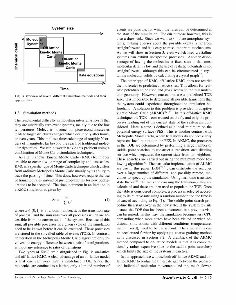
Fig. 3 Overview of several different simulation methods and theirapplicability.

1.3 Simulation methods

The fundamental difficulty in modeling interstellar ices is thatthey are essentially rare-event systems, mainly due to the lowtemperatures. Molecular movement on picosecond timescalesleads to larger structural changes which occur only after hours,or even years. This implies a timescale range of roughly 20 or-ders of magnitude, far beyond the reach of traditional molec-ular dynamics. We can however tackle this problem using acombination of Monte Carlo simulation techniques.

As Fig. 3 shows, kinetic Monte Carlo (KMC) techniquesare able to cover a wide range of complexity and timescales.KMC is a specific type of Monte Carlo technique which differsfrom ordinary Metropolis Monte Carlo mainly by its ability totrace the passing of time. This does, however, require the useof transition rates instead of just probabilities for new config-urations to be accepted. The time increment in an iteration ina KMC simulation is given by

∆t =− lnx∑i ki

, (1)

where x ∈ (0,1] is a random number, ki is the transition rateof process i and the sum runs over all processes which are ac-cessible from the current state of the system. Because of thissum, all possible processes in a given cycle of the simulationneed to be known before it can be executed. These processesare stored in the so-called table of events (TOE). In contrast,an iteration in the Metropolis Monte Carlo algorithm only in-volves the energy difference between a pair of configurations,without any reference to rates of transitions.

Two types of KMC are distinguished in Fig. 3: on-latticeand off-lattice KMC. A clear advantage of an on-lattice modelis that one can work with a predefined TOE. Since themolecules are confined to a lattice, only a limited number of

events are possible, for which the rates can be determined atthe start of the simulation. For our purpose however, this isalso a drawback. Since we want to simulate amorphous sys-tems, making guesses about the possible events is far fromstraightforward and it is easy to miss important mechanisms.As we will show in Section 3, even well-defined crystallinesystems can exhibit unexpected processes. Another disad-vantage of having the molecules at fixed sites is that mostmolecular detail is lost and the use of realistic potentials is notstraightforward; although this can be circumvented in crys-talline molecular solids by calculating a crystal graph26.

The other type of KMC, off-lattice KMC, does not restrictthe molecules to predefined lattice sites. This allows for real-istic potentials to be used and gives access to the full molec-ular geometry. However, one cannot use a predefined TOEsince it is impossible to determine all possible transitions thatthe system could experience throughout the simulation be-forehand. A solution to this problem is provided in adaptivekinetic Monte Carlo (AKMC)27–29. In this off-lattice KMCtechnique, the TOE is constructed on the fly and only the pro-cesses leading out of the current state of the system are con-sidered. Here, a state is defined as a local minimum on thepotential energy surface (PES). This is another contrast withMetropolis Monte Carlo, where trial moves do not necessarilyrepresent local minima on the PES. In AKMC, the processesin the TOE are determined by performing a large number ofsaddle point searches to construct a transition state dividingsurface which separates the current state from its neighbors.These searches are carried out using the minimum mode fol-lowing algorithm30. The particular implementation of AKMCwe use in this paper, EON28,31, can distribute the searchesover a large number of different, and possibly remote, ma-chines to speed up the simulation. Using harmonic transitionstate theory32, the rates for crossing the transition states arecalculated and these are then used to populate the TOE. Oncethe table is considered complete, a process is selected accord-ing to its relative rate using a random number and the time isadvanced according to Eq. (1). The saddle point search pro-cedure then starts over in the new state. If the system revisitsa state, the TOE that has been constructed in a previous visitcan be reused. In this way, the simulation becomes less CPUdemanding when more states have been visited or when ad-ditional simulations, with different conditions (temperature,random seed), need to be carried out. The simulations canbe accelerated further by applying a coarse graining methodas is discussed in Section 3.2. A drawback of the AKMCmethod compared to on-lattice models is that it is computa-tionally rather expensive (due to the saddle point searches)which limits the size of the systems it can treat.

In our approach, we will use both off-lattice AKMC and on-lattice KMC to bridge the timescale gap between the picosec-ond individual molecular movements and the, much slower,

1–10 | 3

timescale for restructuring effects. The AKMC method is par-ticularly useful for simulating complex, rare-event systems,where the kinetic molecular processes are often non-intuitive.On-lattice KMC, on the other hand, has proved its worth whensimulating large systems over long timescales18,25,33,34; butthe TOE needs to be determined beforehand. Our strategy istherefore to use AKMC for determining which typical kind ofprocesses form the crucial transition steps and then translatethis data into an on-lattice model. This approach should beable to really mimic laboratory experiments accurately, cover-ing hours of simulation time.

Since on-lattice KMC has been used for the simulation ofmixed icy layers before, we will focus on the application ofAKMC to molecular systems in the remainder of this paper.

2 AKMC method for molecular systems

Adaptive kinetic Monte Carlo has been demonstrated to workefficiently for atomic systems27,35,36. For the simulation ofinterstellar ices however, we need to progress to molecularsolids. Here, the main complication arises due to the presenceof both strong intramolecular forces and much weaker inter-molecular forces. As a consequence, the PES becomes muchcomplex than that of an atomic system. This makes it harderto locate saddle points using the minimum mode following al-gorithm since the lowest energy eigenvector will vary rapidlywith only small variations in the atomic coordinates.

To demonstrate the suitability of the AKMC method forlong timescale simulation of molecular solids, we apply it hereto a system consisting of an ice Ih(0001) substrate with a singleCO admolecule. The paths generated for the CO molecule areused to compute surface diffusion constants at astronomicallyrelevant temperatures reaching down to 10 K. All simulationswere performed using the EON28,31 software package.

2.1 Potentials

All interactions in the system are described by classical pairpotentials. Molecules are treated as fully flexible, with in-tramolecular forcefields restraining bond lengths and angles.Since our system contains multiple H2O, and a single COmolecule, we need two forcefields. One for H2O-H2O, andanother for the H2O-CO interactions.

Interactions between water molecules are described by theTIP4P/Ice potential37 which has been specifically fitted to re-produce properties of the solid phases of H2O. Intramolecu-lar interactions within the water molecules are treated by thequartic potential proposed by Carney et al.38 (CCL).

The H2O-CO potential was fitted to CCSD(T) (aug-cc-pVTZ, BSSE corrected) calculations of the two-moleculecomplex. For reasons of consistency and computational ef-ficiency, the charges on the H2O molecules are identical to

the TIP4P/Ice charges. CO molecules are modeled with threecharged sites, one on each atom and a third one on the centerof mass. The charges on the atoms depend on the bond lengthin the molecule through the relation:

qi = q0i exp

{−σi

(rCO− r0

CO)}

(i = C,O), (2)

where q0i is the charge in equilibrium configuration, rCO is

the instantaneous bond length and r0CO is the equilibrium bond

length. The third charge is such that the molecule has zerocharge. This model was proposed in order to reproduce thedipole and quadrupole moments from CI (aug-cc-pVTZ) cal-culations39. In addition to the electrostatics, a Buckinghampotential is applied to each atomic intermolecular pair:

UBuckingham(r) = Aexp(−Br)− Cr6 . (3)

Intramolecular interactions within each CO molecule are de-scribed by a Morse potential:

UMorse(rCO) = De[1− exp

{γ(rCO− r0

CO)}]2

. (4)

Experimental values of De and r0CO, which agree to within

0.1% with CCSD(T) (aug-cc-pVQZ) calculations, were usedfor this potential40–42The parameter γ was then fitted to repro-duce the bond length dependence from the ab-initio calcula-tions39. The values of all parameters of the H2O-CO potentialare listed in Table 1.

All interactions are switched off between 9 and 10 A (cen-ter of mass distance between a pair of molecules) using thefunction f (x) = (2x− 3)x2 + 1 with x ∈ (0,1). Ewald sum-mation is not applied for the calculation of long range electro-statics. One argument for this is that during the saddle pointsearches, significant motion of atoms is confined to a finite re-gion around the admolecule, and changes in energy will there-fore be dominated by short-range electrostatics. Furthermore,the restriction to (effective) pair potentials and the ignored po-larizability is likely to have a more severe effect on the energybarriers than the less accurate treatment of the Coulombic in-teractions.

2.2 Simulation details

To initialize a saddle point search, the system is slightly dis-placed from its current configuration in a minimum of thePES. It is known for atomic systems that a Gaussian displace-ment of atoms in the region of interest yields the highest ef-ficiency in finding the low-lying saddle points leading out ofthe initial basin in the PES43. In our simulations however,molecules are displaced instead of atoms. This is done bya translation of the molecule along the three Euclidean axes,followed by a rotation about each axis. Magnitudes of the

4 | 1–10

Table 1 Parameters for the H2O-CO potential

H2O-CO Buckingham parametersInteraction A (eV) B (A−1) C (eVA6)O-C 427.9 2.725 70.38O-O 6.867 ×107 8.022 1.890H-C 667.2 4.506 1.942H-O 537.7 4.551 1.290 ×10−3

CO intramolecular parametersr0

CO 1.128 A σC 3.844 A−1

q0C -0.470 e σO 2.132 A−1

q0O -0.615 e De 11.23 eV

γ 2.328 A−1

displacements and angles of rotation are drawn from Gaus-sian distributions with predefined standard deviation. This ap-proach ensures that the internal geometry of the molecules re-mains unchanged.

The initial displacement starts with the selection of amolecule of interest: the admolecule. Next, a choice is madebetween a single molecule displacement (40% probability)and a multiple-molecule displacement of all molecules whichhave at least one atom within a 4 A radius any atom of the ad-molecule (60% probability). In the case of a single moleculedisplacement, the standard deviation is 0.6 A for displace-ments and 0.5 radians for rotations. For multiple-moleculedisplacements, these standard deviations are 0.3 A and 0.4radians, respectively.

The saddle point searches are conducted using the mini-mum mode following method30, using the Lanczos algorithmto estimate the lowest eigenvector of the Hessian44. Despitethe presence of both intra- and intermolecular forces, testsshow that the saddle point searches have a success rate of ap-proximately 60% in finding a saddle point, which shows thatthe algorithm is rather robust and can be applied to molec-ular systems. The system is considered to be converged ona saddle point when the Hessian has one negative eigenvalueand the force on any atom is below 10−3 eV/A. Minima in thePES are converged to a stricter value of 10−4 eV/A. Any pro-cesses with energy barriers more than 30kT above the lowestbarrier from the state are not included in the TOE since theseare unlikely to be chosen.

An advantage of KMC simulations is that, once the TOEis known for a specific temperature, it is simple to simulateother temperatures. Since the process barriers and prefactorsare temperature independent, one can simply recalculate therates for a new temperature using the harmonic transition statetheory expression32:

k = ν exp(−Eb/kT ), (5)

where ν is the process prefactor and Eb the energy barrier. Byperforming an AKMC simulation at the highest temperature

of interest first, it is then — with the already completed TOE— straightforward to perform additional runs at lower temper-atures.

The ice Ih substrate contains 360 water molecules arrangedin three bilayers. The initial hydrogen bond network is gen-erated using the method of Buch et al.45. It has a negligibledipole moment with periodic boundary conditions applied inall three dimensions. Next, all atomic coordinates are relaxedand the molecules in the bottom bilayer are frozen to mimicbulk ice. The periodic boundary condition along the c-axis isthen removed to create a surface. The CO admolecule is thenadded on the surface and all free coordinates are relaxed again.With this method, we generated three samples with differentproton ordering, which we refer to as samples 1, 2, and 3.

The KMC trajectories give the position of the CO ad-molecule, rrr, on the surface as a function of time. This allowsus to extract the diffusion constants, D, using the Einstein-Smoluchowski equation for two-dimensional diffusion:

D = limt→∞

14t〈|rrr(0)− rrr(t)|2〉. (6)

3 Results

3.1 Binding energies and process barriers

The PESs of the three samples were explored by performingAKMC simulations at T = 50 K. We found 100, 97 and 97states for samples 1, 2 and 3 respectively. The processes inthe TOEs only involve significant translation and rotation ofthe CO admolecule. This is because the temperature is toolow to allow for reorientations of water molecules in the sub-strate, for which energy barriers are at least 200 meV (about2300 K). As a result, the states which are found remain lim-ited in number and form a closed system at any temperaturebelow T = 50 K. By a closed system we mean a system witha TOE which, regardless of the initial state, does not enter anew state even after taking an arbitrarily large number of KMCsteps. This allows for long KMC runs without having to per-form additional saddle point searches, because no new statesare discovered.

The binding sites on sample 2 are shown in the left panel ofFig. 4. Even though the oxygen atoms in the substrate forma crystal lattice, large differences in admolecule orientationbetween the unit cells in the substrate can be seen. These dif-ferences are due to the proton disorder in the ice. This alreadyshows the importance of having an unbiased method to findminima on the PES.

Typically, the admolecule is either at the center of ahexagon, or on top of one of the water molecules in the lowerhalf of the upper half bilayer of the sample. The orientationof the CO molecule is mainly determined by the configuration

1–10 | 5

Fig. 4 Left panel) illustration of all the binding sites of the CO admolecule on ice Ih substrate 2. Configurations of the same color belong tothe same coarse grained composite state. The maximum size of these composite states was limited to 5 in this case. 95 Of the 97 states werecoarse grained, the remaining two configurations are circled in red; the admolecule has a perpendicular orientation w.r.t. the surface in bothcases. Right panel) binding energy of the CO admolecule on the surface of substrate 2. Only the energies of the minima have been included,the saddle points have been left out. The black dots denote the positions of the oxygen atoms in the upper half bilayer of the substrate. Theblack lines show part of a typical trajectory of the admolecule as it diffuses over the substrate by hopping from state to state. The start and endstates of this trajectory are indicated in the figure.

of nearest neighbor dangling protons pointing out of the sur-face, which can be 0, 1, 2 or 3 in number. The orientation isparallel to the surface if there is at least one nearest neighbordangling proton. Without a dangling proton in the vicinity, thebinding site at the center of a hexagon was found to yield astanding CO molecule, having its orientation parallel to the c-axis in the substrate. Two such configurations were found onsample 2 and have been marked by red circles in Fig. 4. Thesecounterintuitive configurations again stress the importance ofhaving an unbiased algorithm to explore the PES. A similarvariety in binding has been observed in simulations of H2Oadmolecule diffusion on the ice Ih(0001) surface46.

Another noteworthy feature of Fig. 4 is that there are manypairs of states in which the position of the CO molecule isalmost identical, but its orientation is different by about 180degrees. These states are connected to each other by processeswhich flip the molecule. These processes have relatively highenergy barriers (60 meV on average) while the configurationalenergies of the states differ on average by only 5 meV.

Besides the admolecule orientation, also the binding ener-gies are strongly influenced by the proton disorder in the sub-strate, as can be seen in the right panel of Fig. 4. This figureshows the binding energy of the CO molecule in the stateson the surface of sample 2, interpolated to a color map. Theanisotropy of the PES is a clear demonstration of the large in-

fluence of proton disorder on the binding energy. Naturally,the energies of the saddle points in between the binding sites,and the corresponding energy barriers, also show a large vari-ation. This appears in the histogram of energy barriers inFig. 5. Energy barriers for CO diffusion are roughly foundto be between 0 and 75 meV, with a few processes which havehigher barriers. The time-averaged binding energy, averagedover KMC runs on each of the three substrates at T = 50 K is154±4 meV. This value is higher than the experimental valueof 115 meV for the adsorption energy of CO at submonolayercoverage on crystalline water ice, which was determined bytemperature programmed desorption47. A possible explana-tion for this discrepancy is that the model charges on the H2Omolecules do not change with the internal geometry of themolecule. With the CCL intramolecular potential, this leads toan increased dipole moment of the water molecules which, inturn, leads to stronger binding energies of the CO admolecule.An additional effect may be that the dipole moments of thewater molecules at the surface can vary significantly depend-ing on the local arrangement, as was observed in recent DFTcalculations48. Because the Tip4p/Ice potential was designedto reproduce bulk properties, the resulting effect on the bind-ing energy is not taken into account. Both effects however,are present at both the potential energy minima and the sad-dle points, the height of the process barriers, and thereby the

6 | 1–10

Barrier height (meV)

Effective diffusion barrier

All barrierscrossed at T=50 Kcrossed at T=25 Kcrossed at T=10 K

0

20

40

60

80

100

0 20 40 60 80 100 120

Fig. 5 Distribution of process energy barriers for CO diffusion onhexagonal ice. The highest, red, bars represent all processes in thetable of events, irrespective of whether or not the barrier is evercrossed during a KMC run. The other bars show the barriers whichare crossed during a KMC simulation at the specified temperature.The vertical black line shows the effective diffusion barrier of 49.4meV. Energy barriers from all three substrates were included in thedata for this figure.

diffusion rate, remains unaffected. In summary, we expect thelargest error to be on the desorption energy due to the use ofa simple bulk potential and only to a lesser extent to the diffu-sion barriers. The calculated binding energies are significantlylarger than the diffusion barriers. This implies that thermaldesorption will occur on a much longer timescale than surfacediffusion. Consequently, it is no problem that desorption pro-cesses are absent in our TOEs §.

3.2 Coarse graining

A common problem in KMC simulations occurs when tran-sition rates in the TOE vary significantly. In this situation,the simulation may become stuck, crossing low barriers overand over again. To avoid spending CPU cycles on simulat-ing this uninteresting behavior, a coarse graining (CG) algo-rithm49 can be applied, which merges states connected by lowbarriers into composite states.

In our systems, the broad distribution of the energy barriers(see Fig. 5) leads to transition rates which vary over many or-ders of magnitude, especially at low temperatures. This was

§ It turns out that the minimum mode following method does not let the ad-molecule climb up from the surface during the saddle point searches. Eventhough it is, in principle, possible to find a saddle point which lets the ad-molecule desorb, it is unlikely that the system will relax back from the tran-sition state to the exact reactant state where the saddle point search started(which is required for a successful saddle point search). It should be notedthough that it is straightforward to include desorption in the TOEs by hand,should one want to.

100

102

104

106

108

1010

1012

1014

0.02 0.04 0.06 0.08 0.10

50 25 20 15 12.5 10

Spe

ed-u

p fa

ctor

1/T (1/K)

T (K)

No coarse grainingComposite size 5

Composite size 10

0

5

10

15

20

0 0.2 0.4 0.6 0.8 1

MS

D (

103

Å2 )

(time (µs)

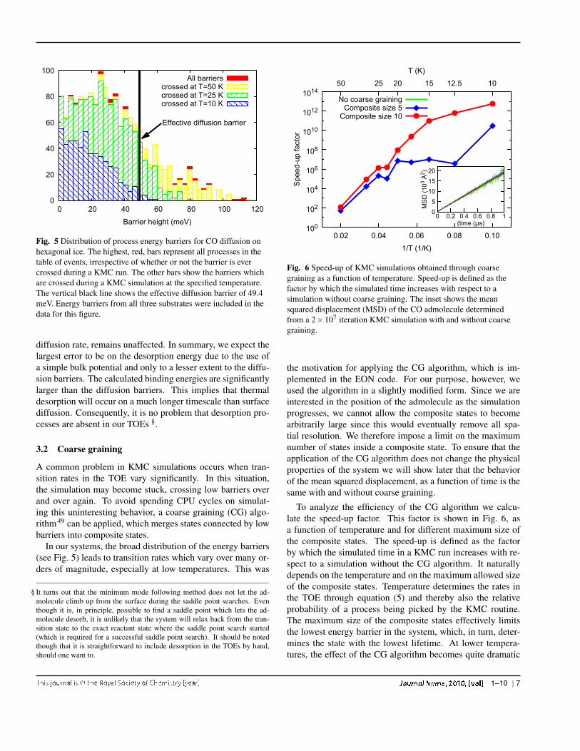
Fig. 6 Speed-up of KMC simulations obtained through coarsegraining as a function of temperature. Speed-up is defined as thefactor by which the simulated time increases with respect to asimulation without coarse graining. The inset shows the meansquared displacement (MSD) of the CO admolecule determinedfrom a 2×107 iteration KMC simulation with and without coarsegraining.

the motivation for applying the CG algorithm, which is im-plemented in the EON code. For our purpose, however, weused the algorithm in a slightly modified form. Since we areinterested in the position of the admolecule as the simulationprogresses, we cannot allow the composite states to becomearbitrarily large since this would eventually remove all spa-tial resolution. We therefore impose a limit on the maximumnumber of states inside a composite state. To ensure that theapplication of the CG algorithm does not change the physicalproperties of the system we will show later that the behaviorof the mean squared displacement, as a function of time is thesame with and without coarse graining.

To analyze the efficiency of the CG algorithm we calcu-late the speed-up factor. This factor is shown in Fig. 6, asa function of temperature and for different maximum size ofthe composite states. The speed-up is defined as the factorby which the simulated time in a KMC run increases with re-spect to a simulation without the CG algorithm. It naturallydepends on the temperature and on the maximum allowed sizeof the composite states. Temperature determines the rates inthe TOE through equation (5) and thereby also the relativeprobability of a process being picked by the KMC routine.The maximum size of the composite states effectively limitsthe lowest energy barrier in the system, which, in turn, deter-mines the state with the lowest lifetime. At lower tempera-tures, the effect of the CG algorithm becomes quite dramatic

1–10 | 7

indeed. For example, at 10 K, a KMC simulation on sample 3had simulated 1.2×109 s and visited 15 of the 97 states after2×107 iterations. With the coarse graining algorithm applied,the simulated time increased by eight orders of magnitude to2.3× 1017 s (comparable to the lifetime of the universe), af-ter which 92 states were visited. Another factor which affectsthe speed-up is the way in which the states are merged intocomposite states. Depending on the initial random seed of thesimulation, different states will be grouped together and somearrangements are more efficient than others. As an example,the color coding in Fig. 4 shows a particular choice of com-posite states on substrate 2.

The time scales reached with the CG algorithm are hugeat low temperatures, even for an interstellar molecular cloud.However, the diffusion constant extracted from the ad-molecule trajectory is still realistic. As is shown in the insetof Fig. 6, the mean squared displacement of the admoleculeas a function of time does indeed not change when the CGalgorithm is applied.

10-30

10-25

10-20

10-15

10-10

10-5

0.02 0.04 0.06 0.08 0.10

50 25 20 15 12.5 10

Diff

usio

n co

nsta

nt (

cm2 /

s)

1/T (1/K)

T (K)

Substrate 1Substrate 2Substrate 3

Fig. 7 Arrhenius plot of the diffusion constants of the COadmolecule on the surface of the three substrates. The lines show thebest fit of an Arrhenius type function through the data points. Thenearly equivalent slopes of the curve show that the effectivediffusion barrier is similar on all three samples.

3.3 Diffusion constants

The surface diffusion constants of the CO admolecule werecalculated from the mean squared displacements in the KMCtrajectories at different temperatures using Eq. (6). In all simu-lations, the CG algorithm was applied with a maximum com-posite state size of 10. At temperatures of 15 K and higher,the admolecule trajectories were found to be sufficiently long

to extract a diffusion constant for all three samples. Despitethe CG algorithm, suitable trajectories at 12.5 K could only beobtained on substrates 1 and 3, and at 10 K only for substrate3. From this we can infer that long, surface-crossing paths,which are accessible at low temperatures, are found most eas-ily on sample 3, whereas these kind of paths are harder to findon samples 1 and 2.

The resulting diffusion constants are shown in Fig. 7. AnArrhenius type behavior is observed, with only slight differ-ences between the three samples. The corresponding energybarriers and pre-exponential factors were extracted from thisdata and are listed in Table 2. The activation energy for diffu-sion is similar for the three samples. It can be interpreted as aneffective diffusion barrier on the substrate, i.e., it is the highestbarrier the admolecule has to cross along the minimum energypath across the surface. The average effective energy barrier isalso shown in Fig. 5, together with the energy barriers whichare crossed at 50, 25 and 10 K. The effective barrier is just atthe end of the range of barriers which are still accessible atT = 10 K. The variation in the pre-exponential factor, D0, islarger. On a perfectly periodic surface, this quantity dependson the process prefactor, the number of processes from eachstate and the hopping distance. In our case, the differencesare likely related to the pattern of dangling protons on the sur-face. Since the dangling protons largely determine the bindingenergies and height of process barriers they dictate which low-energy paths the admolecule can take across the surface. Aswe argued earlier, such paths are most easily found on sub-strate 3. It is therefore not surprising that the pre-exponentialfactor is largest in this sample, since the admolecule can moveabout most easily.

The calculations presented here have assumed the atomscan be described as classical particles. At low temperatureshowever, tunneling will become the dominant transition mech-anism. The AKMC simulation approach can include tunnel-ing as a possible mechanism. From the imaginary frequencyof the unstable mode at each saddle point, an estimate of thecrossover temperature, Tc, for tunneling can be estimated50,and if the temperature of interest is lower than this value, thesaddle point search can be refined to include quantum mechan-ical effects (to converge on so-called instantons). The tran-sition rate is then evaluated from a harmonic quantum TSTrather than a classical harmonic TST51,52. In our simulations

Table 2 Effective diffusion energy barrier and pre-exponential factorD0 for CO diffusion on the three difference ice Ih substrates

Substrate Barrier (meV) D0 (cm2s−1)1 48.6±0.6 (4.08±1.36)×10−2

2 49.5±0.2 (2.76±0.42)×10−2

3 50.3±0.6 (7.94±1.80)×10−2

8 | 1–10

the average Tc was found to be 6±5 K, which justifies the useof the classical approximation.

4 Conclusions

The modeling of interstellar ices still poses a formidable chal-lenge for modern-day simulation techniques. Kinetic MonteCarlo techniques are a powerful tool to study these com-plex systems over long time spans. In this paper we pro-posed a particular approach which combines both on- and off-lattice KMC simulations. Whereas off-lattice KMC simula-tions have demonstrated their use before, off-lattice adaptiveKinetic Monte Carlo has not been used for the simulation ofmolecular systems before. We have demonstrated the poten-tial power of AKMC simulations by performing calculationson a system of a CO admolecule on an hexagonal ice sur-face. Despite the presence of strong intramolecular forces, theminimum-mode following algorithm was able to locate sad-dle points on the PES of the system efficiently to populate theTOE needed for the KMC simulation.

Due to the proton disorder in the ice substrate, the bindingsites of the admolecule were found to show a large variation inboth energy and configuration. This shows that, even for thisrelatively simple system, it is hard to construct a TOE withouthaving an unbiased search algorithm. From the TOE we couldextract information such as the average binding energy andthe height and spread of diffusion energy barriers. Also, typi-cal processes which can occur in the system, like a flip of theCO molecule, could be characterized. These are all examplesof the kind information one would need beforehand when con-structing a TOE for performing on-lattice KMC simulation ofthe same system. This illustrates why the combination of off-lattice AKMC and on-lattice KMC is a potentially very usefulsimulation technique. When combining the two techniqueshowever, one has to be careful when translating the detailedAKMC data into a lattice model. For nearly crystalline sys-tem, as presented in this paper, one should make sure the lat-tice structure represents the crystal structure as much as pos-sible. In this case one would ideally use an hexagonal latticestructure with two sites per lattice point to reproduce the bind-ing sites at the center of a hexagon and those on top of a watermolecule. When dealing with amorphous systems, one shouldchoose a lattice which reproduces the average number of near-est neighbors correctly and make sure that the processes andtheir rates are dependent on the environment (number, kindand possibly orientation of neighbors).

Through the application of a coarse graining algorithm wehave shown that the timescales accessible by AKMC can begreatly enhanced without changing the physical properties ofthe system. This is especially important at low temperatures,where the interesting dynamics takes places on the longesttimescales. From the KMC trajectories we have extracted the

diffusion coefficient for CO on hexagonal ice. From the tem-perature dependence of the diffusion coefficients, the effectivediffusion barrier was determined to be 50±1 meV. The effectof proton disorder of the ice substrate becomes particularlynoticeable at temperatures below 15 K; in this situation theadmolecule can get trapped in certain regions of the surfacemaking large scale movement of the admolecule impossible.

The main conclusion from this work is that we have shownthat AKMC is a promising technique to study kinetic pro-cesses in complex molecular systems like interstellar ices. Itsunbiased saddle point searches, combined with realistic poten-tial energy functions, allow for the identification of transitionmechanisms which one cannot guess beforehand based on in-tuition alone. This unbiased approach is really the power ofAKMC since it gives detailed chemical insight about whichkinetic processes are crucial in the dynamical evolution ofthe ices. However, for the simulation of bulk processes inamorphous ices, the AKMC method is still too expensive tocover astronomically relevant timescales of large systems. Wetherefore believe that using the detailed chemical knowledge,obtainable from AKMC, as input for coarser on-lattice KMCsimulations will be a major step forward in understanding thestructure and dynamics of interstellar ices.

Acknowledgements

This work has been funded by the European Research Coun-cil (ERC-2010-StG, Grant Agreement no. 259510-KISMOL),COST Action Number CM0805 (The Chemical Cosmos: Un-derstanding Chemistry in Astronomical Environments) andthe Icelandic Research Fund administrated by RANNIS. Wegratefully acknowledge M.C. van Hemert for fruitful discus-sions and for providing the CO potential and J.C. Berthet forhelp with the implementation of the water potential in EON.

References1 K. I. Oberg, E. C. Fayolle, H. M. Cuppen, E. F. van Dishoeck and H. Lin-

nartz, Astron. Astrophys., 2009, 505, 183.2 J. T. H. van Eupen, W. W. J. Elffrink, R. Keltjens, P. Bennema,

R. de Gelder, J. M. M. Smits, E. R. H. van Eck, A. P. M. Kentgens, M. A.Deij, H. Meekes and E. Vlieg, Cryst. Growth Des., 2008, 8, 71.

3 J. Los, W. J. P. van Enckevort, H. Meekes and E. Vlieg, J. Phys. Chem. B,2007, 111, 782.

4 A. M. Nienow and J. T. Roberts, Annu. Rev. Phys. Chem., 2006, 57, 105.5 K. Muralidharan, P. Deymier, M. Stimpfl, N. H. de Leeuw and M. J.

Drake, Icarus, 2008, 198, 400.6 D. Bockelee-Morvan, D. C. Lis, J. E. Wink et al., Astron. Astrophys.,

2000, 353, 1101.7 S. Viti, M. P. Collings, J. W. Dever, M. R. S. McCoustra and D. A.

Williams, Mon. Not. R. Astron. Soc., 2004, 354, 1141.8 R. T. Garrod, V. Wakelam and E. Herbst, Astron. Astrophys., 2007, 467,

1103.9 E. Herbst and E. F. van Dishoeck, Annu. Rev. Astron. Astr., 2009, 47, 427.

1–10 | 9

10 E. L. Gibb, D. C. B. Whittet, A. C. A. Boogert and A. G. G. M. Tielens,Astrophys. J. Suppl. S., 2004, 151, 35.

11 A. C. A. Boogert, K. M. Pontoppidan, C. Knez et al., Astrophys. J., 2008,678, 985.

12 H. M. Cuppen, E. M. Penteado, K. Isokoski, N. van der Marel and H. Lin-nartz, Mon. Not. R. Astron. Soc., 2011, 417, 2809.

13 K. M. Pontoppidan, A. C. A. Boogert, H. J. Fraser, E. F. van Dishoeck,G. A. Blake, F. Lahuis, K. I. Oberg, N. J. Evans, II and C. Salyk, Astro-phys. J., 2008, 678, 1005.

14 P. Caselli, T. I. Hasegawa and E. Herbst, Astrophys. J., 1993, 408, 548.15 R. T. Garrod, S. L. W. Weaver and E. Herbst, Astrophys. J., 2008, 682,

283.16 A. I. Vasyunin, D. A. Semenov, D. S. Wiebe and T. Henning, Astrophys.

J., 2009, 691, 1459.17 M. P. Collings, M. A. Anderson, R. Chen, J. W. Dever, S. Viti, D. A.

Williams and M. R. S. McCoustra, Mon. Not. R. Astron. Soc., 2004, 354,1133.

18 H. M. Cuppen, E. F. van Dishoeck, E. Herbst and A. G. G. M. Tielens,Astron. Astrophys., 2009, 508, 275.

19 A. G. G. M. Tielens and W. Hagen, Astron. Astrophys., 1982, 114, 245.20 T. I. Hasegawa, E. Herbst and C. M. Leung, Astrophys. J. Suppl. S., 1992,

82, 167.21 P. Caselli, T. I. Hasegawa and E. Herbst, Astrophys. J., 1998, 495, 309.22 S. Ioppolo, H. M. Cuppen, C. Romanzin, E. F. van Dishoeck and H. Lin-

nartz, Astrophys. J., 2008, 686, 1474.23 G. W. Fuchs, H. M. Cuppen, S. Ioppolo, C. Romanzin, S. E. Bisschop,

S. Andersson, E. F. van Dishoeck and H. Linnartz, Astron. Astrophys.,2009, 505, 629.

24 B. Barzel and O. Biham, Astrophys. J. Lett., 2007, 658, 37.25 H. M. Cuppen and E. Herbst, Astrophys. J., 2007, 668, 294.26 S. X. M. Boerrigter, G. P. H. Josten, J. van de Streek, F. F. A. Hollander,

J. Los, H. M. Cuppen, P. Bennema and H. Meekes, J. Phys. Chem. A,2004, 108, 5894–5902.

27 G. Henkelman and H. Jonsson, J. Chem. Phys., 2001, 115, 9657.28 A. Pedersen and H. Jonsson, Math. Comput. Simulat., 2010, 80, 1487.29 H. Jonsson, Proc. Natl. Acad. Sci. USA, 2011, 108, 944.30 G. Henkelman and H. Jonsson, J. Chem. Phys., 1999, 111, 7010.31 http://www.theochem.org/EON.32 H. Vineyard, J. Phys. Chem. Solids, 1957, 3, 121.33 K. I. Oberg, E. C. Fayolle, H. M. Cuppen, E. F. van Dishoeck and H. Lin-

nartz, Astron. Astrophys., 2009, 505, 183.34 S. Cazaux, V. Cobut, M. Marseille, M. Spaans and P. Caselli, Astron.

Astrophys., 2010, 522, A74.35 A. Pedersen and H. Jonsson, Acta Material., 2009, 57, 4036.36 A. Pedersen, G. Henkelman, J. Schiøtz and H. Jonsson, New J. Phys.,

2009, 11, 073034.37 J. L. F. Abascal, E. Sanz, R. Garcıa Fernandez and C. Vega, J. Chem.

Phys., 2005, 122, 234511.38 S. K. Langhoff, L. A. Curtiss and G. Carney, J. Mol. Spectrosc., 1976, 61,

371.39 M. C. van Hemert, Private Communication, 2011.40 A. Mantz and J. Maillard, J. Mol. Spectrosc., 1975, 57, 155.41 V. I. Vedeneyev, L. V. Gurvich, V. N. Kondratyev, V. A. Medvedev

and Y. L. Frankevich, Bond Energies, Ionization Potentials and ElectronAffinities, St. Martin’s Press, New York, 1962.

42 P. Bunker, J. Mol. Spectrosc., 1972, 5, 478.43 A. Pedersen, S. F. Hafstein and H. Jonsson, Siam. J. Sci. Comput., 2011,

33, 633.44 R. Malek and N. Mousseau, Phys. Rev. E, 2000, 62, 7723.45 V. Buch, P. Sandler and J. Sadlej, J. Phys. Chem. B, 1998, 102, 8641.46 E. Batista and H. Jonsson, Comp. Mater. Sci., 2001, 20, 325.

47 J. A. Noble, E. Congiu, F. Dulieu and H. J. Fraser, Mon. Not. R. Astron.Soc., 2012, 421, 768.

48 M. Watkins, D. Pan, E. G. Wang, a. Michaelides, J. VandeVondele andB. Slater, Nat. Mat., 2011, 10, 794.

49 A. Pedersen, J. C. Berthet and H. Jonsson, Lect. Notes. Comput. Sc., 2012,7134, 34.

50 M. Gillan, J. Phys. C Solid State, 1987, 20, 3621.51 G. Mills, G. K. Schenter, D. E. Makarov and H. Jonsson, Chem. Phys.

Lett., 1997, 278, 91.52 S. Andersson, G. Nyman, A. Arnaldsson, U. Manthe and H. Jonsson, J.

Phys. Chem. A, 2009, 113, 4468.

10 | 1–10