long-term skewness and systemic risk - · pdf filelong-term skewness and systemic risk ......

Journal of Financial Econometrics, 2011, Vol. 9, No. 3, 437–468

Long-Term Skewness and Systemic RiskROBERT F. ENGLE

Stern School of Business at New York University

ABSTRACTFinancial risk management has generally focused on short-term risksrather than long-term risks, and arguably this was an importantcomponent of the recent financial crisis. Econometric approaches tomeasuring long-term risk are developed in order to estimate the termstructure of value at risk and expected shortfall. Long-term negativeskewness increases the downside risk and is a consequence of asym-metric volatility models. A test is developed for long-term skewness. Ina Merton style structural default model, bankruptcies are accompaniedby substantial drops in equity prices. Thus, skewness in a market factorimplies high defaults and default correlations even far in the future cor-roborating the systemic importance of long-term skewness. Investorsconcerned about long-term risks may hedge exposure as in the In-tertemporal Capital Asset Pricing Model (ICAPM). As a consequence,the aggregate wealth portfolio should have asymmetric volatility andhedge portfolios should have reversed asymmetric volatility. Using es-timates from VLAB, reversed asymmetric volatility is found for manypossible hedge portfolios such as volatility products, long- and short-term treasuries, some exchange rates, and gold. ( JEL: G01)

KEYWORDS: ARCH, GARCH, Hedge portfolios, long-term risk, ICAPM,skewness, systemic risk

The financial crisis that engulfed the global economy in 2008 and 2009 has beendescribed and diagnosed by many. A thoughtful discussion of the causes andremedies can be found in Acharya and Richardson (2009), Acharya et al. (2010),or Brunnermeier et al. (2009) in the Geneva Report. While there are many complexunderlying causes, there are two key features of all analyses. First is the failure ofmany risk management systems to accurately assess the risks of financial positions,

Address to correspondence to Robert F. Engle, Stern Schoolf of Business at New York University,44 West Fourth Street, New York, NY 0012, or e-mail: [email protected].

doi: 10.1093/jjfinec/nbr002c© The Author 2011. Published by Oxford University Press. All rights reserved.

For permissions, please e-mail: [email protected].

at New

York U

niversity on Septem

ber 20, 2011jfec.oxfordjournals.org

Dow

nloaded from

http://jfec.oxfordjournals.org/

438 Journal of Financial Econometrics

and the second is the failure of economic agents to respond appropriately to theserisks. The explanations for the failure to act are based on distorted incentives due toinstitutional structures, compensation practices, government guarantees, and reg-ulatory requirements. In short, many agents were paid well to ignore these risks.These two features are inextricably linked, and it is unlikely that we will be able toquantify the relative importance of miss-measurement of risk from the incentivesto ignore risk. The wide-ranging legislative approach to reregulating the financialsector is designed to reduce the mismatch of incentives. This includes systemicrisks, “too big to fail” firms, counterparty risks in Over the Counter (OTC) deriva-tives markets, government bank deposit guarantees as a distorting factor in pro-prietary trading, and many other institutional features.

In this paper, I would like to focus primarily on the question of whether riskswere then or are now being measured appropriately. Was this financial crisis fore-cast by risk managers? Was this crisis in a 99% confidence set of possible outcomes?Was there economic or econometric information available that was not being usedin risk assessment and how could risk management systems be augmented to takesuch factors into account?

In approaching this question, I will examine the performance of simple riskmeasurement systems that are widely used but will not attempt to document whatwas in place at what institution. The most widely used measure and one that hasbeen frequently criticized is the value at risk (VaR) of a firm or portfolio. This isthe 1% quantile of the distribution of future values and is typically defined overthe next trading day. A preferable number for theoretical reasons is the expectedshortfall or the loss that is expected to occur if the VaR is exceeded. Both of thesemeasures are based on a volatility forecast, and it is natural to examine the accu-racy of volatility forecasts in this economic environment.

Each of these measures is defined over a 1-day horizon. In some cases, longerhorizons are used such as a 10-day horizon, but the risk measures for these longerhorizons are simply scaled up on the assumption that the risk is constant. Forexample, the 10-day VaR is typically computed as the square root of 10 timesthe 1-day VaR. Both measures require statistical assumptions in order to estimateand forecast risk. The precision and stability of the measures depends upon themethodology being used.

A recent study, Brownlees, Engle, and Kelly (2009), has examined the real-timeforecasting performance of volatility models for a variety of different methodsand assets. These are daily models based on a range of asymmetric GeneralizedAutoregressive Conditional Heteroskedasticity (GARCH) models reestimated pe-riodically. The surprising finding is that these models showed almost no deteriora-tion during the financial crisis. Using a statistical loss function, volatility forecastswere just as accurate during the crisis as before it, and risk management basedon these forecasts was also robust to the crisis. This finding appears in conflictwith the quoted observation that risk managers underestimated risk. The impor-tant issue is that both volatility forecasting and calculations of VaR and ES arecomputed as 1 day ahead forecasts. The financial crisis was predictable one day ahead.

at New

York U

niversity on Septem


Dow

nloaded from


ENGLE | Long-Term Skewness and Systemic Risk 439

It is immediately clear that this is not enough notice for managers who invest inilliquid assets such as the mortgage backed securities at the center of the crisis.Risk management must give more warning if it is be useful.

The short-run nature of VaR, and ES is a very important feature. Positionsheld for more than one day will have additional risk due to the fact that risk itselfcan change. Engle (2009b) describes this as the “risk that the risk will change.”Most investors and financial firms hold positions much longer than one day andconsequently, changes in risk will be a very important determinant of returns. Amarket timing approach to the holding period of assets might attempt to closepositions before the risk increases, but this is bound to be unsuccessful for theaverage investor.

Consider the situation prior to this crisis. From 2003 until mid 2007, volatil-ities were very low, and from 2002 until mid 2004, short-term interest rates werevery low. Thus, highly leveraged positions in a wide range of securities had lowshort-term risk. Many financial institutions everywhere in the globe took on thesepositions, but when volatilities and interest rates rose, the value of the positionsfell dramatically precipitating the financial crisis. Many economists and analystsviewed the rise in interest rates and volatility as likely and the options market andfixed income market certainly forecast rises, yet our simple risk measures did nothave a way to incorporate these predictions. Thus, an important challenge to riskassessment is to develop measures that can capture both short- and long-term risk.

In the next section, a term structure of risk will be estimated for various volatil-ity models. Section 4 will develop a test for long-term skewness to see if standardvolatility models are capable of modeling this characteristic of the data and the riskit generates. In Section 5, the economic underpinning of the asymmetric volatilitymodels is developed along the lines first suggested by French, Schwert, and Stam-baugh (1987). Section 6 extends this logic to hedge portfolios as in the Merton(1973) ICAPM. These hedge portfolios provide a solution to asset allocation withchanging state variables. It is argued that this solution would reduce the systemicrisk of the financial system if it were widely adopted.

1 TERM STRUCTURE OF RISK

To reflect the variety of investment horizons available to financial firms, this paperwill follow Guidolin and Timmermann (2006) and define a term structure of riskwhich is a natural analogy with the term structure of interest rates and the termstructure of volatility. Risk measures are computed for horizons from one day tomany years which illustrate both short- and long-term risks. The measures are de-fined to consider the losses that would result from extreme moves in underlyingasset prices over these different horizons. Major risks that will take time to unfoldwill lead to high long-term risks relative to short-term risks.

There are some conceptual issues in defining such risks, but the serious chal-lenge is how to measure them. The ultimate goal is to choose investment strategiesthat are optimal in the face of such term structures of risk.

at New

York U

niversity on Septem


Dow

nloaded from



If the value of a portfolio at time t is St and its log is st, then the loss is thedifference between the date T value and the current value. Hence, the VaR at levelalpha and horizon T per dollar invested is given by

Pt(St+T/St − 1 < −VaRα,T) = α. (1)

Equivalently,

Pt(st+T − st < log(1−VaRα,T)) = α. (2)

The evaluation of this expression requires a model of the distribution of this assetat time t+T. Because this expression reflects the distribution of returns, it incorpo-rates information on both expected returns and deviations from expected returns.For short horizons, it does not matter whether expected returns are considered ornot but for longer horizons, this distinction is very important. After all, if expectedreturns are positive then long horizon returns will be proportional to T and sincevolatility is proportional to the square root of T, ultimately for sufficiently large T,VaR will be negative.

A variation on traditional VaR will be used here to separate forecasts of riskand return. VaR0 will be defined as the α quantile of losses assuming expectedcontinuously compounded returns are zero. Expected losses from holding the assettherefore can be estimated without a model of expected returns. This definitionbecomes

Pt(st+T − Etst+T < log(1−VaR0α,T)) = α. (3)

Consequently, the relation between the two measures of VaR is approximately

VaRα,T ∼= VaR0α,T − μT, (4)

where μ is the expected return. Clearly, the larger the estimate of μ, the less riskythe asset appears thereby confounding the separate estimation of risk and return.Since riskier assets will generally have higher expected returns, the measure ofrisk and return should be constructed separately and then combined in portfoliochoice.

Measures based on VaR are widely criticized from at least two additionalpoints of view. The first is theoretical in that this measure is not coherent in thesense that it does not satisfy natural axioms of diversification. The second criticismis that by ignoring the size of the risk in the alpha tail, VaR encourages traders totake positions that have small returns almost always and massive losses a tiny frac-tion of the time. A measure designed to correct these flaws is ES which is definedas the expected loss should VaR be exceeded. Hence,

ESα,T = −Et(St+T/St − 1|St+T/St < 1−VaRα,T) (5)

at New

York U

niversity on Septem


Dow

nloaded from



and

ES0α,T= −E0

t (St+T/St − 1|St+T/St < 1−VaR0α,T). (6)

Again the superscript 0 refers to the assumption that the mean logarithmic returnis zero. The advantage of ES is also its disadvantage—it is difficult to estimate thelosses in the extreme tail of the distribution.

An approach to estimating these losses is to use extreme value theory. In thisapproach, the tails of the distribution have the shape of a Pareto or Frechet dis-tribution regardless of the underlying distribution within a wide and reasonableclass of distributions. Only one parameter is required in order to have an estimateof the probability of extremes even beyond any that have been experienced. ThePareto distribution is defined by

F(x) = 1− (x/x0)−λ, x � x0 > 0. (7)

The larger the parameter λ, the thinner the tails of the distribution. As well known,x has finite moments only for powers strictly smaller than λ, see, for example, Mc-Neil, Embrechts, and Frey (2005). The tail parameter of the student-t distributionis its degrees of freedom. The Pareto density function is

f (x) = λ(x/x0)−λ−1/x0, x > x0 > 0. (8)

And the mean of x, given that it exceeds the threshold, is given by

E(x|x > x0) =λx0

λ− 1, λ > 1. (9)

The estimation of tail parameters is done on losses not on log returns. Thus x isinterpreted as

xt = 1− St+T/St (10)

Assuming that the tail beyond VaR is of the Pareto form and recognizing that itcan directly be applied to the lower tail by focusing on losses as in Equation (10),an expression for the expected shortfall is simply

ES0α,T= VaR0

α,T

(λ

λ− 1

). (11)

A common approach to estimating λ is the Hill estimator. See McNeil, Embrechts,and Frey (2005). This strategy defines a truncation point x0 such that all data ex-ceeding this value are considered to be from a Pareto distribution. These observa-tions are used to form a maximum likelihood estimator (MLE) of the unknown tail

at New

York U

niversity on Septem


Dow

nloaded from



parameter. Assuming all losses exceeding VaR follow such a Pareto distribution,the Hill estimator is

λ̂ =

∑t∈Exceed

1

∑t∈Exceed

log(zt), zt =

1− ST+t/St

VaR0α,T

. (12)

It has been shown that under some regularity conditions, see Resnick and Starica(1995), and references therein, Hill’s estimator is still consistent for the tail indexof the marginal distribution in a time series context if this marginal distribution isassumed to be time invariant.

2 ESTIMATING THE TERM STRUCTURE OF RISK

In order to estimate these measures for a real data set at a point in time, a simula-tion methodology is natural. This of course requires a model of how risk evolvesover time. A familiar class of models is the set of volatility models. These mod-els are empirically quite reliable and find new applications daily. However, theydo not have a rigorous economic underpinning although some steps along thispath will be discussed later in this paper. Each volatility model could be the data-generating process for the long-term risk calculation. For a recent analysis of theforecasting performance of these volatility models during the financial crisis, seeBrownlees, Engle, and Kelly (2009).

The simulation methodology can be illustrated for the simple GARCH(1,1)with the following two equations:

rt =√

htεt,ht+1 = ω+ (αε2

t + β)ht.(13)

These equations generate returns, r, as the product of the forecast standard devi-ation and an innovation that is independent over time. The next day conditionalvariance also depends on this innovation and forecast standard deviation. Thus,the random shock affects not only returns but also future volatilities. From a timeseries of innovations, this model generates a time series of returns that incorpo-rates the feature that volatility and risk can change over time. The distributionof returns on date T incorporates the risk that risk will change. Two simulationswill be undertaken for each model, one assumes that the innovations are stan-dard normal random variables, and the other assumes that they are independentdraws from the historical distribution of returns divided by conditional standarddeviations and normalized to have mean zero and variance one. This is called thebootstrap simulation. It is also called the Filtered Historical Simulation (FHS) byBarone-Adesi, Engle, and Mancini (2008).

A collection of asymmetric volatility processes will be examined in this pa-per but the list is much longer than this and possibly the analysis given below

at New

York U

niversity on Septem


Dow

nloaded from



will suggest new and improved models. See, for example, Bollerslev (2008) for acomprehensive list of models and acronyms.

TARCH : ht+1 = ω+ αr2t + γr2

t Irt<0 + βht,

EGARCH : log(ht+1) = ω+ α|εt|+ γεt + β log(ht), εt = rt/√

ht,

APARCH : hδ/2t+1 = ω+ α(|rt| − γrt)δ + βhδ/2

t ,

NGARCH : ht+1 = ω+ α(rt − γ√

ht)2 + βht,

ASQGARCH : ht+1 = ω+ βht + (α(r2t − ht) + γ(r2

t Irt<0 − ht/2))h−1/2t .

(14)

Each of these models can be used in place of the second equation of (13).In the calculations below, parameters are estimated using data on S&P500 re-

turns from 1990 to a specified date. These parameter estimates and the associateddistribution of standardized returns are used to simulate 10,000 independent sam-ple paths 4 years or 1000 days into the future. For each of these horizons, the riskmeasures described above are computed.

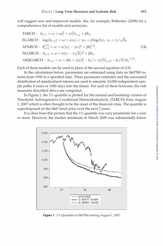
In Figure 1, the 1% quantile is plotted for the normal and bootstrap version ofThreshold Autoregressive Conditional Heteroskedasticity (TARCH) from August1, 2007 which is often thought to be the onset of the financial crisis. The quantile issuperimposed on the S&P stock price over the next 2 years.

It is clear from this picture that the 1% quantile was very pessimistic for a yearor more. However, the market minimum in March 2009 was substantially below

Figure 1 1% Quantiles of S&P500 starting August 1, 2007.

at New

York U

niversity on Septem


Dow

nloaded from



the simulation based on normal errors and approximately equal to the bootstrapsimulation of the TARCH. The probabilistic statement here should be taken care-fully. These bands have the property that at any horizon, the probability of exceed-ing the band is 1%. This does not mean that the probability of crossing the bandsomewhere is 1%, presumably it is substantially greater. Furthermore, by choosingthe very beginning of the crisis as the starting point, I am again being nonrandomin the choice of which curves to present.

In Figure 2, the same quantiles are plotted from three other starting points,January 2008, September 2008, and June 2009, the end of the sample.

Clearly, the quantile starting in September 2008 just before the Lehmanbankruptcy was quickly crossed. Now in 2010, it appears that the quantile startingin June will not be crossed at all but perhaps we should wait to see.

In comparison, several other quantile estimates are computed. Particularly in-teresting are the quantiles when returns are independent over time. Also com-puted are quantiles from EGARCH and APARCH models. These are shown inFigure 3 clustered between the TARCH and the i.i.d. quantiles.

The quantiles for i.i.d. shocks show far less risk than all the other models andthey do not depend upon whether the shocks are normal or bootstrapped. Thequantiles for the EGARCH and APARCH also depend little on whether the shocksare normal or bootstrapped. In fact, these models perform rather similarly.

For each of these simulations and for each horizon, the ES can be estimatedempirically and the tail parameter can be estimated by the Hill estimator thusgiving an alternative estimate of the ES using Equation (11).

Figure 2 1% Bootstrap Quantiles from various starting points.

at New

York U

niversity on Septem


Dow

nloaded from



Figure 3 1% Quantiles for TARCH, APARCH, EGARCH, and i.i.d. sampling.

For each method, the tail parameter is estimated for each horizon and ispresented in Figure 4. The smaller the number, the fatter the tail. As can be seen,the tails for all methods become thinner as the horizon increases and the distribu-tion gradually approaches the normal. For the bootstrapped TARCH, the tails aremost extreme. When this parameter drops below four, the fourth moment does notexist. The two i.i.d. methods have distributions that converge with the number ofreplications to normal distributions rather than Frechet, hence, the tail parameteris not well defined and these estimates are presumably not consistent. The othermethods are broadly similar which suggests that the tail parameter can perhaps beinferred from the horizon.

Based on these tail parameters and the quantiles computed above, the ES canbe easily estimated. As the tail parameters should be approximately invariant tothe choice of tail quantile, this provides a measure of ES that can be computed forany probability. These are shown in Figure 5.

Clearly, the highest losses are for the bootstrapped TARCH model and thelowest are for the i.i.d. models. The others are broadly similar.

3 LONG-TERM SKEWNESS

It is now widely recognized that asymmetric volatility models generate multi-period returns with negative skewness even if the innovations are symmetric. This

at New

York U

niversity on Septem


Dow

nloaded from



Figure 4 Tail parameters at different horizons for different models.

Figure 5 ES by horizon and method computed from tail parameter.

at New

York U

niversity on Septem


Dow

nloaded from



argument is perhaps first emphasized by Engle (2004). The explanation is simple.Since negative returns predict higher volatilities than comparable positive returns,the high volatility after negative returns means that the possible market declinesare more extreme than the possible market increases. In Berd, Engle, and Voronov(2007), an expression for unconditional skewness at different horizons is given.Here, a simulation will be used to estimate how skewness varies over horizon.

Skewness is defined in terms of long horizon continuously compounded orlog returns as

skt(T) =Et(st+T − st − μ)3

[Et(st+T − st − μ)2]3/2 , μ = E(st+T − st). (15)

In a simulation context, this is easily estimated at all horizons simply by calculatingthe skewness of log returns across all simulations. This is naturally standardizedfor the mean and standard deviation of the simulation. By using log return, thismeasure focuses on asymmetry of the distribution. A distribution is symmetric ifan x% decline is just as likely as an x% increase for any x% change. Hence, skew-ness is a systematic deviation from symmetry and negative skewness means thatlarge declines are more likely than similar size increases.

For the horizons from 1 to 100 days, Figure 6 presents the results. All theskewness measures are negative and are increasingly negative for longer horizons.The simulations based on the normal distribution start at zero while the measuresbased on the bootstrap start at −0.4. However, after 50 days, the TARCH has fallensubstantially below the other methods. The unconditional skewness of the data onSP500 returns from 1990 to 2009 is also plotted in this graph. This is also stronglynegatively skewed becoming more negative as the term of the return is increased.The striking feature, is that the data are more negatively skewed than any of themodels, at least between 5 and 45 days.

In Figure 7, the same plot is shown for longer horizons. Now, it is clear thatthe bootstrap TARCH is the most negative and the data are the least negative. Itmay also be apparent in the simulation that the bootstrap TARCH is very unstable.Presumably, it does not have finite sixth moments so the skewness is not consis-tently estimated. The other five estimators are rather similar. The most negativeskewness is for approximately 1-year horizon and for still longer horizons, theskewness gradually approaches zero. However, this is extremely slow so that theskewness at a 4-year horizon is still −1.

4 TESTING LONG-TERM SKEWNESS

It is not clear that these models give accurate estimates of skewness of timeaggregated returns. The data appears to be more negatively skewed for short hori-zons and less negatively skewed for long horizons than the models. The mod-els are estimated by maximum likelihood but this focuses on the one step ahead

at New

York U

niversity on Septem


Dow

nloaded from



Figure 6 Skewness of different methods.

Figure 7 Skewness of different methods and horizons.

at New

York U

niversity on Septem


Dow

nloaded from



volatility forecast and may not reveal misspecification at long horizons. In thissection, an econometric test is developed to determine whether the long-termskewness implied by a set of parameter estimates is significantly different fromthat in the data. It is a conditional moment test and has a well-defined asymptoticdistribution. However, because it uses overlapping data and in some cases, highlyoverlapping data, it is unlikely that the asymptotic distribution is a good guideto the finite-sample performance. Thus, Monte Carlo critical values are also com-puted. In brief, it is found that the models cannot be rejected for misspecificationof long-term skewness.

The test is based on the difference between the third moment of data simulatedfrom the model with estimated parameters and the third moment of the data. Fora horizon k and estimated parameters θ̂, the process is simulated N times withbootstrapped innovations to obtain a set of log asset prices{si

k(θ̂)}. The moment tobe tested is therefore

mkt (θ̂) =

(st − st−k − 1

T

T

∑j=k(sj − sj−k)

)3

⎡⎣1

T

T

∑t=k

(st − st−k −

(1T

T

∑j=k(sj − sj−k)

))2⎤⎦

3/2 −1N

N

∑i=1

(si

k(θ̂)− sik(θ̂))3

[1N

N

∑i=1

(si

k(θ̂)− sik(θ̂))2]3/2

(16)

The expected value of this moment should be zero if the model is correctlyspecified and the sample is sufficiently large.

To test whether the average of this moment is zero, a simple outer productof the gradient test can be used with simulated moments. This test approach wasinitially used by Godfrey and Wickens (1981) and formed the core of the Berndtet al. (1974) maximization algorithm , now called BHHH. It was nicely expositedin Davidson and MacKinnon (1993, Chapter 13.7 and 16.8) and Engle (1984). It iswidely used to construct conditional moment tests under the assumption that themoment condition converges uniformly to a normal mean-zero random variablewith a variance that is estimated by its long-run variance.

The test is then created by regressing a vector of 1s on the first derivativematrix of the log likelihood function and the added sample moments.

L(θ) =T

∑t=1

Lt(θ), Gt(θ) ≡ ∂Lt/∂θ′, 1 = G(θ̂)c+M(θ̂)b+ resid, (17)

where M is the matrix of moment conditions from Equation (16). The test statisticis simply the joint test that all the coefficients b = 0.

Because of the dependence between successive moment conditions and poten-tial heteroskedasticity, this distribution theory only applies when Heteroskedas-ticity and Autocorrelation Consistent Covariance (HAC) standard errors are used.

at New

York U

niversity on Septem


Dow

nloaded from



Figure 8 Critical values for long-term skewness test at 2.5% in each tail.

Figure 9 T-statistics for long-term skewness test.

Even with such technology, there is a great deal of experience that suggests that thefinite-sample distribution is not well approximated by the asymptotic distributionwhich is a standard normal. Thus, I will compute Monte Carlo critical values aswell as asymptotic critical values.

The test is done for one horizon k at a time. Parameters are estimated by MLEusing the full sample and then the skewness at horizon k appropriate for theseparameters is computed by simulating 10,000 sample paths of length k. The mo-ment condition (16) can then be constructed for each data point to obtain a vectorof moments M. Equation (17) is estimated by ordinary least squares (OLS) butthe standard errors are constructed to correct for heteroskedasticity and autocor-relation. This is done with prewhitening and then applying Newey West with avariable bandwidth. The standard error associated with b is used to construct at-statistic and this is tested using either the standard normal distribution or theMonte Carlo distribution.

at New

York U

niversity on Septem


Dow

nloaded from



To compute the Monte Carlo critical values, 1000 replications are computedwith a sample size of 2000 and skewness computed in Equation (16) from 10,000bootstrapped simulations. An upper and a lower 2.5% quantile are extracted andused as alternative critical values for the t-statistic. The parameters used for thisMonte Carlo are close approximations to the data-based parameters.

The Monte Carlo critical values for the TARCH and EGARCH correspondingto the upper and lower tails using bootstrapped simulations are rather far from thestandard normal. The critical values are given in the following table:

Thus, the critical values for TARCH models using a horizon of 10 days wouldbe (−2.7,2.8), while for the 500-day horizon, it would be (−0.2, 10). Clearly, theasymptotic (−2,2) is not a very good approximation, particularly, for long horizonswhere the overlap is very large. The EGARCH is more symmetrical and somewhatcloser to the asymptotic distribution at least up to 50 days.

When this test is applied for long time series on the SP500 for the five modelsused in this paper for the five horizons, the t-statistics are given in Figure 9. Noticethat the largest t-statistic is for the 500 day overlap with TARCH. Its value of 5.5exceeds any reasonable approximation to the asymptotic assumption of standardnormality, however, from Figure 8, it is clear that the finite-sample distributionis dramatically skewed and that this value does not exceed the critical value. Noother t-statistics exceed two or exceed the Monte Carlo critical values. Thus, theconclusion is that all these models appear to generate long-term skewness that isconsistent with the SP data.

5 LONG-TERM SKEWNESS AND DEFAULT CORRELATIONS

In a Merton style model of default, the probability of default is the probabilitythat the equity price will fall below a default threshold. The location of the de-fault threshold can be estimated from the probability of default which is pricedin the market for credit default swaps. In simple models designed to measurethe frequency of defaults over a time period, it is often assumed that all firmsare identical. Consequently, all firms must have the same market beta, idiosyn-cratic volatility, probability of default, and default threshold. The data-generatingprocess is simply the one factor model

ri,t = rm,t + σiεi,t. (18)

The distribution of defaults depends only on the properties of market returns andidiosyncratic returns. When the market return is positive, there are only defaultsfor companies with large negative idiosyncratic returns. When the market return isvery negative, there are defaults for all companies except the ones with very largepositive idiosyncrasies. The probability of default is the same for all companies,but it is much more likely for some simulations than for others. This model isdeveloped in more detail in Berd, Engle, and Voronov (2007).

at New

York U

niversity on Septem


Dow

nloaded from



For normal and constant volatility idiosyncracies and defaults that occurwhenever the stock price is below the default threshold at the end of the period,the probability of default is given by

πi = π = P(ri,t < kt) = E[P(ri,t < kt|rm,t)]

= E[P(εi < (kt − rm,t)/σi|rm,t)]

= E[Φ((kt − rm,t)/σi)].

(19)

The value of k each period is chosen to satisfy Equation (19) for a set of simulationsof market returns. The default correlation is defined as the correlation betweenindicators of default for any pair of companies. It is the covariance between theseindicators divided by the variance. This can be estimated using the independencebetween idiosyncrasies using the following expression:

ρdt = (P(ri,t < kt & rj,t < kt)− π2)/(π − π2)

= (E[Φ((kt − rm,t)/σ)2|rm,t]− π2)/(π − π2)

= (V[Φ((kt − rm,t)/σ)])/(π − π2).

(20)

Assuming the annual probability of default is 1%, the default frontier can be eval-uated for different models by solving Equation (19) for k. Then the number of de-faults calculated for any simulation. Idiosyncratic volatility is assumed to be 40%so the average correlation of two names is 18%. In Figure 10, the number of de-faults that occur on the 1% worst case simulation are tabulated. This simulationcorresponds to big market declines and many defaults.

In this worst case, the proportion of companies defaulting after 5 years is 40%.This bad outcome is certainly systemic. After 1 year where the probability of de-fault is 1%, there is a nonnegligible probability that there will be 15% defaults. Ifthe bad outcomes continue, this will rise to dramatic levels.

The default correlations in these simulations can also be computed and aretabulated in Figure 11. These correlations are highest at the first year and thengradually decline. The correlation between returns in the simulation is 18% so onlythe TARCH BOOT model has default correlations greater than equity correlations.

This analysis implies that a 99% confidence interval for the number of defaults5 years out would include something like 1/3 of the existing firms when the meandefault rate is only approximately 5%. For policy makers to reduce this systemicrisk, either the stochastic process of market volatility must be changed or the un-conditional probability of default which is assumed to be 1% per year must bereduced. Proposed capital requirements for financial firms could have that effect.In reality, the default probability is endogenously chosen by firms as they selecttheir capital structure. A firm with less debt and more equity will have a lowerprobability of default. It is therefore natural for firms with lower volatility of theirearnings and correspondingly lower equity volatility to choose more leverage tolower the cost of capital without incurring high potential bankruptcy costs. How-ever, if the choice of capital structure is made based on short-term volatility rather

at New

York U

niversity on Septem


Dow

nloaded from



Figure 10 1% Worst case proportion of defaults by various models.

Figure 11 Default correlations for various models.

at New

York U

niversity on Septem


Dow

nloaded from



than long-term volatility as argued in this paper, then in low volatility periods,firms will systematically choose excessive leverage and higher actual bankruptcycosts than would be optimal. Thus, an important outcome of the developmentof effective long-term risk measures could be a reduction in the actual defaultprobabilities.

In practice, the identical firm model with independent idiosyncrasies may notbe sufficiently rich to reveal the correlation structure. Certainly both equity corre-lations and default correlations are higher within industry than across industries.To encompass these observations, a richer model is needed such as the Factor Dy-namic Conditional Correlation (DCC) model described in Anticipating Correlationsby Engle (2009a) and Engle (2009c).

6 AN ECONOMIC MODEL OF ASYMMETRIC VOLATILITY

6.1 Asset Pricing

French, Schwert, and Stambaugh (1987) were the first to recognize the impact ofchanges in risk premia on asset prices. If volatilities are changing and risk pre-mia depend upon expectations of future volatility, then a rise in expected futurevolatility should coincide with a drop in asset prices since the asset is less desir-able. An important stylized fact is that volatilities and returns are very negativelycorrelated. This feature was tested by FSS using simple realized volatility mea-sures and found to be important. Subsequently, there have been many papers onthis topic including Campbell and Hentschel (1992), Smith and Whitelaw (2009),and Bekaert and Wu (2000). While alternative theories for asymmetric volatilitybased on firm leverage have received much attention including Christie (1982),Black (1976), recently Choi and Richardson (2008), I will focus on the risk premiumstory as it is particularly relevant for broad market indices where risk is natu-rally associated with volatility and where systemic risk corresponds to big marketdeclines.

An economic model of risk premia can be based on a pricing kernel. Lettingmt represent the pricing kernel, the price of any asset today, St, can be expressed interms of its cash value tomorrow xt+1.

St = Et(mt+1xt+1). (21)

The expected return can be written as

Etrt+1 = r ft − (1+ r f

t )Covt(rt+1, mt+1). (22)

In a one-factor model such as the Capital Asset Pricing Model (CAPM) where rm

is the single factor, the pricing kernel can be written as

mt+1 =1

1+ r ft

− bt(rmt+1 − Etrm

t+1). (23)

at New

York U

niversity on Septem


Dow

nloaded from



Expected returns can be expressed as

Etrmt+1 = r f

t + (1+ r ft )btVart(rm

t+1) = r ft + δtht+1, (24)

which is the familiar Autoregressive Conditional Heteroskedasticity in Mean(ARCH-M) model implemented in Engle, Lilien, and Robins (1987) when δ is con-stant and Chou, Engle, and Kane (1992) when it is not.

To describe unexpected returns, a forward-looking model is required, and wewill employ the widely used Campbell and Shiller (1988) log linearization. In thisapproximate identity, the difference between returns and what they were expectedto be, is decomposed into a discounted sum of surprises in expected returns andin cash flows or dividends. Notice that even if dividends are perfectly predictable,there will be surprises in returns through changes in risk premia. If the risk freerate is also changing, this will be another component of innovations, however, itcan be implicitly incorporated in the cash flow innovation. For this derivation, therisk free rate and coefficient of risk aversion b will be assumed constant.

rt+1 = Et(rt+1)− ηr,t+1 + ηd,t+1,

ηr,t+1 = (Et+1 − Et)∞∑

j=1ρjrt+j+1,

ηd,t+1 = (Et+1 − Et)∞∑

j=0ρjΔdt+j+1.

(25)

Substituting Equation (24) into Equation (25) yields an expression for the changesin risk premium.

ηr,t+1 = (Et+1 − Et)δ∞

∑j=1

ρjht+j+1. (26)

It can be seen immediately from Equations (25) and (26) that returns will be neg-atively correlated with the innovation in the present discounted value of futureconditional variance. To simplify this expression, I will assume that the variancefollows a general linear process.

7 GENERAL LINEAR PROCESS VARIANCE MODELS

This framework suggests a different way to write volatility models. In some cases,this is just a restatement of the model, but it also suggests new members of the fam-ily. The idea is to write the model in terms of the variance innovations. Consider amodel given by the following equations:

ht =∞

∑j=1

ϕjνt−j, Et(νt+1) = 0, Vt(rt+1) ≡ ht+1, ϕ1 ≡ 1. (27)

at New

York U

niversity on Septem


Dow

nloaded from



For this class of models, the innovations given by νt are Martingale difference se-quences and are measurable with respect to rt. That is, the innovations are nonlin-ear functions of r and other information from the past.

Clearly,

(Et+1 − Et)ht+2 = νt+1,(Et+1 − Et)ht+3 = ϕ2νt+1,(Et+1 − Et)ht+k = ϕk−1νt+1.

For general linear variance processes, substitution in Equation (26) yields

ηr,t+1 = νt+1

[δ

∞

∑j=1

ρjφj

], (28)

rt+1 = Et(rt+1)− νt+1

[δ

∞

∑j=1

ρjφj

]+ ηd

t+1. (29)

Here, we see that the innovation in variance is negatively correlated with returns.If this innovation has substantial persistence so that volatility can be expected tobe high for a long time, then the φ parameters will be large and the correlation willbe very negative. If δ is large, indicating a high level of risk aversion, then again,the correlation will be very negative. If cash flow innovations are small, then thecorrelation will approach negative one.

In the common case where the variance process can be written as a first-orderprocess,

ht+1 = ω+ θht + νt, (30)

then

ϕk = θk−1, and

[δ

∞

∑j=1

ρj ϕj

]= δ

[∞

∑j=1

ρjθ j−1

]=

δρ

1− θρ. (31)

This model can be estimated indirectly under several additional assumptions. As-suming a volatility process for r, the parameters of this process and the varianceinnovations can be estimated. From these parameters and an assumption aboutthe discount rate, the constant in square brackets can be computed. Then the seriesof cash flow innovations can be identified from

ηd,t = rt − Et−1(rt) + νt

[δ

∞

∑j=1

ρj ϕj

]. (32)

Defining

εt = (rt − Et−1(rt))/√

ht, (33)

and A =

[δ

∞

∑j=1

ρj ϕj

], (34)

at New

York U

niversity on Septem


Dow

nloaded from



then Equation (32) can be rewritten as

ηd,t√ht= εt +

νt√ht

A. (35)

If εt is i.i.d. and vt/√

ht is a function only of εt, then the cash flow volatility processmust be proportional to h. In this case, the covariance matrix of the innovations canbe expressed as

E

⎡⎣ ε

ν/√

hηd/√

h

⎤⎦⎡⎣ ε

ν/√

hηd/√

h

⎤⎦

T

=

⎡⎣ 1 χ Aχ+ 1

χ ψ Aψ+ χ

Aχ+ 1 Aψ+ χ A2ψ+ 2Aχ+ 1

⎤⎦ . (36)

χ = E(

εν/√

h)

, ψ = V(

ν/√

h)

Of the models considered in this paper, only the Asymmetric Square Root GARCH(ASQGARCH) satisfies the assumption that vt/

√ht is a function only of εt. This

will be shown below.In the case where this assumption is not satisfied, then the volatility process of

cash flow innovations will generally be more complicated. In the GARCH familyof models, the conditional variance of ηd will be the sum of a term linear in h anda term quadratic in h. The quadratic part is from the variance of v. If the quadraticterm is small compared with the linear term, then the process will probably looklike a GARCH process in any case. Thus, it is important to determine the relativeimportance of the risk premium and the cash flow terms.

Many asymmetric GARCH processes can be written as first-order autoregres-sive variance processes, see Medahi and Renault (2004). It is the case for threevariance processes used in this paper: TARCH, NGARCH, and ASQGARCH. Forthe TARCH model,

ht+2 = ω+ αr2t+1 + γr2

t+1 Irt+1<0 + βht+1

= ω+ (α+ γ/2+ β)ht+1 + [α(r2t+1 − ht+1) + γ(r2

t+1 Irt+1<0 − ht+1/2)]

= ω′ + θht+1 + [νt+1].

(37)

The innovation is given by the expression in square brackets. It is easy to see thatif ht+1 is factored out of the innovation term, then the remainder will be i.i.d. Con-sequently, the variance of the variance innovation is proportional to the square ofthe conditional variance.

A similar argument applies to the NGARCH model:

ht+2 = ω+ α(rt+1 − γh1/2t+1)

2 + βht+1

= ω+ (α(1+ γ2) + β)ht+1 + [((εt+1 − γ)2 − (1+ γ2))αht+1]

= ω′ + θht+1 + [νt+1], εt = rt/√

ht.

(38)

at New

York U

niversity on Septem


Dow

nloaded from



Again, the variance of the innovation is proportional to the square of the variance.The asymmetric SQGARCH or ASQGARCH model introduced in Engle and

Ishida (2002) and Engle (2002) is designed to have the variance of the variance pro-portional to the variance as in other Affine models. This model can be expressedin the same form

ht+2 = ω+ (α+ γ/2+ β)ht+1+[α(r2t+1 − ht+1)+ γ(r2

t+1 Irt+1<0 − ht+1/2)]h−1/2t+1

= ω′ + θht+1 + [νt+1]. (39)

This model is the same as the TARCH except that the innovation term is scaled byh−1/2

t . The innovation can be written as

νt+1/√

ht+1 = [α(ε2t+1 − 1) + γ(ε2

t+1 Iεt+1<0 − 1/2)]. (40)

Clearly, vt/√

ht is a function only of εt and will have a time invariant variance.If gamma is much bigger than alpha, then the asymmetry will be very important.There is no guarantee that this model will always produce a positive variance sincewhen the variance gets small, the innovation becomes bigger than in the TARCHand can lead to a negative variance. Various computational tricks can eliminatethis problem although these all introduce nonlinearities that make expectationsimpossible to evaluate analytically.

It is apparent that the same approach can be applied to the other modelsto create affine volatility models such as the Square Root Non Linear GARCH(SQNGARCH).

ht+2 = ω+ (α(1+ γ2) + β)ht+1 + [((εt+1 − γ)2 − (1+ γ2))αht+1]h−1/2t+1

= ω′ + θht+1 + [νt+1], εt = rt/√

ht.(41)

7.1 Empirical Estimates

The ASQGARCH model estimated for the S&P500 from 1990 through Novem-ber 2010 gives the following parameter estimates and t-statistics. Returns are inpercent. An intercept in the mean was insignificant.

rt+1 = 0.0358ht+1(3.46)

+√

ht+1εt+1,

ht+1 = 0.0224(12.53)

+ 0.976ht+(454.97)

[0.0049(1.13)

(r2t − ht) + 0.102

(15.9)(r2

t Irt<0 − ht/2)

]h−1/2

t .(42)

The variance innovations in square brackets have a mean approximately zero witha standard deviation of 0.20 which is considerably smaller than the daily standard

at New

York U

niversity on Septem


Dow

nloaded from



deviation of returns measured in percent which over this period is 1.17. However,the correlation between returns and the innovation in variance is −0.65 which isvery negative. This is a consequence of the strong asymmetry of the variance in-novation which follows from gamma being much bigger than alpha.

The size of the coefficient A can be constructed from these estimates and a dis-count rate. The persistence parameter is about 0.976 which is quite high althoughconsiderably lower than often found in GARCH estimates. The coefficient of riskaversion is estimated to be 0.0358 which is quite similar to that estimated in Baliand Engle (2010) Table II which must be divided by 100 to account for the useof percentage returns. Using an estimate of the discount rate as 0.97 annually or0.9998 daily gives A = 0.913. With this parameter, estimates of the cash flow inno-vation can be computed. It has a standard deviation of 1.06 and a correlation withthe variance innovation of−0.50 when weighted by conditional variance. The vari-ance of the cash flow innovation is more than 20 times greater than the variance ofrisk premium innovation. Thus, there are many daily news events that move re-turns beyond the information on risk. The estimate of the covariance matrix fromEquation (36) is

1T

T

∑t=1

⎡⎣ εt

νt/√

ht

ηd,t/√

ht

⎤⎦⎡⎣ εt

νt/√

htηd,t/√

ht

⎤⎦

T

=

⎡⎣ 1 −0.119 .888−0.119 .036 −.086

.888 −.086 .809

⎤⎦ . (43)

The implication of these estimates is that the volatility innovations are a relativelysmall component of return innovations but are highly negatively correlated withreturns and with cash flow dividends. Economic events that give positive newsabout cash flows are likely to give negative news about volatility. Once again, highvolatility occurs in the same state as low earnings.

Other volatility processes will have variance innovations that are also nega-tively correlated with returns. Calculating these correlations over different sam-ple periods and comparing them with log changes in VIX gives Figure 12. The

Figure 12 Correlations between returns and volatility innovations.

at New

York U

niversity on Septem


Dow

nloaded from



correlations are quite stable over time. For the VIX itself the correlation is −0.7while for some of the volatility models it is as high as −0.8. The weighted correla-tions are similar.

8 HEDGING LONG-TERM RISKS IN THE ICAPM

The analysis presented thus far shows that the one factor model naturallyimplies asymmetric volatility in the factor. This asymmetric volatility processmeans that long horizon returns will have important negative skewness. This neg-ative skewness in the factor means that the probability of a large sustained de-cline in asset prices is substantial. Such a tail event may represent systemicrisk.

Naturally, investors will seek to hedge against this and other types of long-term risk. Financial market instability, business cycle downturns, rising volatil-ity, short-term rates, and inflation are all events that investors fear. Even risks inthe distant future such as global overheating and insolvency of social securityor medicare can influence asset prices. This fear induces additional risk premiainto the financial landscape. Portfolios that provide hedges against these long-term risks become desirable investments, not because they are expected to out-perform, but because they are expected to outperform in the event of concern.These might be called defensive investments. I will develop a pricing and volatil-ity relationship for these hedge assets and show how it differs from conventionalassets.

Merton (1973) has suggested that changes in the investment opportunityset can be modeled with additional state variables and consequently additionalfactors. These factors are hedge portfolios that are designed to perform well in aparticular state. Some examples help to clarify the issues. Investors often investin gold to hedge both inflation and depression. Investments in strong sovereigndebt and currency are considered to be hedges against financial crisis and globalrecession. Investments in volatility as an asset class are natural hedges againstany recession that leads to rising volatilities. Similarly, Credit Default Swap(CDS) provide simple hedges against deteriorating credit quality and systemicrisks. Any of these hedge portfolios could be shorted. In this case, the shortedportfolios will have higher risk premiums as they increase the risk in badtimes.

Consider the ICAPM of Merton where there are a set of state variables and aset of k factors that can be used to hedge these long-term risks. The pricing kernelhas the form

mt = at + b1,t f1,t + · · ·+ bk,t fk,t. (44)

The factor reflecting aggregate wealth portfolio will have a coefficient that is neg-ative. I show next that hedge portfolios will have coefficients b that are positive,at least in the leading cases.

at New

York U

niversity on Septem


Dow

nloaded from



The pricing relation is

1= Et(mt+1(1+ rt+1)),

Et(rt+1) = r ft − (1+ r f

t )(covt(mt+1, rt+1))

= r ft − (1+ r f

t )k∑

i=1bi,tβi,tvart( fi,t+1),

βi,t = covt( fi,t+1, rt+1)/vart( fi,t+1).

(45)

If the bs and betas are constant over time, then the risk premia of all assets willdepend only on the conditional variances of the factors.

Consider now the pricing of the second factor in a two-factor model. Theexpected return is given by

Et( f2,t+1) = r ft − (1+ r f

t )(b1,tcovt( f1,t+1, f2,t+1) + b2,tvart( f2,t+1)), (46)

where b1 < 0. In a one-factor world, this would be a conventional asset priced bysetting b2 = 0. The risk premium will be proportional to the covariance with thefirst factor. If this asset provides a desirable hedge, then it should have a lowerexpected return and a higher price than if b2 = 0 . This can only happen if b2 >

0. Thus, the pricing kernel for a two-factor model will have a positive coefficientfor the second asset. The risk premium associated with the variance of this asset isnegative. Of course, a short position in this asset will have a conventional positiverisk premium for taking the risk associated with the second factor as well as thecovariance with the first factor.

With multiple risks and factors, the same analysis can be applied to the lastfactor. If it hedges some event that is of concern to investors that is not alreadyhedged, then it should have a risk premium that is based in part on its covariancewith other factors, and then is reduced by its own variance.

Equation (46) provides an econometric setting to examine the process of anasset that can be used as a hedge. An innovation to the conditional variance of thehedge asset will reduce its risk premium and increase its price, holding everythingelse equal. That is, when the risk or variance of the hedge portfolio is forecast toincrease, the hedge becomes more valuable and its price increases. Consequently,increases in variance will be correlated with positive returns rather than negativereturns. This volatility is asymmetric but of the opposite sign and might be calledreverse asymmetric volatility. Now, positive returns have a bigger effect on futurevolatility than negative returns.

This can be derived more formally using the Campbell Shiller log lineariza-tion as in Equation (25) where discounted variance innovations provide a modelof unexpected returns. The important implication of this analysis is that the asym-metric volatility process of a hedge portfolio should have the opposite sign as that

at New

York U

niversity on Septem


Dow

nloaded from



of a conventional asset. The long-term skewness of hedge portfolios will thereforebe positive rather than negative.

This argument is only strictly correct when the covariance between factors isheld constant. Normally, when a variance for one asset is forecast to increase, thenthe covariance between this asset, and a second asset should increase unless thecorrelation falls or the variance of the second asset falls. A positive shock to covari-ances will increase the risk premium and reduce the price movement thereby off-setting some of the direct effect. Thus, the empirical ability to see this asymmetryis limited by the natural offsetting covariance effects. Furthermore, the volatilityinnovations in the first asset will influence the covariance in a way that is simplynoise in a univariate model.

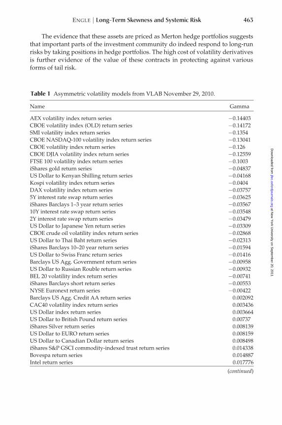
To examine this empirical measure, I look at estimates for almost 150assets which are followed every day in VLAB. This can easily be seen atwww.vlab.stern.nyu.edu. The assets include equity indices, international equityindices, individual names, sector indices, corporate bond prices, treasuries, com-modities, and volatilities, as well as currencies. The names of the series are givenin Table 1. These are sorted by the estimated value of Gamma, the asymmetricvolatility coefficient in the TARCH model. When this coefficient is negative, thenpositive returns predict higher volatility and when it is positive, negative returnspredict higher volatility.

From the argument given above, hedge portfolios should have negativegamma. From the list, it is clear that many of the assets naturally thought to behedge assets do indeed have negative gamma. This is true of eleven out of thir-teen volatility series. These series are constructed like the Market Volatility Index(VIX) but on a variety of assets including international equities and commodities.In each case, these assets will be expected to increase dramatically in value in an-other financial crisis. The next highest asset on the list is GOLD. It has a negativegamma.

US Treasuries appear to be a hedge, whether at the short or long end of thematurity. The swap rate variables are approximately converted to returns by usingthe negative of the log change in yield. In this way, these look very similar to thebond indices published by Barclays at the short, intermediate or long end of theterm structure.

Many exchange rates have negative gamma. As these are measured as dollarsper foreign currency, these should increase in a crisis if the foreign currency isexpected to weaken in a future crisis. We see that relative to the Kenyan, Japanese,Thai, Russian, and Swiss currencies, the volatility is asymmetric. Relative to manyothers, the exchange rate has the conventional positive sign. For most of theseother exchange rates, the coefficient is close to zero.

The large positive coefficients are typically broad-based equity indices, bothUS and global indices. This is consistent with the economic observation that in-dices that approximate the global wealth portfolio must have a positive gamma sothat returns and volatilities are negatively correlated.

at New

York U

niversity on Septem


Dow

nloaded from



The evidence that these assets are priced as Merton hedge portfolios suggeststhat important parts of the investment community do indeed respond to long-runrisks by taking positions in hedge portfolios. The high cost of volatility derivativesis further evidence of the value of these contracts in protecting against variousforms of tail risk.

Table 1 Asymmetric volatility models from VLAB November 29, 2010.

Name Gamma

AEX volatility index return series −0.14403CBOE volatility index (OLD) return series −0.14172SMI volatility index return series −0.1354CBOE NASDAQ-100 volatility index return series −0.13041CBOE volatility index return series −0.126CBOE DJIA volatility index return series −0.12559FTSE 100 volatility index return series −0.1003iShares gold return series −0.04837US Dollar to Kenyan Shilling return series −0.04168Kospi volatility index return series −0.0404DAX volatility index return series −0.037575Y interest rate swap return series −0.03625iShares Barclays 1–3 year return series −0.0356710Y interest rate swap return series −0.035482Y interest rate swap return series −0.03479US Dollar to Japanese Yen return series −0.03309CBOE crude oil volatility index return series −0.02868US Dollar to Thai Baht return series −0.02313iShares Barclays 10–20 year return series −0.01594US Dollar to Swiss Franc return series −0.01416Barclays US Agg. Government return series −0.00958US Dollar to Russian Rouble return series −0.00932BEL 20 volatility index return series −0.00741iShares Barclays short return series −0.00553NYSE Euronext return series −0.00422Barclays US Agg. Credit AA return series 0.002092CAC40 volatility index return series 0.003436US Dollar index return series 0.003664US Dollar to British Pound return series 0.00737iShares Silver return series 0.008139US Dollar to EURO return series 0.008159US Dollar to Canadian Dollar return series 0.008498iShares S&P GSCI commodity-indexed trust return series 0.014338Bovespa return series 0.014887Intel return series 0.017776

(continued)

at New

York U

niversity on Septem


Dow

nloaded from



Table 1 (continued)

Name Gamma

US Dollar to Australian Dollar return series 0.020536Hewlett-Packard return series 0.021733Barclays US Agg. credit BAA return series 0.02187US Dollar to Singapore dollar return series 0.02245MSCI Canada return series 0.023255Alcoa return series 0.028223Wal Mart stores return series 0.028549Caterpillar return series 0.031276AT&T return series 0.033125Du Pont return series 0.033618Charles Schwab return series 0.034797McDonalds return series 0.03503US Dollar to South Korean Won return series 0.036069Blackrock return series 0.037161CBOE Gold volatility index return series 0.039308Bank Of America return series 0.040501ML HY Cash Pay C All return series 0.042471General Motors return series 0.042776Boeing return series 0.043467CME Group return series 0.047192Franklin Resources return series 0.04838Walt Disney return series 0.048408General Electric return series 0.048818MBIA return series 0.048849Citigroup return series 0.049284Procter & Gamble return series 0.049897iShares Cohen & Steers Realty Majors return series 0.050613US Bancorp return series 0.052038Exxon Mobil return series 0.052686iShares Barclays MBS return series 0.052709MSCI FTSE/Xinhua China 25 return series 0.054102Coca Cola return series 0.055971Goldman Sachs return series 0.060912MSCI Taiwan return series 0.062269American Express return series 0.063519Materials SPDR return series 0.064714Korea composite stock index return series 0.064814Wells Fargo return series 0.064971Merck & Co. return series 0.065279iShares Dow Jones U.S. Real Estate return series 0.065537MSCI Japan return series 0.065731SPDR S&P Metals & Mining return series 0.066303Budapest Stock Exchange Index return series 0.066486

(continued)

at New

York U

niversity on Septem


Dow

nloaded from



Table 1 (continued)

Name Gamma

MSCI Italy return series 0.067246MasterCard return series 0.067339Energy SPDR return series 0.06862JP Morgan Chase return series 0.068975Johnson & Johnson return series 0.070134Home Depot return series 0.070361MSCI UK return series 0.073132iShares iBoxx $ High Yield Corporate return series 0.07341Fannie Mae return series 0.073971E-Trade return series 0.074877Technology SPDR return series 0.076638Utilities SPDR return series 0.077278MSCI Sweden return series 0.078147IBM return series 0.078657NASDAQ Composite return series 0.079284iShares S&P Global Energy return series 0.080881American Internation Group return series 0.081977Hang Seng return series 0.082658MSCI Spain return series 0.083193Consumer Staples SPDR return series 0.083752Russell 2000 return series 0.085299MSCI Germany return series 0.08642CIT Group return series 0.086607Consumer Discretionary SPDR return series 0.089509MSCI Australia return series 0.090098MSCI Switzerland return series 0.090125US Dollar to Indian Rupee return series 0.090441US Dollar to Indian Rupee return series 0.090441MSCI Netherlands return series 0.091247Morgan Stanley return series 0.091704MSCI France return series 0.091707MSCI Emerging Markets return series 0.094782FTSE 100 return series 0.097009MSCI Belgium return series 0.098846MSCI Hong Kong return series 0.099802CAC 40 return series 0.103081MSCI Brazil return series 0.103465MSCI World return series 0.103797Industrials SPDR return series 0.104001Prudential Financial return series 0.104334Financials SPDR return series 0.104509Dow Jones Industrials return series 0.105162SPDR S&P Oil & Gas Exp. & Prod. return series 0.105526

(continued)

at New

York U

niversity on Septem


Dow

nloaded from



Table 1 (continued)

Name Gamma

Wilshire Small Cap 250 return series 0.10599DAX 30 return series 0.106108iShares iBoxx $ Investment Grade Corporate return series 0.106886MSCI Singapore return series 0.107279MSCI EAFE return series 0.108903S&P 500 Composite return series 0.110646iShares S&P New York AMT-Free Municipal return series 0.111022MetLife return series 0.113888MSCI BRIC return series 0.113948Healthcare SPDR return series 0.115262United Technologies return series 0.11589MSCI FTSE China (HK Listed) return series 0.12127MSCI Mexico return series 0.140785ML HY Cash Pay B All return series 0.147277MIB 30 return series 0.191248

9 Conclusions

This paper introduces the idea that short- and long-run risk can be separatelymeasured and used to achieve investment goals. Failure to pay attention to long-term risk is a potential explanation for the financial crisis of 2007–2009 where lowshort term risk allowed financial institutions to load themselves with leverage andilliquid assets such as subprime Collateralized Debt Obligation (CDOs). Recogniz-ing that time-varying volatility models are able to measure how fast risk is likelyto evolve, the term structure of risk can be estimated by simulation. VaR, ES, andtail parameters can all be estimated. Because long-term skewness is more negativethan short-term skewness for typical volatility models, this becomes a key featureof long-term risk since negative skewness makes a major decline in asset valuesmore likely. In a Merton style model of defaults, it is shown that the negative long-term skewness can give rise to massive defaults and high correlations of defaultsreinforcing the possibility of another episode of systemic risk.

Although long-term negative skewness is a property of asymmetric volatilitymodels, there is no test for the strength of this effect. In this paper, such a test is de-veloped as a simulated method of moments test. From the asymptotic distributionand a Monte Carlo estimate of the distribution, it is found that all the asymmetricmodels are consistent with the long-term skewness in the data. It does not seemthat this will distinguish between models.

The economic underpinning of the asymmetric volatility model is developedfollowing French Schwert and Stambaugh and simple asset pricing theory. Themodel has implications for the proportion of return volatility that is due to changesin risk and the proportion due to changes in other factors such as cash flow. Affine

at New

York U

niversity on Septem


Dow

nloaded from



style models in discrete time provide a useful parameterization although this isnot necessarily the only way to express this relation.

Finally, economic agents that seek to hedge their long-term risk will naturallylook for Merton hedges that will outperform in bad states of nature. From standardasset pricing theory, it is possible to develop testable implications about the volatil-ity of such hedge portfolios. Remarkably, hedge portfolios should have asymmet-ric volatility of the opposite sign from ordinary assets. From examining close to 150volatility models in VLAB, it is discovered that the only ones with reverse asym-metric volatility are volatility derivatives themselves, treasury securities both longand short maturities, some exchange rates particularly relative to weak countriesand gold. These are all assets likely to be priced as hedge portfolios. There arecaveats in this procedure that argue for more research to investigate the power ofthis observation.

REFERENCES

Acharya, V., T. Cooley, M. Richardson, and I. Walter. 2010. Regulating Wall Street:The Dodd-Frank Act and the New Architecture of Global Finance. New York: WileyPublishing.

Acharya, V., and M. Richardson. 2009. Restoring Financial Stability: How to Repair aFailed System. New York: Wiley Publishing.

Bali, T., and R. Engle. 2010. The Intertemporal Capital Asset Pricing Model withDynamic Conditional Correlations. Journal of Monetary Economics 57: 377–390.

Barone-Adesi, G., R. Engle, and L. Mancini. 2008. A GARCH Option Pricing Modelwith Filtered Historical Simulation. Review of Financial Studies 21: 1223–1258.

Bekaert, G., and G. Wu. 2000. Asymmetric Volatility and Risk in Equity Markets.Review of Financial Studies 13: 1–42.

Berd, A., R. Engle, and A. Voronov. 2007. The Underlying Dynamics of CreditCorrelations. Journal of Credit Risk 3: 27–62.

Berndt, E., B. Hall, R. Hall, and J. Hausman. 1974. Estimation and Inference inNonlinear Structural Models. Annals of Social Measurement 3: 653–665.

Black, F. 1976. “Studies in Stock Price Volatility Changes.” Proceedings of the 1976Meeting of the American Statistical Association, Business and Economics Statistics Sec-tion. pp. 177–181.

Bollerslev, T. 2008. “Glossary to ARCH (GARCH).” CREATES Research Papers.2008–49. School of Economics and Management. University of Aarhus.

Brownlees, C., R. Engle, and B. Kelly. 2009. Evaluating Volatility Forecasts overMultiple Horizons. Working Paper, New York University.

Brunnermeier, M., A. Crockett, C. Goodhart, A. Persaud, and H. Shin. 2009. “TheFundamental Principles of Financial Regulation.” Geneva Reports on WorldEconomy 11. International Center for Monetary and Banking Studies.

Campbell, J., and L. Hentschel. 1992. No News is Good News: An AsymmetricModel of Changing Volatility in Stock Returns. Journal of Financial Economics 31:281–318.

at New

York U

niversity on Septem


Dow

nloaded from



Campbell, J., and R. Shiller. 1988. The Dividend Price Ratio and Expectations ofFuture Dividends and Discount Factors. Review of Financial Studies 1: 195–228.

Choi, J., and M. Richardson. 2008. “The Volatility of a Firm’s Assets.” AFA 2010Atlanta Meetings Paper.

Chou, R, R. Engle, and A. Kane. 1992. Measuring Risk Aversion from ExcessReturns on a Stock Index. Journal of Econometrics 52: 201–224.

Christie, A. 1982. The Stochastic Behavior of Common Stock Variances: Value,Leverage and Interest Rate Effects. Journal of Financial Economics 10: 407–432.

Davidson, R., and J. G. MacKinnon. 1993. Estimation and Inference in Econometrics.New York: Oxford University Press. 874 pages.

Engle, R. 1984. Wald, Likelihood Ratio and Lagrange Multiplier Tests in Economet-rics. Handbook of Econometrics 2: 776–826.

Engle, R. 2002. New Frontiers in ARCH Models. Journal of Applied Econometrics 17:425–446.

Engle, R. 2004. Risk and Volatility: Econometric Models and Financial Practice.Nobel Lecture. American Economic Review 94: 405–420.

Engle, R. 2009a. “Anticipating Correlations: A New Paradigm for Risk Management.”Princeton, New Jersey: Princeton University Press.

Engle, R. 2009b. The Risk that Risk Will Change. Journal of Investment Management7: 24–28.

Engle, R. 2009c. High Dimension Dynamic Correlations. The Methodology and Practiceof Econometrics: A Festschrift in David F. Hendry. Oxford: Oxford University Press.

Engle, R., and I. Ishida. 2002. “Forecasting Variance of Variance: The Square-root,the Affine and the CEV GARCH Models.” New York University Working Paper.

Engle, R., D. Lilien, and R. Robins. 1987. Estimation of Time Varying Risk Premiain the Term Structure: the ARCH-M Model. Econometrica 55: 391–407.

French, K., G. Schwert, and R. Stambaugh. 1987. Expected Stock Returns andVolatility. Journal of Financial Economics 19: 3–30.

Godfrey, L. G., and M. R. Wickens. 1981. Testing Linear and Log-Linear Regres-sions for Functional Form. Review of Economic Studies 48: 487–496.

Guidolin, M. and A. Timmermann. 2006. Term Structure of Risk under AlternativeEconometric Specifications. Journal of Econometrics 131: 285–308.

Kelly, B. 2009. “Risk Premia and the Conditional Tails of Stock Returns.” New YorkUniversity Working Paper.

McNeil, A., P. Embrechts, and R. Frey. 2005. Quantitative Risk Management.Princeton, New Jersey: Princeton University Press, Princeton Series in Finance.

Medahi, N., and E. Renault. 2004. Temporal Aggregation of Volatility Models.Journal of Econometrics 119: 355–379.

Merton, R. 1973. An Intertemporal Capital Asset Pricing Model. Econometrica 41:867–887.

Resnick S. I., and C. Starica. 1995. Consistency of Hill’s Estimator for DependentData. Journal of Applied Probability 32: 139–167.

Smith, D., and R. Whitelaw. 2009. “Time-Varying Risk Aversion and the Risk-Return Relation.” New York University Working Paper.

at New

York U

niversity on Septem


Dow

nloaded from


long-term skewness and systemic risk - · pdf filelong-term skewness and systemic risk ......

Documents