long-term simulation of objects in high-earth...

ESA/ESOC Contract to ISTI/CNR

“Analysis of Mitigation Measures based on the Semi-Deterministic Model” Contract No. 18423/04/D/HK

Long-Term Simulation of Objects in High-Earth Orbits

Study Note of Work Package No. 2 Part I

Version 1.0

Prepared by

Luciano Anselmo and Carmen Pardini

13 December 2006

Space Flight Dynamics Laboratory

Istituto di Scienza e Tecnologie dell’Informazione “A. Faedo” CNR – Area della Ricerca di Pisa

Via G. Moruzzi 1, 56124 Pisa, Italy

http://www.cnr.it/ITA/testo.htm

ESA/ESOC Contract No. 18423/04/D/HK WP-2: Long-Term Simulation of Objects in High-Earth Orbits Final Study Note – Part I – Version 1.0 – 13 December 2006

TABLE OF CONTENTS

ABSTRACT _______________________________________________________________ 2

1. INTRODUCTION ________________________________________________________ 3 1.1 Task Description ____________________________________________________________ 3 1.2 Orbit Propagator ___________________________________________________________ 3

2. GEO DISPOSAL ORBITS__________________________________________________ 5 2.1 The IADC Formula__________________________________________________________ 5 2.2 Long-Term Evolution of Objects in GEO Disposal Orbits __________________________ 6

2.2.1 Evolution as a Function of Ω + ω____________________________________________________ 7 2.2.2 Evolution as a Function of the Perigee Orientation w.r.t. the Sun ___________________________ 9 2.2.3 Evolution as a Function of Eccentricity ______________________________________________ 11 2.2.4 Evolution as a Function of Inclination _______________________________________________ 15 2.2.5 Evolution as a Function of ΩM _____________________________________________________ 17

2.3 Summary _________________________________________________________________ 18

3. SYNCHRONOUS OBJECTS WITH HIGH A/M_______________________________ 20 3.1 The Discovery of Geosynchronous Debris ______________________________________ 20 3.2 Long-Term Evolution of GEO Objects with High A/M ___________________________ 20 3.3 Summary _________________________________________________________________ 24

4. LIFETIME OF MOLNIYA ORBITS ________________________________________ 25 4.1 Introduction_______________________________________________________________ 25 4.2 Long-Term Evolution of Molniya Orbits _______________________________________ 27 4.3 Lifetimes of Molniya and Oko Orbits __________________________________________ 39 4.4 Disposal of Satellites in Molniya Orbits ________________________________________ 40

GLOSSARY ______________________________________________________________ 41

REFERENCES ___________________________________________________________ 42

1


ABSTRACT This report (Part I of the Study Note of Work Package 2) presents the results obtained by applying the most accurate and complete long-term orbit propagator used in SDM 4.0 to study specific problems involving the MEO and GEO orbital regimes. In particular, the following topics were investigated:

1. The long-term evolution of GEO disposal orbits and the role in it of the initial eccentricity vector;

2. The identification of initial orbit elements and area-to-mass ratios leading to synchronous high eccentricity orbits like those recently discovered by the ESA 1 m telescope in Tenerife;

3. The orbital lifetime of objects in Molniya-like orbits as a function of initial conditions and operational practice.

The long-term evolution of objects placed in the graveyard orbits used or proposed for the navigation satellites in MEO, in particular Galileo, is addressed in a companion report (Part II of the Study Note of Work Package 2).

2


1. INTRODUCTION 1.1 Task Description The goal of this work package was to address the long-term (200 years) orbital evolution of objects in MEO (e.g. Molniya, GPS, Galileo, etc…) and GEO. In particular, the following investigations were foreseen [1]: • Study of the long-term evolution of objects disposed of in GEO graveyard orbits as a

function of the initial orbital elements, in particular the eccentricity vector, in order to identify the possible return of such objects in the GEO protected region, due to the effects of the orbital perturbations;

• Identification of initial orbit elements and area-to-mass ratios leading to synchronous high eccentricity orbits like those recently discovered by the ESA 1 m telescope in Tenerife;

• Analysis of the orbital lifetime of objects in Molniya orbits as a function of initial conditions;

• Study of the long-term evolution of objects placed in the graveyard orbits used or proposed for the navigation satellites in MEO, in particular Galileo, and investigation of the possibility to exploit the orbital perturbations to determine a natural decay within a few decades.

These study objectives were fulfilled using only a subset of the new SDM functionalities, namely the orbit propagator for the MEO and GEO orbital regimes. During the first phase of the activity, extensive analyses were carried out for testing purposes, comparing different approaches and available models, with the aim of identifying and implementing appropriate trajectory propagators and model options to study the long-term orbital evolution of objects in MEO and GEO. The results obtained were described in the Progress Report No. 1 [2]. 1.2 Orbit Propagator The studies listed in the previous section and presented in this study note were carried out using a stand-alone version of the FOP propagator implemented in SDM [2]. It uses the variation of parameters method in the formulation of the equations of motion. The perturbations taken into account are: the Earth’s geopotential, the third body attraction of the Moon and the Sun, the air drag (when applicable) and the solar radiation pressure, including the eclipses. To expedite the computations, the terms including the mean anomaly (fast variable) are removed in the Earth’s and third-body potentials before numerical integration (singly averaged method). On the other hand, when resonances occur between the orbital

3


period and the Earth rotation, the terms containing the mean anomaly in the tesseral harmonics of the geopotential are retained, giving rise to resonant effects. To average the potential due to solar radiation pressure and air drag, a standard 8th order Gaussian quadrature method is used. The resulting averaged equations are integrated numerically using a multi-step, variable step-size and variable order method. The computation time is maintained under control, without compromising the accuracy, due to the elimination of the fast variable and the possibility of using large step sizes (days). Being the present study focused on GEO and MEO orbital regimes, the drag perturbation was included only to model high eccentricity orbits (e.g. Molniya orbits). In such cases, taking into account the purposes of the analysis and the very long time intervals considered (up to 200 years), a simple exponential atmospheric density model, with the parameters shown in Table 1.1, was adopted.

Table 1.1

Parameters of the Exponential Atmospheric Density Model and Drag Perturbation

Termospheric Density Model Jacchia-71 Exospheric Temperature 1000 K

Reference Altitude for Air Density 400 km Scale Height of Air Density 55.92 km

Air Density at Reference Altitude 3.11 x 10-3 kg/km3 Maximum Altitude to Include Drag 1000 km

Drag Coefficient 2.2

4


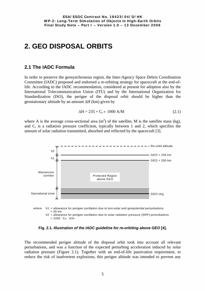
2. GEO DISPOSAL ORBITS 2.1 The IADC Formula In order to preserve the geosynchronous region, the Inter-Agency Space Debris Coordination Committee (IADC) proposed and endorsed a re-orbiting strategy for spacecraft at the end-of-life. According to the IADC recommendation, considered at present for adoption also by the International Telecommunication Union (ITU) and by the International Organization for Standardization (ISO), the perigee of the disposal orbit should be higher than the geostationary altitude by an amount ∆H (km) given by

∆H = 235 + Cr × 1000 A/M (2.1) where A is the average cross-sectional area (m2) of the satellite, M is the satellite mass (kg), and Cr is a radiation pressure coefficient, typically between 1 and 2, which specifies the amount of solar radiation transmitted, absorbed and reflected by the spacecraft [3].

where h1 = allowance for perigee oscillation due to luni-solar and geopotential perturbations= 35 km

h2 = allowance for perigee oscillation due to solar radiation pressure (SRP) perturbations= 1000 ⋅ CR ⋅ A/m

Protected Regionabove GEO

Manoeuvrecorridor

Operational zone

h1

h2

GEO ring

GEO + 200 km

GEO + 235 km

Re-orbit altitude

Fig. 2.1. Illustration of the IADC guideline for re-orbiting above GEO [4]. The recommended perigee altitude of the disposal orbit took into account all relevant perturbations, and was a function of the expected perturbing acceleration induced by solar radiation pressure (Figure 2.1). Together with an end-of-life passivation requirement, to reduce the risk of inadvertent explosions, this perigee altitude was intended to prevent any

5


further interference with a properly defined geostationary protected region, consisting of a toroid centered on the geostationary orbit, extending 200 km above and below this altitude and ± 15° in declination. While normal operations are usually conducted in the so-called geostationary ring, within 75 km of the geostationary altitude and ± 0.1° in declination, the protected region was extended in altitude (± 200 km), to create a maneuver corridor for spacecraft relocation (plus a margin), and in declination (± 15°), to take into account the natural orbit evolution of geosynchronous satellites without inclination control. In order to avoid any further interference with the geostationary protected region, Eq. (2.1) – specifically the term dealing with solar radiation pressure – was developed with the underlying hypothesis of a nearly circular disposal orbit. However, this legacy was lost in the end-of-life re-orbiting requirement written in the IADC Space Debris Mitigation Guidelines [3], even because several analysts had become convinced that disposal eccentricities different from zero might in the long-term have ensured lower spatial densities and collision probabilities in the super-synchronous graveyard region. However, subsequent analyses of the stability of super-synchronous graveyard orbits, for example by Martin et al. [5], but especially by Lewis et al. [6], confirmed the validity of the hypothesis underlying Eq. (2.1). In other words, the success of the re-orbiting defined by the IADC formula in avoiding any further crossing of the geostationary protected region depended upon attaining a disposal eccentricity that was as small as possible (≤ 0.005). Other studies, on the other hand, pointed out the potential of eccentricity vector control. For instance, by pointing the disposal orbit perigee towards the Sun and targeting the “natural” eccentricity induced by solar radiation pressure, it would be possible to preserve the protected region with a slightly smaller altitude increase than that found with the IADC formula [7]. It was also found that even eccentricities as large as 0.05 did not cause any further interference with the geostationary protected region, provided a proper orientation of the eccentricity vector was achieved after re-orbiting [8]. In order to clarify the matter, an extensive analysis was carried out at ISTI/CNR, which investigated in depth the influence of the eccentricity vector magnitude and direction, in addition to other relevant initial conditions and parameters. This activity was an extension of an international study promoted by IADC, to explore the evolution and stability of super-synchronous disposal orbits [9][10]. Afterwards, such an analysis was further refined and extended, and the results obtained are presented in the following section. 2.2 Long-Term Evolution of Objects in GEO Disposal Orbits The simulations, spanning 200 years, focused on the re-orbiting of spacecraft with A/M = 0.02 m2/kg and Cr = 1.2 (representative average values for geostationary satellites). They considered a disposal perigee altitude according to the IADC formula, eccentricities up to 0.5, inclinations up to 15°, varying perigee angles (α) with respect to the right ascension of the Sun, varying values of the right ascension of the ascending node plus the argument of perigee (Ω + ω) and different values of the initial right ascension of the ascending node of the Moon

6


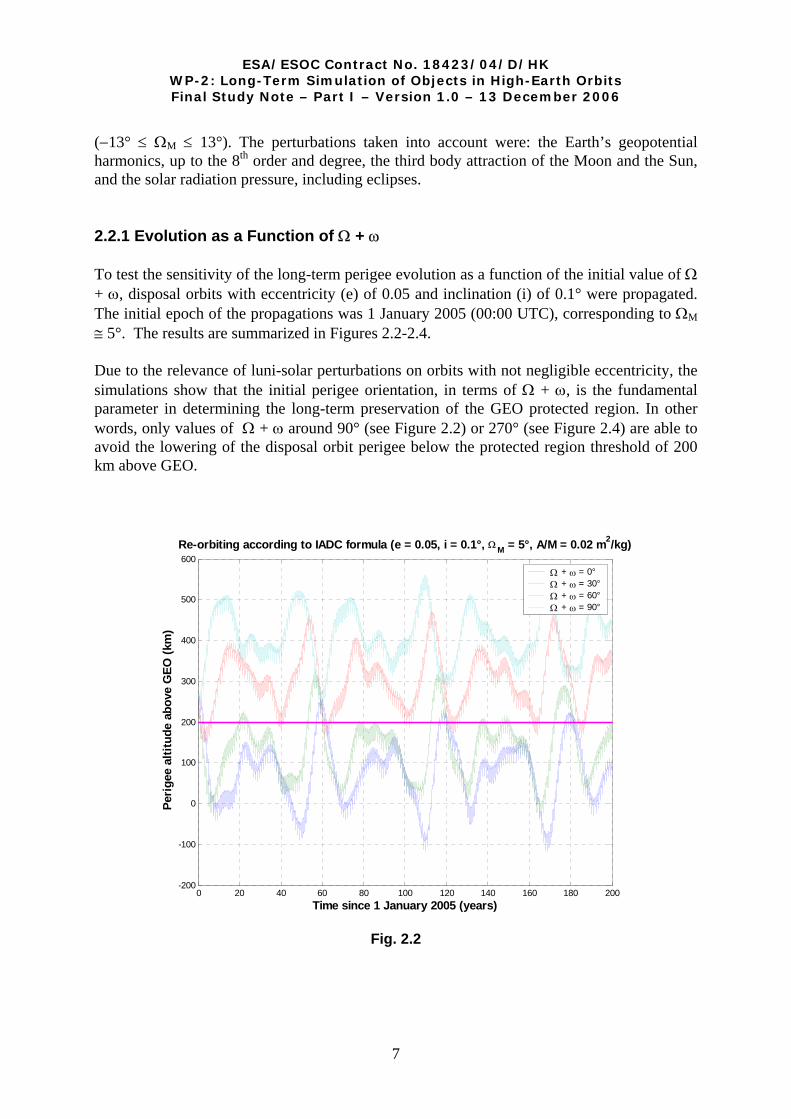
(−13° ≤ ΩM ≤ 13°). The perturbations taken into account were: the Earth’s geopotential harmonics, up to the 8th order and degree, the third body attraction of the Moon and the Sun, and the solar radiation pressure, including eclipses. 2.2.1 Evolution as a Function of Ω + ω To test the sensitivity of the long-term perigee evolution as a function of the initial value of Ω + ω, disposal orbits with eccentricity (e) of 0.05 and inclination (i) of 0.1° were propagated. The initial epoch of the propagations was 1 January 2005 (00:00 UTC), corresponding to ΩM ≅ 5°. The results are summarized in Figures 2.2-2.4. Due to the relevance of luni-solar perturbations on orbits with not negligible eccentricity, the simulations show that the initial perigee orientation, in terms of Ω + ω, is the fundamental parameter in determining the long-term preservation of the GEO protected region. In other words, only values of Ω + ω around 90° (see Figure 2.2) or 270° (see Figure 2.4) are able to avoid the lowering of the disposal orbit perigee below the protected region threshold of 200 km above GEO.

0 20 40 60 80 100 120 140 160 180 200-200

-100

0

100

200

300

400

500

600Re-orbiting according to IADC formula (e = 0.05, i = 0.1°, ΩM = 5°, A/M = 0.02 m2/kg)

Time since 1 January 2005 (years)

Peri

gee

altit

ude

abov

e G

EO (k

m)

Ω + ω = 0°Ω + ω = 30°Ω + ω = 60°Ω + ω = 90°

Fig. 2.2

7


0 20 40 60 80 100 120 140 160 180 200-200

-100

0

100

200

300

400



Perig

ee a

ltitu

de a

bove

GEO

(km

)Ω + ω = 120°Ω + ω = 150°Ω + ω = 180°Ω + ω = 210°

Fig. 2.3

0 20 40 60 80 100 120 140 160 180 200-100

0

100

200

300

400

500



Perig

ee a

ltitu

de a

bove

GEO

(km

)

Ω + ω = 240°Ω + ω = 270°Ω + ω = 300°Ω + ω = 330°

Fig. 2.4

8


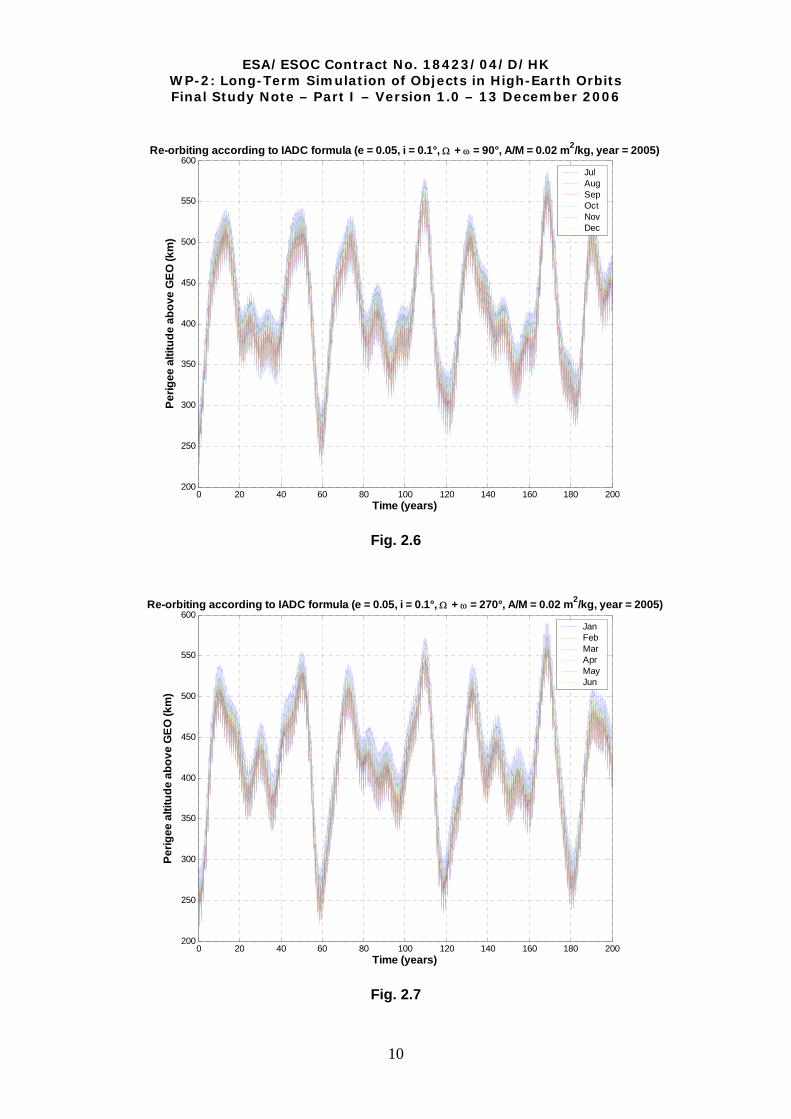
2.2.2 Evolution as a Function of the Perigee Orientation w.r.t. the Sun The long-term perigee evolution is also affected by solar radiation pressure and, therefore, by the initial orientation of the perigee vector with respect to the Sun. However, for standard satellites, characterized by A/M << 1 m2/kg, this effect becomes dominant only for e < 0.005. At larger eccentricities, as exemplified by the simulations discussed in the previous section, the perigee evolution is mainly driven by luni-solar perturbations and the critical parameter is the initial value of Ω + ω. In order to quantify the relative importance of the initial orientation of the perigee vector with respect to the Sun, disposal orbits with eccentricity (e) of 0.05, inclination (i) of 0.1° and a fixed value of Ω + ω (either 90° or 270°) were propagated at the beginning of each month of 2005 to simulate varying perigee angles (α) with respect to the right ascension of the Sun. Concerning the right ascension of the ascending node of the Moon, the initial epochs of the propagations corresponded to 3° ≤ ΩM ≤ 5°. The results for Ω + ω = 90° are summarized in Figures 2.5 and 2.6. As anticipated, the details of the perigee altitude evolution are a function of the initial perigee orientation with respect to the Sun, but the main pattern of evolution is driven by Ω + ω, that is by luni-solar perturbations. An approximately Sun-pointing perigee – occurring in the 1 June (α ≅ 21°) and 1 July (α ≅ −10°) propagations, in this example – may increase the minimum perigee altitude

0 20 40 60 80 100 120 140 160 180 200200

250

300

350

400

450

500

550

600Re-orbiting according to IADC formula (e = 0.05, i = 0.1°, Ω + ω = 90°, A/M = 0.02 m2/kg, year = 2005)

Time (years)

Perig

ee a

ltitu

de a

bove

GEO

(km

)

JanFebMarAprMayJun

Fig. 2.5

9


0 20 40 60 80 100 120 140 160 180 200200

250

300

350

400

450

500

550


Time (years)

Perig

ee a

ltitu

de a

bove

GEO

(km

)JulAugSepOctNovDec

Fig. 2.6

0 20 40 60 80 100 120 140 160 180 200200

250

300

350

400

450

500

550


Time (years)

Perig

ee a

ltitu

de a

bove

GEO

(km

)

JanFebMarAprMayJun

Fig. 2.7

10


0 20 40 60 80 100 120 140 160 180 200200

250

300

350

400

450

500

550


Time (years)

Perig

ee a

ltitu

de a

bove

GEO

(km

)JulAugSepOctNovDec

Fig. 2.8

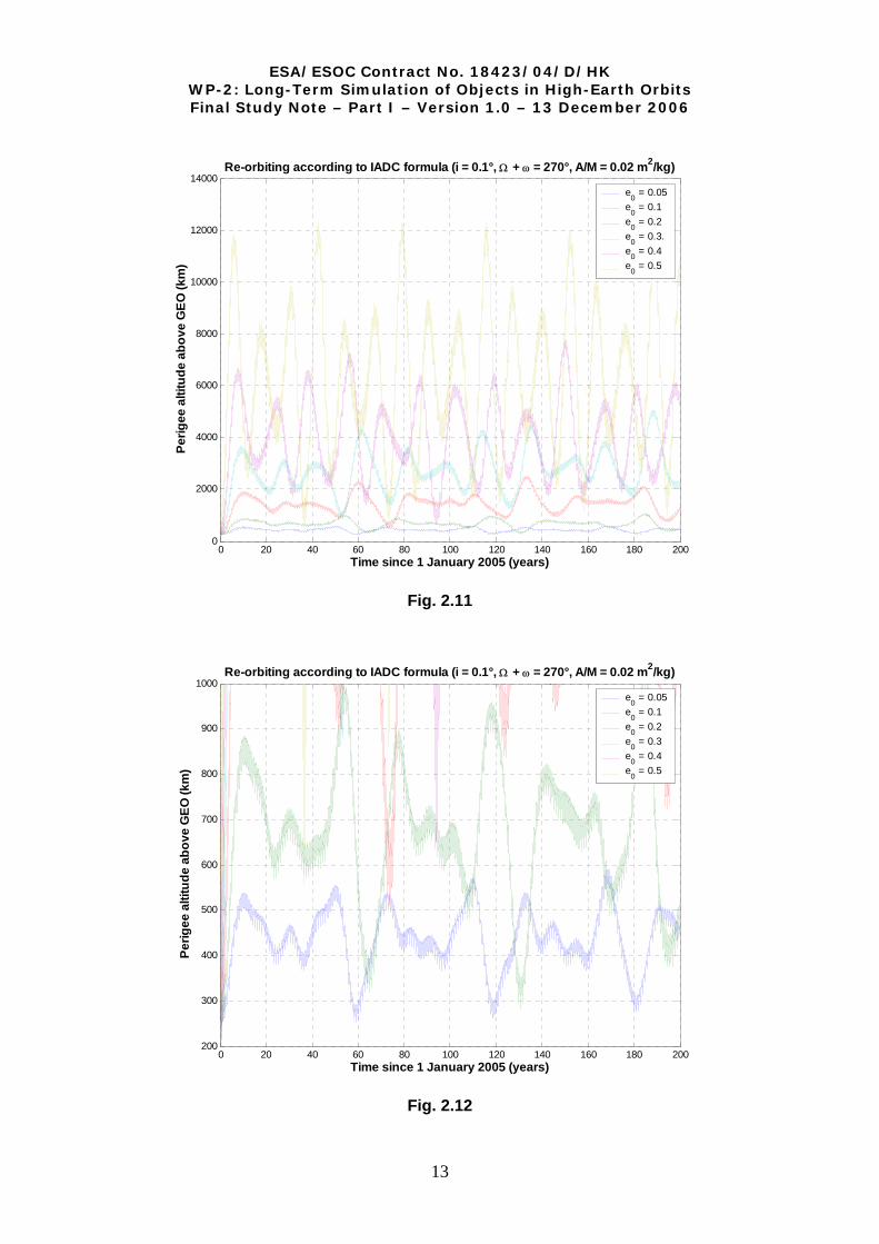
by ∼ 30 km with respect to the worst cases, observed when α is either close to 100° (1 March) or −100° (1 October). However, the appropriate choice of the initial value of Ω + ω would guarantee, in any case, the preservation of the protected region, irrespective of the perigee vector orientation with respect to the Sun. The results for Ω + ω = 270° display the same behavior and are summarized in Figures 2.7 and 2.8. Again, an approximately Sun-pointing perigee – occurring in the 1 December (α ≅ 23°) and 1 January (α ≅ −12°) propagations, in this example – may increase the minimum perigee altitude by ∼ 30 km with respect to the worst cases, observed when α is either close to 100° (1 September) or −100° (1 April). But, in any case, the appropriate choice of the initial value of Ω + ω would guarantee the long-term preservation of the protected region. 2.2.3 Evolution as a Function of Eccentricity Even though, due to propellant budget considerations, GEO disposal orbits will be constrained to low eccentricity values (typically < 0.01), the stability of high eccentricity disposal orbits, in agreement with the IADC formula, was investigated as well, up to e = 0.5. The sensitivity analysis was carried out assuming an initial inclination of 0.1° and a fixed value of Ω + ω (either 90° or 270°). The initial epoch of the propagations was 1 January 2005 (00:00 UTC), corresponding to ΩM ≅ 5°. The results obtained are summarized in Figures 2.9-2.12.

11


0 20 40 60 80 100 120 140 160 180 2000

2000

4000

6000

8000

10000

12000

14000Re-orbiting according to IADC formula (i = 0.1°, Ω + ω = 90°, A/M = 0.02 m2/kg)


Peri

gee

altit

ude

abov

e G

EO (k

m)

e0 = 0.05e0 = 0.1e0 = 0.2e0 = 0.3e0 = 0.4e0 = 0.5

Fig. 2.9

0 20 40 60 80 100 120 140 160 180 200200

300

400

500

600

700

800

900



Perig

ee a

ltitu

de a

bove

GEO

(km

)

e0 = 0.05e0 = 0.1e0 = 0.2e0 = 0.3e0 = 0.4e0 = 0.5

Fig. 2.10

12


0 20 40 60 80 100 120 140 160 180 2000

2000

4000

6000

8000

10000

12000



Perig

ee a

ltitu

de a

bove

GEO

(km

)e0 = 0.05e0 = 0.1e0 = 0.2e0 = 0.3.e0 = 0.4e0 = 0.5

Fig. 2.11

0 20 40 60 80 100 120 140 160 180 200200

300

400

500

600

700

800

900



Perig

ee a

ltitu

de a

bove

GEO

(km

)

e0 = 0.05e0 = 0.1e0 = 0.2e0 = 0.3e0 = 0.4e0 = 0.5

Fig. 2.12

13


The outcome of the simulations is very clear: a proper choice of the initial value of Ω + ω can guarantee the long-term preservation of the GEO protected region even with disposal orbits, following the IADC formula, characterized by very high (and unrealistic) eccentricities (see, in particular, Figures 2.10 and 2.12). This is a quite surprising result. In addition, the minimum perigee altitude observed after disposal in the simulated time span increases at larger eccentricities, up to e ∼ 0.3. But, in any case, the object density at perigee is diluted over a greater volume of space and the average perigee altitude increases with growing eccentricity in the entire interval of considered values, up to e = 0.5 (see Figures 2.9 and 2.11). For e > 0.5, the apogee altitude becomes so high (> 120,000 km) that a perturbative approach cannot be longer used to model accurately the attraction of the Moon. This is the reason why the analysis presented in this section was limited to e = 0.5. For small eccentricities, typically ≤ 0.005, solar radiation pressure becomes more important than luni-solar perturbations and the long-term evolution of the perigee altitude is mainly driven by the parameter α, instead of Ω + ω. Figures 2.13 and 2.14 show the results obtained with a disposal orbit eccentricity of 0.005. Even though, in this case, any combination of α and Ω + ω is able to guarantee the long-term preservation of the GEO protected region, provided that the IADC re-orbiting formula is adopted, an approximately Sun-pointing perigee vector (α = 0°) is clearly the best solution in order to maximize the long-term perigee altitude. By choosing a Sun-pointing eccentricity vector, it would also be possible to preserve

2010 2020 2030 2040 2050 2060 2070 2080 2090 2100200

220

240

260

280

300

320

340Re-orbiting according to IADC formula (e = 0.005, i = 0.1°, A/M = 0.02 m2/kg)

Year

Perig

ee a

ltitu

de a

bove

GEO

(km

)

α = 0°, Ω + ω = 282°α = 45°, Ω + ω = 327°α = 90°, Ω + ω = 12°

Protected Region

Fig. 2.13

14


2010 2020 2030 2040 2050 2060 2070 2080 2090 2100

200

220

240

260

280

300

320

340Re-orbiting according to IADC formula (e = 0.005, i = 0.1°, A/M = 0.02 m2/kg)

Year

Perig

ee a

ltitu

de a

bove

GEO

(km

)α = 0°, Ω + ω = 282°α = 180°, Ω + ω = 102°

Upper Limit of GEO Protected Region

Fig. 2.14

the GEO protected region with a re-orbiting altitude smaller than that prescribed by the IADC formula, with a non-negligible propellant saving. 2.2.4 Evolution as a Function of Inclination The sensitivity of the long-term perigee evolution as a function of the initial value of the disposal orbit inclination was investigated as well. In fact, geosynchronous spacecraft for which north-south station keeping is no longer applied, in order to save propellant and extend their useful life, may be re-orbited, in theory, with 0° ≤ i ≤ 15°. Therefore, disposal orbits with e = 0.05 and a fixed value of Ω + ω (either 90° or 270°) were propagated with various values of the initial inclination (i0) in the interval of interest. The initial epoch of the propagations was 1 January 2005 (00:00 UTC), corresponding to ΩM ≅ 5°. The results are summarized in Figures 2.15 and 2.16. They show that, with a proper choice of the initial value of Ω + ω, in order to maintain under control the effects of luni-solar perturbations, the long-term return of the re-orbited satellites in the GEO protected region may also be avoided with substantial initial inclinations, up to ∼ 10°. The details depend, however, on the initial conditions and should be determined on a case-by-case basis.

15


0 20 40 60 80 100 120 140 160 180 2000

100

200

300

400

500

600

700Re-orbiting according to IADC formula (e = 0.05, Ω +ω = 90°, ΩM = 5°, A/M = 0.02 m2/kg)


Perig

ee a

ltitu

de a

bove

GEO

(km

)i0 = 0.1°i0 = 1°i0 = 5°i0 = 10°i0 = 15°

Fig. 2.15

0 20 40 60 80 100 120 140 160 180 200100

200

300

400

500

600

700Re-orbiting according to IADC formula (e = 0.05, Ω + ω = 270°, ΩM = 5°, A/M = 0.02 m2/kg)


Perig

ee a

ltitu

de a

bove

GEO

(km

)

i0 = 0.1°i0 = 1°i0 = 5°i0 = 10°i0 = 15°

Fig. 2.16

16


2.2.5 Evolution as a Function of ΩM The long-term evolution of the perigee altitude of the GEO disposal orbits is also affected by the initial right ascension of the Moon ascending node (ΩM), varying approximately between −13° and +13° with a period of 18.6 years, i.e. the period of regression of the longitude of the Moon ascending node with respect to the ecliptic plane. Due to the long period of the ΩM oscillation, its initial value cannot be chosen by the satellite operator, depending on the date in which the re-orbiting occurs. In order to evaluate its effects on the long-term evolution of the perigee altitude, disposal orbits with e = 0.05, i = 0.1° and a fixed value of Ω + ω (either 90° or 270°) were propagated with various values of the initial ΩM in the interval of interest. The results obtained are summarized in Figures 2.17 and 2.18. The initial right ascension of the Moon ascending node clearly affects the perigee evolution, but for the cases considered (e = 0.05 and A/M = 0.02 m2/kg) its impact (∼ 50 km between the “best” case, ΩM = 0°, and the “worst” cases, ΩM ≅ ± 13°) is comparable to that of the α parameter, i.e. the variation of solar radiation pressure effects due to the varying initial orientation of the perigee vector with respect to the Sun.

0 20 40 60 80 100 120 140 160 180 200200

250

300

350

400

450

500

550

600Re-orbiting according to IADC formula (e = 0.05, i = 0.1°, Ω + ω = 90°, A/M = 0.02 m2/kg)

Time (years)

Peri

gee

altit

ude

abov

e G

EO (k

m)

ΩM = +13°, α = -10°ΩM = +5°, α = 168°ΩM = 0°, α = 0°ΩM = -13°, α = -10°

Fig. 2.17

17


0 20 40 60 80 100 120 140 160 180 200200

250

300

350

400

450

500

550

600Re-orbiting according to IADC formula (e = 0.05, i = 0.1°, Ω + ω = 270°, A/M = 0.02 m2/kg)

Time (years)

Perig

ee a

ltitu

de a

bove

GEO

(km

)ΩM = +13°, α = 170°ΩM = +5°, α = -12°ΩM = 0°, α = 180°ΩM = -13°, α = 170°

Fig. 2.18

In any case, the proper choice of the initial value of Ω + ω is able to avoid the long-term return of the re-orbited satellites in the GEO protected region. On the other hand, by fixing at the re-orbiting epoch the value of Ω + ω to minimize the adverse impact of luni-solar perturbations, it is impossible, in practice, to choice either α or ΩM, keeping separated their effects. 2.3 Summary Concerning the end-of-life disposal of geosynchronous satellites according to the IADC recommendation and the long-term preservation of the GEO protected region, the main conclusions of the analysis presented in this chapter are the following: • The IADC re-orbiting formula can prevent the long-term crossing of the geostationary

protected region only by constraining the initial eccentricity vector; • An unconstrained perigee vector translates into a maximum acceptable eccentricity of ∼

0.005; • Eccentricities as large as 0.5 are acceptable with an appropriate perigee orientation driven

by luni-solar perturbations (Ω + ω ≅ 90° or 270°); • Initial inclinations as large as ∼ 10° are acceptable with Ω + ω ≅ 90° or 270°;

18


• The details of the evolution depend on initial state vector, right ascension of the Sun, right ascension of the Moon ascending node and CrA/M, and should be investigated on a case-by-case basis;

• Increasing the re-orbiting altitude is not a viable alternative to eccentricity vector control [2][9];

• For small eccentricities, the choice of a Sun-pointing perigee may result in a lower altitude increase, with respect to the IADC formula, which is able to preserve the geostationary protected region with a velocity variation, or propellant saving, of ∼ 15%;

• For eccentricities > 0.005, optimal solutions, in terms of maximum long-term separation from the geostationary protected region, can generally be obtained by combining the proper choice of Ω + ω (∼ 90° or ∼ 270°) with a Sun-pointing perigee and ΩM ∼ 0°. Unfortunately, for the assigned values of Ω + ω, a Sun-pointing perigee is possible only in certain periods of the year (around June, for Ω + ω ∼ 90°, and around December, for Ω + ω ∼ 270°), while the value of ΩM, varying with a period of 18.6 years, is basically a function of the year of disposal.

Therefore, the IADC formula can in fact guarantee its intended goal only by constraining the disposal orbit eccentricity. If the disposal perigee is left unconstrained, the graveyard orbit must be nearly circular, with an eccentricity typically smaller than 0.005. However, for small eccentricities, comparable to the natural values induced by solar radiation pressure, a Sun-pointing perigee may result in a slightly more efficient re-orbiting strategy, compared to Eq. (2.1), which is able to avoid any further interference with the geostationary protected region. On the other hand, for eccentricities larger than the natural value induced by solar radiation pressure, the eccentricity vector evolution is driven by luni-solar perturbations. In these cases, an unconstrained disposal eccentricity vector may produce large variations in the perigee altitude and the consequent violation of the protected region. However, due to the form of the second order luni-solar perturbation term [11], at Ω + ω ≅ 90° ± 15° or 270° ± 15° the perigee altitude evolution can guarantee the long-term preservation of the geostationary protected region, even with initial disposal eccentricities as large as 0.5. The details depend, of course, on the initial conditions, such as the eccentricity, the inclination, the season (i.e. the right ascension of the Sun), and the right ascension of the Moon ascending node. But the conclusion remains the same: even significant (and unrealistic – from a propellant budget point of view) re-orbiting eccentricities may be acceptable, in terms of preserving the geostationary protected region, provided that the disposal orbit perigee is oriented so as to minimize the altitude variations induced by the luni-solar perturbations.

19


3. SYNCHRONOUS OBJECTS WITH HIGH A/M 3.1 The Discovery of Geosynchronous Debris Optical observations have discovered a substantial amount of decimeter sized objects in orbits close to the geosynchronous altitude [12][13][14][15]. Most of these are probably the result of a still undetermined number of explosions occurred to spacecraft and upper stages. So far, however, only two fragmentations have been confirmed near the geostationary orbit [16] and the identification of further explosions at a so high altitude is complicated by the long time passed since the occurrence of the events and by the effects of the orbital perturbations on the resulting debris clouds [17][18]. Recent observations, carried out by the ESA’s 1 m telescope in Tenerife, have identified an additional population of faint uncatalogued objects, with mean motions of about 1 revolution per day and orbital eccentricities as high as 0.55 [19]. The discovery of such objects was quite surprising, but an obvious explanation for their origin was immediately proposed. In fact, direct solar radiation pressure may significantly affect the eccentricity with small effects on the total energy of the orbit and, therefore, on the semi-major axis or mean motion. However, this perturbation is adequately effective only on objects with sufficiently high area-to-mass ratios [20]. 3.2 Long-Term Evolution of GEO Objects with High A/M The dynamical evolution of objects released in geostationary orbit with area-to-mass ratios (A/M) between 1 and 50 m2/kg, Cr = 1.2 and negligible relative velocity has been analyzed in detail, both short and long-term, elsewhere [21][22], taking into account the Earth’s geopotential harmonics up to the 8th order and degree, luni-solar perturbations, direct solar radiation pressure with eclipses and, when applicable, air drag. As shown by the simulations carried out, a very rapid growth in eccentricity (Figure 3.1) is expected, strongly correlated with A/M: the greater the latter, the larger the effect. Objects above a certain A/M threshold (40-45 m2/kg, depending on the initial conditions) develop an eccentricity so large, and a perigee so low, that decay from orbit in less than six months is induced. The objects below this A/M threshold are not subject to this fate. In fact, after approximately six months their eccentricity inverts the trend, reaching a new minimum just about one year after release. This “short-term” annual oscillation may reach very significant amplitudes, depending on the value of the average area-to-mass ratio. As shown in Figure 3.1, debris with A/M ∼ 20 m2/kg would be characterized by annual oscillations of the eccentricity with amplitude of about 0.5. Objects of this kind are, therefore, obvious candidates to explain the recently discovered population of synchronous debris with high eccentricity.

20


0 10 20 30 40 500

0.1

0.2

0.3

0.4

0.5

0.6

0.7

0.8

0.9

Area-to-Mass Ratio (m2/kg)

Mea

n Ec

cent

rici

ty

1 month2 months3 months4 months6 months1 year

Fig. 3.1. Short-term eccentricity evolution of objects released in geostationary orbit as

a function of area-to-mass ratio and elapsed time. The details may vary slightly depending on the initial conditions.

Being the orbital decay – if any – typically induced by an eccentricity growth and a sudden decrease of the perigee height, the semi-major axis and the orbital period remain close to the geosynchronous ones until the actual reentry [2][21]. In other words, high A/M objects subjected to the evolution described in this section maintain a geosynchronous motion even when their eccentricity assumes extremely elevated values, again in agreement with the observational results. The inclination too is expected to grow very rapidly as a function of the area-to-mass ratio (Figure 3.2). In this case, however, a relatively small “short-term” fluctuation, with a period of almost one year, due to the prevalence of solar radiation pressure over luni-solar perturbations, is masked by a significantly larger long-term effect, due to the combined out-of-plane disturbance induced by solar radiation pressure, luni-solar third body attraction and even zonal harmonics of the geopotential (Figures 3.3 and 3.4).

21


0 10 20 30 40 500

5

10

15

20

25

30

Area-to-Mass Ratio (m2/kg)

Mea

n In

clin

atio

n (°

)

1 month2 months3 months4 months5 months1 year

Fig. 3.2. Short-term inclination evolution of objects released in geostationary orbit as a

function of area-to-mass ratio and elapsed time. The details may vary slightly depending on the initial conditions.

0 10 20 30 40 500

5

10

15

20

25

30

35

Time (years)

Mea

n In

clin

atio

n (°

)

A/M = 1 m2/kgA/M = 5 m2/kgA/M = 10 m2/kgA/M = 15 m2/kg

Fig. 3.3. Long-term inclination evolution of objects released in geostationary orbit with

area-to-mass ratios of 1, 5, 10 and 15 m2/kg. The details may vary slightly depending on the initial conditions.

22


0 10 20 30 40 500

5

10

15

20

25

30

35

40

45

Time (years)

Mea

n In

clin

atio

n (°

)

A/M = 20 m2/kgA/M = 30 m2/kgA/M = 40 m2/kg

Fig. 3.4. Long-term inclination evolution of objects released in geostationary orbit with

area-to-mass ratios of 20, 30 and 40 m2/kg. The details may vary slightly depending on the initial conditions.

Objects with A/M ≤ 1 m2/kg display the classical behavior of a typical abandoned geostationary spacecraft, with a maximum inclination of 15° and an orbit plane precession period of about 53 years (Figure 3.3). This is a consequence of the dominance of luni-solar and even zonal harmonics out-of-plane perturbations with respect to solar radiation pressure. In other words, such is the orbit plane evolution expected if solar radiation pressure were switched off.

An increase of the area-to-mass ratio, with a correspondingly higher impact of solar radiation pressure, has as consequence a faster orbit pole precession rate and wider amplitude of the plane motion (Figures 3.3 and 3.4). For example, objects with A/M = 10 m2/kg may reach orbital inclinations close to 25° during precession cycles of about 30 years (see Figure 3.3), while for A/M = 40 m2/kg the maximum inclination may stretch to nearly 45°-50°, depending on the initial conditions, with an orbit plane precession period of about 5.6 years (see Figure 3.4). After the release in GEO, the inclination of a piece of debris with A/M ∼ 20 m2/kg would increase by more than 0.5° per months during the first year (Figure 3.2), reaching a maximum of more than 35° after less than 9 years (Figure 3.4). In Figures 3.3 and 3.4 is also evident, for A/M > 1 m2/kg, the emergence of smaller “short-term” fluctuations of the inclination, with a period of almost one year, induced by solar radiation pressure.

23


3.3 Summary The results obtained indicate that objects with A/M in between, approximately, 10 and 25 m2/kg, depending on the release initial conditions and elapsed time, might explain the recently discovered debris population with mean motions of about one revolution per day and orbital eccentricities as high as 0.55. But they also clearly demonstrate that high A/M objects released with a negligible relative velocity from aging spacecraft abandoned in super-synchronous disposal orbits may very rapidly cross the geostationary protected region, interfering with this important volume of space for periods from months to several decades, depending on the initial conditions and area-to-mass ratio. The potential collision risk posed by this new class of objects clearly depends on their exact source mechanism and production rate, which are both still unknown. Currently, to avert energetic breakups, end-of-life re-orbiting is recommended along with propulsion system passivation. However, in the future, it may be needed the explicit introduction of a new mitigation requirement, intended to avoid the low energy release of debris above a given mass threshold, in particular with a high area-to-mass ratio.

24


4. LIFETIME OF MOLNIYA ORBITS 4.1 Introduction The former Soviet Union inaugurated its main communications satellite network on 23 April 1965, with the launch of the first Molniya-1 spacecraft. Forty years and approximately 180 spacecraft later, the Molniya system is still in use, representing a fundamental segment of the Russian communications network. Eight satellites are currently (October 2006) operational, 3 Molniya-1 (91, 92 and 93) and 5 Molniya-3 (49, 50, 51, 52 and 53) [23], while 50 abandoned satellites are still in orbit [24]. Due to the enormous extension of Soviet Union (and Russia), both in longitude and at high latitude, the Soviets pioneered the use of highly elliptic orbits (e ≅ 0.7) with a period of half a sidereal day (718 minutes) and inclination close to a critical value, i.e. 63.4°. At this inclination, the line of apsides does not rotate and the apogee, placed at the height of around 39,000 km above the northern hemisphere, is stabilized at its initial position. The spacecraft

Fig. 4.1. Sub-satellite ground tracks of the operational Molniya satellites.

25


move relatively slowly around the apogee and remain at high elevation over the high latitude territories of Russia for extended periods, assuring communications for typically 8 hours of its 12 hours orbital period. By carefully positioning satellites in sequence, as few as three spacecraft can provide around-the-clock coverage, although more satellites are normally employed. The sub-satellite ground tracks of the operational Molniya satellites (October 2006) are shown in Figure 4.1. The so-called Molniya orbits, or trajectories very similar to them, have been used by other classes of spacecraft as well, mainly for military applications. On the Soviet/Russian side, this was the case for the Oko (US-KS) satellites, used for the early warning detection of the launch of ballistic missiles [25]. Since 19 September 1972, 87 Oko satellites have been launched and 3 are currently (October 2006) in operation: Cosmos 2388 (Oko 85), Cosmos 2393 (Oko 86) and Cosmos 2422 (Oko 87). Their sub-satellite ground tracks are shown in Figure 4.2. They are optimized to provide coverage along the periphery of Russia and to monitor the ballistic missile fields in the western part of the contiguous United States.

Fig. 4.2. Sub-satellite ground tracks of the operational Oko satellites. Trajectories very similar to Molniya orbits have also been used for some categories of American classified spacecraft. Probable users of such kind of high eccentricity orbits, with apogee above the northern hemisphere, have been three generations of SDS (Satellite Data System) satellites [25], used for relaying real-time data from reconnaissance satellites in low

26


polar orbits (12 satellites in total), and two families of spacecraft for electronic and signal intelligence: Jumpseat (7 satellites) and Trumpet (3 satellites) [26]. In addition to the spacecraft mentioned in this section, Molniya-like orbits are also populated by the upper stages used to place the satellites there. The Soviet/Russian upper stages still in orbit (October 2006) are 125 (used either for Molniya or Oko missions) [24], while the American ones are one order of magnitude less. 4.2 Long-Term Evolution of Molniya Orbits The eccentricity of a Molniya orbit will vary over a typical mission lifetime, mainly due to luni-solar perturbations. Its value can range from 0.68 to 0.75. The initial value of eccentricity is dictated by the launch date, the mission duration, the minimum acceptable perigee altitude and the right ascension of the ascending node. The latter basically pinpoints the time of day of launch. At launch, the node (or time of day) must be carefully chosen so that luni-solar perturbations do not act to reduce the perigee altitude below a critical threshold during the nominal mission. Alternatively, the node choice can have a big impact on the expected orbital lifetime, as exemplified by the results presented in Table 4.1. The residual lifetime of the Molniya-1 93 orbit was estimated as a function of the right ascension of the ascending node by varying its actual value (Ω0) with step increments of 45°. The eight orbits so obtained, differing only in the initial value of Ω, were propagated taking into account the Earth’s geopotential harmonics, up to the 16th order and degree, the third body attraction of the Moon and the Sun, the solar radiation pressure (with Cr = 1.2), including eclipses, and air drag, with the model settings given in Table 1.1. The area-to-mass ratio considered was 0.00927 m2/kg, corresponding to a mass of 1600 kg [27] and an average cross-section of 15 m2 [24]. The results obtained, summarized in Table 4.1, confirm that the initial choice of Ω is critical in determining the lifetime of Molniya orbits, subjected to large variations as a function of the initial conditions.

Table 4.1

Residual Lifetime of the Molniya-1 93 Orbit as a Function of the Initial Right Ascension of Ascending Node

Initial Right Ascension of

Ascending Node Orbital Lifetime

(years) Ω0 9.1

Ω0 + 45° 8.1 Ω0 + 90° 8.6 Ω0 + 135° 10.1 Ω0 + 180° 12.1 Ω0 + 225° 103.9 Ω0 + 270° 147.8 Ω0 + 315° 14.3

27


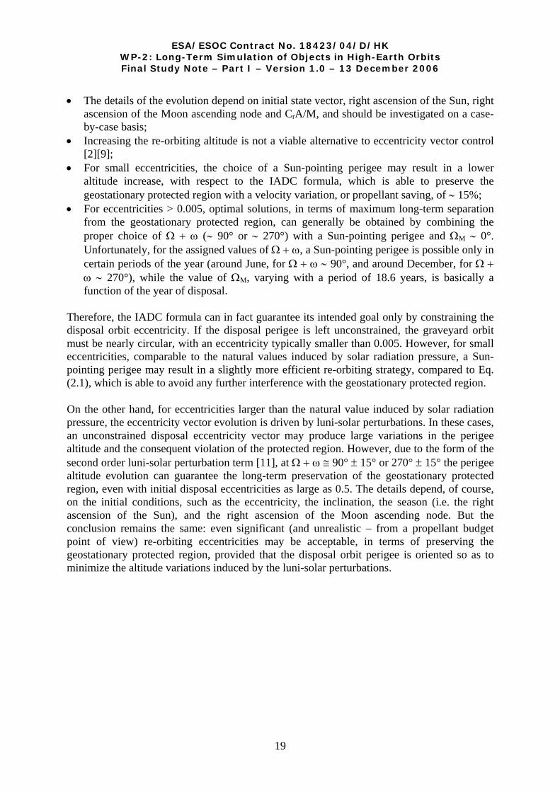
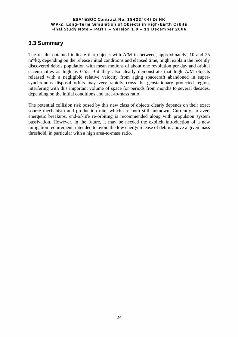
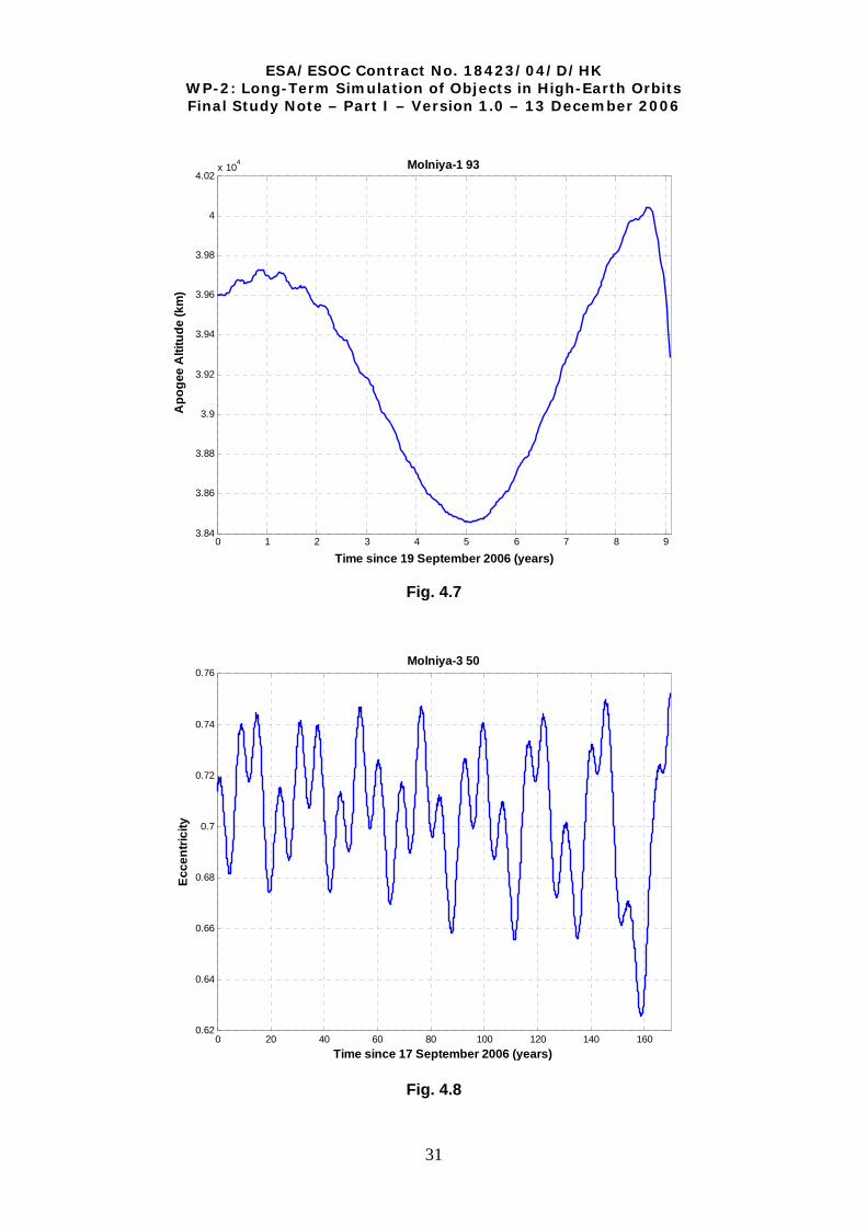
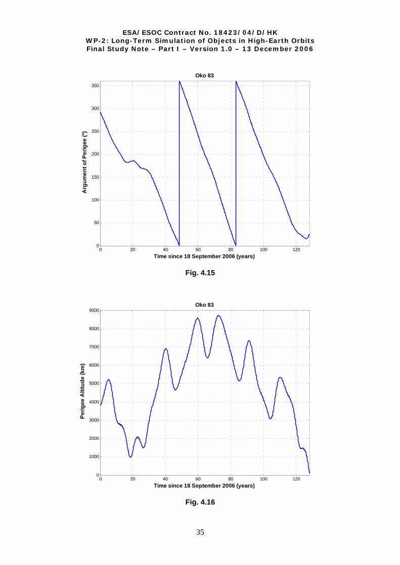
In order to show the typical long-term orbital evolution of Molniya satellites, the results obtained by propagating the orbits of Molniya-1 93 and Molniya-3 50 are presented in the following. Both spacecraft are currently (October 2006) operational, but the propagations were carried out assuming no further orbit keeping maneuvers. This is actually a good approximation, because true Molniya orbits do not require significant maneuvers to be maintained. These two specific satellites were chosen because the first one is a short lifetime case, while the second one is a long lifetime example. The results are summarized in Figures 4.3-4.7 for Molniya-1 93, characterized by a residual lifetime of about 9 years, and in Figures 4.8-4.12 for Molniya-3 50, characterized by a residual lifetime of about 170 years. In both cases, the significant long-term eccentricity variation induced by luni-solar perturbations is evident, translating into large oscillations of apogee and perigee. There are two main components, one with a period of ∼ 7.7 years and the other with a period of ∼ 23 years. The operational perigee altitude can range between 400 and 2500 km. As a consequence of the critical inclination, the argument of perigee librates around 265°-270°, with an amplitude of ± 15-20° and a period of approximately 22 years. This means the perigee remains above the southern hemisphere. The inclination too librates around the critical value, with the same period and an amplitude of ± 1°. Historically, the early warning Oko satellites did not adopt a true Molniya orbit, choosing instead an inclination slightly different from the critical one. This resulted in the need to control actively the orbit with periodic maneuvers, in order to avoid the secular precession of the perigee and maintain it above the southern hemisphere. Another choice typical of Oko orbits was the adoption of higher average perigees. This situation is exemplified by the evolution of the orbit of Oko 83 (Cosmos 2351), launched on 1998 and no longer operational (Figures 4.13-4.17). The range of variation of the significant orbital elements is considerably higher with respect to true Molniya orbits. For instance, the perigee altitude varies between 1000 and 9000 km (Figure 4.16), the eccentricity may decrease below 0.45 (Figure 4.13) and the perigee is affected by a secular precession most of the time (Figure 4.15). More recently, probably to increase the operational lifetime of these satellites, a true Molniya orbit at the critical inclination was, at last, adopted. This is the case, for instance, of the operational spacecraft (as of October 2006) Oko 87 (Cosmos 2422). As for Oko 83, its orbit was propagated with the same model options described at the beginning of this section (Molniya-1 93), setting M = 1250 kg [27] and A = 17 m2 [24]. As shown in Figures 4.18-4.22, assuming no further orbital maneuver, the long-term evolution is similar, apart from the residual lifetime, to that exhibited by authentic Molniya satellites, as Molniya-1 93 and Molniya-3 50.

28


0 1 2 3 4 5 6 7 8 90.68

0.69

0.7

0.71

0.72

0.73

0.74

0.75

0.76Molniya-1 93

Time since 19 September 2006 (years)

Ecce

ntric

ity

Fig. 4.3

0 1 2 3 4 5 6 7 8 963.4

63.6

63.8

64

64.2

64.4

64.6

64.8

65Molniya-1 93


Incl

inat

ion

(°)

Fig. 4.4

29


0 1 2 3 4 5 6 7 8 9240

245

250

255

260

265

270

275

280

285

290Molniya-1 93


Arg

umen

t of P

erig

ee (°

)

Fig. 4.5

0 1 2 3 4 5 6 7 8 90

200

400

600

800

1000

1200

1400

1600

1800

2000Molniya-1 93


Perig

ee A

ltitu

de (k

m)

Fig. 4.6

30


0 1 2 3 4 5 6 7 8 93.84

3.86

3.88

3.9

3.92

3.94

3.96

3.98

4

4.02x 104 Molniya-1 93


Apo

gee

Alti

tude

(km

)

Fig. 4.7

0 20 40 60 80 100 120 140 1600.62

0.64

0.66

0.68

0.7

0.72

0.74

0.76Molniya-3 50


Ecce

ntric

ity

Fig. 4.8

31


0 20 40 60 80 100 120 140 16060.5

61

61.5

62

62.5

63

63.5

64

64.5

65

65.5Molniya-3 50


Incl

inat

ion

(°)

Fig. 4.9

0 20 40 60 80 100 120 140 160230

240

250

260

270

280

290

300Molniya-3 50


Arg

umen

t of P

erig

ee (°

)

Fig. 4.10

32


0 20 40 60 80 100 120 140 1600

500

1000

1500

2000

2500

3000

3500

4000Molniya-3 50


Perig

ee A

ltitu

de (k

m)

Fig. 4.11

0 20 40 60 80 100 120 140 1603.65

3.7

3.75

3.8

3.85

3.9

3.95

4

4.05x 104 Molniya-3 50


Apo

gee

Alti

tude

(km

)

Fig. 4.12

33


0 20 40 60 80 100 1200.4

0.45

0.5

0.55

0.6

0.65

0.7

0.75

0.8Oko 83


Ecce

ntric

ity

Fig. 4.13

0 20 40 60 80 100 12060

62

64

66

68

70

72

74Oko 83


Incl

inat

ion

(°)

Fig. 4.14

34


0 20 40 60 80 100 1200

50

100

150

200

250

300

350

Oko 83


Arg

umen

t of P

erig

ee (°

)

Fig. 4.15

0 20 40 60 80 100 1200

1000

2000

3000

4000

5000

6000

7000

8000

9000Oko 83


Perig

ee A

ltitu

de (k

m)

Fig. 4.16

35


0 20 40 60 80 100 1203.1

3.2

3.3

3.4

3.5

3.6

3.7

3.8

3.9

4

4.1x 104 Oko 83


Apo

gee

Alti

tude

(km

)

Fig. 4.17

0 5 10 15 20 25 30 35 40 450.64

0.66

0.68

0.7

0.72

0.74

0.76Oko 87


Ecce

ntric

ity

Fig. 4.18

36


0 5 10 15 20 25 30 35 40 4561

61.5

62

62.5

63

63.5

64

64.5

65Oko 87


Incl

inat

ion

(°)

Fig. 4.19

0 5 10 15 20 25 30 35 40 45240

250

260

270

280

290

300Oko 87


Arg

umen

t of P

erig

ee (°

)

Fig. 4.20

37


0 5 10 15 20 25 30 35 40 450

500

1000

1500

2000

2500

3000

3500Oko 87


Perig

ee A

ltitu

de (k

m)

Fig. 4.21

0 5 10 15 20 25 30 35 40 453.7

3.75

3.8

3.85

3.9

3.95

4

4.05x 104 Oko 87


Apo

gee

Alti

tude

(km

)

Fig. 4.22

38


4.3 Lifetimes of Molniya and Oko Orbits Since 1990, during the transition period leading to the break-up of the Soviet Union, a total of 34 Molniya [24] and 22 Oko [28] satellites have been launched, as of October 2006. The orbits of the 49 spacecraft not yet decayed [24] have been propagated in order to compile statistics concerning the distribution of their total orbital lifetime, including the operational phase. The trajectories were propagated taking into account the Earth’s geopotential harmonics, up to the 16th order and degree, the third body attraction of the Moon and the Sun, the solar radiation pressure (with Cr = 1.2), including eclipses, and air drag, with the model settings given in Table 1.1. For Molniya satellites, the area-to-mass ratio considered corresponded to a mass of 1600 kg [27] and an average cross-section of 15 m2 [24], while for Oko satellites the mass was set equal to 1250 kg [27] and the average cross-section to 17 m2 [24].

Table 4.2

Distribution of the Total Orbital Lifetime of the Molniya Satellites Launched Since 1 January 1990

Total Orbital Lifetime %

< 15 years 41.2 < 25 years 73.5 < 50 years 94.1 < 75 years 94.1 < 100 years 94.1 < 200 years 97.1 > 200 years 2.9

Table 4.3

Distribution of the Total Orbital Lifetime of the Oko Satellites Launched Since 1 January 1990

Total Orbital Lifetime %

< 15 years 9.1 < 25 years 40.9 < 50 years 54.5 < 75 years 72.7 < 100 years 77.3 < 200 years 86.4 > 200 years 13.6

The results obtained, including in the statistics the 7 Molniya satellites already decayed, are summarized in Tables 4.2 and 4.3. The satellites of the Molniya system are typically characterized by shorter lifetimes, with approximately 3 out of 4 spacecraft leaving the orbit

39


in less than 25 years and 9 out of 10 in less than 50 years (Table 4.2). The Oko satellites, on the other hand, remain in orbit much longer, on the average, with only 4 out of 10 decaying in less than 25 years and a little bit more than one half decaying in less than 50 years. 4.4 Disposal of Satellites in Molniya Orbits Varying by 100 km the altitude of the perigee of a Molniya orbit requires a tangential velocity change (∆V) at the apogee of about 9 m/s. Due to the large perigee excursion induced by the orbital perturbations (see Figures 4.6, 4.11, 4.16 and 4.21), the actual ∆V to be applied in order to re-orbit a spacecraft above LEO, to reduce its orbital lifetime or to cause its direct reentry may vary by a large amount. The best mitigation practice for Molniya-like orbits would be the choice of initial conditions leading to natural decay in a reasonable time, but this is not always possible in practice, due to constellation coverage requirements, as shown in Tables 4.2 and 4.3. De-orbiting or re-orbiting should be therefore considered in the future. However, re-orbiting above LEO presents serious drawbacks. First of all, due to the large perigee height excursion, the ∆V to be applied is highly variable and generally far from negligible. In addition, due to the effects of perturbations, it is not easy to find a minimum re-orbiting altitude able to avoid in the future the crossing of the LEO region. In fact, the perigee of abandoned Molniya satellites may vary its altitude by 3000 km (see Figure 4.11), while that of Oko satellites may vary by 8000 km, or more (see Figure 4.16). Any generalization on Molniya-like orbits may be, then, misleading, concerning a possible disposal above LEO. A better alternative would be the perigee lowering, to reduce the residual lifetime below a certain threshold or to cause a direct reentry. The second strategy would request an additional ∆V, but would be much simpler. In fact, the effectiveness of perigee lowering to reduce the residual lifetime would be assured only by properly taking into account the effects of perturbations. Let assume, for example, the case of Molniya-3 50 (see Figure 4.11). A perigee raise to the altitude of 3000 km, needed to avoid further crossings of the LEO region in the future, would require, as of October 2006, a ∆V of approximately 160 m/s, compared to about 100 m/s to obtain a direct reentry. A lifetime reduction strategy, on the other hand, should take into account the perigee evolution due to orbital perturbations. In this specific case, lowering the perigee at an altitude of 200 km, with a ∆V saving of about 10 m/s with respect to direct reentry, would lead anyway to orbital decay in less than one year, due to the natural perigee evolution. Missing this opportunity time window, on the other hand, would render this strategy not effective for several years to come, because the perigee height will start to increase in 2007, driven by natural perturbations, reaching an altitude of more than 2000 km (see Figure 4.11). The disposal of spacecraft in long lifetime Molniya-like orbits is therefore quite complicated and relatively demanding: it would request a case-by-case analysis. In other words, any generalization could be misleading. However, even for satellites with a lifetime of about 200 years, the dwell time in LEO would be limited to around 50 years.

40


GLOSSARY A/M Area-to-Mass ratio CNR Consiglio Nazionale delle Ricerche (Italian National Research Council) Cr Radiation pressure coefficient (0 ≤ Cr ≤ 2) e Eccentricity ESA European Space Agency ESOC European Space Operations Centre FOP Fast Orbit Propagator GEO GEostationary Orbit GPS Global Positioning System IADC Inter-Agency Space Debris Coordination Committee i Inclination ISTI Istituto di Scienza e Tecnologie dell’Informazione “Alessandro Faedo” LEO Low Earth Orbit (orbital region below the altitude of 2000 km) MEO Medium Earth Orbit, i.e. intermediate in altitude between LEO and GEO SDM Semi-Deterministic Model for space debris mitigation analysis UTC Universal Time Coordinated α Angle between perigee vector and right ascension of the Sun ∆V Velocity change ω Argument of perigee Ω Right ascension of the ascending node ΩM Right ascension of the ascending node of the Moon

41


REFERENCES 1. Analysis of Mitigation Measures Based on the Semi-Deterministic Model, Proposal

presented in response to the ESA Request for Quotation RFQ/3-10961/04/D/HK, ISTI/CNR, Pisa, Italy, 13 September 2004.

2. Anselmo, L. Long-Term Simulation of Objects in High-Earth Orbits, Progress Report No. 1, Work Package 2, ESA/ESOC Contract No. 18423/04/D/HK, ISTI/CNR, Pisa, Italy, 6 December 2005.

3. Inter-Agency Space Debris Coordination Committee (IADC). IADC Space Debris Mitigation Guidelines, IADC-02-01, 15 October 2002.

4. Martin, C. GEO Disposal Orbit Eccentricity, IADC Action Item 22.1 Report, Working Group 4 (Mitigation), IADC-06-04, Version 1.0, 2 November 2006.

5. Martin, C.E., Stokes, P.H., Walker, R., Klinkrad, H. The Long-Term Evolution of the Debris Environment in High Earth Orbit Including the Effectiveness of Mitigation Measures, in: Bendisch, J. (Ed.), Space Debris 2001, Science and Technology Series, A supplement to Advances in the Astronautical Sciences, Vol. 105, Univelt Inc., San Diego, California, USA, pp. 141-154, 2002.

6. Lewis, H.G., Swinerd, G.G., Martin, C.E., Campbell, W.S. The Stability of Disposal Orbits at Super-Synchronous Altitudes, Acta Astronautica 55, 299-310, 2004.

7. Delong, N., Frémeaux, C. Eccentricity Management for Geostationary Satellites During End of Life Operations, in: Danesy, D. (Ed.), Proceedings of the Fourth European Conference on Space Debris, ESA SP-587, ESA Publications Division, Noordwijk, The Netherlands, pp. 297-302, August 2005.

8. Gopinath, N.S., Ganeshan, A.S. Long Term Evolution of Objects in GSO-Disposal Orbit, in: Danesy, D. (Ed.), Proceedings of the Fourth European Conference on Space Debris, ESA SP-587, ESA Publications Division, Noordwijk, The Netherlands, pp. 291-296, August 2005.

9. Anselmo, L. GEO Disposal Orbit Eccentricity, Proceedings of the 24th IADC Plenary Meeting, JAXA, Tsukuba Space Center, Tsukuba, Japan, CD-ROM, April 10-13, 2006.

10. Anselmo, L., Pardini, C. Space Debris Mitigation in Geosynchronous Orbit, Paper PEDAS1-0009-06, Submitted to Advances in Space Research, 13 July 2006.

11. Yaoxiang, J. Effect of Initial Eccentricity Vector on GEO Disposal Orbits, Proceedings of the 24th IADC Plenary Meeting, JAXA, Tsukuba Space Center, Tsukuba, Japan, CD-ROM, April 10-13, 2006.

12. Flury, W., et al. Searching for Small Debris in Geostationary Ring: Discoveries with the Zeiss 1-metre Telescope, ESA Bulletin 104, 92-100, 2000.

13. Schildknecht, T., et al. The Search for Debris in GEO, Advances in Space Research 28, 1291-1299, 2001.

14. Schildknecht, T., et al. Optical Survey for Space Debris in GEO, in: Bendisch J. (Ed.), Space Debris 2001, Sciences and Technology series, A supplement to Advances in the Astronautical Sciences, Vol. 105, Univelt Inc., San Diego, California, USA, pp. 9-21, 2002.

15. Schildknecht, T., et al. Optical Observations of Space Debris in GEO and in Highly-

42

http://scienceserver.cilea.it/cgi-bin/search.pl/GetSearchResults?Any=&Title=&Abstract=&Author=Schildknecht%2C%20T.&JournalTitle=&Past=No+Restriction...&Since=&Start=1&Max=10

http://scienceserver.cilea.it/cgi-bin/sciserv.pl?collection=journals&journal=02731177




Eccentric Orbits, Advances in Space Research 34, 901-911, 2004. 16. Johnson, N.L., et al. History of On-Orbit Satellite Fragmentations, 13th Edition, Orbital

Debris Program Office, JSC 62530, Johnson Space Center, NASA, Houston, Texas, USA, pp. 11-22, May 2004.

17. Pardini, C., Anselmo, L. Long-Term Evolution of Debris Clouds in Geosynchronous Orbit, Proceedings of the 17th International Symposium on Space Flight Dynamics, Keldysh Institute of Applied Mathematics, Space Informatics Analytical Systems (KIA Systems), Moscow, Russia, pp. 56-76, 2003.

18. Pardini, C., Anselmo, L. Dynamical Evolution of Debris Clouds in Geosynchronous Orbit, Advances in Space Research 35, 1303-1312, 2005.

19. Schildknecht, T., et al. Optical Observations of Space Debris in Highly Eccentric Orbits, Oral Presentation PEDAS1/B1.6-0007-04, Space Debris Session, 35th COSPAR Scientific Assembly, Paris, France, 22 July 2004.

20. Liou, J.-C., Weaver, J.K. Orbital Evolution of GEO Debris with Very High Area-to-Mass Ratios, The Orbital Debris Quarterly News 8, Issue 3, 6-7, July 2004.

21. Anselmo, L., Pardini, C. Orbital Evolution of Geosynchronous Objects with High Area-to-Mass Ratios, in: Danesy, D. (Ed.), Proceedings of the Fourth European Conference on Space Debris, ESA SP-587, ESA Publications Division, Noordwijk, The Netherlands, pp. 279-284, August 2005.

22. Pardini, C., Anselmo, L. Long-Term Evolution of Geosynchronous Orbital Debris with High Area-to-Mass Ratios, 25th International Symposium on Space Technology and Science, Paper 2006-r-2-10, CD-ROM, The Organizing Committee of the 25th ISTS and the Japan Society for Aeronautical and Space Sciences, Kanazawa, Japan, June 2006.

23. Grimwood, T. The UCS Satellite Database, Union of Concerned Scientists (UCS), Cambridge, Massachusetts, USA, http://www.ucsusa.org/satellite_database, 21 Sept. 2006.

24. Space Track – The Source for Space Surveillance Data. Space Track Organization, USA, http://www.space-track.org/perl/login.pl, October 2006.

25. Anselmo, L. Spie dal Cielo, le Stelle 2, No. 4, 42-55, February 2003. 26. Anselmo, L. Lo Spionaggio dei Segnali dallo Spazio, Presentazione alla Giornata di

Studio “Echelon e la Sicurezza nel Sistema-Mondo”, Dipartimento di Studi Internazionali, Facoltà di Scienze Politiche, Università di Milano, Milano, 27 May 2004.

27. Wade, M. Encyclopedia Astronautica, USA, http://astronautix.com/index.html, October 2006.

28. Krebs, G. Gunter’s Space Page, Germany, http://www.skyrocket.de/space/space.html, October 2006.

43

http://scienceserver.cilea.it/cgi-bin/sciserv.pl?collection=journals&journal=02731177


http://www.cosis.net/abstracts/COSPAR04/01566/COSPAR04-A-01566-1.pdf

http://www.copernicus.org/COSPAR/COSPAR_paris.html

http://www.copernicus.org/COSPAR/COSPAR_paris.html

http://www.ucsusa.org/satellite_database

http://www.space-track.org/perl/login.pl

http://astronautix.com/index.html

http://www.skyrocket.de/space/space.html

long-term simulation of objects in high-earth...

Documents