long term radiometric calibration: can we extend ... term radiometric calibration: can we extend...
TRANSCRIPT

Long Term Radiometric Calibration: Can We Extend Consistent
Calibration Parameters From Landsats 7 & 5 Back Through
Landsats 1-4 MSS?David AaronDennis HelderJim DewaldLarry LeighRaj Bhatt, Sirish Uprety, Rimy Malla,
Cody Anderson, Dan Morstad
Landsat Science Team Meeting: Reston, VA July 15-17, 2008

Motivation:Over 35 years of data
Graphic from: landsat.usgs.gov/about_mission_history.php
Landsat Missions Timeline

Data from Landsat 7(ETM+) and Landsat 5(TM) are trended and processed using a consistent system (IAS projects).
An archive exists from 6 Landsat sensor systems:– Landsats 1-3
• RBV• MSS
– Landsats 4-5• MSS• TM
– Landsat 7• ETM+
With the launch of OLI the long term data base will extend into the future.

As we extend earth observation into the future, can archived Landsat data be reprocessed to provide a better data continuum?
SDSU is taking its experience base in radiometric calibration to:
•Evaluate the viability of extending the Landsat 5 and 7 calibration base back through the predecessor Landsat sensor systems.•Establish a basis for an IAS system to trend these predecessor systems.•Sadly we can’t use our vicarious calibration technique
•Time machine?

MSS Calibration Plan Outline• L5 MSS Calibration
– Calibrate to L5 TM through coincident scenes– Develop trend through use of invariant sites– Develop trend through use of internal cal wedge data
• L4 MSS Calibration– Calibrate to L4 TM through coincident scenes– Calibrate to L5 MSS through coincident or near-coincident scenes– Develop trend through use of invariant sites– Develop trend through use of cal wedge data
• L3 MSS Calibration– Calibrate to L4 MSS through coincident or near coincident scenes
• Note: this is likely the highest risk point in the process!– Potential cross-calibration to L4 TM through coincident or near coincident scenes– Develop trend through use of invariant sites– Develop trend through use of cal wedge data
• Landsat 2 MSS Calibration– Calibrate to L3 MSS through coincident or near coincident scenes– Develop trend through use of invariant sites– Develop trend through use of cal wedge data
• Landsat 1 MSS Calibration– Calibrate to L2 MSS through coincident or near coincident scenes– Develop trend through use of invariant sites– Develop trend through use of cal wedge data

‘Back-calibrate’ via:
L5 TM L5 MSS
L5 MSS L4 MSS
L4 MSS L3 MSS
L3 MSS L2 MSS
L2 MSS L1 MSS
Question: Is there sufficient data to follow this data chain?

Archive Data Overlap TimelineN
umbe
r of S
cene
s
Sensor Overlap Timeline
0
10000
20000
30000
40000
50000
60000
1972
1973
1974
1975
1976
1977
1978
1979
1980
1981
1982
1983
1984
1985
1986
1987
1988
1989
1990
1991
1992
1993
1994
Year
L5L4L3L2L1
Num
ber o
f Sce
nes

Overlap TimelineYear L1 L2 L3 L4 L51972 241001973 538841974 400471975 13138 397841976 9633 414241977 6824 447741978 101 18868 258581979 12801 175721980 9280 187241981 19257 81421982 1481 16348 60581983 872 224601984 11141 262041985 348 284471986 423 407801987 464 354691988 3612 112171989 4687 65061990 1377 70591991 116 91741992 2932 80431993 01994 1
Total Scenes 147727 187669 87516 53619 172900

L5 Coincident Scenes (Total 32318)
3957
4833
8824
7854
17211017 796
1700 1616
0
1000
2000
3000
4000
5000
6000
7000
8000
9000
10000
1984 1985 1986 1987 1988 1989 1990 1991 1992Year
L5
No.
of S
cene
s
Timeframe of L5 TM/MSS Coincident Scenes

L5/L4 Near Coincident MSS Scenes
• The shortest period between any two near-coincident scenes of L4 and L5 MSS is 8 days.
• Several good quality near-coincident scenes from White Sands, Sonoran Desert, Railroad Valley, Ivanpah Playa, and Rogers Dry lake exists for Cross-Calibrating L5 MSS to L4 MSS.
White Sands (P33R37)
L4 Scene ID L5 Scene IDLM40330371984310AAA03 LM50330371984302AAA03 LM40330371985056AAA03 LM50330371985048AAA03 LM40330371992188AAA03 LM50330371992180AAA03

L5/L4 Near Coincident MSS Scenes (contd.)
L4 Scene ID L5 Scene IDLM40380381992159AAA03 LM50380381992183AAA03
Sonoran Desert (P38R38)
Railroad Valley(P40R33)
L4 Scene ID L5 Scene IDLM40400331992205AAA03 LM50400331992213AAA03
Ivanpah Playa (P39R35)
L4 Scene ID L5 Scene IDLM40390351986277AAA03 LM50390351986285AAA03LM40390351986309AAA03 LM50390351986317AAA03

Example: Sonoran Desert L3/L4 MSSCross Cal images
L3 MSS• ID: LM30410381982365AAA03• Cloud Cover: 90% Qlty: 9• Date: 1982/12/31• Sun Elevation: 27• Sun Azimuth: 147
L4 MSS• ID: LM40380381983022AAA03• Cloud Cover: 10% Qlty: 9• Date: 1983/1/22• Sun Elevation: 29• Sun Azimuth: 144
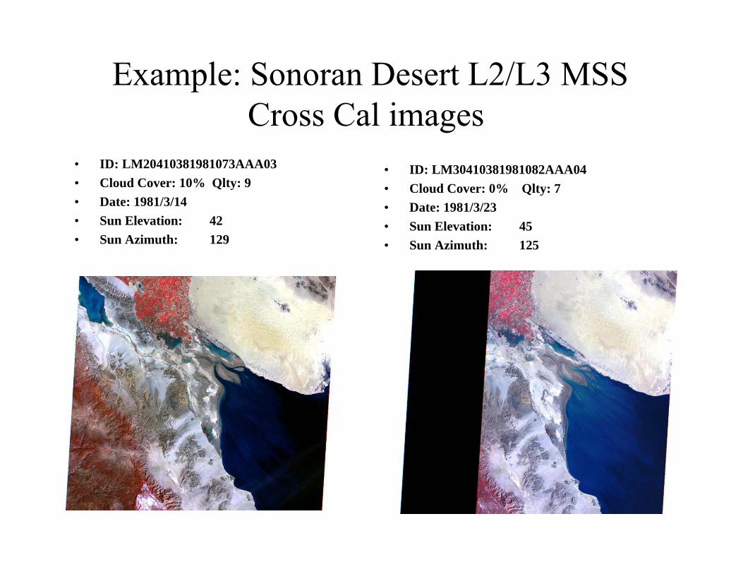
Example: Sonoran Desert L2/L3 MSS Cross Cal images
• ID: LM20410381981073AAA03• Cloud Cover: 10% Qlty: 9• Date: 1981/3/14• Sun Elevation: 42• Sun Azimuth: 129
• ID: LM30410381981082AAA04• Cloud Cover: 0% Qlty: 7• Date: 1981/3/23• Sun Elevation: 45• Sun Azimuth: 125

Example: Sonoran Desert L1/L2 MSSCross Cal images
• ID: LM10410381975348AAA01• Cloud Cover: 10% Qlty: 4• Date: 1975/12/14• Sun Elevation: 25 • Sun Azimuth: 143
• ID: LM20410381975357AAA01• Cloud Cover: 10% Qlty: 4• Date: 1975/12/23• Sun Elevation: 26 • Sun Azimuth: 147

Scene availability summary
• Significant number of TM/MSS coincident scenes from various calibration sites exists (particularly for L5).
• Sufficient near-coincident scenes are available for cross-calibration of L5 to L4 MSS, L3 to L2 MSS, and L2 to L1 MSS.
• Cross-calibration of L4 MSS to L3 MSS is somewhat critical (very few near-coincident scenes are available in the EROS archive)

Our partners at ESA

Libya 4 scenes at ESA
• Some additional Libya 4 scenes of Landsat 1-7 are available at ESA that are not in USGS archive.
• As per information in ESA’s website, they have L0R data available for MSS sensors.
• Landsat 2– 14 Libya 4 scenes available for Landsat 2 from 1976 to 1981 (at least
one scene every year). – The L0R data of these could be the potential source to investigate the
lifetime trend of this sensor.• Some scenes exist for other sensors too which along with the
scenes available in USGS archive could be useful for cross-cal of MSS sensors.
• Received an initial set of scenes which are in the process of being analyzed.

• There are many instances where L5 imaged our known invariant test sites with TM and MSS instruments simultaneously; thus, opening the opportunity of Cross-calibrating L5 MSS against L5 TM using a simultaneous scene-pair based approach
• The shortest period between any two near-coincident scenes of L4 and L5 MSS is 8 days
• The MSS-A data available is in calibrated DNs (Qcal)
L5 TM L5 MSS
L5 MSS L4 MSS
Notes on applying the Pseudo-Invariant Calibration Site (PICS) technique

Region of Interest
• Twelve good quality, cloud free coincident TM and MSS scenes (1984 to 1987) from Libya 4 test site were used for this study
• ROI : 1090*630 pixels rectangle on Libya 4 MSS scene
• The sensitivity to possible misregistration was checked by shifting the ROI up and down; left and right (up to 5 MSS pixels, one at a time) and mean DN was calculated for the specified ROI in every shift of the ROI
• Very low standard deviation (less than 1%) of the Mean DNsindicates misregistration should not pose a significant problem for Libya 4 scenes
L5 TM L5 MSS

Spectral Considerations
In band radiance is a function of:• specified bandwidth (BW)• system relative spectral response (RSR)

In-band Radiance to Spectral Radiance Conversion: Bandwidth considerations
FWHM
1
λ
0.5
Different specifications of bandwidth– Nominal BW– FWHM (Markham and Barker, 1983)– Equivalent Rectangular Bandwidth (ERBW)– Quadratic moment BWs (Palmer, 1984; Malila
and Anderson, 1986)
Band Nominal BW FWHM BW ERBW QMBW
1 0.100 0.109 0.106 0.1162
2 0.100 0.0937 0.089 0.0988
3 0.100 0.1099 0.099 0.1163
4 0.300 0.2263 0.221 0.2752
Possible specifiers for effective BWs for L5 MSS bands (in micrometers)

Dissimilar RSR Profiles: A key concern
• None of the four bands match closely in their RSR profiles, indicating that the two sensors may produce different results while looking at the same ground target
• Effect of Spectral Band Difference is scene specific, and we need to know the spectral signature of target as well to find the Spectral Band Adjustment Factors (SBAFs)
TMMSS
MSS TM FOM
B1 B2 0.635B2 B3 0.708B3 B4 0.182B4 B4 0.328
Spectrally best matching pairs
Figure of Merit (FOM)
This indicates which bands of two different sensing instruments should respond more similarly to ground targets as compared to others

Spectral Band Adjustment Factors (SBAFs)R(λ): Band specific RSR ProfileL(λ): Upwelling Radiance of Target
∫∫=
TMTM
MSSMSS
BWdLR
BWdLRSBAF
/)(
/)(
,
,
λ
λ
λλ
λλ

Need RSR’s and Appropriate Surface Spectral Signature (SSS).
RSR’s• TM• MSS
– L5 and L4 easy – L3, L2, L1 analog only
• MSS Radiometric Calibration Handbook (RCH) 1993• FindGraph
SSS for desert site

Spectral Signature of Libya 4Hyperion to the rescue
(MSS Bands indicated)
5 June, 200728 June, 2007
L5 MSS Band 4 is susceptible to water vapor content in the atmosphere, whereas the corresponding band in L5 TM is not.

Cross-calibration procedure• Mean of all pixels (calibrated DNs, Qcal) within specified region of interest
was calculated from MSS data for each band
• LMIN and LMAX values (W/m2 sr um) for L5 MSS were calculated from historical RMIN and RMAX values (W/m2 sr) found in MSS RCH by multiplying with a factor of 10 and dividing by the Nominal BW (private communication with Brian Markham) of respective bands.
• These LMIN and LMAX values were used as scaling factors to convert Qcal(for MSS) to band average spectral radiance values.
• Corresponding TM scenes were processed on TMIAS 8.0.2, and mean spectral radiance values for the ROI were found directly using L1R product data.
• The ratio of TM and MSS radiance values for best matching bands were multiplied by corresponding Spectral Band Adjustment Factors (SBAFs), and plotted against DSL.
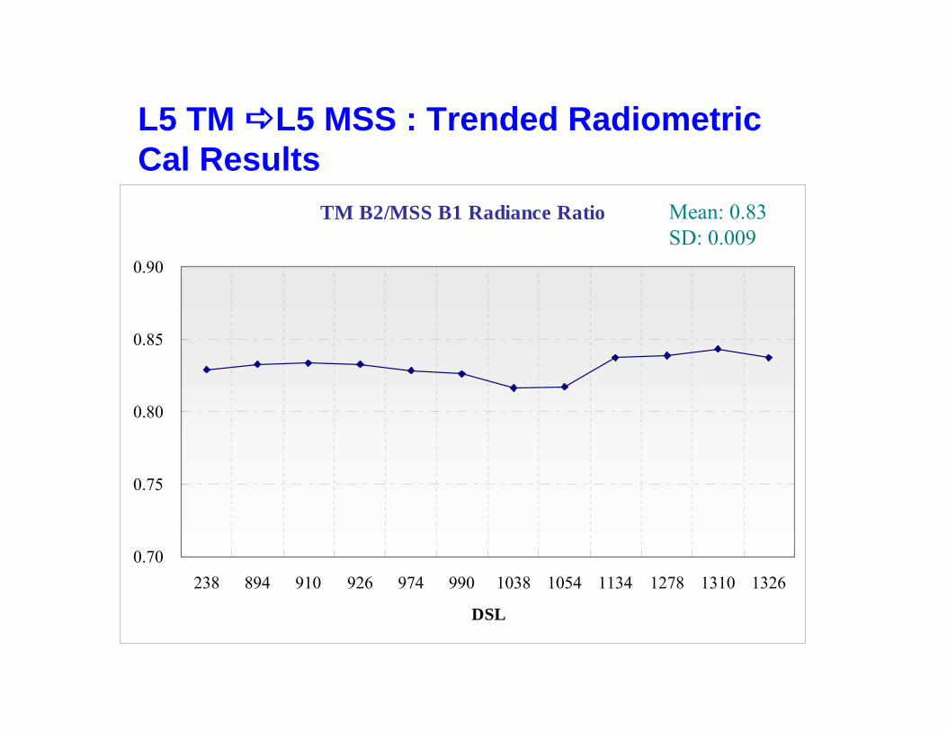
TM B2/MSS B1 Radiance Ratio
0.70
0.75
0.80
0.85
0.90
238 894 910 926 974 990 1038 1054 1134 1278 1310 1326
DSL
Mean: 0.83SD: 0.009
L5 TM L5 MSS : Trended Radiometric Cal Results

TM B3/M SS B2 Radiance Ratio
0.80
0.85
0.90
0.95
1.00
1.05
238 894 910 926 974 990 1038 1054 1134 1278 1310 1326
D SL
Mean: 0.93SD: 0.025
L5 TM L5 MSS : Trended Radiometric Cal Results

T M B 4 /M S S B 3 R a dia nce R a tio
0.85
0.90
0.95
1.00
1.05
1.10
238 894 910 926 974 990 1038 1054 1134 1278 1310 1326
D SL
Mean: 0.95SD: 0.042
L5 TM L5 MSS : Trended Radiometric Cal Results

T M B 4 /M S S B 4 R a dia nc e R a tio
0.80
0.85
0.90
0.95
1.00
1.05
1.10
238 894 910 926 974 990 1038 1054 1134 1278 1310 1326
D SL
Mean: 0.95SD: 0.026
L5 TM L5 MSS : Trended Radiometric Cal Results

Summary: Cross-calibration results normalized to L5 TM
Sensor MSS B1 /TM B2
MSS B2 /TM B3
MSS B3 /TM B4
MSS B4 /TM B4
L5 TM 1.00 1.00 1.00 1.00L5 MSS 1.08 1.14 0.99 1.33
Sensor MSS B1 /TM B2
MSS B2 /TM B3
MSS B3 /TM B4
MSS B4 /TM B4
L5 TM 1.00 1.00 1.00 1.00L5 MSS 1.20 1.08 1.05 1.05
Initial round of test results (using FWHM BWs)
New Results (using Nominal BWs)

• Near-coincident scene pairs from White Sands, Ivanpah Playa, RRV, and Sonoran Desert used for this study
• Nominal passbands were used to convert In-Band radiance to Spectral radiance units
• What about RSR’s?
L5 MSS L4 MSSPilot radiometric cross cal

RSR profiles of L4 and L5 MSS bandsL4L5
• Life is good: Very similar RSR profiles (SBDE consequently neglected)

What about geolocation?
• A particular object on the ground may not have the same pixel coordinates in the near coincident scenes taken by different satellites
• The following steps were followed to ensure the best possible co-location:– Find coordinates of three geographical reference points (Highway
intersection, runway edges, buildings, etc) on each of the scene pairs and determined their offset values.
– Offset values were not the same for different reference points, indicating
• Translation• Rotation• Shear/Skew
– Used standard transforms (Affine) to obtain best co-location

Radiometric Evaluation Formulation• Convert calibrated DNs to TOA radiance using appropriate rescaling
gains (standard Lmin, Lmax, Qcal conversion)
• Convert TOA radiance to TOA reflectance to remove the cosine effect of different solar zenith angles and compensate for different values of exo-atmospheric solar irradiance
ρi* =π Lλi
*ds2/(Eoicosθ)
where, Eoi: Exo-atmospheric solar irradiance
• Plot L4 MSS reflectance against L5 MSS reflectance for differentROIs
• Least square fit the data in each band and find cross cal Gain and biases as the coefficients of the linear fit.

Band 1 Reflectance plot
y = 0.8921x + 0.0033R2 = 0.9831
0.00
0.05
0.10
0.15
0.20
0.25
0.00 0.05 0.10 0.15 0.20 0.25
White Sands Yuma
RRV Linear (Line Fit)
L5 MSS Reflectance
L4 MSS Reflectance
L4 to L5 MSS TOA Reflectance Ratio % Difference in Reflectance EstimatesROI White Sands Sonoran Desert RRV White Sands Sonoran Desert RRV
1 0.954 0.913 0.885 4.47 8.71 11.552 0.923 1.014 8.95 1.373 0.933 0.914 1.99 8.56
Average: 6.51
Band 1 Summary
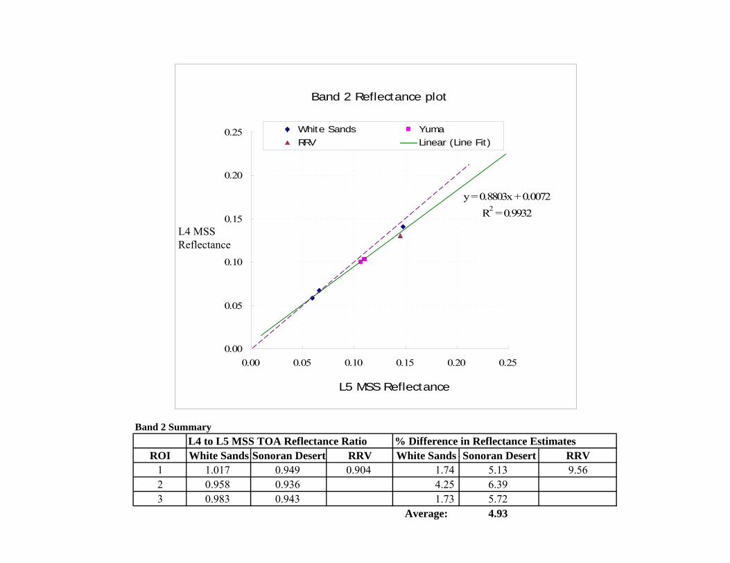
Band 2 Reflectance plot
y = 0.8803x + 0.0072R2 = 0.9932
0.00
0.05
0.10
0.15
0.20
0.25
0.00 0.05 0.10 0.15 0.20 0.25
White Sands YumaRRV Linear (Line Fit)
L5 MSS Reflectance
L4 MSS Reflectance
L4 to L5 MSS TOA Reflectance Ratio % Difference in Reflectance EstimatesROI White Sands Sonoran Desert RRV White Sands Sonoran Desert RRV
1 1.017 0.949 0.904 1.74 5.13 9.562 0.958 0.936 4.25 6.393 0.983 0.943 1.73 5.72
Average: 4.93
Band 2 Summary

Band 3 Reflectance plot
y = 0.9204x + 0.0049R2 = 0.9925
0.00
0.05
0.10
0.15
0.20
0.25
0.00 0.05 0.10 0.15 0.20 0.25
White Sands Yuma
RRV Linear (Line Fit)
L5 MSS Reflectance
L4 MSS Reflectance
L4 to L5 MSS TOA Reflectance Ratio % Difference in Reflectance EstimatesROI White Sands Sonoran Desert RRV White Sands Sonoran Desert RRV
1 1.036 0.961 0.942 3.64 3.94 5.782 0.989 0.952 1.07 4.783 0.974 0.949 2.63 5.14
Average 3.85
Band 3 Summary

Band 4 Reflectance plot
y = 0.9075x + 0.0092R2 = 0.8959
0.00
0.05
0.10
0.15
0.20
0.25
0.00 0.05 0.10 0.15 0.20 0.25
White Sands Yuma
RRV Linear (Line Fit)
L5 MSS Reflectance
L4 MSS Reflectance
L4 to L5 MSS TOA Reflectance Ratio % Difference in Reflectance EstimatesROI White Sands Sonoran Desert RRV White Sands Sonoran Desert RRV
1 1.118 0.941 0.971 11.82 5.88 2.912 1.082 0.915 8.22 8.473 1.041 0.911 4.14 8.91
Average: 7.19
Band 4 Summary

Conclusions: L5 TM to L5 MSSL5 MSS to L4 MSS
• The average radiance estimates for L5 MSS bands 2, 3, and 4 agree within 8% to the best matching L5 TM bands after accounting for spectral band difference effects.
• Cross-calibration result for L5 MSS band 1 (using Nominal BW for MSS to convert In-band Radiance to Spectral units) is not good (agrees within 20%).
• The reflectance estimates of L4 MSS agree with those of L5 MSS to within 7% for Band 1, 5% for Band 2, 4% for Band 3,and 8% (was 9% with FWHM BW) for Band 4.
• L4 and L5 MSS calibration approaches seems to be consistent within 8%.• More scenes and BRDF considerations may help in analysis.

What about L1-L3?
• Need to understand the scene data– Format– Level of product
• Calibration applied?
– PM and silicon diode
• Calibration lamp (‘wedge data’)• Instrument stability as measured by wedge
– ‘short term’ stability

Systems background for Landsat 1 MSS• Landsat 1 MSS bands 1, 2, and 3 were already calibrated, whereas band 4 was
left uncalibrated.• Looking only at the calwedge lifetime trends, it is hard to rigidly distinguish
the detector vs. lamp stability over lifetime as there is no common lifetime trends among the detectors.
– Trends reflect the performance of either detector or lamp, or both.• One possible way to distinguish the detector vs. lamp stability is to get the
lifetime detector response from two different sources:– Lamp (calwedge lifetime trends) and– Invariant site Approach
• For L1, there exists the potential to implement the two approaches since band 4 was left uncalibrated postlaunch.
• Two sources of MSSX data: WBVT and GSFC– WBVT/MSSX band 4 data decompressed to 0-127 when it should not have been.– Band 4 data from WBVT/MSSX had calibration applied to it by WBVT/APGS
software.– Band 4 data from GSFC/MSSX has dynamic range of 0-63.

Landsat 1 MSS Stability and Calibration
• Study Landsat 1 MSS instrument stability and trend.• Investigate the calibration consistency of Landsat 1 MSS
bands 1, 2 , and 3.• Evaluate Post Launch Band 4 Calibration based on Gains and
Offsets from cal-wedge data

Pilot Study Using Sonoran PICS1. 104103800722389042. 104103800722569043. 104103800722749044. 104103800723109045. 104103800723649046. 104103800730889047. 104103800731069048. 104103800731429049. 1041038007316090410. 1041038007319690411. 1041038007328690412. 1041038007404790413. 1041038007406590414. 1041038007410190415. 1041038007415590416. 10410380074173904
17. 1041038007419190418. 1041038007422790419. 1041038007504290420. 1041038007515090421. 1041038007529490422. 1041038007533090423. 1041038007607390424. 1041038007610990425. 1041038007614590426. 1041038007618190427. 1041038007623590428. 1041038007628990429. 1041038197715490430. 1041038197726290431. 10410381977298904
* Not appropriate for Invariant Site Approach due to Cloud over ROI
* WBVT Scenes
• Cal-wedge data extraction was done with28 scenes (from SN 1-28)
• Scenes 29-30 have corrupted data forband 1
ROI(250*250)
• The ROI taken is the best invariant region in Sonoran site as per the Small Invariant Site study done at SDSU
• Affine transformation method used to geolocate the ROI in every scene.
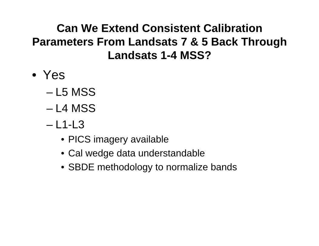
Can We Extend Consistent Calibration Parameters From Landsats 7 & 5 Back Through
Landsats 1-4 MSS?
• Yes– L5 MSS– L4 MSS– L1-L3
• PICS imagery available• Cal wedge data understandable• SBDE methodology to normalize bands

What next?• Complete data format validation for L1-L3 MSS• Complete cal lamp based stability validation• Complete PICS stability validation• Work back from L4 MSS to
– L3 MSS-L2 MSS
-L1 MSS• Continue work with EROS Data Center to develop MSIAS
ISSUES:•Per detector calibration
•Different RSR’s due to filter variations•Images available have been resampled so detector info lost
•Band difference interpretation/education

BACKUP SLIDES

Timeframe of L4 TM/MSS Coincident Scenes
L4 Coincident Scenes (Total 2055)
153
291
19 0 0 0
539
686
4013
314
0
100
200
300
400
500
600
700
800
1982 1983 1984 1985 1986 1987 1988 1989 1990 1991 1992Year
L4
No.
of S
cene
s

Atmospheric Transmittance