long-term ground movement prediction by monte carlo...
TRANSCRIPT

Long-Term Ground Movement Prediction by Monte Carlo Simulation Mark J. Carlotto1
General Dynamics Advanced Information Systems
Abstract A method is described for predicting the long-term movement of people on the ground, either on foot or driving vehicles, as a function of the terrain, weather, behavior, and situation (context). It uses the results of statistical simulations to estimate location probability distributions of where a vehicle or person may go in a given amount of time. Several applications are discussed including detecting possible gaps in sensor coverage, route planning, and mobile communications routing. Key words: Ground vehicle movement prediction, Intelligence Preparation of the Battlefield (IPB), mobility analysis, F* algorithm, dynamic programming, Monte Carlo simulation.
1. Introduction
Predicting the movement of ground vehicles (and people) is important in a variety of applications including target tracking, sensor management, resource allocation, collision/obstacle avoidance, route planning, search and rescue, and others. Some involve projecting movement over relatively short time intervals (less than a few minutes), while others involve predictions out tens of minutes or more. Kinematic (target dynamic) models can be used for short-term prediction (less than a few minutes) but are not effective in predicting ground movement over longer time horizons (tens of minutes to an hour into the future). Over the long term, ground movement is constrained fundamentally by mobility. Road class, terrain type, slope, weather, and other physical factors limit maximum speed, which determines the area that can be reached in a given period of time. What a person or vehicle is doing (behavior) defines where in the reachable area one would expect to find it. For example, is a vehicle moving to/away from known sites, following familiar routes, attempting to avoid detection, etc. These factors can be used to prioritize the reachable area by means of spatial probabilities conditioned on a set of assumed behaviors. Section 2 reviews previous work related to ground movement prediction, and discusses the analytic utility of long-term prediction in a closed loop intelligence surveillence and reconnaissance (ISR) control process. Section 3 describes a method for predicting long-term movement that uses the results of statistical simulations to estimate location probability distributions of where a vehicle or person may go in a given amount of time. Several applications are briefly discussed in Section 4 including detecting potential gaps in sensor coverage, route planning, and mobile communications routing.
2. Previous Work
Long-term prediction is an important part of Intelligence Preparation of the Battlefield (IPB), and was initially developed within that community. Motivated by the limited accuracy and speed of manual terrain analysis (Appendix A), automated tactical decision support systems combining terrain, weather, threat, and military organization/tactical data were first developed in the mid 1980s1. The Army’s All-Source Analysis System (ASAS)2 followed in the 1990s. The first movement prediction capability was the Tactical Movement Analysis (TMA) component in ASAS. TMA used a version of Dijkstra's algorithm3 to combine terrain data (elevation and features), weather, ground forces locations, and movement characteristics into two cost surfaces – one representing movement times and the other movement directions. Subsequent processing of the cost surfaces produced isochronal (fixed time) contours and shortest paths.

A different approach to movement prediction was developed over roughly the same period, and is the basis of the Movement Projection (MP) component in the Joint Tactical Analysis Toolkit (JTAT)4. This approach used a Markov-Bayes predictor to project current enemy locations into the future based on behavior and terrain factors. Target state (location and activity) at a future time
!
x(t + N"t) are determined recursively from the current state
!
x(t) . Operational factors (terrain limitations, move-stop-move behavior, etc.) are represented statistically as transition probabilities,
!
p[x(t + "t) | x(t)] that vary in space as a function of the terrain, and over time as target behavior changes. The projected location of a target is described by a location probability distribution (LPD). Peaks in the LPD indicate likely locations of the target. As the prediction time out increases, the uncertainty in spatial location increases as the initial state estimate diffuses in space (Fig. 1). Predictions out to time
!
T = N"t require
!
N iterations of the algorithm, each of which involves convolving a transition probability kernel with the LPD.
t=0 t=∆t t=2∆t t=10∆t
Fig. 1 Evolution of LPD as a function of time in Markov-Bayes predictor
A software system known as Predict was developed for analyzing long-term ground vehicle movement in support of dynamic sensor management and other ISR planning activities in DARPA’s Dynamic Tactical Targeting (DTT) system5. The system predicts future locations of vehicles moving through road networks. A vehicle’s motion is modeled statistically by the mean (µ) and standard deviation (σ) of its speed as a function of vehicle type and road category. The F* algorithm6 computes two minimum travel time arrays to all locations in the network from the current location: one assuming the vehicle is moving at a minumum speed (µ-Nσ), the othe assuming the vehicle is moving at a maximum speed (µ+Nσ), where the number of standard deviations N is a parameter. The area reachable in a given time is determined by thresholding these arrays. Taking the exclusive-or of the two arrays results in a set of predicted intervals along the road network that can be reached in a given amount of time7.
Fig. 2 ISR target tracking control loop
Going beyond static IPB analysis Predict operates within a closed-loop control system (Fig. 2). Various delays or latencies exist in closed-loop ISR systems, such as the time to position/reposition sensors, to collect and process data, etc. The role of Predict is to project the location of targets far enough into the future in order to compensate for these delays. If
!
T is the system latency, and
!
"v is the uncertainty in the speed of a vehicle being tracked, the accuracy of a prediction
!
"x = "vT depends on the latency. In Appendix B it is shown that kinematic prediction techniques, which take advantage of short-term correlations in vehicle motion, cannot accurately predict out beyond a couple of minutes. In order to
Sensor
ManagementPrediction
Current target states
(location, speed)Predicted target
locations
Tracking Sensors
Collection PlanReports, tracks,...
maintain long-term tracks on targets, knowledge of future target locations tens of minutes into the future is needed to determine if the current collection plan is sufficient to provide the data required to maintain track on a target. Predicted target locations that are not adequately covered by the current collection plan must be determined so that the collection plan can be modified accordingly. Two important track metrics are track length, and the probability of correct identification (PID). Loss of track reduces track length and PID. Results over three different areas demonstrated greater than a 30% increase in average track length, and a 20-50% increase in PID when long-term (terrain-based) prediction was used together with short-term (kinematic) prediction. Where the computational complexity of a Markov-Bayes predictor is grows with the length of the time horizon (
!
N =T /"t ), that of the F* is constant over time. Although the F* algorithm can be several orders of magnitude more compute-efficient than Markov-Bayes, what it lacks is the ability to estimate LPDs, which provide a finer-grained estimate of where vehicles are likely to be located.
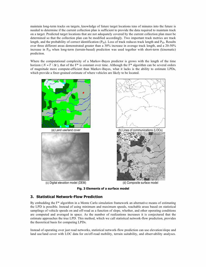
(a) Land use/land cover (b) Lines of communications (LOCs)
(c) Digital elevation model (DEM) (d) Composite surface model
Fig. 3 Elements of a surface model
3. Statistical Network-Flow Prediction
By embedding the F* algorithm in a Monte Carlo simulation framework an alternative means of estimating the LPD is possible. Instead of using minimum and maximum speeds, reachable areas based on statistical samplings of vehicle speeds on and off-road as a function of slope, whether, and other operating conditions are computed and averaged in space. As the number of realizations increases it is conjectured that the estimate approaches the true LPD. This method, which we call statistical network-flow prediction, provides the theoretical basis for computing LPDs. Instead of operating over just road networks, statistical network-flow prediction can use elevation/slope and land use/land cover with LOC data for on/off-road mobility, terrain suitability, and observability analyses.

Terrain and feature data are used to build a 2.5-D surface model over the area of interest. A surface model (Fig. 3d) is created by combining land cover (a) and LOC data (b) with a digital elevation model (c). The F* algorithm computes the minimum travel time map from a given starting point to all points on the surface in parallel. The speed across a node depends on the nature of the surface (i.e., land use/land cover, slope, etc.). It also varies within a surface type, based on micro-terrain, driving behavior (e.g., start-stop), and other random factors, which are not directly observable. These random factors can be described statistically by motion models that give the distribution of speeds of a vehicle are conditioned on the surface type (Fig. 4). Uncertainty in speed results in uncertainty in predicted location, which is represented by the 2-D LPD.
LPDs are estimated using a Monte Carlo simulation that randomly samples from the object’s location and speed probability distributions and averages. Fig. 5 illustrates a simulation over the above area. The process can be summarized as follows:
1) For each cell, generate a random speed from the vehicle speed distribution corresponding to the road/terrain class/slope of the cell
2) Compute the local (random) travel time (cell size/speed) for each cell from the random velocity (a)
3) Determine the total travel time from the starting point to all cells using the F* algorithm (b)
4) Mark cells that can be reached in time t < T by thresholding the travel time array (c). This is one
realization of the underlying random process. 5) Repeat the above steps 1) to 4) N times. Each repesents how far the vehicle can travel at a
randomly generated speed. 6) Count the frequency of occurrence of reachable cells and normalize (d).
(a) Unit travel time array (b) Total travel time array from current location
(c) Reachable area (t < 15 min.) (d) Estimated LPD @ T=15 min. for 10 Monte Carlo runs
Fig. 5 Monte Carlo simulation example
0.00
0.20
0.40
0.60
0.80
0 5 10 15 20
Speed (m/sec) Fig. 4 Vehicle motion model on roads. Different distributions describe speed
off road.
High
Low

Fig. 6 shows the resultant LPD. The highest probability locations are along roads. Off-road locations have probabilities 50-80% below that of road locations; travel is prohibited in river and high slope areas.
(a) Isometric plot of the LPD
(b) False color display of LPD where highest probabilities (in red) are along roads
Fig. 6 Views of estimated LPD
4. Applications
LPDs can be combined with other kinds of information in simulation framework8 to generate various prediction products. Sensor models describe the flight path, field of view, and other parameters for estimating the probability of observing a projected vehicle at a particular location by a sensor over a given time horizon. Observability is used to estimate track/fusion performance, and to detect possible gaps in projected sensor coverage. Fig. 7a shows the observability map for a sensor 10° above the horizon at an azimuth 170-190°. Areas of low observability are in valleys shadowed by higher terrain to the south. Observability maps combined with LPDs indicate possible sensor coverage gaps (Fig. 7b). Regions in red are those likely to be reached by the vehicle in T=15 minutes that will not be observable.
(a) Observability map (b) Coverage gap probability map
Fig. 7 Coverage gap product to support sensor management
Multiple object predictions can be used to solve route planning and resource allocation problems. LPDs of multiple objects (Fig. 8) can be computed for all objects at once (a), which gives the LPD of encountering the nearest object, or by summing individual LPDs and renormalizing (b), which gives the LPD of encountering any object.
High
Low
xy
p(x,y)

(a)
(b)
Fig. 8 Location prediction of multiple objects
(a) Predicted red force locations at T=15 minutes (b) Blue force route planning based on projected red force movements
Fig. 9 Location prediction for route planning
Route planning (Fig. 9) involves predicting the movement of opposing forces and solving an optimization problem; e.g., finding the route having the smallest probability of encountering the opposition. Resource allocation problems include selecting sensors that optimize target tracking/fusion performance based on predicted target motion, determining optimal routing strategies for mobile communications that take into account the movement of communication nodes9 (Fig. 10), search and rescue10, and others.
(a) Blue and red force communications nodes are moving in the battlespace. Want to communicate between blue nodes (underlined). Use prediction to estimate probability of blue objects surviving over time interval T in order to determine communications routing.
(b) If, c(i,j) is the cost to communicate between two nodes (function of survivability and other factors), use linear programming to solve the minimum cost path (routing between two nodes).
Fig. 10 Location prediction for mobile communications routing
!
p(x;T ,r1)
!
p(x;T ,r2 )
!
max{p(x;T ,r1), p(x;T ,r2 )}
!
p(x;T ,r1)
!
p(x;T ,r2 )
!
1
2[p(x;T ,r1) + p(x;T ,r2 )]
r
r
r
r
r
r
r
r
b
b b
b
b
b
b
b1
b2
b3
b4
b6
b5
b7
!
p(x;T ,r1,r2 ,r3 )
!
b(0)
!
b(T )

Movement prediction is also important in source/sink analysis; e.g., in defining movement corridors, inferring possible of choke points, etc. Movement corridors can be determined by adding total travel times from source and destination, and thresholding to find those locations reachable over a given time horizon (Fig. 11). The size of the movement corridor depends on the terrain, mobility of the object, and available time. Places where the area collapses to a line are possible choke points (a). By varying the time horizon, alternative routes appear (b).
(a) Areas reachable in T=50 minutes (b) Areas reachable in T=60 minutes
Fig. 11 Location prediction for source/sink analysis
Another use of sensor models and observability analysis is in predicting the movement of evasive targets; i.e., a target that is using move-stop-move, obscuration, and terrain masking to avoid detection (Fig. 12a). The observability map (b) gives the probability of a red force target being observed by a blue force sensor. Movement corridor (c) and minimum travel time path (d) are computed after eliminating observable terrain.
(a) Assume target of interest moves between two points
(b) Depiction of the probability of detection as a function of observability from a GMTI sensor to the south. Dark regions are low Pd areas.
(c) Envelop of movement for target moving between two points over a specified time interval that uses terrain to evade detection by sensor to the south
(d) Minimum travel time route between two points is contained within the envelop of possible routes permitted within a given time.
Fig. 12 Location prediction of evasive targets

5. Discussion
Recently, heuristically-motivated algorithms based on genetic programming and ant-based computation11 have been proposed for predicting vehicle movements based on observed patterns of movement. Statistical network-flow prediction uses physical models of vehicle motion and minimum travel time algorithms to determine reachable areas and then applies contextual models to prioritize these areas. This two-step process insures that predictions are traceable back to physical models and contextual assumptions. Ways of combining both approaches is an area of future work.
(a) Compass distance (b) Distance along road
(c) Reachable area along network is less than AWAC (d) Difference between AWAC and network analysis
Fig. A-1 Fractal analysis of the performance of an analyst with a compass
Appendix A - Analyst with a Compass (AWAC)
One way to motivate the need for an automated long-term prediction capability is to assess the accuracy of a terrain analyst in estimating the area reachable by a vehicle moving at a given speed. In certain situations (e.g. vehicle movement limited to straight roads on flat terrain) one would expect an analyst with a compass (AWAC) to be able to accurately predict this area. However roads are often not straight and so AWAC will tend to over-estimate a vehicle’s reachable area. For a mix of road types and conditions, and when movement off road is allowed, it becomes increasing difficult to obtain accurate estimates in this way. In fact AWAC will tend to over-estimate the reachable area. Using a fractal model it can be shown that the amount by which AWAC over-estimates the area is related to the fractal dimension of the terrain.
€
L =112
€
ˆ l =160

Assuming a prediction time out
!
T , and a vehicle speed
!
v , AWAC draws a circle of radius
!
L = vT (Fig. A-1a). A travel time algorithm computes the minimum travel time route out to the circle. The actual distance along the road network is longer because the network is rougher (Fig. A-1b). According to a fractal model, the length of a road depends on the scale of measurement; in particular, length vs. scale follows a power law:
!
D "1 =log ˆ
l " log L
log L " log l, 1# D # 2 (A-1)
where
!
L is the length of the road using a ruler of length
!
L , and
!
ˆ l is the (integer) length of the road using a
ruler of length
!
l . Rearranging,
!
log ˆ l = D "1( ) log L " log l( ) + log L (A-2)
or
!
ˆ l =
LD
lD"1
; =L, D = 1
L2, D = 2
# $ %
& ' (
. (A-3)
From Fig. A-1b, we estimate the fractal dimension of the road
!
D = log ˆ l log L = log(160) / log(112) = 1.07. (A-4)
Constrained by the terrain (in this case, restricted to the road network), the vehicle does not reach the circle (Fig. A-1c). The area bounded by the inner circle (Fig. A-1d) is the reachable area by way of the road network; the area bounded by the outer circle is the area reachable by the vehicle if it is not constrained by the LOC network (which is the simplified model using by AWAC). The over-estimated area (doughnut) is about 47% of total area. A fractal model predicts this fraction to be
!
" = 1# Lˆ l ( )
2
= 1# L LD( )
2
= 1# L2(1#D ) = 1# 112( )
2(1#1.07)= 0.51 . (A-5)
which is in close agreement with the estimate.
Appendix B - Closed-Loop Control and Prediction
A closed-loop (kinematic) controller attempts to drive the sensed location (i.e., the center of the sensor footprint)
!
y(t) to coincide with the target location
!
x(t) . Let us assume a target moves at a constant velocity over the prediction interval, T so the vehicle’s location at time
!
t +T is
!
xT(t) = x(t) + v(t)T (B-1)
The difference between the current target location and the current sensed location is used to update the velocity
!
v(t) = v(t "1) + #v = v(t "1) + $y(t) " x(t)
T
%
& ' (
) * (B-2)
where the current sensed location is the predicted target location delayed by T,

!
y(t) = xT(t "T ) . (B-3)
Combining these equations
!
v(t) = v(t "1) + #x(t) " y(t)
T
$
% & '
( ) y(t) = x
T(t "T ) = x(t "T ) + v(t "T )T (B-4)
results in a delay-differential equation for the velocity
!
dv
dt= "
x(t) # x(t #T )
T# v(t #T )
$
% & '
( ) (B-5)
Taking the Laplace transform of both sides:
!
sV (s) = "X (s)(1# e#Ts)
T#V (s)e#Ts
$
% &
'
( ) V (s) = X (s)
" (1# e#Ts)
T (s+ "e#Ts) (B-6)
When there is no delay (
!
T = 0), the pole is in the left-half plane, and the system is stable. For
!
T > 0, we must solve a complex transcendental equation to determine pole location(s) in order to assess system stability
!
s = "#e"Ts (B-7) The closed-loop system can exhibit a variety of behaviors depending on parameter values12; e.g., it is stable when
!
0 < " # 1/eT ; Oscillatory behavior occurs when
!
" > 1/eT > 0, and can become unstable if gain is too high, or is negative. The stability of the control loop depends on
!
T , and on the gain
!
" , which affects the transient response. When
!
T is small, a kinematic predictor can take advantage of short-term correlations in vehicle movement to achieve relatively accurate results. We use the concept of ‘dead reckoning’ as a baseline for comparison, where the current speed of the vehicle is used to predict how far away it will be in the future, viz.
!
x(t +T ) = x(t) + v(t)T . (B-8)
Fig. B-1 Speed of a simulated BTR-80 over a 1 hour period
Fig. B-1 plots the speed of a simulated BTR-80 over a period of about an hour. Table 1 lists the RMS error between the current target location and the current sensed location for dead reckoning vs. kinematic prediction. In general, as the time out increases the effectiveness of kinematic prediction decreases. For this particular target, dead reckoning is more accurate for predictions made more than 2 minutes into the future.
0
5
10
15
20
25
m/sec
0 10 20 30 40 50 60 70
Elasped time (min)

Table B-1 Performance comparison of kinematic (closed-loop) prediction vs. dead reckoning
Time Out, T Dead Reckoning
RMS error (m) Kinematic Prediction RMS error (m)
5 sec 6 0.23 25 sec 30 5.8 1 minute 76 27 2 minutes 170 131 3 minutes 275 307 5 minutes 493 912 20 minutes 3921 15786
References 1 L.A. Staub, M.J. Carlotto, B.G. Lee, and R.A. Upton, "A knowledge-based tactical decision support system integrating terrain and weather," The Second Conference on Artificial Intelligence Applications, Miami, FL, Dec. 1985. 2 http://www.fas.org/irp/program/process/asas.htm 3 http://en.wikipedia.org/wiki/Dijkstra's_algorithm 4 http://www.erdc.usace.army.mil/pls/erdcpub/www_welcome.navigation_page?tmp_next_page=47672 5 M. J. Carlotto, M. Nebrich, K. O'Connor, “Battlespace movement prediction for time critical/time sensitive targeting”, Proceedings Signal Processing, Sensor Fusion and Target Recognition XIII, Ivan Kadar Editor, Proc. SPIE Vol. 5429, April 2004 6 M.A. Fischler, J.M.Tenenbaum, and H.C.Wolf, "Detection of roads and linear structures in low-resolution aerial imagery using a multisource knowledge integration technique," Computer Graphics and Image Processing, Vol. 15, pp 201-223 (1981) 7 Mark J. Carlotto, Mark A. Nebrich, Kristin O'Connor, Martin Liggins, Kuo-Chu Chang, and Ivan Kadar, “Long-term battlespace prediction system for time-critical targets,” National Symposium on sensor and Data Fusion, 2004 Military Sensing Symposia (MSS), Johns Hopkins University/Applied Physics Lab, Laurel, Maryland, 7-11 June 2004. 8 Mark Carlotto and Ivan Kadar, “A multi-source report-level simulator for fusion research,” Proceedings SPIE (5096) Signal Processing, Sensor Fusion, and Target Recognition XII, Orlando FL, April 2003. 9 Liangchi Hsu, R. Purnadi and S.S.P. Wang, “Maintaining quality of service (QoS) during handoff in cellular system with movement prediction schemes,” IEEE 1999 Vehicular Technology Conference, 19-22 Sept. 1999. 10 http://www.sarbc.org/behchar.html 11 http://ai-depot.com/CollectiveIntelligence/Ant.html 12 http://www.sonoma.edu/math/faculty/falbo/pag1dde.html