long-term dynamics of liberalized electricity...
TRANSCRIPT

Long-Term Dynamics of Liberalized Electricity Markets
Fernando Olsina
IEE Universidad Nacional
de San Juan Instituto de Energía Eléctrica
San Juan, Argentina

Thesis submitted to the Department of Postgraduate Studies, Faculty of Engineering at the National University of San Juan in partial fulfillment of the requirements for the degree of:
Doctor en Ingeniería
Advisor: Dr.-Ing. Francisco F. Garcés Instituto de Energía Eléctrica (IEE) Universidad Nacional de San Juan (UNSJ) San Juan, Argentina
Co-advisor: Univ.-Prof. Dr.-Ing. H.-J. Haubrich Institut für Elektrische Anlagen und Energiewirtschaft (IAEW) Reinisch-Westfälische Technische Hochschule Aachen (RWTH) Aachen, Germany Examination Committee: Dr.-Ing. Vicente Mut, INAUT-UNSJ, Argentina Dr.-Ing. Francisco Garcés, IEE-UNSJ, Argentina Ing. Osvaldo Añó, IEE-UNSJ, Argentina Dr.-Ing. Juan Carlos Gómez, IPSEP-UNRC, Argentina Dr.-Ing. Hugh Rudnick, DIE-PUC, Chile
Date of Examination: 29.09.2005

3
Contents
Abstract I
Acknowledgments III
Agradecimientos IV
Acronyms & Abbreviations V
Symbols & Indexes VIII
Figures & Tables XI
Chapter 1: Introduction 1 1.1 Statement of the problem 2 1.2 Relevance of problem and motivation 3 1.3 State of the art in long-term power market modeling 5 1.4 Objective and scope of the Thesis 8 1.5 Overview of the Thesis 9

Contents
Chapter 2: Investments in power generation capacity 10 2.1 Power investments under the regulated industry 11 2.2 Generation investments in a liberalized power industry 12 2.3 Generation adequacy in liberalized power markets 13 2.4 Remuneration of the capacity: five market models 15 2.5 Microeconomic foundations of power investments 17 2.6 Characteristics of investments in generation capacity 22 2.7 Investor behavior in power markets 23 2.8 International experience with liberalized power markets 25
Chapter 3: Modeling power market dynamics 34 3.1 System under study and general hypothesis 35 3.2 Model requirements 36 3.3 Mathematical framework 37
3.3.1 Causal Loop Diagrams (CLD) 38 3.3.2 Stock & Flows Diagrams (SFD) 39
3.4 Model overview 41 3.5 Modeling the supply side 44 3.6 Modeling power demand 49 3.7 Modeling electricity price formation 51 3.8 Modeling price spikes 53 3.9 Modeling investor’s behavior 57
3.9.1 Expectational hypotheses: REH vs. BRH 58 3.9.2 Modeling expectation formations under BRH 59 3.9.3 Profitability of power plant investments 62 3.9.4 Modeling aggregate investment rates 68
3.10 Nature of the system’s dynamic equations 73
Chapter 4: Simulations and Results 77 4.1 Conditions for simulating 78 4.2 Base case simulations 78 4.3 Sensitivity analysis 83
4.3.1 Demand growth rate 83 4.3.2 Setting VOLL and price cap policies 86 4.3.3 Capital costs 88
4.4 Stochastic simulation 90
Chapter 5: Conclusions 95 5.1 Prospects for further research works 97

Contents
References 99
Appendix 108 A.1 Model parameters 108
A.1.1 Generation system 108 A.1.2 Polynomial estimation of thermal efficiencies 109 A.1.3 Electricity demand 109 A.1.4 Expectational model (TREND function) 109 A.1.5 Investment responsiveness (logistic function) 110
A.2 SD model of the mean-reverting stochastic process 110
A.2.1 Model equations 111 A.2.2 Parameter estimation of the mean-reverting process 112
Resumen (Summary in Spanish) 114
Publications 116
About the author 117

I
Abstract
In the last 15 years, an active movement towards the liberalization of the energy markets has been registered worldwide. Many countries have restructured their electricity industries mainly by introducing competition in their power generation sectors. Although some restructuring has been regarded as successful, the short experience accumulated with liberalized power markets does not allow making any founded assertion about their long-term behavior. Long-term prices and long-term supply reliability are now center of interest. This concerns firms considering investments in generation capacity and regulatory authorities interested in assuring the long-term adequacy and security of supply as well as the stability of power markets.
These issues have become particularly relevant because of severe, unexpected anomalies observed in some restructured electricity markets. Most prominent is the case of the market established in California, which suffered a sustained shortage of generation capacity, which led to an energy and price crisis in summer 2000 and 2001. Inefficiencies in the resource allocation have also occurred in some other markets as consequence of overbuilding. The power markets in UK and Argentina have registered low, unprofitable prices as a result of the massive entry of CCGT-based capacity. Signals of overinvestment are currently exhibited in some U.S. markets.
Deviations from the economic long-term equilibrium are not captured by neoclassical partial equilibrium models. These models are based on the

Abstract
II
presumption that markets evolve as a sequence of optimal equilibrium states. Under this perspective, the market outcomes replicate the results of a centrally made optimization. However, some restrictive assumptions underlie this approach, namely perfect competition and agents behaving as inter-temporal optimizers. Rational expectations are a central hypothesis in equilibrium formulations. Nonetheless, the assumption of rational expectation precludes models from capturing deviations of the optimal equilibrium state, such as business cycles.
In order to gain significant insight into the long-term behavior of liberalized power markets, in this thesis, a simulation model based on System Dynamics (SD) is proposed and the underlying mathematical formulations are extensively discussed. Unlike equilibrium market models, the approach presented here focuses on replicating the system structure of power markets and the logic of relationships among system components in order to derive its dynamical response. Ultimately, the approach can be reduced to the formulation of the dynamic state equations governing the system behavior. In this work, it is shown that the long-term market dynamics can be described by means of non-linear Delay-Differential Equations, which are solved numerically. This formulation is deemed to be straightforward when modeling structural characteristics inherent of liberalized power markets, such as delays, information feedbacks and bounded rationality expectations.
The simulations suggest that there might be serious problems to adjust early enough the generation capacity necessary to maintain stable reserve margins, and consequently, stable long-term price levels. Because of the existence of some time lags embedded in feedback loops responsible of adjusting the supply in the long-term, market development might exhibit a quite volatile behavior. Thus, the development of power markets might be characterized by business cycles, similarly to the observed behavior of other commodity markets.
The understanding on the long-run behavior of power markets is improved by means of a sensitivity analysis on some key variables. Demand growth, interest rates, market concentration and price cap policies prove to be very influential. The implications of these findings for actual power markets are discussed. Finally, an exemplary investigation by means of Monte Carlo simulations in order to assess the ability of the developed model to capture the long-term market uncertainty is presented.

III
Acknowledgments
This work is the result of a long way which I have not walked alone. I am particularly indebted to my advisor, Prof. Dr.-Ing. Francisco Garcés, for giving me the opportunity of researching in the challenging and always though-provoking environment at the Institute of Electrical Energy (IEE), National University of San Juan (UNSJ), Argentina. I am very grateful for his guidance and openness as well as for his continue support and insightful discussions, especially during my first time in Germany.
I must thank specially to Univ.-Prof. Dr.-Ing. H.-J. Haubrich for accepting me as research member and allow me taking part of the activities developed at the Institute of Power System and Power Economics (IAEW), Aachen University of Technology (RWTH), Germany. The rich experience in his Institute has added much higher value than I would have expected before living IEE. Particularly, I would like express my acknowledgment to my colleagues at IAEW, Dr.-Ing. Heiko Neus and Dr.-Ing. Hagen Schmöller of the Power Generation and Trading Research Group, for helping me structuring my first ideas. I highly appreciate the friendship of Dr.-Ing Krasenbrink and Dr.-Ing. Obergünner, as well as the mutual collaboration and discussion with Dr.-Ing. Pariya Cumperayot, who showed me the importance of a successful team working.
I would like thank to Dr.-Ing. José Arce for his ever challenging discussions and entrepreneurial attitudes towards researching. He was a non-interruptible source of motivation and encouragement to follow with my research, even during the hard times. Additionally, I am very grateful to Felix Fultot for adding a bit of humanity to my time in Germany. Last, but not least, I wish to express my deep gratitude to my spouse Halimi, for her love and the commitment to walk this way together, and to my family for the never-ending support. Without them I would be nowhere.
During this research project, I have received financial support from the National Research Council (CONICET) and the German Academic Exchange Service (DAAD), which is gratefully acknowledged.

IV
Agradecimientos
Este trabajo es el resultado de un largo camino que no he transitado solo. Estoy particularmente agradecido con mi director, el Prof. Dr.-Ing. Francisco Garcés, por darme la oportunidad de investigar en el ámbito de excelencia del Instituto de Energía Eléctrica (IEE) de la Universidad Nacional de San Juan (UNSJ), Argentina. Especial gratitud le debo por sus valiosas discusiones y comentarios como así también por su continuo apoyo, especialmente durante mi primer periodo de estadía en Alemania.
Debo agradecer especialmente al Univ.-Prof. H.-J. Haubrich por aceptarme y permitirme tomar parte de las intensas actividades que desarrolla el Institut für Elektrische Anlagen und Energiewirtschaft (IAEW) de la Universidad Tecnológica de Aachen (RWTH), Alemania. La experiencia en su Instituto ha sido extremadamente valiosa para mi formación. En particular quisiera expresar mi reconocimiento al mis colegas en el IAEW, el Dr.-Ing. Heiko Neus y el Dr.-Ing. Hagen Schmöller del “Stromerzeugung- und Handel Forschungsgruppe” por su ayuda en la estructuración de mis primeras ideas. También aprecio mucho la amistad ofrecida por el Dr.-Ing. Krasenbrink y el Dr.-Ing. Obergünner, como así también la oportunidad de mutua colaboración y discusión con el Dr.-Ing. Pariya Cumperayot, quien me mostró la importancia del trabajo en equipo.
Quisiera agradecer al Dr.-Ing. José Arce por sus discusiones siempre provocativas y su actitud innovadora hacia la investigación. El ha sido una fuente ininterrumpida de motivación y estímulo para continuar con mi investigación, aún durante los tiempos más difíciles. Agradezco también a Felix Fultot por brindarle humanidad a mi estadía en Alemania. Por último, pero no por eso menos, deseo expresar mi profunda gratitud a Halimi, por su amor y su compromiso a caminar juntos este camino, y a mi familia por su infinito apoyo. Sin ellos, yo no estaría en este punto.
Durante el desarrollo de este trabajo he recibido financiamiento del Consejo Nacional de Ciencia y Técnica (CONICET) y del Servicio Alemán de Intercambio Académico (DAAD), instituciones a las que agradezco su apoyo.

V
Acronyms & Abbreviations
ABM Agent-based Modeling
BRH Bounded Rationality Hypothesis
CalPX California Power Exchange
CAMMESA Compañía Administradora del Mercado Mayorista Eléctrico (AR)
CCGT Combined Cycle Gas Turbine
CLD Causal Loop Diagram
DE Differential Equation
DDE Delay Differential Equation
ERCOT Electric Reliability Council of Texas (USA)
EVA Energy Ventures Analysis, Inc., Arlington (USA)
FIFO Fist-in First-out
FOR Forced Outage Rate
GT Gas Turbine
HC Hard Coal

Acronyms & Abbreviations
VI
ICAP Installed Capacity Market
IEA International Energy Agency
IRR Internal Rate of Return
ITREND Indicated Trend
LDC Load Duration Curve
LOEE Loss of Energy Expectation
LOLP Loss of Load Probability
LSE Load Serving Entities
NEMMCO National Electricity Market Management Company (Australia)
NERC North American Electric Reliability Council (USA)
NETA New Electricity Trading Arrangements
NPV Net Present Value
NYSE New York Stock Exchange
ODE Ordinary Differential Equation
OFGEM Office of Gas and Electricity Markets (UK)
OLS Ordinary Least Square
OMEL Operador del Mercado Ibérico de Energía (Spain)
PI Profitability Index
PDC Price Duration Curve
PJM Pennsylvania-Jersey-Maryland (USA)
PPC Perceived Present Condition
RC Reference Condition
REH Rational Expectation Hypothesis

Acronyms & Abbreviations
VII
RRR Required Rate of Return
SD System Dynamics
SDDE Stochastic Delay Differential Equations
SFD Stock-and-Flow Diagram
SMC System Marginal Cost
SMP System Marginal Price
THRC Time Horizon for Reference Condition
TPPC Time to Perceive the Present Condition
TPT Time to Perceive the Trend
UC Unit Commitment
UCTE Union for the Co-ordination of Transmission of Electricity
VOLL Value of Lost Load
WSCC Western Systems Coordinating Council (USA)

VIII
Symbols & Indexes
Latin
c Average, specific fuel consumption, [GJ/MWh]
TC Total costs, [€/MWh]
D,d Load duration, [h], [yr], [dimensionless]
defD Deficit duration, [h/yr], [dimensionless]
e Forecast
E Annual energy produced, [MWh/yr]
f, F Function
FC Fixed investment costs, [€/yr], [€/MW·yr], [€/MWh]
g Demand growth rate
i Generating technology
I Investment rate, [MW/month] refI Reference investment rate, [MW/month]
in inflow, [MW/month]
IC Specific investment costs, [€/kW]
j Capacity vintage
k discretization interval, time interval, number of units on outage
K Generating capacity, [MW]
K Derivative of generation capacity with respect to time, [MW/month]

Figures & Tables
IX
*K Optimal capacity, [MW]
resK Reserve margin, [MW]
l Load interval
L Load, [MW]
maxL Peak load, [MW]
minL Minimum load, [MW]
m Investment multiplier maxm Saturation level
n number of vintages, number of generating units
MC Marginal cost of generation, [€/MWh]
O Capacity on outage, [MW]
out outflow, [MW/month]
p Unit unavailability, market price, [€/MWh] Fp Fuel price, [€/GJ]
avgP Average unit size, [MW]
maxP Maximal generation output, [MW]
q Unit availability
R Reserve margin referred to the peak load, [%]
defR Price spike revenue, [€/MWh]
t Time, [months]
T Forecast horizon, [months]
0t Initial time
aT Amortization period, [yr] FT Generator’s full-load hours, [h/yr] CT Construction lead time, [months] invT Investment decision delay, [months]
u Vector of exogenous functions
VC Variable costs, [€/yr], [€/MW·yr], [€/MWh]
w weight factor

Figures & Tables
X
x, X Independent variable
y,Y Dependent variable
y Partial derivative with respect to time
z Wiener process
Greek ,α β Parameters of the logistic equation
ε Random error
η Thermal efficiency, speed of reversion
λ Expectation adjustment parameter
ρ Discount rate, [1/yr] 0ρ Internal rate of return, [1/yr]
π Operating profit, [€/MW·yr], [€/MWh]
Π Economic profit, [€/MW·yr], [€/MWh]
σ Standard deviation, volatility
Lσ Demand uncertainty
τ Time delay, temporal integration variable
ν Variance
χ Forecasted variable
Operators ∆ Difference
∂ Partial derivative operator
Estimation
Mean value
E Expected value operator
Pr Probability operator

XI
Figures & Tables
Figures
Figure 1.2 Screening curves for 3 generating technologies and cost curve for the load shedding
Figure 2.2 Duration of the system marginal cost for an optimal generating mix
Figure 3.2 Development of the Californian power market
Figure 4.2 Addition rate and cumulated new capacity on-line in 2001 for the WSCC interconnection
Figure 5.2 Status of the new generating capacity for period 1996-2001
Figure 6.2 Evolution of stock prices of four important merchant developers during industry downturn
Figure 7.2 Development of the reserve margins for ERCOT and the U.S. national level
Figure 8.2 Development of the Australian power markets after liberalization

Figures & Tables
XII
Figure 9.2 Development of the dependable reserve margin and power prices in the Spanish wholesale market after liberalization
Figure 10.2 Development of the reserve margin and power prices after restructuring of the Argentinean power market
Figure 11.2 Evolution of the plant mix of the Argentinean generation system
Figure 12.2 Development of the former pool of England and Wales
Figure 1.3 Boundaries of the system under study
Figure 2.3 Causal-loop diagram of the power market
Figure 3.3 Stock-and-Flow structure of the power market
Figure 4.3 Thermal efficiencies of power plants
Figure 5.3 Stock-and-flow structure of the capacity vintage model
Figure 6.3 Stock-and-flow structure of the construction delay
Figure 7.3 Completed capacity as fraction of the construction start rate
Figure 8.3 Price formation in a competitive power market by means of a supply curve and the LDC
Figure 9.3 Deficit duration for a given reserve margin and LDC, when an outage kO happens
Figure 10.3 Expected deficit duration vs. reserve margin
Figure 11.3 Expected deficit duration for different system sizes
Figure 12.3 avgdefD P∂ ∂ vs. reserve margin
Figure 14.3 Cumulated operating profits for a MW of technology i over the amortization period
Figure 15.3 Derivation of the expected operating profit from the expected PDC
Figure 16.3 Aggregate investment responsiveness to the profitability index

Figures & Tables
XIII
Figure 1.4 Development of the peak electricity demand and the installed generation capacity over time
Figure 2.4 Simulated long-term development of average power prices and the average cost of generation
Figure 3.4 Simulated investment rate in the three considered generating technologies
Figure 4.4 Simulated capacity completion rate and the optimal completion rate to maintain the system under the long-run equilibrium
Figure 5.4 Participation of the three considered generating technologies in the generation mix
Figure 6.4 Electricity demand growth rate and expectation formation on this parameter
Figure 7.4 Development of the peak load, generation capacity and reserve margin under a fast demand growth scenario
Figure 8.4 Simulated averages market prices under different assumption for the VOLL-value
Figure 9.4 LOEE over time under different price cap policies
Figure 10.4 Simulation of the reserve margin under a dynamic price cap policy
Figure 11.4 Simulations of the reserve margin development under different hurdle rates
Figure 12.4 Sample path of the mean reverting process describing the demand growth rate, optimal forecasting and BRH expectation
Figure 13.4 Three sample paths of the stochastic development of the peak load
Figure 14.4 Three sample paths of the stochastic development of the reserve margin
Figure 15.4 Three sample paths of the stochastic price development
Figure 16.4 Uncertainty and confidence intervals for the system reserve margin
Figure 17.4 Uncertainty and confidence intervals for the average market price

Figures & Tables
XIV
Figure A.1 Stock-and-Flow Diagram of the Ornstein-Uhlenbeck stochastic process
Figure A.2 Actual demand growth rate in Spain
Figure A.3 Simulated realization of the mean-reverting process with estimated parameters from the Spanish system
Tables
Table A.1 Parameters of the test generation system
Table A.2 Parameters of the demand model
Table A.3 Parameters for the TREND function
Table A.4 Parameters of the logistic function for the investment multiplier model
Table A.5 Estimated parameters of the mean-reverting process for 3 countries

XV
To the memory of Antonio Olsina
A la memoria de Antonio Olsina

1
Chapter 1
Introduction
In the last 15 years, an active movement towards the liberalization of many sectors of the economy has been registered worldwide. This wave of reforms has included the energy markets, particularly the gas and the electricity industry. Beginning with the pioneering experiences of Chile (1982), United Kingdom (1990) and Argentina (1992), many other countries have restructured their electricity sectors, going from vertically integrated monopolies to companies running under market rules allowing more degree of competition.
Essentially, this restructuring has been accomplished by unbundling the different segments of the industry, namely the production segment (generation) from the service segments (transmission & distribution), and allowing competition in the power generation sector in an open marketplace. Prominently, these reforms were aimed at strengthening the overall economic efficiency of the industry, and therefore, allowing price reductions to the end consumers.
The transformation of the power industry has been possible because of the market success of generating technologies with lower economies of scale and the conventional presumption that market-based mechanisms allow a higher efficiency in the short-term allocation of generating resources as well as in the allocation of capital investments. In fact, generation investments account for the

Chapter 1: Introduction
2
most of the capital expenditures of the electricity industry and it is recognized that the potential gains and opportunities for cost savings expected from the market liberalization are largely associated with the efficiency of long-term investment in generation capacity (Joskow, 1997).
The conjecture of long-term efficiency is based in theoretical models of the market behavior, which require assuming perfect competition and full rational behavior of market participants when forming their long-term expectations. Under these hypotheses, it can be proven the existence of an economic equilibrium, which maximizes the social welfare (Caramanis, 1982). Despite the usefulness of these models, it is acknowledged that real markets do not fulfill all requirements, under which these models are valid. Indeed, markets have frequently evidenced considerable deviations from these conditions, such as market power, investment deterrence and preemption, information asymmetry, irresponsiveness of investment to market signals, “herding” behavior and some forms of bounded rational expectations.
1.1 Statement of the problem
One of the fundamental questions posed by these new market structures is whether decentralized decisions mechanisms ensure stable and adequate long-term prices as well as an acceptable level of supply security by means of sufficient and timely investments in new generating capacity. In other words, the concern is if electricity markets produce the right level of investments at the right time (timeliness). This concern has gained extreme relevance after observing unexpected anomalies in the behavior of some restructured markets. Such is the case of the power market established in California, which in the summer 2000 and 2001 experienced skyrocketing prices and demand rationing (Sweeney, 2002) with the predictable side effects on the economy. The severe electricity crisis experienced by the Californian market was mainly a consequence of low investment activity in new power capacity in the previous years. After the crisis, the Californian market and some neighboring markets registered significant amount of capacity additions, which have led those markets to oversupply conditions. Capacity overbuilding has also been observed in the pool market established in England and Wales (Bower, 2002) and in Argentinean power market (Maldonado and Palma, 2004) because of the economic advantageousness of gas-fired technologies. Overinvestment is as well economically undesirable as it depresses market prices under the long-run

Chapter 1: Introduction
3
marginal costs with the consequential inefficiency in the allocation of capital resources.
Construction and business cycles associated to long-term price fluctuations have been observed recurrently in many other sectors of the economy, such as mining, aluminum, pulp and paper, and chemical industry as well as the real state market (Berends and Romme, 2001; Kummerow, 1999; Sharp, 1982). All these industries, including the new power markets, share similar structural characteristics since all of them are capital-intensive and exhibit considerable delays in adjusting the production capacity to endogenous and exogenous changes.
Though business cycles, like those occurred in other commodity markets, seem now to be part of the conventional wisdom about the long-term behavior of power markets, there is no systematic effort to develop formal models to understand the extent of this phenomenon. The economic models offered by the neoclassic theory are essentially oriented to the study of the equilibrium states of economic systems, verifying their optimality. Nevertheless, condition for the existence as well as uniqueness and stability of such equilibrium states are aspects largely ignored (Schinkel, 2001). In most of the cases, the development of markets and economic systems is assumed as a sequence of optimal equilibrium states, since market mechanisms are presumed robust and strong enough to restore the equilibrium whenever it is altered. For this reason, equilibrium models do not adequately describe the business cycles often verified in real markets. Indeed, some structural characteristics present in actual power markets, like feedbacks, delays and non-linearities, are frequently simplified or completely disregarded in current long-term models. Therefore, one of the main problems in the competitive environment is the lack of adequate mathematical tools for modeling and analyzing the long-run development of power markets.
1.2 Relevance of problem and motivation
The limited experience cumulated with liberalized electricity markets and the current restriction imposed by the available market models do not allow making any founded assertion on the long-term behavior of these economic systems. After the severe deviations observed in some restructured power markets, the long-term behavior of these markets are now center of interest. This concerns power firms considering investments in generation capacity and valuing long-term contracts as well as regulatory authorities and other governmental agencies

Chapter 1: Introduction
4
interested in assuring long-term supply reliability and stability of power markets.
Suitable markets models are of crucial relevance for regulatory authorities. Models with the capability of simulating the long-term behavior and dynamics of power markets represent a secure platform for designing robust and effective market policies aiming at ensuring long-term security of supply. Simulation models offer an effective way of reducing undesired side effects of changes in the regulatory environment, which ultimately erode the confidence on the regulatory authorities and increase the perception of regulatory risks among market participants.
On the other hand, the interest of generating companies and utilities on this type of long-term market models is not minor. Firms expect to exploit long-term volatility, complex dynamics and business cycles aiming at capturing higher rewards. Long-term success of power firms is determined largely by its ability in designing well-timed “tactics” and strategies to get the benefits of the market upward movements and hedge against the downward ones. One of the most important tasks in the strategic division of a company is envisioning future conditions where the firm will have to operate. Survival of the firm is conditioned to systematically succeed in the foresight of market conditions, and accordingly, take the optimal decisions. Thus, firms can create a sustainable long-term competitive advantage on the basis of more sophisticated market models considering disequilibrium states.
Large deviations from the long-run equilibrium like long-term business cycles in power markets have important implications for the performance of power firms. In the next some of the consequences associated with business cycles, whose side effects might be mitigated with adequate forecasting tools, are listed:
Long-term market fluctuations can affect credit ratings of firms by eroding their target on earnings and therefore the firm’s market value.
Significant long-term price fluctuations can place severe cash-flow problems, particularly for small or highly leveraged generating firms, as well as Load Serving Entities (LSE) subjected to fixed end-consumer tariffs.
Business cycles can benefit clever agents, since they can make strategic decisions, like investing strategically in generating capacity before a market boom or entering in long-term contracts before prices drop.

Chapter 1: Introduction
5
Unlike the regulated industry, where demand growth, fuel prices, inflation and interest rates were the relevant long-term risks, long-term market dynamics is the now most relevant source of uncertainty for power firms. Since these long-term market movements are not captured by the conventional equilibrium models, they do not result adequate for planning purposes under an open market environment. For this reason, the development of mathematical models capturing the fundamentals of the long-term dynamics of power markets is now deemed to be indispensable for designing corporate strategies of power firms.
1.3 State of the art in long-term power market modeling
The economic literature recognizes three general types of market models, which can be applied to the description of the long-term behavior of the liberalized electricity markets (Sterman, 1991):
Optimization models
Econometric models
Simulation models
Optimization models are used for analyzing the market behavior on the assumption that markets efficiently allocate the resources with equivalent results to a centrally-made optimization. The optimization-based models are frequently used by companies for planning optimally the production. Usually, these models consider the market price as an exogenous variable, which derive in decomposition formulations such as the Lagrangian Relaxation. An example of such models is presented by Gross and Finlay (1996). These models can be extended to consider the uncertainty in some variables, e.g. market prices. See for example the model presented by Rajamaran et al. (2001). Additionally, some models account for the influence of individual decisions on market prices. The models offered by García et al. (1999) and Anderson and Philpott (2002) represent the deterministic and stochastic variants respectively.
More relevant for our problem are optimization-based models comprising all participating firms. Formulations based on the assumption of optimal resource allocation are known as partial equilibrium models, which usually assume perfect competition and full rational behavior of incumbent firms. Currently, these equilibrium models are focused predominantly on the short-term. However, some few long-term market models based on optimization techniques exist. They

Chapter 1: Introduction
6
ground on the assumption that resource allocation resulting from the market mechanisms is equivalent to the minimization of the discounted, cumulated operating and investment costs over the considered horizon.
An example of such an approach is the model presented by Hoster (1999) to assess the influence of a European market on the German electricity industry. More recently, Nollen (2003) and Schwarz (2005) have used similar mathematical formulations to model the long-term development of the German power market.
Other models based on optimization techniques do not rely on the assumption of perfect competition. Instead, they are based on game theoretic concepts and are known as Cournot equilibrium models. However, until now these models have been applied solely to short-term market power assessments, see for example Borenstein et al. (1995). Though promising, there are not applications to problems related with the long-term security of supply and the strategic behavior or market participants, such as barriers to entry of competitors and investment deterrence. A recent and detailed review of the available market models and prospects in power market modeling can be found in Ventosa et al. (2005). In general, optimization-based models are prescriptive in the sense that they describe the behavior of the system under ideal conditions, which are not always verified in actual markets. These types of models are very useful since represent a benchmark on what the market behavior should be. However, this models need usually of important simplifications to be mathematically solved. In general, these models assume that firms act as inter-temporal optimizers and many of them even assume that firms pose perfect foresight. These models commonly neglect the existence of feedbacks and system time constants. Thus, the resulting timing of the simulated investments and the rate at which they occur are those necessary to maintain the system permanently on the optimal trajectory. Under this modeling approach, the system evolution is hence viewed as a sequence of stable and optimal long-run equilibrium states.
Contrarily, the econometric and simulative models are inherently descriptive. Indeed, these models aim at reproducing the actual observed market behavior regardless if it deviates from the ideal behavior described by the prescriptive models. Even though the econometric models are extensively used by economists for representing the statistical relationship between economic variables, they have not been applied to the long-term modeling of power markets. Probably, this is caused by lack of enough observations and probably some conceptual discomfort among practitioners, since econometric models explain market movements merely by statistical relationships and not by means of market

Chapter 1: Introduction
7
fundamentals. Other drawbacks of this approach are the necessity of specifying the model equations and the large quantities of data to obtain predictions with high degree of confidence. These models are instead applied to long-term demand forecasting related to other fundamental parameters, such as population and economic growth, energy prices, etc. Good examples of such approach are the models presented by Lo et al. (1991) and Chern and Just (1982).
Unlike the econometric models, simulative models enjoy currently an increasing interest for their flexibility in modeling the actual behavior of power markets. Simulative models are suitable for capturing soft characteristics present in real markets like bounded rationality, learning abilities, information asymmetries, etc. (Ventosa, 2005). Currently, there are two separate streams of literature covering the development of simulation methods. The first is a modeling discipline grounded on the System Theory and Control Engineering and applied mainly to business and managerial systems. Nevertheless, the mainstream of this literature has remained separated from the literature involving physical and engineering systems and it has matured by developing its own methods for dealing with systems involving soft variables. This discipline known as System Dynamics (SD) is focused on the macroscopic structure of the system under study and the interrelationships among the system’s components in order to derive the dynamical behavior. This approach implies the formulation of the differential equations representing the time response of system variables, which generally describe attributes at an aggregate level.
The pioneering works presented by Bunn and Larsen (1992) and Ford (1999) show in a very simplified version the first causal-loop diagrams of a liberalized power market, which describe in dynamical terms the market balancing mechanism responsible for maintaining adequate supply reliability levels. However, the mathematical formulation and characterization of the dynamical state equations representing the power market has been never addressed.
The second and more recently modeling approach in the computational and simulation economics is at the micro and corpuscular level. This modeling discipline known as Agent-based Modeling (ABM) is gaining significant attention. Most of the attractiveness of this approach is based on the possibility to model heterogeneous, autonomous, individual entities. Agents pose some rational limitations in the decision making rules they use but exhibit some abilities to learn from the environment. The aggregate system behavior emerges from the interaction among the elemental and evolving entities. Though radically different perspectives, SD and ABM models must deliver equivalent descriptions of the system at the aggregate level. Currently, the relationships

Chapter 1: Introduction
8
between both approaches are intensively investigated (Borschev and Filippov, 2004; Pourdehnad, 2002; Scholl, 2001).
The ABM approach seems more appropriate when complex system behaviors emerge from heterogeneities at the micro level. Nevertheless, the application of agent-based models for simulating the behavior of power markets is in extreme recent and focused exclusively on short term problems, such as the bidding behavior of market participants. Computational limitations and considerable difficulties when calibrating ABM models in order to deliver plausible results are widely recognized among modelers and practitioners (Koritarov, 2004; Visudhiphan and Ilic, 2001; Bunn and Oliveira, 2001).
1.4 Objective and scope of the Thesis
The lack of appropriate mathematical models is presently the main impediment for understanding how liberalized power markets work in the long-term. Most of the developed market models rely on optimization-based techniques, which usually assume perfect competition and perfect rationality of market incumbents. In particular, the hypothesis of participants behaving as inter-temporal optimizers makes optimization models unsuitable to reproduce the observed market dynamics (Conlisk, 1996).
This research work is aimed at developing a comprehensive mathematical formulation describing the long-term dynamics of liberalized power markets. The developed methodology is applied to investigate and determine the general dynamical long-run properties of power markets running under competition. This thesis answers very important questions like:
Can market mechanisms ensure the long-term security of power supply?
Is the timeliness of power investments different in the liberalized industry?
Which variables do determine the long-term behavior of power markets?
Are power markets prone to suffer business cycles?
How will the future generation mix be developed over time?
The developed mathematical formulation considers most of the structural characteristics of actual power markets, which are determinant of the system’s long-run behavior. The chosen methodology has the potential ability to account

Chapter 1: Introduction
9
for the stochastic behavior of many exogenous and endogenous factors, such as the long-term demand. Additionally, the parameterization of the model with typical data of actual systems allows relevant investigations on the sensitivity of long-run market prices, investments and supply reliability to key variables, such as demand growth, price cap policies, etc.
1.5 Overview of the Thesis
This thesis is organized as follows: the Chapter 2 compares the investment process in generation capacity before and after the restructuring process. In this chapter the market mechanisms for remunerating the generating capacity along with the microeconomic foundations of investments in liberalized power markets are analyzed and the limitations of the neoclassic approach discussed. Additionally, the most relevant characteristics of the investments in generation capacity that affect investment behavior are discussed. At the end of this chapter, the international experience of some restructured markets is collected and some conclusions are drawn.
Chapter 3 discusses the mathematical requirements for simulating the long-term market development and presents the proposed model for the supply and the demand side of the market. In this chapter, a model of the price formation considering price spikes is also presented. The different hypotheses on expectation formations and available expectational models are here discussed jointly with the model of investment responsiveness. Finally at the end of the chapter, the dynamical equations governing the system dynamics are derived and some important implications discussed.
In Chapter 4, market simulations carried out on a test system are presented and the reasons for the obtained market system response analyzed. Sensitivity analysis under different assumptions for some exogenous variables is performed and some regulatory related issues discussed. Finally, an example of the ability of the developed model to perform stochastic simulations and obtain confidence bounds for the system response is provided.
Chapter 5 outlines the conclusions of this research work and some suggestions for further investigations are provided. The Appendix summarizes the numerical parameters of the model. In addition, a formulation of a mean-reverting stochastic process for the demand growth rate is developed, which has been implemented in the market model to perform Monte Carlo simulations.

10
Chapter 2
Investments in power generation capacity
In the next 25 years, about 60 % of the total world energy investments (16 trillion dollars) will be committed into the electricity sector. Investments in power generation account for almost half of these capital expenditures (IEA, 2003). Certainly, most of cost savings opportunities in the electricity industry are related to the allocation efficiency of the new power plant investments.
The investment decision process in power generation has changed dramatically with the introduction of competition in the electricity production sector. Now, investments are the consequence of individual decisions aiming at maximizing the firm value. Under the liberalized environment, power generation investments face new risks, which are not longer allowed being borne by end-consumers.
In this chapter, the implications of the investment decision making process under the two paradigms are shown. Afterwards, the five essentially different capacity remuneration mechanisms implemented in different restructured markets are presented. The classical microeconomic approach of long-term equilibrium and long-term marginal cost are offered for guiding the further discussion. Subsequently, the most prominent characteristics of power plant investments and their impact on the investor behavior are discussed. Finally, an analysis of the international experience with liberalized power markets and supply reliability is provided.

Chapter 2: Investments in power generation capacity
11
2.1 Power investments in the regulated industry
In the past, the production of electricity enjoyed of significant economies of scale. For this reason, the power production sector was deemed to be a big natural monopoly, which operated as a single nation-wide monopoly or as large regional monopolies, both state and private owned. This fact along with the strong growth rates in electricity consumption registered in those periods led to the additions of huge generating blocks, usually above 1000 MW.
Before the liberalization, investments in power plants were the result of an optimized capacity expansion planning at national or regional level. Normally, this optimal expansion contemplated simultaneously the generation and transmission system. The aim of this planning was to determine the right level of generating capacity, the optimal mix of generating technologies and the timing of investments and retirements of capacity to ensure that future demand in a certain region would be served at minimum cost with an adequate level of reliability (Ku, 1995).
In order to decide when and which power plants should be constructed, the minimization of the discounted, cumulated operating and investment cost over the considered planning horizon was the classical approach. In the centrally planned power industry, generation expansion planning was conducted with vast quantities of reliable data. Consequently, uncertainties were narrowly limited to a few variables. In fact, the future demand and the future fuel prices were the only significant source of uncertainty in the decision-making process.
Unlike these variables, the expected profits were not generally subjected to uncertainty, since utilities were allowed to charge customers in order to recover their total costs. Most of the risks associated with investment decisions were ultimately carried by customers via higher electricity bills. This remuneration mechanism authorized the utilities enjoying a warranted “fair” rate of return on investments, if companies demonstrated that investments were “prudently” incurred. This mechanism was frequently an incentive for private utilities to overinvest in capital assets. Hence, large reserve margins, frequently above 20 % in excess of peak demand, were registered with the consequent inefficiencies associated to the sub-utilization of the installed capacity. However, the excess of generation capacity were easily accommodated because of the absence of market risk. The risks effectively borne by regulated utilities were only the possibilities of unfavorable regulatory decisions and cost overruns due to poor project management. Thus, the low risk level allowed utilities raising capital at very low costs (close to government bond yields), favoring therefore capital-intensive

Chapter 2: Investments in power generation capacity
12
projects, such as big nuclear and coal power stations. The elimination of the generation capacity in excess of what is deemed to be reasonable to ensure a reliable supply has been the first motivation for restructuring the electricity markets. That is particularly true for many U.S. interconnections and some European countries, e.g. Germany, which enjoyed during many years of large reserve margins (IEA, 2002).
Unlike the incentives for overbuilding in private-owned utilities, many public monopolies in other countries have faced severe difficulties to finance the expansion of the generation system to meet the growing demand. That is particularly the case of many Latin American countries. In fact, a number of these systems have undergone serious energy shortages as a consequence of capacity underinvestments. That was the case of Argentina in the late ‘80s and the electricity crisis occurred in Brazil in 2001, which disrupted severely the countries’ economies. Privatization and liberalization of the electricity industries was believed to be an effective solution to attract the required power investments.
2.2 Generation investments in a liberalized power industry
After the liberalization of the electricity generation sector, investments and decommissioning of generation capacity are a consequence of decentralized, commercial decisions made by multiple self-oriented firms and no longer the result of a centrally optimized expansion planning. Thereby, the decision of investing in new power plants faces new uncertainties. Unlike the regulated environment, decision-making of market participants are now guided by price signal feedbacks and by an imperfect foresight of the future market conditions that they will face.
In addition, power firms are exposed to new risks. Future revenue streams are not guaranteed through regulated tariffs since generators are rewarded an uncertain price for the energy sold. Furthermore, the ability of generators to sell energy depends now upon their cost competitiveness relative to their competitors. The impossibility to pass through investment risks to end-consumers makes necessary to internalize them in the investment decision.
The higher uncertainties in the new market environment lead investors to choose generation projects based on more flexible technologies and with lower investment costs. Additionally, market uncertainties turn important short lead times of construction when selecting the generation technology for new

Chapter 2: Investments in power generation capacity
13
investment projects. These circumstances along with some others, such as the decreasing importance of the economies of scales, the reduction of investment costs, the rapid progress in thermal efficiencies as well as the increasing environmental concerns and the new gas reserves have favored smaller plants based on gas-fired generating technologies. Because of the flexibility, projects based on CCGT technologies are now preferred by most power investors. In fact, CCGT-based installed capacity shows the highest growth rate among all thermal technologies with almost 20 %/year. Moreover, most of the new power generation capacity expected to be added in the next 25 years worldwide is based on this generating technology (IEA, 2003).
The higher long-term risks faced by power investments in the restructured industry have shortened the planning horizons to recoup investments. Capital markets and power investors require significantly higher returns on investments than under the regulated environment. Discount rates reflecting the risk-adjusted opportunity cost of capital have increased from 4-5% before liberalization up to 11-15 % with the advent of competition. Therefore, capital-intensive technologies but with cheaper operating costs such as coal, nuclear and hydro power are now economically disadvantageous when discounting projects at these higher rates (Dimson, 1989).
Because of the more uncertain environment, new decision-making formulations for investing optimally have been developed. These new approaches focus on the worth of the information conveyed in the future realization of relevant variables subjected to uncertainty, and therefore, the implicit value of waiting for more (but never complete) information to assess the actual attractiveness of an investment project (Johnson, 1994).
2.3 Generation adequacy in liberalized power markets
The dramatic changes in the variables driving power generation investment decisions and the observed failures of some markets to build sufficient generation capacity have led to an intensive debate about the abilities of the new market structures to ensure generation adequacy.
Generation adequacy is defined by the North American Electric Reliability Council (NERC) as the ability of the generation system to supply the aggregate electrical demand and energy requirements of the customers at all times, taking into account scheduled and reasonably unscheduled outages of generating equipment.

Chapter 2: Investments in power generation capacity
14
Under the theory of optimal spot pricing, liberalized electricity markets provide efficient investments in generation capacity so that power demand is satisfied with the right level of supply reliability. However, this allocation result is theoretically possible provided some restrictive assumptions are being fulfilled, most prominently, perfect competition, risk neutrality with respect to investments and the ability of market participants of forming full rational expectations upon power and fuel prices (Caramanis, 1982).
Despite what the theory says, the confidence on spot prices to attract sufficient generation investments is not widespread. This is reflected in the fact that many established markets rely on some kind of capacity payment mechanisms to stimulate investments and thereby ensuring generation adequacy. That is the case of Argentina, Spain, the extinguished power pool in England and Wales, and many U.S. markets. However, many other countries still rely on energy-only markets to provide adequate investments in generation capacity. Most notable examples are the Australian power market, the Nordpool, the market in UK under the NETA agreement and the markets established in Central Europe (Austria, Belgium, Germany and Netherlands).
Still energy-only markets have a number of characteristics that might endanger the long-term supply reliability. In energy-only markets investments in peaking capacity are recovered during relative short and infrequent events of capacity shortage, when prices can rise at very high levels. Forecasting price spikes for investment purposes requires knowing the true distribution function of the future power demand and the expected long-term development of the total available generating capacity.
The estimation of these fundamentals has been proven very difficult and hence, the involved investment risks can not be accurately quantified. Under these circumstances, it is likely that investors behave in a risk-averse manner. The work of Neuhoff and De Vries (2004) demonstrates that a liberalized electricity market delivers lower generation capacity than the socially optimum if risk-aversion predominates among investors. The lack of credible, liquid long-term forward markets to hedge price risk exacerbates even more this behavior. In addition, risk-averse investors seem a very plausible behavior hypothesis when risks are not well understood as consequence of lack of suitable mathematical models. That is the case of the regulatory intervention risk, which is particularly relevant in energy-only markets. Indeed, the threat of regulatory intervention is especially high at time of price spikes, since soaring prices might be the result of exercising market power or are, simply, politically unacceptable.

Chapter 2: Investments in power generation capacity
15
A number of measures and market mechanisms with alternative approaches to deal with generation adequacy in liberalized electricity markets have been proposed. In the next section the five remuneration schemes for generation capacity are presented and their implications analyzed.
2.4 Remuneration of the capacity: five market models
Markets established in different countries have envisioned different mechanisms to remunerate generation capacity, and provide the correct incentives to attract the power investments. Though spot pricing theory says the markets would provide the socially optimal peaking capacity, some concerns have arisen about the investment timeliness under this market design. In the next, the advantages and drawbacks of five market designs for recovering the capacity costs will be described.
Energy-only market: This straightforward approach, also known as VOLL pricing, is the direct application of the spot pricing theory and it has been introduced in many countries. EU countries, now England under NETA, the Nordpool and Australia 1 rely only in energy prices to deliver the optimal amounts of capacity investments. Under this approach, the regulator only set the high of the price spikes occurring when a market clearing price is impossible. In order to be optimal, the regulator must set the price at the average cost of load curtailments for end-consumers. As this value is usually very high, this approach tests the policy commitment of regulatory authorities during tight capacity situations. Other disadvantage of this approach is the sensitivity of results to the set VOLL and the high possibility of exercising market power, even in modest concentrated markets, during times of capacity shortages.
Expected price approach: This capacity remuneration mechanism was used in the former pool established in England and Wales. Under this approach, price paid to generators at each time interval was set equal to SMP LOLP VOLL+ ⋅ , where SMP is the System Marginal Price and LOLP (Loss of Load Probability) is the probability of encountering the system in a deficit condition. Since
0LOLP ≅ , the latter expression is simply a reduction of the expected value of the market given by (1 )LOLP SMP LOLP VOLL− + ⋅ . In theory, this approach delivers the same result of a VOLL pricing. Nevertheless, this market
1 The now extinct Californian power market also was based on a pure energy pricing approach.

Chapter 2: Investments in power generation capacity
16
mechanism provides a more stable revenue stream for generators and thus lower price risks. However, the computation of the LOLP is not very transparent to market participants and additionally, very sensitive to any capacity withdrawal during times of low reserve margins. In particular this latter characteristic was a strong argument for the removal of the market pool in England, as market agents were able to game the LOLP calculation.
Operating-reserve approach: This pricing mechanism might substitute the VOLL pricing approach. Price ceils might be set to a substantially lower value than under the value of lost load and allow market prices to reach the price cap each time that the system is short of operating reserves. Therefore the regulator has an additional flexibility by setting not only price spike heights, but also longer spike durations. This can be done by determining a trigger level for operating reserves. Despite its suboptimality with respect to the VOLL pricing, this approach provides a lower investment risk and protection against exercising market power.
Capacity payments: This mechanism has been introduced in many Latin American countries (Argentina, Chile, Colombia) and in Spain. The generators are paid a constant amount based in the cost of peaking capacity. The actual implementation of this mechanism differs among countries. The main shortcoming is that payment amounts as well as units eligible to be remunerated are administratively set.
Capacity market approach: The last approach, called often as ICAP (Installed Capacity Market), has been mainly undertaken by some U.S. market. For example, the markets established in PJM, New York and New England have relied on a capacity market to induce adequate generation investments. Under this capacity mechanism, instead of fixing administratively the capacity payments, the amount of required capacity is determined by the regulatory authority, leaving to the market the task of pricing. Though a combination of ICAP markets with a price spike system might be the best option (Stoft, 2002), actual experiences do not allow asserting its superiority over the other capacity approaches

Chapter 2: Investments in power generation capacity
17
2.5 Microeconomic foundations of power investments
Under the assumption of a perfectly competitive market, generators are paid at each time a market clearing price equal to the marginal cost of the most expensive dispatched generator. At this price level, which is called the competitive price, demand and supply are in balance. Since the load varies over time and generating units are sometimes unavailable, the system marginal cost fluctuates as long as more or less expensive generators set the competitive price. If the market design contemplates solely an energy market without capacity payments, generators will recover a portion of its fixed investment cost each time the prevailing market price exceeds their respective marginal cost of generation.
In the particular case of a power system with an optimal mix of generating technologies, generators will earn in the energy market the exact amount to cover their variable and fixed costs. To prove this assertion, suppose now a generating park with three generating technologies: base, middle and peak power plants. Each technology is characterized by its fixed and variable costs. The fixed costs are the portion of costs that have to be paid irrespective of the energy produced. We assume that fixed costs are composed by capital amortization payments only, though more fixed costs components, e.g. insurances, might be added. For each technology i, the investment fixed costs,
iFC , are computed by transforming the investment cost per unit of capacity, iMC , for example in €/MW, into a constant payment stream. In case of
constant yearly payments, the amount is called annuity and it is traditionally measured in [€/MW·yr]. If this amortized annual cost is distributed uniformly on the total hours in a year, we obtain the average investment fixed costs expressed in an hourly basis:
[ ]− −⋅ ⋅
= ⋅ ≅ ⋅− − +a a
i ii T T
IC ICFC
e ρρ ρ
ρ1 1 €/MWh
8760 87601 1 (1 ) (1.2)
where ρ , in [1/yr], is an adequate discount rate and aT , in [yr], is the amortization period. This cost is the hourly average cost of using a unit of plant capacity. This average cost can be assimilated to an hourly rental cost of capacity expressed in €/h per MW of rented capacity, or similarly, it represents the payments that would make the generator, if investment costs were to be amortized hourly. Then, for a specific hour, the generator can compute a positive economic profit, if the hourly revenue net of generation costs exceeds its hourly fixed cost. As it can be deduced, hourly fixed costs remain unaffected whether capacity is used to produce energy or not in that hour. Therefore, no

Chapter 2: Investments in power generation capacity
18
assumption about the generator usage (i.e. the capacity factor) is necessary to enter the fixed cost calculation. On the other hand, variable costs are the portion of the costs that vary with the energy delivered in a given period, e.g. 1 year. In power plants, these costs are mainly the fuel costs. The variable costs can then be written as:
[ ]€/yrF Fmaxi i i i i iVC c p E MC P T= ⋅ ⋅ = ⋅ ⋅ (2.2)
where ic [GJ/MWh] is the average fuel consumption of the thermal generator to produce an energy unit, F
ip is the fuel price [€/GJ], iE is the annual energy produced [MWh/yr] and iMC [€/MWh] is the marginal generation cost2. The annual energy production is also written as a function of full-load hours, where
maxP [MW] is the power delivered by the generator at full output and FiT is the
generator’s full-load hours [h/yr]. By dividing Eq. (2.2) by maxP , the variable costs are expressed per MW of capacity [€/MW·yr]. By dividing again the variable costs per MW of capacity by the total hours in a year, we obtain the average hourly variable costs as:
[ ]€/MWh8760
Fi i
i iMC T
VC MC D⋅
= = ⋅ (3.2)
where D is the normalized duration this technology is used, i.e. the technology’s capacity factor. Therefore, the total cost of using a unit of capacity for serving a load of duration D is expressed as the sum of Eq. (1.2) and Eq. (3.2):
= + = + ⋅ [€/MWh]i i i i iTC FC VC FC MC D (4.2)
Fig. 1.2 shows the linear screening curves for the three generating technologies. Screening curves plot the average cost of using a capacity unit of each technology as a function of the capacity factor3. To these curves, a high-sloped
2 Fi i iMC c p= ⋅ is valid if the generators’ heat input functions can be reasonably well linearized at
maximum capacity through the origin. Cumperayot (2004) finds for this assumption an average overestimation of 6.33 % when simulating System Marginal Costs for the German power system. 3 Note the reader that linear screening curves plot the average cost of using a unit of plant capacity to produce energy. However this cost is NOT the average cost of energy produced by the plant, the so-called “levelized energy costs” Levelized energy costs are a very different kind of average cost, which are represented by hyperbolic screening curves and are best suited for technologies with non-market dependent capacity factors, such as solar and wind. Stoft (2002) devotes a significant part of the Chapter 1-3 of his book to clear the confusion often arising between both types of average costs.

Chapter 2: Investments in power generation capacity
19
curve is added to represent the costs of load curtailments of increasing duration. Fixed costs of load curtailment are assumed negligible. The slope of this curve is the average Value of Lost Load (VOLL). The technologies serving loads of different durations at a minimum cost can be determined by simple inspection of the diagram and the profile for the optimal technology usage is represented with the bold line envelope. The duration at which the cost of using two technologies turns equal can be directly read from the figure. They are indicated by 1D , 2D and 3D for base, middle and peak-load power plants respectively. It should be noted that the cost of serving loads of a shorter duration than 3D is higher than the value given by consumers. Therefore, no more peak-load capacity is worth to be added to the system and the most economical choice would be not to serve this demand. The usage durations that should be exceeded for each one of the technologies to make an optimal use of the generating resources can be analytically solved as:
−=
−1 2
12 1
FC FCD
MC MC;
−=
−2 3
23 2
FC FCD
MC MC; =
−3
33
FCD
VOLL MC (5.2)
The System Marginal Cost (SMC) is set each time by the running, most expensive technology, i.e. the marginal technology. For the three-technology system and neglecting the unavailability of generating units, the distribution of the SMC duration over the considered period is shown in Fig. 2.2. If we assume again a perfectly competitive market (the SMC equals the market price at each time), the revenues per capacity unit, iR , perceived for each one of the generating technologies can be calculated from Fig. 2.2 as follows:
( ) ( ) ( )( ) ( )( )
= ⋅ + ⋅ − + ⋅ − + ⋅ −
= ⋅ + ⋅ − + ⋅ −
= ⋅ + ⋅ −
1 3 3 2 3 2 1 2 1 1
2 3 3 2 3 2 1 2
3 3 3 2 3
1R VOLL D MC D D MC D D MC D
R VOLL D MC D D MC D D
R VOLL D MC D D
(6.2)

Chapter 2: Investments in power generation capacity
20
By inserting Eq. (5) in Eq. (6), the resulting revenue per capacity unit for each generating technology is given by:
= + ⋅
= + ⋅
= + ⋅
1 1 1
2 2 2 1
3 3 3 2
1R FC MC
R FC MC D
R FC MC D
(7.2)
By comparing Eq. (7.2) with Eq. (4.2), we can see that in a market with an optimal plant mix, the revenues will compensate exactly the total incurred costs, included the opportunity cost of capital. In this breakeven situation, the market is said to be on the long-run equilibrium. As long as the market remains in equilibrium, there are no incentives to either invest in additional capacity (since the market does not offer the possibility to gain supernormal profits) or exit from the business (since all costs are recovered). Note that peak-load plants will recover their fixed costs only from the very rare times when there is not enough capacity available to fully satisfy the demand and the price is set at
D 2
D 3
C T €/MWh
FC 3
FC 2
FC 1
Fig. 1 .2 - Screening curves for 3 generating technologies and cost curve for the load shedding
1 Duration
D 1
D 2
D 3
Duration
€/MWh
Fig. 2 .2 - Duration of the system marginal cost (SMC) for an optimal generating mix
1 D 1
base
middle
peak
load curtailment
MC 1
MC 2
MC 3
VOLL

Chapter 2: Investments in power generation capacity
21
VOLL. Under equilibrium conditions, middle-load and base-load power plants need also from deficit conditions for the full recovery of their fixed costs. Nevertheless, as it can be observed in Fig. 2.2, these technologies do not depend strongly on these rare events, as price spike revenues represent only a small fraction of their total revenues.
In an actual power market, new, more efficient baseload power plants can even recover their fixed costs without the necessity of waiting for any deficit supply condition. Indeed, if the thermal efficiency of the proposed plant is much higher than the efficiency of the average base-load plant in the system, the entire fixed costs can be recovered from the scarcity rent or inframarginal rent 4 derived from its generation cost advantage. The same argument is also valid for peak and middle-load technologies. Strictly, the equilibrium described above is dynamic in nature. It is altered each time the optimal technology mix changes, for example, due to changes in the load pattern or relative changes in the fixed costs, fuel prices, thermal efficiencies of the generating technologies, or simply, changes in the regulatory environment.
As it was shown, microeconomics allows us determining the long-run market equilibrium condition. It establishes that if the economic profit 5 for a given technology is positive, there will be enough incentives to invest in such a technology and new entries will happen until the economic profit turns again zero. However, the theory does not provide information about how the system will adjust once the equilibrium is altered. As Simon (1984) pointed out, the classical theory does not provide a complete specification of the adaptive mechanisms and the rates at which the adjustments will happen.
Another important missing point in the described equilibrium model is the forward-looking behavior of market participants. In fact, investors base their decisions upon the formed expectations about future market conditions. This suggests that the adjustment mechanisms could be closely related to the aggregated expectations among investors and not necessarily to the actual market conditions. This implies that if investors expect some positive economic profit they will invest, even though the market is currently on the long-run
4 Scarcity rent or inframarginal rent is the short-term profit calculated as the difference between the revenues minus the operating cost. For a deeper discussion on the definition of these terms in the context of the power industry, see Stoft (2002).
5 Economic profit is here defined for a period as the difference between total revenues and total costs, including the opportunity cost of capital.

Chapter 2: Investments in power generation capacity
22
equilibrium, and therefore, it does not really offer any positive profit for new entries. The misestimating of profit potential has actually induced investments and new entries even in industries with persistent negative returns (Capone and Capone, 1992).
2.6 Characteristics of investments in generation capacity
In order to understand the investor behavior and the consequent aggregate investment responsiveness, it is necessary to identify the most prominent characteristics of the investments in the electricity generation sector. In the following, the main characteristics exhibited by investments in power plants, which substantially influence the investment behavior, are summarized:
Capital intensive: most investments in power plants involve huge financial commitments.
One-step investments: a high percentage of total capital expenditures must be committed before the power plant can be brought on line.
Long payback periods: power plants are expected to be paid-off after several years.
Long-run uncertainties: capacity investments are vulnerable to unanticipated scenarios that can take place in the long-term future. Future demand, fuel costs and long-term electricity prices are the most important uncertain variables, which in a competitive setting are uncontrollable for generating firms. A possible entry of more efficient generating technologies, i.e. technological innovation risk, represents another relevant threat for the firm’s market positioning against potential competitors. In addition, as power markets are still relatively immature, the probability of periodical policy adjustments and regulatory intervention, i.e. regulatory risk, is another relevant source of uncertainty.
Investment irreversibility: Because of the low grade of flexibility, investments in generation capacity are considered sunk costs. Indeed, it is very unlikely that a power plant can serve other purposes if market conditions turn it unprofitable for electricity production. Moreover, under these circumstances the power plant could not be sold off without assuming significant losses on its nominal value.

Chapter 2: Investments in power generation capacity
23
Investment postponement option: In general, opportunities for investing in power plants exhibit some degree of time flexibility (optionality) since they are not of the type “now or never”. Thus, it is valuable to maintain the investment option open, i.e. wait for valuable, arriving information until uncertainties are partially resolved. Therefore, investment projects in power generation are likely to be treated as financial call options.
2.7 Investor behavior in power markets
Though useful for a first analysis, the microeconomic model presented in Section 2.5 fails to describe the dynamics of capacity investments over time. Because power plants need a long time to be constructed and they will be amortized over several years, investment decisions must be based upon expectations on future profits. Unfortunately, the forecasting of these profits is an extremely difficult task, since they are highly uncertain and volatile. In the following, some of the most significant sources of uncertainties when forecasting profits are discussed:
Tight supply conditions and the consequent price spikes are expected to cover some significant portion of the fixed cost for peak-load plants. Nevertheless, they occur for only a few hours in the year and their probability of occurrence change dramatically from year to year. The expectation on price-spike revenues is affected by significant uncertainties, mainly as a consequence of uncertainties on demand growth, on the maintenance schedules, on timing and size of the retirements of old, inefficient power plants and size and timing of new capacity additions. Consequently, these uncertainties have a major impact on decisions to invest in peak-load technologies.
The duration of deficit conditions is very sensitive to the addition of any single unit of capacity. As the own market entry and subsequent entries of other firms would substantially reduce the deficit probability and consequently the expected profits, investors have not any first-mover advantage. Hence, it is likely that investors behave extremely cautious upon price spikes and thus, the response to high prices by adjusting the supply capacity might turn somewhat insensitive (Weber, 2002; Coyle, 2002).
Even though base-load and middle-load power plants do not rely strongly on price spikes to cover their plant fixed costs, the expected inframarginal rents for these technologies are also affected by significant uncertainties. Indeed,
Chapter 2: Investments in power generation capacity
24
they depend upon the own expected fuel costs as well as on the fuel costs of other generating technologies, the progress in the thermal efficiencies of the future plants and the uncertain entries and exits of other competitors6.
These characteristics configure a very uncertain environment for investments. Irreversibilities exhibited by the capacity investments interact in such a way with uncertainties and the deferral option that make invalid the traditional NPV investment rule. Indeed, investments with this characteristics should not to be immediately committed when the expected economic profit turns positive. On the contrary, irreversible investments facing uncertainties turn valuable to maintain alive the option “wait-and-see” to invest until more information, though always incomplete, about the future is revealed (Dixit and Pindyck, 1994). Indeed, investors will remain reluctant to invest until they observe clear and consistent evidence of positive profitability. The rationale behind the rule for exercising the investment option optimally is waiting until the marginal value of the arriving information equals the opportunity costs associated to the forgone profits of having an operating project.
The value of investment option originates an important delay in investment decision-making and increases the threshold at which investors are willing to commit huge financial resources. The high uncertainties that characterize the generation sector might prevent from inducing timely investments in power plants, and therefore might cause power markets to deviate significantly from the long-run equilibrium. Even though investors would be able to hedge their production against price movements in a forward market 7 , the decision of delaying the investment decision would be not altered. This is another perspective of the Modigliani-Miller (1958) theorem 8 . These facts change dramatically the static viewpoint of Section 2.5 and make it inadequate to analyze the dynamics of investments in liberalized electricity markets.
6 In power systems with significant hydro or wind power capacity, additional uncertainties related to the availability of these resources are introduced in the forecasted revenues of generators
7 The time horizons available to investors for hedging their electricity production in currently established future markets are no much larger than 2 – 3 years.
8 For more details on this result, see Dixit and Pindyck (1994), p. 29-30.

Chapter 2: Investments in power generation capacity
25
2.8 International experience with liberalized power markets
The behavior of some restructured power markets have evidenced large deviations from what was reasonably expected. Such anomalies were not anticipated by economists and policy makers advocating the liberalization of the electricity industry. This section is aiming at illustrating the experience of some liberalized electricity markets regarding the security of supply and the long-run stability of power prices. The empirical evidence suggests that there might be reasons of concern about future supply adequacy and market stability.
Perhaps the most resonant case of market failure was the former market established in California. Though the electricity crisis experienced by the Californian market was exacerbated for many confluent reasons, most importantly demand growing at higher rates than expected, high gas prices and some regulatory flaws, it was mainly caused by a prolonged period without registering investments in new generating capacity. Fig. 3.2 shows the evolution of the reserve margin and market prices after launching the California Power Exchange (CalPX) in April 1998.
After the liberalization, the Californian market experienced a continuous decreasing of its reserve margins. One of the most important barriers to the entry of new capacity was the long processes for licensing new projects and high uncertainties proper of the liberalized environment. Investors remained reluctant
Fig. 3.2 – Development of the Californian power market
0
5
10
15
20
1997 1998 1999 2000 2001
Res
erve
Mar
gin
in %
0
250
500
750
1000California
US$/MWh
before liberalization
after liberalization
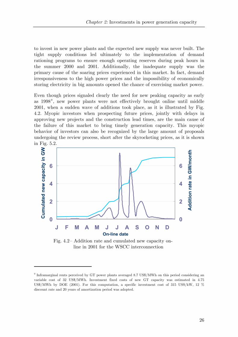
Chapter 2: Investments in power generation capacity
26
to invest in new power plants and the expected new supply was never built. The tight supply conditions led ultimately to the implementation of demand rationing programs to ensure enough operating reserves during peak hours in the summer 2000 and 2001. Additionally, the inadequate supply was the primary cause of the soaring prices experienced in this market. In fact, demand irresponsiveness to the high power prices and the impossibility of economically storing electricity in big amounts opened the chance of exercising market power.
Even though prices signaled clearly the need for new peaking capacity as early as 19989, new power plants were not effectively brought online until middle 2001, when a sudden wave of additions took place, as it is illustrated by Fig. 4.2. Myopic investors when prospecting future prices, jointly with delays in approving new projects and the construction lead times, are the main cause of the failure of this market to bring timely generation capacity. This myopic behavior of investors can also be recognized by the large amount of proposals undergoing the review process, short after the skyrocketing prices, as it is shown in Fig. 5.2.
9 Inframarginal rents perceived by GT power plants averaged 8.7 US$/MWh on this period considering an variable cost of 32 US$/MWh. Investment fixed costs of new GT capacity was estimated in 4.75 US$/MWh by DOE (2001). For this computation, a specific investment cost of 315 USS/kW, 12 % discount rate and 20 years of amortization period was adopted.
Fig. 4 .2 – Addition rate and cumulated new capacity on - line in 2001 for the WSCC interconnection
0
2
4
6
J F M A M J J A S O N D On-line date
Cum
ulat
ed n
ew c
apac
ity in
GW
0
2
4
6
Add
ition
rate
in G
W/m
onth

Chapter 2: Investments in power generation capacity
27
The high prices triggered a wave of massive investments in gas-fired power plants in the U.S. West Interconnections (WSCC) and in some other markets established in the southern U.S. As a result, overbuilding and excess of capacity have been observed in many regions. Particularly, the Texas Interconnection (ERCOT) has registered a sudden increase of the reserve margins, in excess of what would be reasonable for this market. Texas has been one of the first U.S. markets to bear overbuilding (EVA, 2003).
By the end of 2003, 192 GW of cumulated capacity since 1998 have been installed in the U.S. Additionally, almost 72 GW are planned to be brought online in period 2004-2007. In many U.S. regions, an overbuilding of generation capacity emerged (Hunt and Sioshansi, 2002). Debt ratings and financial positions of many merchant developers have deteriorated considerably. Under a near-inevitable bust cycle and industry downturn, many of them might suffer severe financial distress or even bankruptcy. Fig. 6.2 depicts the evolution of quotations at the NYSE of the four most important merchant developers in the U.S. markets. They reflect the high profitability expectations under the industry boom and the dramatic loss of firm value, as result of the expected erosion of firm earnings provoked by capacity overbuilding. In Fig. 7.2, the development of the reserve margin for the ERCOT interconnection, as well as the expected evolution at the aggregate national level is shown. From this figure, the
Fig. 5 .2 – Status of the new generating capacity for period 1996 - 2001
Source: Sweeney (2002)
0
2
4
6
8
10
12
14
1996 1997 1998 1999 2000 2001
Cap
acity
in G
W
CancelledUnder review Ready for constructionUnder construction New operational

Chapter 2: Investments in power generation capacity
28
fluctuating nature of the reserve margins, associated to a boom and bust cycle, can be easily recognized.
Fig. 6.2 – Evolution of stock prices of four important merchant developers during U.S. power industry downturn
0
20
40
60
80
1998 1999 2000 2001 2002 2003 2004 2005
Stoc
k Pr
ices
in U
S$
AESCalpineDynegyDuke
Fig. 7 - Development of the reserve margins for ERCOT and at the U.S. national level
Source: EIA, NERC, EVA(2002)
0
10
20
30
40
50
1994 1998 2002 2006 2010
Res
erve
Mar
gins
in %
ERCOTU.S.U.S. Forecast

Chapter 2: Investments in power generation capacity
29
Similarly what occurred in the U.S. markets, other power markets in the world have gone through some unexpected anomalies. Sharp decreasing of the reserve margin after the liberalization has also been observed in the Australian wholesale power market. As a consequence of the tight supply conditions in 2000 and 2001, high market prices prevailed during this period, as it is reflected in the monthly average spot prices, see Fig. 8.2. The entry of new power capacity relieves the situation, but that does not impede the high prices.
The capacity additions totalized 800 MW in the South Australian market, which represented an increase of 30 % with respect to the existing capacity. The result was a rapid decrease of peak prices eroding dramatically the profitability of peaking plants (IEA, 2003).
Similarly to the behavior observed in Australia, the Spanish wholesale market has evidenced a pronounced decreasing of the firm, dependable capacity. That is reflected in the tight reserve margin and the high peak prices during 2002, as it is illustrated in Fig. 9.2. A lot of generating projects, totalizing 38 GW based on CCGT and 22 GW based on wind have been announced or started (Alba, 2003). The Spanish generation system amounts 58.5 GW of installed capacity. As a result, considerable overcapacity conditions might emerge in this market, if all planned capacity is effectively brought online.
Fig. 8.2 – Development of the Australian power market alter liberalization Source: IEA (2002); KEMA (2005) and market data from NEMMCO

Chapter 2: Investments in power generation capacity
30
Oversupply as consequence of overbuilding has been also observed in the Argentinean power market. The high prices and the low reserve margins in Argentinean power system at the beginning of the restructuring in 1992 attracted a lot of foreign investors who triggered a wave of investments in CCGT-based merchant power plants. This rapid expansion led to high reserve margins (see Fig. 10.2 and 11.2) and a very competitive market. The excess of entries based on cheap generation lowered significantly the Argentinean wholesale prices during a prolonged period, which ultimately resulted in unprofitable investments. Indeed, investments have been stopped since 2001, though power demand has recovered rapidly after the macroeconomic crisis and power prices have escalated considerably.
Additionally, the over reliance on gas-fired technologies have endangered the long-term security of supply. Gas-fired capacity represents now 56 % of the installed capacity and approximately 40 % of the generation output (CAMMESA, 2002). Indeed, most of these power plants cannot be now accounted as firm capacity in winter, as there is not enough transport capacity in gas pipelines to fuel thermal power plants during peak hours. In winter 2004, many gas-fired power plants have switched to liquid fuels, what has been reflected in a considerable increase of wholesale prices, as it is depicted in Fig. 10.2.
Source: Alba (2003) and market data from OMEL
Fig . 9 – Development of the dependable reserve margin and power prices in the Spanish wholesale market after liberal i zation
0
10
20
30
1996 1998 2000 2002 2004
Res
erve
mar
gin
in %
0
40
80
120
Peak
Pric
es in
€/M
Wh Spain

Chapter 2: Investments in power generation capacity
31
Fig. 10.2 – Development of the reserve margin and power prices after restructuring of the Argentinean power market Source: CAMMESA
30
40
50
60
70
1992 1994 1996 1998 2000 2002 2004
Res
erve
Mar
gin
in %
0
25
50
75
100
Pow
er P
rices
AR
$/M
Wh
Argentina
25
Source: CAMMESA
0
5
10
15
20
1992 1994 1996 1998 2000 2002 2004
Inst
alle
d C
apac
ity in
GW
Diesel GT CCGT Steam Hydro Nuclear
Argentina
Fig. 11.2 – Evolution of the plant mix of the Argentinean generation system

Chapter 2: Investments in power generation capacity
32
In the former pool market established in UK, a similar behavior with a massive entry of new capacity based on CCGT technology, the so called “dash for gas” has also been observed. Currently, CCGT power plants have displaced large coal plants from the baseload supply. The relatively low operating costs, decreasing investment costs and short lead time for construction, have led to an addition of 22.5 GW of CCGT capacity being commissioned by 2002. Additionally, 29 GW are under review, though prices have declined sharply as result of overbuilding and entry costs of new capacity remain about 20-25 £/MWh. More than 10 GW of capacity, almost entirely oil and coal, have been decommissioned between 1995 and 2000.
Now, CCGT power plants account for one third of the installed capacity and approximately 40 % of the energy production. Between 1997 and 1999, the regulatory authority, concerned with the increasing dependence of the UK on gas-fired generation, imposed a moratorium on issuing additional licenses to construct CCGT power plants. Fig. 12.2 depicts the development of the reserve margin and the demand-weighted annual System Marginal Price (SMP) for the pool market established in England and Wales. Under regulated industry, expansion of the generating system was planned to maintain the reserve margin around the 25 % for meeting reliability requirements. Nevertheless, after liberalization the reserve margin has consistently remained below this figure.
Fig. 1 2 . 2 Develo pment of the former pool of England and Wales
–
0
5
10
15
20
25
30
1990 1992 1994 1996 1998 2000
Res
erve
Mar
gin
in %
15
20
25
30
35
Ann
ual A
vera
ge S
MP
in £
/MW
h
Reserve Margin
SMP
UK
Source: IEA (2002)

Chapter 2: Investments in power generation capacity
33
Other liberalized power markets around the world have faced electricity crisis caused by insufficient investments in expanding their generating capacity. A case is the power market in Alberta in 2001 and the recently reformed market in Ontario, which suffered from tight capacity and price spikes in 2002/2003. New Zealand also experienced energy shortfall in 2001 and 2003 because of a prolonged period of low hydro inflows. Though the market is well designed and it is functioning properly, the government has concluded that the current electricity market does not offer enough incentives to invest in peaking capacity (IEA, 2003).
Even Europe might experience a boom-bust cycle. The EU has liberalized their power markets enjoying of considerable overcapacity. Whilst peak demand was 415 GW in 2002, there were 700 GW of installed capacity with 550 GW accounting as firm capacity to meet peak demand. However, this excess of capacity is being rapidly decommissioned and mothballed, and it is expected to see a continuous net loss of capacity in Europe, as no relevant investment activity is expected to be observed in the next years. For this reason, power prices will rise in the future, with more frequent price spikes and lower reliability, configuring the boom period. However, a large amount of new capacity will be needed by 2012, facing Europe the first market test for attracting sufficient and timely investments. Most of this capacity will be based on CCGT technologies and renewables, with very low marginal cost of generation. Even without overbuilding, as occurred in UK, a boost in prices and investment returns is very likely (Jansen et al., 2003).

34
Chapter 3
Modeling power market dynamics
Power markets exhibit some structural characteristics, such as feedbacks and delays, which are determinant of the long-run behavior and cannot be easily captured by the traditional partial equilibrium models. In this chapter, an alternative modeling approach is developed, which is able to overcome limitations proper of optimization-based models.
After delimiting the technical and economic system under consideration in this thesis, the formal requirements for long-term modeling of electricity are stated. The basics of the selected mathematical framework for solving this problem are offered along with an overview of the developed market model. The model overview shows the relationship among the system components, and therefore, it will be useful for guiding the further discussions.
The long-term market model is divided in subsystems. In each section of this chapter, the subsystems are analyzed and a mathematical formulation in terms of the selected methodology is presented. The last part of the chapter offers a comprehensive perspective of the model by deriving the system’s state equations. The characterization of these equations is an essential part of the understanding of the long-run behavior of electricity markets.

Chapter 3: Modeling power market dynamics
35
3.1 System under study and general hypothesis
The industry model presented here can be characterized as a structural model (it might be also classified as a fundamental bottom-up model), since the long-run development of the power market is determined by modeling the variables having direct influence on long-term movements of supply and demand.
In this thesis, a simplified version of a thermal power system comprising three different plant technologies will be considered. Base (HC), middle (CCGT) and peaking capacity (GT) are characterized by their investment and operating costs. Investment decisions on each one of these technologies are determined endogenously by the proposed model. Fuel prices, the progress of thermal efficiencies of the various technologies, investment costs, and other important model parameters are however given to the model as exogenous variables. In Fig. 1.3, a view of boundaries of the technical system under consideration is offered.
Because of energy-only markets, with very few exceptions, dominate the scene in most countries, the developed market model do not account for capacity payments, though the model might be easily expanded to consider them. The model assumes that the standard two-settlement mechanism exists. i.e. all transactions are settled at prices prevailing in the real-time spot market, irrespective of commitments emerging of trades, which took place in any forward market. As most of the trade occurs in the energy market, ancillary services are not taken into account. In a majority of the systems, revenues
∼∼
Boundary of the technical system
HCCapacity
CCGT Capacity
GT Capacity
SystemDemand
Thermal Generation System
Endogenous variables
Exogenous variables
Mercado de Energía Wholesale
Power Market
• • • Investment costs •
• Fuel prices • Thermal efficiencies • • Interest rates • Demand growth
Investment decision
• Regulatory framework ∼
Boundary of the tecnical-economical system
Fig. 1.3 – Boundaries of the system under study

Chapter 3: Modeling power market dynamics
36
coming from ancillary services markets represent only a small fraction of generators’ revenue stream10.
In the price formation mechanism, perfect competition is assumed, i.e. agents behaving as price-takers and consequently bidding their true marginal costs. That is deemed to be a plausible assumption for markets with a low degree of concentration. Even if not, modeling power markets under a well-known economical framework is the first step towards understanding the basic mechanisms governing the system’s long-term behavior.
The developed model is focused on simulating system’s time response, instead of extracting closed-form analytical solutions. The time horizon for simulations has been set to 20 years, since most of the relevant dynamics of practical interest are revealed within this time frame.
3.2 Model requirements
A number of structural characteristics of the power generation industry have to be handled by the mathematical methodology selected for modeling the long-term evolution of power markets. The most prominent mathematical complexities to be considered are listed below:
Stochastic nature of many exogenous variables.
Non-linear relationships between variables.
Delays in some processes.
Informational feedback structures.
Additionally, the proposed model must consider various technical, economical aspects influencing the development of power systems, such as:
Generation costs of the existing generating plants, as well as the progress in the thermal efficiencies of new plants added further.
10 Some exceptions are systems with considerable wind generation, which imposes a higher demand on the different reserve and balancing markets. That might be the case of the German power system where high reserve prices are presently being observed. However, such prices might be the result of the low liquidity and low degree of competition registered in those markets.

Chapter 3: Modeling power market dynamics
37
Investment cost of generating technologies.
Construction lead-time for power plants of different technologies.
The typical long lifetime of generating facilities.
The probability of price spikes as consequence of generation shortages. For this purposes, the combined uncertainty on peak demand and plant availability have to be taken into account.
Patterns in electricity consumption over the year, as it determines the usage pattern of the various plant technologies.
Growth in peak and energy demand.
Regulatory framework, particularly price cap policies.
Investor delaying behavior upon uncertainties.
Expectation formations upon future conditions.
3.3 Mathematical framework
One of the most distinctive characteristic of economical agents is their forward-looking behavior, as they react primarily upon expectations and not upon the current system state. Thus, expectations among firms determine the system’s time path, and very likely the resulting time path will determine expectations (Evans and Honkapohja, 2001). This fact makes economical systems feedback-closed. Thus, the proposed mathematical methodology must contemplate the dynamic nature of the power markets. Mathematically, the future states of the system are a function of states that the system resided in the past:
1 1 2( , , ,..., )t t t t t ny f y y y y+ − − −= (1.3)
For this reason, it seems natural and straightforward to describe the power market with the usual tools developed to deal with dynamic systems. Economics has recognized the dynamic nature of most economical systems, but it has focused essentially on macroeconomic systems (Flaschel et al., 1997). Though separated from the economic mainstream, dynamicists have developed a self-contained discipline focused on microeconomic systems. They have oriented to the simulation of system behavior, instead of analyzing the analytical and

Chapter 3: Modeling power market dynamics
38
asymptotic properties of the dynamic equations. Under this approach, simplifications, such as linearizations, are not necessary and therefore the full dynamic equations can be considered.
The developed model in this thesis is based on such a discipline, known as System Dynamics (SD), which is a mathematical framework with the ability of suitably capturing complexities like those described in the previous section. SD is a branch of Control Engineering and System Theory applied predominantly to economical, business and managerial systems. The beginning of SD can be traced to the seminal works of Forrester in the late fifties (Forrester, 1961)11. A survey of applications of this methodology to the electricity industry can be found in Ford (1990).
This mathematical methodology is especially appropriate to handle dynamical systems at an aggregated level, since informational and physical feedbacks, non-linearities and stock and flows structures can be easily modeled. In general terms, the methodology of SD is based on identifying the structure of the system and the logic of the interrelationships among the different system components to derive its dynamical response. Mathematically, this results in the formulation of the differential state equations that represent the system behavior. Usually, given the complexity of real-world systems, it is only possible to solve these equations through numerical methods.
To represent such complex systems in an understandable manner, a specific set of analysis techniques and describing diagrams has been developed. In this section, and because they are used further throughout the thesis, a brief description of the notations of two important types of SD diagrams are given.
3.3.1 Causal Loop Diagrams (CLD)
CLD are an important tool for representing the feedback structure of systems. Long used in academic work and increasingly in business, CLDs are excellent for quickly capturing hypothesis about the causes of dynamics. CLDs are more flexible than block diagrams used in control engineering, which become unintelligible for large systems. Causal diagrams consist of variables connected
11 A complete and modern reference book on the SD methodology can be found in Sterman (2000).

Chapter 3: Modeling power market dynamics
39
by arrows denoting causal influence (named causal links) among variables. Each causal link is assigned a polarity, either positive (+) or negative (–) to indicate how dependent variable changes when independent variable changes. Important feedback loops can also be recognized in CLDs. Feedback loops are denoted as reinforcing (positive) or balancing (negative) and they are identified by a loop polarity sign.
Formal definitions are summarized as follows. Given a function Y dependent on n independent variables, the diagram:
can be mathematically expressed as:
1
0YX∂ >∂
or
0
01( ....) ( )t
t
Y X ds Y t= + +∫ in the case of accumulations.
On the contrary, the following relationship:
denotes:
1
0YX∂ <∂
or
0
01( ....) ( )t
t
Y X ds Y t= − + +∫ in the case of accumulations.
Additionally, the symbols in a closed loop denote the existence of a feedback structure: Positive (Reinforcing) feedback loop Negative (Balancing) feedback loop.
3.3.2 Stock & Flows Diagrams (SFD)
Even though CLDs are very useful, especially in the first stages of modeling, one of the most important limitations of causal diagrams is its inability to capture
X Y+1
X Y-1
+

Chapter 3: Modeling power market dynamics
40
explicitly the stock and flow structure of systems. Stocks and flows structures, along with feedback, are the two central concepts of dynamic system theory. Stocks are accumulations. They characterize the state variables of the system and generate information upon which decisions and action are based. Stocks create delays by accumulating the difference between the inflow to a process and its outflow. By decoupling rates of inflow from outflows, stocks are the source of disequilibrium in system dynamics. SFDs and CLDs can be also used combined to achieve a better description of system dynamics. Stocks are represented in diagrams under the following notation.
Mathematical formulations of stocks are given by the following expressions:
Integral form of stock equations
[ ] 0
0
( ) ( ) ( ) ( )t
t
Stock t Inflow s Outflow s ds Stock t= − +∫
Differential form of stock equations
( ( )) ( ) ( )d Stock t Inflow t Outflow tdt
= −
The contribution of stocks to system dynamics is essential and it can be summarized in the following points (Sterman, 2000):
Stock characterizes the state of the system. Many variables in systems depend on the current value of stocks.
Stocks provide systems with inertia and memory. Stocks accumulate past events. The content of a stock can only change through an inflow or outflow. Without changes in these flows, the past accumulation into stock persists over time.
Stocks are the source of delays. All delays involve stocks. A delay is a process whose output lags behind its input. The difference between the input and output accumulates into a stock. Perception delays, for instance, can be modeled as stocks though these stocks do not involve any material flow.
Stockoutflow rateinflow rate
source sink

Chapter 3: Modeling power market dynamics
41
Stocks decouple rate of flows and create disequilibrium dynamics. Stocks absorb the differences between inflows and outflows, thus permitting the inflows and outflows to a process to differ. In equilibrium, stocks remain unchanged. However inflows and outflows differ because they are governed by different decision process. Disequilibrium is the rule rather than the exceptions.
Real-world systems typically exhibit more than one stock and multiple interaction among variables is the rule. Variables changing very slowly in the considered time frame are modeled as constants. Variables that can change freely and hence are not subjected to interactions due to system dynamics are considered as exogenous variables. The derivatives of stocks in dynamic systems are, in general, non-linear functions of stocks, the exogenous variables, and some constants. In matrix notation, the rates of changes, d /dtS are a function f( ) of the state variables S, the exogenous variables U and the constants C,
( , , )d /dt f= =S S S U C (2.3)
Real systems are usually represented as a network of stock an flows connected by information feedbacks. Frequently, such systems contain hundreds of equations representing dynamical interactions. Actual system’s outcomes and time responses to inputs must always be simulated by numerically integrating the differential equations, since the practical impossibility of finding closed-form solutions by means of analytic techniques.
3.4 Model overview
Under the SD approach, the dynamics of power markets is described by a set of nonlinear differential equations that account for existing system feedbacks, delays, stock-and-flow structures and nonlinearities. A simplified causal-loop diagram of the power market is depicted in Fig. 2.3 to provide an overview of the system’s dynamical structure and to guide the further discussion when modeling the different system components. The diagram shows the basic balancing feedback that governs the long-run development of any power market. As long as the actual reserve margin12 becomes tight, the spot prices will rise because more expensive power plants will be scheduled. On the basis of current
12 Reserve margin refers here the capacity in excess of the peak load plus any capacity required for security considerations. In the present formulations, operating reserves are not accounted for.

Chapter 3: Modeling power market dynamics
42
market conditions and expected fuel prices, the market participants form expectations on future electricity prices. The expected prices play a crucial role as they determine the profitability of possible investment projects. The construction of new power plants will be decided only if there is enough certainty that the investment costs will be recovered. The first delay in the feedback loop is therefore regarding the investment irreversibility, i.e. the investment decision delay, which is denoted with 1τ . In addition to this delay, new power plants are required to get permissions and they need a certain time to be constructed and to be brought on-line. This second delay on the feedback loop is referred in the figure as 2τ . The existing capacity jointly with the additions of new capacity, the retirements of old power plants and the current system demand will determine the new reserve margin and the new prevailing price level. Thereby, the market turns self-balancing and resembles the negative feedback loops commonly encountered in control systems. This balancing
mechanism is responsible for maintaining an adequate reserve margin to ensure a reliable electricity supply.
Despite the usefulness of the presented CLD to represent the causal relationships and the market balancing feedbacks responsible of adjusting the production capacity, it is not capable to show explicitly stock-and-flow structures embedded in the system. In Fig. 3.3, the stock structure underlying delay 2τ is revealed. Important variables controlling rates of flows into stocks have been added, improving largely the understanding of the capacity adjustment mechanism.
Capacity
Reserve
Spot Prices
Expectations on Long-Term Prices
Expected Profitability
Investment Decision
+ -
+
+ +
+
Electricity Demand
Retirements
Expected Costs
-
-
-
Required Reserve Margin
+
Expected Price Fuels
1τ
2 τ +
Fig. 2.3 - Causal-loop diagram of the power market
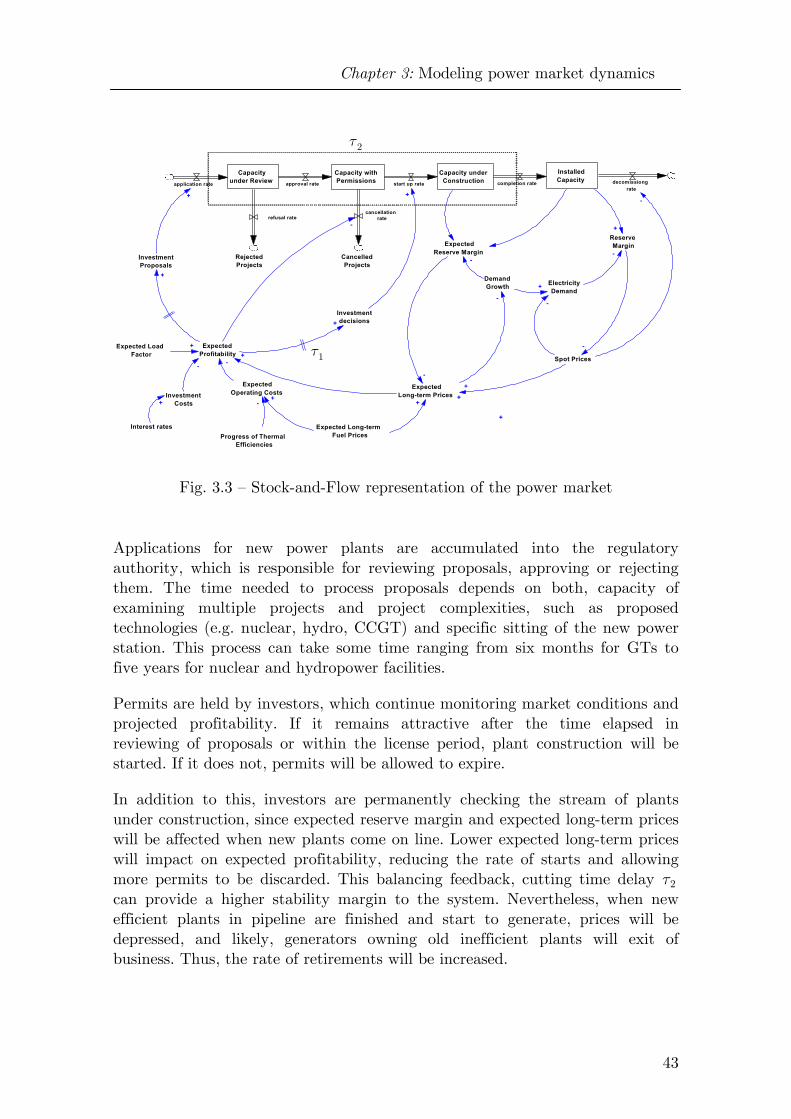
Chapter 3: Modeling power market dynamics
43
Applications for new power plants are accumulated into the regulatory authority, which is responsible for reviewing proposals, approving or rejecting them. The time needed to process proposals depends on both, capacity of examining multiple projects and project complexities, such as proposed technologies (e.g. nuclear, hydro, CCGT) and specific sitting of the new power station. This process can take some time ranging from six months for GTs to five years for nuclear and hydropower facilities.
Permits are held by investors, which continue monitoring market conditions and projected profitability. If it remains attractive after the time elapsed in reviewing of proposals or within the license period, plant construction will be started. If it does not, permits will be allowed to expire.
In addition to this, investors are permanently checking the stream of plants under construction, since expected reserve margin and expected long-term prices will be affected when new plants come on line. Lower expected long-term prices will impact on expected profitability, reducing the rate of starts and allowing more permits to be discarded. This balancing feedback, cutting time delay 2τ can provide a higher stability margin to the system. Nevertheless, when new efficient plants in pipeline are finished and start to generate, prices will be depressed, and likely, generators owning old inefficient plants will exit of business. Thus, the rate of retirements will be increased.
1τ
2τ
Capacity under Review Capacity with
PermissionsCapacity under
ConstructionInstalled Capacity
application rate approval rate start up rate completion rate decomissiong rate
Rejected Projects
refusal rate
CancelledProjects
cancellationrate
Reserve Margin Expected
Reserve Margin
Electricity Demand
DemandGrowth
Spot Prices
ExpectedLong-term Prices
Expected Profitability
Investment Proposals
Expected Long-termFuel Prices
Investment Costs
Progress of Thermal Efficiencies
Expected Load Factor
+
+
+
+
-
+
+
- -
-
-
Expected Operating Costs
+ - -
- ++
-
Interest rates +
--
Investmentdecisions+
+
Fig. 3.3 – Stock-and-Flow representation of the power market
+
+

Chapter 3: Modeling power market dynamics
44
Additionally to capacity decommissions, in this period electricity demand is expected to grow, and eventually reserve margin can become tight again, causing a new wave of constructions due to both, accumulated permits and a stream of new proposals. In the first case, starts are immediate; the second is delayed by the time needed to obtain permits. Hence, simultaneous decisions of investing in new plants will reach to the marketplace with different time-phase.
The stock-and-flow structure must be further expanded in parallel stock chains to take into account the different characteristics of the several available technologies. In fact, stocks representing the installed capacity, the capacity under construction, etc. have to be disaggregated to account for different lifetimes, construction lead-times, permitting delays, etc. Moreover, for a same generating technology, installed capacity has to be distinguished by age to keep track of thermal efficiencies, and therefore, the spread in marginal cost of production. In the following, a SD modeling approach for the different system components is developed.
3.5 Modeling the supply side
Long-run power market development is driven mainly by movements of the aggregate supply curve. In order to assess the influence of the different variables on the long-term dynamic behavior of power markets, a simplified generation sector, but with typical numeric values, has been modeled. A test system composed by a thermal generating park with three different generating technologies is considered: hard-coal power plants (HC), gas-fired combined cycles (CCGT) and gas turbines (GT). The initial system capacity amounts 16.4 GW including a reserve margin of 9 %, which was determined as economically optimal for this system as it is later shown in Section 3.8. From the total capacity 69.6 % corresponds to HC power plants, 22.5 % to CCGT technology, and finally 7.9 % to peak capacity based on GTs. These percentages represent the optimal technology mix, given the demand curve, and fixed and operating costs at the beginning of the considered time frame.
In order to determine endogenously the evolution of the supply curve as new capacity with higher thermal efficiency is added and old capacity is decommissioned, it is necessary to replicate the development of the age structure of the generating park. Thus, the capacity is differentiated for each technology in a number of vintages, vn . In the present model vn is limited to five. Vintage modeling and aging chains are usual in macroeconomic models where it is necessary to differentiate the capital by its productivity. In this case,
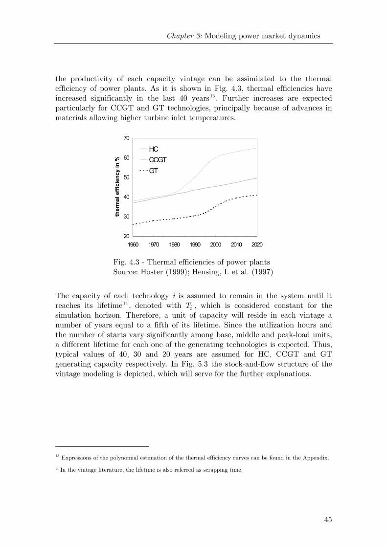
Chapter 3: Modeling power market dynamics
45
the productivity of each capacity vintage can be assimilated to the thermal efficiency of power plants. As it is shown in Fig. 4.3, thermal efficiencies have increased significantly in the last 40 years 13 . Further increases are expected particularly for CCGT and GT technologies, principally because of advances in materials allowing higher turbine inlet temperatures.
The capacity of each technology i is assumed to remain in the system until it reaches its lifetime14 , denoted with iT , which is considered constant for the simulation horizon. Therefore, a unit of capacity will reside in each vintage a number of years equal to a fifth of its lifetime. Since the utilization hours and the number of starts vary significantly among base, middle and peak-load units, a different lifetime for each one of the generating technologies is expected. Thus, typical values of 40, 30 and 20 years are assumed for HC, CCGT and GT generating capacity respectively. In Fig. 5.3 the stock-and-flow structure of the vintage modeling is depicted, which will serve for the further explanations.
13 Expressions of the polynomial estimation of the thermal efficiency curves can be found in the Appendix.
14 In the vintage literature, the lifetime is also referred as scrapping time.
20
30
40
50
60
70
1960 1970 1980 1990 2000 2010 2020
ther
mal
effi
cien
cy in
%
HCCCGTGT
Fig. 4.3 - Thermal efficiencies of power plants Source: Hoster (1999); Hensing, I. et al. (1997)

Chapter 3: Modeling power market dynamics
46
This type of vintage model is called putty-clay, since it is assumed once invested in a certain type of the power plant, the thermal efficiency will remain fixed until the plant is discarded15.
The capacity residing at each time t in a vintage j of technology i can be described through an accumulation resulting from the rate at which new capacity enters the vintage, and the rate at which old capacity abandons the vintage, denoted by ( )ij
inK t and ( )ijoutK t respectively. Mathematically, the
accumulation can be formulated as:
0( ) ( ( ) ( )) (0)
tin out
ij ij ij ijK t K K d Kτ τ τ= − +∫ (3.3)
where (0)ijK represents the initial capacity in the vintage at time 0t = . Recognizing that = −( ) ( / )ij ij
out inviK t K t T n 16 and that += 1( ) ( )ij ij
out inK t K t , the total generating capacity in the system at each time ( )TK t will be given by:
0
3
1 11
( ) ( ( ) ( )) (0)T Ti
tin in
ii ii
K t K K T d Kτ τ τ=
= − − +∑ ∫ (4.3)
Here, 1 ( )iniK t represents the rate at which power plants of technology i are
brought online, and − = 51 ( ) ( )in outi iiK t T K t is the retirement rate at which old power
15 This assumption seems plausible as adequate maintenance is routinely carried out on generating units to preserve their technical performance. In actual generation systems, this might be somewhat different because through repowering (sometimes called retrofit), power plants might later achieve a higher efficiency than originally projected.
16 This expression represents a pipeline delay. In pipeline delays, the outflow are related to the inflow by ( ) ( )outflow t inflow t T= − with T being the time delay. Pipeline delays are also known in the queuing
literature as FIFO delays (First-in First-out).
( )ijK t
( )outijK t
( )( )
ij
ij
K ttη
( )
( )
outijoutij
K t
tη
Fig. 5.3 - Stock-and-flow structure of the capacity vintage model
( )inijK t
( )
( )
inijinij
K t
tη

Chapter 3: Modeling power market dynamics
47
plants are being decommissioned. Analogously, the average thermal efficiency ( )ij tη for each capacity vintage j of technology i can be derived as:
0
( ) ( )1 1 1( ) ( ) (0)( )( )
ij ij
in outt
outinij ijij ijij
K t K tdt
t K t ttη ηηη
= − +
∫ (5.3)
where ( )ijin tη and ( )ij
out tη are respectively the thermal efficiencies of each capacity unit entering and leaving the vintage j at time t. It is worth to note that 1 ( )in
i tη and 5 ( )out
i tη will be the thermal efficiencies of capacity of technology i being installed and decommissioned at time t. For a given initial time, the initial average efficiency (0)ijη for each vintage j of technology i can be determined from the curves presented in Fig. 4.3 jointly with the age structure of the generating park at the initial time.
The average marginal cost of generation at each instant t for the capacity residing in vintage j, denoted as ( )ijMC t , can be now easily derived from the vintage average thermal efficiency ( )ij tη and the prevailing fuel prices ( )F
ip t at time t:
=( )
( )( )
Fiijij
p tMC t
tη (6.3)
In the simulations, fuel prices are assumed constant over the time horizon to avoid introducing exogenous source of dynamics. They are given as 6 €/MWh for hard coal and 10.5 €/MWh for natural gas. The model assumes constant specific investment costs over the whole simulation horizon, as we want to isolate the effect of endogenously generated market dynamics from those generated by external perturbations. This assumption seems currently very realistic, as most of conventional technologies can be considered mature and consequently show very small progress ratio. This is valid yet for CCGT technologies, which over the last 20 years showed a significant reduction in investment costs. Accordingly, most of the recent literature agrees that investment costs will remain in the current levels (measured in constant dollars) and no further reductions will take place in the future, see Colpier and Cornland (2002), Farmer (1999, 1997) and Hoster (1999).
The rate at which new capacity of technology i come to operation, 1 ( )iniK t ,
depends on the rate at which firms are investing. However, it does not depend on the current investment rate, but on the investment rate that prevailed at time = − C
it t T , with CiT denoting the average construction delay for technology
i. Fig. 6.3 represents the stock-and-flow structure for capacity additions of

Chapter 3: Modeling power market dynamics
48
technology i. Note that the whole vintage model described above is aggregated into the stock ( )TiK t . The state variable ( )C
TiK t represents at each time the total capacity under construction for generating technology i. This accumulation depends on the current investment rate ( )iI t in such a technology as well as on the total completion rate, = −1 ( ) ( )Cin
iiK t I t T .
The time of construction varies substantially among generating technologies. Previous works necessary to the plant erection, installation complexities and different grades of modularity and standardization are the main reasons for this variation in the construction delay. Even for the same technology, the construction lead-time can differ among projects as a consequence of the selected location, the size of the plant, the project-specific technology and other special requirements. Thus, different construction lags for a given technology are allowed by introducing a discrete distributed delay. Fig. 7.3 shows the construction time delays and their distribution for the different technologies as the fraction of capacity completion regarding the total rate of initiations. When modeling the construction lag as a discrete distributed delay, the capacity completion rate, 1 ( )in
iK t , must be expanded and it will be given by:
1 ( ) ( ) ( )C Cinii ik ik ik
kK t w T I t T= ⋅ −∑ (7.3)
where ikw are the lag weights representing the probability of exiting the delay at any time C
ikT and they must sum unity, i.e.:
( ) 1Cik ik
kw T =∑ (8.3)
CikT describes the time discretization, and in this context k is the number of
discretization steps of the delay distribution.
In the model, it is assumed that firms apply for permits with time in advance enough to build new plants, and therefore, they always hold enough permits to construct the desired amount of capacity. This can be a good assumption when, for example, long-established generating firms hold sites of decommissioned power plants to construct new ones. However, the assumption might not be
1 ( )iniK t 5 ( )out
iK t ( )C
TiK t ( )Ti
K t ( )iI t
Fig. 6.3 - Stock-and-flow structure of the construction delay

Chapter 3: Modeling power market dynamics
49
valid for some technologies, e.g. big hydro, coal and nuclear power plants, which might need much time to obtain the consent from many stakeholders. Additionally, in some countries, because of political and ecological issues, barriers to some generating technologies could cause at some time a shortage of permits. Similarly, during periods with a high rate of applications, such as in California short after the crisis, the authority responsible for reviewing proposals might see its capacity limited to process permits timely and cause a permit shortage. Nevertheless, a sudden wave of proposals is normally the consequence of low reserve margins and therefore low supply reliability conditions. In these cases, the authority aiming at relieving the situation would probably make rules more flexible (e.g. environmental assessments) to speed up the process of issuing approvals in order to avoid a permit shortage.
3.6 Modeling power demand
Since we are not interested in predicting short-term movements of electricity prices, such as those caused by weather, we can accept some loss of chronological information gaining in model simplicity. For this reason, the load is characterized by a Load Duration Curve (LDC), which results of sorting the chronological load from higher to lower. To avoid unnecessary complexity in the exemplary calculations a linear LDC with an initial peak load, (0)maxL , of 15 GW and a minimum load, (0)minL , of 10 GW at the start of the simulations is adopted. Furthermore, possible structural changes in the load pattern are neglected and the LDC conserves its linear pattern for the entire simulation period. Therefore, for 0t = , the LDC can be analytically expressed as:
fraction of the construction start
0
20
40
60
80
0 6 12 18 24 30 36months
Com
plet
ed c
onst
ruct
ion
in %
HC
CCGT
GT
Fig. 7.3 - Completed capacity as rate

Chapter 3: Modeling power market dynamics
50
( )(0) (0) (0) (0)max maxminL L L d L= − + (9.3)
where (0)L is the load level at the initial time exceeding a cumulated duration d , for a given initial maximum and minimum demand, (0)maxL and (0)minL respectively.
In addition, the economical demand for power is considered price-irresponsive in the short-term, which represents the observed inability of customers to adjust their electricity consumption at short notice17. Although the load is modeled as price inelastic, it is assumed that consumers will not be willing to purchase any power if the market price rises above the cost of being curtailed. This cost, denoted by VOLL, is generally set by regulators to contemplate the case when the market cannot be cleared because the available generating capacity is not enough to completely satisfy the price-irresponsive demand. For the base case simulation, the numerical value of VOLL is set to 1000 €/MWh.
A deterministic exogenous demand growth rate of 1 %/year was chosen for simulating the base case. Therefore, known the demand at the initial time, the load at any time t is given by the following expression:
( )(0) (0) (0) (0)M Mmg t g t g tmax maxminL L e L e d L e⋅ ⋅ ⋅= ⋅ − ⋅ + ⋅ (10.3)
with mg and Mg being the growth rate of the minimum and peak load respectively. For the case of a linear LCD, it can be demonstrated that if
M mg g g= = , the growth of the peak load is equal to the annual energy growth rate.
This growth rate has been increased by means of a ramp function in order to assess its influence on the long-run behavior of the power market. Rigorously, the growth of electricity demand is stochastic by nature. Indeed, temporary alterations of weather, transitory acceleration and downturns of the economic activity provoke random deviations of the growth rate around its long-run “normal” value. This value might be somehow related to the long-run economic growth as well as the population growth.
17 Electricity demand, if exposed to spot prices, might have some degree of responsiveness in a longer time frame by reallocating or reducing consumption. Changes in demand patterns might have some impact on the long-run development of power markets. However, long-run demand adjustments are not modeled since the lack of empirical evidence on the extent that this occurs. The investigation of price-driven long-run alteration in consumption patterns is beyond the scope of this thesis.

Chapter 3: Modeling power market dynamics
51
Therefore, a plausible and realistic way to describe the uncertain path of the demand growth rate is by means of a mean-reverting stochastic process18. A mean-reverting process is one that evolves fluctuating around a known mean. The simplest mean-reverting process, known as the arithmetic Ornstein-Uhlenbeck stochastic process, is the following:
( )dg g g dt dzη σ= − + (11.3)
Note that the expected change in growth rate dg after a time increment dt depends on the extent of the deviation from the long-run growth rate g and the speed of the reversion towards the mean, η . In Eq. (11.3), σ is the volatility parameter and z is a variable following a Wiener process, which is also called Brownian motion. It can be shown that the infinitesimal increment of the Wiener process dz, can be represented in continuous time by the following equation:
tdz dtε= (12.3)
where tε is a normally distributed random variable with mean zero and standard deviation of 1, i.e. (0,1)t Nε = . By writing Eq. (11.3) as a difference equation, Monte Carlo techniques can be applied in order to simulate multiple stochastic realization of the growth rate over the considered time horizon. In Chapter 4, stochastic simulations are performed on the system aiming at representing quantitatively the long-run market uncertainty originated in the demand growth rate and finding confidence intervals for the dynamic response. Details on the SD implementation of the Ornstein-Uhlenbeck stochastic process as well as on the estimation of numerical parameters of Eq.(11.3) are given in the Appendix.
3.7 Modeling electricity price formation
The electricity market is assumed perfectly competitive. Therefore, firms cannot strategically influence the market price, behaving solely as price-takers. In such a market setting, the price at each time equals the marginal cost of the most expensive running generator. The vintage model presented in Section 3.4 delivers the average marginal cost of generation at full output, ijMC , for each
18 Conceptually, a stochastic process is a variable that evolves over time, at least partially, in a random fashion.

Chapter 3: Modeling power market dynamics
52
capacity vintage j of technology i and for each time t. By sorting these marginal costs from the lowest to the highest, the dispatching merit order for the available generating capacity is determined. If now the ordered vintage marginal costs are plotted against the total cumulated generating capacity, the industry supply curve is obtained for each time. Jointly with the LDC, the supply curve allows to determine the simulated market price duration curve (PDC)19.
In a given period, the PDC function will specify the number of hours, during which a certain market price is equaled or exceeded. The methodology to simulate the market price formation is depicted schematically in Fig. 8.320. This price formation model, which accounts for the annual price distribution, allows us to derive the short-term inframarginal rent being perceived at each time by each generating technology and thereby, the market signals for the investment decision-making.
19 Like the LDC, the PDC can be assimilated to the complementary probability distribution function of power prices. By reversing the axis, the PDC can be written as ( ) ( : )D P D p P= ≥ denoting by p the price variable and P a particular value. From the distribution function, given by ( ) 1 ( )F P D P= − , the probability density function ( )f P can be obtained as the first derivative of ( )F P with respect to : ( ) ( )P f P D P′= − . 20 It is worth to note that the merit order is a simplified heuristic method to solve the unit commitment problem (UC), which assumes total operating flexibility for generating units. In fact, operating constraints of generating units influencing the optimal UC, such as startup costs, minimum downtime-uptime and minimum unit output are not considered.
1 D
€/MWh
D
MW
1 €/MWh D
LDC
PDC
Supply Curve
VOLL
Ddef
P
Fig. 8.3 - Price formation in a competitive power market by means of a supply curve and the LDC

Chapter 3: Modeling power market dynamics
53
Price spikes cover a substantial part of the plant fixed costs, and therefore, they play a crucial role in inducing investments (especially in peak-load power plants). Investors will hence evaluate the probability of occurrence and duration of these events. Therefore, the PDC must take into account the high prices paid during the infrequent price jumps. The sudden price spikes occur because of the response to tight supply conditions, such as unplanned outages of significant generating capacity during peak-load hours21. In this case, if the reserve capacity is enough, peak load will be served by more expensive units, which will set the price at a higher level. In case of insufficient reserve and absence of demand bidding activity, the load cannot be satisfied completely and the market cannot be cleared. Therefore, a price reflecting the resource scarcity must be administratively set.
3.8 Modeling price spikes
To take price spikes derived from generation deficits into consideration, a probabilistic reliability calculation relating the capacity reserve margin in the system and the expected duration of deficits was carried out and included in the proposed dynamic model. A two-state probabilistic generation model is built assuming identical units to allow the calculation of the outage probability table by means of the binomial distribution22. Therefore, an average unit size, avgP , and an unit forced outage rate (FOR) are assumed for all generating units. The outage probability table is calculated for different reserve margins and it has been limited to the first 20 entries since the probability of encountering more than 20 units on outage at any time turns negligible. To keep the model simple at this stage, generation capacity on maintenance is not taken into account in these computations.
This probabilistic generation model must be convolved23 with a load model to determine the risk of generation deficit as it is described by Billinton and Allan (1996). The load model is characterized by a set of seven LDCs to consider the
21 Tight supply conditions can also be a consequence of a loss of transmission capacity in important interconnections. This requires a jointly probabilistic treatment of the generation and transmission system.
22 A recursive technique based in convolving the probability distribution of the available capacity of each generating unit with the LDC or fast methods based on cumulants might be easily implemented to relax this assumption. For more details see Billinton and Allan (1996). 23 Convolution is the mathematical operation of summing two or more random variables.

Chapter 3: Modeling power market dynamics
54
load forecasting uncertainty. This discretization represents the different load class intervals whose occurrence probabilities are assumed to be normally distributed around its expected value. The standard deviation of the load forecast uncertainty, Lσ , is assumed constant and equal to 1%. Figure 9.3 depicts the procedure for determining the deficit duration for a certain capacity outage level kO , given a reserve margin and a determined load duration curve,
lLDC , of the load model. For each reserve margin resK , the expected deficit duration is given by:
7 20
1 1[ ( )] Pr( ) Pr( ) l
resdef l k kl k
E D K LDC O d= =
= ⋅ ⋅∑ ∑ (13.3)
where Pr( )lLDC is the probability of having the load within the class interval l, Pr( )kO is the probability of a capacity outage level kO , l
kd is the deficit duration for the considered lLDC , and the index k is in this context the number of generating units on outage. The probability of a capacity outage level kO is computed through the binomial distribution −=Pr( ) k k n k
nkO C p q with p FOR= , 1q p= − , n the total number of generating units in the system. Hence, the
outage level kO expressed in MW is ⋅ avgk P . The deficit duration lkd for each
reserve margin and lLDC can be computed as follows:
T
T
lmink
l lmaxmin T k
lmaxk
K O L
L K O L
K O L
− <
≤ − ≤
− >
(14.3)
1
0
Tlmaxl k
k l lmaxmin
K O Ld
L L
− −=
−
1
Duration
MW Installed Capacity TK
Reserve Margin resK
Available Capacity
Outage k O
lkd
lmin L
l max L
lLDC l k E
Fig. 9.1 - Deficit duration for a given reserve margin and LDC, when an outage kO happens

Chapter 3: Modeling power market dynamics
55
The reserve margin, either expressed in MW or referred to the peak load, is not an absolute measure of the system adequacy and therefore, some adjustments have to be made to consider different system and average unit size. Therefore, the probabilistic calculations must corrected for different unit average sizes, since the structure of the generating park is likely to change in the long-term as more flexible and smaller generation units are brought online and older big power plants (e.g. nuclear and coal) are decommissioned.
In Fig. 10.3, it can be observed that the expected deficit duration is negligible for high reserve levels and rises abruptly when capacity becomes tight. Two deficit duration curves are shown for different average unit sizes. It is noticeable that the average size of generating units plays an important role in the loss of load expectation, particularly in the range of reserve margins of 2.5-10 %. Therefore, the simulation model should provide dynamically the average unit size for the entire generating park as it evolves over time since the deficit duration expectations influence directly the investment outcomes, especially for peak-load power plants. For this purpose, typical capacity for added generating units: 300 MW, 200 MW and 50 MW for HC, CCGT and GT respectively is assumed. At start of simulations (0)avgP is 250 MW.
Furthermore, the probabilistic calculations of deficit durations must allow for an increasing system size, as the expansion in demand consumption can be substantial when considering a long time horizon. For example, peak demand growing steadily at a moderate rate, say 2 %/yr, will be almost 50 % higher after 20 years. Then, for a same reserve margin expressed as percentage of peak load and a same average plant size, higher peak load values imply more units on outage to result on a deficit situation. Therefore, for a larger system and all else
0
5
10
15
20
-2,5 0 2,5 5 7,5 10 12,5 15Reserve in %
Expe
cted
def
icit
dura
tion
in %
Lmax = 15000 MW Outage probability distribution: Binomial
FOR = 5% σL = 1%
Pavg = 500 MW
Pavg = 75 MW
Fig. 10.3 - Expected deficit duration vs. reserve margin

Chapter 3: Modeling power market dynamics
56
being equal, system probabilities of encountering the system without enough available capacity to meet load should be lower. That is reflected in Fig. 11.3, which illustrates the expected deficit duration for two different peak load values.
To take into account the influence of the system and unit size on the cumulated duration of price spikes a first-order Taylor expansion approach has been developed and integrated into the price spike model. In general, the expected deficit duration can be written as a function of the reserve margin, the average unit size and the peak load as:
( )E , ,avg maxdefD f R P L = (15.3)
The first-order Taylor expansion of Eq. (15.3) yields:
0 0 ( ) ( )E ( ) ( , , ) def def
avg avg maxdef def maxavg max
D R D RD R D R P L P L
P L
∂ ∂ = + ∆ + ∆ ∂ ∂ (16.3)
The first term delivers the function at the initial system conditions. The latter two terms adjust the function to deviations occurred over time in the average unit size and peak load with respect to the initial conditions. The partial derivatives have been computed for different reserve margins. Fig. 12.3 illustrates as example the behavior of the partial derivatives with respect to the average unit size for the test system under study.
0
5
10
15
20
-2.5 0 2.5 5 7.5 10 12.5 15Reserve Margin in %
Expe
cted
def
ict d
urat
ion
in % Peak Load 10 GW
Peak Load 30 GW
Fig. 11.3 – Expected deficit duration for different system sizes

Chapter 3: Modeling power market dynamics
57
With these functions, the optimal level of supply reliability for the system might be determined. This occurs when the cost of serving an additional MW of peak load equals the cost of installing and operating an additional MW of peak capacity. From this condition, given VOLL and the investment cost of a unit of peak capacity, the economically optimal expected duration of load curtailments can be determined as it was done in Eq. (5.2) for 3D . For a given average unit size, the optimal reserve margin is easily derived from the curves of Fig. 10.3 and corrected for system size with Eq. (16.3).
Finally, the normalized expected price spikes revenues to be perceived by online generators can be calculated as a fraction q of the expected deficits duration, E[ ]defD , times VOLL:
( ) = ⋅ ⋅ ( ) E ( ), ( ), ( )avg maxdef defR t D R t P t L t q VOLL (17.3)
3.9 Modeling investor’s behavior
The underlying hypothesis in the discussion of this section is that investments in generation capacity are only driven by their economical attractiveness at each time. At the industry level, the attractiveness of investing in a certain generation technology at time t is assumed to be well described by its economic profitability expectation.
0.E+00
2.E-05
4.E-05
6.E-05
8.E-05
1.E-04
-2.5 0 2.5 5 7.5 10 12.5 15Reserve in %
Part
ial D
eriv
ativ
e
Fig. 12.3 – avgdefD P∂ ∂ vs. reserve margin

Chapter 3: Modeling power market dynamics
58
The model must consequently consider the manner that firms process the available information to form their expectations on future price distribution, and thereby on future profits. Therefore, some hypothesis about the expectation formation among firms on future market conditions has to be made.
3.9.1 Expectational hypotheses: REH vs. BRH
Historically, economics has used different approaches to represent expectations of economical agents, ranging from static and naïve expectations to adaptive, extrapolative and regressive expectations. To derive the aggregated expectation formation among investors, currently economics offers two essentially different approaches. Since the publication of the seminal article of Muth (1961) the rational expectation hypothesis (REH) is the prevailing approach in the neo-classical economic literature. Under REH, it is assumed an optimal forecasting behavior and hence investors are considered intertemporal optimizers when they made forecasts. This implies the rejection of the temporal causality hypothesis, i.e. expectations on future system states do not depend on past states. It is assumed that firms hold a very complete knowledge of the structural equations and parameters describing the system that they are trying to forecast, and thus, the possibility of systematic errors in the forecasting behavior is ruled out. In general, this might not be the case when objective probabilities of relevant variables cannot be evaluated such as when firms face strategic or behavioral uncertainties, i.e. uncertainties in determining a priori the action of other competitors.
The REH is presented in two forms. The strong form of the REH is usually known as perfect foresight. Agents’ forecasts made at time t for the value of some variable X at a future time T coincide with the realized value of the variable. Under perfect foresight, expectations are equated to actual outcomes. Mathematically, that is:
( , ) ( )e t T Tχ χ= (18.3)
Although this assumption is frequently convenient for the mathematical treatment of many economical problems, and for this reason widespread among modelers, economists recognize its very restrictive nature. Indeed, actual forecasts are almost always inaccurate. For this reason, the weak form of the REH assumes forecasting errors, though non-systematic:
( , ) ( )e t T Tχ χ ε= + (19.3)

Chapter 3: Modeling power market dynamics
59
where ε is a serially and mutually uncorrelated finite-variance term with a mean of 0.
Though useful as benchmark, the REH is usually rejected in econometric investigations testing for rational expectations in real-world economic systems24. In agreement with this empirical evidence, the second approach for modeling aggregate expectation formation is the bounded rationality hypothesis (BRH). It is based on the fact that firms do not know the exact specification of the system they are trying to forecast, and therefore, the structure of forecasting models and many model parameters must often be judgmentally estimated. Frequently, experience of forecasters is claimed as being a crucial part of the forecast process and essential for consistency of outcomes. This fact allows modelers enough freedom to adjust their forecasting models until they deliver results in reasonable agreement with the conventional wisdom prevailing at that time. As past and current values act as an anchor for conventional wisdom, adaptive expectation formulations based on exponential smoothing of past values and trend extrapolation can well replicate aggregate forecasting behavior25. While firms forming always their expectations in a full rational manner would be desirable, we must however model the actual forecasting behavior to derive the system’s dynamical response.
3.9.2 Modeling expectation formations under BRH
Any plausible expectational model must take into account, two main factors. Expectations are always subjected to revisions and reconsiderations upon observed changes, and they are formed only on observable, available information.
24 See for example the numerous empirical studies cited by Conlisk (1996) rejecting the RE behavior in a wide range of systems. Furthermore, in the context of electricity markets, first studies about the informational efficiency of futures markets reject the rationality hypothesis (Gulay Avsar and Goss, 2001) and offer some evidence that the future prices are driven by past levels of spot prices (Poskitt and Tomlinson)
25 Other strong argument against the REH underlies itself in the assumption of optimizing behavior of economical agents. The REH requires a great deal of knowledge of the system being forecasted, but probably firms prefer imperfect, incomplete models. Indeed, firms have the choice of using simple models and rule of thumbs at no cost or sophisticated models at very high costs. Complex modeling, information and data gathering usually are expensive. The optimal choice of the forecasting model is frequently something in between.

Chapter 3: Modeling power market dynamics
60
The first BRH approach is based on adaptive expectations, which have been widely used in macroeconomics. Under this framework, current expectations are related to current and past values in a distributed lag fashion. In discrete time, adaptive expectations can be written as:
( , ) ( , 1) ( 1) ( , 1)e e et T t T T t Tχ χ λ χ χ = − + − − − (20.3)
In other words, expectations on the value of the variable for time T are revised if the value forecasted in the previous period is different from the actual realization of this variable. The parameter λ ranges in interval [ ]0,1 and it is the rate of adjustment of expectations as a fraction of the forecasting error in the previous time interval. Note that if 0λ = , agents are myopic and do not revise their expectations under any circumstances, leading to static expectations. If 1λ = , the expectations are automatically linked to the last realized value, i.e. naïve expectations. The problem of firm holding adaptive expectations is that their expectations can be consistently wrong, in particular when agents are forecasting growing processes, as a forecast steady state error remains.
By acknowledging that such a forecasting behavior seems seemingly implausible as there are more efficient forecasting rules readily available, Sterman (1987, 1988) proposed a more refined expectational model based on SD. He recognizes that expectations respond not only to recent and past values, but also to change rates. His TREND function represents a comprehensive behavioral theory of how agents form expectations accounting for the time needed to measure, collect and analyze data, the historic time horizon they use, and the time required to perceive and react to variable changes.
The causal structure of the trend function is shown in Fig. 13.3

Chapter 3: Modeling power market dynamics
61
The TREND function delivers the expectation on the long-term fractional rate of change of a fluctuating input variable. It contains three informational stocks representing first-order exponential smoothing processes, which require of three parameters (the adjusting time constants), i.e. TPPC, THRC and TPT26.
The time to perceive the current state (TPPC) arises from the time needed for gathering data. For example, data on the annual peak load or the installed generating capacity is reported quarterly or even yearly. TPPC should be not lower than measurement lags. Decision makers compare the perceived present condition (PPC) to the last known state of the variable, i.e. the reference condition (RC) in order to determine if an upward or downward movement exists. The reference condition adapts progressively to new available information. The THRC determines how fast the reference condition is adjusted
26 For the underlying mathematical formulation of the first-order delays embedded in the TREND function see Sterman (2000).
PPC = Perceived Present Condition RC = Reference Condition of the Input PGR = Perceived Growth Rate TPPC = Time to Perceive the Present Condition THRC = Time Horizon for the Reference ConditionTPT = Time to Perceive the Trend ITREND = Indicated Trend
PPC
RC
PGRchange in PPC
change in RC
changein PT
THRC ITREND
TPPC TPT
Last observed value (INPUT)
Expected fractionalgrowth rate (OUTPUT)
Fig. 13.3 – SFD of the TREND function (Sterman, 2000)

Chapter 3: Modeling power market dynamics
62
and which is the relevant historical horizon for the reference condition. By comparing the PPC with the RC, the perceived change can be recognized. Nevertheless, a change in the perceived trend is not readily accepted as a sustained alteration of the trend. In fact, beliefs are not instantly adjusted to the most up-to date information. This lag is represented by TPT.
The expectation on the value will take a variable in a future time T, given its past development can then computed as (Sterman, 2000):
[ ] ( )( )( , ) ( ) 1 ( ) PGR t T te t T PPC t TPPC PGR t eχ −= + ⋅ (21.3)
Sterman (1987, 1988, 2000) shows that expectations on many important economic variables can be explained and well replicated by considering only backward-looking rules, what of course is inconsistent with the rational behavior. Energy demand and inflation are two examples of variables, in which much forecasting effort is spent and whose expectation formations can be reasonably well replicated by exponential smoothing and trend extrapolation. The fact that these two variables are periodically forecast using very sophisticated models suggests that even when agents face repeated opportunities to improve their forecasts, they might see their learning capacities limited in complex systems. That is particularly true when information and new evidence arrive at very slow rates. Thus, against what is often argued, the convergence to the RE behavior by learning might be very slow or unwarranted at all.
Therefore, a bounded rationality approach by means of the TREND functions is implemented to model the expectation formation on the future development of electricity demand, installed capacity and price distributions.
3.9.3 Profitability of power plant investments
By neglecting non-fuel costs and operational constraints, the present value of the cumulated operating profits that a proposed MW of generating technology i,
( )iT tπ , would realize over the amortization period aT , if the construction were to be actually started at time t, is given by the following expression:
+−= − ∀ ≥∫( ) [ ( ) ( )] ( ) ( )
T
t To ai i i
tot q e p MC d p MCρτπ τ τ τ τ τ (22.3)
where q is the availability of the generating units, ( )p t is the future development of power prices, ( )iMC t the marginal generation cost, which will depend upon

Chapter 3: Modeling power market dynamics
63
the fuel price development and the thermal efficiency of the proposed plant. = +0
Cit t T is the time at which the plant would be brought online if it were to be
effectively constructed, and ρ designates the risk-adjusted discount rate used to calculate the present value of future revenues. A price development and a marginal generation cost over time for technology i are depicted schematically in Fig. 14.3.
The cumulated operating profit [€/MW] over the amortization period is represented as the shaded area delimited by the marginal cost curve and the power price curve. Eq. (22.3) can be well approximated by summing the present value of the annual operating profits, ( )ik tπ , for the entire amortization period:
( )
1( ) ( ) (1 ) 1,2,...,
a Ci
T k
Tk T
ai ik
t t k Tπ π ρ − +
=≅ ⋅ + =∑ (23.3)
with ( )ik tπ measured in [€/MW·yr] and expressed as:
1( ) [ ( ) ( )] ( ) ( )
t ko
k kk t koi ii k kt q p MC d p t MC tπ τ τ τ
+
+ −= − ∀ ≥∫ (24.3)
where kiMC is the average marginal cost for the period k determined by the annual average fuel price, ( )F
ip t , and the thermal efficiency of the proposed plant. For each year k, the power prices can be accurately represented by an annual PDC, which contains the full information on the annual price distribution. Since forecast long-term power and fuel prices are subjected to high uncertainties, it is unlikely that investors know the true PDC of power and fuel prices for each future annual period k. It seems logical therefore to represent
time
€/MWh
0Cit t T= + 0 at T+
( )p t
( )iMC t
Fig. 14.3 - Cumulated operating profits for a MW of technology i over the amortization period

Chapter 3: Modeling power market dynamics
64
the aggregated investor’s expectations on future power prices formed at time t in terms of an expected price distribution, ( )ePDC t , for the entire period. From this curve, expectations on the present value of cumulated operating profits will be given by:
( )
1( ) ( ) (1 )
a Ci
T
Te e k Ti i
kt tπ π ρ − +
== +∑ (25.3)
with ( )ei tπ measured in [€/MW·yr] and expressed as:
0( ) [ ( ) ( )]
di ee eii t q PDC t MC t dDπ = −∫ (26.3)
where eiMC is the expected average marginal cost of generation, which depends
upon expectations on average fuel prices for the entire period and the state-of-the-art thermal efficiency available at time t. Indeed, neglecting operational constraints, power plants will be dispatched each time the prevailing price exceeds their generation marginal costs. Then di in [h] is the cumulated time this technology was operated in a year. Therefore, the expectations formed at time t on the operating profits that a MW of new capacity of technology i would make on the power market can be determined from the enclosed area between the expected PDC and the expected average marginal cost for such a technology, as it is shown in Fig. 15.3.
8760
Duration
€/MWh
id
eiMC
( )ei tπ
( )ePDC t
VOLL
Fig. 15.3 - Derivation of the expected operating profit from the expected PDC
E defD

Chapter 3: Modeling power market dynamics
65
The ePDC shown in Fig. 15.3 includes the expected price spike duration given by Eq. 17.3. Under the BRH behavior, expected price spikes durations are predicted by smoothing recent data of relevant variables and projecting recent trends for load growth, installed capacity, reserve margins and average plant size. For this purpose, the TREND function based on adaptive expectations as proposed by Sterman (2000) is implemented. Similarly, this TREND function is applied to construct the rest of the PDCe based on current and past values of the price distribution. The parameters of the TREND function are set as follows: TPPC=12 [months], THRC=60 [months] and TPT=36 [months] 27 . These parameter values are in close agreement with those found by Sterman for long-term energy forecasts. Additionally, the forecasting horizons are different for the various technologies: 10, 5 and 3 years for HC, CCGT and GT technologies respectively.
The economic profit expectation formed at time t, ( )eTi tΠ in [€/MW], for one
MW of capacity of technology i results from comparing the present value of the expected stream of operating profits with the investment cost that would be incurred at time t to install an unit of capacity of technology i, ( )iIC t . Mathematically, it is given by the following expression:
− +
== − = + −∑ ( )
1( ) ( ) ( ) ( ) (1 ) ( )
a Ci
T Ti i
Te e e k T
i i ik
t t IC t t IC tπ π ρΠ (27.3)
Acknowledging that the summation of the discount factors can be simplified as:
1
1(1 ) [1 (1 ) ]
aa
Tk T
kρ ρ
ρ− −
=+ = − +∑ (28.3)
and dividing both sides of Eq. (27.3) by the right side of Eq. (28.3), we obtain the economic profit expectation expressed as an annuity [€/MW·yr]:
−−
⋅= ⋅ + −
− +
( )( ) ( ) (1 )
1 (1 )Ci
a
e e T ii i T
IC tt t
ρπ ρ
ρΠ (29.3)
The second term on the right hand of Eq. (29.3) is the investment fixed expressed in [€/MW·yr]. If both sides of Eq. (29.3) are normalized dividing by the total hours in a year, the hourly average expected economic profit for investments in technology i is obtained:
27 See Sterman (2000), pp. 658-659, to initialize the TREND function.

Chapter 3: Modeling power market dynamics
66
−⋅ +
= −( ) (1 )
( ) ( )8760
Cie T
e ii i
tt FC t
π ρΠ [€/MWh] (30.3)
To be undertaken, investment proposals must normally exceed a corporate hurdle rate, which represents the long-term corporate opportunity cost of capital. For this reason, a suitable measure of project profitability is the internal rate of return (IRR), as it is widely used in corporate investment appraisal. The IRR can be computed from Eq. (29.3), as the discount rate, 0 ( )i tρ , at which the present value of the operating profits (the inflows) equals the investment costs (the outflow), and therefore, the expected economic profit delivered by the investment project is zero:
−−
⋅ = ⋅ + − =
− +
0 ( )1( ) ( ) (1 ) 0
8760 1 (1 )
Ci
a
e e o T i ii i i o T
i
IC tt t
ρπ ρ
ρΠ (31.3)
The advantage of the IRR [dimensionless] in this context is that the profitability can be expressed by a single number, independent of the project size and the individual corporate discount rate. Therefore, it is suitable to be compared with the industry-wide hurdle rate28. For the computation of 0 ( )i tρ in Eq. (31.3), constant values, currently typical for the specific investment costs are assumed: 1000 €/kW, 600 €/kW and 300 €/kW for HC, CCGT and GT technologies respectively. Amortization periods of 25, 20 and 15 years for HC, CCGT and GT investment projects are considered as well.
The econometric test presented in (Anderson and Goldsmith, 1997) shows that expectations on future profitability have a significant explaining power of the aggregate sectorial investments in a wide range of liberalized industries. Here, it is hypothesized therefore that the investment rate in each generating technology accelerates when firms hold expectations of supernormal profits, i.e. profitability above the opportunity cost of capital, and conversely, decelerates if profitability expectations indicate subnormal profit, i.e. profitability falling under the average industry-wide hurdle rate. However, in perfectly competitive markets even with moderate amounts of uncertainties, irreversible investments are committed only when expected returns exceed the opportunity cost of capital by
28 A drawback of the IRR-method is that a closed-form solution cannot be found and it can be only solved numerically. Other criticism is the underlying assumption that firms have the opportunity to reinvest the project cash-flows at the project IRR. In most cases, a better reinvestment assumption is the corporate opportunity cost of capital, i.e. the discount factor ρ. To overcome this problem, a modified IRR (MIRR) has been proposed. Nevertheless, we keep the IRR-method as most firms continue to use it for their investment appraisals.

Chapter 3: Modeling power market dynamics
67
a significant margin (Dixit and Pindyck, 1994). The classical investment threshold given by the NPV-method no longer applies, since the value of the project must not only outweigh the project direct costs, but also the opportunity cost of exercising the investment option. This fact provokes a delay in the investment decision with respect to the time point at which investment decisions would be made in an uncertainty-free environment. This behavior is explained by the value of the option to postpone irreversible investments facing uncertainties until more information (though never complete) about the future arrives. The optimal investment delay can then be determined when the marginal value of an additional bit of arriving information equals the forgone profits.
Other source of inertia in corporate investment decisions is that internally approved corporate investment plans are not generally modified with every bit of new information, since that would disturb the implementation of the corporate strategy whose stability is regarded as extremely important (Bromiley, 1986)29.
In the simulation model, an investment decision lag is implemented by delaying the IRR by a constant amount, inv
iT depending on the generating technology considered. The value of the delay depends on the uncertainty involved in projects of each technology. Generation technologies with a high ratio of investment costs to operating costs are more likely to suffer longer delays under uncertain future conditions. The investment decision is driven by a delayed IRR-signal during upward movements of the profitability expectation. However, the decision of investing at a lower rate during downward movements will follow the non-delayed IRR signal. The rationale behind this assumption is that once the value of the postponement option is zero (the profitability threshold is exceeded), the NPV rule applies directly and therefore the investment decision delay approaches zero. We assume that projects will be not delayed after aggregate profitability expectations reaching the maximal value, since the investment threshold is assumed to be always surpassed. Consequently, no delay is applied when the market is lowering its profitability expectations. If an investment decision delay were to be applied during the downward movements of profitability expectations, investment rates will remain much higher than the correct level when expectations indicate negative profit for new investments.
29 Commonly, firms’ investment strategies are revised on a yearly basis and 6 month are required approximately to prepare a new investment plan.

Chapter 3: Modeling power market dynamics
68
The driving investment signal at each time is given therefore by −0[ ( ), ( )]o inv
i i imin t t Tρ ρ .
A profitability index, PI, for each generating technology i is defined as the ratio resulting from dividing the driving IRR signal for such a technology evaluated at time t by the average required rate of return at the industry level, RRR:
−=
0 0[ ( ), ( )]( )
( )
invi i i
imin t t T
PI tRRR t
ρ ρ (32.3)
3.9.4 Modeling aggregate investment rates
In a competitive market remaining on the long-term equilibrium, the profitability index for each technology is 1iPI = since the IRR equals the prevailing average RRR at that time. As it was discussed in Section 2.5, under these circumstances the market does not offer any incentive for new entries or exits. Exits of old power plants being decommissioned will therefore be replaced by the entry of new ones, which will cover the retired capacity and the long-term perceived demand growth30. By this balancing mechanism, the long-run equilibrium is always attained. Thus, under zero economic profit the investment rate in technology i, ( )iI t , will be described by the decommissioning rate of generating capacity of the considered technology, 5 ( )out
iK t , and the capacity addition rate necessary to cover the expected growth of the maximum load served by this technology, ( )iL t :
11
5( ) ( ) ( ) ( ) ( )ref
PIPI
outi i i i iI t I t I t K t L t
t ==
∂= = = +
∂ (33.3)
Assuming that peak demand and the minimum demand are expected to grow at the same constant annual rate g, the maximal and minimum load at any time follow:
( ) (0)
( ) (0)
gtmax max
gtmin min
L t L e
L t L e
= ⋅
= ⋅ (34.3)
30 In growing industries, growth trends tend to be incorporated in firms’ capacity expansion planning, otherwise firms would systematically hold insufficient capacity to satisfy the growing demand. The power sector is considered still a growing industry as in most of the countries demand for electricity has been continuously growing since its widespread use was possible.

Chapter 3: Modeling power market dynamics
69
Under long-run equilibrium market conditions, the maximal load economically served by technology i at time t can simply be derived from the linear screening curves and the LDC prevailing at that time. The optimal capacities for each technology, denoted by *( )iK t can be determined by assuming that the LDC conserves its linear pattern over the simulation horizon and considering the optimal durations determined by Eq. (5.2):
*1 1*2 2 1*3 3 2
( ) [ ( ) ( )] ( )
( ) [ ( ) ( )] ( )
( ) [ ( ) ( )] ( )
max maxmin
maxmin
maxmin
K t L t L t D L t
K t L t L t D D
K t L t L t D D
= − +
= − −
= − −
(35.3)
By introducing Eq. (34.3) into Eq. (35.3), and by differentiating the latter with respect to time, the addition rate of capacity for each technology, = ∂ ∂*( )i iL t K t , required to optimally cover the growing demand can be obtained to be substituted in Eq. (33.3).
As power markets might expectedly deviate from the long-run equilibrium, the profitability expectations for some technologies at some times can significantly differ from the prevailing industry-wide average RRR. If profitability expectations for some time are above the average capital opportunity cost and assuming no barriers for new entries, it will be expected that aggregate investment rate for such technology exceeds the reference investment rate for the equilibrium case, i.e. ( )ref
iI t . Indeed, as long as PI for some technology increases, more investment projects based on such generating technology will become profitable, even for projects riskier than average or for companies facing higher firm–specific risks, and thus, with higher costs of accessing the capital markets. The extent to which the investment rate increases with the perceived profitability depends upon how much information on competitors’ investment plans is disclosed and the number of market participants following the actions of the leading firms, i.e. herding behavior. For a somewhat high profitability level, it seems logical that investment responsiveness shows a saturation level since participants are aware of the high attractiveness for investing and the potential danger of a wave of massive entries. Furthermore, in concentrated markets, a market participant holding significant market share might limit its own investments, since it would endanger the profitability of its own capacity in place. Another factor limiting the investment rate at high profitability levels are financing constraints to fund simultaneously many investment projects, as firms

Chapter 3: Modeling power market dynamics
70
normally must hold an equilibrated debt to equity ratio31. On the other hand, when the aggregated perceived profitability falls under the average opportunity capital cost, fewer projects will be profitable and only firms with lower capital costs will be willing to invest32. In this case, the aggregate investment rate will therefore be under the reference level.
According to this reasoning, a proposed nonlinear functional form for the investment responsiveness to the profitability level is depicted in Fig. 16.3. On the y-axis of the figure, the multiplier im for the reference investment rate is described as a function of the profitability index PI. It would be desirable to estimate the exact form of these curves when modeling an actual power market33. At the knowledge of the author, such investigation for conventional generating technologies remains undone. Nevertheless, the plausibility of the assumption is confirmed by the results presented by Morthorst (1999), which show that investment responsiveness to the expected profitability of private-owned wind turbines in Denmark are nicely fitted with a S-shaped curve.
31 An additional factor contributing for an upper limit in capacity additions is the limited delivery capacity of manufacturers to satisfy immediately the demand for new power plants when a construction boom in a big market occurs. 32 As business strategies and expectations are non homogenous among firms and even some firms can be misestimating future profit potentials, we can expect also to find some firms willing to invest even though the generalized belief in the industry indicates non-profitability conditions for new investments.
Aggregate investment responsiveness to the profita bility index
Con
stru
ctio
n St
art R
ate
0
1
2
3
-1 0 1 2 3 4 Profitability Index (PI)
Effe
ctt o
n th
e
Investments HCInvestments CCGTInvestments GT
Fig. 16.3 -

Chapter 3: Modeling power market dynamics
71
A logistic function has been used to describe the investment multiplier im for each generation technology:
( )1
maxi
i PI
mm
e α β− ⋅ +=
+ (36.3)
where maxim is the saturation level, α controls the slope of the sigmoid and β
determines its location with respect to the x-axis. The curves have been adjusted to satisfy the following condition:
11
PIim i== ∀ (37.3)
The investment rate at time t in generation technology i will therefore be computed as:
( ) ( ( )) ( )refi i iI t m PI t I t= ⋅ (38.3)
A different saturation level maxim has been hypothesized for each generating
technology. The saturation level for HC power plants is set relatively low, as it is unlikely that a severe investment over-reaction in this type of plants happens:
As base-load power plants (e.g. nuclear, coal, lignite and hydro) have to undergo normally long permitting processes before being constructed, information about investment plans considering these technologies are known by competitors well time in advance. Then, a competitor holding plans to construct a base-load power plant can cancel it before starting the construction.
Additionally, because of the plant size, such investments are typically made by well-established and experienced firms, which hold a good knowledge of the possible actions of competitors. The possibility of “herding behavior” is therefore greatly diminished.
Because of the typical huge size of base-load power plants, a very small number of competitors overreacting can cause significant overcapacity. This
33 Since power markets are relatively new, there are not enough data for a particular market covering periods with high profitability as well as times of low returns. For estimation purposes, data of several markets having experienced different profitability conditions might be normalized and aggregated to estimate an investment responsiveness function.

Chapter 3: Modeling power market dynamics
72
factor contributes to limit the responsiveness of each firm upon high profitability levels.
In addition, given the massive capital expenditures required for base-load plants, only few market participants are able to undertake such investments. As a consequence of the long construction time of these plants, even big firms might not undertake a second base load power plant project for an extended period of time.
On the contrary, the saturation level for CCGT power plants is set relatively high, since a high degree of responsiveness of the investments in this technology upon the profitability level has been observed in actual markets. Some reasons for this behavior are:
Because of the plant size and the environmental advantages, proposals to install CCGTs do not need to go under long review processes. Therefore, construction plans are normally known at very short notice. Because of this lack of timely information, some investment over-reaction can happen.
CCGT technology is the usual choice for merchant plants, often owned by relatively small and inexperienced firms. Possibly these firms are prone to follow market trends and actions of leading companies and consequently a herding behavior can emerge.
Because of the flexibility of CCGT investments (they can perform equally well in a wide variety of scenarios) and the usually smaller plant size, profitability is not significantly undermined when more units than optimal are actually installed. This contributes to a higher investment saturation level.
Given the relatively lower capital costs of CCGTs and the shorter construction times, many firms are able to undertake CCGT projects and even some firms can undertake more than one project.
Investments in GTs share many of the characteristics mentioned above for CCGT investments. Additional considerations are given:
The extremely short lead-time of construction allows investors to take advantage of favorable short-term market conditions (e.g. recurrent price spikes). Under these circumstances, some degree of speculative capacity is also to be expected.

Chapter 3: Modeling power market dynamics
73
However, as it was mentioned in Section 2.7, as the own entry might undermine the potential profit and the fact that peak plants can only profit from very rare events, the investment rate saturation might be significantly lower than for CCGT but probably exceeding the HC-level.
3.10 Nature of the system’s dynamic equations
Because of the model complexity, this section aims only at formulating the long-term dynamic system equations in a simplified manner so that their mathematical nature can be easily identified and some important implications can be derived.
Recalling Eq. (4.3), the total installed generation capacity at time t can be expressed as an integral equation of capacity addition and scrapping rates. By differentiating Eq. (4.3), the net change in generation capacity at any time can be determined as follows:
( )( ) ( ) ( ) ( ) ( )in out in outT
i iT T TK t
K t K t K t K t K tt
∂= = − = −
∂ ∑ ∑ (39.3)
Assuming no project abandonment during plant construction, the capacity addition rate for technology i, ( )in
iK t , equals the investment flow −( )Ci iI t T . For
the sake of simplicity, the construction time has been only characterized by the mean of the delay distribution, C
iT . Similarly to the addition rate, the retirement rate of capacity ( )out
iK t can be expressed in terms of the investment rate at time − +( )C
i it T T , with iT representing the average lifetime of technology i. Therefore, the net generation capacity change of technology i at time t can be expressed as:
= − − − +( ) ( ) ( ( ))C Ci i i i i iK t I t T I t T T (40.3)
We assume that the initial time =0 0t coincides with the beginning of the market liberalization. The first term on the right hand of Eq. (40.3) will be driven by Eq. (38.3) and can then be written as follows:
− = − ⋅ − ∀ ≥( ) ( ( )) ( )C C ref C Ci i i i i i iI t T m PI t T I t T t T (41.3)
The multiplier im depends ultimately upon the price expectations formed at time − C
it T . As it was shown, price expectations will be formed on the basis of market conditions at that time, which are mainly the result of the prevailing

Chapter 3: Modeling power market dynamics
74
supply/demand equilibrium. Hence, the multiplier can be described as a function if of the total generation capacity TK and the power demand L at that time:
− = − − ∀ ≥( ( )) ( ( ), ( ))C C C Ci i i i i iTm PI t T f K t T L t T t T (42.3)
If the simulation horizon is shorter than +( )Ci imin T T , the second term of Eq.
(40.3) will not depend at any time upon price expectations, since investment at those times were determined under a regulated industry based on considerations of optimal expansion planning discussed on Section 2.1. By replacing Eq. (41.3) and Eq. (42.3) into Eq. (40.3) and expanding the reference investment by using Eq. (33.3) we obtain:
= − − ⋅ − + − −( ) ( ( ), ( )) ( ( ) ( )) ( )C C C Cout outi i i i i i i i iTK t f K t T L t T K t T L t T K t (43.3)
which is valid for the time interval +[ ,( )]C Ci i iT T T . The net change of total
installed capacity is the sum over all generating technologies, i.e.:
3
1
( ) ( )iTi
K t K t=
= ∑
By representing ( )TK t only as a function F of the intervening variables as follows:
= − − − − ∀( ) ( ( ), ( ), ( ), ( ), ( ))C C C Cout outi i i i i i iT TK t F K t T L t T L t T K t K t T i (44.3)
the nature of the dynamical equation can be readily recognized. This first-order, non-homogeneous differential equation can be rewritten in canonical form as:
= − > ∀( ) ( ( ), ( )) 0i iy t f y t u t iτ τ (45.3)
where ( )y t is the endogenous variable, ( )u t is a vector of exogenous functions and iτ the constant, positive-valued lags. In Eq. (45.3) we can observe that the current value of the derivative ( )y t depends on the past values of the solution and unlike in the Ordinal Differential Equations (ODE), it does not depend on present values of the solution34. This type of dynamical equations is known in
34 In economic models with forward-looking expectations, the dynamical equations might contain some leads as well, i.e. τ
i <
0, and thus the derivative might also depend on future values of the solution.
Differential equations representing economic systems normally contain both, lag and leads – the so-called

Chapter 3: Modeling power market dynamics
75
the mathematical literature as Delay-Differential Equations (DDE). The most evident difference between both, DDEs and ODEs is the initial set of data necessary to solve them. For the solution of an ODE it is enough to know the value of the function at some initial time. Solving a DDE requires us, however, to provide a function ( )S t with the history of the solutions at times prior to the initial time. If the longest delay in the equation is maxτ the initial solution set for the interval [ , 0]maxτ− should be provided. In the case of Eq. (44.3), the longest delay corresponds to the construction lag of HC power plants. To solve Eq. (44.3), note that it will be also necessary to know the exogenous retirement capacity rate ( )out
iK t for the simulation interval +[0,( )]Ci iT T , or what is the same,
to know the investment rate ( )I t during the interval − +[ ( ), 0]Ci iT T . The actual
form of this function will have a significant influence on the system’s dynamics, since it will determine the capacity replacement needs at any time, and jointly with the curves presented in Fig. 4.3, the dynamics of the thermal efficiency in the capacity vintages.
Many DDEs can be solved by means of the Laplace transform. In order to be applicable, the differential equations must be linear and with constant, non-time dependent delays. Although Eq. (45.3) fulfills the latter condition35, the equation is nonlinear and it can therefore only be solved by numerical methods. The presented DDEs have been derived for sake of simplicity only as function of the average delay time C
iT , i.e. the mean of the delay distribution of the construction time. Though not represented in the equations, it should be clear that some additional delays are involved in the long-run market model. Most importantly is the investment decision delay, which is actually state dependent (i.e. [ ( )]y tτ ), as well as the delays related to the adaptive expectation formulation embedded in the TREND function. It is interesting to note that DDEs with continuous, state-independent distributed delays are in general easier to solve, as they can be reduced via the Erlang family of distribution in a system of ODEs (this procedure is called the linear chain trick), see Mcdonald (1978) and Miguel et al. (2002). However, it is still necessary to provide a
mixed-DDEs. The solution of such type of equations is yet an open issue in computational economics (Boucekkine et al., 1997).
35 Although in our model construction delays are modeled as discrete, non-time varying distributions, a more refined modeling of construction lags might consider not only a time-varying, but also a distributed state-dependent delays, leading to a DDE of the form: ( ) ( ( ( , ( )), ( ))iy t f y t t y t u tτ= − . Indeed, in a general setting the economic lifetime of power plants will be endogenously determined since it will depend upon the formed expectations on future market conditions. DDEs with state-dependent delays are a recurrent problem in capital vintage models with endogenous replacement decisions and their numerical solutions are in general far from being trivial.

Chapter 3: Modeling power market dynamics
76
function with the history of the solutions prior at the initial time for solving the system.
Because of the external stochastic perturbation, the resulting state equations are stochastic in nature leading rigorously to Stochastic Delay Differential Equations (SDDE). Unlike in the deterministic differential equations, in the context of SDDEs, knowing the past and current system state only determine the probability distributions of the future states. Usually, the only way to determine the probability distributions of future system paths is performing stochastic simulation by means of Monte Carlo techniques.
In this case, the DDEs resulting from the power market model is solved with the backward Euler algorithm provided by Vensim PLE 5.0. This is a general DE solver with powerful and user friendly modeling capabilities, particularly suitable for solving SD models36.
36 A free copy of Vensim PLE can be obtained from http://www.vensim.com/freedownload.html. Vensim DSS has built-in functions to perform stochastic sensitivity analysis. MATLAB also offers the routine dde23 for numerical integration of DDEs. For more details see Shampine and Thompson (2001).

77
Chapter 4
Simulations and Results
In this chapter, simulations carried out with the developed long-term market model are presented. These simulations are performed on the simplified thermal generation system presented in the last chapter. The simulations results are analyzed in terms of the underlying causes of the simulated behavior. Much of this behavior has been observed in actual markets as it was shown at the end of Chapter 2.
The understanding on the long-run behavior of power markets is improved by means of a sensitivity analysis on some key variables. Demand growth, interest rates, market concentration and price cap policies prove to be very influential. The implications of these findings for actual markets are discussed.
At the end of this chapter, an exemplary investigation by means of Monte Carlo simulations in order to assess the ability of the developed model to capture the uncertainty of the long-term market dynamics is presented. By means of stochastic simulations, both expected values of system paths and confidence bounds can be determined.

Chapter 4: Simulations and Results
78
4.1 Conditions for simulating
In this section, simulations carried out on the described long-term market model with the input data given throughout Chapter 3 are shown, and the results are analyzed. The system’s initial conditions are set to the long-run equilibrium. Therefore, the system is, at the beginning of the simulations, in a resting state. To avoid introducing exogenous sources of dynamics and gain insight into the endogenously generated dynamics, fuel prices, investment costs and the load growth rate are maintained constant over the simulation horizon and are known to the market participants. Concerning the progress of thermal efficiencies of power plants shown in Fig. 4.3, the initial simulation time is the year 2000. These curves were additionally used to determine the initial average thermal efficiencies for each capacity vintage. The simulation horizon extends up to 20 years in order to identify slow dynamics. An integration step of 1/16 month was chosen for solving the Delay-Differential Equations by means of the Euler algorithm.
4.2 Base case simulations
Fig. 1.4 illustrates the base case simulation for the evolution of the total installed capacity in a competitive market. For comparison the system peak load and the capacity reserve is plotted in the same graph. Although the amount of generation capacity reserve at the beginning of the simulation is optimal, after some time it begins to fluctuate and do not keep pace with the demand growth rate and the scrapping of generating plants. That is clearly reflected in the amount of capacity reserve in the system.
A closer observation on the graph reveals that besides being fluctuating, the reserve margin experiences a decreasing trend in the long-run. Both results are in good agreement with observations of actual power markets. It is acknowledged that market participants do not pursue an optimal, stable reserve margin. They are only guided by profitability expectations when investing. The dropping reserve margin has been observed in markets switching from regulated structures to competitive rules and the reduction of idle capacity has been indeed used as a strong argument for the liberalization of power markets in Central Europe. Although the argument is appealing, the reserve margin in actual competitive markets is most likely to be tighter as consequence of a very different reason. Investments in generation capacity face significantly higher uncertainties than under the regulated industry. Therefore, power plants are to be commissioned only when a reasonable certainty regarding their profitability

Chapter 4: Simulations and Results
79
exists. Thus, a reduction of the investment level and its commitment only upon very favorable conditions is to be expected.
The fluctuations of the reserve margin and the tighter supply are reflected in the simulated long-term power price development shown in Fig. 2.4. It can be observed that prices are particularly sensitive to the reserve margin. This is a consequence of the stepped supply function and the high cost of the demand curtailment (VOLL). The graph also shows the average annual cost of production and the average long-term equilibrium price. The latter would be reached if firms invest in a way to achieve at each time the minimal cost generation mix reflecting an optimal expansion planning. The downward trend of the equilibrium price and the average cost of production is a consequence of the replacement of old, inefficient power plants by generating units with higher thermal efficiency. Nevertheless, the actual price development does not follow this downward trend because the reduction of the reserve margin largely offsets the improvements in generation costs. Indeed, prices rise well above the average production costs at time of inadequate generating capacity. These higher prices reflect the intrinsic impossibility of the system to adjust instantly the production capacity to the long-run equilibrium because of decision and construction delays as well as the expectations of bounded rationality.
Fig. 1.4 - Development of the peak electricity demand and the installed generation capacity over time
10
12
14
16
18
20
0 2 4 6 8 10 12 14 16 18 20time in years
GW
0
2
4
6
8
10
12
14
16
18
20
Res
erve
in %
Total Generation CapacityPeak LoadReserve
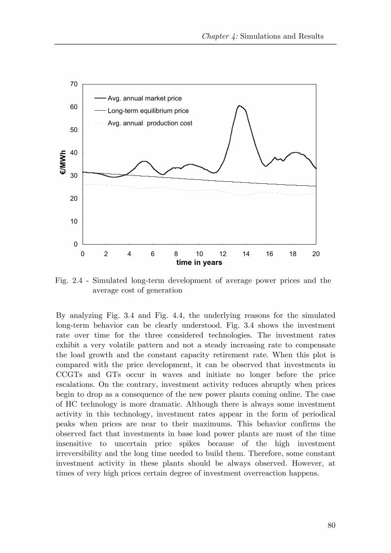
Chapter 4: Simulations and Results
80
By analyzing Fig. 3.4 and Fig. 4.4, the underlying reasons for the simulated long-term behavior can be clearly understood. Fig. 3.4 shows the investment rate over time for the three considered technologies. The investment rates exhibit a very volatile pattern and not a steady increasing rate to compensate the load growth and the constant capacity retirement rate. When this plot is compared with the price development, it can be observed that investments in CCGTs and GTs occur in waves and initiate no longer before the price escalations. On the contrary, investment activity reduces abruptly when prices begin to drop as a consequence of the new power plants coming online. The case of HC technology is more dramatic. Although there is always some investment activity in this technology, investment rates appear in the form of periodical peaks when prices are near to their maximums. This behavior confirms the observed fact that investments in base load power plants are most of the time insensitive to uncertain price spikes because of the high investment irreversibility and the long time needed to build them. Therefore, some constant investment activity in these plants should be always observed. However, at times of very high prices certain degree of investment overreaction happens.
Fig. 2.4 - Simulated long-term development of average power prices and the average cost of generation
0
10
20
30
40
50
60
70
0 2 4 6 8 10 12 14 16 18 20time in years
€/M
Wh
Avg. annual market price
Long-term equilibrium price
Avg. annual production cost

Chapter 4: Simulations and Results
81
The reason for the observed fluctuating investment behavior is that even though investors are forecasting the future reserve margin years in advance, because of the investment irreversibilities they remain reluctant to invest until they observe clear and consistent evidence of positive profitability for their projects. The primary effect of the ongoing uncertainty is the delay of investment decisions. As the new power plants need additional time to be built and to be brought online, the occurrence of price spikes associated with tight supply cannot be avoided, what ultimately triggers a wave of investments and reinforces the cyclical behavior. In Fig. 4.4, the rates at which generation capacity is brought online can be observed. As it is easy to see, they lag the investment inflow by an amount equal to the average construction time of each technology. Fig. 4.4 also includes in dashed lines the rates for each technology at which capacity should be brought on line in order to keep the system under the long-run equilibrium. It can be noticed that investments in HC power plants are much of the time significantly under the equilibrium rate. The high cost of exercising the investment option emerging from the irreversibility and the long-term uncertainties, penalizes strongly HC-investments and therefore depresses the investment rate. This creates investment opportunities for more flexible technologies such as CCGTs and GTs, which exhibit lower investment
Fig. 3.4 - Simulated investment rate in the three considered generating technologies
0
10
20
30
40
50
60
70
80
90
0 2 4 6 8 10 12 14 16 18 20
time in years
MW
/mon
th
Investment rate HCInvestment rate CCGTInvestment rate GT

Chapter 4: Simulations and Results
82
irreversibilities. It is observed that, in average, the investments in gas-fired units are significantly higher than the optimal equilibrium rate what results, finally, in a bigger participation of these technologies in the generation portfolio.
This effect can be clearly evidenced in the development of the average generation costs of Fig. 2.4 and the composition of the park’s generation mix shown in Fig 5.4. The increasing participation of gas-fired technologies is mainly caused by investment overreactions and the entry of speculative capacity at times of very profitable prices.
Fig. 4.4 - Simulated capacity completion rate and the optimal completion rate to maintain the system under the long-run equilibrium
0
10
20
30
40
50
60
70
0 2 4 6 8 10 12 14 16 18 20 time in years
Equilibrium Rate HC Completion Rate HC Equilibrium Rate CCGT
Completion Rate CCGT
Equilibrium Rate GT Completion Rate CCGT
MW
/mon
th
GT

Chapter 4: Simulations and Results
83
4.3 Sensitivity analysis
4.3.1 Demand growth rate
One of the applications of the simulation model is the answering of questions regarding the impact of changes of some exogenous variables on the long-run power market development. One of these questions is the response of the system upon an increase of the load growth above the historical rate. As the load growth is closely related to the GDP growth, this situation can happen if the economic growth experiences an acceleration. In the base case, a constant electricity demand growth rate of 1% per year was assumed. In the simulation experiment the load growth is set to 2 %/year after increasing for a period of five years from the base case level. The evolution of the load growth rate is depicted in Fig. 6.4. Additionally, the simulated expectations formed by market participants on the growth rate resulting from the TREND function are shown in the same figure.
0
5
10
15
20
0 2 4 6 8 10 12 14 16 18 20
time in years
GW
GT
CCGT
HC
Fig. 5.4 - Participation of the three considered generating technologies in the generation mix
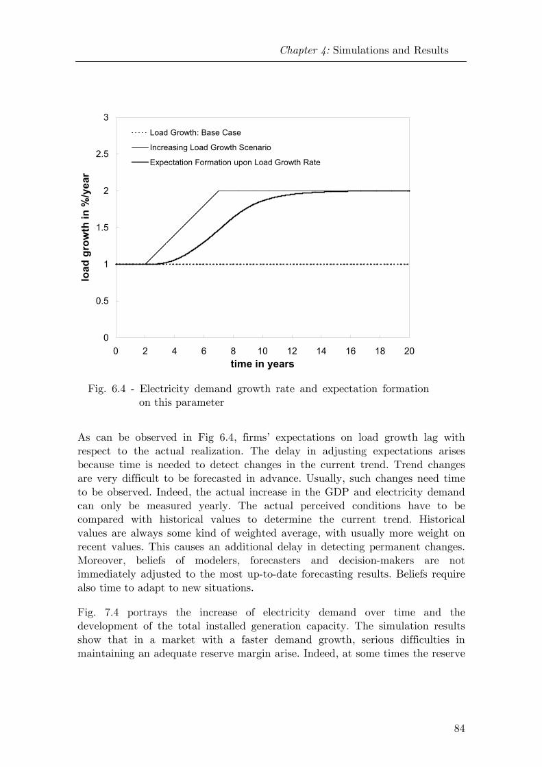
Chapter 4: Simulations and Results
84
As can be observed in Fig 6.4, firms’ expectations on load growth lag with respect to the actual realization. The delay in adjusting expectations arises because time is needed to detect changes in the current trend. Trend changes are very difficult to be forecasted in advance. Usually, such changes need time to be observed. Indeed, the actual increase in the GDP and electricity demand can only be measured yearly. The actual perceived conditions have to be compared with historical values to determine the current trend. Historical values are always some kind of weighted average, with usually more weight on recent values. This causes an additional delay in detecting permanent changes. Moreover, beliefs of modelers, forecasters and decision-makers are not immediately adjusted to the most up-to-date forecasting results. Beliefs require also time to adapt to new situations.
Fig. 7.4 portrays the increase of electricity demand over time and the development of the total installed generation capacity. The simulation results show that in a market with a faster demand growth, serious difficulties in maintaining an adequate reserve margin arise. Indeed, at some times the reserve
Fig. 6.4 - Electricity demand growth rate and expectation formation on this parameter
0
0.5
1
1.5
2
2.5
3
0 2 4 6 8 10 12 14 16 18 20time in years
load
gro
wth
in %
/yea
r
Load Growth: Base Case
Increasing Load Growth Scenario
Expectation Formation upon Load Growth Rate
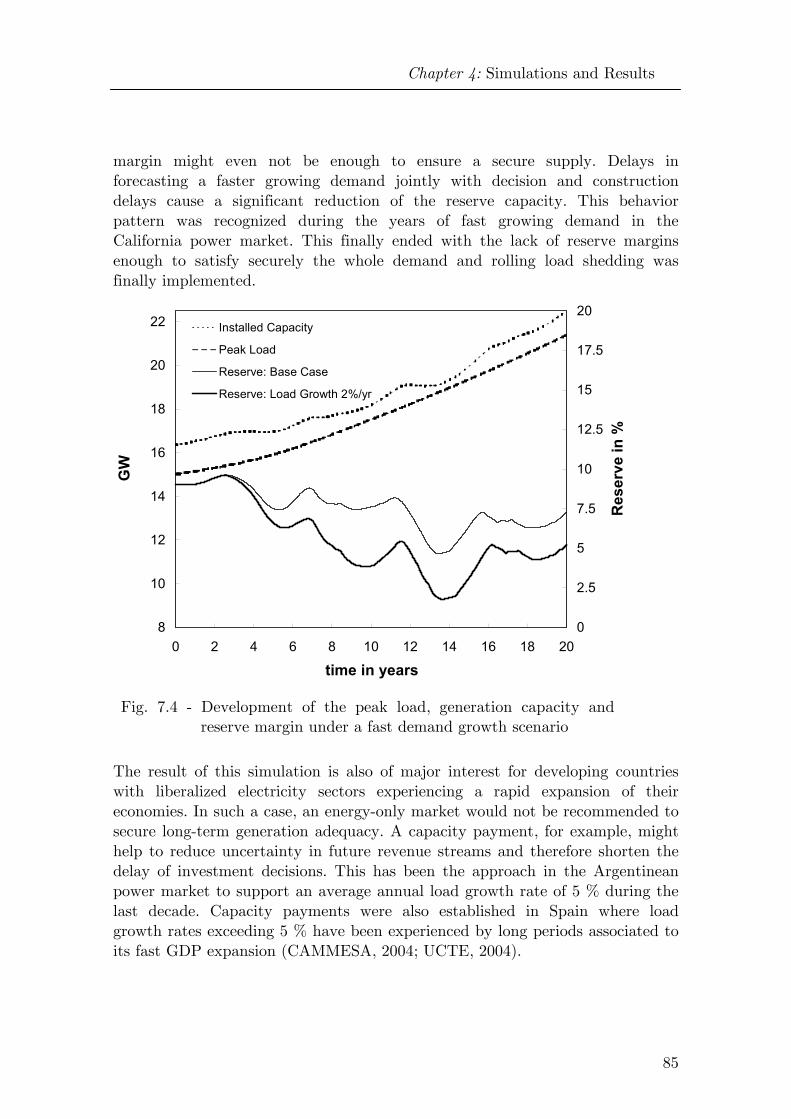
Chapter 4: Simulations and Results
85
margin might even not be enough to ensure a secure supply. Delays in forecasting a faster growing demand jointly with decision and construction delays cause a significant reduction of the reserve capacity. This behavior pattern was recognized during the years of fast growing demand in the California power market. This finally ended with the lack of reserve margins enough to satisfy securely the whole demand and rolling load shedding was finally implemented.
The result of this simulation is also of major interest for developing countries with liberalized electricity sectors experiencing a rapid expansion of their economies. In such a case, an energy-only market would not be recommended to secure long-term generation adequacy. A capacity payment, for example, might help to reduce uncertainty in future revenue streams and therefore shorten the delay of investment decisions. This has been the approach in the Argentinean power market to support an average annual load growth rate of 5 % during the last decade. Capacity payments were also established in Spain where load growth rates exceeding 5 % have been experienced by long periods associated to its fast GDP expansion (CAMMESA, 2004; UCTE, 2004).
Fig. 7.4 - Development of the peak load, generation capacity and reserve margin under a fast demand growth scenario
8
10
12
14
16
18
20
22
0 2 4 6 8 10 12 14 16 18 20
time in years
GW
0
2.5
5
7.5
10
12.5
15
17.5
20
Res
erve
in %
Installed Capacity
Peak Load
Reserve: Base Case
Reserve: Load Growth 2%/yr

Chapter 4: Simulations and Results
86
4.3.2 Setting VOLL and price cap policies
Another important application of a market simulation model is assessing the effect of regulatory policies on the long-run market development. One feasible variable to be politically influenced is the determination of the right VOLL value. This value will actually work as a price cap when markets cannot be cleared. For this reason, the numerical value for VOLL must be carefully selected as it has a decisive influence on the long-term market dynamics. Fig. 8.4 shows the long-run price development under different assumptions for VOLL.
The simulations show that average prices can significantly be reduced by setting VOLL at low values. Nevertheless, a mistake in setting VOLL can induce undesired side effects. In fact, as Fig. 9.4 illustrates, the system’s generation adequacy, which is measured by the Lost of Energy Expectation (LOEE), is
Fig. 8.4 - Simulated average market prices under different assumption for the VOLL-value
0
10
20
30
40
50
60
70
0 2 4 6 8 10 12 14 16 18 20
time in years
€/M
Wh
Market Price with VOLL set to 1000 €/MWh
Market Price with VOLL set to 500 €/MWh
Market Price with VOLL set to 250 €/MWh

Chapter 4: Simulations and Results
87
clearly damaged. In fact, investment profitability is significantly reduced when market prices are set too low for deficit conditions. In the long-run the reserve margins are thus decreased. This is indeed the case depicted in Fig. 10.4 for a dynamic price cap policy. Regulators intending to cap markets at values lower than VOLL to protect customers of high prices introduce inefficiencies on both sides of the market. On one side, the customers do not have any incentive to reduce or reallocate power demand when supply deficit arises and on the other side the long-run investment signal for generation capacity is highly disrupted. The policy of setting a price lower than the VOLL in a condition of deficit cannot be reversed easily. If the authority restores the price cap at the efficient level after relieving the deficit situation, investor in power plants might expect a low price cap if a situation of tight supply emerges again in the future. Hence, profitability expectations remain probably unaltered even after restoring the price cap to the right value. Thus, the occurrence of a new episode of capacity deficit might not be avoided and the authority would be forced to introduce again a lower price cap. This interaction between regulator and firms constitutes an important case of self-fulfilling expectations, which requires further investigation.
Fig. 9.4 - Lost of Energy Expectation (LOEE) over time under different price cap policies
0
0.00025
0.0005
0.00075
0.001
0 2 4 6 8 10 12 14 16 18 20
time in years
LOEE
in p
u
LOEE with VOLL set to 1000 €/MWh
LOEE with VOLL set to 500 €/MWh
LOEE with VOLL set to 250 €/MWh

Chapter 4: Simulations and Results
88
4.3.3 Capital costs
A last experiment carried out on the market simulator evaluates the long-run market development under different scenarios for the prevailing interest rate level. Risk-free interest rates are the determinant at each time of the required rate of return on riskless investments, such as treasury bills. The cost of capital for investments in risky assets will be greatly influenced by this parameter. In fact, capital costs as they are usually computed, will be a risk premium added to the risk-free interest rate. Investments have therefore to be discounted with this figure and thus, it represents the minimum rate of return required by investors to proceed with an investment. In the base case simulations, an average required rate of return on investments of 12.5 % at industry level was assumed, which seems to be a typical value for liberalized generation sectors. Further simulations were carried out by varying the required rate of return on investments 2.5 % in both directions. Such deviations can occur as a consequence of changes in both the interest rate levels and the perceived risk of investing at a certain time. Another important influencing factor on the RRR is the firms’ financing structures.
Fig. 10.4 - Simulation of the reserve margin under a dynamic price cap policy
0
2
4
6
8
10
12
0 2 4 6 8 10 12 14 16 18 20
time in years
Res
erve
in %
0
500
1000
1500
2000
2500
3000
VOLL
in €
/MW
h
Capacity reserve under price cap policy
Base Case
Price cap policy

Chapter 4: Simulations and Results
89
It can be noticed from Fig. 11.4, that a not very significant change in the capital cost causes a quite different system response. An increase of 2.5 % in the investors’ average hurdle rate leads to a clear worsening of the reserve margins. In contrast, a reduction in capital costs can be an effective measure to stabilize the dynamic response and to avoid costly behaviors. These results suggest some interesting reflections. It is acknowledged that long-term market efficiency can only be ensured by a reasonable degree of competition among market participants. In order to fulfill this condition, a big number of suppliers is required or what is the same, firms have to be small compared with market size. Small firms, as for example IPPs, face usually higher capital costs than big power firms holding a diversified generation portfolio. The ideal of a very fragmented supply structure composed by small IPPs might lead to costlier long-run dynamics, than a more concentrated power sector. The optimal supply structure considering the trade-off between the cost derived from long-run system’s dynamics and the costs associated with short-term firms’ strategic behaviors in a more concentrated generation industry, i.e. market power, remain yet an important open issue that call for more research effort.
Fig. 11.4 - Simulations of the reserve margin development under different hurdle rates
0
2
4
6
8
10
12
0 2 4 6 8 10 12 14 16 18 20
time in years
Res
erve
in %
Required Rate of Return 10 %
Required Rate of Return 12.5 %
Required Rate of Return 15 %
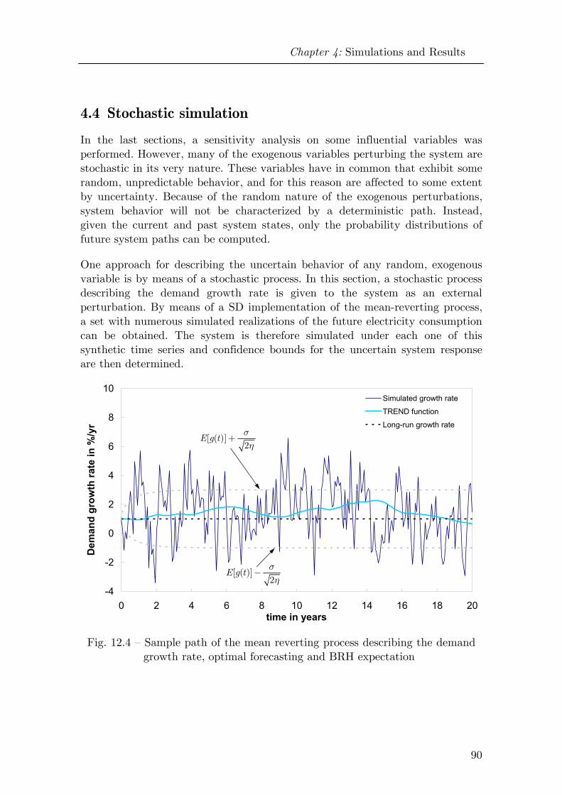
Chapter 4: Simulations and Results
90
4.4 Stochastic simulation
In the last sections, a sensitivity analysis on some influential variables was performed. However, many of the exogenous variables perturbing the system are stochastic in its very nature. These variables have in common that exhibit some random, unpredictable behavior, and for this reason are affected to some extent by uncertainty. Because of the random nature of the exogenous perturbations, system behavior will not be characterized by a deterministic path. Instead, given the current and past system states, only the probability distributions of future system paths can be computed.
One approach for describing the uncertain behavior of any random, exogenous variable is by means of a stochastic process. In this section, a stochastic process describing the demand growth rate is given to the system as an external perturbation. By means of a SD implementation of the mean-reverting process, a set with numerous simulated realizations of the future electricity consumption can be obtained. The system is therefore simulated under each one of this synthetic time series and confidence bounds for the uncertain system response are then determined.
Fig. 12.4 – Sample path of the mean reverting process describing the demand growth rate, optimal forecasting and BRH expectation
-4
-2
0
2
4
6
8
10
0 2 4 6 8 10 12 14 16 18 20time in years
Dem
and
grow
th ra
te in
%/y
r
Simulated growth rate
TREND function
Long-run growth rate
[ ( )]2
E g t ση
+
[ ( )]2
E g t ση
−

Chapter 4: Simulations and Results
91
Fig. 12.4 illustrates a sample path of the demand growth rate simulated by means of Monte Carlo methods. The optimal forecasting for this stochastic process is given by its expected value ( 1 %/yrg = ) and the 66%-confidence interval (± 1 standard deviation). This forecast is optimal and responds to the REH if the demand growth rate effectively follows a mean-reverting process. However, more than one stochastic process might adjust equally well the set of available data, impeding from forming full rational expectations on future demand growth. If knowledge is not perfect, most probably, agents pose some form of bounded rationality when forecasting. Fig. 12.4 also depicts BRH expectations formed upon the long-run demand growth by means of the TREND function.
In Fig. 13.4 simulated paths for the development of the peak load with three different seeds are shown. Although, the stochastic process remain the same, sample realizations can differ to a great extent. The market model can be run under this three load developments in order to obtain three sample simulations of key variables, such as the development of reserve margins and the average market prices. Fig. 14.4 and Fig. 15.4 depict the evolution of these variables simulated with the same seeds. The system output itself resembles the behavior of a stochastic process. Indeed, the dynamical state equations relate the exogenous stochastic processes (the inputs) with the stochastic system response (the output).
10
12
14
16
18
20
0 2 4 6 8 10 12 14 16 18 20time in years
Peak
Loa
d in
GW
Fig. 13.4 – Three sample paths of the stochastic development of the peak load

Chapter 4: Simulations and Results
92
0
2
4
6
8
10
12
0 2 4 6 8 10 12 14 16 18 20time in years
Res
erve
in %
Fig. 14.4 – Three sample paths of the stochastic development of the reserve margin
Fig. 15.4 – Three sample paths of the stochastic price development
0
20
40
60
80
100
0 2 4 6 8 10 12 14 16 18 20time in years
Ave
rage
ann
ual p
rice
in €
/MW
h

Chapter 4: Simulations and Results
93
The market dynamics can show a very different pattern depending of the particular realization of the stochastic variable. By simulating repeatedly the system under a sufficiently large number of stochastic realizations of the mean-reverting process, the general statistical properties of the market development emerge. By doing so, it is possible additionally to obtain expected values and confidence intervals for the uncertain market dynamics. The results of 100 runs simulated with an integration step of 1/8 month are shown in Fig. 16.4 and Fig. 17.4. Though in practical applications a higher number of simulations might be required to achieve a high degree of confidence, 100 runs are enough to characterize the uncertainty affecting the market dynamics.
In Fig 16.4, it is observed that the expected behavior of the reserve margin, though fluctuating, is clearly decreasing, what supports the findings of the base case simulations. However, the expected value does not exhibit a so markedly fluctuating behavior as those shown for simulations with a constant demand growth rate; see Fig. 1.4 and Fig. 7.4. It can be noticed that most of the results are concentrated around the expected path, and only a small fraction of them disperses in a seemingly wide range. It is also worth to note that, even though the variance of the demand growth rate stabilizes in the long-run, the uncertainty of the system dynamics increases steadily over time. This effect manifests stronger in the simulations of the annual average market prices of Fig. 17.4. Accordingly to the downward trend of the reserve margins, the expected value of market prices increases over time. This might pose some concern on the often claimed ability of liberalized power markets to reduce prices to end-consumers. Prices move most probably in an ostensibly narrow band, though some price scenarios with huge deviations from the mean can happen. As it can be noticed, the probability distributions of the price dynamics are highly asymmetric with respect to the mean. That is because the probability distributions are limited by the lowest marginal cost of generation of the existing power plants, as market prices cannot go below this value. In addition to this, the limiting price bound shows a decreasing trend as consequence of the progress of thermal efficiencies, and hence, cheaper base-load generation becomes available over time.
Other exogenous variables affected of uncertainty could be modeled by means of stochastic processes. Such might be the case of interest rates, availability of primary resources, fuel prices, etc. Moreover, correlations observed between variables, e.g. gas and coal prices, might be additionally taken into account. By following the steps shown previously, multivariate Monte Carlo simulations of the considered stochastic processes might be carried out and stochastic market simulations would allow determining the market dynamic uncertainty. Valuing

Chapter 4: Simulations and Results
94
power plant investments and long-term contracts under long-term market uncertainty seem straightforward applications of this stochastic market model.
0
2
4
6
8
10
12
14
16
0 2 4 6 8 10 12 14 16 18 20time in years
Res
erve
in %
50 %70 %80 %90 %Expected value
Fig. 16.4 – Uncertainty and confidence intervals for the system reserve margin
0
20
40
60
80
100
120
140
0 2 4 6 8 10 12 14 16 18 20time in years
€/M
Wh
50 %70 %80 %90 %Expected value
Fig. 17.4 – Uncertainty and confidence intervals for the average market price

95
Chapter 5 Conclusions
In the last 15 years, an active movement towards liberalization of the energy markets has been registered worldwide. Many countries have restructured their electricity industries mainly by introducing competition in their power generation sectors. Although some restructuring has been regarded as successful, the short experience accumulated with liberalized power markets does not allow making any founded assertion about their long-term behavior. Long-term prices and long-term supply reliability are now center of interest. This concerns firms considering investments in generation capacity and regulatory authorities interested in assuring the long-term adequacy and security of supply as well as the stability of power markets.
These issues have become particularly relevant because of severe, unexpected anomalies observed in some restructured markets. Most prominent is the case of the market established in California, which suffered a sustained shortage of generation capacity, which led to an energy and price crisis in summer 2000 and 2001. Inefficiencies in the resource allocation have also occurred in some markets as consequence of overbuilding. The power markets in UK and Argentina have registered low, unprofitable prices as a result of the massive entry of CCGT-based capacity. Signals of overinvestment are also currently exhibited in some U.S. markets.

Chapter 5: Conclusions
96
Deviations from the economic long-term equilibrium are not captured by standard, neoclassical partial equilibrium models. These models are based on the presumption that markets evolve as a sequence of optimal equilibrium states. Under this perspective, the market outcomes replicate the results of a centrally made optimization. However, some restrictive assumptions underlie this approach, namely perfect competition and agents behaving as inter-temporal optimizers. Rational expectations are a central hypothesis in equilibrium formulations. Nonetheless, the assumption of rational expectation precludes models from capturing deviations of the optimal equilibrium state, such as business cycles. Therefore, new market models with the ability of capturing the observed deviations from the economic equilibrium are needed.
In this thesis, a complete and self-contained mathematical methodology to simulate the long-run development of liberalized power markets has been developed. The method assumes inherently that long-term movements respond to changes in market fundamentals. Since the long-run market evolution is driven mainly by generation capacity investments, the model focuses fundamentally on the supply side. The methodology is flexible enough to consider adequately feedbacks, non-linearities and time delays present in actual markets. Additionally, the mathematical framework is suitable for being combined with Monte Carlo techniques in order to perform stochastic simulations by means of random realization of exogenous stochastic processes.
The model is based on a systemic approach, known as System Dynamics, that allows deriving the system’s dynamic response from the logical system’s structure. It was shown that these interrelationships among the different system components lead to Stochastic Delay-Differential Equations, which are responsible for endogenously generated long-term dynamics. Because of the non-linear nature, the state equations are numerically simulated. The dynamic behavior of the system is dominated by the market feedback formed by firm expectations and by the embedded delays on the balancing feedback loop. Simulation results show that investments in power plants do not keep permanently pace with demand growth and capacity retirements. Imperfect foresight, and most importantly, investment decision and construction delays prevent adjusting timely the production capacity.
This leads to fluctuating reserve margins, and consequently, to volatile long-run market prices. Some simulation experiments have additionally revealed the influence of exogenous variables on the long-run market evolution. Increasing load growth might cause additional difficulties to balance supply and demand. The application of the simulation model has proved useful to assess the impact

Chapter 5: Conclusions
97
of price cap reduction policies, which have been a repeated temptation in energy-only markets experiencing price spikes arising from capacity inadequacy. The simulation results warn strongly about the misunderstanding and abuse of these regulatory instruments. In addition to this, the effects of different industry-wide RRR were illustrated. These simulation results suggest that the optimal fragmentation of the supply side represents an important, yet unexplored topic that requires more research effort. Finally, stochastic simulations of the system under random realizations of the stochastic process governing the demand growth have proven a powerful means of representing the uncertainty of the market dynamics. Downward trend in the expected path for the reserve margin and its associated price escalation pose some concern on the ability of liberalized power markets to deliver to end-consumers cheaper electricity in the long-term.
5.1 Prospects for further research works
The developed mathematical framework is flexible enough to allow a number of extensions and refinements without much effort. Some suggestions for futures investigations would be:
The effect of some demand elasticity on the long-run system’s behavior.
The market uncertainty associated to other stochastic variables, such as interest rates, fuel prices, etc.
The analytic, asymptotic properties of the dynamic equations. For this purpose, probably the linearization of the differential equations might be necessary. Other possible approach would be the numerical mapping of the stability areas of the full, non-linear equations.
In addition, some studies of current interest, for which the developed model can contribute substantially, are suggested:
The impact of a large-scale deployment of new generating technologies, such as wind, on the development of the power market.
The long-run influence of the introduction of a CO2-certificate market on the long-run investments and prices.
Additionally, some model assumptions might be relaxed further. The price formation model could consider the increasing possibility of exercising market

Chapter 5: Conclusions
98
power under tight supply conditions and rise prices above competitive levels. Furthermore, the supply model might be extended to take into account more generating technologies, particularly hydro-storage power stations. In this context, the concept of “water value” might be valuable to facilitate the representation of hydro power plants in the supply curve.
Further investigations in the area of expectation modeling and market dynamics under learning, yet largely unexplored topics, would result in substantial contributions to the economic theory as a whole, as well as to the power system economics. Some work of the author on the field of heterogeneous expectation formations look very promising (Hübner, Olsina and Garcés, 2004).
To conclude, the simulation model here presented can be assimilated to a very sophisticated scenario generator. An interesting further extension is hence the stochastic modeling of all relevant uncertain variables, e.g. fuel prices, demand growth, interest rates, etc., by means of stochastic processes. Multiple realizations of the stochastic processes generated by a Monte Carlo SD algorithm can be supplied to the model to determine the mathematical expectations on the dynamic path followed by the system at each time point, as well as its statistical distribution. These results might be of significant value in the firm strategic planning as well as in investment appraisals of power plants projects and long-term contracting based on the Real Option approach. For this purpose, given the uncertainty of the market dynamics, a stochastic dynamic programming algorithm might be able of finding the true value of an investment opportunity, the entry threshold and the optimal time of exercising the investment option.

99
References
Alba, J. J., 2003. Investment in gas fired generation, IEA/NEA Workshop on power generation investment in liberalised electricity markets, March 25th, Paris, France.
Anderson, E. J., Philpott, A. B., 2002. Optimal offer curve construction in electricity markets. Mathematics of Operations Research, Vol. 27 (1), 82–100.
Anderson, M., Goldsmith, A., 1997. Mr. Keynes’ theory of investments: Do forward looking expectations and weight really matters? Journal of Economic Psychology, Vol. 18, 547-573.
Berends, P., Romme, A., 2001. Cyclicality of capital-intensive industries: a system dynamics study of the paper industry. Omega, Vol. 29, 543-552.
Billinton, R., Allan, R., 1996. Reliability Evaluation of Power Systems, Plenum Press, New York.
Borenstein, S., Bushnell,J., Kahn, E., Stoft, S., 1995. Market power in California electricity markets. Utilities Policy, Vol. 5 (3/4), 219–236.

References
100
Borschev, A., Filippov, A., 2004. From System Dynamics and Discrete Event to Practical Agent-based Modeling: Reasons, Techniques and Tools, Proceedings of the System Dynamics Conference, Oxford, 2004.
Boucekkine, R., Licandro, O., Paul, C., 1997. Differential-difference equations in economics: On the numerical solution of vintage capital growth models, Journal of Economics Dynamics and Control, Vol. 21, 347-362.
Bower, J., 2002. Why Did Electricity Prices Fall in England and Wales? Oxford Institute for Energy Studies, September 2002. ISBN 1 901 795 22 5. Available online at: http://econwpa.wustl.edu:8089/eps/othr/papers/0401/0401008.pdf
Bromiley, P., 1986. Corporate planning and capital investment. Journal of Economic Behavior and Organization, Vol. 7, 174-170.
Bunn, D. W., Oliveira, F. S., 2001. Agent-based simulation - an application to the new electricity trading arrangements of England and Wales, IEEE Transactions on Evolutionary Computation, Vol. 5 (5), 493-503.
Bunn, D. W., Larsen, E., 1992. Sensitivity of reserve margin to factors influencing investment behaviour in the electricity market of England and Wales, Energy Policy, Vol. 20 (5), 420-429.
CAMMESA, Compañía Adminsitradora del Mercado Mayorista Eléctrico S.A. (Argentinean Independent Sytem Operator). Statistics available at www.cammesa.com.ar
CAMMESA, 2002. Argentine Wholesale Electricity Market Annual Report. Available at: www.cammesa.com.ar
Capone, C., Capone, B., 1992. Rational entry into risky markets with negative expected returns, Journal of Economic Behavior and Organization, Vol. 18, 415-425

References
101
Caramanis, M. C, 1982. Investment decisions and long-term planning under electricity spot pricing. IEEE Transactions on Power Apparatus and Systems PAS-101(12), 4640-4648.
Chern, W. S., Just, R. E., 1982. Assessing the need for power: A regional econometric model, Energy Economics, Vol. 4 (4), 232-239.
Colpier, U. C., Cornland, D., 2002. The economics of the combined cycle gas turbine—an experience curve analysis, Energy Policy, Vol. 30 (4), 309-316.
Conlisk, J., 1996. Why Bounded Rationality? Journal of Economic Literature, Vol. 24, 669-700.
Cumperayot, P., 2004. Effects of Modeling Accuracy on System Marginal Costs Simulations in Deregulated Electricity Markets. Ph.D. Thesis, RWTH Aachen University, ABEV Series (97), Klingberg Verlag, Aachen. ISBN 3-934318-50-9.
Coyle, E., 2002. Economist’s Stories, and Culpability in Deregulation, The Electricity Journal, Vol. 15 (8), 90-96.
De Vries, L. J., Hakvoort, R. A, 2003. The question of generation adequacy in liberalized electricity markets, in Proceedings, 26th IAEE International Conference, Prague, Czech Republic, 4-7 June.
Dimson, E., 1989. The discount rate for a power station, Energy Economics, Vol. 11 (3), 175-180.
Dixit, A., Pindyck, R., 1994. Investment Under Uncertainty, Princeton University Press, Princeton.
EVA, 2002. U.S. Reserve margins expected to peak in 2004 as supply expansion continues, Energy Venture Analysis, Press release April 2002. Available online at: http://www.evainc.com/evapr-pdf/pr%20reserve_margins_apr2002.pdf

References
102
EVA, 2003. Tracking the Boom of New Power Plants in the U.S., Energy Venture Analysis, June 2003. Available online at: http://www.evainc.com/evapr-pdf/ccgt_jun2003.pdf
Evans, G. W., Honkapohja, S., 2001. Learning and Expectations in Macroeconomics, Princeton University Press, Princeton, NJ.
Farmer, R., 1997. Utility-scale combined cycle prices are leveling out after steep decline. Gas Turbine World, Vol. 27 (6), 15–20.
Farmer, R., 1999. Large combined cycle plant prices are climbing after years of decline. Gas Turbine World, Vol. 29 (1), 10–13.
Flaschel, P., Franke, R., Semmler, W., 1997. Dynamic Macroeconomics: Instability, Fluctuations, and Growth in Monetary Economies (Studies in Dynamical Economic Science), The MIT Press. ISBN 0262061910.
Ford, A., 1990. System dynamics and the electric power industry, System Dynamics Review, Vol. 13 (1), 57-81.
Ford, A., 1999. Waiting for the boom: a simulation study of power plant construction in California, Energy Policy, Vol. 29 (11), 847-869.
Forrester, J. W., 1961. Industrial Dynamics, Cambridge. MIT Press; currently available from Pegasus Communications, MA.
García, J., Román, J., Barquín, J., González, A., 1999. Strategic bidding in deregulated power systems, Proceedings of the 13th PSCC Conference, Norway.
Gross, G., Finlay, D.J., 1996. Optimal bidding strategies in competitive electricity markets, Proceedings of the 12th PSCC Conference, Germany.
Gulay Avsar, S., Goss, B. A. 2001, Forecast errors and efficiency in the US electricity futures market, Australian Economic Papers, Vol. 40 (4), 479-499.

References
103
Hensing, I., 1997. Analyse der Strompreisunterschiede zwischen Frankreich und Deutschland, Zeitschrift für Energiewirtschaft (ZfE), Band 4, 269-294.
Hoster, F., 1999. Effects of a European electricity market on the German electricity industry: results from a simulation model of the European power system, Applied Economics, Vol. 31, 107-122.
Hübner, M., Olsina, F., Garcés, F. F., 2004. Modeling long-run price expectations in electricity markets. Internal Report, Instituto de Energía Eléctrica, December.
Hunt, G. L., Sioshansi, F. P., 2002. Is there a capacity glut, and how long will it last? The Electricity Journal, Vol. 15 (7), 63-71.
IEA, 2002. Security of Supply in Electricity Markets: Evidence and Policy Issues, International Energy Agency, Energy Market Reform Series. ISBN 92-64-19805-9.
IEA, 2003. World Energy Investment Outlook 2003, International Energy Agency. ISBN 92-64-01906-5.
IEA, 2003. Power generation investment in electricity markets, International Energy Agency, Energy Market Reform Series. ISBN 92-64-1055-65.
Jansen, Y., Brognaux, C., Whitehead, J., 2003. Keeping the Lights on: Navigating Choices in European Power Generation, Report of the Boston Consulting Group, May 2003. Available online at: http://www.bcg.com/publications/files/KeepingLights%20On_rpt_May03.pdf
Johnson, B. E., 1994. Modeling energy technology choices: which investment analysis tools are appropriate? Energy Policy, Vol. 22 (10), 877-883.
Joskow, P. L., 1997. Restructuring, Competition and Regulatory Reform in the U.S. Electricity Sector, Journal of Economic Perspectives, Vol. 11 (3), 119-138.

References
104
KEMA Consulting, 2005. Review of the methodology used in NEMMCO 2003/04 minimum reserve level assessment, January. Available on line at: http://www.nemmco.com.au/powersystemops/240-0009.pdf
Koritarov, V., 2004. Real-world market representation with agents, IEEE Power & Energy, Vol. 2 (4), 39-46.
Ku, A. , 1995. Modeling Uncertainty in Electricity Capacity Planning. Ph. D. Thesis. London Business School.
Kummerow, M. A., 1999. System Dynamics Model of Cyclical Office Oversupply, Journal of Real Estate Research, Vol. 18 (1), 233-255.
Lo, K. L., McDonald, J. R., Le, T. Q., 1991. Time-of-day electricity pricing incorporating elasticity for load management purposes, International Journal of Electrical Power & Energy Systems, Vol. 13 (4), 230-239.
McDonald, N., 1978. Time lags in biological models, Lect. Notes in Biomathematics, Springer-Verlag, Berlin-Heidelberg-New York.
Maldonado, P., Palma, M., 2004. Seguridad y calidad del abastecimiento eléctrico a más de 10 años de la reforma de la industria eléctrica en países de América del Sur. Serie 72: Recursos Naturales e Infraestructura, CEPAL (United Nations). ISBN 91-1-322549-0. Available on line at: http://146.83.6.25/literatura/sistemas_potencia/lcl2158e.pdf
Miguel, J. J., Ponosov, A., Shindiapin, A., 2002. The W-transform links delay and ordinary differential equations, Functional Differential Equations, Vol. 9 (3-4), 40-73.
Modigliani, F., Miller, M. H., 1958. The cost of capital, corporation finance, and the theory of investment, American Economic Review, Vol. 48 (June), 261-297.
Morthorst, P., 1999. Capacity development and profitability of wind turbines. Energy Policy, Vol. 27, 779-787.
References
105
Muth, J., 1961. Rational expectations and the theory of price movements, Econometrica, Vol. 29, 315-335.
NEMMCO, National Electricity Market Management Company (Australia). Statistic available at: www.nemmco.com
Neuhoff, K., De Vries, L., 2004. Insufficient incentives for investment in electricity generations, Utilities Policy, Vol. 12 (4), 253-267.
Nollen, A., 2003. Lebensdaueranalysen von Kraftwerken der deutschen Elektrizitätswirtschaft. Papers of the Research Centre Jülich, Series: Energy Technology 25.
OMEL, Operador del Mercado Ibérico de Energía (Spain). Statistic available at: www.omel.es
Poskitt, R., Tomlinson, S. How are Electricity Futures Contracts Priced? A Preliminary Investigation, Working Paper, Department of Accountancy, Finance and Information Systems, University of Canterbury, New Zeland.
Pourdehnad, J., Maani, K. E., Sedehi, H., 2002. System Dynamics and Intelligent Agent-Based Simulation: Where is the Synergy? Proceedings of the 20th International Conference of the System Dynamics Society, 2002, Palermo.
Rajamaran, R., Kirsch, L., Alvarado, F., Clark, C., 2001. Optimal self-commitment under uncertain energy and reserve prices. In: Hobbs, B. F., Rothkopf, M. H., O’Neill, R. P., Chao, H.-P. (Eds.), The Next Generation of Electric Power Unit Commitment Models, International Series in Operations Research & Management Science. Kluwer Academic Publishers, Boston, 93–116.
Rostow, W., 1993. Nonlinear dynamics and economics: A historian’s perspective, in: Day, R. and P. Chen (Eds.), Nonlinear Dynamics and Evolutionary Economics, Oxford University Press, New York, 14-17.
Shampine, L. F., Thompson, S., 2001. Solving DDEs in MATLAB. Applied Numerical Mathematics, Vol. 7, 441-458.

References
106
Sharp, J. A., 1982. The dynamics of the UK chemical plant investment cycle, European Journal of Operational Research, Vol. 9, 238-247.
Schinkel, M. P., 2001. Disequilibrium theory: Reflections towards a Revival of Learning. Dissertation, Universitaire Pers Maastricht. ISBN 90-5278-333-0.
Scholl, H., 2001. Agent-based and System Dynamics modeling: A call for cross study and joint research, Proceedings of the 34th Hawaii International Conference on System Sciences, 2001.
Schwarz, H.-G., 2005. Modernisation of existing and new construction of power plants in Germany: results of an optimisation model Energy Economics, Vol. 27 (1), 113-137.
Simon, H., 1984. On the behavioral and rational foundations of Economic Dynamics. Journal of Economic Behavior and Organization, Vol. 5, 35-55.
Sterman, J., 1987. Expectation formation in behavioral simulation models. Behavioral Science, Vol. 32, 190-211.
Sterman, J., 1988. Modeling the formation of expectations: The history of energy demand forecasts, International Journal of Forecasting, Vol. 4 (2), 243-259.
Sterman, J., 1991. A Skeptic’s Guide to Computer Models, in Barney, G. O. et al. (eds.), Managing a Nation: The Microcomputer Software Catalog, Westview Press, Boulder, CO, 209-229. Available online at: http://web.mit.edu/jsterman/www/Skeptic's_Guide.pdf
Sterman, J., 2000. Business Dynamics: System Thinking and Modeling for a Complex World, McGraw Hill/Irwin, Boston.
Stoft, S., 2002. Power Systems Economics: Designing Markets for Electricity, IEEE Press/Wiley, New York.

References
107
Sweeney, J. L., 2002. The California Electricity Crisis, Hoover Institution Press Publication No. 513, ISBN 0-8179-2911-8.
UCTE, Union for the Co-ordination of Transmission of Electricity. Statistics available at www.ucte.org
Ventosa, M., Baíllo, A., Ramos, A., Rivier, M., 2005. Electricity market modeling trends, Energy Policy, Vol. 33 (7), 897-913.
Visudhiphan, P., Ilic, M. D., 2001. An agent-based approach to modeling electricity spot market, 2001 IFAC-SME Meeting Proceeding, Austria, September 6-8, 2001.
Weber, C., 2002. Das Investititonsparadox in wettbewerblichen Strommärkten, Energiewirtschaftliche Tagesfragen, Band 11, 756-759.
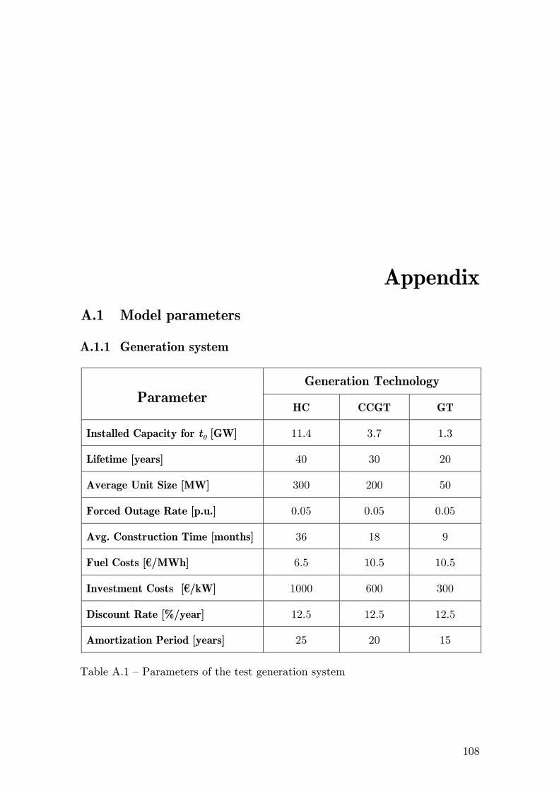
108
Appendix A.1 Model parameters
A.1.1 Generation system
Generation Technology Parameter
HC CCGT GT
Installed Capacity for t0 [GW] 11.4 3.7 1.3
Lifetime [years] 40 30 20
Average Unit Size [MW] 300 200 50
Forced Outage Rate [p.u.] 0.05 0.05 0.05
Avg. Construction Time [months] 36 18 9
Fuel Costs [€/MWh] 6.5 10.5 10.5
Investment Costs [€/kW] 1000 600 300
Discount Rate [%/year] 12.5 12.5 12.5
Amortization Period [years] 25 20 15
Table A.1 – Parameters of the test generation system

Appendix
109
A.1.2 Polynomial estimation of thermal efficiencies
HC: [ ]3 23.7676e-010 +2.7126e-007 +0.0001441 +0.455 in months t t t t−
CCGT: 4 3 23.1828e-011 +1.909e-008 4.048e-006 +0.0005138 +0.6t t t t− −
GT: 4 3 23.215e-011 +1.929e-008 4.745e-006 +0.0007222 +0.35t t t t− −
A.1.3 Electricity demand
Parameter Numerical Value
Peak Demand for t0 [MW] 15000
Lowest Demand for t0 [MW] 10000
Growth Rate [%/year] 1.00
Demand Uncertainty (Std. Dev.) [%] 1.00
VOLL [€/MWh] 1000
Table A.2 – Parameters of the demand model
A.1.4 Expectational model (TREND function)
Parameter Numerical Value
TPPC [months] 12
THRC [months] 60
TPT [months] 36
Table A.3 – Parameters for the TREND function

Appendix
110
A.1.5 Investment responsiveness (logistic function)
Numerical Value Parameter
HC CCGT GT
Saturation, maxim 1.50 3.00 2.00
Alpha, α 3.5 2.00 2.50
Beta, β -2.8069 -2.6932 -2.50
Table A.4 – Parameters of the logistic function for the investment multiplier model
A.2 SD model of the mean-reverting stochastic process
In this section, the SFD of the Ornstein-Uhlenbeck stochastic process is developed. This SD model is amenable to perform Monte Carlo simulations of the stochastic process in order to obtain a big number of realizations. The equations of the actual implementation in Vensim are also provided below.
Fig. A.1 – Stock-and-Flow Diagram of the Ornstein-Uhlenbeck stochastic process
GrowthRatedg
reversionstrenght
dzvolatility
normal variate
speed ofreversion
long-run growth<TIME STEP>
initial rate
<TIME STEP>
seed

Appendix
111
A.2.1 Model equations
Volatility ( )σ = 0.02
Speed of Reversion ( )η = 0.5
Long-run Growth ( )g = 1.00 %/year
Initial Rate = 1.00 %/year
Seed = RANDOM UNIFORM(0,1000)
Normal Variate ( )tε = RANDOM NORMAL(-100,100,0,1 seed)
Reversion Strength = (long-run Growth–Growth Rate)* Speed of Reversion* TIME STEP
dz (dz) = Normal Variate * Volatility*SQRT(TIME STEP)
dg (dg) = Reversion Strength + dz
Growth Rate (g) = INTEG(dg/TIME STEP, Initial Rate)
The values given to the stochastic process are plausible as they are in the range of the estimated values for actual systems. In the table below, the estimated parameters for different systems by means of the Ordinary Least Square (OLS) are given as comparison.
System Parameter
Argentina* Germany** Spain**
g 0.0362 0.0224 0.0409
η 0.11305 0.1558 0.5586
σ 0.01472 0.02114 0.02941
a 0.0083 0.0069 0.0296
b -0.2292 -0.3015 -0.7237
εσ 0.02788 0.03833 0.03782 * Data from CAMMESA, 76 months of observations (from Sep-98 to Dec-04) ** Data from UCTE, 168 months of observations (from Jan-91 to Dec-04) Table A.5 – Estimated parameters of the mean-reverting process for 3 countries

Appendix
112
-10%
-5%
0%
5%
10%
15%
20%
1992 1994 1996 1998 2000 2002 2004
Ann
ual g
row
th ra
te
Simulated
Fig. A.3 – Simulated realization of the mean-reverting process with estimated parameters from the Spanish system
Fig. A.2 shows the fluctuating annual growth rate for electricity demand in the Spanish power system. Fig. A.3 illustrates a simulated realization of a mean-reverting process with estimated parameters from actual data corresponding to this system.
Fig. A.2 – Actual demand growth rate in Spain
-10%
-5%
0%
5%
10%
15%
20%
1992 1994 1996 1998 2000 2002 2004
Ann
ual g
row
th ra
te
Spain

Appendix
113
A.2.2 Parameter estimation of the mean-reverting process
The Ornstein-Uhlenbeck stochastic process is given by the following expression in continues time:
( )dg g g dt dzη σ= − + (A.1)
By applying the Kolmogorov equations to this process, expressions for the mean and variance for a time interval t can be derived:
0E[ ] ( ) t
t tg g g g e η−= + − (A.2)
22[ ] (1 )
2t
tg g e ησνη
−− = − (A.3)
Eq. (A.1) is the limiting continuous version of the following first-order autoregressive AR(1) process in discrete time as 0t∆ → :
1 1(1 ) ( 1)t tt tg g g e e gη η ε− −− −− = − + − + (A.4)
where tε is normally distributed with mean zero and standard deviation εσ with:
22 2(1 )
2e η
εσση
−= − (A.5)
Parameters of Eq. (A.1) can be estimated using discrete-time data (the only data ever available) by running the regression:
1 1t tt tg g a bg ε− −− = + + (A.6)
and then computing:
2
ˆˆˆ
ˆˆ log(1 )
ˆlog(1 )ˆ ˆ ˆ(1 ) 1
agb
b
bbε
η
σ σ
= −
= − +
+=+ −
(A.7)
being ˆεσ the standard error of the regression.

114
Resumen
(Summary in Spanish)
Durante los últimos 15 años se ha registrado mundialmente un activo movimiento tendiente a la liberalización de los mercados de energía. Muchos países han reestructurado su industria eléctrica, introduciendo competencia en el segmento de generación. Aunque algunos de estos procesos han sido considerados exitosos, la corta experiencia acumulada con la liberalización de los mercados eléctricos no permite hacer afirmaciones inequívocas sobre el comportamiento de los mismos en el largo plazo. Los precios de largo plazo y la confiabilidad de suministro son ahora el foco de atención, tanto para agentes considerando hacer inversiones en generación como para autoridades regulatorias, las cuales pretenden la seguridad del suministro y la estabilidad de largo plazo de los mercados eléctricos.
Esto se ha tornado de particular relevancia luego de haberse observado severas anomalías en algunos mercados reestructurados. Es el caso del mercado establecido en California, el cual sufrió una insuficiencia sostenida de capacidad de generación que llevó a esta región a una grave crisis eléctrica durante el verano de 2000 y 2001. Ineficiencias en la asignación de los recursos han sido han observadas también en otros mercados como consecuencia de exceso de capacidad. Los mercados eléctricos de Inglaterra y Argentina han registrado la entrada masiva de capacidad basada en ciclos combinados. Señales de sobreinversión también se evidencian actualmente en algunos mercados de Estados Unidos.

Resumen (Summary in Spanish)
115
Estas desviaciones del equilibrio económico de largo plazo no son consideradas por los modelos neoclásicos de equilibrio parcial. Estos modelos presumen que los mercados evolucionan en una secuencia de estados óptimos de equilibrio. Bajo esta perspectiva, el resultado de los mecanismos de mercado replica al de una optimización global centralizada. Bajo este enfoque, subyacen, sin embargo, algunas hipótesis restrictivas, tales como condiciones de competencia perfecta y agentes cuyo comportamiento se asemeja a una optimización intertemporal. La hipótesis de expectativas racionales es central en las formulaciones de equilibrio. Sin embargo, esta conjetura imposibilita a los modelos la consideración de desviaciones del equilibrio, tales como lo son los ciclos de negocios.
Con el objetivo de lograr una comprensión acabada del comportamiento de largo plazo de los mercados eléctricos liberalizados, en esta tesis se ha desarrollado un modelo matemático basado en System Dynamics (SD). A diferencia de los modelos de mercado clásicos, este enfoque se orienta a reproducir la estructura de sistema de estos mercados y la relación lógica entre sus componentes, a fin de obtener su respuesta dinámica. En última instancia, esta estrategia se reduce a formular las ecuaciones de estado que gobiernan el comportamiento dinámico del sistema. Se muestra que la dinámica de largo plazo puede ser descripta por medio de un conjunto de ecuaciones diferenciales en retardo, las cuales son resueltas numéricamente. Esta parece ser una forma directa de modelar características estructurales inherentes a los mercados eléctricos, tales como retardos y lazos de realimentación.
Las simulaciones muestran que podrían existir problemas severos en estos mercados para ajustar la capacidad de generación y mantener estables los márgenes de reserva y los precios de mercado. Debido a la existencia de retardos sobre el mecanismo de ajuste de la oferta en el largo plazo, como por ejemplo el tiempo de construcción de nuevas centrales, la evolución podría exhibir un comportamiento volátil. Estos resultados evidencian que los mercados eléctricos son propensos a sufrir ciclos de negocios, similar a lo que ocurre en otros mercados de commodities.
La comprensión del comportamiento de largo plazo es enriquecida a partir de la realización de un análisis de sensibilidad sobre algunas variables cruciales. El crecimiento de la demanda, las tasas de interés, el nivel de concentración del mercado y los topes de precios son variables que influyen sustancialmente. Las implicancias que tienen estos resultados son discutidas al final de la tesis. Finalmente, se han llevado a cabo simulaciones estocásticas para evaluar la aptitud del modelo desarrollado para capturar la incertidumbre que afecta la dinámica de largo plazo de los actuales mercados eléctricos liberalizados.

116
Publications
Olsina, F., Haubrich, H.-J., Garcés, F., 2003. Generation capacity investment dynamics in a liberalized power market. Proceedings X ERLAC of CIGRE, Puerto Iguazú, May 2003, paper 37.10.
Olsina, F., 2003. Dynamik von Kraftwerksinvestitionen bei hoher Windenergieeinspeisung, Jahresbericht 2003, ABEV-Buchreihe, Band 92, 72-74. ISBN 3-934318-41-X.
Olsina, F., 2004. Dynamik von Kraftwerksinvestitionen bei hoher Windenergieeinspeisung, Jahresbericht 2004, ABEV-Buchreihe, Band 98, 92-95. ISBN 3-934318-52-5.
Olsina, F., Garcés, F., Haubrich, H.-J., Modeling long-term dynamics of electricity markets. Energy Policy, Elsevier Science (forthcoming). Available on line (22/12/2005) at: http://www.sciencedirect.com/science/journal/03014215
Olsina, F., Garcés, F., Cumperayot, P., 2005. Currency devaluation and long-term supply reliability of electricity markets. Proceedings XI ERIAC of CIGRE, Ciudad del Este, May 2005.
Cumperayot, P., Olsina, F., Haubrich, H.-J., 2004. Modeling Accuracy Requirements for the System Marginal Costs Simulation in Deregulated Electricity Markets. 6th IAEE European Conference on Energy Market Modelling (International Association for Energy Economics – ETH Zürich), Zurich, September 2004.

117
About the author
Fernando Olsina was born on January 27, 1976 in San Luis, Argentina. Between 1989 and 1994 he attended a technical secondary school at the ENET N°1, San Luis, where he graduated cum laude. In 1995, he began studies in Mechanical Engineering at the National University of San Juan (UNSJ), Argentina. In July 2000, he graduated cum laude. In September of the same year, he entered into the Ph.D. Program at the Institute of Electrical Energy (IEE). In April 2001, he was awarded with a four-year research fellowship from the National Research Council (CONICET) to pursue the Ph.D degree. The academic years 2002/03 and 2003/04 he spent as part of the scientific staff at the Institute of Power Systems and Power Economics (IAEW) of the Aachen University of Technology (RWTH), supported by a DAAD research fellowship. There, he developed numerous academic activities as research and teaching assistant for both, the International Master Program in Electrical Power Engineering and the Elektrotechnik Studiengang. During September/October 2004 he was lecturer of the graduate course Reliability in Competitive Power Markets. In January 2005, Mr. Olsina has submitted his application to the National Research Council aiming at joining IEE as part of the permanent research staff.
Main research fields of interest for Mr. Olsina are power market economics and modeling, expectation economics, power investment valuation and real options as well as reliability and risk management in liberalized electricity markets.