long-short portfolio optimization under cardinality constraints by difference of convex functions...

J Optim Theory Appl (2014) 161:199–224DOI 10.1007/s10957-012-0197-0

Long-Short Portfolio Optimization Under CardinalityConstraints by Difference of Convex FunctionsAlgorithm

Hoai An Le Thi · Mahdi Moeini

Received: 22 April 2012 / Accepted: 24 September 2012 / Published online: 12 October 2012© Springer Science+Business Media New York 2012

Abstract In the matter of Portfolio selection, we consider an extended version of theMean-Absolute Deviation (MAD) model, which includes discrete asset choice con-straints (threshold and cardinality constraints) and one is allowed to sell assets shortif it leads to a better risk-return tradeoff. Cardinality constraints limit the number ofassets in the optimal portfolio and threshold constraints limit the amount of capital tobe invested in (or sold short from) each asset and prevent very small investments in(or short selling from) any asset. The problem is formulated as a mixed 0–1 program-ming problem, which is known to be NP-hard. Attempting to use DC (Difference ofConvex functions) programming and DCA (DC Algorithms), an efficient approachin non-convex programming framework, we reformulate the problem in terms of aDC program, and investigate a DCA scheme to solve it. Some computational resultscarried out on benchmark data sets show that DCA has a better performance in com-parison to the standard solver IBM CPLEX.

Keywords Portfolio selection · Cardinality constraints · Threshold constraints ·Complementarity constraints · Mixed integer programming · DC programming ·DCA

1 Introduction

Given a particular amount of money, the portfolio selection problem tries to find thebest way of investing the money in a given set of assets. In this context, a portfolio

H.A. Le Thi (�)LITA, UFR-MIM, University of Lorraine, Ile du Saulcy, 57045 Metz, Francee-mail: [email protected]

M. MoeiniAlgorithms Group, Department of Computer Science, Technische Universität Braunschweig,38106 Braunschweig, Germanye-mail: [email protected]

mailto:[email protected]

mailto:[email protected]

200 J Optim Theory Appl (2014) 161:199–224

represents each one of the different ways of diversifying this money among the givenassets. In order to find the optimal portfolio, Markowitz introduced a quadratic pro-gramming model, which is called Mean-Variance (MV) model [1, 2]. For a given setof assets, the solutions of the MV model are the portfolios that offer the minimumrisk for a given level of return or maximum return for a tolerated level of risk [3–5].Konno et al. introduced a portfolio selection model, which is called Mean-AbsoluteDeviation (MAD) model [6]. It is well known that MAD model can be casted intoa linear programming problem. Hence, it can be solved much faster than the cor-responding MV model, which is a convex quadratic programming problem. Linearprogramming problems have computational advantages over quadratic programmingproblems, especially when the program contains integer variables and the dimensionof the problem is large. Furthermore, the Mean-Absolute Deviation model has an in-teresting property related to the stochastic dominance. In fact, the portfolios, whichrely on efficient frontier generated by MAD model, are efficient in the sense of sec-ond degree stochastic dominance [7, 8]. This fact is independent of the distributionof the asset return. One may note that this is, in general, not true for the Mean-Variance model. Because of these advantages of MAD model, we used the singleperiod Mean-Absolute Deviation (MAD) model proposed by Konno et al. instead ofthe Mean-Variance (MV) model employed by Markowitz.

In spite of these advantages, MAD model (as well as MV model) does not con-tain some practical constraints; for example, threshold and cardinality constraints[5, 9–11]. Cardinality constraints limit the number of stocks presented in the opti-mal portfolio and threshold constraints limit the amount of capital to be invested ineach stock and prevent very small investments in any stock. In order to overcomethese inconveniences, the MV and MAD models can be extended to include theseconstraints.

In a series of articles, Konno et al. considered an extended version of MV modeland MAD model, in which one is allowed to sell assets short, if it leads to a betterrisk-return tradeoff [12, 13]. In the same context, we generalize the MAD model inorder to take into account the cardinality and threshold constraints. The thresholdconstraints are used to limit the amount of capital to be invested in (or sold short from)each asset and prevent very small investments in (or short selling from) any asset.The cardinality constraints are included in the model for the purpose of controllingthe number of stocks (long or short) that are included in the optimal portfolio. Twotypes of cardinality constraint are used in order to have a control on the number ofthe long stocks as well as the short stocks that construct the optimal portfolio.

The generalized model can be formulated as a mixed integer programming prob-lem. This problem contains binary variables as well as some complementarity con-straints. The underlying problem is non-convex and NP-hard. The presence of theconsidered constraints is the main factor defining the level of difficulty of the prob-lem. By using an exact penalty result, we reformulate the problem in terms of a DC(Difference of Convex functions) program. A so-called DC program is that of min-imizing a DC function over a convex set. We then suggest using DC programmingapproach and DCA (DC Algorithms) to solve this portfolio selection problem. DCAwas introduced by Pham Dinh Tao in its preliminary form in 1985. It has been de-veloped extensively by Le Thi Hoai An and Pham Dinh Tao since 1994. Now, it

J Optim Theory Appl (2014) 161:199–224 201

has become classic and more and more popular (see e.g. the list of references givenin [14]). DCA has been successfully applied to many large-scale (smooth or non-smooth) non-convex programs in various domains of applied sciences, for which itprovided quite often a global solution and proved to be more robust and more efficientthan standard methods (see the list of references in [14]). For testing the efficiency ofDCA, we compare it with the standard solver IBM CPLEX.

The paper is organized as follows. After the introduction, we present in Sect. 2 themodel of the long-short portfolio selection problem under cardinality and thresholdconstraints, and its reformulation in terms of a DC program. Section 3 deals with DCprogramming and a special realization of DCA to the underlying portfolio problem.Section 4 is devoted to the implementation of the algorithm and the presentation ofthe numerical results. Some concluding remarks are drawn in Sect. 5.

2 Problem Statements and Formulation

In this paper, we adopt the MAD model introduced firstly in [6] and extensivelydeveloped in a series of the articles [6, 15–18]. Here, we are interested in an extendedMAD model that takes into account the cardinality and the threshold constraints whileselling short is allowed.

2.1 Mean-Absolute Deviation Model

First of all, let us recall the well-known Mean-Absolute Deviation (MAD) modelstudied in [6, 15–20].

Let n be the number of available assets in the market, M be the total amountof investments, and let Ri be the random variable representing the rate of returnof the ith asset. Consider a portfolio x = (x1, x2, . . . , xn) whose ith component xi

represents the amount of investment into ith asset. Assume that (R1,R2, . . . ,Rn) isdistributed over a finite set of points (r1t , r2t , . . . , rnt ) with t = 1, . . . , T and that theprobability

℘t = Pr{(R1,R2, . . . ,Rn) = (r1t , r2t , . . . , rnt )

}(1)

is known in advance. Then the expected rate of return ri of ith asset is given byri = ∑T

t=1 ℘trit , and the expected rate of return of the portfolio x is∑n

i=1 rixi .Denote by R(x) the rate of return of the portfolio x (that is,

∑ni=1 Rixi ). The

absolute deviation W [R(x)] of R(x) is defined by

W[R(x)

] = E[∣∣R(x) − E

[R(x)

]∣∣] =T∑

t=1

℘t

∣∣∣∣∣

n∑

i=1

(rit − ri)xi

∣∣∣∣∣. (2)

In what follows, we will assume, for the sake of simplicity, that ℘t = 1/T for all t .So ri = ∑T

t=1 rit /T and, consequently,

W[R(x)

] =T∑

t=1

∣∣∣∣∣

n∑

i=1

(rit − ri)xi

∣∣∣∣∣/T . (3)


Let w be a constant specifying the tolerated level of risk. The Mean-AbsoluteDeviation (MAD) model is described as follows:

max

{n∑

i=1

rixi : W[

n∑

i=1

Rixi

]

≤ wM,

n∑

i=1

xi = M,0 ≤ xi ≤ βi, i = 1, . . . , n

}

, (4)

where βi is a constant specifying the upper bound on the amount of investment intothe ith asset.

The MAD model can be reformulated as a linear programming problem by intro-ducing a set of non-negative variables vt and ut satisfying the conditions

ut − vt = ℘t

n∑

i=1

(rit − ri)xi = (1/T )

n∑

i=1

(rit − ri)xi, t = 1, . . . , T ,

and

vt ut = 0, vt ≥ 0, ut ≥ 0, t = 1, . . . , T .

These technical variables (i.e., vt and ut ) make it possible to have a well-definedlinear representation of W [R(x)] without the sign of absolute value (see [15]). Infact, with the new variables the absolute deviation W [R(x)] is represented as

W[R(x)

] =T∑

t=1

(vt + ut ).

Hence, the MAD model (4) becomes

maxn∑

i=1

rixi (5)

s.t.T∑

t=1

(vt + ut ) ≤ wM, (6)

ut − vt = (1/T )

n∑

i=1

(rit − ri)xi : t = 1, . . . , T , (7)

n∑

i=1

xi = M, (8)

vt ut = 0, vt ≥ 0, ut ≥ 0 : t = 1, . . . , T , (9)

0 ≤ xi ≤ βi : i = 1, . . . , n. (10)

In order to get a more compact formulation of the model, we first need to do a chang-ing of variables, namely vt := T vt and ut := T ut . Following these changes, the MAD


model (without transaction cost) can be written in the form

maxn∑

i=1

rixi (11)

s.t.T∑

t=1

(vt + ut )/T ≤ wM, (12)

ut − vt =n∑

i=1

(rit − ri)xi : t = 1, . . . , T , (13)

n∑

i=1

xi = M, (14)

vtut = 0, vt ≥ 0, ut ≥ 0 : t = 1, . . . , T , (15)

0 ≤ xi ≤ βi : i = 1, . . . , n. (16)

According to [15], one can leave out the complementarity constraints (i.e., vtut = 0)and the variables vt (for t = 1, . . . , T ) such that the model (11)–(16) becomes equiv-alent to the following model:

maxn∑

i=1

rixi (17)

s.t.2

T

T∑

t=1

ut ≤ wM, (18)

ut ≥n∑

i=1

(rit − ri)xi : t = 1, . . . , T , (19)

n∑

i=1

xi = M, (20)

ut ≥ 0 : t = 1, . . . , T , (21)

0 ≤ xi ≤ βi : i = 1, . . . , n. (22)

The proof and the details can be found in [15] and [20].

2.2 Extending the Model to Take into Account the Realistic Constraintsand the Short Selling Situations

The basic model (17)–(22) can be extended in order to take into account some termsrelated to the realistic situations. In what follows, we generalize the model (17)–(22)to take into account the cardinality and threshold constraints while selling assets shortis allowed.


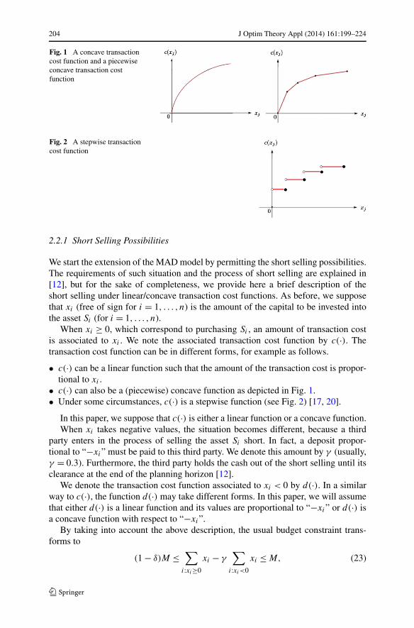
Fig. 1 A concave transactioncost function and a piecewiseconcave transaction costfunction

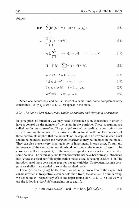
Fig. 2 A stepwise transactioncost function

2.2.1 Short Selling Possibilities

We start the extension of the MAD model by permitting the short selling possibilities.The requirements of such situation and the process of short selling are explained in[12], but for the sake of completeness, we provide here a brief description of theshort selling under linear/concave transaction cost functions. As before, we supposethat xi (free of sign for i = 1, . . . , n) is the amount of the capital to be invested intothe asset Si (for i = 1, . . . , n).

When xi ≥ 0, which correspond to purchasing Si , an amount of transaction costis associated to xi . We note the associated transaction cost function by c(·). Thetransaction cost function can be in different forms, for example as follows.

• c(·) can be a linear function such that the amount of the transaction cost is propor-tional to xi .

• c(·) can also be a (piecewise) concave function as depicted in Fig. 1.• Under some circumstances, c(·) is a stepwise function (see Fig. 2) [17, 20].

In this paper, we suppose that c(·) is either a linear function or a concave function.When xi takes negative values, the situation becomes different, because a third

party enters in the process of selling the asset Si short. In fact, a deposit propor-tional to “−xi” must be paid to this third party. We denote this amount by γ (usually,γ = 0.3). Furthermore, the third party holds the cash out of the short selling until itsclearance at the end of the planning horizon [12].

We denote the transaction cost function associated to xi < 0 by d(·). In a similarway to c(·), the function d(·) may take different forms. In this paper, we will assumethat either d(·) is a linear function and its values are proportional to “−xi” or d(·) isa concave function with respect to “−xi”.

By taking into account the above description, the usual budget constraint trans-forms to

(1 − δ)M ≤∑

i:xi≥0

xi − γ∑

i:xi<0

xi ≤ M, (23)


where δ is a small positive constant usually less than 0.02 (see [12]). In addition, thefollowing bounding constraints must be satisfied:

−α′M ≤ xi ≤ αM : i = 1, . . . , n, (24)

where α′ and α are positive constants [12].

2.2.2 Net Return of the Portfolio

In absence of the transaction costs and the commission fees, the return of the portfoliox = (x1, . . . , xn) is equal to

∑ni=1 rixi . After taking into account these costs and fees,

the expected amount of return is given by

n∑

i=1

rixi −∑

i:xi≥0

c(xi) −∑

i:xi<0

d(−xi), (25)

where c(·) and d(·) are the transaction costs functions.

2.2.3 The Long-Short MAD Model Under Transaction Costs

By introducing the set of the new constraints into the basic model (17)–(22), it istransformed to the following Long-Short model:

maxn∑

i=1

rixi −∑

i:xi≥0

c(xi) −∑

i:xi<0

d(−xi) (26)

s.t.2

T

T∑

t=1

ut ≤ wM, (27)

ut ≥n∑

i=1

(rit − ri)xi : t = 1, . . . , T , (28)

(1 − δ)M ≤∑

i:xi≥0

xi − γ∑

i:xi<0

xi ≤ M, (29)

ut ≥ 0 : t = 1, . . . , T , (30)

−α′M ≤ xi ≤ αM : i = 1, . . . , n. (31)

Let us introduce some auxiliary variables, yi and y′i such that

xi = yi − y′i , yiy

′i = 0, yi ≥ 0, y′

i ≥ 0 : i = 1, . . . , n. (32)

By using these variables, we get a model in which the proportions of the capital tobe invested in an asset (i.e., yi ) are separated from the amounts that are sold short(i.e., y′

i ). These auxiliary variables makes the model (26)–(31) to be represented as


follows:

maxn∑

i=1

(ri

(yi − y′

i

) − c(yi) − d(y′i

))(33)

s.t.2

T

T∑

t=1

ut ≤ wM, (34)

ut ≥n∑

i=1

(rit − ri)(yi − y′

i

) : t = 1, . . . , T , (35)

(1 − δ)M ≤n∑

i=1

(yi + γy′

i

) ≤ M, (36)

ut ≥ 0 : t = 1, . . . , T , (37)

0 ≤ yi ≤ αM : i = 1, . . . , n, (38)

0 ≤ y′i ≤ α′M : i = 1, . . . , n, (39)

yiy′i = 0 : i = 1, . . . , n. (40)

Since one cannot buy and sell an asset at a same time, some complementarityconstraints (i.e., yiy

′i = 0 : i = 1, . . . , n) appear in the model.

2.2.4 The Long-Short MAD Model Under Cardinality and Threshold Constraints

In some practical situations, we may need to introduce some constraints in order tohave a control on the number of the assets in the portfolio. These constraints arecalled cardinality constraints. The principal role of the cardinality constraints con-sists of limiting the number of the assets in the optimal portfolio. The presence ofthese constraints implies that the amounts of the capital to be invested in each assetshould be bounded. Hence the threshold constraints may be included in the model.They can also prevent very small quantity of investments in each asset. To sum up,in presence of the cardinality and threshold constraints, the number of assets to bechosen as well as the quantity of the invested capital in each asset are restricted tosome bounds. The cardinality and threshold constraints have been already introducedinto several classical portfolio optimization models (see, for example, [5, 9–11]). Theintroduction of these constraints requires integer variables. Consequently, some com-putational efforts are needed to solve the resulted model.

Let ai (respectively, a′i ) be the lower bound on the proportion of the capital that

can be invested in (respectively, can be sold short from) the asset Si . In a similar way,we define the bi (respectively, b′

i ) as the upper bound (for i = 1, . . . , n). So we willuse the following threshold constraints on yi and y′

i :

yi ∈ {0} ∪ [aiM,biM] and y′i ∈ {0} ∪ [

a′iM,b′

iM]. (41)


Let us define the binary variables zi and z′i (for i = 1, . . . , n) as follows:

zi = 1 iff yi ∈ [aiM,biM],0 otherwise,

and

z′i = 1 iff y′

i ∈ [a′iM,b′

iM],

0 otherwise.

In other words, zi = 1 (respectively, z′i = 1) means that the asset i is present in the

final portfolio in the long position (respectively, short position).Dealing with the portfolio optimization when short selling is allowed, we can in-

troduce two types of cardinality constraint, as follows:

Type 1: we can limit the number of the assets (either long or short) in a single cardi-nality constraint,

Type 2: we can use two separate cardinality constraints in order to control the num-ber of long assets as well as the number of the short assets in the constructedportfolio.

In what follows, we will deal with the first type. The second type of the cardinalityconstraints can be formulated in a similar way to the first type.

Let “card” denote the desired number of the assets in the optimal portfolio. TheLong-Short MAD model under cardinality constraints, so-called “MAD-card”, is for-mulated as follows:

MAD-card:

maxn∑

i=1

(ri

(yi − y′

i

) − c(yi) − d(y′i

))

s.t.2

T

T∑

t=1

ut ≤ wM,

ut ≥n∑

i=1

(rit − ri)(yi − y′

i

) : t = 1, . . . , T ,

(1 − δ)M ≤n∑

i=1

(yi + γy′

i

) ≤ M,

aiMzi ≤ yi ≤ biMzi : i = 1, . . . , n,

a′iMz′

i ≤ y′i ≤ b′

iMz′i : i = 1, . . . , n,

n∑

i=1

(zi + z′

i

) = card,

ziz′i = 0 : i = 1, . . . , n,

zi, z′i ∈ {0,1} : i = 1, . . . , n,

ut ≥ 0 : t = 1, . . . , T .

(42)


The complementarity constraints ziz′i = 0 (i = 1, . . . , n) can be replaced by

zi + z′i ≤ 1 and the resulted model can be solved by any standard integer program

(IP) solver such as IBM CPLEX. Due to the fact that the “MAD-card” is an NP-hardproblem, the resolution of the model needs some computational efforts, especiallywhen the dimension of the problem is large. Different kinds of local approach havealready been used to solve the similar NP-hard problems [5, 9, 10]. In this paperwe are interested in using a DC programming approach in order to solve the model“MAD-card” efficiently.

2.3 Reformulation of “MAD-card” as a DC Program

For formulating “MAD-card” as a DC program, we use an exact penalty result pre-sented in [21]. We will formulate “MAD-card” in the form of a convex-concave min-imization problem with linear constraints which is consequently a DC program. Inorder to simplify the notation, let

A :=

⎧⎪⎪⎪⎪⎪⎪⎪⎪⎪⎨

⎪⎪⎪⎪⎪⎪⎪⎪⎪⎩

(u,y,y′, z, z′) ∈ RT+ × R

n × Rn × [0,1]n × [0,1]n :

2T

∑Tt=1 ut ≤ wM,

ut ≥ ∑ni=1(rit − ri)(yi − y′

i ) : t = 1, . . . , T ,

aiMzi ≤ yi ≤ biMzi, a′iMz′

i ≤ y′i ≤ b′

iMz′i : i = 1, . . . , n,

(1 − δ)M ≤ ∑ni=1(yi + γy′

i ) ≤ M,∑n

i=1(zi + z′i ) = card

⎫⎪⎪⎪⎪⎪⎪⎪⎪⎪⎬

⎪⎪⎪⎪⎪⎪⎪⎪⎪⎭

.

Define the penalty function p(u,y,y′, z, z′) : R4n+T −→ R by

p(u,y,y′, z, z′) :=

n∑

i=1

(zi + z′

i

) −n∑

i=1

(zi − z′

i

)2. (43)

Furthermore, let A1 and A2 be the sets defined by

A1 = {(u,y,y′, z, z′) ∈ A : ziz

′i = 0, zi , z

′i ∈ {0,1} : i = 1, . . . , n

}

and

A2 = {(u,y,y′, z, z′) ∈ A : p(

u,y,y′, z, z′) ≤ 0}.

The reformulation of “MAD-card” as a DC program is based on the following theo-rem:

Theorem 2.1

(i) The function p(u,y,y′, z, z′) defined by (43) is concave.(ii) The function p(u,y,y′, z, z′) is non-negative on A and A1 = A2.

(iii) There is θ0 ≥ 0 such that for any θ ≥ θ0, the problem “MAD-card” is equivalentto

min{F

(u,y,y′, z, z′) : (u,y,y′, z, z′) ∈ A

}, (44)


where

F(u,y,y′, z, z′) :=

n∑

i=1

(c(yi) + d

(y′i

) − ri(yi − y′

i

)) + θp(u,y,y′, z, z′). (45)

Proof (i) Define the functions pi : R4n+T −→ R by

pi

(u,y,y′, z, z′) := (

zi + z′i

) − (zi − z′

i

)2 : ∀i = 1, . . . , n.

Define also ϕi : R4n+T −→ R by

ϕi

(u,y,y′, z, z′) := (

zi − z′i

)2 : ∀i = 1, . . . , n.

The functions ϕi are convex since they are compositions of a linear function with aconvex one. Hence, pi is sum of a linear function and a concave function, and then pi

is a concave function. On the other hand, p(u,y,y′, z, z′) := ∑ni=1 pi(u,y,y′, z, z′),

so p(u,y,y′, z, z′) is a concave function because any finite sum of concave functionsis also concave.

(ii) After rearranging the terms in (43), one can see that

p(u,y,y′, z, z′) := 2

n∑

i=1

(ziz

′i

) +n∑

i=1

zi(1 − zi) +n∑

i=1

z′i

(1 − z′

i

).

All of the right hand side terms are non-negative on A, so is p(u,y,y′, z, z′). Fur-thermore

p(u,y,y′, z, z′) = 0 ⇐⇒

⎧⎨

⎩

ziz′i = 0 : ∀i = 1, . . . , n,

zi(1 − zi) = 0 : ∀i = 1, . . . , n,

z′i (1 − z′

i ) = 0 : ∀i = 1, . . . , n,

(46)

or again

p(u,y,y′, z, z′) = 0 ⇐⇒

⎧⎨

⎩

ziz′i = 0 : ∀i = 1, . . . , n,

zi ∈ {0,1} : ∀i = 1, . . . , n,

z′i ∈ {0,1} : ∀i = 1, . . . , n.

(47)

That is{(

u,y,y′, z, z′) ∈ A : ziz′i = 0, zi, z

′i ∈ {0,1} : i = 1, . . . , n

}

= {(u,y,y′, z, z′) ∈ A : p(

u,y,y′, z, z′) = 0}.

On the other hand, p(u,y,y′, z, z′) is non-negative on A, so{(

u,y,y′, z, z′) ∈ A : p(u,y,y′, z, z′) = 0

}

= {(u,y,y′, z, z′) ∈ A : p(

u,y,y′, z, z′) ≤ 0}.

Using this fact and the relation (47) we conclude that A1 = A2.


(iii) The above property shows that the problem “MAD-card” can be expressed as

min{V

(u,y,y′, z, z′) : (u,y,y′, z, z′) ∈ A,p

(u,y,y′, z, z′) ≤ 0

}, (48)

where

V(u,y,y′, z, z′) :=

n∑

i=1

(c(yi) + d

(y′i

) − ri(yi − y′

i

)). (49)

Upon the functions c(·) and d(·), the objective function V (·) is linear or concave. Fur-thermore, A is a bounded polyhedral convex set, and p is concave and non-negativeon A. According to an exact penalty result presented in [21], there is θ0 ≥ 0 such thatfor any θ ≥ θ0, the problem (48) can be written in the form of the problem (44); inother words, (44) is equivalent to the problem “MAD-card”. This fact completes theproof of the theorem. �

Let us suppose that the functions c(·) and d(·) are linear. Under this assumption,the function F(·) is linear in variables u, y, and y′ and concave in variables z and z′.Consequently it is a DC function and a natural DC formulation of the problem (44) is

min{g(u,y,y′, z, z′) − h

(u,y,y′, z, z′) : (u,y,y′, z, z′) ∈ R

4n+T}, (50)

where

g(u,y,y′, z, z′) :=

n∑

i=1

(c(yi) + d

(y′i

) − ri(yi − y′

i

)) + χA(u,y,y′, z, z′),

and

h(u,y,y′, z, z′) := θ

(n∑

i=1

(zi − z′

i

)2 −n∑

i=1

(zi + z′

i

))

.

Here χA is the indicator function on A, i.e. χA(u,y,y′, z, z′) = 0 iff (u,y,y′,z, z′) ∈ A and +∞ otherwise.

Now suppose that at least one of the functions c(·) and d(·) is concave. Withoutloss of generality, we suppose that both of them are concave functions. In this case,the function F(·) is concave too, and a DC formulation of the problem (44) can be


(u,y,y′, z, z′) : (u,y,y′, z, z′) ∈ R

4n+T}, (51)

where

g(u,y,y′, z, z′) :=

n∑

i=1

ri(y′i − yi

) + χA(u,y,y′, z, z′),

and

h(u,y,y′, z, z′) := θ

(n∑

i=1

(zi − z′

i

)2 −n∑

i=1

(zi + z′

i

))

−n∑

i=1

(c(yi) + d

(y′i

)).


3 Solution Method via DC Programming and DCA

3.1 DCA for General DC Programs

To give the reader an easy understanding of the theory of DC programming and DCA,we first briefly outline these tools in the following. Let Γ0(R

n) denote the convexcone of all lower semicontinuous proper convex functions on R

n, and consider thegeneral DC program

(Pdc) α = inf{f (x) := g(x) − h(x) : x ∈ R

n}, (52)

where g,h ∈ Γ0(Rn). Such a function f is called DC function, and g−h, DC decom-

position of f while the convex functions g and h are DC components of f . When g

or h is a polyhedral function, (i.e., the pointwise supremum of a finite collection ofaffine functions) (Pdc) is called a polyhedral DC program which has some interestingtheoretical and practical properties.

Let C be a convex set. The problem

inf{f (x) := k(x) − h(x) : x ∈ C

}(53)

can be transformed to an unconstrained DC program by using the indicator functionon C, i.e.,

inf{f (x) := g(x) − h(x) : x ∈ R

n}, (54)

where g := k + χC .Let g∗(y) := sup{〈x,y〉 − g(x) : x ∈ R

n} be the conjugate function of g. Then, thefollowing program is called the dual program of (Pdc):

(Ddc) αD = inf{h∗(y) − g∗(y) : y ∈ R

n}. (55)

Under the natural convention in DC programming that is +∞ − (+∞) = +∞, andby using the fact that every function h ∈ Γ0(R

n) is characterized as a pointwise supre-mum of a collection of affine functions, say

h(x) := sup{〈x,y〉 − h∗(y) : y ∈ R

n},

one can prove that α = αD . We observe the perfect symmetry between primal anddual DC programs: the dual to (Ddc) is exactly (Pdc).

Recall that, for φ ∈ Γ0(Rn) and x0 ∈ domφ := {x ∈ R

n : φ(x0) < +∞}, ∂φ(x0)

denotes the subdifferential of φ at x0, i.e., (see [22])

∂φ(x0) := {y ∈ R

n : φ(x) ≥ φ(x0) + 〈x − x0,y〉,∀x ∈ Rn}. (56)

The subdifferential ∂φ(x0) is a closed and convex set in Rn. It generalizes the Fréchet

differential, in the sense that φ is differentiable at x0 if and only if ∂φ(x0) is reducedto a singleton which is exactly{∇φ(x0)}. The necessary local optimality condition forthe primal DC program (Pdc) is

∂g(x∗) ⊃ ∂h

(x∗). (57)


A point x∗ verifies the condition ∂h(x∗)∩∂g(x∗) �= ∅ is called a critical point of g−h.The condition (57) is also sufficient for many important classes of DC programs, forexample, in case of the function f is locally convex at x∗, or (Pdc) is a polyhedralDC program [23–25].

The transportation of global solutions between (Pdc) and (Ddc) is expressed bythe following propositions:

Proposition 3.1[ ⋃

y∗∈D∂g∗(y∗)

]⊂ P ,

[ ⋃

x∗∈P∂h

(x∗)

]⊂ D, (58)

where P and D denote the solution sets of (Pdc) and (Ddc), respectively.

Under technical conditions, this transportation holds also for local solutions of(Pdc) and (Ddc) (see [24–27] for more details).

Proposition 3.2 Let x∗ be a local solution to (Pdc) and let y∗ ∈ ∂h(x∗). If g∗ isdifferentiable at y∗ then y∗ is a local solution to (Ddc). Similarly, let y∗ be a localsolution to (Ddc) and let x∗ ∈ ∂g∗(y∗). If h is differentiable at x∗ then x∗ is a localsolution to (Pdc).

Based on local optimality conditions and duality in DC programming, the DCAconsists of the construction of two sequences {xk} and {yk}, candidates to be optimalsolutions of primal and dual programs, respectively, such that the sequences {g(xk)−h(xk)} and {h∗(yk) − g∗(yk)} are decreasing, and {xk} (resp. {yk}) converges to aprimal feasible solution x (resp. a dual feasible solution y) verifying local optimalityconditions and

x ∈ ∂g∗(y), y ∈ ∂h(x). (59)

The DCA then yields the next scheme:

yk ∈ ∂h(xk

); xk+1 ∈ ∂g∗(yk). (60)

In other words, these two sequences {xk} and {yk} are determined in the way thatxk+1 (resp. yk) is a solution to the convex program (Pk) (resp. (Dk)) defined by

(Pk) inf{g(x) − h

(xk

) − ⟨x − xk,yk

⟩ : x ∈ Rn}, (61)

(Dk) inf{h∗(y) − g∗(yk−1) − ⟨

y − yk−1,xk⟩ : y ∈ R

n}. (62)

In fact, at each iteration one replaces in the primal DC program (Pdc) the secondcomponent h by its affine minorization hk(x) := h(xk) + 〈x − xk,yk〉 at a neighbor-hood of xk to give birth to the convex program (Pk) whose solution set is nothing but∂g∗(yk). Likewise, the second DC component g∗ of the dual DC program (Ddc) isreplaced by its affine minorization (g∗)k(y) := g∗(yk)+〈y−yk,xk+1〉 at a neighbor-hood of yk to obtain the convex program (Dk) whose solution set is ∂h(xk+1). So,DCA performs a double linearization with the help of the subgradients of h and g∗.


It is worth noting that DCA works with the convex DC components g and h butnot the DC function f itself (see [24–27]). Moreover, a DC function f has infinitelymany DC decompositions which have crucial impacts on the performance (speed ofconvergence, robustness, efficiency, globality of computed solutions, . . . ) of DCA.

Convergence properties of DCA and its theoretical basis can be found in [24–26].For instant, it is important to mention that

– DCA is a descent method (the sequences {g(xk) − h(xk)} and {h∗(yk) − g∗(yk)}are decreasing) without linesearch.

– If the optimal value α of problem (Pdc) is finite and the infinite sequences {xk} and{yk} are bounded then every limit point x (resp. y) of the sequence {xk} (resp. {yk})is a critical point of g - h (resp. h∗ − g∗).

– DCA has a linear convergence for general DC programs.– DCA has a finite convergence for polyhedral DC programs.

In order to solve a non-convex program (Pdc) by DCA, one must search for an ap-propriate DC decomposition of the objective function of (Pdc) and also find a goodinitial point. We will apply all these procedures for solving the problem of long-short portfolio optimization under cardinality constraints which is reformulated as aDC program. We develop a DCA scheme under assumption that the transaction costfunctions (i.e., c(·) and d(·)) are linear. A similar approach can be followed for theconcave transaction cost functions (see the Appendix).

3.2 DCA for Solving the DC Program (50)

First, it is worth noting that Problem (50) is a DC polyhedral program, because g isa convex polyhedral function. According to the general framework of DCA, we firstneed computing a sub-gradient of the function h defined by

h(u,y,y′, z, z′) := θ

(n∑

i=1

(zi − z′

i

)2 −n∑

i=1

(zi + z′

i

))

.

According to the definition of h(·), it is differentiable and

(νk,vk,v′k,wk,w′k) = ∇h

(uk,yk,y′k, zk, z′k)

�νkt = 0, vk

i = 0, v′ki = 0, wk

i = θ(2(zki − z′k

i

) − 1), w′k

i = θ(2(z′ki − zk

i

) − 1),

(63)

for all i = 1, . . . , n and t = 1, . . . , T .Secondly, we must compute an optimal solution of the following linear program:

min{Fk(O) : (u,y,y′, z, z′) ∈ A

}, (64)

where

O := (u,y,y′, z, z′),


and

Fk(O) :=n∑

i=1

(c(yi)+d

(y′i

)−ri(yi −y′

i

))− ⟨(u,y,y′, z, z′k,vk,v′k,wk,w′k)⟩. (65)

The corresponding solution vector will be (uk+1,yk+1,y′k+1, zk+1, z′k+1).To sum up, the DCA applied to (50) can be described as follows.

Algorithm (Algorithm DCA for the Program (50))

– Step 1: Let ε be a sufficiently small positive number, choose an initial point suchas (u0,y0,y′0, z0, z′0) ∈ R

4n+T , define k as the iteration indicator and set k = 0;– Step 2:

For i = 1, . . . , n and t = 1, . . . , T , setνkt = 0,

vki = 0,

v′ki = 0,

wki = θ(2(zk

i − z′ki ) − 1),

w′ki = θ(2(z′k

i − zki ) − 1).

Define

O := (u,y,y′, z, z′),

and

Fk(O) :=n∑

i=1

(c(yi) + d

(y′i

) − ri(yi − y′

i

)) − ⟨(u,y,y′, z, z′k,vk,v′k,wk,w′k)⟩,

and solve the following linear program:

min{Fk(O) : (u,y,y′, z, z′) ∈ A

},

to obtain (uk+1,yk+1,y′k+1, zk+1, z′k+1).– Step 3: If ‖uk+1 − uk‖ + ‖yk+1 − yk‖ + ‖y′k+1 − y′k‖ + ‖zk+1 − zk‖ +

‖z′k+1 − z′k‖ ≤ ε, then stop, the stopping criterion is met and (uk+1,yk+1,y′k+1,

zk+1, z′k+1) is an optimal solution, otherwise set k = k + 1 and go to Step 2.

Theorem 3.1 (Convergence Theorem of DCA for Solving (50))

(i) Algorithm DCA generates a sequence {(uk,yk,y′k, zk, z′k)} contained in the ver-tex set of A such that the sequence {F(uk,yk,y′k, zk, z′k)} is decreasing.

(ii) The sequence {(uk,yk,y′k, zk, z′k)} converges, after a finite number of iterations,to the point (u, y, y′, z, z′) which is a critical point of the problem (50).

(iii) Moreover, the point (u, y, y′, z, z′) is almost always a local minimizer of Problem(50).

(iv) There is a number θ1 ≥ 0 such that for θ > θ1, the sequence {p(uk,yk,y′k,zk, z′k)} is decreasing. In particular, if (ur ,yr ,y′r , zr , z′r ) is a feasible solutionof “MAD-card” then (uk,yk,y′k, zk, z′k), for k ≥ r , is feasible too.


Proof (i) and (ii) are immediate consequences of DCA’s convergence theorem for apolyhedral DC program (see [23, 25–27]).

(iii) Consider the DC program (50), we first note that g is a polyhedral con-vex function, so is g∗. Hence, g∗ is almost always differentiable. It follows that(ν, v, v′, w, w′), the limit point of the sequence {(νk,vk,v′k,wk,w′k)}, is almost al-ways a local solution to the dual DC program of (50) (see the previous subsection).Using Proposition 3.2 in the previous subsection and taking into account the fact thath is differentiable everywhere, we conclude that (u, y, y′, z, z′) is almost always alocal solution to the problem (50).

(iv) Let V (A) be the vertex set of A. If V (A) is contained in the feasible set of“MAD-card” then θ1 = 0 (see [21]). Otherwise, let

ξ := min{p(u, y, y′, z, z′) − p

(u,y,y′, z, z′)

: ((u, y, y′, z, z′),(u,y,y′, z, z′)) ∈ V (A) × V (A),p

(u, y, y′, z, z′)

> p(u,y,y′, z, z′)},

and

η := max

{[n∑

i=1

(c(yi) + d

(y′

i

) − ri(yi − y′

i

)) −n∑

i=1

(c(yi) + d

(y′i

) − ri(yi − y′

i

))]

: ((u, y, y′, z, z′),(u,y,y′, z, z′)) ∈ V (A) × V (A)

}

,

then 0 < ξ < ∞ and 0 ≤ η < ∞, since V (A) is a finite set. Consider now the non-negative number θ1 defined by

θ1 := η

ξ

and set θ > θ1. Let {(uk,yk,y′k, zk, z′k)} be the sequence generated by DCA appliedto (50), with θ > max{θ0, θ1}. Assume by contradiction that there is r ≥ 1 such thatp(ur+1,yr+1,y′r+1, zr+1, z′r+1) > p(ur ,yr ,y′r , zr , z′r ). Since θ > θ1, we have

θ[p(ur+1,yr+1,y′r+1, zr+1, z′r+1) − p

(ur ,yr ,y′r , zr , z′r)]

> θ1[p(ur+1,yr+1,y′r+1, zr+1, z′r+1) − p

(ur ,yr ,y′r , zr , z′r)],

or

θ[p(ur+1,yr+1,y′r+1, zr+1, z′r+1) − p


>η

ξ

[p(ur+1,yr+1,y′r+1, zr+1, z′r+1) − p

(ur ,yr ,y′r , zr , z′r)].

According to the definition of ξ ,

ξ ≤ [p(ur+1,yr+1,y′r+1, zr+1, z′r+1) − p

(ur ,yr ,y′r , zr , z′r)],


so

θ[p(ur+1,yr+1,y′r+1, zr+1, z′r+1) − p

(ur ,yr ,y′r , zr , z′r)] > η.

Hence, by considering the definition of η, we have

θ[p(ur+1,yr+1,y′r+1, zr+1, z′r+1) − p


>

n∑

i=1

(c(yri

) + d(y′ri

) − ri(yri − y′r

i

))

−n∑

i=1

(c(yr+1i

) + d(y′r+1i

) − ri(yr+1i − y′r+1

i

))

i.e.,

n∑

i=1

(c(yr+1i

) + d(y′r+1i

) − ri(yr+1i − y′r+1

i

)) + θp(ur+1,yr+1,y′r+1, zr+1, z′r+1)

>

n∑

i=1

(c(yri

) + d(y′ri

) − ri(yri − y′r

i

)) + θp(ur ,yr ,y′r , zr , z′r).

This is not possible because {F(uk,yk,y′k, zk, z′k)} is a decreasing sequence and

F(uk,yk,y′k, zk, z′k) :=

n∑

i=1

(c(yki

)+d(y′ki

)−ri(yki −y′k

i

))+θp(uk,yk,y′k, zk, z′k).

In particular, if (ur ,yr ,y′r , zr , z′r ) is a feasible solution of “MAD-card”, then thesolution (uk,yk,y′k, zk, z′k) is feasible too, for k ≥ r . �

3.3 Finding a Good Initial Point for DCA

Finding a good initial point is an important issue in the design of DCA. The ques-tion is still open and it may depend on different factors. In this work, we solve therelaxed problem of “MAD-card” which is obtained by eliminating the complemen-tarity constraints and replacing the binary constraints by their continuous relaxation.The resulted model is a linear program (LP) that can be solved efficiently by usingany standard LP solver. Then the optimal solution of the relaxed problem is used forstarting DCA.

In fact, we have tested DCA by using different initial points:

– The optimal solution of the relaxed problem (as described above),– The vector 0 = (0, . . . ,0),– The vector (u0,y0,y′0, z0, z′0) such that u0 = y0 = y′0 = 0 and z0 = z′0 = 1 =

(1, . . . ,1).

In our experiments the first procedure gives the best initial point for DCA.


4 Implementation and Computational Experiments

The algorithm is coded in C++ and run on an Intel Core i3 2.40 GHz of 4.00 GBRAM. At each iteration of the algorithm, we need to solve one linear program forwhich we used the standard solver IBM CPLEX version 12.2.

We compare our algorithm with the standard IBM CPLEX applied to Mixed In-teger Linear Programming problems. For solving the problem “MAD-card” by IBMCPLEX, we replace the complementarity constraints by the linear constraints (seeSect. 2.2).

Two sets of experiments have been carried out depending on the type of the cardi-nality constraints (see Sect. 2.2):

Type 1: A single cardinality constraint is used:∑n

i=1(zi +z′i ) = card. This constraint

contains a single parameter, i.e., card.Type 2: Two separate cardinality constraints are used in order to control the number

of long assets as well as the number of the short assets in the optimal port-folio:

∑ni=1 zi = card1 and

∑ni=1 z′

i = card2. Two different parameters (i.e.,card1 and card2) are present in these constraints.

We have tested the algorithm on three data sets. They have been already used in[20] and [28] and the set of prices is publicly available at http://people.brunel.ac.uk/~mastjjb/jeb/orlib/indtrackinfo.html. The data sets correspond to weekly prices ofassets since March 1992 during 289 weeks. More precisely, we have the foollowing.

– The first data set corresponds to the index S&P 500. The number n of differentassets is 457 and T is 289.

– The second data set corresponds to the index Russell 2000. The number n of dif-ferent assets is 1318 and T is 289.

– The third data set corresponds to the index Russell 3000. The number n of differentassets is 2151 and T is 289.

In accordance to [12, 17, 20], the value of the different parameters of the modelhave been chosen as follows:

– the initial capital, M , has been considered to be equal to 10000,– the tolerated level of risk, ω, has been considered to be 5 percent of the initial

capital,– the deposit coefficient, γ , has been considered to be equal to 0.3,– δ = 0.005.

The transaction cost for buying and selling any asset is chosen to be just 1 % ofthe transaction. Finally, the lower bound parameters (ai and a′

i ) and upper boundsparameters (bi and b′

i ) have been fixed to 0.01 and 1.0, respectively.The tolerance ε for DCA is set to 10−6 and IBM CPLEX is stopped when it finds

a solution with a precision of 0.001.The parameter θ0 is an input to the DCA. In general it is not evident to compute an

exact value of θ0. In practice, we choose a sufficiently large value of θ0 to make surethat for any θ ≥ θ0, the DC program (44) is equivalent to the optimization problem“MAD-card”. For this aim, we take θ0 such that the solution provided by DCA is

http://people.brunel.ac.uk/~mastjjb/jeb/orlib/indtrackinfo.html

http://people.brunel.ac.uk/~mastjjb/jeb/orlib/indtrackinfo.html


Table 1 Numerical results for the first data set with single cardinality parameter (n = 457, T = 289)

card CPLEX DCA Gap

Optval Time Long Short Optval Time Iter. Long Short

3 5.149172 50.154 3 0 3.611798 3.432 2 3 0 0.425655

4 6.021531 18.961 4 0 4.330015 3.428 2 4 0 0.390649

5 6.661686 8.425 5 0 6.097925 3.394 2 5 0 0.092451

6 7.019929 8.176 5 1 5.068218 3.655 2 6 0 0.385088

7 7.184315 7.042 6 1 6.109270 3.748 2 7 0 0.175969

8 7.234140 3.575 7 1 6.523110 3.658 2 7 1 0.109002

9 7.265063 1.729 8 1 7.265063 3.743 2 8 1 0.000000

10 7.250300 1.723 9 1 7.250300 3.679 2 9 1 0.000000

Range – 1.7–50.1 – – – 3.4–3.8 – – – 0–0.425

integer, i.e. it is feasible to the problem “MAD-card”. In such case, according toTheorem of exact penalty in [21], we have the equivalence between (44) and “MAD-card”. In these computational experiments, θ0 = 100 is chosen for the first data setand θ0 = 1000 for the other data sets. With these choices, integrality of the solutionsprovided by DCA is guaranteed.

4.1 The Numerical Results

The results of the experiments are shown in Tables 1–6. In these tables, the perfor-mance of DCA versus IBM CPLEX is depicted via the optimal value given by eachalgorithm (Optval), the CPU time in seconds (Time), the number of DCA iterations(Iter.), the number of long assets (Long) and the number of the short assets (Short)in the optimal portfolio, and the gap of optimal values given by the two algorithms(Gap). In fact, Gap := (CPLEX’s Optval − DCA’s Optval)/DCA’s Optval.

We first present in Tables 1, 2 and 3 the results corresponding to the Type 1 of thecardinality constraints with different values of card.

According to the numerical results, the problem is difficult to solve when the valueof card is small. The problem becomes more difficult when the value of card is smalland n is large. The use of efficient local approaches such as DCA is recommended insuch a case.

When the cardinality number varies, DCA demonstrates a kind of robustness insolving the problem. This observation can be referred to low number of iterationsas well as stability in computational time. When the value of card changes, thereis no tremendous influence on the computational time of DCA. Furthermore, DCAprovides high quality solutions in a shorter time, especially for the higher dimensions.A view on the column “Gap” certifies this claim. When the value of card increasessuch that it approaches to 10, solving the corresponding problem becomes easier. Inthese cases, DCA provides a global solution. For card > 10, the problems can be(globally) solved by DCA without any computational effort.


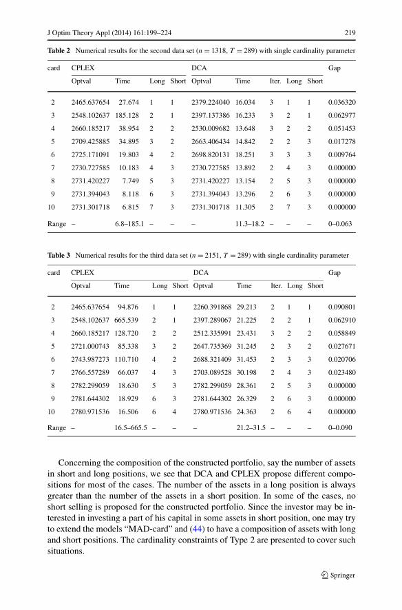
Table 2 Numerical results for the second data set (n = 1318, T = 289) with single cardinality parameter

card CPLEX DCA Gap


2 2465.637654 27.674 1 1 2379.224040 16.034 3 1 1 0.036320

3 2548.102637 185.128 2 1 2397.137386 16.233 3 2 1 0.062977

4 2660.185217 38.954 2 2 2530.009682 13.648 3 2 2 0.051453

5 2709.425885 34.895 3 2 2663.406434 14.842 2 2 3 0.017278

6 2725.171091 19.803 4 2 2698.820131 18.251 3 3 3 0.009764

7 2730.727585 10.183 4 3 2730.727585 13.892 2 4 3 0.000000

8 2731.420227 7.749 5 3 2731.420227 13.154 2 5 3 0.000000

9 2731.394043 8.118 6 3 2731.394043 13.296 2 6 3 0.000000

10 2731.301718 6.815 7 3 2731.301718 11.305 2 7 3 0.000000

Range – 6.8–185.1 – – – 11.3–18.2 – – – 0–0.063

Table 3 Numerical results for the third data set (n = 2151, T = 289) with single cardinality parameter

card CPLEX DCA Gap


2 2465.637654 94.876 1 1 2260.391868 29.213 2 1 1 0.090801

3 2548.102637 665.539 2 1 2397.289067 21.225 2 2 1 0.062910

4 2660.185217 128.720 2 2 2512.335991 23.431 3 2 2 0.058849

5 2721.000743 85.338 3 2 2647.735369 31.245 2 3 2 0.027671

6 2743.987273 110.710 4 2 2688.321409 31.453 2 3 3 0.020706

7 2766.557289 66.037 4 3 2703.089528 30.198 2 4 3 0.023480

8 2782.299059 18.630 5 3 2782.299059 28.361 2 5 3 0.000000

9 2781.644302 18.929 6 3 2781.644302 26.329 2 6 3 0.000000

10 2780.971536 16.506 6 4 2780.971536 24.363 2 6 4 0.000000

Range – 16.5–665.5 – – – 21.2–31.5 – – – 0–0.090

Concerning the composition of the constructed portfolio, say the number of assetsin short and long positions, we see that DCA and CPLEX propose different compo-sitions for most of the cases. The number of the assets in a long position is alwaysgreater than the number of the assets in a short position. In some of the cases, noshort selling is proposed for the constructed portfolio. Since the investor may be in-terested in investing a part of his capital in some assets in short position, one may tryto extend the models “MAD-card” and (44) to have a composition of assets with longand short positions. The cardinality constraints of Type 2 are presented to cover suchsituations.


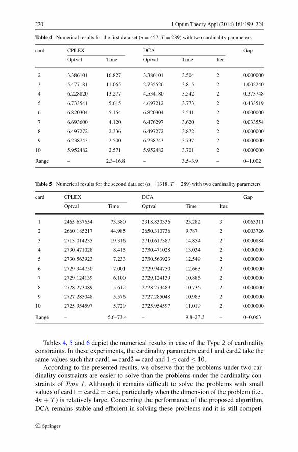
Table 4 Numerical results for the first data set (n = 457, T = 289) with two cardinality parameters

card CPLEX DCA Gap

Optval Time Optval Time Iter.

2 3.386101 16.827 3.386101 3.504 2 0.000000

3 5.477181 11.065 2.735526 3.815 2 1.002240

4 6.228820 13.277 4.534180 3.542 2 0.373748

5 6.733541 5.615 4.697212 3.773 2 0.433519

6 6.820304 5.154 6.820304 3.541 2 0.000000

7 6.693600 4.120 6.476297 3.620 2 0.033554

8 6.497272 2.336 6.497272 3.872 2 0.000000

9 6.238743 2.500 6.238743 3.737 2 0.000000

10 5.952482 2.571 5.952482 3.701 2 0.000000

Range – 2.3–16.8 – 3.5–3.9 – 0–1.002

Table 5 Numerical results for the second data set (n = 1318, T = 289) with two cardinality parameters

card CPLEX DCA Gap


1 2465.637654 73.380 2318.830336 23.282 3 0.063311

2 2660.185217 44.985 2650.310736 9.787 2 0.003726

3 2713.014235 19.316 2710.617387 14.854 2 0.000884

4 2730.471028 8.415 2730.471028 13.034 2 0.000000

5 2730.563923 7.233 2730.563923 12.549 2 0.000000

6 2729.944750 7.001 2729.944750 12.663 2 0.000000

7 2729.124139 6.100 2729.124139 10.886 2 0.000000

8 2728.273489 5.612 2728.273489 10.736 2 0.000000

9 2727.285048 5.576 2727.285048 10.983 2 0.000000

10 2725.954597 5.729 2725.954597 11.019 2 0.000000

Range – 5.6–73.4 – 9.8–23.3 – 0–0.063

Tables 4, 5 and 6 depict the numerical results in case of the Type 2 of cardinalityconstraints. In these experiments, the cardinality parameters card1 and card2 take thesame values such that card1 = card2 = card and 1 ≤ card ≤ 10.

According to the presented results, we observe that the problems under two car-dinality constraints are easier to solve than the problems under the cardinality con-straints of Type 1. Although it remains difficult to solve the problems with smallvalues of card1 = card2 = card, particularly when the dimension of the problem (i.e.,4n + T ) is relatively large. Concerning the performance of the proposed algorithm,DCA remains stable and efficient in solving these problems and it is still competi-


Table 6 Numerical results for the third data set (n = 2151, T = 289) with two cardinality parameters

card CPLEX DCA Gap


1 2465.637654 273.238 2181.402586 91.848 4 0.130299

2 2660.185217 223.114 2492.227720 27.523 2 0.067392

3 2734.563129 67.747 2668.232553 29.935 2 0.024859

4 2766.312198 31.848 2701.946665 28.782 2 0.023822

5 2780.713000 18.079 2780.713000 25.121 2 0.000000

6 2778.919470 14.137 2778.919470 22.518 2 0.000000

7 2777.092774 10.757 2777.092774 18.754 2 0.000000

8 2775.181182 10.534 2775.181182 18.494 2 0.000000

9 2772.658118 10.392 2772.658118 18.861 2 0.000000

10 2769.822095 10.554 2769.822095 18.527 2 0.000000

Range – 10.4–273.2 – 18.5–91.9 – 0–0.130

tive with CPLEX. Particularly, we observe that DCA provides a global solution forcard1 = card2 = 2 in just 2 iterations and in a very short time in comparison to thesolver CPLEX (see Table 4).

5 Concluding Remarks

In this paper, we presented a new model for portfolio selection problem and a novelapproach for solving the model. We have used the Mean Absolute Deviation (MAD)as the measure of risk. The MAD has some remarkable advantages over variance(standard deviation) that has been proposed in 50 s by H. Markowitz. The basic MADmodel is rather simple and cannot correspond to practical situations; hence, insteadof the standard formulation, we used an extension of the MAD model, including car-dinality and threshold constraints. These constraints render the MAD model morerealistic. Furthermore we have admitted the short selling situations in the model ifit provides a better risk-return tradeoff. The set of these constraints make the corre-sponding portfolio selection problem non-convex and so very difficult to solve by ex-isting algorithms. We have transformed this model into a mixed integer program withcomplementarity constraints. The resulted model has been casted into a DC (Differ-ence of Convex functions) program by using a new penalty function. The introducedpenalty function takes into account the integrality constraints as well as complemen-tarity constraints. By using this penalty function, we have more compact formulationof the DC program. After presenting the DC formulation of the problem, we devel-oped a deterministic approach based on DC programming and DCA (DC Algorithms)to solve the resulted model. It is worth noting that a mixed integer formulation of themodel can be solved by the standard solver IBM CPLEX. But using IBM CPLEX forsolving large instances of the model may not be feasible. The use of efficient localapproaches such as DCA is recommended in such cases.


Numerical experiments have been carried out by using some benchmark and pub-licly available data sets. As a final remark, we observed that, from a computationalpoint of view, our proposed approach is more efficient, robust, and inexpensive incomparison to the standard solver IBM CPLEX.

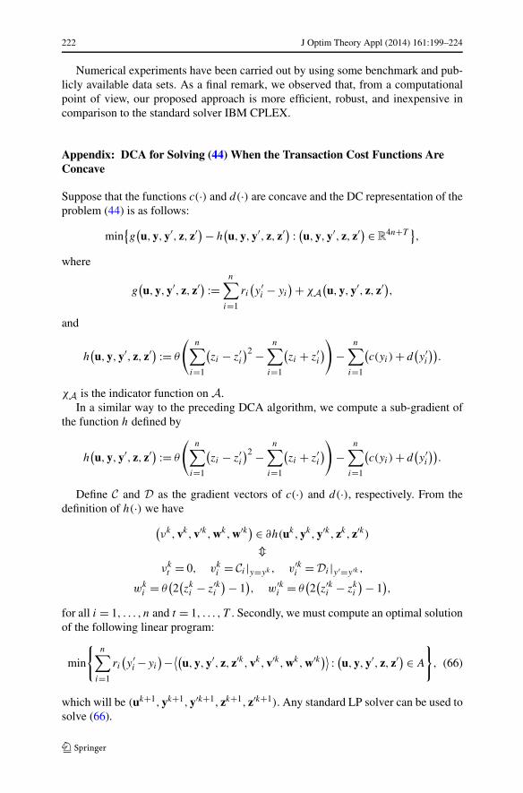
Appendix: DCA for Solving (44) When the Transaction Cost Functions AreConcave

Suppose that the functions c(·) and d(·) are concave and the DC representation of theproblem (44) is as follows:


(u,y,y′, z, z′) : (u,y,y′, z, z′) ∈ R

4n+T},

where

g(u,y,y′, z, z′) :=

n∑

i=1

ri(y′i − yi

) + χA(u,y,y′, z, z′),

and

h(u,y,y′, z, z′) := θ

(n∑

i=1

(zi − z′

i

)2 −n∑

i=1

(zi + z′

i

))

−n∑

i=1

(c(yi) + d

(y′i

)).

χA is the indicator function on A.In a similar way to the preceding DCA algorithm, we compute a sub-gradient of

the function h defined by

h(u,y,y′, z, z′) := θ

(n∑

i=1

(zi − z′

i

)2 −n∑

i=1

(zi + z′

i

))

−n∑

i=1

(c(yi) + d

(y′i

)).

Define C and D as the gradient vectors of c(·) and d(·), respectively. From thedefinition of h(·) we have

(νk,vk,v′k,wk,w′k) ∈ ∂h(uk,yk,y′k, zk, z′k)

�νkt = 0, vk

i = Ci |y=yk , v′ki = Di |y′=y′k ,

wki = θ

(2(zki − z′k

i

) − 1), w′k

i = θ(2(z′ki − zk

i

) − 1),

for all i = 1, . . . , n and t = 1, . . . , T . Secondly, we must compute an optimal solutionof the following linear program:

min

{n∑

i=1

ri(y′i −yi

)− ⟨(u,y,y′, z, z′k,vk,v′k,wk,w′k)⟩ : (u,y,y′, z, z′) ∈ A

}

, (66)

which will be (uk+1,yk+1,y′k+1, zk+1, z′k+1). Any standard LP solver can be used tosolve (66).


To sum up, the DCA algorithm will be as follows:

Algorithm (Algorithm DCA for the Program (44) When the Transaction Cost Func-tions Are Concave)

– Step 1: Let ε be a sufficiently small positive number, choose an initial point suchas (u0,y0,y′0, z0, z′0) ∈ R

4n+T , define k as the iteration indicator and set k = 0;– Step 2:

For i = 1, . . . , n and t = 1, . . . , T , setνkt = 0,

vki = Ci |y=yk ,

v′ki = Di |y′=y′k ,

wki = θ(2(zk

i − z′ki ) − 1),

w′ki = θ(2(z′k

i − zki ) − 1),

and solve the following linear program:

min

{n∑

i=1

ri(y′i − yi

) − ⟨(u,y,y′, z, z′k,vk,v′k,wk,w′k)⟩ : (u,y,y′, z, z′) ∈ A

}

,

to obtain (uk+1,yk+1,y′k+1, zk+1, z′k+1).– Step 3: If ‖uk+1 − uk‖ + ‖yk+1 − yk‖ + ‖y′k+1 − y′k‖ + ‖zk+1 − zk‖ +

‖z′k+1 − z′k‖ ≤ ε, then stop, the stopping criterion is met and (uk+1,yk+1,y′k+1,

zk+1, z′k+1) is an optimal solution, otherwise set k = k + 1 and go to Step 2.

References

1. Markowitz, H.M.: Portfolio selection. J. Finance 7(1), 77–91 (1952)2. Markowitz, H.M.: Portfolio Selection. Wiley, New York (1959)3. Bartholomew-Biggs, M.: Nonlinear Optimization with Financial Applications. Kluwer Academic,

Norwell (2005)4. Elton, E.J., Grubner, M.J., Brown, S.J., Goetzmann, W.N.: Modern Portfolio Theory and Investment

Analysis. Wiley, New York (2003)5. Fernandez, A., Gomez, S.: Portfolio selection using neural networks. Comput. Oper. Res. 34, 1177–

1191 (2007)6. Konno, H., Yamazaki, H.: Mean-absolute deviation portfolio optimization model and its applications

to Tokyo stock market. Manag. Sci. 37, 519–531 (1991)7. Ogryczak, W., Ruszczynski, A.: From stochastic dominance to mean-risk model: semi-deviations as

risk measures. Eur. J. Oper. Res. 116, 33–50 (1999)8. Ogryczak, W., Ruszczynski, A.: On consistency of stochastic dominance and mean-semi deviation

models. Math. Program. 89, 217–232 (2001)9. Chang, T.J., Meade, N., Beasley, J.E., Sharaiha, Y.M.: Heuristics for cardinality constrained portfolio

optimization. Comput. Oper. Res. 27, 1271–1302 (2000)10. Jobst, N., Horniman, M., Lucas, C., Mitra, G.: Computational aspects of alternative portfolio selection

models in the presence of discrete asset choice constraints. Quant. Finance 1, 1–13 (2001)11. Le Thi, H.A., Moeini, M., Pham Dinh, T.: Portfolio selection under downside risk measures and

cardinality constraints based on DC programming and DCA. Comput. Manag. Sci. 6(4), 477–501(2009)

12. Konno, H., Akishino, K., Yamamoto, R.: Optimization of a long-short portfolio under nonconvextransaction cost. Comput. Optim. Appl. 32, 115–132 (2005)


13. Konno, H., Koshizuka, T., Yamamoto, R.: Mean-variance portfolio optimization problems under shortsale opportunity. Dyn. Contin. Discrete Impuls. Syst., 12(4), 483–498 (2005)

14. DC Programming and DCA: http://lita.sciences.univ-metz.fr/~lethi15. Konno, H., Wijayanayake, A.: Portfolio optimization problem under concave transaction costs and

minimal transaction unit constraints. Math. Program., Ser. B 89, 233–250 (2001)16. Konno, H., Wijayanayake, A.: Portfolio optimization under DC transaction costs and minimal trans-

action unit constraints. J. Glob. Optim. 22, 137–154 (2002)17. Konno, H., Yamamoto, R.: Global optimization versus integer programming in portfolio optimization

under nonconvex transaction costs. J. Glob. Optim. 32, 207–219 (2005)18. Konno, H., Yamamoto, R.: Integer programming approaches in mean-risk models. Comput. Manag.

Sci. 2, 339–351 (2005)19. Konno, H.: Applications of global optimization to portfolio analysis. In: Audet, C., Hansen, P., Savard,

G. (eds.) Essays and Surveys in Global Optimization, 1st edn., pp. 195–210. Springer, Berlin (2005)20. Le Thi, H.A., Moeini, M., Pham Dinh, T.: DC programming approach for portfolio optimization under

step increasing transaction costs. Optimization 58(3), 267–289 (2009)21. Le Thi, H.A., Pham Dinh, T., Muu, L.D.: Exact penalty in DC programming. Vietnam J. Math. 27,

169–178 (1999)22. Rockafellar, R.T.: Convex Analysis. Princeton University Press, Princeton (1970)23. Le Thi, H.A., Pham Dinh, T.: A continuous approach for globally solving linearly constrained

quadratic zero-one programming problems. Optimization 50(1–2), 93–120 (2001)24. Le Thi, H.A., Pham Dinh, T.: The DC (difference of convex functions) programming and DCA revis-

ited with DC models of real world non convex optimization problems. Ann. Oper. Res. 133, 23–46(2005)

25. Pham Dinh, T., Le Thi, H.A.: In: Convex Analysis Approach to D.C. Programming: Theory, Algo-rithms and Applications, Acta Mathematica Vietnamica, Dedicated to Professor Hoang Tuy on theOccasion of his 70th Birthday, vol. 22, pp. 289–355 (1997)

26. Le Thi, H.A.: Contribution à l’optimisation non convexe et l’optimisation globale: théorie, algo-rithmes et applications. Habilitation à Diriger des, Recherches, Université de Rouen (1997)

27. Pham Dinh, T., Le Thi, H.A.: DC optimization algorithms for solving the trust region subproblem.SIAM J. Optim. 8, 476–505 (1998)

28. Canakgoz, N.A., Beasley, J.E.: Mixed-integer programming approaches for index tracking and en-hanced indexation. Eur. J. Oper. Res. 196, 384–399 (2009)

http://lita.sciences.univ-metz.fr/~lethi

long-short portfolio optimization under cardinality constraints by difference of convex functions...

Documents