Long quasi-periodic oscillations of sunspots and small-scalemagnetic structures

Victoria Smirnova

TURUN YLIOPISTO

UNIVERSITY OF TURKU

Turku 2020

University of TurkuFaculty of Science and EngineeringDepartment of Physics and Astronomy

Research directorProf. Juri PoutanenDept. of Physics and AstronomyUniversity of TurkuTurku, Finland

Supervised byDr. Alexandr Riehokainen Prof. Rami VainioDept. of Physics and Astronomy Dept. of Physics and AstronomyUniversity of Turku University of TurkuTurku, Finland Turku, Finland

Reviewed byDr. Alexei Pevtsov Assoc. Prof. Petr JelinekNational Solar Observatory Faculty of ScienceBoulder, CO University of South BohemiaUSA Ceské Budejovice, Czech Republic

The originality of this thesis has been checked in accordance with the University ofTurku quality assurance system using the Turnitin Originality Check service.

ISBN 978-951-29-7942-4

ii

Preface

Acknowledgments

This work has been carried out at the Department of Physics and Astronomy at Uni-

versity of Turku. The ERASMUS MUNDUS Program and CIMO fellowship Program

are acknowledged for financial support.

I am eternally grateful to Prof. Esko Valtaoja who has gave me the possibility to start

the collaboration with University of Turku. I express my sincere gratitude to Prof. Harry

Lehto and Prof. Juri Poutanen for the support during my visits in Tuorla Observatory.

I would like to thank Dr. Juha Kallunki for the support in solar data processing. Many

thanks to Prof. Rami Vainio, who spent his time not only carefully reading my thesis.

He has gave me helpful comments and advises during the thesis preparation. His support

gave me the possibility to understand some special things I haven’t dealt with before.

And I am eternally grateful to Dr. Alexandr Riehokainen, who was my scientific

advisor during my career as a scientist. We started our collaboration in 2009. It was

an incredible ten-year Journey to the West through Space and Time. Without him, that

work would not have happened.

I am grateful to Prof. Alexei Pevtsov and Prof. Petr Jelinek who carefully reviewing

my thesis. I would like to thank Prof. Miroslav Bárta, who is my opponent.

I would like to thank our collaborators in Pulkovo Observatory, especially Prof.

Alexander Solov’ev, Vyacheslav Efremov, Leonid Parfinenko, Polina Strekalova, Juri

Nagovitsyn, Alexander Stepanov, Ivan Zhivanovich. Many thanks to Dr. Dmitrii Kolotkov

and Prof. Valery Nakariakov from University of Warwick for the fruitful collaboration.

I would like to thank Dr. Valery Nagnibeda, who was my first supervisor in Saint-

Petersburg State University. He has gave me possibility to became an astronomer.

Finally, I wish to thank my family, especially my father Valery who aroused in me an

interest in astronomy, my husband Konstantin who always supports me, and my mother

Natalia. You have kept me alive.

Turku, January 2020

Victoria Smirnova

iii

"Your teacher for a day is your father for the rest of your life."– Chinese proverb

To my Finnish father Alexandr R.

iv

Abstract

This thesis presents the investigations and the interpretation of long quasi-periodic

oscillations with periods more than 30 minutes observed in the magnetic field of sunspots,

as well as, at millimeter radio emission nearby sunspots. Additionally, the same phe-

nomenon of long quasi-periodic oscillations was studied for the magnetic field of small-

scale magnetic structures related to the facular knots observed in solar chromosphere.

Two different methods of data processing are used to obtain the quasi-periodicity. The

first method is the traditional Wavelet transform, and the second method is the Empiri-

cal Mode Decomposition (EMD).

Firstly, long quasi-periodic oscillations of the millimeter (37 GHz) radio emission of

active regions above sunspots were obtained with periods in the interval of 1-5 hours.

The same periods were obtained for the magnetic field of the sunspots observed in these

active regions. The time-lags between the magnetic field oscillations and the millimeter

radio emission oscillations were derived in the interval of 15-30 minutes. The interpre-

tation of observed oscillations and lags was done by using the so-called "three-fluxes"

model. Secondly, the non-stationary long quasi-periodic oscillations of the magnetic

field of facular knots were obtained with periods in the interval of 30-260 minutes. The

interpretation of the observed periodicities was done by using the modelling of oscilla-

tions of the system with a time-varying rigidity.

Three-fluxes model together with the shallow sunspot model gave the physical interpre-

tation of the observed long quasi-periodic oscillations of the millimeter radio emission

and the magnetic field of sunspots. Hydrostatic rebuilding of physical parameters of

millimeter radio source modulated by the oscillations of the magnetic field of a sunspot

as a whole describes the observed lags between the time series in the interval of 15-30

minutes, when the radio emission delay relatively to the magnetic field variations.

In the other case, the shallow sunspot model could not be directly used to provide the

interpretation of the observed oscillations of facular knots. This requires a number of

physical parameters, that have not been observed yet (the analog of Wilson’s depression

of the sunspot, the lower boundary of the facular knot). In this case, the model of the

facular knot as the system with the time-varying rigidity is in good agreement with the

observed dynamics of these objects, and it could be the first step to the new analytical

model of the facular knot that will consider the dynamical properties of this small-scale

object.

v

Tiivistelmä

Väitöskirja käsittelee Auringon pitkien, yli 30 minuutin mittaisten kvasijaksollis-

ten värähtelyjen havaintoja ja niiden tulkintaa. Värähtelyjä havaittiin auringonpilkkujen

magneettikentässä ja millimetriaalloilla auringonpilkkujen lähellä. Lisäksi tutkittiin pit-

kiä kvasijaksollisia värähtelyjä magneettikentän pienen skaalan rakenteissa. Nämä ra-

kenteet liittyvät Auringon kromosfäärissä havaittujen kirkkaiden kohtien, ns. fakuloiden

solmukohtiin. Työssä käytetään kahta erilaista analyysimenetelmää kvasijaksoisuuden

havaitsemiseksi: tavallista aallokemuunnosta sekä empiiristä moodihajotelmaa (EMD).

Työssä havaittiin millimetrialueella (37 GHz) radiosäteilyn pitkiä kvasijaksollisia väräh-

telyjä Auringon aktiivisilta alueilta auringonpilkkujen yläpuolella. Näiden värähtelyjen

jaksonajat ovat 1-5 tunnin väliltä. Samat jaksot havaittiin aktiivisilla alueilla havaittujen

aurinkopilkkujen magneettikentän värähtelyille. Aikaviiveeksi magneettikentän väräh-

telyjen ja radiosäteilyn millimetriaaltojen värähtelyjen välillä saatiin 15-30 minuuttia.

Havaittujen värähtelyjen ja viiveiden tulkinta tehtiin ns. kolmivuomallilla. Työssä ha-

vaittiin myös fakuloiden solmujen magneettikentän epävakaita pitkiä kvasijaksollisia

värähtelyitä, joiden jaksonajat olivat 30-260 minuuttia. Fakuloiden solmujen havaittu-

jen jaksonaikojen tulkinta tehtiin käyttämällä värähtelymallia, jossa systeemin jäykkyys

vaihteli ajallisesti. Auringonpilkkujen millimetriaaltohavaintojen ja auringonpilkkujen

magneettikentän havaintojen pitkien kvasijaksollisten värähtelyjen fysikaalinen tulkinta

perustui kolmivuomallin ja matalan aurinkopilkkumallin yhdistelmään. Auringonpilk-

kujen magneettisten muutosten moduloima millimetriradiolähteen fysikaalisten para-

metrien hydrostaattinen rekonstruktio kuvaa hyvin aikasarjojen välisiä havaittuja viivei-

tä alueella 15-30 minuuttia. Fakuloiden solmujen värähtelyiden tapauksessa samaa mal-

lia ei voitu suoraan käyttää, sillä tämä vaatisi tietoa useista fysikaalisista parametreista,

joita ei ole vielä havaittu (Wilsonin auringonpilkkualeneman analogia, fakuloiden sol-

mun alareuna). Tässä tapauksessa fakuloiden solmun värähtelymalli, jossa järjestelmäl-

lä on ajasta riippuva jäykkyys, on sopusoinnussa solmujen havaitun dynamiikan kanssa.

Työ muodostaa ensimmäisen askeleen kohti uutta analyyttistä fakulasolmumallia, joka

ottaa huomioon systeemin dynaamiset ominaisuudet.

vi

Articles included in this thesis

This thesis is based on the experimental work carried out at the Department of Physics

and Astronomy, University of Turku. The thesis consists of an introductory part and of

the following publications:

[P1] V. Smirnova, A. Riehokainen, A. Solov’ev, J. Kallunki, and A. Zhiltsov: Long

quasi-periodic oscillations of sunspots and small-scale magnetic structures, A&A

552, A23 (2013).

[P2] V. Smirnova, V. Efremov, L. Parfinenko, A. Riehokainen and A. Solov’ev: Arti-

facts of SDO/HMI data and long-period oscillations of sunspots, A&A 554, A121

(2013).

[P3] V. Smirnova, A. Riehokainen, A. Solov’ev and J. Kallunki: Time delay effect be-

tween long quasi-periodic oscillations of 37 GHz radio sources and the magnetic

field of the nearest sunspots, Astrophysics and Space Science 357, 149 (2015).

[P4] D. Kolotkov, V. Smirnova, P. Strekalova, A. Riehokainen and V. Nakariakov:

Long-period quasi-periodic oscillations of a small-scale magnetic structure on

the Sun, A&A 598, L2 (2017).

[P5] V. Efremov, A. Solov’ev, L. Parfinenko, A. Riehokainen, E. Kirichek, V. Smirnova,

Y. Varun and I. Bakunina: Long-term oscillations of sunspots and a special class

of artifacts in SOHO/MDI and SDO/HMI data, Astrophysics and Space Science

363, 3 (2018).

[P6] A. Solov’ev, P. Strekalova, V. Smirnova, and A. Riehokainen: Eigen oscillations

of facular knots, Astrophysics and Space Science 364, 2 (2019).

vii

Contents

Preface iiiAcknowledgments . . . . . . . . . . . . . . . . . . . . . . . . . . . . . . . . iii

Abstract . . . . . . . . . . . . . . . . . . . . . . . . . . . . . . . . . . . . . v

Articles included in this thesis . . . . . . . . . . . . . . . . . . . . . . . . . vii

1 Introduction: Quasi-periodic oscillations of solar formations 1

2 Sunspot: structure 42.1 Shallow sunspot: formation, stability and long-period oscillations . . . 5

3 Modulation of millimeter radio emission above sunspots: Three fluxes model 11

4 Separated facular knots: long quasi-periodic oscillations 144.1 Oscillatory modes of facular formations . . . . . . . . . . . . . . . . . 15

4.2 Analytical description of long-period oscillatory modes . . . . . . . . . 16

5 Observations and methods of data processing 185.1 Millimeter radio emission observations . . . . . . . . . . . . . . . . . . 18

5.2 Metsähovi radio telescope . . . . . . . . . . . . . . . . . . . . . . . . 19

5.3 Helioseismic and Magnetic Imager (SDO/HMI) . . . . . . . . . . . . . 19

5.4 Methods of data processing . . . . . . . . . . . . . . . . . . . . . . . . 20

5.4.1 Wavelet transform . . . . . . . . . . . . . . . . . . . . . . . . 20

5.4.2 Empirical Mode Decomposition (EMD) . . . . . . . . . . . . . 20

6 Results (summary of the publications) 216.1 Long quasi-periodic oscillations of sunspots and nearby magnetic struc-

tures . . . . . . . . . . . . . . . . . . . . . . . . . . . . . . . . . . . . 21

6.2 Artifacts of SDO/HMI data and long-period oscillations of sunspots . . 21

6.3 Time delay effect between long quasi-periodic oscillations of 37 GHz

radio sources and the magnetic field of the nearest sunspots . . . . . . . 22

6.4 Long-period quasi-periodic oscillations of a small-scale magnetic struc-

ture on the Sun . . . . . . . . . . . . . . . . . . . . . . . . . . . . . . 22

6.5 Long-term oscillations of sunspots and a special class of artifacts in

SOHO/MDI and SDO/HMI data . . . . . . . . . . . . . . . . . . . . . 22

6.6 Eigen oscillations of facular knots . . . . . . . . . . . . . . . . . . . . 23

viii

7 Conclusions 23

8 Outlook 24

References 25

ix

1 Introduction: Quasi-periodic oscillations of solar forma-tions

Quasi-periodic oscillations observed at different layers of solar atmosphere have been

actively studied for decades. The interest is due to the complex dynamics of the solar

active regions, where the turbulent plasma motions with the magnetic fields lead to

energy storage for solar flares and provide coronal heating [3].

The oscillatory phenomenon of solar formations has been previously investigated,

for example, by [25], [64], [44]. The review of solar oscillatory phenomena is presented

in [29]. Authors have studied some parts of the oscillatory spectrum at the interval of

periods from several seconds to 3-5 and 10-25 minutes. The interval of periods 3-5

minutes are observed at all layers of the solar atmosphere, as well as, in coronal loops

[35]. It is easy to explain this periodic component by the propagation of magnetohy-

drodynamic waves (MHD) that was proposed in numerous analytical and numerical

models [32], [36], [20]. The periods in the interval of 10-25 minutes, observed in active

regions, sunspots and also in small-scale structures, was explained by several authors

as the influence of granulation motions and the turbulent flows, which propagate under

the solar photosphere [21]. Recently, the existence of long quasi-periodic component

in the oscillatory spectrum of solar magnetic structures, with periods from 30 minutes

to several hours, has been established [15], [35] [33]. These long-period oscillations

have also been observed in the magnetic field variations as well as in the line-of-sight

velocity of sunspots [11]. Simple estimations show that it is not possible to explain

these long-period oscillations by the propagation of MHD waves through the solar ac-

tive region [52]. Another mechanism should be responsible for the generation of such

long periods.

A more complex situation prevails concerning the investigation of small-scale mag-

netic structures, where the long quasi-periodic oscillations were observed in the mag-

netic field with periods 80-250 minutes [27]. These structures have a typical size of

3-10 arcseconds and usually correspond to the bright formations observed in solar chro-

mosphere as facular knots [62]. The small-scale magnetic structures have a complex

dynamics during their lifetime: they could be involved in granulation and supergran-

ulation motions. On the other hand, there are long-lived structures (lifetime is 10-30

hours). Thus, one could suggest that this type of a stable structure could oscillate as a

whole near the position of the equilibrium with such long periods [59]. So, it is difficult

1

to provide unambiguous interpretation to the observed long-period oscillations.

AB

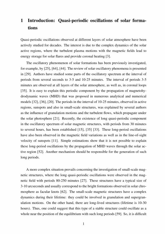
Figure 1. A: the alternating patches represent gas moving down (red) and up

(blue). B: Wave harmonics (l) which penetrate the interior of the Sun. l = 0

- white curve, l = 2 - blue, l = 20 - green, l = 25 - yellow, l = 75 - green.

(Courtesy of J. Christensen-Dalsgaard and Ph. H. Scherrer.). Image source:

https://ase.tufts.edu/cosmos/printimages.asp?id = 25.

Solar oscillatory phenomenon is actively investigated by methods of helioseismol-

ogy. Helioseismology studies the solar interior by analyzing oscillations and waves

propagation on the solar surface. The solar interior is transparent to acoustic (sound)

waves that are excited by turbulent convection below the photosphere and travel with

the speed of sound (Fig.1). The travel times of acoustic waves depend on physical pa-

rameters of the internal layers like temperature, density, velocity of mass flows [30],

[71]. The measurements and the analysis of Doppler velocity established the existence

of 5-minutes oscillations defined as horizontal standing waves propagating on the pho-

tosphere (Fig.2).

2

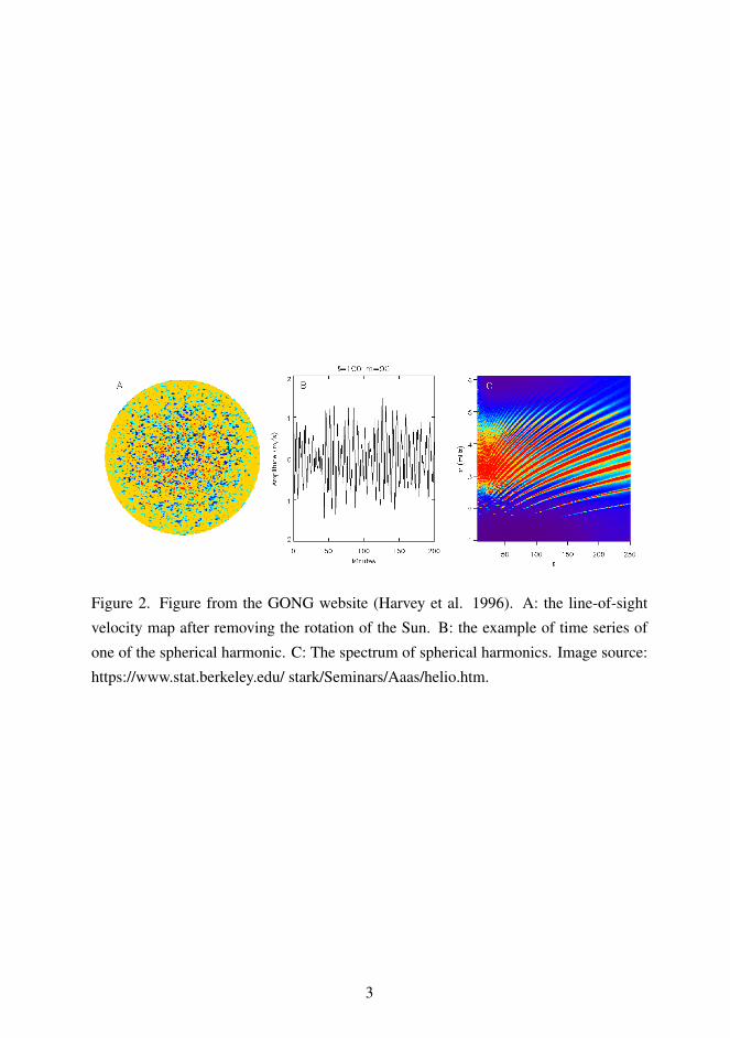
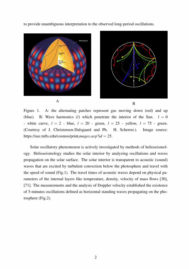
Figure 2. Figure from the GONG website (Harvey et al. 1996). A: the line-of-sight

velocity map after removing the rotation of the Sun. B: the example of time series of

one of the spherical harmonic. C: The spectrum of spherical harmonics. Image source:

https://www.stat.berkeley.edu/ stark/Seminars/Aaas/helio.htm.

3

2 Sunspot: structure

Figure 3. The sunspot visible structure with umbra and penumbra. Image source:

https://www.spaceweatherlive.com/en/help/what-are-sunspots.

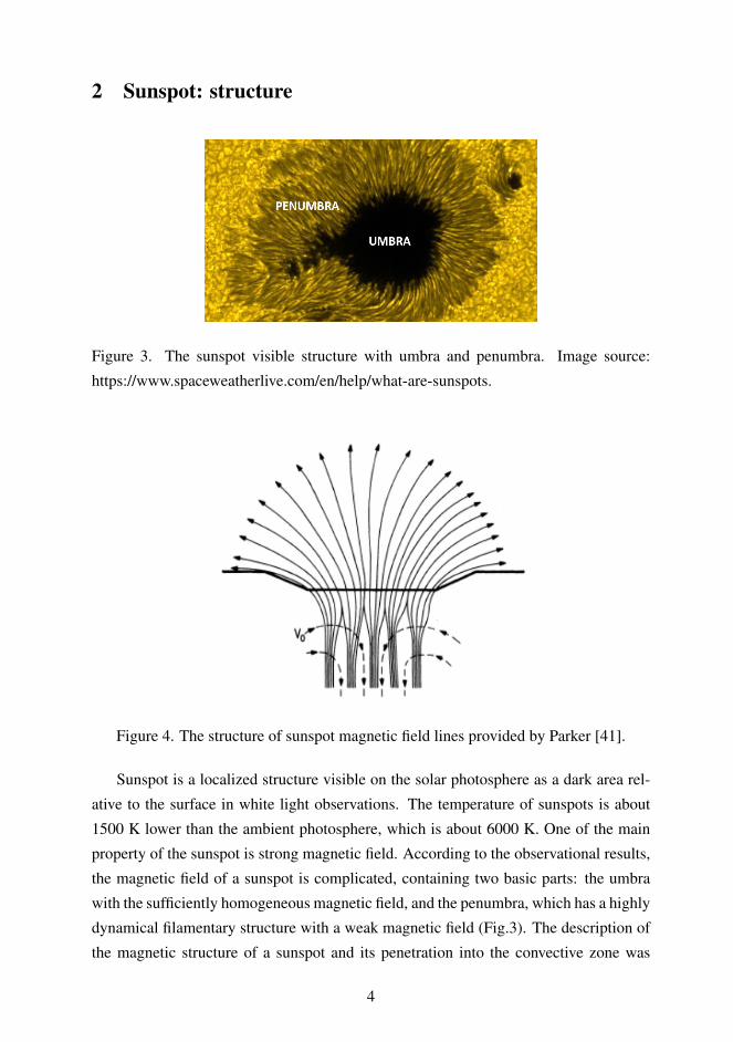
Figure 4. The structure of sunspot magnetic field lines provided by Parker [41].

Sunspot is a localized structure visible on the solar photosphere as a dark area rel-

ative to the surface in white light observations. The temperature of sunspots is about

1500 K lower than the ambient photosphere, which is about 6000 K. One of the main

property of the sunspot is strong magnetic field. According to the observational results,

the magnetic field of a sunspot is complicated, containing two basic parts: the umbra

with the sufficiently homogeneous magnetic field, and the penumbra, which has a highly

dynamical filamentary structure with a weak magnetic field (Fig.3). The description of

the magnetic structure of a sunspot and its penetration into the convective zone was

4

proposed by Parker [41]. According to this model the sunspot is a cluster of magnetic

flux tubes compressed together by the lateral pressure of the environment (Fig.4). A

few hundred kilometers under the photosphere, the magnetic flux tube of the sunspot is

divided into vertical strands. Between these strands weak plasma flows may exist, that

create some extra lateral compression. But the structure of the subsurface layers of a

sunspot was not clearly described in the Parker’s model.

At present, the structure of sunspots is investigated by local helioseismology [71],

[39]. Local helioseismology analyzed frequency and phase shifts of oscillations and

variations in wave travel times in subsurface layers. It requires of high-resolution ob-

servations of solar oscillations [30].

Recent observations of subsurface layers of a sunspot obtained by methods of local

helioseismology established a complex structure of the magnetic field and plasma dy-

namics under the visible sunspot configuration (Fig. 5). It is seen that inside the sunspot

magnetic flux tube the vertical distribution of temperature changes at depths of about

4 Megameters (Mm). Here, a sharp transition takes place between the relatively cold

plasma of a sunspot and the underlying very hot area of plasma, which is overheated to

about 1000 K in comparison to the environment [56].

2.1 Shallow sunspot: formation, stability and long-period oscillations

To understand the nature of the existence of the overheated zone under the sunspot in-

terior, the description of a sunspot formation should be provided. The process of a

sunspot formation is usually described by the emergence of new magnetic flux consist-

ing of magnetic elements of different polarity ([52], Fig. 6). When the vertical magnetic

field Bz exceeds the value of the equipartition field Beq the convective heat transport is

slowed down. The equipartition field is the maximum value of the magnetic field at

which convection is still possible. The equipartition means that the density of the mag-

netic energy is equal to the density of the kinetic energy. We could consider plasma

with density ρ0 and with a speed of convection Vconv. At the level of solar photosphere

[61]: (τ ≈ 1): ρ0 = 2×10−7 g cm−3, Vconv ≈ 1 km s−1, Beq ≈√

4πρ0V 2conv ≈ 200 G.

The value of the magnetic field strength of about 200 G is a threshold value. Stronger

magnetic field suppresses convection, and then the temperature in this area begins to de-

crease [56], [57].

At the top of the overheated region, the overlying flows meet the plasma flows from

the overheated region, which are supported by the convection. The underlying flows

transmit part of their momentum to the overlying streams in the layers of the interaction

5

Figure 5. Sub-photospheric structure of a sunspot obtained by local helioseism-

ogy Colors represent temperature distribution, and arrows represent the flow struc-

ture beneath a sunspot. (Courtesy of the SOHO MDI consortium. SOHO is

a project of international cooperation between ESA and NASA.) Image source:

https://ase.tufts.edu/cosmos/printimages.asp?id = 25.

6

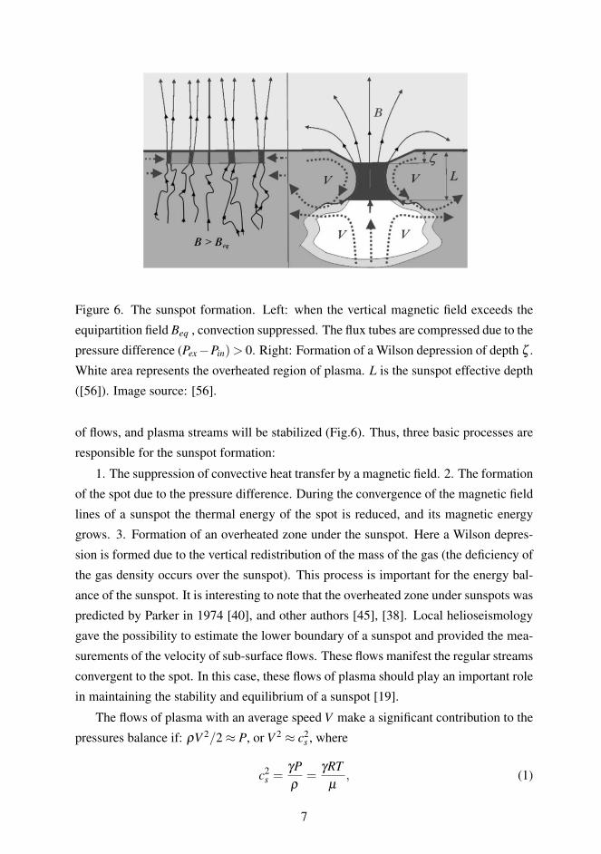
Figure 6. The sunspot formation. Left: when the vertical magnetic field exceeds the

equipartition field Beq , convection suppressed. The flux tubes are compressed due to the

pressure difference (Pex−Pin)> 0. Right: Formation of a Wilson depression of depth ζ .

White area represents the overheated region of plasma. L is the sunspot effective depth

([56]). Image source: [56].

of flows, and plasma streams will be stabilized (Fig.6). Thus, three basic processes are

responsible for the sunspot formation:

1. The suppression of convective heat transfer by a magnetic field. 2. The formation

of the spot due to the pressure difference. During the convergence of the magnetic field

lines of a sunspot the thermal energy of the spot is reduced, and its magnetic energy

grows. 3. Formation of an overheated zone under the sunspot. Here a Wilson depres-

sion is formed due to the vertical redistribution of the mass of the gas (the deficiency of

the gas density occurs over the sunspot). This process is important for the energy bal-

ance of the sunspot. It is interesting to note that the overheated zone under sunspots was

predicted by Parker in 1974 [40], and other authors [45], [38]. Local helioseismology

gave the possibility to estimate the lower boundary of a sunspot and provided the mea-

surements of the velocity of sub-surface flows. These flows manifest the regular streams

convergent to the spot. In this case, these flows of plasma should play an important role

in maintaining the stability and equilibrium of a sunspot [19].

The flows of plasma with an average speed V make a significant contribution to the

pressures balance if: ρV 2/2≈ P, or V 2 ≈ c2s , where

c2s =

γPρ

=γRT

µ, (1)

7

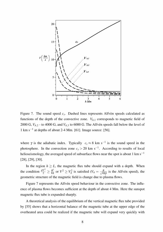
Figure 7. The sound speed cs. Dashed lines represents Alfvèn speeds calculated as

functions of the depth of the convective zone. VA,1 corresponds to magnetic field of

2000 G, VA,2 - to 4000 G, and VA,3 to 6000 G. The Alfvén speeds fall below the level of

1 km s−1 at depths of about 2-4 Mm. [61]. Image source: [56].

where γ is the adiabatic index. Typically cs ≈ 8 km s−1 is the sound speed in the

photosphere. In the convection zone cs > 20 km s−1. According to results of local

helioseismology, the averaged speed of subsurface flows near the spot is about 1 km s−1

[28], [29], [30].

In the region h ≥ L, the magnetic flux tube should expand with a depth. When

the condition ρV 2

2 ≥B2

8πor V 2 ≥ V 2

A is satisfied (VA = B√4πρ

is the Alfvén speed), the

geometric structure of the magnetic field is change due to plasma flows.

Figure 7 represents the Alfvén speed behaviour in the convective zone. The influ-

ence of plasma flows becomes sufficient at the depth of about 4 Mm. Here the sunspot

magnetic flux tube is expanded sharply.

A theoretical analysis of the equilibrium of the vertical magnetic flux tube provided

by [55] shows that a horizontal balance of the magnetic tube at the upper edge of the

overheated area could be realized if the magnetic tube will expand very quickly with

8

depth. Here the sign of the pressure difference Pex−Pin changes at the boundary between

the sunspot and the overheated area that expands the flux tube. Local helioseismology

data show that at a depth of about 4 Mm the pressure difference Pin−Pex is about 1−2× 107 dyn cm−2. The gas pressure difference between the overheated magnetic flux

tube and the environment can be compensated by the sharp horizontal expansion of the

sunspot magnetic tube. So, below the depth of 4 Mm, the sunspot magnetic flux tube

has an irregular structure. Therefore, the level L≈ 4 Mm can be considered as the lower

boundary of the sunspot. It should be noted, that the value L is defined only as the

energetic boundary. The pressure difference Pin−Pex remains negative above the level

h = L when the magnetic field significantly larger than Beq.

The model of the sunspot proposed by Parker [41] describes the sunspot structure

from the visible layers to the boundary L = h. The shallow sunspot model describes

analytically the subsurface levels of a sunspot in accordance to the data obtained with

local helioseismology [54], [55], [56], [57]. The independent successful numerical sim-

ulations have also shown the existence of the overheated area under the sunspot at the

level of about 4 Mm [46].

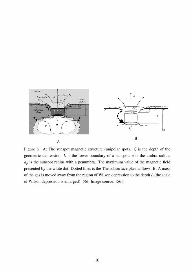
The schematic representation of the magnetic structure of a round unipolar sunspot

(A) and it’s geometrical structure (B) is presented in Fig. 8, in accordance to the "shal-

low sunspot" model. According to the shallow sunspot model, long quasi-periodic os-

cillations of magnetic field and line-of-sight velocities of sunspots are associated with

the slow vertical displacements of a sunspot as a whole.

9

AB

Figure 8. A: The sunspot magnetic structure (unipolar spot). ζ is the depth of the

geometric depression; L is the lower boundary of a sunspot; a is the umbra radius;

ap is the sunspot radius with a penumbra. The maximum value of the magnetic field

presented by the white dot. Dotted lines is the The subsurface plasma flows. B: A mass

of the gas is moved away from the region of Wilson depression to the depth L (the scale

of Wilson depression is enlarged) [56]. Image source: [56].

10

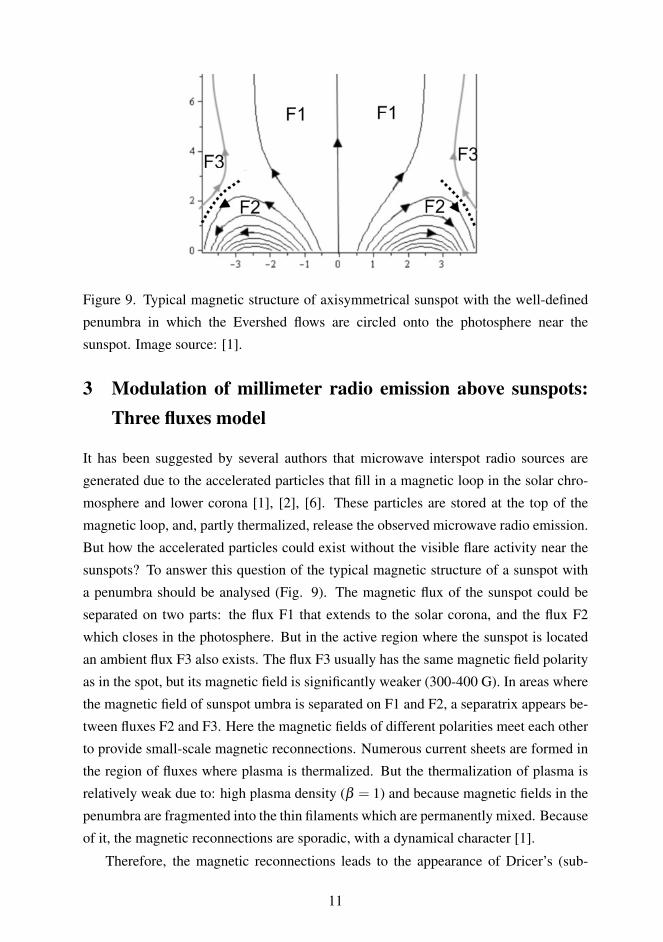
Figure 9. Typical magnetic structure of axisymmetrical sunspot with the well-defined

penumbra in which the Evershed flows are circled onto the photosphere near the

sunspot. Image source: [1].

3 Modulation of millimeter radio emission above sunspots:Three fluxes model

It has been suggested by several authors that microwave interspot radio sources are

generated due to the accelerated particles that fill in a magnetic loop in the solar chro-

mosphere and lower corona [1], [2], [6]. These particles are stored at the top of the

magnetic loop, and, partly thermalized, release the observed microwave radio emission.

But how the accelerated particles could exist without the visible flare activity near the

sunspots? To answer this question of the typical magnetic structure of a sunspot with

a penumbra should be analysed (Fig. 9). The magnetic flux of the sunspot could be

separated on two parts: the flux F1 that extends to the solar corona, and the flux F2

which closes in the photosphere. But in the active region where the sunspot is located

an ambient flux F3 also exists. The flux F3 usually has the same magnetic field polarity

as in the spot, but its magnetic field is significantly weaker (300-400 G). In areas where

the magnetic field of sunspot umbra is separated on F1 and F2, a separatrix appears be-

tween fluxes F2 and F3. Here the magnetic fields of different polarities meet each other

to provide small-scale magnetic reconnections. Numerous current sheets are formed in

the region of fluxes where plasma is thermalized. But the thermalization of plasma is

relatively weak due to: high plasma density (β = 1) and because magnetic fields in the

penumbra are fragmented into the thin filaments which are permanently mixed. Because

of it, the magnetic reconnections are sporadic, with a dynamical character [1].

Therefore, the magnetic reconnections leads to the appearance of Dricer’s (sub-

11

Dricer’s) electric fields that accelerate particles (electrons). They are the physical reason

of the formation of the interspot radio sources [51]. But the real configuration of a

sunspot is usually not ideal. More realistic configuration has the sunspot where a largest

part of the flux F1 is circled onto the other sunspot of different polarity, or onto the area

of the opposite polarity.

Figure 10. Schematic representation of a bipolar sunspot group. In areas where fluxes

F2 and F3 meet each other the small-scale current sheets are generated accelerated par-

ticles. These particles are accumulated in the top of magnetic loops and formed the

interspot radio sources. Image source: [1].

In the low-laying loops the magnetic field is stronger than in the high loops, which

exist at the upper chromosphere and the corona. That leads to the more effective mag-

netic reconnections providing sufficiently energetic particles, which could thermalize

plasma to the X-ray temperatures [66]. In the highest loops the magnetic field is weak

and it could trap a relatively small part of the accelerated particles. But these particles

emit thermal and cyclotron radio emission. In [66] the authors noted that the X-ray

loops near the sunspots are always laying lower than microwave loops. The accelerated

particles are accumulated at the tops of magnetic loops. The formation of a radio source

is due to the partial or full thermalization of these particles. Thermal radio emission is

produced if the thermalization is full, and weak gyrosynchrotron emission could be gen-

erated due to partial thermalization. It should be noticed that millimeter radio sources

are usually characterized as thermal emission sources [23].

In the other case, quasi-periodic and relatively slow variations of the sunspot mag-

netic field are transferred as excitations along the magnetic field lines from the lower-

lying spot to the millimeter radio sources. The time needed for these excitations to

propagate along the magnetic loop from the spot to the source are observed as a time

delay effect [51]. In order to estimate the average velocity of excitation propagation

from the spot to the radio source, one should determine the half-length of the magnetic

loop, at the top of which the radio source is formed. This half-length is l =√

L2 +H2,

where L is the distance from the projection of the radio source position on the photo-

12

sphere to the closest boundary of the sunspot penumbra. We assumed that the height

of the radio source above the photosphere is H = 2 Mm. The length of the projection

of L from the sunspot penumbra boundary to the maximum value of radio emission of

the nearby radio sources was provided by [51] for seven sources. The calculated values

of half-length of the magnetic loops l lay on the interval of 11300-23800 km. The ve-

locity of excitation propagation in the loop along the magnetic field lines was estimated

as V = l/∆Tcorr, where ∆Tcorr is the time-delay observed between oscillations of the

magnetic field of a sunspot and the millimeter radio emission at 37 GHz. Based on the

experiments, we have obtained V = 12.1±1.8 km s−1.

The obtained velocity should probably be associated with the average sound speed

in the magnetic loop. This is related to the fact that millimeter emission of radio sources

is of a purely thermal nature. Therefore, in order for it to be modulated efficiently, the

incoming excitation should alter the plasma temperature-density characteristics in the

source. This process may be completed in no less than the propagation time of acoustic

waves or slow magnetoacoustic waves (with its velocity is equal to the sound speed

cs =√

γRTµ

that propagates along the half-length of the loop). If the obtained velocity

of 12 km s−1 is interpreted as the acoustic wave velocity, the temperature averaged over

the magnetic loop that connects the spot to the radio source equals 11000 K.

Near-spot and interspot radio sources are connected to a spot by the magnetic field

lines. These sources are formed due to thermalization of accelerated particles produced

in small-scale current sheets (Fig.10). Quasi-periodic variations of the magnetic field of

the spot are transferred to the radio source along the magnetic field lines with the speed

of sound. These variations are modulate the slow changes of plasma parameters at radio

source. In other words, the eigen oscillations of the sunspot provided the hydrostatic

rebuilding of the parameters in the millimeter radio source.

13

4 Separated facular knots: long quasi-periodic oscillations

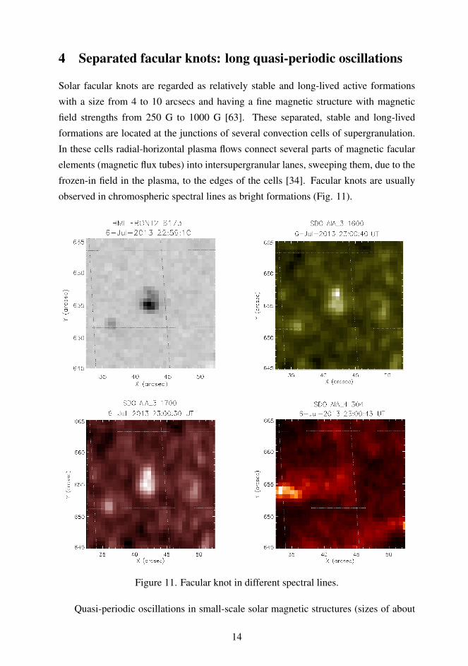
Solar facular knots are regarded as relatively stable and long-lived active formations

with a size from 4 to 10 arcsecs and having a fine magnetic structure with magnetic

field strengths from 250 G to 1000 G [63]. These separated, stable and long-lived

formations are located at the junctions of several convection cells of supergranulation.

In these cells radial-horizontal plasma flows connect several parts of magnetic facular

elements (magnetic flux tubes) into intersupergranular lanes, sweeping them, due to the

frozen-in field in the plasma, to the edges of the cells [34]. Facular knots are usually

observed in chromospheric spectral lines as bright formations (Fig. 11).

Figure 11. Facular knot in different spectral lines.

Quasi-periodic oscillations in small-scale solar magnetic structures (sizes of about

14

4-10 arcsecs), such as faculae and pores, are less studied than sunspots. This is because

the observations with high temporal resolution were unavailable due to the insufficient

temporal resolution of the ground-based instruments. However, using the newest satel-

lite observations with a high spatial and temporal resolutions, we are able to investigate

the oscillatory spectrum of small-scale structures which are observed in different layers

of the solar atmosphere. Recently [4] quasi-periodic oscillations in the facular mag-

netic knots with periods of about 3 minutes were revealed. Additionally, the authors

identified periods of about 5-11 minutes above the facula periphery regions in the 304

Å spectral line. The detected spatial and temporal distribution of the oscillations was

proposed by the authors to be caused by the magnetic field line topology in facular re-

gions. Oscillations with the periods about 5 minutes which depend on the magnetic

field dynamical properties of a facular region were found in [24]. In [16] oscillations

with periods from 3 to 20 minutes in the intensity of two isolated magnetic pores were

detected and interpreted in terms of propagating slow magnetoacoustic sausage waves.

Variations of facular brightness was found to be dependent on the convective motions

in a facular region in [31]. There, the periodicities of about 5 minutes were detected.

The longest periods of oscillations defined in small-scale solar elements do not exceed

30 minutes.

One of the main goals of the study of quasi-periodic oscillations of facular knots is

the construction of an adequate model of a solitary facular knot that satisfies the existing

observations. The construction of such a model primarily requires knowledge of the

magnetic field structure, density, temperature, and pressure distribution in the object. It

is also necessary to take into account the lifetime of the structure, its stability, and its

equilibrium. Therefore, long quasi-periodic oscillations provide information about the

evolution of facular knots during the lifetime.

4.1 Oscillatory modes of facular formations

Previous studies have shown the existence of quasi-periodic variations of the magnetic

field of such small-scale structures, with periods from few minutes to 5-6 h [33]. Vari-

ations (within 25 minutes) were related to the influence of ascending granulation cells

on the structures [21]. The interpretation of longer periods (80-200 min or longer) re-

mains questionable. Quasi-periodic variations of the magnetic field of the facular knots

with periods above 1 hour have been studied by several authors (see, for example: [27],

[62], [58], [60]). In the work [27], such long periods of oscillations were explained

by the influence of supergranulation movements on the structure. But, the lifetime of

15

the granules is about 5-10 minutes. The lifetime of supergranules is about 1.5-2 days.

These lifetimes have a different timescales that do not correspond to the obtained peri-

ods of oscillations in the interval of 80-250 minutes. This oscillatory character was also

explained by the mechanism of vortex separation in the turbulent plasma of the solar

atmosphere [36]. The physical interpretation of long periods of up to 250 minutes could

not be presented in frames of a suggestion of a propagation of MHD waves [21].

4.2 Analytical description of long-period oscillatory modes

We assumed that the magnetic field and the area of the facular knot can vary in time

during the observations. Also the effective mass of the system can be changed. So,

we can consider the facular knot as a system with a time-varying rigidity. Such system

is characterized by a variable character of the response to external disturbances. Let’s

consider the equation of small linear oscillations of the system:

x+2β x+W 2(t)x = 0, (2)

where x is the parameter of the system - the averaged magnetic field strength, β is the

coefficient of the friction, W 2(t) is the effective elasticity of the system. In the case

when W 2 = λ 2q(t) where λ is constant, we can obtain the approximate solution of (2)

(β = 0) by WKB method ([37], formula 14.28):

x(t)≈C1 cos[λ

∫ √qdt]+C2 sin[λ

∫ √qdt]

4√

q. (3)

We postulate the exact solution of (2) in the form:

x(t) = A0 exp[(γ−β )t]cos[ω(t) · t +φ0], (4)

where A0 is the amplitude of the oscillations, γ is the increment/decrement of oscil-

lations, ω(t) is the time varying frequency and φ0 initial phase. Inserting the law of

motion (4) into (2), we obtain:

W 2(t) = (ω + ωt)2− γ2 +β

2, (5)

d(ω + ωt)dt

=−2γ(ω + ωt). (6)

If (ω + ωt)≡ ddt (ωt) = u, we have: u = ω0 exp(−2γt), where ω0 is some characteristic

constant frequency. After the second integration:

16

ωt =ω0

2γexp(−2γt)−φ0. (7)

At t = 0, the phase of oscillations is φ0 =ω02γ

. From equations (5) and (7):

W 2 = ω20 exp(−4γt)− γ

2 +β2 (8)

and the x(t) is:

x(t) = A0 exp[(γ−β )t]cos[

ω0

2γexp(−2γt)+φ0

]. (9)

The function W (t) is a variable function of time, depending mainly on the coefficient

γ: it decreases with time if γ > 0, and grows when γ < 0. Here, W is a complex function

of parameters of the system. It can vary significantly in time. This suggests that during

the observational period, not only the magnetic field and the area of the facular knot can

change. Also the depth of immersion of the facular knot into the photosphere, that is

reflected on its effective mass could vary in time.

17

5 Observations and methods of data processing

5.1 Millimeter radio emission observations

Studies of millimeter radio emission have a special place in present radio astronomy.

This range provides the opportunities for a comprehensive study of the Solar system,

and more distant astronomical objects. The most important parameters of the observed

solar elements, their spatial distribution and fine structure can be obtained by the meth-

ods of millimeter radio observations. Therefore, high-frequency observations are com-

plex both from a technical and methodological point of view. This imposes serious re-

strictions on the technical characteristics of the equipment of the instruments used. The

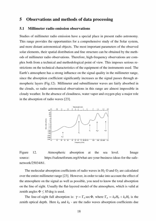
Earth’s atmosphere has a strong influence on the signal quality in the millimeter range,

since the absorption coefficient significantly increases as the signal passes through at-

mospheric layers (Fig.12). Millimeter and submillimeter waves are fairly absorbed in

the clouds, so radio astronomical observations in this range are almost impossible in

cloudy weather. In the absence of cloudiness, water vapor and oxygen play a major role

in the absorption of radio waves [23].

Figure 12. Atmospheric absorption at the sea level. Image

source: https://safenetforum.org/t/what-are-your-business-ideas-for-the-safe-

network/25034/61.

The molecular absorption coefficients of radio waves in H2 O and O2 are calculated

over the entire millimeter range [23]. However, in order to take into account the effect of

the atmosphere on the signal as well as possible, you need to know the total absorption

on the line of sight. Usually the flat-layered model of the atmosphere, which is valid at

zenith angles Φ≤ 85deg is used.

The line-of-sight full absorption is: γ = Γa secΦ, where Γa = kbHb + kkHk is the

zenith optical depth. Here kb and kk - are the radio waves absorption coefficients due

18

to H2O and O2 at the sea level, Hb and Hk the effective path length of the water vapor

and oxygen [8]. For the transparency windows in millimeter range (λ = 8,3.4,2.3,1.4

mm) we could assume kb(h) = exp(−h/Hb), where h is the heigth above the sea level.

The value Hb depends weakly on the air temperature and on h, and could change from

winter to summer in the interval of 1.48−1.56 km [23].

In connection with the above, the requirements for the sensitivity of the receiving

equipment in the millimeter range, to the methods of observation and their primary

processing should be quite high. At present, ground-based radio telescopes and radio

interferometers are used for short-wave observations of astronomical objects [7]. How-

ever, the multitude of tasks facing large systems around the world most often do not

allow concentrating on long-term observations of the same object. Therefore, single

full-turn antennas still play an important role not only as elements of radio interfer-

ometers with very-long bases (VLBI), but also help to solve the tasks of independent

long-term observations of individual radio sources.

5.2 Metsähovi radio telescope

The Metsähovi RT-14 radio-telescope is a Cassegrain-type antenna. The diameter of the

RT-14 is 13.7 m. The telescope could work in range of 2−150 GHz (13.0 cm - 2.0 mm).

The telescope provides two observational methods: solar mapping and the tracking of

the chosen region. At present the 37 GHz receiver is used for solar observations. The

beam size of the antenna is 2.4 arcminutes. The sensitivity of the receiver is 0.2 solar

flux units (s.f.u.). The temporal resolution is 0.1 s [67].

5.3 Helioseismic and Magnetic Imager (SDO/HMI)

Solar Dynamics Observatory (SDO) spacecraft is located in a geosynchronous, inclined

(28.5deg) orbit. Also the spacecraft traces an "eight" spanning 57 degrees in latitude at

an altitude of 36 000 km along the meridian 102deg W. These characteristics provided

a variable component with a period of 12 and 24 hours due to the Doppler effect.

The Helioseismic and Magnetic Imager (HMI) instrument is on-board the SDO. This

instrument provides the measurements of solar magnetic fields and Doppler velocities

every 45 s [47]. The spatial resolution of HMI is 1 arcsecond. A data processing manual

and the description of SDO/HMI is presented in [48], [49], [9], [68]. Full-disk solar

maps of the line-of-sight magnetic field could be obtained by using the Joint Science

Operation Centre (JSOC) HMI-AIA Science Data Processing.

19

5.4 Methods of data processing

5.4.1 Wavelet transform

The Wavelet analysis is the most popular method for the investigation of the distribution

of periods of quasi-periodic oscillations in time in various signals. In other words, it

enables to study the signal behaviour both in the time and in the frequency domain.

Here the signal analyzed by "mother" function (Ψ), as well as, by the changing of the

time delay (τ) and the scale (s). The continuous Wavelet transform is defined as [65]:

W Ψx (τ,s) =

1√|s|

∫ +∞

−∞

x(t)Ψ∗(

t− τ

s

)dt, (10)

where the (*) indicates the complex conjugate. Mostly the Morlet wavelet is used as a

mother function to analyse non-stationary signals. This is because it has the minimum

value of the square in frequency-time resolution, i.e. the maximum frequency resolution

[10]. The Morlet function is defined as:

Ψ(t) = π1/4eiω0te−t2/2, (11)

where ω0 is the dimensionless frequency [13].

5.4.2 Empirical Mode Decomposition (EMD)

The empirical mode decomposition (EMD) is iteratively decompose the signal into nat-

ural harmonics by using a shift-factor (local time-scale of the real signal) [18]. EMD

method does not use the harmonic functions (as sine, cosine, or wavelets) as a basis.

Due to its adaptive nature, EMD is suitable for analysing nonlinear variations [18].

Application of the EMD technique to the average magnetic field time-series allows

us to extract several intrinsic empirical modes from the signal. We can estimate periods

of the empirical modes as P = 2N/n. Here N is the total length of the analyzed signal;

n is the number of extrema in a mode. Also, EMD may indicate a random nature

of empirical modes [14]. Writing the power spectral density S as a function of the

frequency f as S = 1/ f α [70], [26], we are able to compare the modes with the white

and coloured noises. Recently it was shown [26] that the energy E of the intrinsic modes

obtained from synthetic coloured noise time-series is connected with the mean period

of the modes.

20

6 Results (summary of the publications)

All articles included in this thesis are dedicated to the investigation of long quasi-

periodic oscillations of observed physical parameters of sunspots and small-scale mag-

netic structures with periods more than 30 minutes.

6.1 Long quasi-periodic oscillations of sunspots and nearby magnetic struc-tures

This article was aimed to investigate the long quasi-periodic oscillations of the averaged

value of the line-of-sight component of the sunspot magnetic field. We analysed five ac-

tive regions with sunspots using data obtained from SDO/HMI and from the Metsähovi

RT-14 radio-telescope at 37 GHz frequency. The periods in the interval of 200-400

minutes were found in the time-series of the magnetic field and radio emission. The

analysis of time-series of the magnetic field and the radio emission showed that the os-

cillations with periods of 200-400 minutes occur in phase, but the radio emission vari-

ations are delayed relative to the magnetic field variations. Time lags of 15-18 minutes

were found. We proposed the modulation mechanism of radio emission at high levels

is the magneto-hydrostatic rebuilding of radio sources caused by slow time-variation of

the sunspot magnetic field. The interpretation of observed long periods was also given

with the "shallow sunspot" model, which represents the sunspot as a stable, isolated

magnetic structure, which could oscillate as a whole near the position of equilibrium.

6.2 Artifacts of SDO/HMI data and long-period oscillations of sunspots

In this article the periodic artifacts with periods of 12 and 24 hours found in SDO/HMI

data series were investigated. These artifacts appeared in long time-series during the

analysis of quasi-periodic variations of sunspots. It was found that these artifacts are

well detected in the regions of weak magnetic fields. The artifitial harmonics do not

significantly affect to the long-period oscillations of sunspots if the maximum value of

the magnetic field of the spot is less than 2000 G. If the magnetic field is higher than

2000 G, the amplitude of artifacts grows and become significant.

21

6.3 Time delay effect between long quasi-periodic oscillations of 37 GHzradio sources and the magnetic field of the nearest sunspots

In this article we continued the detailed investigations of the time-delay effect observed

between the variations of the magnetic field and the radio intensity at 37 GHz. For seven

active regions several parameters were found: periods of oscillations of the magnetic

field and radio emission; time-delays obtained with the cross-correlation analysis, time-

delays obtained as the time propagation of the acoustic disturbances from the sunspot

to the radio source for temperatures of 10000 K, 11000 K and 12000 K; the half-length

of the magnetic loop where the radio sources are originated. All time-delays were very

close. The interpretation of these time-delays and the description of the relation between

sunspots and radio sources observed at 37 GHz was given with the "free-fluxes" model.

6.4 Long-period quasi-periodic oscillations of a small-scale magnetic struc-ture on the Sun

This article represents the study of long-period non-linear variations of the magnetic

field of the solar small-scale magnetic structure. To obtain the period of variations the

Empirical Mode Decomposition method was used. The obtained modes were tested

with the synthetic noises (white, pink and red), and the significant mode with the period

of 80-260 minutes was found. This mode showed non-linear character with the growing

amplitude and period. We interpreted such oscillatory phenomenon in terms of the

vortex shedding appearing during the emergence of the magnetic flux of the structure.

Such long period oscillations could be induced by the dynamical interaction of small-

scale magnetic structures with the supergranula cells.

6.5 Long-term oscillations of sunspots and a special class of artifacts inSOHO/MDI and SDO/HMI data

A special class of artifacts named pixel-to-pixel (p2p) were described in this article.

These artifacts appear when we track the pixel on the CCD matrix, i.e. when the image

moves along the pixel matrix. We found the period of p2p artifact for SDO data of

about 3 minutes. The results of the detailed analysis of two types of p2p artifact show

that the integral parameters of the source observed with the CCD matrix should be used

for studying of quasi-periodic oscillations of source parameters instead of the maximum

values of the source obtained from the one pixel. Artifact neutralization is possible only

if we analyse the source-average values of physical parameters. Several tests confirmed

22

the existing of oscillations of physical parameters of sunspots, independent of the arti-

facts. For example, the simultaneous analysis of sunspot magnetic field and ultraviolet

intensity of its umbra showed the same periods of oscillations.

6.6 Eigen oscillations of facular knots

Long-period non-linear oscillations of the magnetic field of small-scale magnetic struc-

tures as facular knots were analysed in this article. Three regimes of oscillations were

found: the increasing of the amplitude and the period; the decreasing of the amplitude

and the period; and the growth and decrease of the amplitude and period alternate one

another. The theoretical interpretation of these regimes of oscillations of facular knots

was proposed. We suggested the facular knot as a system with the time-varying rigid-

ity. The oscillations of the system with the time-varying rigidity were estimated. The

comparison of the observed and estimated oscillatory modes shown good agreement. It

was shown that even if objects retain their structural identity, their physical parameters

can vary significantly. The variations of the parameters could change the response of

the system to the external disturbances that lead to the changing of the character of ob-

served oscillations. Obviously, the rigidity of the facular knots is a complex function of

physical parameters of the system. It vary in time significantly during the observations.

Also, the depth of immersion of the facular knot into the photosphere, which is directly

reflected on its effective mass, could vary in time.

7 Conclusions

The thesis aimed to provide the analysis and the interpretation of long quasi-periodic

oscillations of the magnetic field of sunspots and the penetration of these oscillations

into the high levels of solar atmosphere, which was observed at millimeter radio waves.

Also, we analyzed the long quasi-periodicity at small-scale magnetic structures like

facular knots and pores. We provided the interpretation of long-period oscillations of

sunspots as well as the long-periodical component observed in the oscillatory spectrum

of facular knots in frames of model of a shallow sunspot (periods from 60 minutes and

more).

So-called "three-fluxes model" is the additional part of the shallow sunspot model. This

model explains the formation and the long-period oscillations of radio sources, which

lay in the solar chromosphere, nearby spots.

Extrapolating the shallow sunspot model to the facular knots, we met some difficulties,

23

like the incomplete knowledge of a number of physical parameters (mass of the object,

lower boundary) that should be included in the model. Because of that, firstly, we care-

fully analyzed the dynamics of facular knots based on the observations of the magnetic

field variations, and the intensity variations at UV spectral lines. We obtained three

types of non-linear long-period oscillatory modes with periods from 25 to 250 minutes:

1. The period and the amplitude increase with time; 2. The period and amplitude de-

crease with time; 3. The changing regime of the growing and the decreasing of the

period and the amplitude, as the beats, where the period of oscillations does not depend

on the amplitude. All observed modes were interpreted in terms of oscillations of the

system with the time-varying rigidity [59]. The second step is to estimate theoretically

the values of periods of oscillations comparable with the observed long periods. Using

the estimations of characteristic frequency of oscillations of a facular knot provided by

[59], and based on the assumption that the lower boundary of a facular knot L is about 1

- 2 Mm, we obtained the period T = 150 minutes. This value is in the good agreement

with the observed periods.

8 Outlook

Future work will directed to the statistical investigations of facular knots and pores.

There are still several questions concerning the evolution and the physical parameters of

these small-scale magnetic structures: 1. what is the typical lifetime of facular knots? 2.

how these objects distributed on the Sun during the solar cycles? 3. what is the structural

evolution of these objects? 4. how the intensity of facular knots is changes with the

height? 5. if these objects are long-lived, what factors provide its stability? There is

no adequate theoretical model of a separated facular knot with a lifetime is more than

5 hours. New analytical and numerical model of a facular knot will be proposed based

on the observational results of the dynamical properties of these objects, and on the

theoretical suggestions which was described in the thesis.

One of the important question which will be investigated in our future work is the new

theoretical model of the dissipation of a sunspot. This process has a complex character

when the system of a sunspot loose its stability and the equilibrium. New theoretical

interpretation of the sunspot dissipation process will give the possibility to describe the

sunspot evolution in more detail.

24

References

[1] Bakunina, I.A., Abramov-maximov, V.E., Nakariakov, V.M., Lesovoy, S.V.,

Soloviev, A.A., Tikhomirov, Y.V., Melnikov, V.F., Shibasaki, K., Nagovitsyn, Y.A.,

Averina, E.L. 2013, PASJ, 65, 13.

[2] Bakunina, I.A., Melnikov, V.F., Solov’ev, A.A., Abramov-Maximov, V.E. 2014,

Sol. Phys. 290, 37

[3] Bogdan, T. 2000 Sunspot Oscillations and Seismology, Encyclopedia of Astron-

omy and Astrophysics, Edited by Paul Murdin, article id. 2299. Bristol: Institute of

Physics Publishing, 2001.

[4] Chelpanov, A. A., Kobanov, N. I., & Kolobov, D. Y. 2015, Astronomy Reports, 59,

968

[5] Cheung, M. C. M., Moreno-Insertis, F., & Schüssler, M. 2006, A&A, 451, 303

[6] Chorley, N., Hnat, B., Nakariakov, V.M., Inglis, A.R., Bakunina, I.A. 2010, Astron.

Astrophys. 513, 27

[7] Christiansen U., Hogbom I. 1972, Radiotelescopes, Mir, 255

[8] Chukin V.V. 2004, Monography, RGGMU, 107

[9] Couvidat, S., Schou, J, Shine, R. A., et al. 2012, Sol. Phys., 275, 285

[10] Daubechies, I. 1992, Ten lectures on wavelets, Society for industrial and applied

mathematics

[11] Efremov, V.I., Parfinenko, L.D., Solov’ev, A.A. 2010, Sol. Phys. 267, 279

[12] Efremov, V. I., Parfinenko, L, D., Solov’ev, A. A. 2012, Geomagnetism and Aeron-

omy, 52, 1055

[13] Farge, M., 1992: Wavelet transforms and their applications to turbulence. Annu.

Rev. Fluid Mech., 24, 395–457.

[14] Flandrin, P., Rilling, G., & Goncalves, P. 2004, IEEE Signal Processing Letters,

11, 112

[15] Foullon, C., Verwichte, E., & Nakariakov, V. M. 2009, ApJ, 700, 1658

25

[16] Freij, N., Dorotovic, I., Morton, R. J., et al. 2016, ApJ, 817, 44

[17] Gelfreikh, G. B., Nagovitsyn, Y. A., & Nagovitsyna, E. Y. 2006, PASJ, 58, 29

[18] Huang, N. E., Shen, Z., Long, S. R., Wu, M. C., Shih, H. H., Zheng, Q., Yen, N.

C., Tung, C. C., and Liu, H. H., 1998, Proc. Roy. Soc. Lond. A, 454, 903

[19] Hulburt, N.E., Rucklidge, A.M. 2000, Mon. Not. R. Astron. Soc. 314, 793

[20] Jelinek, P.; Karlický, M.; Van Doorsselaere, T.; Bárta, M. 2017, ApJ, 847, 98J

[21] Jess, D.B., Morton, R.J., Verth, G, Fedun, V., Grant, S.D.T., Giagkiozis, I. 2015,

Sp.Sc.Rev., 190, 1-4, 103

[22] Jess, D.B., Verth, G. 2016, Washington DC American Geophysical Union Geo-

physical Monograph Series 216, 449, 1502.06960

[23] Kislyakov A. G. 1970, Physics-Uspekhi, 101, 4, 607

[24] Kobanov, N., Kolobov, D., & Chelpanov, A. 2015, Sol. Phys., 290, 363

[25] Kobrin, M. M., Pakhomov, V. V., & Prokofeva, N. A. 1976, Sol. Phys., 50, 113

[26] Kolotkov, D. Y., Anfinogentov, S. A., & Nakariakov, V. M. 2016, A&A, 592, A153

[27] Kolotkov, D.Y., Smirnova, V.V., Strekalova, P.V., Riehokainen, A., and Nakari-

akov, V.M., 2017, A&A 598, L2.

[28] Kosovichev, A. G. 2006, Adv. Space Res., 38, 876

[29] Kosovichev, A.G. 2009, Space Sci. Rev. 144, 175

[30] Kosovichev, A.G. 2012, Sol. Phys. 279, 323

[31] Kostik, R. & Khomenko, E. 2016, A&A, 589, A6

[32] Kshevetskii, S.P., Solov’ev, A.A. 2008 Astron. Rep. 52, 772

[33] Martínez González, M.J., Asensio Ramos, A., Manso Sainz, R., et al., 2011, As-

tron. J. Lett., 730, 2, L37

[34] Mehltretter J.P. 1974, Sol. Phys. 38, 43

[35] Nakariakov, V.M., Stepanov, A.V.A.: In: Klein, K.-L., MacKinnon, A.L. (eds.)

2007, Lecture Notes in Physics, vol. 725, p. 221

26

[36] Nakariakov, V.M., Aschwanden, M.J., & van Doorsselaere T. 2009, A&A, 502,

661

[37] Nayfeh, Ali H. 1981, A Wiley-Interscience Publication, New York: Wiley

[38] Obridko, V.N. 1985, Sunspots and Complexes of Activity. Nauka, Moscow, pp.

255

[39] Parchevsky, K. V., & Kosovichev, A. G. 2009, ApJ, 694, 573

[40] Parker, E.N. 1974, Sol. Phys. 36, 249

[41] Parker, E.N. 1979, Astrophys. J. 230, 905

[42] Parker, E.N. 1979, Cosmical Magnetic Fields. Part I. Claredon Press, Oxford, pp.

608

[43] Parker, E.N. 2008, Space Sci. Rev. 144, 15

[44] Pevtsov, A.A., Berteo, L., Tlatov, A.G., Kilcik, A., Nagovitsyn, Yu.A., Cliver,

E.W. 2014, Sol. Phys. 289, 593

[45] Ponomarenko, Y.B. 1972, Sov. Astron. 16, 116

[46] Rempel, M. 2012, Astrophys. J. 750, 62

[47] Scherrer, P. H., Schou, J., Bush, R. I., et al. 2012, Sol. Phys., 275, 207

[48] Schou, J., & Larson, T. P. 2011, SPD Meeting 42, 16.05, BAAS, 43

[49] Schou, J., Scherrer, P. H., Bush, R. I., et al. 2012, Sol. Phys., 275, 229

[50] Smirnova, V., Riehokainen, A., Solov’ev, A. A., & Kallunki, J. 2015, AP&SS,

357, 2, 149

[51] Smirnova, V.V., Riehokainen, A., Ryzhov, V., Zhiltsov, A., & Kallunki, J. 2011,

A&A, 534, A137

[52] Smirnova, V., Riehokainen, A., Solov’ev, A., Kallunki, J., Zhiltsov, A., Ryzhov,

V. 2013, A&A, 552, 23

[53] Smirnova, V., Efremov, V.I., Parfinenko, L.D., Riehokainen, A., Solov’ev, A.A.

2013, A&A, 554, A121, 7

27

[54] Solov’ev, A. A., & Kirichek, E. A. 2008, Astrophys. Bull., 63, 169

[55] Solov’ev, A. A., & Kirichek, E. A. 2009, Astron. Rep., 53, 675

[56] Solov’ev, A., Kirichek, E. 2014, Astrophys. Space Sci. 352, 23

[57] Solov’ev, A.A., Kirichek, E.A. 2015, Astron. Lett. 41, 211

[58] Solov’ev, A.A., Kirichek, E.A., Efremov, V.I. 2017, Geomagnetism and Aeron-

omy 57, 1101

[59] Solov’ev, A. A., & Kirichek, E. A. 2019, MNRAS, 482, 4, 5290

[60] Solov’ev, A. A., Strekalova P.V., Smirnova V.V., Riehokainen A. 2019, Ap&SS,

364, 29S

[61] Stix, M. 2004, The sun: an introduction, 2nd ed., by Michael Stix. Astronomy and

astrophysics library, Berlin: Springer, ISBN: 3540207414

[62] Strekalova, P.V., Nagovitsyn, Yu.A., Riehokainen, A., and Smirnova, V.V., 2016,

Geomagn. Aeron. (Engl. Transl.), 56, 8, 1052.

[63] P. V. Strekalova, Yu. A. Nagovitsyn, and V. V. Smirnova, 2018, Geomagn. Aeron.

(Engl. Transl.), 58, 7, 893.

[64] Thomas, J. H., Cram, L. E., & Nye, A. H. 1984, ApJ, 285, 368

[65] Torrence, C., & Compo, G. P. 1998, Bull. Am. Meteorol. Soc., 79, 61

[66] Tun, S.D., Gary, D.E., Georgoulis, M.K. 2011, ApJ, 728, 1, 1, 16

[67] Urpo, S. 1982, Observing methods for the millimeter wave radio telescope at the

Metsaehovi Radio Research Station and observations of the Sun and extragalactic

sources. Ph.D. Thesis. Helsinki University of Technology, Espoo, Finland

[68] Wachter, R., Schou, J., Rabello-Soares, M. C., et al. 2012, Sol. Phys., 275, 261

[69] Wilhelm, K. 2009, Landolt Börnstein, 4115

[70] Wu, Z. & Huang, N. E. 2004, Proceedings of the Royal Society of London Series

A, 460, 1597

[71] Zhao, J., Kosovichev, A. G., & Duvall, Jr., T. L. 2001, ApJ, 557, 384

28