LONG SHORT-TERM MEMORYTechnical Report FKI-207-95, Version 3.0Sepp HochreiterFakult�at f�ur InformatikTechnische Universit�at M�unchen80290 M�unchen, Germanyhochreit@informatik.tu-muenchen.dehttp://www7.informatik.tu-muenchen.de/~hochreit J�urgen SchmidhuberIDSIACorso Elvezia 366900 Lugano, Switzerlandjuergen@idsia.chhttp://www.idsia.ch/~juergenRevised December 1996AbstractLearning to store information over extended time intervals via recurrent backpropagationtakes a very long time, mostly due to insu�cient, decaying error back ow. We brie y reviewHochreiter's 1991 analysis of this problem, then address it by introducing a novel, e�cientmethod called \Long Short-Term Memory" (LSTM). LSTM can learn to bridge time lagsin excess of 1000 steps by enforcing constant error ow through \constant error carrousels"within special units. Multiplicative gate units learn to open and close access to the constanterror ow. LSTM's update complexity per time step is O(W ), where W is the number ofweights. In experimental comparisons with RTRL, BPTT, Recurrent Cascade-Correlation,Elman nets, and Neural Sequence Chunking, LSTM leads to many more successful runs, andlearns much faster. LSTM also solves complex long time lag tasks that have never been solvedby previous recurrent network algorithms. It works with local, distributed, real-valued, andnoisy pattern representations.1 INTRODUCTIONRecurrent networks can in principle use their feedback connections to store representations ofrecent input events in form of activations (\short-term memory", as opposed to \long-term mem-ory" embodied by slowly changing weights). This is potentially signi�cant for many applications,including speech processing, non-Markovian control, and music composition (e.g., Mozer 1992).The most widely used algorithms for learning what to put in short-term memory, however, taketoo much time or don't work well at all, especially when minimal time lags between inputs andcorresponding teacher signals are long.With conventional \Back-Propagation Through Time" (BPTT, e.g., Williams and Zipser 1992)or \Real-Time Recurrent Learning" (RTRL, e.g., Robinson and Fallside 1987), error signals \ ow-ing backwards in time" tend to either (1) blow up or (2) vanish: the temporal evolution of thebackpropagated error exponentially depends on the size of the weights. Case (1) may lead tooscillating weights, while in case (2) learning to bridge long time lags takes a prohibitive amountof time, or does not work at all.This paper presents \Long Short-Term Memory" (LSTM), a novel recurrent network archi-tecture in conjunction with an appropriate gradient-based learning algorithm. The combinationof both is designed to overcome these error back- ow problems. Unlike Schmidhuber's (1992b)chunking systems (which work well if input sequences contain local regularities that make thempartly predictable), LSTM can learn to bridge time intervals in excess of 1000 steps even in noisy,1

highly unpredictable environments, without loss of short time lag capabilities. The LSTM ar-chitecture achieves this by enforcing constant (thus neither exploding nor vanishing) error owthrough internal states of special units | a feature which also makes the method fast.Outline of paper. Section 2 begins with an outline of the detailed analysis of vanishing errorsdue to Hochreiter (1991). It will then introduce a naive approach to constant error backprop fordidactic purposes, and highlight its problems concerning information storage and retrieval. Theseproblems will lead to the LSTM architecture as described in Section 3. Section 4 will presentnumerous experiments and comparisons with competing methods. LSTM outperforms them, andalso learns to solve complex tasks no other recurrent net algorithm has solved. Section 5 willbrie y review previous work. Section 6 will discuss certain limitations and advantages of LSTM.The appendix contains a detailed description of the algorithm (A.1), and explicit formulae forerror ow (A.2).2 CONSTANT ERROR BACKPROP2.1 EXPONENTIALLY DECAYING ERRORConventional BPTT (e.g. Williams and Zipser 1992). Output unit k's target at time t isdenoted by dk(t). Using mean squared error, k's error signal is#k(t) = f 0k(netk(t))(dk(t)� yk(t));where yi(t) = fi(neti(t))is the activation of a non-input unit i with di�erentiable activation function fi,neti(t) =Xj wijyj(t � 1)is unit i's current net input, and wij is the weight on the connection from unit j to i. Somenon-output unit j's backpropagated error signal is#j(t) = f 0j(netj(t))Xi wij#i(t+ 1):The corresponding contribution to wjl's total weight update is �#j(t)yl(t � 1), where � is thelearning rate, and l stands for an arbitrary unit connected to unit j.Outline of Hochreiter's analysis (1991, page 19-21). Suppose we have a fully connectednet whose non-input unit indices range from 1 to n. The error occurring at an arbitrary unit u attime step t is propagated \back into time" for q time steps, to an arbitrary unit v. This will scalethe error by the following factor:@#v(t� q)@#u(t) = ( f 0v(netv(t� 1))wuv q = 1f 0v(netv(t � q))Pnl=1 @#l(t�q+1)@#u(t) wlv q > 1 : (1)With lq = v and l0 = u, we obtain:@#v(t � q)@#u(t) = nXl1=1 : : : nXlq�1=1 qYm=1 f 0lm (netlm (t�m))wlm lm�1 (2)(proof by induction). The sum of the nq�1 terms Qqm=1 f 0lm (netlm (t�m))wlmlm�1 determines thetotal error back ow (note that since the summation terms may have di�erent signs, increasingthe number of units n does not necessarily increase error ow).2

Intuitive explanation of equation (2). Ifjf 0lm (netlm (t �m))wlm lm�1 j > 1:0for all m (as can happen, e.g., with linear flm ) then the largest product increases exponentiallywith q. That is, the error blows up, and con icting error signals arriving at unit v can lead tooscillating weights and unstable learning. On the other hand, ifjf 0lm (netlm (t �m))wlm lm�1 j < 1:0for all m, then the largest product decreases exponentially with q. That is, the error vanishes, andnothing can be learned in acceptable time.If flm is the logistic sigmoid function, then the maximal value of f 0lm is 0.25. If ylm�1 is constantand not equal to zero, then jf 0lm (netlm )wlmlm�1 j takes on maximal values wherewlmlm�1 = 1ylm�1 coth(12netlm );goes to zero for jwlmlm�1 j ! 1, and is less than 1:0 for jwlmlm�1 j < 4:0 (e.g., if the absolute max-imal weight value wmax is smaller than 4.0). Hence with conventional logistic sigmoid activationfunctions, the error ow tends to vanish as long as the weights have absolute values below 4.0,especially in the beginning of the training phase. In general the use of larger initial weights won'thelp though | as seen above, for jwlmlm�1 j ! 1 the relevant derivative goes to zero \faster"than the absolute weight can grow (also, some weights will have to change their signs by crossingzero). Likewise, increasing the learning rate does not help either | it won't change the ratio oflong-range error ow and short-range error ow. BPTT is too sensitive to recent distractions. (Avery similar, more recent analysis was presented by Bengio et al. 1994).Weak upper bound for scaling factor. The following, slightly extended vanishing erroranalysis also takes n, the number of units, into account. For q > 1, formula (2) can be rewrittenas (WuT )T F 0(t � 1) q�1Ym=2 (WF 0(t �m)) Wv f 0v(netv(t� q));where the weight matrixW is de�ned by [W ]ij := wij, v's outgoing weight vector Wv is de�ned by[Wv]i := [W ]iv = wiv, u's incomingweight vectorWuT is de�ned by [WuT ]i := [W ]ui = wui, and form = 1; : : : ; q, F 0(t�m) is the diagonal matrix of �rst order derivatives de�ned as: [F 0(t�m)]ij := 0if i 6= j, and [F 0(t � m)]ij := f 0i (neti(t � m)) otherwise. Here T is the transposition operator,[A]ij is the element in the i-th column and j-th row of matrix A, and [x]i is the i-th componentof vector x.Using a matrix norm k : kA compatible with vector norm k : kx, we de�nef 0max := maxm=1;:::;qfk F 0(t�m) kAg:For maxi=1;:::;nfjxijg � k x kx we get jxTyj � n k x kx k y kx : Sincejf 0v(netv(t� q))j � k F 0(t� q) kA � f 0max;we obtain the following inequality:j @#v(t� q)@#u(t) j � n (f 0max)q kWv kx kWuT kx kW kq�2A � n (f 0max kW kA)q :This inequality results fromkWv kx = kWev kx � k W kA k ev kx � k W kAand k WuT kx = k euW kx � kW kA k eu kx � kW kA;3

where ek is the unit vector whose components are 0 except for the k-th component, which is 1.Note that this is a weak, extreme case upper bound | it will be reached only if all k F 0(t�m) kAtake on maximal values, and if the contributions of all paths across which error ows back fromunit u to unit v have the same sign. Large k W kA, however, typically result in small values ofk F 0(t �m) kA, as con�rmed by experiments (see, e.g., Hochreiter 1991).For example, with norms k W kA := maxrXs jwrsjand k x kx:= maxrjxrj;we have f 0max = 0:25 for the logistic sigmoid. We observe that ifjwijj � wmax < 4:0n 8i; j;then k W kA � nwmax < 4:0 will result in exponential decay | by setting � := �nwmax4:0 � < 1:0,we obtain j @#v(t� q)@#u(t) j � n (� )q :We refer to Hochreiter's 1991 thesis for additional details.2.2 CONSTANT ERROR FLOW: NAIVE APPROACHA single unit. To avoid vanishing error signals, how can we achieve constant error ow througha single unit j with a single connection to itself? According to the rules above, at time t, j's localerror back ow is #j(t) = f 0j(netj(t))#j(t + 1)wjj. To enforce constant error ow through j, werequire f 0j(netj(t))wjj = 1:0:Note the similarity to Mozer's �xed time constant system (1992) | a time constant of 1:0 isappropriate for potentially in�nite time lags1.The constant error carrousel. Integrating the di�erential equation above, we obtainfj(netj(t)) = netj(t)wjj for arbitrary netj(t). This means: fj has to be linear, and unit j's acti-vation has to remain constant:yj(t + 1) = fj(netj(t+ 1)) = fj(wjjyj(t)) = yj(t):In the experiments, this will be ensured by using the identity function fj : fj(x) = x; 8x, and bysetting wjj = 1:0. We refer to this as the constant error carrousel (CEC). CEC will be LSTM'scentral feature (see section 3).Of course unit j will not only be connected to itself but also to other units. This invokes twoobvious, related problems (also inherent in all other gradient-based approaches):1. Input weight con ict: for simplicity, let us focus on a single additional input weight wji.Assume that the total error can be reduced by switching on unit j in response to a certain input,and keeping it active for a long time (until it helps to compute a desired output). Provided i is non-zero, since the same incoming weight has to be used for both storing certain inputs and ignoringothers, wji will often receive con icting weight update signals during this time (recall that j islinear): these signals will attempt to make wji participate in (1) storing the input (by switchingon j) and (2) protecting the input (by preventing j from being switched o� by irrelevant laterinputs). This con ict makes learning di�cult, and calls for a more context-sensitive mechanismfor controlling \write operations" through input weights.2. Output weight con ict: assume j is switched on and currently stores some previousinput. For simplicity, let us focus on a single additional outgoing weight wkj. The same wkj has1We do not use the expression \time constant" in the di�erential sense, as, e.g., Pearlmutter 1995.4

to be used for both retrieving j's content at certain times and preventing j from disturbing kat other times. As long as unit j is non-zero, wkj will attract con icting weight update signalsgenerated during sequence processing: these signals will attempt to make wkj participate in (1)accessing the information stored in j and | at di�erent times | (2) protecting unit k from beingperturbed by j. For instance, with many tasks there are certain \short time lag errors" that can bereduced in early training stages. However, at later training stages j may suddenly start to causeavoidable errors in situations that already seemed under control by attempting to participate inreducing more di�cult \long time lag errors". Again, this con ict makes learning di�cult, andcalls for a more context-sensitive mechanism for controlling \read operations" through outputweights.Of course, input and output weight con icts are not speci�c for long time lags, but occur forshort time lags as well. Their e�ects, however, become particularly pronounced in the long timelag case: as the time lag increases, (1) stored information must be protected against perturbationfor longer and longer periods, and | especially in advanced stages of learning | (2) more andmore already correct outputs also require protection against perturbation.Due to the problems above the naive approach does not work well except in case of certainsimple problems involving local input/output representations and non-repeating input patterns(see Hochreiter 1991 and Silva et al. 1996). The next section shows how to do it right.3 LONG SHORT-TERM MEMORYMemory cells and gate units. To construct an architecture that allows for constant error owthrough special, self-connected units without the disadvantages of the naive approach, we extendthe constant error carrousel CEC embodied by the self-connected, linear unit j from Section 2.2by introducing additional features. A multiplicative input gate unit is introduced to protect thememory contents stored in j from perturbation by irrelevant inputs. Likewise, a multiplicativeoutput gate unit is introduced which protects other units from perturbation by currently irrelevantmemory contents stored in j.The resulting, more complex unit is called a memory cell (see Figure 1). The j-th memory cellis denoted cj . Each memory cell is built around a central linear unit with a �xed self-connection(the CEC). In addition to netcj , cj gets input from a multiplicative unit outj (the \output gate"),and from another multiplicative unit inj (the \input gate"). inj 's activation at time t is denotedby yinj (t), outj's by youtj (t). We haveyoutj (t) = foutj (netoutj (t)); yinj (t) = finj (netinj (t));where netoutj (t) =Xu woutjuyu(t� 1);and netinj (t) =Xu winjuyu(t� 1):We also have netcj (t) =Xu wcjuyu(t � 1):The summation indices u may stand for input units, gate units, memory cells, or even conventionalhidden units if there are any (see also paragraph on \network topology" below). All these di�erenttypes of units may convey useful information about the current state of the net. For instance,an input gate (output gate) may use inputs from other memory cells to decide whether to store(access) certain information in its memory cell. There even may be recurrent self-connections likewcjcj . It is up to the user to de�ne the network topology. See Figure 2 for an example.At time t, cj 's output ycj (t) is computed asycj (t) = youtj (t)h(scj (t));5

where the \internal state" scj (t) isscj (0) = 0; scj (t) = scj (t� 1) + yinj (t)g �netcj (t)� for t > 0:The di�erentiable function g squashes netcj ; the di�erentiable function h scales memory celloutputs computed from the internal state scj .g h1.0

netw

y in yout

net c

g y in

= g+sc sc y in

h yout

netwc

in out

w i c

c

j

j

j

j

outw

j

in

j

j

j

j j

j y

j

j

j

j

i

i iFigure 1: Architecture of memory cell cj (the box) and its gate units inj ; outj. The self-recurrentconnection (with weight 1.0) indicates feedback with a delay of 1 time step. It builds the basis ofthe \constant error carrousel" CEC. The gate units open and close access to CEC. See text andappendix A.1 for details.Why gate units? To avoid input weight con icts, inj controls the error ow to memory cellcj's input connections wcji. To circumvent cj 's output weight con icts, outj controls the error ow from unit j's output connections. In other words, the net can use inj to decide when to keepor override information in memory cell cj , and outj to decide when to access memory cell cj andwhen to prevent other units from being perturbed by cj (see Figure 1).Error signals trapped within a memory cell's CEC cannot change { but di�erent error signals owing into the cell (at di�erent times) via its output gate may get superimposed. The outputgate will have to learn which errors to trap in its CEC, by appropriately scaling them. The inputgate will have to learn when to release errors, again by appropriately scaling them. Essentially,the multiplicative gate units open and close access to constant error ow through CEC.Distributed output representations typically do require output gates. Not always are bothgate types necessary, though | one may be su�cient. For instance, in Experiments 2a and 2b inSection 4, it will be possible to use input gates only. In fact, output gates are not required in caseof local output encoding | preventing memory cells from perturbing already learned outputs canbe done by simply setting the corresponding weights to zero. Even in this case, however, outputgates can be bene�cial: they prevent the net's attempts at storing long time lag memories (whichare usually hard to learn) from perturbing activations representing easily learnable short time lagmemories. (This will prove quite useful in Experiment 1, for instance.)Network topology. We use networks with one input layer, one hidden layer, and one outputlayer. The (fully) self-connected hidden layer contains memory cells and corresponding gate units(for convenience, we refer to both memory cells and gate units as being located in the hiddenlayer). The hidden layer may also contain \conventional" hidden units providing inputs to gateunits and memory cells. All units (except for gate units) in all layers have directed connections(serve as inputs) to all units in the layer above (or to all higher layers { Experiments 2a and 2b).Memory cell blocks. S memory cells sharing the same input gate and the same output gateform a structure called a \memory cell block of size S". Memory cell blocks facilitate informationstorage | as with conventional neural nets, it is not so easy to code a distributed input within asingle cell. Since each memory cell block has as many gate units as a single memory cell (namely6

two), the block architecture can be even slightly more e�cient (see paragraph \computationalcomplexity"). A memory cell block of size 1 is just a simple memory cell. In the experiments(Section 4), we will use memory cell blocks of various sizes.1 1 2

output

hidden

input

out 1

in 1

out 2

in 2

1cell

block block

1cell

block block2

cell 2 cell 2

Figure 2: Example of a net with 8 input units, 4 output units, and 2 memory cell blocks of size 2.in1 marks the input gate, out1 marks the output gate, and cell1=block1 marks the �rst memorycell of block 1. cell1=block1's architecture is identical to the one in Figure 1, with gate unitsin1 and out1 (note that by rotating Figure 1 by 90 degrees anti-clockwise, it will match with thecorresponding parts of Figure 1). The example assumes dense connectivity: each gate unit andeach memory cell see all non-output units. For simplicity, however, outgoing weights of onlyone type of unit are shown for each layer. With the e�cient, truncated update rule, error owsonly through connections to output units, and through �xed self-connections within cell blocks (notshown here | see Figure 1). Error ow is truncated once it \wants" to leave memory cells orgate units. Therefore, no connection shown above serves to propagate error back to the unit fromwhich the connection originates (except for connections to output units), although the connectionsthemselves are modi�able. That's why the truncated LSTM algorithm is so e�cient, despite itsability to bridge very long time lags. See text and appendix A.1 for details. Figure 2 actually showsthe architecture used for Experiment 6a | only the bias of the non-input units is omitted.Learning. We use a variant of RTRL (e.g., Robinson and Fallside 1987) which properly takesinto account the altered, multiplicative dynamics caused by input and output gates. However, toensure non-decaying error backprop through internal states of memory cells, as with truncatedBPTT (e.g., Williams and Peng 1990), errors arriving at \memory cell net inputs" (for cell cj , thisincludes netcj , netinj , netoutj ) do not get propagated back further in time (although they do serveto change the incoming weights). Only within2 memory cells, errors are propagated back throughprevious internal states scj . To visualize this: once an error signal arrives at a memory cell output,it gets scaled by output gate activation and h0. Then it is within the memory cell's CEC, where itcan ow back inde�nitely without ever being scaled. Only when it leaves the memory cell throughthe input gate and g, it is scaled once more by input gate activation and g0. It then serves tochange the incoming weights before it is truncated (see appendix for explicit formulae).Computational complexity. As with Mozer's focused recurrent backprop algorithm (Mozer1989), only the derivatives @scj@wil need to be stored and updated. Hence the LSTM algorithm is very2For intra-cellular backprop in a quite di�erent context see also Doya and Yoshizawa (1989).7

e�cient, with an excellent update complexity in comparison to other approaches such as RTRL:it is O(W ), where W the number of weights (see details in appendix A.1). Hence, LSTM andBPTT for fully recurrent nets have the same update complexity per time step. Unlike full BPTT,however, LSTM is local in space (Schmidhuber, 1989): there is no need to store activation valuesobserved during sequence processing in a stack with potentially unlimited size.Abuse problem and solutions. In the beginning of the learning phase, error reduction ispossible without storing information over time. The network will thus tend to abuse memory cells,e.g., as bias cells (i.e., it might make their activations constant and use the outgoing connectionsas adaptive thresholds for other units). The potential di�culty is: it may take a long time torelease abused memory cells and make them available for further learning. A similar \abuseproblem" appears if two memory cells store the same (redundant) information. There are at leasttwo solutions to the abuse problem: (1) Sequential network construction (e.g., Fahlman 1991): amemory cell and the corresponding gate units are added to the network whenever the error stopsdecreasing (see Experiment 2 in Section 4). (2) Output gate bias: each output gate gets a negativeinitial bias, to push initial memory cell activations towards zero. Memory cells with more negativebias automatically get \allocated" later (see Experiments 1, 3, 4, 5, 6 in Section 4).Internal state drift and remedies. If memory cell cj's inputs are mostly positive or mostlynegative, then its internal state sj will tend to drift away over time. This is potentially dangerous,for the h0(sj) will then adopt very small values, and the gradient will vanish. One way to cir-cumvent this problem is to choose an appropriate function h. But h(x) = x, for instance, has thedisadvantage of unrestricted memory cell output range. Our simple but e�ective way of solvingdrift problems at the beginning of learning is to initially bias the input gate inj towards zero.Although there is a tradeo� between the magnitudes of h0(sj) on the one hand and of yinj andf 0inj on the other, the potential negative e�ect of input gate bias is negligible compared to the oneof the drifting e�ect. With logistic sigmoid activation functions, there appears to be no need for�ne-tuning the initial bias, as con�rmed by Experiments 4 and 5 in Section 4.4.4 EXPERIMENTSIntroduction. Which tasks are appropriate to demonstrate the quality of a novel long time lagalgorithm? First of all, minimal time lags between relevant input signals and corresponding teachersignals must be long for all training sequences. In fact, many previous recurrent net algorithmssometimes manage to generalize from very short training sequences to very long test sequences.See, e.g., Pollack (1991). But a real long time lag problem does not have any short time lagexemplars in the training set. For instance, Elman's training procedure, BPTT, o�ine RTRL,online RTRL, etc., fail miserably on real long time lag problems. See, e.g., Hochreiter (1991) andMozer (1992). A second important requirement is that the tasks should be complex enough suchthat they cannot be solved quickly by simple-minded strategies such as random weight guessing.Guessing can outperform many long time lag algorithms. Recently we discovered(Schmidhuber and Hochreiter 1996, Hochreiter and Schmidhuber 1996, 1997) that many long timelag tasks used by previous authors can be solved much faster by simple random weight guessingthan by the proposed algorithms. For instance, we found that it is easy to guess a solution toBengio and Frasconi's 500-step \parity problem" (1994). It requires to classify sequences with 500-600 elements (only 1's or -1's) according to whether the number of 1's is even or odd. The target atsequence end is 1.0 for odd and 0.0 for even. We ran an experiment with one input unit, 10 hiddenunits, one output unit, logistic activation functions sigmoid in [0:0; 1:0]. Each hidden unit receivesconnections from the input unit and the output unit; the output receives connections from all otherunits; all units are biased. Our training set consists of 100 sequences, 50 from class 1 (target 0) and50 from class 2 (target 1). Correct sequence classi�cation is de�ned as \absolute error at sequenceend below 0.1". To guess a solution, we repeatedly initialize all weights randomly in [-100.0,100.0]until such a random weight matrix correctly classi�es all training sequences. Then we test on thetest set. We compare the results to Bengio et al.'s results. Among the six methods tested byBengio et al. (1994) (for sequences with only 25-50 steps), only simulated annealing was reported8

to solve the task (within about 810,000 trials). A method called \discrete error BP" took about54,000 trials to achieve �nal classi�cation error 0.05. In Bengio and Frasconi's more recent work(1994), for sequences with 250-500 steps, their EM-approach took about 3,400 trials to achieve�nal classi�cation error 0.12. Guessing, however, solved the problem in only 250 trials3 (mean of10 replications, �nal absolute test set errors always below 0.0001). Many similar examples aredescribed in Schmidhuber and Hochreiter (1996), Hochreiter and Schmidhuber (1997). Of course,this does not mean that guessing is a good algorithm. It just means that some previously usedproblems are not very appropriate to demonstrate the quality of previously proposed algorithms.What's common to Experiments 1{6. All our experiments (except for Experiment 1)involve long minimal time lags | there are no short time lag training exemplars facilitatinglearning. Solutions to most of our tasks are sparse in weight space. They require either manyparameters/inputs or high weight precision, such that random weight guessing becomes infeasible.We always use on-line learning (as opposed to batch learning), and logistic sigmoids as acti-vation functions. For Experiments 1 and 2, initial weights are chosen in the range [�0:2; 0:2], forthe other experiments in [�0:1; 0:1]. Training sequences are generated randomly according to thevarious task descriptions. In slight deviation from the notation in Appendix A1, each discretetime step of each input sequence involves three processing steps: (1) use current input to set theinput units. (2) Compute activations of hidden units (including input gates, output gates, mem-ory cells). (3) Compute output unit activations. Except for Experiments 1, 2a, and 2b, sequenceelements are randomly generated on-line, and error signals are generated only at sequence ends.Net activations are reset after each processed input sequence.For comparisons with recurrent nets taught by gradient descent, we give results only for RTRL,except for comparison 2a, which also includes BPTT. Note, however, that untruncated BPTT (see,e.g., Williams and Peng 1990) computes exactly the same gradient as o�ine RTRL.With long timelag problems, o�ine RTRL (or BPTT) and the online version of RTRL (no activation resets, onlineweight changes) lead to almost identical, negative results (as con�rmed by additional simulationsin Hochreiter 1991; see also Mozer 1992). This is because o�ine RTRL, online RTRL, and fullBPTT all su�er badly from exponential error decay.Our LSTM architectures are selected quite arbitrarily. If nothing is known about the com-plexity of the given problem, a more systematic approach would be: start with a very small netconsisting of one memory cell. If this does not work, try two cells, etc. Alternatively, use sequentialnetwork construction (e.g., Fahlman 1991).Outline of experiments.� Experiment 1 focuses on a standard benchmark test for recurrent nets: the embedded Rebergrammar. Since it allows for training sequences with short time lags, it is not a long time lagproblem. We include it because (1) it provides a nice example where LSTM's output gates aretruly bene�cial, and (2) it is a popular benchmark for recurrent nets that has been used bymany authors | we want to include at least one experiment where conventional algorithmsdo not fail completely (LSTM, however, clearly outperforms them). The embedded Rebergrammar's minimal time lags represent a border case in the sense that it is still possible tolearn to bridge them with conventional algorithms. Only slightly longer minimal time lagswould make this almost impossible. The more interesting tasks in our paper, however, arethose that RTRL, BPTT, etc. cannot solve at all.� Experiment 2 focuses on noise-free and noisy sequences involving numerous input symbolsdistracting from the few important ones. The most di�cult task (Task 2c) involves hundredsof distractor symbols at random positions, and minimal time lags of 1000 steps. LSTM solvesit, while BPTT and RTRL already fail in case of 10-step minimal time lags (see also, e.g.,Hochreiter 1991 and Mozer 1992). For this reason RTRL and BPTT are omitted in theremaining, more complex experiments, all of which involve much longer time lags.3It should be mentioned, however, that di�erent input representations and di�erent types of noise may lead toworse guessing performance (Yoshua Bengio, personal communication, 1996).9

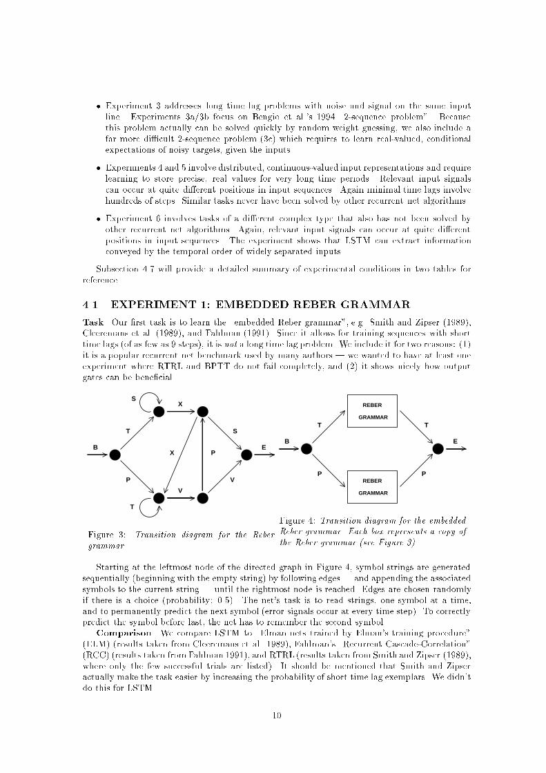
� Experiment 3 addresses long time lag problems with noise and signal on the same inputline. Experiments 3a/3b focus on Bengio et al.'s 1994 \2-sequence problem". Becausethis problem actually can be solved quickly by random weight guessing, we also include afar more di�cult 2-sequence problem (3c) which requires to learn real-valued, conditionalexpectations of noisy targets, given the inputs.� Experiments 4 and 5 involve distributed, continuous-valued input representations and requirelearning to store precise, real values for very long time periods. Relevant input signalscan occur at quite di�erent positions in input sequences. Again minimal time lags involvehundreds of steps. Similar tasks never have been solved by other recurrent net algorithms.� Experiment 6 involves tasks of a di�erent complex type that also has not been solved byother recurrent net algorithms. Again, relevant input signals can occur at quite di�erentpositions in input sequences. The experiment shows that LSTM can extract informationconveyed by the temporal order of widely separated inputs.Subsection 4.7 will provide a detailed summary of experimental conditions in two tables forreference.4.1 EXPERIMENT 1: EMBEDDED REBER GRAMMARTask. Our �rst task is to learn the \embedded Reber grammar", e.g. Smith and Zipser (1989),Cleeremans et al. (1989), and Fahlman (1991). Since it allows for training sequences with shorttime lags (of as few as 9 steps), it is not a long time lag problem. We include it for two reasons: (1)it is a popular recurrent net benchmark used by many authors | we wanted to have at least oneexperiment where RTRL and BPTT do not fail completely, and (2) it shows nicely how outputgates can be bene�cial.B

T

SX

X P

V

T

P V

S

EFigure 3: Transition diagram for the Rebergrammar. B

T

P

E

T

P

GRAMMAR

GRAMMAR

REBER

REBERFigure 4: Transition diagram for the embeddedReber grammar. Each box represents a copy ofthe Reber grammar (see Figure 3).Starting at the leftmost node of the directed graph in Figure 4, symbol strings are generatedsequentially (beginning with the empty string) by following edges | and appending the associatedsymbols to the current string | until the rightmost node is reached. Edges are chosen randomlyif there is a choice (probability: 0.5). The net's task is to read strings, one symbol at a time,and to permanently predict the next symbol (error signals occur at every time step). To correctlypredict the symbol before last, the net has to remember the second symbol.Comparison. We compare LSTM to \Elman nets trained by Elman's training procedure"(ELM) (results taken from Cleeremans et al. 1989), Fahlman's \Recurrent Cascade-Correlation"(RCC) (results taken fromFahlman 1991), and RTRL (results taken from Smith and Zipser (1989),where only the few successful trials are listed). It should be mentioned that Smith and Zipseractually make the task easier by increasing the probability of short time lag exemplars. We didn'tdo this for LSTM. 10

method hidden units # weights learning rate % of success success afterRTRL 3 � 170 0.05 \some fraction" 173,000RTRL 12 � 494 0.1 \some fraction" 25,000ELM 15 � 435 0 >200,000RCC 7-9 � 119-198 50 182,000LSTM 4 blocks, size 1 264 0.1 100 39,740LSTM 3 blocks, size 2 276 0.1 100 21,730LSTM 3 blocks, size 2 276 0.2 97 14,060LSTM 4 blocks, size 1 264 0.5 97 9,500LSTM 3 blocks, size 2 276 0.5 100 8,440Table 1: EXPERIMENT 1: Embedded Reber grammar: percentage of successful trials and numberof sequence presentations until success for RTRL (results taken from Smith and Zipser 1989),\Elman net trained by Elman's procedure" (results taken from Cleeremans et al. 1989), \RecurrentCascade-Correlation" (results taken from Fahlman 1991) and our new approach (LSTM). Weightnumbers in the �rst 4 rows are estimates | the corresponding papers don't provide all the technicaldetails. Only LSTM almost always learns to solve the task (only two failures out of 150 trials).Even when we ignore the unsuccessful trials of the other approaches, LSTM learns much faster(the number of required training examples in the bottom row varies between 3,800 and 24,100).Training/Testing. We use a local input/output representation (7 input units, 7 outputunits). Following Fahlman, we use 256 training strings and 256 separate test strings. The trainingset is generated randomly; training exemplars are picked randomly from the training set. Testsequences are generated randomly, too, but sequences already used in the training set are notused for testing. After string presentation, all activations are reinitialized with zeros. A trial isconsidered successful if all string symbols of all sequences in both test set and training set arepredicted correctly | that is, if the output unit(s) corresponding to the possible next symbol(s)is(are) always the most active ones.Architectures. Architectures for RTRL, ELM, RCC are reported in the references listedabove. For LSTM, we use 3 (4) memory cell blocks. Each block has 2 (1) memory cells. Theoutput layer's only incoming connections originate at memory cells. Each memory cell and eachgate unit receives incoming connections from all memory cells and gate units (the hidden layer isfully connected | less connectivity may work as well). The input layer has forward connectionsto all units in the hidden layer. The gate units are biased. These architecture parameters make iteasy to store at least 3 input signals (architectures 3-2 and 4-1 are employed to obtain comparablenumbers of weights for both architectures: 264 for 4-1 and 276 for 3-2). Other parameters may beappropriate as well, however. All sigmoid functions are logistic with output range [0; 1], except forh, whose range is [�1; 1], and g, whose range is [�2; 2]. All weights are initialized in [�0:2; 0:2],except for the output gate biases, which are initialized to -1, -2, and -3, respectively (see abuseproblem, solution (2) of Section 3). We tried learning rates of 0.1, 0.2 and 0.5.Results. We use 3 di�erent, randomly generated pairs of training and test sets. With eachsuch pair we run 10 trials with di�erent initial weights. See Table 1 for results (mean of 30trials). Unlike the other methods, LSTM always learns to solve the task. Even when we ignorethe unsuccessful trials of the other approaches, LSTM learns much faster.Importance of output gates. The experiment provides a nice example where the output gateis truly bene�cial. Learning to store the �rst T or P should not perturb activations representingthe more easily learnable transitions of the original Reber grammar. This is the job of the outputgates. Without output gates, we did not achieve fast learning.11

Method Delay p Learning rate # weights % Successful trials Success afterRTRL 4 1.0 36 78 1,043,000RTRL 4 4.0 36 56 892,000RTRL 4 10.0 36 22 254,000RTRL 10 1.0-10.0 144 0 > 5,000,000RTRL 100 1.0-10.0 10404 0 > 5,000,000BPTT 100 1.0-10.0 10404 0 > 5,000,000CH 100 1.0 10506 33 32,400LSTM 100 1.0 10504 100 5,040Table 2: Task 2a: Percentage of successful trials and number of training sequences until success,for \Real-Time Recurrent Learning" (RTRL), \Back-Propagation Through Time" (BPTT), neuralsequence chunking (CH), and the new method (LSTM). Table entries refer to means of 18 trials.With 100 time step delays, only CH and LSTM achieve successful trials. Even when we ignore theunsuccessful trials of the other approaches, LSTM learns much faster.4.2 EXPERIMENT 2: NOISE-FREE AND NOISY SEQUENCESTask 2a: noise-free sequences with long time lags. There are p+ 1 possible input symbolsdenoted a1; :::; ap�1; ap = x; ap+1 = y. ai is \locally" represented by the p+ 1-dimensional vectorwhose i-th component is 1 (all other components are 0). A net with p + 1 input units and p + 1output units sequentially observes input symbol sequences, one at a time, permanently tryingto predict the next symbol | error signals occur at every single time step. To emphasize the\long time lag problem", we use a training set consisting of only two very similar sequences:(y; a1; a2; : : : ; ap�1; y) and (x; a1; a2; : : : ; ap�1; x). Each is selected with probability 0.5. To predictthe �nal element, the net has to learn to store a representation of the �rst element for p timesteps.We compare \Real-Time Recurrent Learning" for fully recurrent nets (RTRL), \Back-Propa-gation Through Time" (BPTT), the sometimes very successful 2-net \Neural Sequence Chunker"(CH, Schmidhuber 1992b), and our new method (LSTM). In all cases, weights are initialized in[-0.2,0.2]. Due to limited computation time, training is stopped after 5 million sequence presen-tations. A successful run is one that ful�lls the following criterion: after training, during 10,000successive, randomly chosen input sequences, the maximal absolute error of all output units isalways below 0:25.Architectures. RTRL: one self-recurrent hidden unit, p+1 non-recurrent output units. Eachlayer has connections from all layers below. All units use the logistic activation function sigmoidin [0,1].BPTT: same architecture as the one trained by RTRL.CH: both net architectures like RTRL's, but one has an additional output for predicting thehidden unit of the other one (see Schmidhuber 1992b for details).LSTM: like with RTRL, but the hidden unit is replaced by a memory cell and an input gate(no output gate required). g is the logistic sigmoid, and h is the identity function h : h(x) = x; 8x.Memory cell and input gate are added once the error has stopped decreasing (see abuse problem:solution (1) in Section 3).Results. Using RTRL and a short 4 time step delay (p = 4), 79 of all trials were successful.No trial was successful with p = 10. With long time lags, only the neural sequence chunkerand LSTM achieved successful trials, while BPTT and RTRL failed. With p = 100, the 2-netsequence chunker solved the task in only 13 of all trials. LSTM, however, always learned to solvethe task. Comparing successful trials only, LSTM learned much faster. See Table 2 for details. Itshould be mentioned, however, that a hierarchical chunker can also always quickly solve this task(Schmidhuber 1992c, 1993). 12

Task 2b: no local regularities. With the task above, the chunker sometimes learns tocorrectly predict the �nal element, but only because of predictable local regularities in the inputstream that allow for compressing the sequence. In an additional, more di�cult task (involvingmany more di�erent possible sequences), we remove compressibility by replacing the determin-istic subsequence (a1; a2; : : : ; ap�1) by a random subsequence (of length p � 1) over the alpha-bet a1; a2; : : : ; ap�1. We obtain 2 classes (two sets of sequences) f(y; ai1 ; ai2; : : : ; aip�1 ; y) j 1 �i1; i2; : : : ; ip�1 � p � 1g and f(x; ai1; ai2 ; : : : ; aip�1 ; x) j 1 � i1; i2; : : : ; ip�1 � p � 1g. Again, everynext sequence element has to be predicted. The only totally predictable targets, however, are xand y, which occur at sequence ends. Training exemplars are chosen randomly from the 2 classes.Architectures and parameters are the same as in Experiment 2a. A successful run is one thatful�lls the following criterion: after training, during 10,000 successive, randomly chosen inputsequences, the maximal absolute error of all output units is below 0:25 at sequence end.Results. As expected, the chunker failed to solve this task (so did BPTT and RTRL, ofcourse). LSTM, however, was always successful. On average (mean of 18 trials), success forp = 100 was achieved after 5,680 sequence presentations. This demonstrates that LSTM does notrequire sequence regularities to work well.Task 2c: very long time lags | no local regularities. This is the most di�cult task inthis subsection. To our knowledge no other recurrent net algorithm can solve it. Now there are p+4possible input symbols denoted a1; :::; ap�1; ap; ap+1 = e; ap+2 = b; ap+3 = x; ap+4 = y. a1; :::; apare also called \distractor symbols". Again, ai is locally represented by the p+4-dimensional vectorwhose ith component is 1 (all other components are 0). A net with p+4 input units and 2 outputunits sequentially observes input symbol sequences, one at a time. Training sequences are randomlychosen from the union of two very similar subsets of sequences: f(b; y; ai1; ai2 ; : : : ; aiq+k; e; y) j 1�i1; i2; : : : ; iq+k � qg and f(b; x; ai1; ai2 ; : : : ; aiq+k ; e; x) j 1 � i1; i2; : : : ; iq+k � qg. To produce atraining sequence, we (1) randomly generate a sequence pre�x of length q + 2, (2) randomlygenerate a sequence su�x of additional elements (6= b; e; x; y) with probability 910 or, alternatively,an e with probability 110 . In the latter case, we (3) conclude the sequence with x or y, dependingon the second element. For a given k, this leads to a uniform distribution on the possible sequenceswith length q + k + 4. The minimal sequence length is q + 4; the expected length is4 + 1Xk=0 110( 910)k(q + k) = q + 14:The expected number of occurrences of element ai; 1 � i � p, in a sequence is q+10p � qp . Thegoal is to predict the last symbol, which always occurs after the \trigger symbol" e. Error signalsare generated only at sequence ends. To predict the �nal element, the net has to learn to store arepresentation of the second element for at least q+ 1 time steps (until it sees the trigger symbole). Success is de�ned as \prediction error (for �nal sequence element) of both output units alwaysbelow 0:2, for 10,000 successive, randomly chosen input sequences".13

q (time lag �1) p (# random inputs) qp # weights Success after50 50 1 364 30,000100 100 1 664 31,000200 200 1 1264 33,000500 500 1 3064 38,0001,000 1,000 1 6064 49,0001,000 500 2 3064 49,0001,000 200 5 1264 75,0001,000 100 10 664 135,0001,000 50 20 364 203,000Table 3: Task 2c: LSTM with very long minimal time lags q + 1 and a lot of noise. p is thenumber of available distractor symbols (p + 4 is the number of input units). qp is the expectednumber of occurrences of a given distractor symbol in a sequence. The rightmost column lists thenumber of training sequences required by LSTM (BPTT, RTRL and the other competitors haveno chance of solving this task). If we let the number of distractor symbols (and weights) increasein proportion to the time lag, learning time increases very slowly. The lower block illustrates theexpected slow-down due to increased frequency of distractor symbols.Architecture/Learning. The net has p + 4 input units and 2 output units. Weights areinitialized in [-0.2,0.2]. To avoid too much learning time variance due to di�erent weight initial-izations, the hidden layer gets two memory cells (two cell blocks of size 1 | although one wouldbe su�cient). There are no other hidden units. The output layer receives connections only frommemory cells. Memory cells and gate units receive connections from input units, memory cellsand gate units (i.e., the hidden layer is fully connected). No bias weights are used. h and g arelogistic sigmoids with output ranges [�1; 1] and [�2; 2], respectively. The learning rate is 0.01.Note that the minimal time lag is q+ 1 | the net never sees short training sequences facilitatingthe classi�cation of long test sequences.Results. 20 trials were made for all tested pairs (p; q). Table 3 lists the mean of the numberof training sequences required by LSTM to achieve success (BPTT and RTRL have no chance ofsolving non-trivial tasks with minimal time lags of 1000 steps).Scaling. Table 3 shows that if we let the number of input symbols (and weights) increasein proportion to the time lag, learning time increases very slowly. This is a another remarkableproperty of LSTM not shared by any other method we are aware of. Indeed, RTRL and BPTTare far from scaling reasonably | instead, they appear to scale exponentially, and appear quiteuseless when the time lags exceed as few as 10 steps.Distractor in uence. In Table 3, the column headed by qp gives the expected frequency ofdistractor symbols. Increasing this frequency decreases learning speed, an e�ect due to weightoscillations caused by frequently observed input symbols.4.3 EXPERIMENT 3: NOISE AND SIGNAL ON SAME CHANNELThis experiment serves to illustrate that LSTM does not encounter fundamental problems if noiseand signal are mixed on the same input line. We initially focus on Bengio et al.'s simple 1994\2-sequence problem"; in Experiment 3c we will then pose a more challenging 2-sequence problem.Task 3a (\2-sequence problem"). The task is to observe and then classify input sequences.There are two classes, each occurring with probability 0.5. There is only one input line. Onlythe �rst N real-valued sequence elements convey relevant information about the class. Sequenceelements at positions t > N are generated by a Gaussian with mean zero and variance 0.2. CaseN = 1: the �rst sequence element is 1.0 for class 1, and -1.0 for class 2. Case N = 3: the �rstthree elements are 1.0 for class 1 and -1.0 for class 2. The target at the sequence end is 1.0 for14

T N stop: ST1 stop: ST2 # weights ST2: fraction misclassi�ed100 3 27,380 39,850 102 0.000195100 1 58,370 64,330 102 0.0001171000 3 446,850 452,460 102 0.000078Table 4: Task 3a: Bengio et al.'s 2-sequence problem. T is minimal sequence length. N is thenumber of information-conveying elements at sequence begin. The column headed by ST1 (ST2)gives the number of sequence presentations required to achieve stopping criterion ST1 (ST2). Therightmost column lists the fraction of misclassi�ed post-training sequences (with absolute error >0.2) from a test set consisting of 2560 sequences (tested after ST2 was achieved). All values aremeans of 10 trials. We discovered, however, that this problem is so simple that random weightguessing solves it faster than LSTM and any other method we know of.class 1 and 0.0 for class 2. Correct classi�cation is de�ned as \absolute output error at sequenceend below 0.2". Given a constant T, the sequence length is randomly selected between T and T +T/10 (a di�erence to Bengio et al.'s problem is that they also permit shorter sequences of lengthT/2).For the 2-sequence problem, the best method among the six tested by Bengio et al. (1994)was multigrid random search (sequence lengths 50{100; no precise stopping criterion mentioned),which solved the problem after 6,400 sequence presentations, with �nal classi�cation error 0.06.In more recent work, Bengio and Frasconi were able to improve their results: an EM-approachwas reported to solve the problem within 2,900 trials.Guessing. We discovered that the 2-sequence problem is so simple that it can quickly besolved by random weight guessing. We ran an experiment with one input unit, 10 hidden units,one output unit, and logistic activation functions sigmoid in [0:0; 1:0]. Each hidden unit sees theinput unit, the output unit, and itself; the output unit sees all other units; all units have biasweights. By randomly guessing weights in [-100.0,100.0], it is possible to solve the problem in only718 trials on average. Using Bengio et al.'s 3-parameter architecture for the \latch problem" (asimple version of the 2-sequence problem that allows for input tuning instead of weight tuning), theproblem was solved in only 22 trials on average, due to the tiny parameter space. See Schmidhuberand Hochreiter (1996) or Hochreiter and Schmidhuber (1997) for additional results in this vein.LSTM architecture. We use a 3-layer net with 1 input unit, 1 output unit, and 3 cell blocksof size 1. The output layer receives connections only from memory cells. Memory cells and gateunits receive inputs from input units, memory cells and gate units, and have bias weights. Gateunits and output unit are logistic sigmoid in [0; 1], h in [�1; 1], and g in [�2; 2].Training/Testing. All weights (except the bias weights to gate units) are randomly initializedin the range [�0:1; 0:1]. The �rst input gate bias is initialized with �1:0, the second with �3:0,and the third with �5:0. The �rst output gate bias is initialized with �2:0, the second with �4:0and the third with �6:0. The precise initialization values hardly matter though, as con�rmed byadditional experiments. The learning rate is 1.0. All activations are reset to zero at the beginningof a new sequence.We stop training (and judge the task as being solved) according to the following criteria: ST1:none of 256 sequences from a randomly chosen test set is misclassi�ed. ST2: ST1 is satis�ed, andmean absolute test set error is below 0.01. In case of ST2, an additional test set consisting of 2560randomly chosen sequences is used to determine the fraction of misclassi�ed sequences.Results. See Table 4. The results are means of 10 trials with di�erent weight initializationsin the range [�0:1; 0:1]. LSTM is able to solve this problem, though by far not as fast as randomweight guessing (see paragraph \Guessing" above). Clearly, this trivial problem does not provide avery good testbed to compare performance of various non-trivial algorithms. Still, it demonstratesthat LSTM does not encounter fundamental problems when faced with signal and noise on thesame channel. 15

T N stop: ST1 stop: ST2 # weights ST2: fraction misclassi�ed100 3 41,740 43,250 102 0.00828100 1 74,950 78,430 102 0.015001000 1 481,060 485,080 102 0.01207Table 5: Task 3b: modi�ed 2-sequence problem. Same as in Table 4, but now the information-conveying elements are also perturbed by noise.T N stop # weights fraction misclassi�ed av. di�erence to mean100 3 269,650 102 0.00558 0.014100 1 565,640 102 0.00441 0.012Table 6: Task 3c: modi�ed, more challenging 2-sequence problem. Same as in Table 4, but withnoisy real-valued targets. The system has to learn the conditional expectations of the targets giventhe inputs. The rightmost column provides the average di�erence between network output andexpected target. Unlike 3a and 3b, this task cannot be solved quickly by random weight guessing.Task 3b. Architecture, parameters, etc. like in Task 3a, but now with Gaussian noise (mean0 and variance 0.2) added to the information-conveying elements (t <= N ). We stop training(and judge the task as being solved) according to the following, slightly rede�ned criteria: ST1:less than 6 out of 256 sequences from a randomly chosen test set are misclassi�ed. ST2: ST1 issatis�ed, and mean absolute test set error is below 0.04. In case of ST2, an additional test setconsisting of 2560 randomly chosen sequences is used to determine the fraction of misclassi�edsequences.Results. See Table 5. The results represent means of 10 trials with di�erent weight initializa-tions. LSTM easily solves the problem.Task 3c. Architecture, parameters, etc. like in Task 3a, but with a few essential changes thatmake the task non-trivial: the targets are 0.2 and 0.8 for class 1 and class 2, respectively, andthere is Gaussian noise on the targets (mean 0 and variance 0.1; st.dev. 0.32). To minimize meansquared error, the system has to learn the conditional expectations of the targets given the inputs.Misclassi�cation is de�ned as \absolute di�erence between output and noise-free target (0.2 forclass 1 and 0.8 for class 2) > 0.1. " The network output is considered acceptable if the meanabsolute di�erence between noise-free target and output is below 0.015. Since this requires highweight precision, Task 3c (unlike 3a and 3b) cannot be solved quickly by random guessing.Training/Testing. The learning rate is 0:1. We stop training according to the followingcriterion: none of 256 sequences from a randomly chosen test set is misclassi�ed, and meanabsolute di�erence between noise free target and output is below 0.015. An additional test setconsisting of 2560 randomly chosen sequences is used to determine the fraction of misclassi�edsequences.Results. See Table 6. The results represent means of 10 trials with di�erent weight initial-izations. Despite the noisy targets, LSTM still can solve the problem by learning the expectedtarget values.4.4 EXPERIMENT 4: ADDING PROBLEMThe di�cult task in this section is of a type that has never been solved by other recurrent net al-gorithms. It shows that LSTM can solve long time lag problems involving distributed, continuous-valued representations.Task. Each element of each input sequence is a pair of components. The �rst componentis a real value randomly chosen from the interval [�1; 1]; the second is either 1.0, 0.0, or -1.0,16

T minimal lag # weights # wrong predictions Success after100 50 93 1 out of 2560 74,000500 250 93 0 out of 2560 209,0001000 500 93 1 out of 2560 853,000Table 7: EXPERIMENT 4: Results for the Adding Problem. T is the minimal sequence length,T=2 the minimal time lag. \# wrong predictions" is the number of incorrectly processed sequences(error > 0.04) from a test set containing 2560 sequences. The rightmost column gives the numberof training sequences required to achieve the stopping criterion. All values are means of 10 trials.For T = 1000 the number of required training examples varies between 370,000 and 2,020,000,exceeding 700,000 in only 3 cases.and is used as a marker: at the end of each sequence, the task is to output the sum of the �rstcomponents of those pairs that are marked by second components equal to 1.0. Sequences haverandom lengths between the minimal sequence length T and T + T10 . In a given sequence exactlytwo pairs are marked as follows: we �rst randomly select and mark one of the �rst ten pairs(whose �rst component we call X1). Then we randomly select and mark one of the �rst T2 � 1still unmarked pairs (whose �rst component we call X2). The second components of all remainingpairs are zero except for the �rst and �nal pair, whose second components are -1. (In the rare casewhere the �rst pair of the sequence gets marked, we set X1 to zero.) An error signal is generatedonly at the sequence end: the target is 0:5+ X1+X24:0 (the sum X1+X2 scaled to the interval [0; 1]).A sequence is processed correctly if the absolute error at the sequence end is below 0.04.Architecture. We use a 3-layer net with 2 input units, 1 output unit, and 2 cell blocks of size2. The output layer receives connections only from memory cells. Memory cells and gate unitsreceive inputs from memory cells and gate units (i.e., the hidden layer is fully connected | lessconnectivity may work as well). The input layer has forward connections to all units in the hiddenlayer. All non-input units have bias weights. These architecture parameters make it easy to storeat least 2 input signals (a cell block size of 1 works well, too). All activation functions are logisticwith output range [0; 1], except for h, whose range is [�1; 1], and g, whose range is [�2; 2].State drift versus initial bias. Note that the task requires storing the precise values ofreal numbers for long durations | the system must learn to protect memory cell contents againsteven minor internal state drift (see Section 3). To study the signi�cance of the drift problem,we make the task even more di�cult by biasing all non-input units, thus arti�cially inducinginternal state drift. All weights (including the bias weights) are randomly initialized in the range[�0:1; 0:1]. Following Section 3's remedy for state drifts, the �rst input gate bias is initialized with�3:0, the second with �6:0 (though the precise values hardly matter, as con�rmed by additionalexperiments).Training/Testing. The learning rate is 0.5. Training is stopped if the average training erroris below 0.01, and the 2000 most recent sequences were processed correctly.Results. With a test set consisting of 2560 randomly chosen sequences, the average test seterror was always below 0.01, and there were never more than 3 incorrectly processed sequences.Table 7 shows details.The experiment demonstrates: (1) LSTM is able to work well with distributed representations.(2) LSTM is able to learn to perform calculations involving continuous values. (3) Since the systemmanages to store continuous values without deterioration for minimal delays of T2 time steps, thereis no signi�cant, harmful internal state drift.4.5 EXPERIMENT 5: MULTIPLICATION PROBLEMOne may argue that LSTM is a bit biased towards tasks such as the Adding Problem from theprevious subsection. Solutions to the Adding Problem may exploit the CEC's built-in integration17

T minimal lag # weights nseq # wrong predictions MSE Success after100 50 93 140 139 out of 2560 0.0223 482,000100 50 93 13 14 out of 2560 0.0139 1,273,000Table 8: EXPERIMENT 5: Results for the Multiplication Problem. T is minimal sequence length,T=2 is minimal time lag. We test on a test set containing 2560 sequences as soon as less thannseq of the 2000 most recent training sequences lead to error > 0.04. \# wrong predictions" is thenumber of test sequences with error > 0.04. MSE is the mean squared error on the test set. Therightmost column lists numbers of training sequences required to achieve the stopping criterion.All values are means of 10 trials.capabilities. Although this CEC property may be viewed as a feature rather than a disadvantage(integration seems to be a natural subtask of many tasks occurring in the real world), the questionarises whether LSTM can also solve tasks with inherently non-integrative solutions. To test this,we change the problem by requiring the �nal target to equal the product (instead of the sum) ofearlier marked inputs.Task. Like the task in section 4.4, except that the �rst component of each pair is a real valuerandomly chosen from the interval [0; 1]. In the rare case where the �rst pair of the input sequencegets marked, we set X1 to 1.0. The target at sequence end is the product X1 �X2.Architecture. Like in section 4.4. All weights (including the bias weights) are randomlyinitialized in the range [�0:1; 0:1].Training/Testing. The learning rate is 0.1. We test performance twice: as soon as lessthan nseq of the 2000 most recent training sequences lead to absolute errors exceeding 0.04, wherenseq = 140, and nseq = 13. Why these values? nseq = 140 is su�cient to learn storage of therelevant inputs. It is not enough though to �ne-tune the precise �nal outputs. nseq = 13, however,leads to quite satisfactory results.Results. For nseq = 140 (nseq = 13) with a test set consisting of 2560 randomly chosensequences, the average test set error was always below 0.026 (0.013), and there were never morethan 170 (15) incorrectly processed sequences. Table 8 shows details. (A net with additionalstandard hidden units or with a hidden layer above the memory cells may learn the �ne-tuningpart more quickly.)The experiment demonstrates: LSTM can solve tasks involving both continuous-valued repre-sentations and non-integrative information processing.4.6 EXPERIMENT 6: TEMPORAL ORDERIn this subsection, LSTM solves di�cult tasks of another type that have never been solved byother recurrent net algorithms. The experiment shows that LSTM is able to extract informationconveyed by the temporal order of widely separated inputs.Task 6a: two relevant, widely separated symbols. The goal is to classify sequences.Elements and targets are represented locally (input vectors with only one non-zero bit). Thesequence starts with anE, ends with a B (the \trigger symbol") and otherwise consists of randomlychosen symbols from the set fa; b; c; dg except for two elements at positions t1 and t2 that are eitherX or Y . The sequence length is randomly chosen between 100 and 110, t1 is randomly chosenbetween 10 and 20, and t2 is randomly chosen between 50 and 60. There are 4 sequence classesQ;R; S; U which depend on the temporal order of X and Y . The rules are: X;X ! Q; X;Y !R; Y;X ! S; Y; Y ! U .Task 6b: three relevant, widely separated symbols. Again, the goal is to classifysequences. Elements/targets are represented locally. The sequence starts with an E, ends witha B (the \trigger symbol"), and otherwise consists of randomly chosen symbols from the setfa; b; c; dg except for three elements at positions t1; t2 and t3 that are either X or Y . The sequence18

length is randomly chosen between 100 and 110, t1 is randomly chosen between 10 and 20, t2 israndomly chosen between 33 and 43, and t3 is randomly chosen between 66 and 76. There are 8sequence classes Q;R; S; U; V;A;B;C which depend on the temporal order of the Xs and Y s. Therules are: X;X;X ! Q; X;X; Y ! R; X;Y;X ! S; X;Y; Y ! U ; Y;X;X ! V ; Y;X; Y !A; Y; Y;X ! B; Y; Y; Y ! C.There are as many output units as there are classes. Each class is locally represented by abinary target vector with one non-zero component. With both tasks, error signals occur only atthe end of a sequence. The sequence is classi�ed correctly if the �nal absolute error of all outputunits is below 0.3.Architecture. We use a 3-layer net with 8 input units, 2 (3) cell blocks of size 2 and 4(8) output units for Task 6a (6b). Again all non-input units have bias weights, and the outputlayer receives connections from memory cells only. Memory cells and gate units receive inputsfrom input units, memory cells and gate units (i.e., the hidden layer is fully connected | lessconnectivity may work as well). The architecture parameters for Task 6a (6b) make it easy tostore at least 2 (3) input signals. All activation functions are logistic with output range [0; 1],except for h, whose range is [�1; 1], and g, whose range is [�2; 2].Training/Testing. The learning rate is 0.5 (0.1) for Experiment 6a (6b). Training is stoppedonce the average training error falls below 0.1 and the 2000 most recent sequences were classi�edcorrectly. All weights are initialized in the range [�0:1; 0:1]. The �rst input gate bias is initializedwith �2:0, the second with �4:0, and (for Experiment 6b) the third with �6:0 (again, we con�rmedby additional experiments that the precise values hardly matter).Results. With a test set consisting of 2560 randomly chosen sequences, the average test seterror was always below 0.1, and there were never more than 3 incorrectly classi�ed sequences.Table 9 shows details.The experiment shows that LSTM is able to extract information conveyed by the temporalorder of widely separated inputs. In Task 6a, for instance, the delays between �rst and secondrelevant input and between second relevant input and sequence end are at least 30 time steps.task # weights # wrong predictions Success afterTask 6a 156 1 out of 2560 31,390Task 6b 308 2 out of 2560 571,100Table 9: EXPERIMENT 6: Results for the Temporal Order Problem. \# wrong predictions" isthe number of incorrectly classi�ed sequences (error > 0.3 for at least one output unit) from atest set containing 2560 sequences. The rightmost column gives the number of training sequencesrequired to achieve the stopping criterion. The results for Task 6a are means of 20 trials; thosefor Task 6b of 10 trials.Typical solutions. In Experiment 6a, how does LSTM distinguish between temporal orders(X;Y ) and (Y;X)? One of many possible solutions is to store the �rst X or Y in cell block 1, andthe second X=Y in cell block 2. Before the �rst X=Y occurs, block 1 can see that it is still emptyby means of its recurrent connections. After the �rst X=Y , block 1 can close its input gate. Onceblock 1 is �lled and closed, this fact will become visible to block 2 (recall that all gate units andall memory cells receive connections from all non-output units).Typical solutions, however, require only one memory cell block. The block stores the �rst Xor Y ; once the second X=Y occurs, it changes its state depending on the �rst stored symbol.Solution type 1 exploits the connection between memory cell output and input gate unit | thefollowing events cause di�erent input gate activations: \X occurs in conjunction with a �lledblock"; \X occurs in conjunction with an empty block". Solution type 2 is based on a strongpositive connection between memory cell output and memory cell input. The previous occurrenceof X (Y ) is represented by a positive (negative) internal state. Once the input gate opens for thesecond time, so does the output gate, and the memory cell output is fed back to its own input.19

This causes (X;Y ) to be represented by a positive internal state, because X contributes to thenew internal state twice (via current internal state and cell output feedback). Similarly, (Y;X)gets represented by a negative internal state.4.7 SUMMARY OF EXPERIMENTAL CONDITIONSThe two tables in this subsection provide an overview of the most important LSTM parametersand architectural details for Experiments 1{6. The conditions of the simple experiments 2a and2b di�er slightly from those of the other, more systematic experiments, due to historical reasons.1 2 3 4 5 6 7 8 9 10 11 12 13 14 15Task p lag b s in out w c ogb igb bias h g �1-1 9 9 4 1 7 7 264 F -1,-2,-3,-4 r ga h1 g2 0.11-2 9 9 3 2 7 7 276 F -1,-2,-3 r ga h1 g2 0.11-3 9 9 3 2 7 7 276 F -1,-2,-3 r ga h1 g2 0.21-4 9 9 4 1 7 7 264 F -1,-2,-3,-4 r ga h1 g2 0.51-5 9 9 3 2 7 7 276 F -1,-2,-3 r ga h1 g2 0.52a 100 100 1 1 101 101 10504 B no og none none id g1 1.02b 100 100 1 1 101 101 10504 B no og none none id g1 1.02c-1 50 50 2 1 54 2 364 F none none none h1 g2 0.012c-2 100 100 2 1 104 2 664 F none none none h1 g2 0.012c-3 200 200 2 1 204 2 1264 F none none none h1 g2 0.012c-4 500 500 2 1 504 2 3064 F none none none h1 g2 0.012c-5 1000 1000 2 1 1004 2 6064 F none none none h1 g2 0.012c-6 1000 1000 2 1 504 2 3064 F none none none h1 g2 0.012c-7 1000 1000 2 1 204 2 1264 F none none none h1 g2 0.012c-8 1000 1000 2 1 104 2 664 F none none none h1 g2 0.012c-9 1000 1000 2 1 54 2 364 F none none none h1 g2 0.013a 100 100 3 1 1 1 102 F -2,-4,-6 -1,-3,-5 b1 h1 g2 1.03b 100 100 3 1 1 1 102 F -2,-4,-6 -1,-3,-5 b1 h1 g2 1.03c 100 100 3 1 1 1 102 F -2,-4,-6 -1,-3,-5 b1 h1 g2 0.14-1 100 50 2 2 2 1 93 F r -3,-6 all h1 g2 0.54-2 500 250 2 2 2 1 93 F r -3,-6 all h1 g2 0.54-3 1000 500 2 2 2 1 93 F r -3,-6 all h1 g2 0.55 100 50 2 2 2 1 93 F r r all h1 g2 0.16a 100 40 2 2 8 4 156 F r -2,-4 all h1 g2 0.56b 100 24 3 2 8 8 308 F r -2,-4,-6 all h1 g2 0.1Table 10: Summary of experimental conditions for LSTM, Part I. 1st column: task number. 2ndcolumn: minimal sequence length p. 3rd column: minimal number of steps between most recentrelevant input information and teacher signal. 4th column: number of cell blocks b. 5th column:block size s. 6th column: number of input units in. 7th column: number of output units out. 8thcolumn: number of weights w. 9th column: c describes connectivity: \F" means \output layerreceives connections from memory cells; memory cells and gate units receive connections frominput units, memory cells and gate units"; \B" means \each layer receives connections from alllayers below". 10th column: initial output gate bias ogb, where \r" stands for \randomly chosenfrom the interval [�0:1; 0:1]" and \no og" means \no output gate used". 11th column: initial inputgate bias igb (see 10th column). 12th column: which units have bias weights? \b1" stands for \allhidden units", \ga" for \only gate units", and \all" for \all non-input units". 13th column: thefunction h, where \id" is identity function, \h1" is logistic sigmoid in [�2; 2]. 14th column: thelogistic function g, where \g1" is sigmoid in [0; 1], \g2" in [�1; 1]. 15th column: learning rate �.20

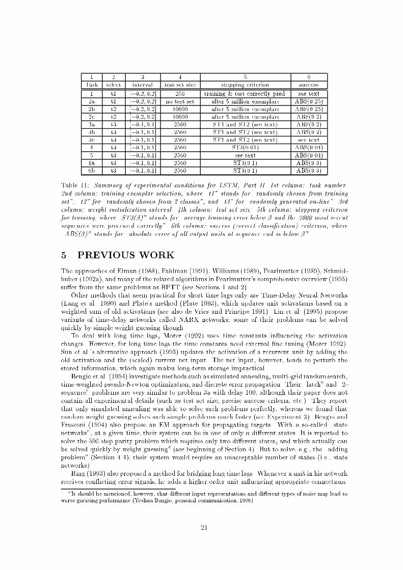
1 2 3 4 5 6Task select interval test set size stopping criterion success1 t1 [�0:2; 0:2] 256 training & test correctly pred. see text2a t1 [�0:2; 0:2] no test set after 5 million exemplars ABS(0.25)2b t2 [�0:2; 0:2] 10000 after 5 million exemplars ABS(0.25)2c t2 [�0:2; 0:2] 10000 after 5 million exemplars ABS(0.2)3a t3 [�0:1; 0:1] 2560 ST1 and ST2 (see text) ABS(0.2)3b t3 [�0:1; 0:1] 2560 ST1 and ST2 (see text) ABS(0.2)3c t3 [�0:1; 0:1] 2560 ST1 and ST2 (see text) see text4 t3 [�0:1; 0:1] 2560 ST3(0.01) ABS(0.04)5 t3 [�0:1; 0:1] 2560 see text ABS(0.04)6a t3 [�0:1; 0:1] 2560 ST3(0.1) ABS(0.3)6b t3 [�0:1; 0:1] 2560 ST3(0.1) ABS(0.3)Table 11: Summary of experimental conditions for LSTM, Part II. 1st column: task number.2nd column: training exemplar selection, where \t1" stands for \randomly chosen from trainingset", \t2" for \randomly chosen from 2 classes", and \t3" for \randomly generated on-line". 3rdcolumn: weight initialization interval. 4th column: test set size. 5th column: stopping criterionfor training, where \ST3(�)" stands for \average training error below � and the 2000 most recentsequences were processed correctly". 6th column: success (correct classi�cation) criterion, where\ABS(�)" stands for \absolute error of all output units at sequence end is below �".5 PREVIOUS WORKThe approaches of Elman (1988), Fahlman (1991), Williams (1989), Pearlmutter (1989), Schmid-huber (1992a), and many of the related algorithms in Pearlmutter's comprehensive overview (1995)su�er from the same problems as BPTT (see Sections 1 and 2).Other methods that seem practical for short time lags only are Time-Delay Neural Networks(Lang et al. 1990) and Plate's method (Plate 1993), which updates unit activations based on aweighted sum of old activations (see also de Vries and Principe 1991). Lin et al. (1995) proposevariants of time-delay networks called NARX networks; some of their problems can be solvedquickly by simple weight guessing though.To deal with long time lags, Mozer (1992) uses time constants in uencing the activationchanges. However, for long time lags the time constants need external �ne tuning (Mozer 1992).Sun et al.'s alternative approach (1993) updates the activation of a recurrent unit by adding theold activation and the (scaled) current net input. The net input, however, tends to perturb thestored information, which again makes long-term storage impractical.Bengio et al. (1994) investigate methods such as simulated annealing, multi-grid random search,time-weighted pseudo-Newton optimization, and discrete error propagation. Their \latch" and \2-sequence" problems are very similar to problem 3a with delay 100, although their paper does notcontain all experimental details (such as test set size, precise success criteria, etc.). They reportthat only simulated annealing was able to solve such problems perfectly, whereas we found thatrandom weight guessing solves such simple problems much faster (see Experiment 3). Bengio andFrasconi (1994) also propose an EM approach for propagating targets. With n so-called \statenetworks", at a given time, their system can be in one of only n di�erent states. It is reported tosolve the 500 step parity problem which requires only two di�erent states, and which actually canbe solved quickly by weight guessing4 (see beginning of Section 4). But to solve, e.g., the \addingproblem" (Section 4.4), their system would require an unacceptable number of states (i.e., statenetworks).Ring (1993) also proposed a method for bridging long time lags. Whenever a unit in his networkreceives con icting error signals, he adds a higher order unit in uencing appropriate connections.4It should be mentioned, however, that di�erent input representations and di�erent types of noise may lead toworse guessing performance (Yoshua Bengio, personal communication, 1996).21

Although his approach can sometimes be extremely fast, to bridge a time lag involving 100 stepsmay require the addition of 100 units. Also, Ring's net does not generalize to unseen lag durations.Puskorius and Feldkamp (1994) used Kalman �lter techniques to improve recurrent net per-formance. There is no reason to believe, however, that their Kalman Filter Trained RecurrentNetworks (1994) will be useful for very long minimal time lags. In fact, they use \a derivativediscount factor imposed to decay exponentially the e�ects of past dynamic derivatives."Schmidhuber's hierarchical chunker system does have a capability to bridge arbitrary timelags, but only if there is local predictability across the subsequence causing the time lag (seeSchmidhuber 1992b, 1993; and Mozer 1992). For instance, in his postdoctoral thesis (1993),Schmidhuber uses hierarchical recurrent nets to rapidly solve certain grammar learning tasksinvolving minimal time lags in excess of 1000 steps. The performance of chunker systems, however,deteriorates as the noise level increases. Chunker systems can be augmented by LSTM though tocombine the advantages of both.LSTM is not the �rst method that involves multiplicative units. For instance, Watrous andKuhn (1992) also use multiplicative inputs in second order nets. Some di�erences to LSTM are:(1) Watrous and Kuhn's architecture has no linear units to enforce constant error ow. It isnot designed to solve long time lag problems. (2) It has fully connected second-order sigma-piunits, while the LSTM architecture's only multiplicative units are the gate units. (3) Watrousand Kuhn's algorithm costs O(W 2) operations per time step, ours only O(W ). See also Millerand Giles (1993) for additional work on multiplicative inputs. As we recently discovered, however,simple weight guessing solves some of Miller and Giles' problems more quickly than the algorithmsthey investigate (Schmidhuber and Hochreiter, 1996).6 DISCUSSIONLimitations of LSTM.� The particularly e�cient truncated backprop version of the LSTM algorithm won't easilysolve problems similar to \strongly delayed XOR problems", where the goal is to compute theXOR of two widely separated inputs that previously occurred somewhere in a noisy sequence.The reason is that storing only one of the inputs won't help to reduce the expected error |the task is non-decomposable in the sense that it is impossible to incrementally reduce theerror by �rst solving an easier subgoal. In theory, this limitation can be circumvented byusing the full gradient (perhaps with additional conventional hidden units receiving inputfrom the memory cells). This will increase computational complexity though.� Each memory cell block needs two additional units (input and output gate). In comparisonto standard recurrent nets, however, this does not increase the number of weights by morethan a factor of 9: each conventional hidden unit is replaced by at most 3 units in theLSTM architecture, increasing the number of weights by a factor of 32 in the fully connectedcase. Note, however, that our experiments use quite comparable weight numbers for thearchitectures of LSTM and competing approaches.� Generally speaking, due to its constant error ow through CECs within memory cells, LSTMruns into problems similar to those of feedforward nets seeing the entire input string at once.For instance, there are tasks that can be quickly solved by randomweight guessing but not bythe truncated LSTM algorithm with small weight initializations, such as the 500-step parityproblem (see introduction to Section 4). Here, LSTM's problems are similar to the ones ofa feedforward net with 500 inputs, trying to solve 500-bit parity. Indeed LSTM typicallybehaves much like a feedforward net trained by backprop that sees the entire input. Butthat's also precisely why it so clearly outperforms previous approaches on many non-trivialtasks with signi�cant search spaces. 22

� LSTM does not have any problems with the notion of \recency" that go beyond those ofother approaches. All gradient-based approaches, however, su�er from practical inability toprecisely count discrete time steps. If it makes a di�erence whether a certain signal occurred99 or 100 steps ago, then an additional counting mechanism seems necessary. Easier tasks,however, such as one that only requires to make a di�erence between, say, 3 and 11 steps,do not pose any problems to LSTM. For instance, by generating an appropriate negativeconnection between memory cell output and input, LSTM can give more weight to recentinputs and learn decays where necessary.Advantages of LSTM.� The constant error backpropagation within memory cells results in LSTM's ability to bridgevery long time lags.� LSTM works well for long time lag problems involving noise, distributed representations, andcontinuous values. LSTM does not require an a priori choice of a �nite number of states.� LSTM generalizes well even in cases where the positions of widely separated, relevant inputsin the input sequence do not matter. Unlike previous approaches, ours quickly learns todistinguish between two or more widely separated occurrences of a particular element in aninput sequence, without depending on appropriate short time lag training exemplars.� There appears to be no need for parameter �ne tuning. LSTM works well over a broad rangeof parameters such as learning rate, input gate bias and output gate bias. For instance, tosome readers the learning rates used in our experiments may seem large. However, a largelearning rate pushes the output gates towards zero, thus automatically countermanding itsown negative e�ects.� The LSTM algorithm's update complexity for fully recurrent nets is essentially that of BPTT(namely just O(W ), where W is the number of weights). This is excellent in comparison toother approaches such as RTRL. Unlike full BPTT, however, LSTM is local in space.� Since memory cells can be plugged into any feedforward or recurrent net, and since anygradient-based algorithm can be plugged into any other (all we need is the chain rule),LSTM can be seamlessly integrated into feedforward or recurrent nets trained by RTRL,BPTT, backprop, and other gradient-based approaches.7 CONCLUSIONIn hindsight, LSTM's architecture seems simple and obvious to the authors. Each memory cell'sinternal architecture guarantees constant error ow within its constant error carrousel CEC. Thisprovides the basis for bridging very long time lags. Two gate units learn to open and close accessto error ow within each memory cell's CEC. The multiplicative input gate a�ords protection ofthe CEC from perturbation by irrelevant inputs. Likewise, the multiplicative output gate protectsother units from perturbation by currently irrelevant memory contents.Future work. To �nd out about the practical limitations of LSTM, we intend to apply it toreal world data. Application areas will include (1) time series prediction, (2) music composition,and (3) speech processing. 23

8 ACKNOWLEDGMENTSThanks to Mike Mozer, Wilfried Brauer, Nic Schraudolph, and several anonymous referees for valu-able comments and suggestions that helped to improve a previous version of this paper (Hochreiterand Schmidhuber 1995). This work was supported by DFG grant SCHM 942/3-1 from \DeutscheForschungsgemeinschaft".APPENDIXA.1 ALGORITHM DETAILSIn what follows, the index k ranges over output units, i ranges over hidden units, cj stands forthe j-th memory cell block, cvj denotes the v-th unit of memory cell block cj , u; l;m stand forarbitrary units, t ranges over all time steps of a given input sequence.The gate unit logistic sigmoid (with range [0; 1]) used in the experiments isf(x) = 11 + exp(�x) . (3)The function h (with range [�1; 1]) used in the experiments ish(x) = 21 + exp(�x) � 1 . (4)The function g (with range [�2; 2]) used in the experiments isg(x) = 41 + exp(�x) � 2 . (5)Forward pass.The net input and the activation of hidden unit i areneti(t) = Xu wiuyu(t � 1) (6)yi(t) = fi(neti(t)) .The net input and the activation of inj arenetinj (t) = Xu winjuyu(t� 1) (7)yinj (t) = finj (netinj (t)) .The net input and the activation of outj arenetoutj (t) = Xu woutjuyu(t� 1) (8)youtj (t) = foutj (netoutj (t)) .The net input netcvj , the internal state scvj , and the output activation ycvj of the v-th memorycell of memory cell block cj are:netcvj (t) = Xu wcvjuyu(t� 1) (9)scvj (t) = scvj (t � 1) + yinj (t)g �netcvj (t)�ycvj (t) = youtj (t)h(scvj (t)) .24

The net input and the activation of output unit k arenetk(t) = Xu: u not a gate wkuyu(t� 1)yk(t) = fk(netk(t)) .The backward pass to be described later is based on the following truncated backprop formulae.Approximate derivatives for truncated backprop. The truncated version (see Section 3)only approximates the partial derivatives, which is re ected by the \�tr" signs in the notationbelow. It truncates error ow once it leaves memory cells or gate units. Truncation ensures thatthere are no loops across which an error that left some memory cell through its input or inputgate can reenter the cell through its output or output gate. This in turn ensures constant error ow through the memory cell's CEC.In the truncated backprop version, the following derivatives are replaced by zero:@netinj (t)@yu(t � 1) �tr 0 8u;@netoutj (t)@yu(t � 1) �tr 0 8u;and @netcj (t)@yu(t � 1) �tr 0 8u:Therefore we get @yinj (t)@yu(t� 1) = f 0inj (netinj (t)) @netinj (t)@yu(t� 1) �tr 0 8u;@youtj (t)@yu(t � 1) = f 0outj (netoutj (t))@netoutj (t)@yu(t� 1) �tr 0 8u;and@ycj (t)@yu(t � 1) = @ycj (t)@netoutj (t) @netoutj (t)@yu(t � 1) + @ycj (t)@netinj (t) @netinj (t)@yu(t� 1) + @ycj (t)@netcj (t) @netcj (t)@yu(t � 1) �tr 0 8u:This implies for all wlm not on connections to cvj ; inj ; outj (that is, l 62 fcvj ; inj; outjg):@ycvj (t)@wlm =Xu @ycvj (t)@yu(t � 1) @yu(t� 1)@wlm �tr 0:The truncated derivatives of output unit k are:@yk(t)@wlm = f 0k(netk(t)) Xu: u not a gate wku@yu(t � 1)@wlm + �klym(t� 1)! �tr (10)f 0k(netk(t))0@Xj SjXv=1 �cvj lwkcvj @ycvj (t� 1)@wlm +Xj ��injl + �outjl� SjXv=1wkcvj @ycvj (t � 1)@wlm +Xi: i hidden unit wki@yi(t� 1)@wlm + �klym(t� 1)! =f 0k(netk(t))8>>>>><>>>>>: ym(t � 1) l = kwkcvj @ycvj (t�1)@wlm l = cvjPSjv=1wkcvj @ycvj (t�1)@wlm l = inj OR l = outjPi: i hidden unit wki @yi(t�1)@wlm l otherwise ,25

where � is the Kronecker delta (�ab = 1 if a = b and 0 otherwise), and Sj is the size of memorycell block cj . The truncated derivatives of a hidden unit i that is not part of a memory cell are:@yi(t)@wlm = f 0i (neti(t))@neti(t)@wlm �tr �lif 0i (neti(t))ym(t� 1) . (11)(Note: here it would be possible to use the full gradient without a�ecting constant error owthrough internal states of memory cells.)Cell block cj 's truncated derivatives are:@yinj (t)@wlm = f 0inj (netinj (t))@netinj (t)@wlm �tr �inj lf 0inj (netinj (t))ym(t � 1) . (12)@youtj (t)@wlm = f 0outj (netoutj (t))@netoutj (t)@wlm �tr �outj lf 0outj (netoutj (t))ym(t � 1) . (13)@scvj (t)@wlm = @scvj (t� 1)@wlm + @yinj (t)@wlm g �netcvj (t)�+ yinj (t)g0 �netcvj (t)� @netcvj (t)@wlm �tr (14)��inj l + �cvj l� @scvj (t� 1)@wlm + �injl @yinj (t)@wlm g �netcvj (t)�+�cvj lyinj (t)g0 �netcvj (t)� @netcvj (t)@wlm =��inj l + �cvj l� @scvj (t� 1)@wlm + �injlf 0inj (netinj (t)) g �netcvj (t)� ym(t � 1) +�cvj l yinj (t) g0 �netcvj (t)� ym(t� 1) .@ycvj (t)@wlm = @youtj (t)@wlm h(scvj (t)) + h0(scvj (t))@scvj (t)@wlm youtj (t) �tr (15)�outjl @youtj (t)@wlm h(scvj (t)) + ��injl + �cvj l�h0(scvj (t))@scvj (t)@wlm youtj (t) .To e�ciently update the system at time t, the only (truncated) derivatives that need to be storedat time t � 1 are @scvj (t�1)@wlm , where l = cvj or l = inj .Backward pass. We will describe the backward pass only for the particularly e�cient \truncatedgradient version" of the LSTM algorithm. For simplicity we will use equal signs even whereapproximations are made according to the truncated backprop equations above.The squared error at time t is given byE(t) = Xk: k output unit �tk(t) � yk(t)�2 , (16)where tk(t) is output unit k's target at time t.Time t's contribution to wlm's gradient-based update with learning rate � is�wlm(t) = �� @E(t)@wlm . (17)We de�ne some unit l's error at time step t byel(t) := � @E(t)@netl(t) . (18)Using (almost) standard backprop, we �rst compute updates for weights to output units (l = k),weights to hidden units (l = i) and weights to output gates (l = outj). We obtain (compareformulae (10), (11), (13)):l = k (output) : ek(t) = f 0k(netk(t)) �tk(t) � yk(t)� , (19)26

l = i (hidden) : ei(t) = f 0i (neti(t)) Xk: k output unit wkiek(t) , (20)l = outj (output gates) : (21)eoutj (t) = f 0outj (netoutj (t))0@ SjXv=1h(scvj (t)) Xk: k output unit wkcvj ek(t)1A .For all possible l time t's contribution to wlm's update is�wlm(t) = � el(t) ym(t� 1) . (22)The remaining updates for weights to input gates (l = inj) and to cell units (l = cvj ) are lessconventional. We de�ne some internal state scvj 's error:escvj := � @E(t)@scvj (t) = (23)foutj (netoutj (t)) h0(scvj (t)) Xk: k output unit wkcvj ek(t) .We obtain for l = inj or l = cvj ; v = 1; : : : ; Sj�@E(t)@wlm = SjXv=1 escvj (t)@scvj (t)@wlm . (24)The derivatives of the internal states with respect to weights and the corresponding weightupdates are as follows (compare expression (14)): l = inj (input gates) : (25)@scvj (t)@winjm = @scvj (t � 1)@winjm + g(netcvj (t)) f 0inj (netinj (t)) ym(t � 1) ;therefore time t's contribution to winjm's update is (compare expression (10)):�winjm(t) = � SjXv=1 escvj (t) @scvj (t)@winjm . (26)Similarly we get (compare expression (14)): l = cvj (memory cells) : (27)@scvj (t)@wcvjm = @scvj (t� 1)@wcvjm + g0(netcvj (t)) finj (netinj (t)) ym(t � 1) ;therefore time t's contribution to wcvjm's update is (compare expression (10)):�wcvjm(t) = �escvj (t)@scvj (t)@wcvjm . (28)All we need to implement for the backward pass are equations (19), (20), (21), (22), (23), (25),(26), (27), (28). Each weight's total update is the sum of the contributions of all time steps.Computational complexity. LSTM's update complexity per time step isO(KH +KCS +HI +CSI) = O(W ); (29)27

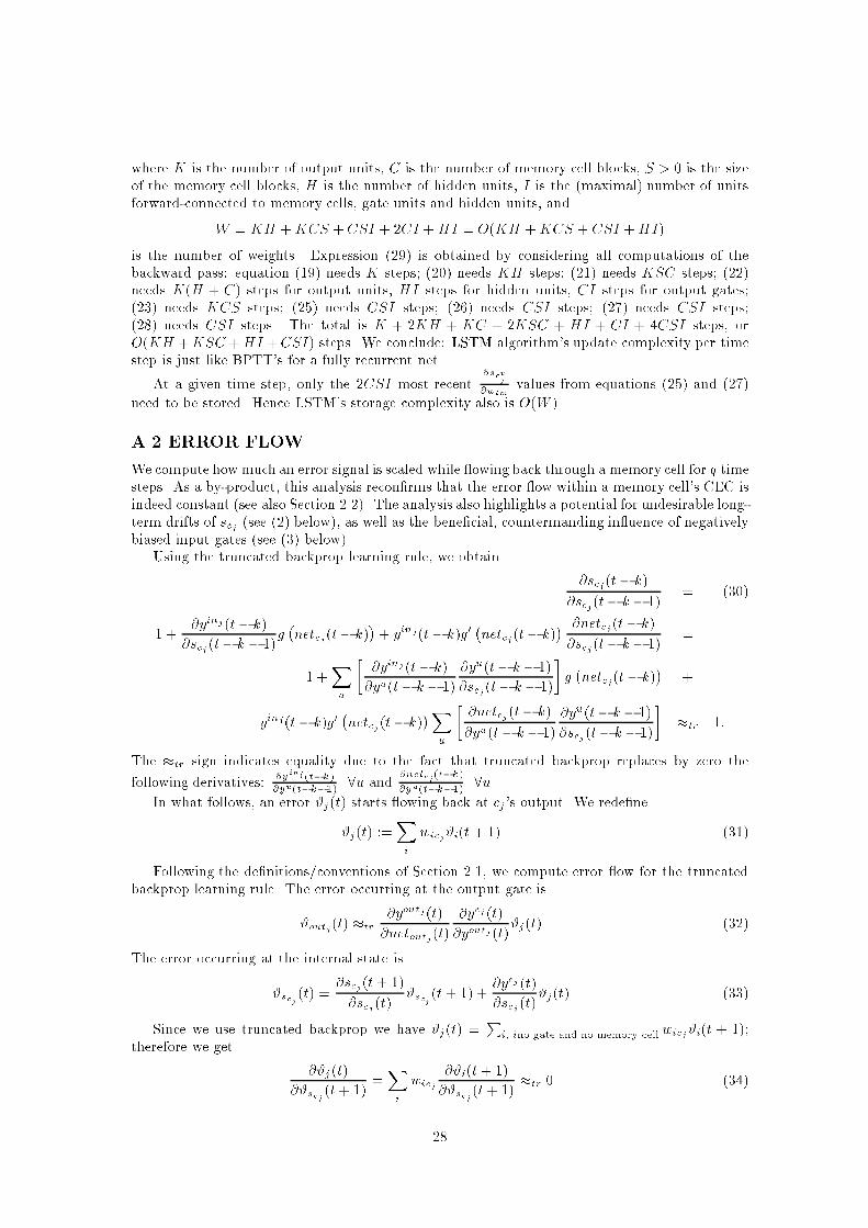
where K is the number of output units, C is the number of memory cell blocks, S > 0 is the sizeof the memory cell blocks, H is the number of hidden units, I is the (maximal) number of unitsforward-connected to memory cells, gate units and hidden units, andW = KH +KCS +CSI + 2CI +HI = O(KH +KCS + CSI +HI)is the number of weights. Expression (29) is obtained by considering all computations of thebackward pass: equation (19) needs K steps; (20) needs KH steps; (21) needs KSC steps; (22)needs K(H + C) steps for output units, HI steps for hidden units, CI steps for output gates;(23) needs KCS steps; (25) needs CSI steps; (26) needs CSI steps; (27) needs CSI steps;(28) needs CSI steps. The total is K + 2KH + KC + 2KSC + HI + CI + 4CSI steps, orO(KH +KSC +HI +CSI) steps. We conclude: LSTM algorithm's update complexity per timestep is just like BPTT's for a fully recurrent net.At a given time step, only the 2CSI most recent @scvj@wlm values from equations (25) and (27)need to be stored. Hence LSTM's storage complexity also is O(W ).A.2 ERROR FLOWWe compute how much an error signal is scaled while owing back through a memory cell for q timesteps. As a by-product, this analysis recon�rms that the error ow within a memory cell's CEC isindeed constant (see also Section 2.2). The analysis also highlights a potential for undesirable long-term drifts of scj (see (2) below), as well as the bene�cial, countermanding in uence of negativelybiased input gates (see (3) below).Using the truncated backprop learning rule, we obtain @scj (t � k)@scj (t� k � 1) = (30)1 + @yinj (t � k)@scj (t� k � 1)g �netcj (t� k)�+ yinj (t � k)g0 �netcj (t� k)� @netcj (t � k)@scj (t� k � 1) =1 +Xu � @yinj (t � k)@yu(t � k � 1) @yu(t� k � 1)@scj (t� k � 1)� g �netcj (t � k)� +yinj (t � k)g0 �netcj (t� k)�Xu � @netcj (t� k)@yu(t � k � 1) @yu(t� k � 1)@scj (t� k � 1)� �tr 1:The �tr sign indicates equality due to the fact that truncated backprop replaces by zero thefollowing derivatives: @yinj (t�k)@yu(t�k�1) 8u and @netcj (t�k)@yu(t�k�1) 8u.In what follows, an error #j(t) starts owing back at cj's output. We rede�ne#j(t) :=Xi wicj#i(t + 1) . (31)Following the de�nitions/conventions of Section 2.1, we compute error ow for the truncatedbackprop learning rule. The error occurring at the output gate is#outj (t) �tr @youtj (t)@netoutj (t) @ycj (t)@youtj (t)#j(t) . (32)The error occurring at the internal state is#scj (t) = @scj (t+ 1)@scj (t) #scj (t+ 1) + @ycj (t)@scj (t)#j(t) . (33)Since we use truncated backprop we have #j(t) = Pi, ino gate and no memory cellwicj#i(t + 1);therefore we get @#j(t)@#scj (t+ 1) =Xi wicj @#i(t+ 1)@#scj (t + 1) �tr 0 . (34)28

The previous equations (33) and (34) imply constant error ow through internal states ofmemory cells: @#scj (t)@#scj (t+ 1) = @scj (t + 1)@scj (t) �tr 1 . (35)The error occurring at the memory cell input is#cj (t) = @g(netcj (t))@netcj (t) @scj (t)@g(netcj (t))#scj (t) . (36)The error occurring at the input gate is#inj(t) �tr @yinj (t)@netinj (t) @scj (t)@yinj (t))#scj (t) . (37)No external error ow. Errors are propagated back from units l to unit v along outgoingconnections with weights wlv. This \external error" (note that for conventional units there isnothing but external error) at time t is#ev(t) = @yv(t)@netv(t)Xl @netl(t + 1)@yv(t) #l(t + 1) . (38)We obtain @#ev(t� 1)@#j(t) = (39)@yv(t � 1)@netv(t� 1) �@#outj (t)@#j(t) @netoutj (t)@yv(t� 1) + @#inj (t)@#j(t) @netinj (t)@yv(t� 1) + @#cj (t)@#j(t) @netcj (t)@yv(t� 1)� �tr 0 .We observe: the error #j arriving at the memory cell output is not backpropagated to units v viaexternal connections to inj ; outj; cj.Error ow within memory cells. We now focus on the error back ow within a memorycell's CEC. This is actually the only type of error ow that can bridge several time steps. Supposeerror #j(t) arrives at cj 's output at time t and is propagated back for q steps until it reaches injor the memory cell input g(netcj ). It is scaled by a factor of @#v(t�q)@#j(t) , where v = inj; cj. We �rstcompute @#scj (t� q)@#j(t) �tr 8<: @ycj (t)@scj (t) q = 0@scj (t�q+1)@scj (t�q) @#scj (t�q+1)@#j(t) q > 0 . (40)Expanding equation (40), we obtain@#v(t� q)@#j(t) �tr @#v(t � q)@#scj (t� q) @#scj (t � q)@#j(t) �tr (41)@#v(t � q)@#scj (t� q) 1Ym=q @scj (t�m+ 1)@scj (t�m) ! @ycj (t)@scj (t) �tryoutj (t)h0(scj (t))� g0(netcj (t� q)yinj (t� q) v = cjg(netcj (t � q)f 0inj (netinj (t� q)) v = inj .Consider the factors in the previous equation's last expression. Obviously, error ow is scaledonly at times t (when it enters the cell) and t � q (when it leaves the cell), but not in between(constant error ow through the CEC). We observe:29

(1) The output gate's e�ect is: youtj (t) scales down those errors that can be reduced earlyduring training without using the memory cell. Likewise, it scales down those errors resultingfrom using (activating/deactivating) the memory cell at later training stages | without the outputgate, the memory cell might for instance suddenly start causing avoidable errors in situations thatalready seemed under control (because it was easy to reduce the corresponding errors withoutmemory cells). See \output weight con ict" and \abuse problem" in Sections 2/3.(2) If there are large positive or negative scj (t) values (because scj has drifted since time stept� q), then h0(scj (t)) may be small (assuming that h is a logistic sigmoid). See Section 3. Driftsof the memory cell's internal state scj can be countermanded by negatively biasing the input gateinj (see Section 3 and next point). Recall from Section 3 that the precise bias value does notmatter much.(3) yinj (t � q) and f 0inj (netinj (t � q)) are small if the input gate is negatively biased (assumefinj is a logistic sigmoid). However, the potential signi�cance of this is negligible compared to thepotential signi�cance of drifts of the internal state scj .Some of the factors above may scale down LSTM's overall error ow, but not in a mannerthat depends on the length of the time lag. The ow will still be much more e�ective than anexponentially (of order q) decaying ow without memory cells.ReferencesBengio, Y. and Frasconi, P. (1994). Credit assignment through time: Alternatives to backpropaga-tion. In Cowan, J. D., Tesauro, G., and Alspector, J., editors, Advances in Neural InformationProcessing Systems 6, pages 75{82. San Mateo, CA: Morgan Kaufmann.Bengio, Y., Simard, P., and Frasconi, P. (1994). Learning long-term dependencies with gradientdescent is di�cult. IEEE Transactions on Neural Networks, 5(2):157{166.Cleeremans, A., Servan-Schreiber, D., and McClelland, J. L. (1989). Finite-state automata andsimple recurrent networks. Neural Computation, 1:372{381.de Vries, B. and Principe, J. C. (1991). A theory for neural networks with time delays. InLippmann, R. P., Moody, J. E., and Touretzky, D. S., editors, Advances in Neural InformationProcessing Systems 3, pages 162{168. San Mateo, CA: Morgan Kaufmann.Doya, K. and Yoshizawa, S. (1989). Adaptive neural oscillator using continuous-time back-propagation learning. Neural Networks, 2:375{385.Elman, J. L. (1988). Finding structure in time. Technical Report CRL 8801, Center for Researchin Language, University of California, San Diego.Fahlman, S. E. (1991). The recurrent cascade-correlation learning algorithm. In Lippmann, R. P.,Moody, J. E., and Touretzky, D. S., editors, Advances in Neural Information ProcessingSystems 3, pages 190{196. San Mateo, CA: Morgan Kaufmann.Hochreiter, J. (1991). Untersuchungen zu dynamischen neuronalen Netzen. Diploma the-sis, Institut f�ur Informatik, Lehrstuhl Prof. Brauer, Technische Universit�at M�unchen. Seewww7.informatik.tu-muenchen.de/~hochreit.Hochreiter, S. and Schmidhuber, J. (1995). Long short-term memory. Technical Report FKI-207-95, Fakult�at f�ur Informatik, Technische Universit�at M�unchen.Hochreiter, S. and Schmidhuber, J. (1996). Bridging long time lags by weight guessing and \LongShort-Term Memory". In Silva, F. L., Principe, J. C., and Almeida, L. B., editors, Spa-tiotemporal models in biological and arti�cial systems, pages 65{72. IOS Press, Amsterdam,Netherlands. Serie: Frontiers in Arti�cial Intelligence and Applications, Volume 37.30

Hochreiter, S. and Schmidhuber, J. (1997). LSTM can solve hard long time lag problems. InAdvances in Neural Information Processing Systems 9. MIT Press, Cambridge MA. Presentedat NIPS 96.Lang, K., Waibel, A., and Hinton, G. E. (1990). A time-delay neural network architecture forisolated word recognition. Neural Networks, 3:23{43.Lin, T., Horne, B. G., Tino, P., and Giles, C. L. (1995). Learning long-term dependencies isnot as di�cult with NARX recurrent neural networks. Technical Report UMIACS-TR-95-78and CS-TR-3500, Institute for Advanced Computer Studies, University of Maryland, CollegePark, MD 20742.Miller, C. B. and Giles, C. L. (1993). Experimental comparison of the e�ect of order in recurrentneural networks. International Journal of Pattern Recognition and Arti�cial Intelligence,7(4):849{872.Mozer, M. C. (1989). A focused back-propagation algorithm for temporal sequence recognition.Complex Systems, 3:349{381.Mozer, M. C. (1992). Induction of multiscale temporal structure. In Moody, J. E., Hanson, S. J.,and Lippman, R. P., editors, Advances in Neural Information Processing Systems 4, pages275{282. San Mateo, CA: Morgan Kaufmann.Pearlmutter, B. A. (1989). Learning state space trajectories in recurrent neural networks. NeuralComputation, 1(2):263{269.Pearlmutter, B. A. (1995). Gradient calculations for dynamic recurrent neural networks: A survey.IEEE Transactions on Neural Networks, 6(5):1212{1228.Plate, T. A. (1993). Holographic recurrent networks. In S. J. Hanson, J. D. C. and Giles, C. L.,editors, Advances in Neural Information Processing Systems 5, pages 34{41. San Mateo, CA:Morgan Kaufmann.Pollack, J. B. (1991). Language induction by phase transition in dynamical recognizers. InLippmann, R. P., Moody, J. E., and Touretzky, D. S., editors, Advances in Neural InformationProcessing Systems 3, pages 619{626. San Mateo, CA: Morgan Kaufmann.Puskorius, G. V. and Feldkamp, L. A. (1994). Neurocontrol of nonlinear dynamical systems withKalman �lter trained recurrent networks. IEEE Transactions on Neural Networks, 5(2):279{297.Ring, M. B. (1993). Learning sequential tasks by incrementally adding higher orders. In S. J. Han-son, J. D. C. and Giles, C. L., editors, Advances in Neural Information Processing Systems5, pages 115{122. Morgan Kaufmann.Robinson, A. J. and Fallside, F. (1987). The utility driven dynamic error propagation network.Technical Report CUED/F-INFENG/TR.1, Cambridge University Engineering Department.Schmidhuber, J. (1989). A local learning algorithm for dynamic feedforward and recurrent net-works. Connection Science, 1(4):403{412.Schmidhuber, J. (1992a). A �xed size storage O(n3) time complexity learning algorithm for fullyrecurrent continually running networks. Neural Computation, 4(2):243{248.Schmidhuber, J. (1992b). Learning complex, extended sequences using the principle of historycompression. Neural Computation, 4(2):234{242.Schmidhuber, J. (1992c). Learning unambiguous reduced sequence descriptions. In Moody, J. E.,Hanson, S. J., and Lippman, R. P., editors, Advances in Neural Information Processing Sys-tems 4, pages 291{298. San Mateo, CA: Morgan Kaufmann.31

Schmidhuber, J. (1993). Netzwerkarchitekturen, Zielfunktionen und Kettenregel. Habilitationss-chrift, Institut f�ur Informatik, Technische Universit�at M�unchen.Schmidhuber, J. and Hochreiter, S. (1996). Guessing can outperform many long time lag algo-rithms. Technical Report IDSIA-19-96, IDSIA.Silva, G. X., Amaral, J. D., Langlois, T., and Almeida, L. B. (1996). Faster training of recurrentnetworks. In Silva, F. L., Principe, J. C., and Almeida, L. B., editors, Spatiotemporal models inbiological and arti�cial systems, pages 168{175. IOS Press, Amsterdam, Netherlands. Series:Frontiers in Arti�cial Intelligence and Applications, Volume 37.Smith, A. W. and Zipser, D. (1989). Learning sequential structures with the real-time recurrentlearning algorithm. International Journal of Neural Systems, 1(2):125{131.Sun, G., Chen, H., and Lee, Y. (1993). Time warping invariant neural networks. In S. J. Hanson,J. D. C. and Giles, C. L., editors, Advances in Neural Information Processing Systems 5,pages 180{187. San Mateo, CA: Morgan Kaufmann.Watrous, R. L. and Kuhn, G. M. (1992). Induction of �nite-state languages using second-orderrecurrent networks. Neural Computation, 4:406{414.Williams, R. J. (1989). Complexity of exact gradient computation algorithms for recurrent neuralnetworks. Technical Report NU-CCS-89-27, Boston: Northeastern University, College ofComputer Science.Williams, R. J. and Peng, J. (1990). An e�cient gradient-based algorithm for on-line training ofrecurrent network trajectories. Neural Computation, 4:491{501.Williams, R. J. and Zipser, D. (1992). Gradient-based learning algorithms for recurrent networksand their computational complexity. In Chauvin, Y. and Rumelhart, D. E., editors, Back-propagation: Theory, Architectures and Applications. Hillsdale, NJ: Erlbaum.

32