Long-duration Bonds and Sovereign Defaults∗

Juan Carlos Hatchondo Leonardo Martinez

January 15, 2009

Abstract

This paper extends the baseline framework used in recent quantitative studies of sovereigndefault by assuming that the government can borrow using long-duration bonds. This con-trasts with previous studies, which assume that the government can borrow using bondsthat mature after one quarter. We solve the model assuming that the government issuesbonds with a duration similar to the average duration of sovereign bonds in emergingeconomies and show that the model is able to generate a substantially higher and morevolatile interest rate. This narrows the gap between the predictions of the model and thedata, which indicates that the introduction of long-duration bonds may be a useful tool forfuture research about emerging economies. Our analysis is also relevant for the study ofother credit markets.

JEL classification: F34, F41.Keywords: Sovereign Default, Endogenous Borrowing Constraints, Bond Duration,

Debt Dilution, Markov Perfect Equilibrium.

∗For comments and suggestions, we thank our colleagues at the Federal Reserve Bank of Richmond, andseminar and conference participants at Universidad de Malaga, Universitat Autonoma de Barcelona, Universityof Bern, Universidad Nacional de Tucuman, the Central Bank of Uruguay, the 2008 Wegmans Conference, the2008 Meeting of the Canadian Macroeconomics Study Group, the 2008 Workshop of the Latin American FinancialNetwork, the 2008 Warwick Workshop on Sovereign and Public Debt and Default, and the IMF Institute. E-mails: JuanCarlos.Hatchondo@rich.frb.org; Leonardo.Martinez@rich.frb.org. The views expressed here do notnecessarily reflect those of the Federal Reserve Bank of Richmond or the Federal Reserve System.

1

1 Introduction

Business cycles in small emerging economies differ from those in developed economies. Emerg-

ing economies feature interest rates that are higher, more volatile and countercyclical (interest

rates are usually acyclical in developed economies), and have higher output volatility, higher

volatility of consumption relative to income, and more countercyclical net exports (see Aguiar

and Gopinath (2007), Neumeyer and Perri (2005), and Uribe and Yue (2006)). Due to the high

volatility and countercyclicality of the interest rate in emerging economies, a state-dependent

interest rate schedule is a key ingredient in any model designed to explain the cyclical behavior

of aggregate quantities and prices in these economies. In this respect, some studies assume an

exogenous interest rate schedule.1 Others present models with microfoundations for the interest

rate schedule based on the risk of default. This is the approach taken by recent quantitative stud-

ies of sovereign default, which extend the framework proposed by Eaton and Gersovitz (1981).2

The setup studied in our paper belongs to the second class of models.

As in previous studies of sovereign default, we analyze a small open economy that receives a

stochastic endowment stream of a single tradable good. The objective of the government is to

maximize the expected utility of private agents. The government makes two decisions in every

period. First, it decides whether to default on previously issued debt. The cost of defaulting is

represented by an endowment loss that is incurred in the default period. Second, the government

decides how much to borrow or save. The government can borrow (save) by issuing (buying) non-

contingent bonds that are priced in a competitive market inhabited by a large number of identical

risk-neutral lenders. Lenders have perfect information regarding the economy’s endowment.

The main difference between our paper and previous studies is that while previous quantita-

tive studies assume that sovereign bonds mature after one quarter, we assume that the govern-

1See, for instance, Aguiar and Gopinath (2007), Neumeyer and Perri (2005), Schmitt-Grohe and Uribe (2003),and Uribe and Yue (2006).

2See, for instance, Aguiar and Gopinath (2006), Arellano (2008), Arellano and Ramanarayanan (2008), Baiand Zhang (2006), Benjamin and Wright (2008), Cuadra and Sapriza (2006, 2008), D’Erasmo (2008), Eyigungor(2006), Hatchondo et al. (2006, 2007, 2008), Lizarazo (2005, 2006), Mendoza and Yue (2008), and Yue (2005).These models share blueprints with the models used in quantitative studies of household bankruptcy—see, forexample, Athreya (2002), Athreya et al. (2007a,b), Chatterjee et al. (2007a), Chatterjee et al. (2007b), Li andSarte (2006), Livshits et al. (2008), and Sanchez (2008).

2

ment issues bonds that pay an infinite stream of coupons until a default is declared. The coupon

payments promised decrease at a constant rate. This assumption allows us to introduce debt

instruments with long duration in a simple and tractable way: the number of state variables is

independent of the duration of debt.

We solve the model assuming that the government issues bonds that have a duration of

four years—similar to the average duration in emerging economies, as documented by Cruces

et al. (2002) and Cunningham et al. (2001)—and show that the predictions of the model change

significantly compared to the predictions obtained with one-quarter bonds. The mean and the

standard deviation of the spread—extra yield over the risk-free rate—in simulations of the model

increase. The model with long-duration bonds is also able to replicate other salient features

of emerging economies, like the excessive volatility of consumption compared to GDP and the

countercyclicality of the trade balance. Thus, our results narrow the gap between the predictions

of the baseline model of sovereign default and the data, which indicates that introducing long-

duration bonds may be a useful tool for future research about emerging economies.

The rest of the article proceeds as follows. Section 2 introduces the model. Section 3 presents

a recursive formulation. Section 4 discusses the parameter values used to solve the model. Section

5 presents the results. Section 6 discusses the robustness of our results. Section 7 concludes.

2 The model

The basic framework studied in this paper follows previous work that extends the model of

sovereign default presented by Eaton and Gersovitz (1981), and studies its quantitative perfor-

mance. The main difference between the model we present and the baseline framework is that

our model allows us to study long-duration bonds.

3

2.1 The environment

There is a single tradable good. The economy receives a stochastic endowment stream of this

good, where

log(yt) = (1 − ρ) µ + ρ log(yt−1) + εt,

with |ρ| < 1, and εt ∼ N (0, σ2ǫ ).

The objective of the government is to maximize the present expected discounted value of

future utility flows of the representative agent in the economy, namely

E

[

∞∑

t=0

βtu (ct)

]

,

where β denotes the subjective discount factor and the utility function is assumed to display a

constant coefficient of relative risk aversion, denoted by σ. That is,

u (c) =c(1−σ) − 1

1 − σ.

The government makes two decisions in each period. First, it decides whether to default. A

default implies that the government repudiates all current and future debt obligations contracted

in the past. The cost of a default is represented by the loss of an amount φ (y) of the endowment

realization in the default period. Second, the government decides the amount of bonds that are

purchased or issued in the current period.

We assume that a bond issued in period t promises an infinite stream of coupons, which

decrease at a constant rate δ. In particular, a bond issued in period t promises to pay one unit

of the good in period t + 1 and (1 − δ)s−1 units in period t + s with s ≥ 2.

As in previous studies of sovereign default, we assume that each period the government can

choose any debt level for the following period, anticipating that the issuance price is such that

lenders buying bonds make zero profits in expectation.3 Lenders can borrow or lend at the

risk-free rate r, and have perfect information regarding the economy’s endowment.

3There are several borrowing games that would lead to government’s borrowing opportunities as the onesdescribed above. For instance, it could be assumed that each period, the government conducts the followingauction: First, the government announces the size of the current bond issuance. Then, each lender offers thegovernment a price at which he is willing to buy the bonds the government is issuing or to sell the bonds thegovernment wants to buy. The government then chooses the lenders with whom it will perform the transaction.Finally, the transaction is performed and the current-period borrowing game ends.

4

Following recent quantitative studies of default risk, we assume that the government cannot

commit to future default and borrowing decisions. Thus, one may think about our environment

as a game in which the government making the default and borrowing decisions in period t is a

player who takes as given the default and borrowing strategies of other players (governments) who

will decide after t. In contrast, if the government could commit to future default and borrowing

decisions, it would internalize the effect of period-t decisions in every period before t. We use the

Markov Perfect Equilibrium concept. That is, we assume that in each period, the government’s

equilibrium default and borrowing strategies depend only on payoff relevant state variables.

2.2 Discussion of assumptions

First, note that the coupon structure assumed in the paper allows us to consider debt with

duration longer than one period without increasing the dimensionality of the state space. The

government default and issuance decisions in period t are influenced by its debt obligations in

the current period and in every future period. Since all bonds promise a sequence of coupons

that decrease at the same constant rate, current coupon obligations are a sufficient statistic to

predict the stream of future debt obligations derived from issuances in all previous periods.

In contrast, alternative strategies to model long-duration bonds could imply an increase in

the dimensionality of the state space. For instance, suppose that the government issues zero

coupon bonds that mature n periods ahead. In period t, the default and issuance decisions

would depend on the bonds issued between period t − n and period t − 1, which determine the

government’s debt obligations from period t to period t + n − 1. Thus, in general, in order to

solve the model, one would have to keep track of n state variables. Similarly, if one assumes

that bonds promise a infinite sequence of coupons that decrease at a constant rate, but allows

this rate to be different for bonds issued in different periods, one would have to keep track of

bond issuances in all previous periods. Thus, it would not be possible to summarize all future

payment obligations with one state variable.

It should also be mentioned that in our framework, the stock of next-period coupon obligations

can easily be determined using the stock of current-period obligations, the current-period default

5

decision, and current-period issuances. Let b denote the amount of outstanding coupon claims

at the beginning of the current period, and b′ denote the amount of outstanding coupon claims

at the beginning of next period. A negative value of b implies that the government was a net

issuer of bonds in the past. Let d denote the current-period default decision. We assume that d

is equal to 1 if the government has defaulted in the current period and is equal to 0 if it has not.

Let i denote the current-period issuance level. Then,

b′ = b(1 − δ)(1 − d) − i (1)

represents the law of motion for coupon payment obligations. If, for example, the government

chooses b′ = (1 − d)(1 − δ)b, it is neither issuing nor buying bonds. That is, the amount of

coupons that will mature next period are solely determined by past debt issuances and the

current default decision. If the government chooses b′ < (1− d)(1− δ)b, it is issuing new bonds,

and if b′ > (1 − d)(1 − δ)b, the government is purchasing bonds. Note that the law of motion in

equation (1) resembles the law of motion of capital in the neoclassical growth model.

The assumed coupon structure also allows us to calibrate the bond duration—how long it

takes for the price of a bond to be repaid by its internal cash flows—which in our framework

depends on δ. In this paper, we shall use the Macaulay definition of duration.4 According to this

definition, the duration of a bond is equal to the weighted sum of future payment dates, where

each date is weighted by the relative importance of the payments due at that date:

D ≡∞

∑

s=1

sCs (1 + r∗)−s

q,

where D denotes the duration of a bond that promises a coupon Cs at date s and has a price q,

and r∗ denotes the constant per-period yield delivered by the bond. According to this definition,

the coupon structure assumed in this paper implies that the duration of a bond is given by

D =1 + r∗

δ + r∗. (2)

4Empirical studies and credit rating agencies use measures of duration of sovereign bonds based on thisdefinition. See, for example, Cruces et al. (2002) and Cunningham et al. (2001). Copeland and Weston (1992)present a thorough discussion of the concept of bond duration.

6

Equation (2) shows that one can easily calibrate δ to obtain a desired bond duration. Note

also that the one-period-bond model is a particular case of our framework: It corresponds to

δ = 1, which implies a duration of one period according to equation (2).

The coupon structure assumed in the paper can be interpreted as if the debt issued by

the government consisted of a portfolio of zero-coupon bonds of different maturity, where the

portfolio weights decline geometrically with maturity. It should be emphasized that in our model

the maturity structure of sovereign debt is fixed and cannot be changed by the government. Our

goal is to show that abandoning the one-period-bond assumption can enhance the ability of

the model to explain the behavior of interest rates in emerging economies. Analyzing how the

government chooses the optimal maturity structure of sovereign debt is beyond the scope of this

paper.

Although we assume perpetual bonds because this allows us to have a tractable framework, it

should be mentioned that perpetual bonds are commonly used, mainly by banks but also by some

governments. The best known examples of perpetual government bonds are the consols issued

by the British government in the Eighteenth Century. Other examples of perpetual sovereign

bonds exist but in general, issuances of perpetual government bonds are rare.

The assumption that defaults trigger an output loss is standard and intends to capture the

disruptions in economic activity caused by a default decision. It has been argued that a sovereign

default increases the borrowing cost of domestic firms and, thus, it reduces output. Using micro-

level data, Arteta and Hale (2008) find that sovereign debt crises are systematically accompanied

by a large decline in foreign credit to domestic private firms. This could be the case because

a sovereign default may induce investors to believe that there is a higher risk of expropriation

or bad economic conditions, and therefore, it may reduce firms’ net worth and their ability

to borrow (see Sandleris (2006) and the references therein). IMF (2002), Kumhof (2004), and

Kumhof and Tanner (2005) discuss how financial crises that lead to severe recessions follow a

sovereign default. Similarly, Kaminsky and Reinhart (1999) show that currency devaluations

in developing countries tend to cause banking problems. Kobayashi (2006) presents a model in

which a shock that disturbs the payments system causes a decrease in aggregate productivity.

Mendoza and Yue (2008) study the link between sovereign-default risk and output.

7

We do not assume that countries can be excluded from capital markets after a default episode.

Wright (2005) discusses how in the past three decades the sovereign debt market has become more

competitive and explains how an increase in competition (number of creditors) may diminish the

creditors’ ability to coordinate and punish defaulting countries by excluding them from capital

markets (see also Athreya and Janicki (2006), Cole et al. (1995), Hatchondo et al. (2007), and

Wright (2002)). Hatchondo et al. (2008) discuss how defaults and difficulties in market access

that follow a default can be jointly explained by the presence of political turnover. Empirical

studies suggest that once variables such as the quality of policies and institutions are used as

controls, market access is not significantly influenced by past default decisions (see, for example,

Eichengreen and Portes (2000), Gelos et al. (2004), and Meyersson (2006)). Hatchondo et al.

(2007) solve a baseline model of sovereign default with and without the exclusion punishment.

The framework analyzed in that paper closely resembles the framework studied in Aguiar and

Gopinath (2006). Hatchondo et al. (2007) show that eliminating the exclusion punishment does

not affect significantly the mean spread and the spread volatility generated by the model.

3 Recursive formulation

Let V (b, y) denote the government’s value function at the beginning of a period, that is, before

the default decision is made. Let V (d, b, y) denote its value function after the default decision

has been made. We use x′ to denote the next-period value of a variable x. Let F (y′ | y) denote

the conditional cumulative distribution function of the endowment in the next period. For any

bond price function q(b′, y), the function V (b, y) satisfies the following functional equation:

V (b, y) = maxdǫ{0,1}

{dV (1, b, y) + (1 − d)V (0, b, y)}, (3)

where

V (d, b, y) = maxb′≤0

{

u (c) + β

∫

V (b′, y′)F (dy′ | y)

}

, (4)

and

c = y − dφ (y) + (1 − d)b − q(b′, y) [b′ − (1 − d)(1 − δ)b] .

8

The bond price that satisfies the lenders’ zero-profit condition is given by the following func-

tional equation:

qZP (b′, y) =1

1 + r

∫

[1 − h (b′, y′)] F (dy′ | y) +1 − δ

1 + r

∫

[1 − h (b′, y′)] qZP (g(h(b′, y′), b′, y′), y′)F (dy′ | y) , (5)

where h (b, y) and g(d, b, y) denote the default and borrowing rules that lenders expect the gov-

ernment to follow in the future. The default rule h (b, y) is equal to one if the government

defaults, and is equal to zero otherwise. The function g(d, b, y) determines the value of coupons

that will mature next period. The first term in the right-hand side of equation (5) equals the

expected value of the next-period coupon payment promised in a bond. The second term in the

right-hand side of equation (5) equals the expected value of all other future coupon payments,

which is summarized by the expected price at which the bond could be sold next period. Note

that the second term is equal to zero with one-period bonds (δ = 1).

Equations (3)-(5) illustrate that the government finds its optimal current default and bor-

rowing decisions taking as given its future default and borrowing decision rules, that is, h (b, y)

and g(d, b, y). In equilibrium, the optimal default and borrowing rules that solve problems (3)

and (4) must be equal to h (b, y) and g(d, b, y) for all possible values of the state variables.

Definition 1 A Markov Perfect Equilibrium is characterized by

1. a set of value functions V (d, b, y) and V (b, y),

2. a default decision rule h (b, y) and a borrowing rule g(d, b, y),

3. and a bond price function qZP (b′, y),

such that:

(a) given h (b, y) and g(d, b, y), V (b, y) and V (d, b, y) satisfy functional equations (3) and (4)

when the government can trade bonds at qZP (b′, y);

9

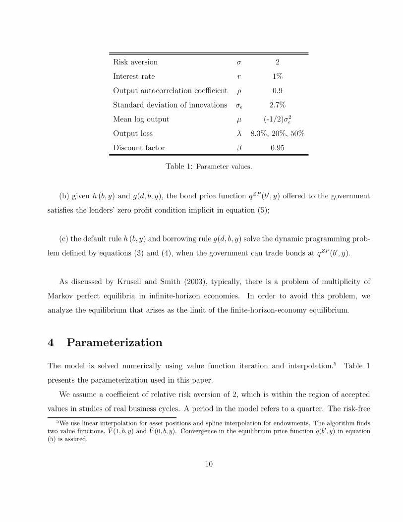
Risk aversion σ 2

Interest rate r 1%

Output autocorrelation coefficient ρ 0.9

Standard deviation of innovations σǫ 2.7%

Mean log output µ (-1/2)σ2ǫ

Output loss λ 8.3%, 20%, 50%

Discount factor β 0.95

Table 1: Parameter values.

(b) given h (b, y) and g(d, b, y), the bond price function qZP (b′, y) offered to the government

satisfies the lenders’ zero-profit condition implicit in equation (5);

(c) the default rule h (b, y) and borrowing rule g(d, b, y) solve the dynamic programming prob-

lem defined by equations (3) and (4), when the government can trade bonds at qZP (b′, y).

As discussed by Krusell and Smith (2003), typically, there is a problem of multiplicity of

Markov perfect equilibria in infinite-horizon economies. In order to avoid this problem, we

analyze the equilibrium that arises as the limit of the finite-horizon-economy equilibrium.

4 Parameterization

The model is solved numerically using value function iteration and interpolation.5 Table 1

presents the parameterization used in this paper.

We assume a coefficient of relative risk aversion of 2, which is within the region of accepted

values in studies of real business cycles. A period in the model refers to a quarter. The risk-free

5We use linear interpolation for asset positions and spline interpolation for endowments. The algorithm findstwo value functions, V (1, b, y) and V (0, b, y). Convergence in the equilibrium price function q(b′, y) in equation(5) is assured.

10

interest rate is set equal to 1%. As in Hatchondo et al. (2008), the parameter values that govern

the endowment process are chosen so as to mimic the behavior of GDP in Argentina from the

fourth quarter of 1993 to the third quarter of 2001. The parameterization of the output process

is similar to the parameterization used in other studies that consider a longer sample period (see

Aguiar and Gopinath (2006)).

As in previous studies (see, for example, Aguiar and Gopinath (2006)), we assume that the

loss in output triggered by a default is represented by a function φ (y) = λy. We show that

the value of λ does not affect the main conclusion of the paper: The mean and the standard

deviation of the spread in the simulations is higher when one assumes a duration of sovereign

bonds similar to the one observed in emerging economies instead of one-quarter bonds. One may

think that high output drops in the default period are counterfactual. However, recall that for

tractability, we are modeling all cost of defaulting as a one-period output loss. As explained

in Hatchondo et al. (2007), when it is not assumed that defaulting countries are excluded from

capital markets, assuming that the output loss triggered by a default could last more than one

period would increase the dimensionality of the state space. Hatchondo et al. (2007) show that

whether it is assumed that the output loss occurs in one period or for a stochastic number of

periods does not appear to affect the predictions of a baseline model of sovereign default.

The discount factor we assume is relatively low but higher than what is assumed in previous

studies with a cost of defaulting similar to the one assumed in this paper (for instance, Aguiar and

Gopinath (2006) assume β = 0.8). Low discount factors may be a result of political polarization

in emerging economies (see Amador (2003) and Cuadra and Sapriza (2008)).

First, we present results for two values of δ. When δ = 1, bonds have a duration of one

quarter, which is the case analyzed in previous studies. When δ = 0.053125, bonds have a

duration of four years if future coupon payments are discounted at the risk-free rate r (the

duration would be 3.66 years if future coupon payments were discounted using the average yield

implicit in bond prices observed in equilibrium). Cruces et al. (2002) report that the average

duration of Argentinean bonds included in the EMBI index was 4.13 years in 2000. This number

is not significantly different from what is observed in other emerging economies. Using a sample

of 27 emerging economies, Cruces et al. (2002) find an average duration of 4.77 years with a

11

standard deviation of 1.52. In Section 6, we show that the mean and the standard deviation of

the spread in our simulations increase monotonically with the debt duration.

5 Results

This section discusses the ability of the model to replicate some stylized facts about the macroe-

conomic behavior of emerging economies. We simulate the model for a number of periods that

allows us to extract 500 samples of 32 consecutive periods before a default. Except for the

computation of default frequencies, which are computed using all the simulation data, we fo-

cus on samples of 32 periods because we want to compare the artificial data generated by the

model with Argentine data from the fourth quarter of 1993 to the third quarter of 2001. This

is the same period that is considered in Hatchondo et al. (2008). The macroeconomic behavior

observed over that period displays the same qualitative features that can be observed using a

longer sample period or using data from other emerging markets (see, for example, Aguiar and

Gopinath (2007), Neumeyer and Perri (2005), and Uribe and Yue (2006)). The only exception is

that in the period we consider, the volatility of consumption is slightly lower than the volatility

of income, while emerging market economies tend to display a higher volatility of consumption

relative to income. In order to facilitate the comparison of simulation results with the data, we

only consider simulation sample paths where the last default was declared at least two periods

before the beginning of each sample.

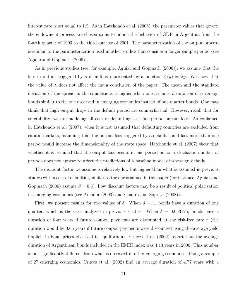
Table 2 reports moments in the data and in our simulations.6 The moments reported in the

table are chosen so as to evaluate the ability of the model to replicate distinctive business cycle

properties of emerging economies. Relative to developed economies, emerging economies feature

higher, more volatile and countercyclical interest rates; higher volatility of consumption relative

to income; and more countercyclical net exports. The trade balance (TB) is expressed as a

fraction of output (Y ). The interest rate spread (Rs) represents the margin of extra yield over

6The data for output, consumption, and trade balance was obtained from the Argentinean Finance Ministry.The spread before the first quarter of 1998 is taken from Neumeyer and Perri (2005), and from the EMBI Globalafter that.

12

the risk-free rate and is expressed in annual terms.7 The logarithm of income and consumption

are denoted by y and c, respectively. The standard deviation of x is denoted by σ (x) and is

reported in percentage terms. The correlation between x and z is denoted by ρ (x, z). Moments

are computed using detrended series. Trends are found using the Hodrick-Prescott filter with a

smoothing parameter of 1, 600.

λ = 8.3% λ = 20% λ = 50%

data 1Q 4Y 1Q 4Y 1Q 4Y

σ(y) 3.17 3.15 3.07 3.08 3.09 3.11 3.10

σ(c) 2.98 3.24 3.14 3.27 3.26 3.63 3.51

σ (TB/Y ) 1.35 0.17 0.12 0.38 0.27 0.86 0.60

σ (Rs) 2.51 0.03 0.23 0.04 0.25 0.06 0.29

ρ (c, y) 0.97 1.00 1.00 0.99 1.00 0.98 0.99

ρ (TB/Y, y) -0.69 -0.46 -0.56 -0.48 -0.57 -0.51 -0.62

ρ (Rs, y) -0.65 -0.94 -0.86 -0.86 -0.88 -0.77 -0.87

ρ (Rs, TB/Y ) 0.56 0.73 0.81 0.86 0.84 0.93 0.88

E(Rs) 7.44 0.11 2.54 0.11 2.46 0.12 2.30

debt/output 0.075 0.085 0.18 0.20 0.45 0.50

defaults per 100 years 0.12 2.56 0.11 2.44 0.12 2.32

Table 2: Business cycle statistics. The second column is computed using data from Argentina from1993 to 2001. Other columns report the mean value of each moment over 500 simulation samples foreconomies where the government issue bonds with a duration of one quarter (1Q) or four years (4Y).

Table 2 shows that the mean annual spread and the spread volatility are higher with four-

year bonds than with one-quarter bonds. It also shows that introducing four-year bonds does not

damage the ability of the model to replicate other features of the data: Other statistics reported

7Let r∗ denote the per-period constant yield implied by a bond price qZP (b′, y), namely

r∗ =1

qZP (b′, y)− δ.

The annualized spread is given by Rs =(

1+r∗

1+r

)4

− 1.

13

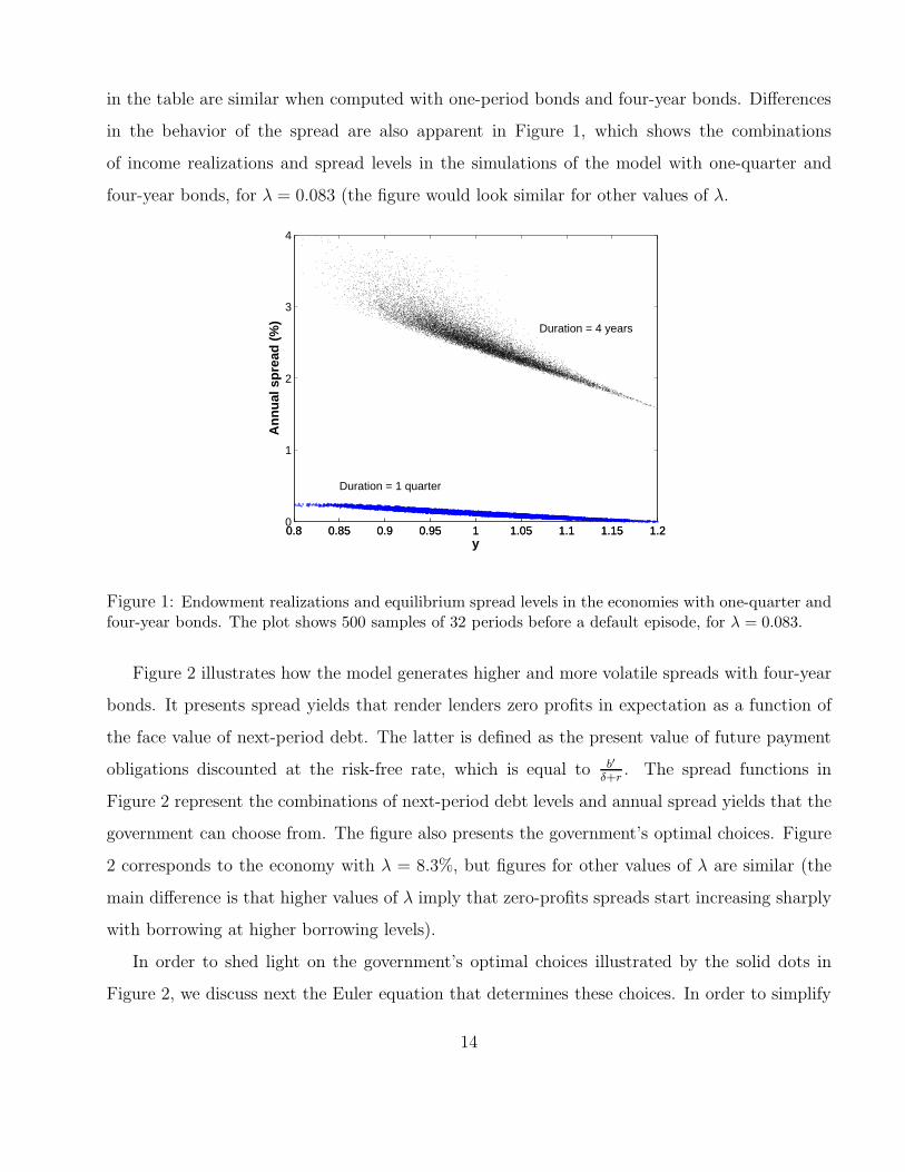
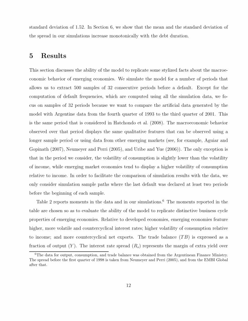
in the table are similar when computed with one-period bonds and four-year bonds. Differences

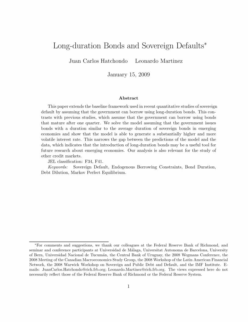
in the behavior of the spread are also apparent in Figure 1, which shows the combinations

of income realizations and spread levels in the simulations of the model with one-quarter and

four-year bonds, for λ = 0.083 (the figure would look similar for other values of λ.

0.8 0.85 0.9 0.95 1 1.05 1.1 1.15 1.20

1

2

3

4

y

An

nu

al s

pre

ad (

%)

Duration = 1 quarter

Duration = 4 years

0.8 0.85 0.9 0.95 1 1.05 1.1 1.15 1.2

Figure 1: Endowment realizations and equilibrium spread levels in the economies with one-quarter andfour-year bonds. The plot shows 500 samples of 32 periods before a default episode, for λ = 0.083.

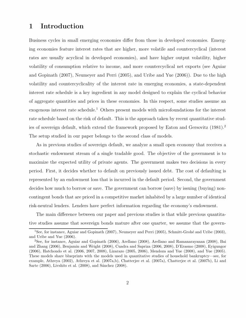
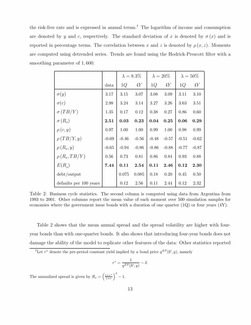
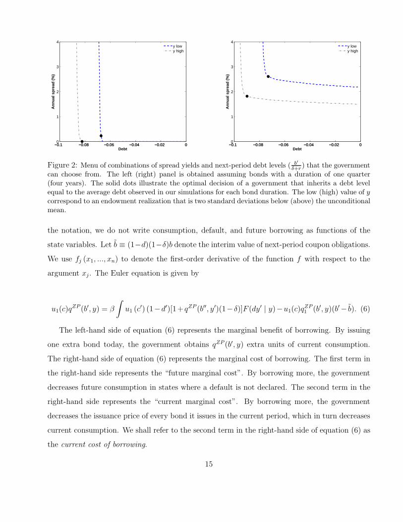
Figure 2 illustrates how the model generates higher and more volatile spreads with four-year

bonds. It presents spread yields that render lenders zero profits in expectation as a function of

the face value of next-period debt. The latter is defined as the present value of future payment

obligations discounted at the risk-free rate, which is equal to b′

δ+r. The spread functions in

Figure 2 represent the combinations of next-period debt levels and annual spread yields that the

government can choose from. The figure also presents the government’s optimal choices. Figure

2 corresponds to the economy with λ = 8.3%, but figures for other values of λ are similar (the

main difference is that higher values of λ imply that zero-profits spreads start increasing sharply

with borrowing at higher borrowing levels).

In order to shed light on the government’s optimal choices illustrated by the solid dots in

Figure 2, we discuss next the Euler equation that determines these choices. In order to simplify

14

−0.1 −0.08 −0.06 −0.04 −0.02 00

1

2

3

4

Debt

An

nu

al s

pre

ad (

%)

−0.1 −0.08 −0.06 −0.04 −0.02 0

y lowy high

−0.1 −0.08 −0.06 −0.04 −0.02 00

1

2

3

4

Debt

An

nu

al s

pre

ad (

%)

−0.1 −0.08 −0.06 −0.04 −0.02 0

y lowy high

Figure 2: Menu of combinations of spread yields and next-period debt levels ( b′

δ+r) that the government

can choose from. The left (right) panel is obtained assuming bonds with a duration of one quarter(four years). The solid dots illustrate the optimal decision of a government that inherits a debt levelequal to the average debt observed in our simulations for each bond duration. The low (high) value of y

correspond to an endowment realization that is two standard deviations below (above) the unconditionalmean.

the notation, we do not write consumption, default, and future borrowing as functions of the

state variables. Let b ≡ (1−d)(1−δ)b denote the interim value of next-period coupon obligations.

We use fj (x1, ..., xn) to denote the first-order derivative of the function f with respect to the

argument xj . The Euler equation is given by

u1(c)qZP (b′, y) = β

∫

u1 (c′) (1−d′)[1+ qZP (b′′, y′)(1−δ)]F (dy′ | y)−u1(c)qZP1 (b′, y)(b′− b). (6)

The left-hand side of equation (6) represents the marginal benefit of borrowing. By issuing

one extra bond today, the government obtains qZP (b′, y) extra units of current consumption.

The right-hand side of equation (6) represents the marginal cost of borrowing. The first term in

the right-hand side represents the “future marginal cost”. By borrowing more, the government

decreases future consumption in states where a default is not declared. The second term in the

right-hand side represents the “current marginal cost”. By borrowing more, the government

decreases the issuance price of every bond it issues in the current period, which in turn decreases

current consumption. We shall refer to the second term in the right-hand side of equation (6) as

the current cost of borrowing.

15

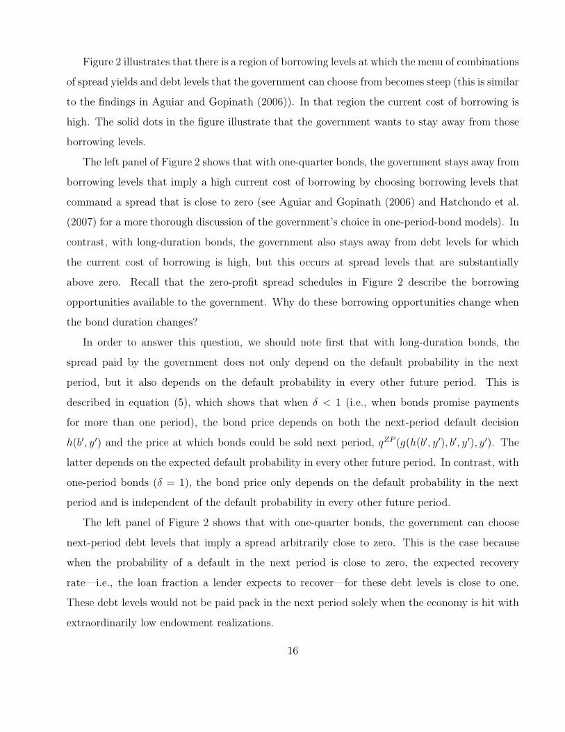
Figure 2 illustrates that there is a region of borrowing levels at which the menu of combinations

of spread yields and debt levels that the government can choose from becomes steep (this is similar

to the findings in Aguiar and Gopinath (2006)). In that region the current cost of borrowing is

high. The solid dots in the figure illustrate that the government wants to stay away from those

borrowing levels.

The left panel of Figure 2 shows that with one-quarter bonds, the government stays away from

borrowing levels that imply a high current cost of borrowing by choosing borrowing levels that

command a spread that is close to zero (see Aguiar and Gopinath (2006) and Hatchondo et al.

(2007) for a more thorough discussion of the government’s choice in one-period-bond models). In

contrast, with long-duration bonds, the government also stays away from debt levels for which

the current cost of borrowing is high, but this occurs at spread levels that are substantially

above zero. Recall that the zero-profit spread schedules in Figure 2 describe the borrowing

opportunities available to the government. Why do these borrowing opportunities change when

the bond duration changes?

In order to answer this question, we should note first that with long-duration bonds, the

spread paid by the government does not only depend on the default probability in the next

period, but it also depends on the default probability in every other future period. This is

described in equation (5), which shows that when δ < 1 (i.e., when bonds promise payments

for more than one period), the bond price depends on both the next-period default decision

h(b′, y′) and the price at which bonds could be sold next period, qZP (g(h(b′, y′), b′, y′), y′). The

latter depends on the expected default probability in every other future period. In contrast, with

one-period bonds (δ = 1), the bond price only depends on the default probability in the next

period and is independent of the default probability in every other future period.

The left panel of Figure 2 shows that with one-quarter bonds, the government can choose

next-period debt levels that imply a spread arbitrarily close to zero. This is the case because

when the probability of a default in the next period is close to zero, the expected recovery

rate—i.e., the loan fraction a lender expects to recover—for these debt levels is close to one.

These debt levels would not be paid pack in the next period solely when the economy is hit with

extraordinarily low endowment realizations.

16

In contrast, the right panel of Figure 2 shows that with four-year bonds, even if the govern-

ment chooses a next-period debt level that is arbitrarily close to zero, the discount in the bond

price would reflect a default premium substantially higher than zero. It is still true that when

the next-period debt is close to zero, the probability of a default in the next period is negligible.

However, equilibrium default probabilities in other future periods are significantly away from

zero and, therefore, the expected recovery rate on current issuances is significantly lower than

one. Suppose for example that an emerging economy is issuing long-duration debt for the first

time. No matter how small the first issuance is, lenders would anticipate an expected recovery

rate lower than one because they would know that the government would continue to issue debt

in the future. This implies that the emerging economy does not have the choice to issue small

amounts of debts at the risk-free rate.8 For any given next-period default probability (includ-

ing zero), the higher the default probabilities in other future periods, the higher the spread the

government pays in the current period.

As one would expect, default probabilities are higher—and, therefore, spreads are higher—

when we assume long-duration bonds. The literature on debt dilution discusses how credit risk

and a government’s inability to commit to future borrowing levels imply that the government

has incentives to overborrow and, therefore, to pay higher spreads.9 An increase in the current

borrowing level raises the default probability on all outstanding debt, and thus, it decreases

the market value of debt—debt dilution occurs. When issuing bonds, the government only

internalizes as a cost the dilution of the value of current bond issuances, but it does not internalize

as a cost the dilution of the value of bonds issued in past periods. In the model with one-period

bonds, when the government decides its current borrowing level, the outstanding debt level is

zero, either because the government has honored its debt obligations at the beginning of the

period or because it has defaulted on them. Thus, with one-period bonds, the government does

not have the option to dilute previously issued debt. The introduction of long-duration bonds

8This finding resembles the result in environments where the borrower does not have within-period commitmentto exclusive borrowing contracts (see, for example, Bizer and DeMarzo (1992) and Hatchondo and Martinez(2007))

9See, for instance, Bi (2006), Bizer and DeMarzo (1992), Detragiache (1994), Hatchondo and Martinez (2007),Kletzer (1984), Sachs and Cohen (1982), and Tirole (2002).

17

incorporates into the model the incentives to overborrow discussed in the literature about debt

dilution, which in turn induce the government to pay higher spreads.

Equation (6) shows that the introduction of long-duration bonds reduces the fraction of debt

that would need to be rolled over in a given period in order to keep the debt level constant (this

fraction is equal to δ). This tends to reduce the current cost of borrowing by decreasing current

issuances (b′ − b in equation (6)). With one-quarter bonds, the government has to pay back

its entire debt stock in every period it does not default, which leads to relatively high issuance

volumes. In contrast, with four-year bonds, the government only rolls over a small fraction of

its debt, and therefore, the decrease in the issuance price in the current cost of borrowing is

weighted by a smaller number (a smaller issuance volume).

Next, we discuss why introducing long-duration bonds allows the model to generate a higher

spread volatility. Figure 2 shows that with four-year bonds, the menu of interest rates available

to the government is more sensitive to the current endowment realization than with one-period

bonds. This is the case because lower income levels today imply lower expected income levels in

future periods, and thus, lenders anticipate higher default probabilities in future periods (recall

that with long-duration bonds, the interest rate spread depends on default probabilities in every

future period, not just in the next period). When four-year bonds are assumed, the higher

sensitivity of the menu of zero-profit interest rates to the endowment leads the government to

accept spread levels that are more sensitive to income (see the dots in Figure 2) and, thus, it

leads to a higher spread volatility.

Table 2 illustrates how equilibrium debt levels generated by the model are close to the cost of

defaulting. For instance, if we assume that the cost of defaulting is 50% of output, the mean debt

level generated by the model is close to 50% of output. Thus, independently from the assumed

debt duration, the debt level generated by the model can be increased by increasing value of

λ. We do not parameterize the model to replicate debt levels in the data. The reason for this

is that debt levels generated by the baseline model of sovereign default are difficult to compare

with debt levels in the data. In the model, the government cannot borrow and save at the same

time, the recovery rate on debt in default is zero, and all debt is held by foreigners.

Table 2 also shows that the face value of debt is higher with four-year bonds than with one-

18

quarter bonds. There are two reasons for this. First, as explained before, the government is only

concerned about the effect of current-period issuances on the price of these issuances, which,

with long-duration bonds, constitute a small fraction of the total debt level. This induces the

government to choose a higher debt burden with long-duration bonds. Second, for any given

debt burden, the higher default probability obtained with long-duration bonds implies a higher

face value of debt. The existence of scenarios in which the government will default implies that

the actual debt burden is lower than the face value of future coupon obligations. For a given

debt burden, a higher default probability implies a higher face value of debt.

It should also be mentioned that the introduction of long-duration bonds could allow models

of sovereign default to explain both debt levels and debt service levels observed in the data at

the same time. With one-period bonds, debt levels are very close to debt service levels. On the

one hand, studies that target debt service levels generate debt levels that are too low compared

with the data. On the other hand, studies that target debt levels generate debt service levels

that are too high compared with the data. With long-duration bonds, if the bond duration in

the model matches the one in the data, and the spread in the model matches the spread in the

data, targeting the mean debt level is equivalent to targeting the mean debt service level.

In addition, Table 2 shows that the mean annual spread in percentage terms generated by the

model, is almost identical to the number of defaults per 100 years. Recall that bond values are

determined by risk-neutral lenders, and the recovery rate in case of default is zero. Measuring the

default probability in the data using historical default frequencies is difficult. Default episodes

are low frequency events and, therefore, a large sample size would be necessary to obtain precise

estimates of the default probability. Furthermore, there are disagreements about what constitutes

a sovereign default, and the default probability may change over time due to changes in the

structure of international capital markets, changes in the probability distribution of shocks that

hit the economy, etc. For instance, the environment under which Argentina borrowed from

international markets and the tradeoffs involved in a default decision during the last two decades

might have been quite different from the environment 200 years ago.

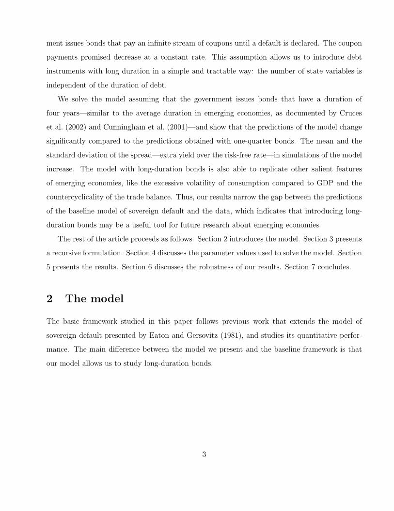
We also find that the expected utility of domestic agents in decreasing with respect to the

bond-duration. Figure 3 illustrates the consumption compensation that would make domestic

19

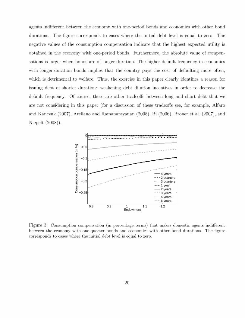
agents indifferent between the economy with one-period bonds and economies with other bond

durations. The figure corresponds to cases where the initial debt level is equal to zero. The

negative values of the consumption compensation indicate that the highest expected utility is

obtained in the economy with one-period bonds. Furthermore, the absolute value of compen-

sations is larger when bonds are of longer duration. The higher default frequency in economies

with longer-duration bonds implies that the country pays the cost of defaulting more often,

which is detrimental to welfare. Thus, the exercise in this paper clearly identifies a reason for

issuing debt of shorter duration: weakening debt dilution incentives in order to decrease the

default frequency. Of course, there are other tradeoffs between long and short debt that we

are not considering in this paper (for a discussion of these tradeoffs see, for example, Alfaro

and Kanczuk (2007), Arellano and Ramanarayanan (2008), Bi (2006), Broner et al. (2007), and

Niepelt (2008)).

0.8 0.9 1 1.1 1.2

−0.25

−0.2

−0.15

−0.1

−0.05

0

Endowment

Con

sum

ptio

n co

mpe

nsat

ion

(in %

)

4 years2 quarters3 quarters1 year2 years3 years5 years6 years

Figure 3: Consumption compensation (in percentage terms) that makes domestic agents indifferentbetween the economy with one-quarter bonds and economies with other bond durations. The figurecorresponds to cases where the initial debt level is equal to zero.

20

6 Robustness

This paper wants to convey that, other things being equal, one should expect a model to generate

higher spreads and higher spread volatilities with bonds of longer duration. Of course, there are

other mechanisms that can increase spreads and spread volatilities in these models. In this

section, we discuss how the message we want to convey is robust to changes in our assumptions.

In order to do so, we present robustness exercises, and we discuss results in related work.

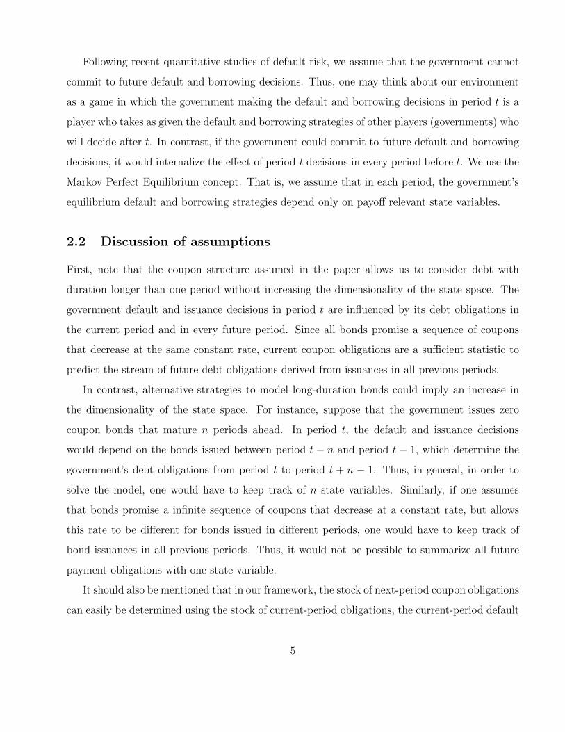
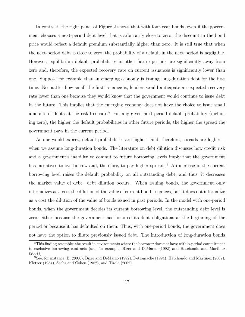
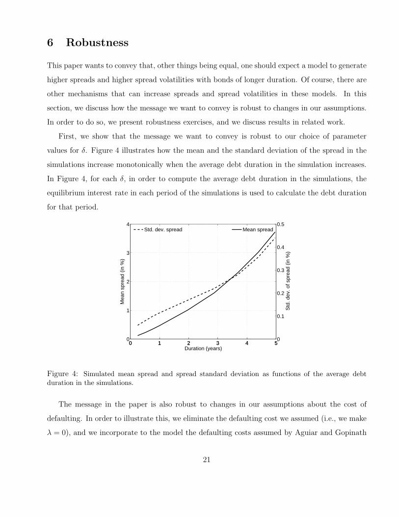
First, we show that the message we want to convey is robust to our choice of parameter

values for δ. Figure 4 illustrates how the mean and the standard deviation of the spread in the

simulations increase monotonically when the average debt duration in the simulation increases.

In Figure 4, for each δ, in order to compute the average debt duration in the simulations, the

equilibrium interest rate in each period of the simulations is used to calculate the debt duration

for that period.

0 1 2 3 4 50

1

2

3

4

Duration (years)

Mea

n sp

read

(in

%)

0 1 2 3 4 50

0.1

0.2

0.3

0.4

0.5

Std

. dev

. of s

prea

d (in

%)

Std. dev. spread Mean spread

Figure 4: Simulated mean spread and spread standard deviation as functions of the average debtduration in the simulations.

The message in the paper is also robust to changes in our assumptions about the cost of

defaulting. In order to illustrate this, we eliminate the defaulting cost we assumed (i.e., we make

λ = 0), and we incorporate to the model the defaulting costs assumed by Aguiar and Gopinath

21

(2006): i) the country is excluded from capital markets in the default period and, in subsequent

periods, faces a probability of reentry to capital markets equal to 10%, and ii) the country loses

2% of its endowment in each period it remains excluded from capital markets. We solve the

modified model, and find that the mean spread in the simulations increased from 0.04% in the

economy with one-quarter bonds to 0.74% in the economy with four-year bonds (these statistics

are computed exactly as those reported in Table 2, but with the additional restriction that the

chosen samples do not contain periods where the country is excluded from capital markets).

These mean spread levels are around a third of the values presented in Table 2, both for one-

quarter and four-year bonds. That is, the mean spread is still almost twenty times higher with

four-year bonds than with one-quarter bonds. The spread standard deviation in the simulations

increased from 0.008 in the economy with one-quarter bonds to 0.06 in the economy with four-

year bonds. These values are around a fourth of the ones presented in Table 2. As discussed

below, the level of the increase in the mean and the standard deviation of the spread that can

be obtained by assuming longer bonds depends on the sensitivity of the cost of defaulting to the

shock in the model.

The low mean spread level with one-period bonds that we report in table 2 is observed in most

studies of sovereign default. For instance, Aguiar and Gopinath (2006) report spread levels similar

to the ones observed in our model with one-period bonds. The low spread levels generated by the

baseline sovereign default framework motivated Guerrieri et al. (2008) to introduce production

into the model.

Arellano (2008) succeeds in presenting a quantitative model with one-period bonds that

generates a significant mean spread. This is achieved by assuming a cost of defaulting that is

more sensitive to current income than the one we assume. However, in her simulations, when

economic conditions are good, the spread generated by the model is close to zero, which is not

observed in the data. The mean spread in Arellano (2008) is close to the mean spread in the

data because when economic conditions are bad the spread in her simulations is higher than in

the data—see Figure 5 in Arellano (2008). Our findings suggests that even when the default

cost resembles the one used in Arellano (2008), introducing long-duration bonds could improve

the ability of the model to replicate the spread behavior in the data. The reason is that when

22

economic conditions are good and the next-period probability of default is small, long-duration-

bond spreads may be significantly away from zero because lenders anticipate a higher default

probability in other future periods. This is shown by Chatterjee and Eyigungor (2008), who

solve a model of sovereign default with long-duration bonds and the costs of defaulting assumed

by Arellano (2008).10 They calibrate the model to obtain an average spread of 8.8% with long-

duration bonds. They also show that with the same parameterization and one-period bonds,

the average spread in the simulations decline to 0.4%. Their results seem consistent with the

findings of Arellano and Ramanarayanan (2008). They study the optimal duration choice over

the business cycle in a sovereign default model with the cost of defaulting assumed by Arellano

(2008). The mean spread in their simulations is 6.58% for two-year bonds and 6.25% for ten-year

bonds. They do not solve the model with one-period bonds.

Mendoza and Yue (2008) study sovereign defaults in a production economy with an endoge-

nous output cost of defaulting. In their benchmark simulations, the mean spread is 2.4% (they

assume a discount factor of 0.87 for their quarterly model). They also show that if they shut

down their endogenous output cost of defaulting and replace it with the (exogenous) proportional

output cost assumed by Aguiar and Gopinath (2006), the mean spread in the simulations de-

creases to 0.5%. Mendoza and Yue (2008) explain that the decrease in the mean spread obtained

in the simulations is explained in part by the lower sensitivity of the output cost to the state

assumed by Aguiar and Gopinath (2006) (and other previous studies).

Benjamin and Wright (2008) show that a model with debt renegotiation can generate higher

spreads during the renegotiation period than in the pre-default period, as observed in the data (for

example, the average spread in Argentina during the 2001-2005 renegotiation period was 55%).

The market value of sovereign bonds decline after the sovereign declares a default. However, in

their simulations, pre-default spread levels are lower than in the data. Pouzo (2008) conducts a

similar exercise and reports an average spread of 1% for pre-default simulation samples and of

119% for renegotiation-period simulation samples.

10Chatterjee and Eyigungor (2008) show that introducing a shock the borrower’s utility function with a con-tinuous support helps solving a default model with long-duration bonds using the discrete state space techniqueand assuming a discrete support for the endowment process.

23

7 Conclusions

We presented an extended version of the baseline model of sovereign default that allows us to

study economies where the government issues long-duration bonds. We showed that when the

model is parameterized to display a bond duration similar to the one observed in the data, the

mean and the volatility of the interest rate are substantially larger than when one-quarter bonds

are assumed. Replicating the behavior of interest rates in emerging economies is an important

goal in studies of these economies. Our results narrow the gap between the predictions of the

baseline model and the data, indicating that the extended model may be a useful tool for future

research.

24

References

Aguiar, M. and Gopinath, G. (2006). ‘Defaultable debt, interest rates and the current account’.

Journal of International Economics, volume 69, 64–83.

Aguiar, M. and Gopinath, G. (2007). ‘Emerging markets business cycles: the cycle is the trend’.

Journal of Political Economy , volume 115, no. 1, 69–102.

Alfaro, L. and Kanczuk, F. (2007). ‘Debt Maturity: Is Long-Term Debt Optimal?’ NBER

Working Paper 13119.

Amador, M. (2003). ‘A Political Economy Model of Sovereign Debt Repayment’. Manuscript,

Stanford University.

Arellano, C. (2008). ‘Default Risk and Income Fluctuations in Emerging Economies’. American

Economic Review , volume 98(3), 690–712.

Arellano, C. and Ramanarayanan, A. (2008). ‘Default and the Maturity Structure in Sovereign

Bonds’. Mimeo, University of Minnesota.

Arteta, C. and Hale, G. (2008). ‘Sovereign Debt Crises and Credit to the Private Sector’. Journal

of International Economics, volume 74, 53–69.

Athreya, K. (2002). ‘Welfare Implications of the Bankruptcy Reform Act of 1999’. Journal of

Monetary Economics, volume 49, 1567–1595.

Athreya, K., Tam, X. S., and Young, E. R. (2007a). ‘Does Rising Income Risk Lead to Better

Risk Sharing?’ Manuscript, University of Virginia.

Athreya, K., Tam, X. S., and Young, E. R. (2007b). ‘A Quantitative Model of Information and

Unsecured Lending’. Manuscript, University of Virginia.

Athreya, K. B. and Janicki, H. P. (2006). ‘Credit exclusion in quantitative models of bankruptcy:

does it matter?’ Economic Quarterly , volume 92, no. 1, 17–50. Federal Reserve Bank of

Richmond.

25

Bai, Y. and Zhang, J. (2006). ‘Financial integration and international risk sharing’. Working

Paper, Michigan University.

Benjamin, D. and Wright, M. L. J. (2008). ‘Recovery Before Redemption? A Theory of Delays

in Sovereign Debt Renegotiations’. Manuscript.

Bi, R. (2006). ‘Debt Dilution and the Maturity Structure of Sovereign Bonds’. Manuscript,

University of Maryland.

Bizer, D. S. and DeMarzo, P. (1992). ‘Sequential Banking’. Journal of Political Economy , volume

100, 41–61.

Broner, F. A., Lorenzoni, G., and Schmukler, S. L. (2007). ‘Why do emerging economies borrow

short term?’ National Bureau of Economic Research Working Paper 13076.

Chatterjee, S., Corbae, D., Nakajima, M., and Rıos-Rull, J.-V. (2007a). ‘A Quantitative Theory

of Unsecured Consumer Credit with Risk of Default’. Econometrica, volume 75, 1525–1589.

Chatterjee, S., Corbae, D., and Rıos-Rull, J.-V. (2007b). ‘Credit Scoring and Competitive Pricing

of Default Risk’. Manuscript, University of Texas at Austin.

Chatterjee, S. and Eyigungor, B. (2008). ‘Maturity, Indebtedness and Default Risk’. Unpublished

manuscript.

Cole, H., Dow, J., and English, W. (1995). ‘Default, settlement, and signaling: lending resump-

tion in a reputational model of sovereign debt’. International Economic Review , volume 36,

no. 2, 365–385.

Copeland, T. E. and Weston, J. F. (1992). Financial theory and corporate policy . Addison-Wesley

Publishing Company.

Cruces, J. J., Buscaglia, M., and Alonso, J. (2002). ‘The Term Structure of Country Risk and

Valuation in Emerging Markets’. Manuscript, Universidad Nacional de La Plata.

26

Cuadra, G. and Sapriza, H. (2006). ‘Sovereign default, terms of trade, and interest rates in

emerging markets’. Working Paper 2006-01, Banco de Mexico.

Cuadra, G. and Sapriza, H. (2008). ‘Sovereign default, interest rates and political uncertainty in

emerging markets’. Journal of International Economics. Forthcoming.

Cunningham, A., Dixon, L., and Hayes, S. (2001). ‘Analyzing yield spreads on emerging market

sovereign bonds’. Financial Stability Review , volume December, 175–186.

D’Erasmo, P. (2008). ‘Government Reputation and Debt Repayment in Emerging Economies’.

Manuscript, University of Texas at Austin.

Detragiache, E. (1994). ‘Sensible buybacks of sovereign debt’. Journal of Development Eco-

nomics , volume 43, 317–333.

Eaton, J. and Gersovitz, M. (1981). ‘Debt with potential repudiation: theoretical and empirical

analysis’. Review of Economic Studies , volume 48, 289–309.

Eichengreen, B. and Portes, R. (2000). ‘Debt Restructuring With and Without the IMF’.

Manuscript, UC Berkeley.

Eyigungor, B. (2006). ‘Sovereign Debt Spreads in a Markov Switching Regime’. Manuscript,

UCLA.

Gelos, G., Sahay, R., and Sandleris, G. (2004). ‘Sovereign Borrowing by Developing Countries:

What Determines Market Access?’ IMF Working Paper 04/221.

Guerrieri, V., Lorenzoni, G., and Perri, F. (2008). ‘International Borrowing, Investment and

Default’. Manuscript.

Hatchondo, J. C. and Martinez, L. (2007). ‘Credit risk without commitment’. Manuscript.

Federal Reserve Bank of Richmond.

Hatchondo, J. C., Martinez, L., and Sapriza, H. (2006). ‘Computing business cycles in emerging

economy models’. Working Paper No. 06-11. Federal Reserve Bank of Richmond.

27

Hatchondo, J. C., Martinez, L., and Sapriza, H. (2007). ‘Quantitative Models of Sovereign

Default and the Threat of Financial Exclusion’. Economic Quarterly , volume 93, 251–286.

No. 3.

Hatchondo, J. C., Martinez, L., and Sapriza, H. (2008). ‘Heterogeneous borrowers in quantitative

models of sovereign default.’ International Economic Review . Forthcoming.

IMF (2002). ‘Sovereign Debt Restructurings and the Domestic Economy Experience in Four

Resent Cases’. Policy development and review department.

Kaminsky, G. and Reinhart, C. M. (1999). ‘The Twin Crises: The Causes of Banking and

Balance of Payments Crises’. American Economic Review , volume 89, 473–500.

Kletzer, K. M. (1984). ‘Asymmetries of Information and LDC Borrowing with Sovereign Risk’.

The Economic Journal , volume 94, 287–307.

Kobayashi, K. (2006). ‘Payment uncertainty, the division of labor, and productivity declines in

great depressions’. Review of Economic Dynamics , volume 9, 715–741.

Krusell, P. and Smith, A. (2003). ‘Consumption-savings decisions with quasi-geometric discount-

ing’. Econometrica, volume 71, no. 1, 365–375.

Kumhof, M. (2004). ‘Fiscal crisis resolution: taxation versus inflation’. Manuscript, Stanford

University.

Kumhof, M. and Tanner, E. (2005). ‘Government Debt: A Key Role in Financial Intermediation’.

IMF Working Paper 05/57.

Li, W. and Sarte, P.-D. (2006). ‘U.S. consumer bankruptcy choice: The importance of general

equilibrium effects’. Journal of Monetary Economics, volume 53, 613–631.

Livshits, I., MacGee, J., and Tertilt, M. (2008). ‘Consumer Bankruptcy: A Fresh Start,’. Amer-

ican Economic Review . Forthcoming.

28

Lizarazo, S. (2005). ‘Sovereign risk and risk averse international investors’. Working Paper,

ITAM.

Lizarazo, S. (2006). ‘Contagion of financial crises in sovereign debt markets’. Working Paper,

ITAM.

Mendoza, E. and Yue, V. (2008). ‘A Solution to the Default Risk-Business Cycle Disconnect’.

Manuscript, New York University.

Meyersson, E. (2006). ‘Debt intolerance and institutions, an empirical investigation into the

institutional effect of sovereign debt’.

Neumeyer, P. and Perri, F. (2005). ‘Business cycles in emerging economies: the role of interest

rates’. Journal of Monetary Economics, volume 52, 345–380.

Niepelt, D. (2008). ‘Debt Maturity without Commitment’. Manuscript, Study Center Gerzensee.

Pouzo, D. (2008). ‘Optimal Taxation With Endogenous Default Under Incomplete Markets’.

Manuscript, NYU.

Sachs, J. and Cohen, D. (1982). ‘LDC borrowing with default risk’. National Bureau of Economic

Research Working Paper 925.

Sanchez, J. M. (2008). ‘The Role of Information in Consumer Debt and Bankruptcy’. Manuscript,

University of Rochester.

Sandleris, G. (2006). ‘Sovereign Defaults: Information, Investment and Credit’. Manuscript,

Johns Hopkins.

Schmitt-Grohe, S. and Uribe, M. (2003). ‘Closing small open economy models’. Journal of

International Economics, volume 61, 163–185.

Tirole, J. (2002). ‘Financial Crises, Liquidity, and the International Monetary System’. Princeton

University Press.

29

Uribe, M. and Yue, V. (2006). ‘Country spreads and emerging countries: Who drives whom?’

Journal of International Economics, volume 69, 6–36.

Wright, M. L. J. (2002). ‘Reputations and Sovereign Debt’. Manuscript, Stanford University.

Wright, M. L. J. (2005). ‘Coordinating Creditors’. The American Economic Review, Papers and

Proceedings , volume 95, no. 2, 388–392.

Yue, V. (2005). ‘Sovereign default and debt renegotiation’. Working Paper, NYU.

30