Logic programming: laxness and saturation✩

Ekaterina Komendantskaya∗

Department of Computer Science, Heriot-Watt University, Edinburgh, UK

John Power∗

Department of Computer Science, University of Bath, BA2 7AY, UK

Abstract

A propositional logic program P may be identified with a PfPf -coalgebra onthe set of atomic propositions in the program. The corresponding C(PfPf )-coalgebra, where C(PfPf ) is the cofree comonad on PfPf , describes derivationsby resolution. That correspondence has been developed to model first-orderprograms in two ways, with lax semantics and saturated semantics, based on lo-cally ordered categories and right Kan extensions respectively. We unify the twoapproaches, exhibiting them as complementary rather than competing, reflect-ing the theorem-proving and proof-search aspects of logic programming. Whilemaintaining that unity, we further refine lax semantics to give finitary modelsof logic programs with existential variables, and to develop a precise semanticrelationship between variables in logic programming and worlds in local state.

Keywords: Logic programming, coalgebra, coinductive derivation tree,Lawvere theories, lax transformations, saturation

1. Introduction

Over recent years, there has been a surge of interest in category theoreticsemantics of logic programming. Research has focused on two ideas: lax seman-tics, proposed by the current authors and collaborators [1], and saturated se-mantics, proposed by Bonchi and Zanasi [2]. Both ideas are based on coalgebra,agreeing on variable-free logic programs. Both ideas use subtle, well-establishedcategory theory, associated with locally ordered categories and with right Kanextensions respectively [3]. And both elegantly clarify and extend establishedlogic programming constructs and traditions, for instance [4] and [5].

✩No data was generated in the course of this research.∗Corresponding authorEmail addresses: ek19@hw.ac.uk (Ekaterina Komendantskaya), A.J.Power@bath.ac.uk

(John Power)

Preprint submitted to Elsevier July 19, 2018

brought to you by COREView metadata, citation and similar papers at core.ac.uk

provided by Heriot Watt Pure

Until now, the two ideas have been presented as alternatives, competing witheach other rather than complementing each other. A central thesis of this paperis that the competition is illusory, the two ideas being two views of a single, ele-gant body of theory, those views reflecting different but complementary aspectsof logic programming, those aspects broadly corresponding with the notions oftheorem proving and proof search. Such reconciliation has substantial conse-quences. In particular, it means that whenever one further refines one approach,as we shall do to the original lax approach in two substantial ways here, oneshould test whether the proposed refinement also applies to the other approach,and see what consequences it has from the latter perspective.

The category theoretic basis for both lax and saturated semantics is as fol-lows. It has long been observed, e.g., in [6, 7], that logic programs inducecoalgebras, allowing coalgebraic modelling of their operational semantics. Us-ing the definition of logic program in Lloyd’s book [8], given a set of atoms At,one can identify a variable-free logic program P built over At with a PfPf -coalgebra structure on At, where Pf is the finite powerset functor on Set: eachatom is the head of finitely many clauses in P , and the body of each clausecontains finitely many atoms. It was shown in [9] that if C(PfPf ) is the cofreecomonad on PfPf , then, given a logic program P qua PfPf -coalgebra, the corre-sponding C(PfPf )-coalgebra structure characterises the and-or derivation treesgenerated by P , cf. [4]. That fact has formed the basis for our work on laxsemantics [1, 10, 11, 12, 13] and for Bonchi and Zanasi’s work on saturationsemantics [14, 2].

In attempting to extend the analysis to arbitrary logic programs, both groupsfollowed the tradition of [15, 6, 5, 16]: given a signature Σ of function symbols,let LΣ denote the Lawvere theory generated by Σ, and, given a logic program Pwith function symbols in Σ, consider the functor category [Lop

Σ , Set], extendingthe set At of atoms in a variable-free logic program to the functor from Lop

Σ toSet sending a natural number n to the set At(n) of atomic formulae with at mostn variables generated by the function symbols in Σ and the predicate symbols inP . We all sought to model P by a [Lop

Σ , PfPf ]-coalgebra p : At −→ PfPfAt that,at n, takes an atomic formula A(x1, . . . , xn) with at most n variables, considersall substitutions of clauses in P into clauses with variables among x1, . . . , xn

whose head agrees with A(x1, . . . , xn), and gives the set of sets of atomic formu-lae in antecedents, naturally extending the construction for variable-free logicprograms. However, that idea is too simple for two reasons. We all dealt withthe second problem in the same way, so we shall discuss it later, but the firstproblem is illustrated by the following example.

Example 1. ListNat (for lists of natural numbers) denotes the logic program1. nat(0)←2. nat(s(x))← nat(x)3. list(nil)←4. list(cons(x, y))← nat(x), list(y)

ListNat has nullary function symbols 0 and nil, a unary function symbol s,

2

and a binary function symbol cons. So the signature Σ of ListNat contains fourelements.

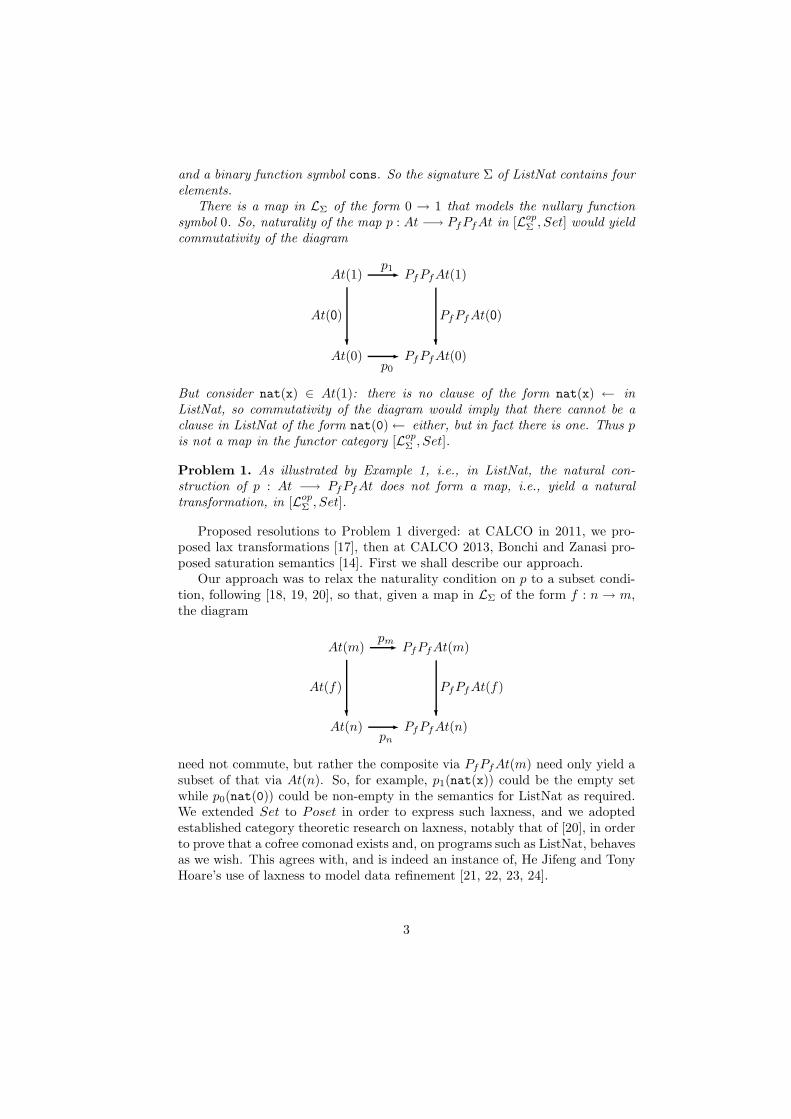
There is a map in LΣ of the form 0 → 1 that models the nullary functionsymbol 0. So, naturality of the map p : At −→ PfPfAt in [Lop

Σ , Set] would yieldcommutativity of the diagram

At(1)p1✲ PfPfAt(1)

At(0)

At(0)

❄

p0

✲ PfPfAt(0)

PfPfAt(0)

❄

But consider nat(x) ∈ At(1): there is no clause of the form nat(x) ← inListNat, so commutativity of the diagram would imply that there cannot be aclause in ListNat of the form nat(0)← either, but in fact there is one. Thus pis not a map in the functor category [Lop

Σ , Set].

Problem 1. As illustrated by Example 1, i.e., in ListNat, the natural con-struction of p : At −→ PfPfAt does not form a map, i.e., yield a naturaltransformation, in [Lop

Σ , Set].

Proposed resolutions to Problem 1 diverged: at CALCO in 2011, we pro-posed lax transformations [17], then at CALCO 2013, Bonchi and Zanasi pro-posed saturation semantics [14]. First we shall describe our approach.

Our approach was to relax the naturality condition on p to a subset condi-tion, following [18, 19, 20], so that, given a map in LΣ of the form f : n → m,the diagram

At(m)pm✲ PfPfAt(m)

At(n)

At(f)

❄

pn

✲ PfPfAt(n)

PfPfAt(f)

❄

need not commute, but rather the composite via PfPfAt(m) need only yield asubset of that via At(n). So, for example, p1(nat(x)) could be the empty setwhile p0(nat(0)) could be non-empty in the semantics for ListNat as required.We extended Set to Poset in order to express such laxness, and we adoptedestablished category theoretic research on laxness, notably that of [20], in orderto prove that a cofree comonad exists and, on programs such as ListNat, behavesas we wish. This agrees with, and is indeed an instance of, He Jifeng and TonyHoare’s use of laxness to model data refinement [21, 22, 23, 24].

3

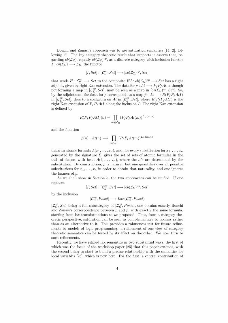
Bonchi and Zanasi’s approach was to use saturation semantics [14, 2], fol-lowing [6]. The key category theoretic result that supports it asserts that, re-garding ob(LΣ), equally ob(LΣ)op, as a discrete category with inclusion functorI : ob(LΣ) −→ LΣ, the functor

[I, Set] : [LopΣ , Set] −→ [ob(LΣ)op, Set]

that sends H : LopΣ −→ Set to the composite HI : ob(LΣ)op −→ Set has a right

adjoint, given by right Kan extension. The data for p : At −→ PfPfAt, althoughnot forming a map in [Lop

Σ , Set], may be seen as a map in [ob(LΣ)op, Set]. So,by the adjointness, the data for p corresponds to a map p̄ : At −→ R(PfPfAtI)in [Lop

Σ , Set], thus to a coalgebra on At in [LopΣ , Set], where R(PfPfAtI) is the

right Kan extension of PfPfAtI along the inclusion I. The right Kan extensionis defined by

R(PfPfAtI)(n) =∏

m∈LΣ

(PfPfAt(m))LΣ(m,n)

and the function

p̄(n) : At(n) −→∏

m∈LΣ

(PfPfAt(m))LΣ(m,n)

takes an atomic formula A(x1, . . . , xn), and, for every substitution for x1, . . . , xn

generated by the signature Σ, gives the set of sets of atomic formulae in thetails of clauses with head A(t1, . . . , tn), where the ti’s are determined by thesubstitution. By construction, p̄ is natural, but one quantifies over all possiblesubstitutions for x1, . . . , xn in order to obtain that naturality, and one ignoresthe laxness of p.

As we shall show in Section 5, the two approaches can be unified. If onereplaces

[I, Set] : [LopΣ , Set] −→ [ob(LΣ)op, Set]

by the inclusion[Lop

Σ , Poset] −→ Lax(LopΣ , Poset)

[LopΣ , Set] being a full subcategory of [Lop

Σ , Poset], one obtains exactly Bonchiand Zanasi’s correspondence between p and p̄, with exactly the same formula,starting from lax transformations as we proposed. Thus, from a category the-oretic perspective, saturation can be seen as complementary to laxness ratherthan as an alternative to it. This provides a robustness test for future refine-ments to models of logic programming: a refinement of one view of categorytheoretic semantics can be tested by its effect on the other. We now turn tosuch refinements.

Recently, we have refined lax semantics in two substantial ways, the first ofwhich was the focus of the workshop paper [25] that this paper extends, withthe second being to start to build a precise relationship with the semantics forlocal variables [26], which is new here. For the first, a central contribution of

4

lax semantics has been the inspiration it provided towards the development ofan efficient logic programming algorithm [1, 10, 11, 12, 13]. That developmentdrew our attention to the semantic significance of existential variables: suchvariables do not appear in ListNat, and they are not needed for a considerablebody of logic programming, but they do appear in logic programs such as thefollowing, which is a leading example in Sterling and Shapiro’s book [27].

Example 2. GC (for graph connectivity) denotes the logic program1. connected(x, x)←2. connected(x, y)← edge(x, z), connected(z, y)

There is a variable z in the tail of the second clause of GC that does not appearin its head, whereas no such variable appears in ListNat. Such a variable is calledan existential variable, the presence of which challenges the algorithmic signifi-cance of lax semantics. In describing the putative coalgebra p : At −→ PfPfAtjust before Example 1, we referred to all substitutions of clauses in P intoclauses with variables among x1, . . . , xn whose head agrees with A(x1, . . . , xn).If there are no existential variables, that amounts to term-matching, which isalgorithmically efficient; but if existential variables do appear, the mere pres-ence of a unary function symbol generates an infinity of such substitutions,creating algorithmic difficulty, which, when first introducing lax semantics, weavoided modelling by replacing the outer instance of Pf by Pc, thus allowing forcountably many choices.

Bonchi and Zanasi, in [14, 2], followed the lead of lax semantics in usingPc rather than Pf in order to account for existential variables, but one needsa careful study to see that. In saturated semantics, countability arises in twoways: applying the right Kan extension R yields countability as there may becountably many substitutions for variables; and using Pc rather than Pf alsoyields countability. In the absence of existential variables, Bonchi and Zanasicould have applied saturation to the map p : At −→ PfPfAt, with the right Kanextension generating the countability required for saturation. However, in thepresence of existential variables, there is no such map into PfPfAt to which toapply saturation. So for saturated semantics, our analysis of existential variablesmakes for a subtle difference, clarifying where countability is required.

That is the second of the two problems mentioned just before Example 1.More succinctly, it may be expressed as follows:

Problem 2. As illustrated by Example 2, an arbitrary logic program does notgenerate a map of the form p : At −→ PfPfAt. Previous work addressed thatby an artificial use of countability.

We have long sought a solution to Problem 2. We finally found and presentedsuch a resolution in the workshop paper [25] that this paper extends. We bothrefine it a little more, as explained later, and give more detail here.

The conceptual key to the resolution was to isolate and give finitary laxsemantics to the notion of coinductive tree [28, 1]. Coinductive trees arise from

5

term-matching resolution [28, 1], which is a variant of SLD-resolution. Term-matching captures the theorem proving aspect of logic programming, whichis distinct from, but complementary with, its problem solving aspect, whichis captured by SLD-resolution [12, 11]. The difference is that in the term-matching approach, one only substitutes in a goal after having exhausted allpossible term-matching, whereas in SLD-resolution, one uses full unification atany time. We called the derivation trees arising from term-matching coinductivetrees in order to mark their connection with coalgebraic logic programming,which we also developed.

Syntactically, one can observe the difference between lax semantics and sat-uration semantics in that lax semantics models coinductive trees, which arefinitely branching, whereas saturation involves infinitely many possible substi-tutions, leading Bonchi and Zanasi to model different kinds of trees, their focusbeing on proof search rather than on theorem proving.

Chronologically, we introduced lax semantics in 2011 as above [17]; lax se-mantics inspired us to investigate term-matching and to introduce the notionof coinductive tree [28]; because of the possibility of existential variables, ourlax semantics for coinductive trees, despite inspiring the notion, was potentiallyinfinitary [1]; so we have now refined lax semantics to ensure finitariness of thesemantics for coinductive trees, even in the presence of existential variables [25],introducing it in the workshop paper that this paper extends. We further refinelax semantics here to start to build a precise relationship with the semantics oflocal variables [26], which we plan to develop further in future. We regard itas positive that lax semantics brings to the fore, in semantic terms, the signifi-cance of existential variables, and allows a precise semantic relationship betweenthe role of variables in logic programming and local variables as they arise inprogramming more generally.

The semantics we give in this paper is subtly different to that in [25]. Here,we disambiguate the role of Pf in our modelling of existential variables: inSection 6, we consider

∫At, then apply PfPf to it, whereas we mixed a con-

struction for∫

with Pf in [25], but that does not quite match the modellingof local state. We also give far more detail throughout this paper: in givingexamples, in explaining the relationship with Bonchi and Zanasi’s saturatedsemantics, in proofs, and in developing the relationship with local state.

The paper is organised as follows. In Section 2, we set logic programming ter-minology, explain the relationship between term-rewriting and SLD-resolution,and introduce the notion of coinductive tree. In Section 3, we give semanticsfor variable-free logic programs. This semantics could equally be seen as laxsemantics or saturated semantics, as they agree in the absence of variables. InSection 4, we model coinductive trees for logic programs without existentialvariables and explain the difficulty in modelling coinductive trees for arbitrarylogic programs. In Section 5, we recall saturation semantics and make precisethe relationship between it and lax semantics. We devote Section 6 of the paperto refining lax semantics, while maintaining the relationship with saturationsemantics, to model the coinductive trees generated by logic programs with ex-istential variables, and in Section 7, we start to build a precise relationship with

6

the semantics of local state [26].

2. Theorem proving in logic programming

A signature Σ consists of a set F of function symbols f, g, . . . each equippedwith an arity. Nullary (0-ary) function symbols are constants. For any set Varof variables, the set Ter(Σ) of terms over Σ is defined inductively as usual:

• x ∈ Ter(Σ) for every x ∈ Var .

• If f is an n-ary function symbol (n ≥ 0) and t1, . . . , tn ∈ Ter(Σ), thenf(t1, . . . , tn) ∈ Ter(Σ).

A substitution over Σ is a (total) function σ : Var → Ter(Σ). Substitutionsare extended from variables to terms as usual: if t ∈ Ter(Σ) and σ is a substi-tution, then the application σ(t) is a result of applying σ to all variables in t. Asubstitution σ is a unifier for t, u if σ(t) = σ(u), and is a matcher for t againstu if σ(t) = u. A substitution σ is a most general unifier (mgu) for t and u if itis a unifier for t and u and is more general than any other such unifier, i.e., allunifiers factor through any most general unifier. A most general matcher (mgm)σ for t against u is defined analogously.

In line with logic programming (LP) tradition [8], we consider a set P ofpredicate symbols each equipped with an arity. It is possible to define logicprograms over terms only, in line with the term-rewriting (TRS) tradition [29],as in [11], but we will follow the usual LP tradition here. That gives us thefollowing inductive definitions of the sets of atomic formulae, Horn clauses andlogic programs (we also include the definition of terms for convenience).

Definition 1.Terms Ter ::= V ar | F(Ter, ..., T er)Atomic formulae (or atoms) At ::= P(Ter, ..., T er)(Horn) clauses HC ::= At← At, ..., AtLogic programs Prog ::= HC, ..., HC

In what follows, we will use letters A, B, C, D, possibly with subscripts, torefer to elements of At.

Given a logic program P , we may ask whether a given atom is logically en-tailed by P . E.g., given the program ListNat we may ask whether list(cons(0, nil))is entailed by ListNat. The following rule, which is a restricted form of SLD-resolution, provides a semi-decision procedure to derive the entailment.

Definition 2 (Term-matching (TM) Resolution). Given a program P andan atomic formula A, we say P entails A, written as P ⊢ A, if there is a deriva-tion of P ⊢ A from an empty goal using the following rules:

P ⊢ [ ]

P ⊢ σA1 · · · P ⊢ σAn

P ⊢ σAif (A← A1, . . . , An) ∈ P

7

In contrast, the SLD-resolution rule could be presented in the following form:

B1, . . . , Bj, . . . , Bn ❀P σB1, . . . , σA1, . . . , σAn, . . . , σBn

if (A← A1, . . . , An) ∈ P , and σ is the mgu of A and Bj . The derivation for Asucceeds when A ❀P [ ]; we use ❀

∗P to denote several steps of SLD-resolution.

At first sight, the difference between TM-resolution and SLD-resolution mayseem only to be notational. Indeed, both ListNat ⊢ list(cons(0, nil)) andlist(cons(0, nil)) ❀

∗ListNat [ ] by the above rules (see also Figure 1). However,

ListNat 0 list(cons(x, y)) whereas list(cons(x, y)) ❀∗ListNat [ ]. And, even

more mysteriously, GC 0 connected(x, y) while connected(x, y) ❀GC [ ].In fact, TM-resolution reflects the theorem proving aspect of LP: the rules

of Definition 2 can be used to semi-decide whether a given term t is entailed byP . In contrast, SLD-resolution reflects the problem solving aspect of LP: usingthe SLD-resolution rule, one asks whether, for a given t, a substitution σ can befound such that P ⊢ σ(t). There is a subtle but important difference betweenthese two aspects of proof search.

For example, when considering the successful derivation list(cons(x, y))❀

∗ListNat [ ], we assume that list(cons(x, y)) holds only relative to a com-

puted substitution, e.g. x 7→ 0, y 7→ nil. Of course this distinction is naturalfrom the point of view of theorem proving: list(cons(x, y)) is not a “the-orem” in this generality, but its special case, list(cons(0, nil)), is. Thus,ListNat ⊢ list(cons(0, nil)) but ListNat 0 list(cons(x, y)) (see also Fig-ure 1). Similarly, connected(x, y) ❀GC [ ] should be read as: connected(x, y)holds relative to the computed substitution y 7→ x.

According to the soundness and completeness theorems for SLD-resolution [8],the derivation ❀ has existential meaning, i.e. when list(cons(x, y)) ❀

∗ListNat

[ ], the successful goal list(cons(x, y)) is not meant to be read as universallyquantified over x and y. In contrast, TM-resolution proves a universal state-ment. So GC ⊢ connected(x, x) reads as: connected(x, x) is entailed by GCfor any x.

Much of our recent work has been devoted to formal understanding of therelation between the theorem proving and problem solving aspects of LP [11, 12].The type-theoretic semantics of TM-resolution, given by “Horn clauses as types,λ-terms as proofs” is given in [12, 13].

Definition 2 gives rise to derivation trees. E.g. the derivation (or, equiva-lently, the proof) for ListNat ⊢ list(cons(0, nil)) can be represented by thefollowing derivation tree:

list(cons(0, nil))

nat(0)

[ ]

list(nil)

[ ]

8

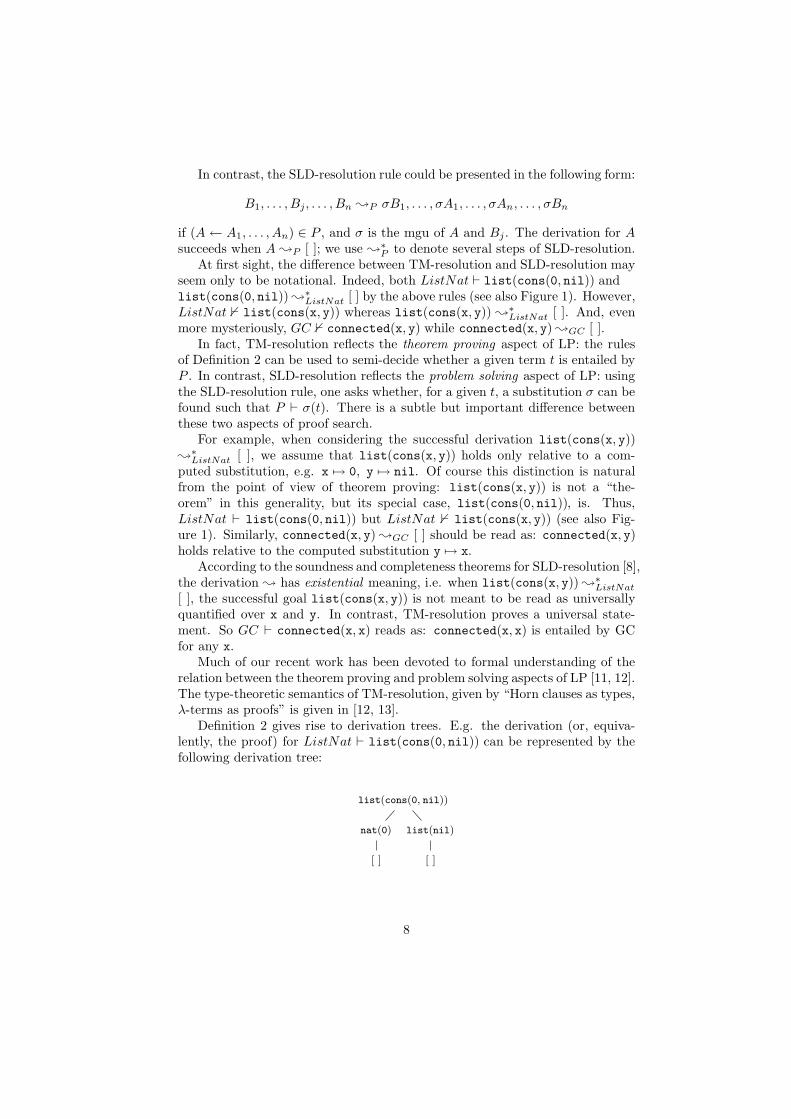
list(cons(0, nil))

nat(0)

[ ]

list(nil)

[ ]

list(nil)

[ ]

list(cons(x, y))

nat(x) list(y)

Figure 1: Left: The coinductive tree for list(cons(0, nil)) and the extended programListNat+. Right: The coinductive tree for list(cons(x, y)) and ListNat+. Each •-nodemarks a clause whose head matches the antecedent of the •-node in the tree.

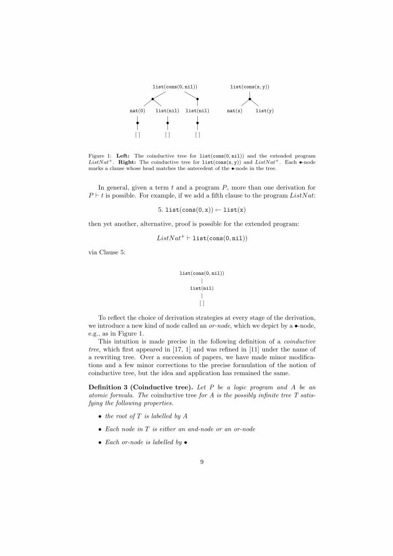
In general, given a term t and a program P , more than one derivation forP ⊢ t is possible. For example, if we add a fifth clause to the program ListNat:

5. list(cons(0, x))← list(x)

then yet another, alternative, proof is possible for the extended program:

ListNat+ ⊢ list(cons(0, nil))

via Clause 5:

list(cons(0, nil))

list(nil)

[ ]

To reflect the choice of derivation strategies at every stage of the derivation,we introduce a new kind of node called an or-node, which we depict by a •-node,e.g., as in Figure 1.

This intuition is made precise in the following definition of a coinductivetree, which first appeared in [17, 1] and was refined in [11] under the name ofa rewriting tree. Over a succession of papers, we have made minor modifica-tions and a few minor corrections to the precise formulation of the notion ofcoinductive tree, but the idea and application has remained the same.

Definition 3 (Coinductive tree). Let P be a logic program and A be anatomic formula. The coinductive tree for A is the possibly infinite tree T satis-fying the following properties.

• the root of T is labelled by A

• Each node in T is either an and-node or an or-node

• Each or-node is labelled by •

9

• Each and-node is labelled by an atom

• For every and-node A′ occurring in T , if there is a clause Ci in P of theform Bi ← Bi

1, . . . , Bini

, such that there is an mgm θ of Bi against A′,then A′ has an or-node as a child, and that or-node has children givenby and-nodes θ(Bi

j), . . . , θ(Bik), where {Bj , . . . , Bk} ⊆ {B1, . . . , Bni

} and

Bj , . . . , Bk is the maximal such set for which θ(Bij), . . . , θ(B

ik) are distinct.

Note the use of mgms (rather than mgus) in the last item. There may existclauses with empty antecedents: some such exist in Figure 1. An or-node, thusa •-node with a single child labelled [ ], represents such a clause.

Coinductive trees provide a convenient model for proofs by TM-resolution.Note that coinductive trees are necessarily finitely branching, logic programsbeing inherently finite.

Let us make one final observation on TM-resolution. Generally, given aprogram P and an atom t, one can prove that

t ❀∗P [ ] with computed substitution σ if and only if P ⊢ σt.

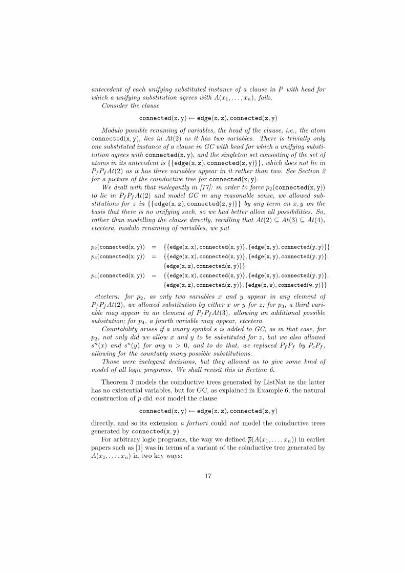
This simple fact may leave the impression that proofs (and correspondinglycoinductive trees) for TM-resolution are in some sense fragments of reductionsby SLD-resolution. Compare, for example, the right-hand tree of Figure 1 be-fore substitution with the larger left-hand tree obtained after the substitution.In this case, we could emulate the problem solving aspect of SLD-resolutionby using coinductive trees and allowing the application of substitutions withincoinductive trees, as was proposed in [28, 11, 12]. That works perfectly forprograms such as ListNat, but not for existential programs: although there is aone step SLD-derivation for connected(x, y) ❀GC [ ] (with y 7→ x), there is noTM-resolution proof for connected(x, y), as the derivation diverges and givesrise to the following infinite coinductive tree:

connected(x, y)

edge(x, z) connected(z, y)

edge(x, w) connected(w, y)

.

..

The above tree is not a fragment of the derivation connected(x, y) ❀GC [ ],moreover, it requires more (infinitely many) variables. Thus, the operationalsemantics of TM-resolution and SLD-resolution can be very different for exis-tential programs, in regard both to termination and to the number of variablesinvolved.

10

This issue is largely orthogonal to that of non-termination. Consider thenon-terminating (but not existential) program Bad:

bad(x)← bad(x)For Bad, the operational behaviours of TM-resolution and SLD-resolution aresimilar: in both cases, derivations do not terminate, and both require onlyfinitely many variables. Moreover, such programs can be analysed using similarcoinductive methods in TM- and SLD-resolution [13, 30].

The problems caused by existential variables are known in the literatureon theorem proving and term-rewriting [29]. In TRS [29], existential variablesare not allowed to appear in rewriting rules, and in type inference based onterm rewriting or TM-resolution, the restriction to non-existential programs iscommon [31].

So theorem-proving, in contrast to problem-solving, is modelled by term-matching; term-matching gives rise to coinductive trees; and as explained in theintroduction and, in more detail, later, coinductive trees give rise to laxness. Soin this paper, we use laxness to model coinductive trees, and thereby theorem-proving in LP, and we relate our semantics with Bonchi and Zanasi’s saturatedsemantics, which we believe primarily models the problem-solving aspect of logicprogramming.

Categorical semantics for existential programs, which are known to be chal-lenging for theorem proving, is a central contribution of Section 6 and of thispaper.

3. Semantics for variable-free logic programs

In this section, we recall and develop the work of [9], in regard to variable-free logic programs, i.e., we take V ar = ∅ in Definition 1. Variable-free logicprograms are operationally equivalent to propositional logic programs, as sub-stitutions play no role in derivations. In this (propositional) setting, coinductivetrees resemble the and-or derivation trees known in the LP literature [4], andthis semantics appears as the ground case of both lax semantics [1] and saturatedsemantics [2].

Proposition 1. For any set At, there is a bijection between the set of variable-free logic programs over the set of atoms At and the set of PfPf -coalgebra struc-tures on At, where Pf is the finite powerset functor on Set.

Theorem 1. Let C(PfPf ) denote the cofree comonad on PfPf . Then, given alogic program P over At, equivalently p : At −→ PfPf (At), the correspondingC(PfPf )-coalgebra p : At −→ C(PfPf )(At) sends an atom A to the coinductivetree for A.

Proof. Applying the work of [32] to this setting, the cofree comonad is ingeneral determined as follows: C(PfPf )(At) is the limit of the diagram

. . . −→ At× PfPf (At× PfPf (At)) −→ At× PfPf (At) −→ At

11

with maps determined by the projection π0 : At × PfPf (At) −→ At, withapplications of the functor At× PfPf (−) to it.

Putting At0 = At and Atn+1 = At× PfPfAtn, and defining the cone

p0 = id : At −→ At(= At0)

pn+1 = 〈id, PfPf (pn) ◦ p〉 : At −→ At× PfPfAtn(= Atn+1)

the limiting property of the diagram determines the coalgebra p : At −→C(PfPf )(At). The image p(A) of an atom A is given by an element of thelimit, equivalently a map from 1 into the limit, equivalently a cone of the dia-gram over 1.

To give the latter is equivalent to giving an element A0 of At, specifi-cally p0(A) = A, together with an element A1 of At × PfPf (At), specificallyp1(A) = (A, p0(A)) = (A, p(A)), together with an element A2 of At×PfPf (At×PfPf (At)), etcetera. The definition of the coinductive tree for A is inherentlycoinductive, matching the definition of the limit, and with the first step agree-ing with the definition of p. Thus it follows by coinduction that p(A) can beidentified with the coinductive tree for A.

Example 3. Let At consist of atoms A, B, C and D. Let P denote the logicprogram

A ← B, C

A ← B, D

D ← A, C

So p(A) = {{B, C}, {B, D}}, p(B) = p(C) = ∅, and p(D) = {{A, C}}.Then, as depicted in Figure 2, p0(A) = A, which is the root of the coinductive

tree for A.Then p1(A) = (A, p(A)) = (A, {{B, C}, {B, D}}), which consists of the same

information as in the first three levels of the coinductive tree for A, i.e., the rootA, two or-nodes, and below each of the two or-nodes, nodes given by each atomin each antecedent of each clause with head A in the logic program P : nodesmarked B and C lie below the first or-node, and nodes marked B and D lie belowthe second or-node, exactly as p1(A) describes.

Continuing, note that p1(D) = (D, p(D)) = (D, {{A, C}}). So

p2(A) = (A, PfPf (p1)(p(A)))= (A, PfPf (p1)({{B, C}, {B, D}}))= (A, {{(B, ∅), (C, ∅)}, {(B, ∅), (D, {{A, C}})}})

which is the same information as that in the first five levels of the coinductivetree for A: p1(A) provides the first three levels of p2(A) because p2(A) must mapto p1(A) in the cone; in the coinductive tree, there are two and-nodes at level 5,labelled by A and C. As there are no clauses with head B or C, no or-nodes lie

12

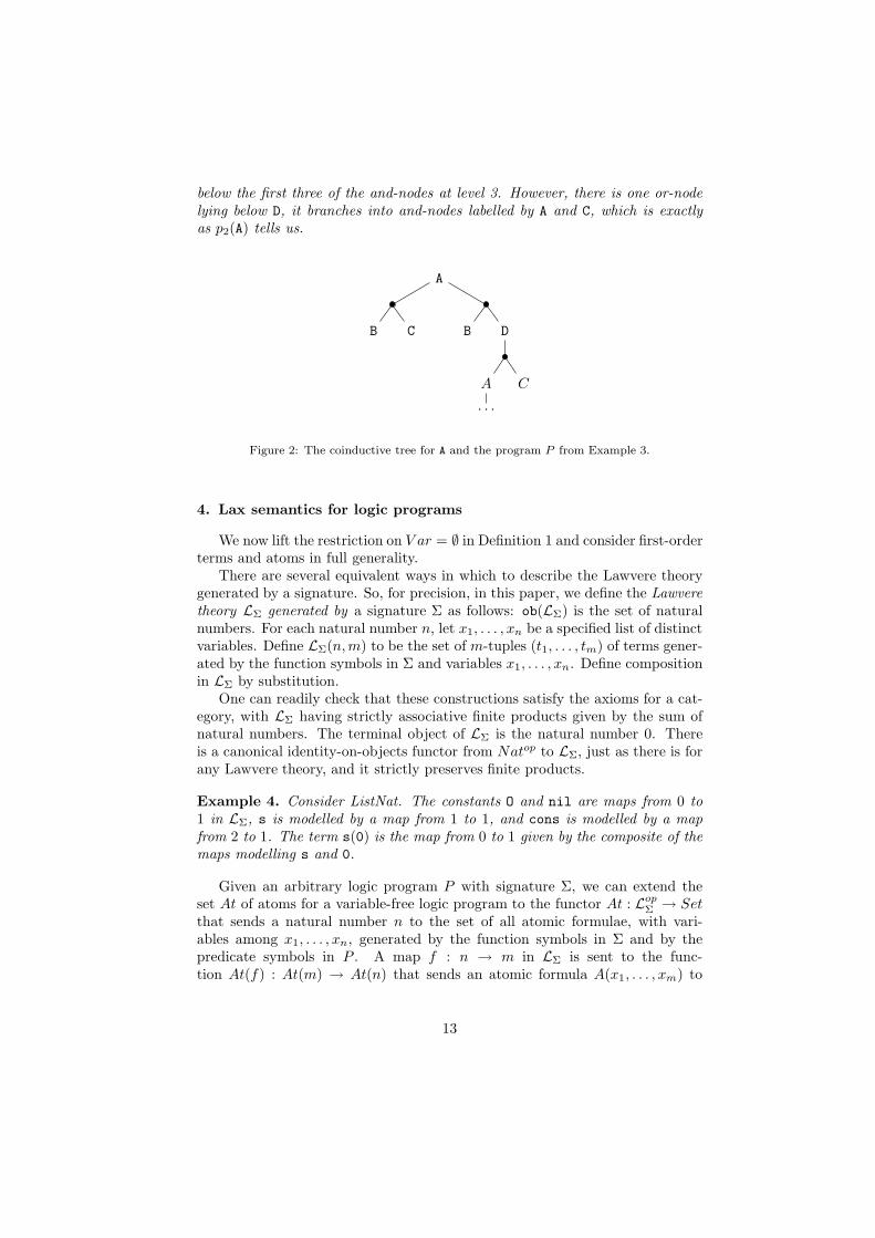
below the first three of the and-nodes at level 3. However, there is one or-nodelying below D, it branches into and-nodes labelled by A and C, which is exactlyas p2(A) tells us.

A

B C B D

A

. . .

C

Figure 2: The coinductive tree for A and the program P from Example 3.

4. Lax semantics for logic programs

We now lift the restriction on V ar = ∅ in Definition 1 and consider first-orderterms and atoms in full generality.

There are several equivalent ways in which to describe the Lawvere theorygenerated by a signature. So, for precision, in this paper, we define the Lawveretheory LΣ generated by a signature Σ as follows: ob(LΣ) is the set of naturalnumbers. For each natural number n, let x1, . . . , xn be a specified list of distinctvariables. Define LΣ(n, m) to be the set of m-tuples (t1, . . . , tm) of terms gener-ated by the function symbols in Σ and variables x1, . . . , xn. Define compositionin LΣ by substitution.

One can readily check that these constructions satisfy the axioms for a cat-egory, with LΣ having strictly associative finite products given by the sum ofnatural numbers. The terminal object of LΣ is the natural number 0. Thereis a canonical identity-on-objects functor from Natop to LΣ, just as there is forany Lawvere theory, and it strictly preserves finite products.

Example 4. Consider ListNat. The constants O and nil are maps from 0 to1 in LΣ, s is modelled by a map from 1 to 1, and cons is modelled by a mapfrom 2 to 1. The term s(0) is the map from 0 to 1 given by the composite of themaps modelling s and 0.

Given an arbitrary logic program P with signature Σ, we can extend theset At of atoms for a variable-free logic program to the functor At : Lop

Σ → Setthat sends a natural number n to the set of all atomic formulae, with vari-ables among x1, . . . , xn, generated by the function symbols in Σ and by thepredicate symbols in P . A map f : n → m in LΣ is sent to the func-tion At(f) : At(m) → At(n) that sends an atomic formula A(x1, . . . , xm) to

13

A(f1(x1, . . . , xn)/x1, . . . , fm(x1, . . . , xn)/xm), i.e., At(f) is defined by substitu-tion.

As explained in the Introduction and in [9], we cannot model a logic programby a natural transformation of the form p : At −→ PfPfAt as naturality breaksdown, e.g., in ListNat. So, in [17, 1], we relaxed naturality to lax naturality.In order to define it, we extended At : Lop

Σ → Set to have codomain Poset bycomposing At with the inclusion of Set into Poset. Mildly overloading notation,we denote the composite by At : Lop

Σ → Poset.

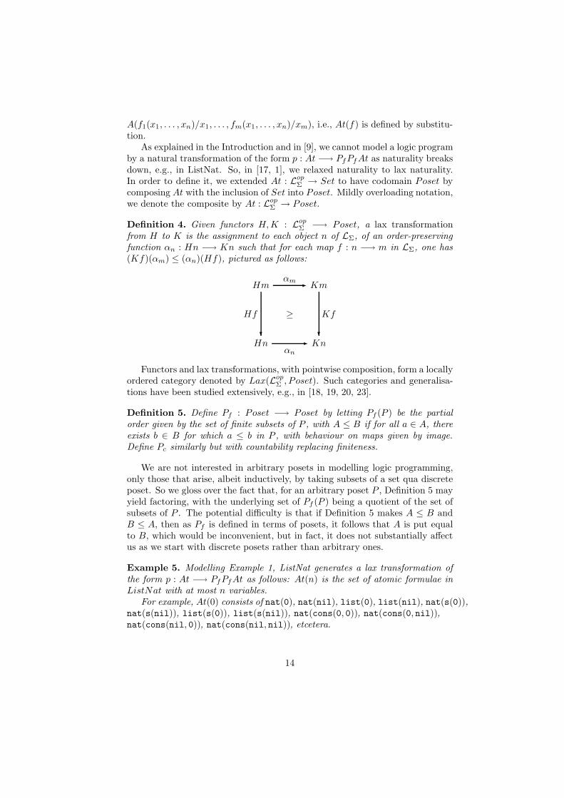
Definition 4. Given functors H, K : LopΣ −→ Poset, a lax transformation

from H to K is the assignment to each object n of LΣ, of an order-preservingfunction αn : Hn −→ Kn such that for each map f : n −→ m in LΣ, one has(Kf)(αm) ≤ (αn)(Hf), pictured as follows:

Hmαm

✲ Km

≥

Hn

Hf

❄

αn

✲ Kn

Kf

❄

Functors and lax transformations, with pointwise composition, form a locallyordered category denoted by Lax(Lop

Σ , Poset). Such categories and generalisa-tions have been studied extensively, e.g., in [18, 19, 20, 23].

Definition 5. Define Pf : Poset −→ Poset by letting Pf (P ) be the partialorder given by the set of finite subsets of P , with A ≤ B if for all a ∈ A, thereexists b ∈ B for which a ≤ b in P , with behaviour on maps given by image.Define Pc similarly but with countability replacing finiteness.

We are not interested in arbitrary posets in modelling logic programming,only those that arise, albeit inductively, by taking subsets of a set qua discreteposet. So we gloss over the fact that, for an arbitrary poset P , Definition 5 mayyield factoring, with the underlying set of Pf (P ) being a quotient of the set ofsubsets of P . The potential difficulty is that if Definition 5 makes A ≤ B andB ≤ A, then as Pf is defined in terms of posets, it follows that A is put equalto B, which would be inconvenient, but in fact, it does not substantially affectus as we start with discrete posets rather than arbitrary ones.

Example 5. Modelling Example 1, ListNat generates a lax transformation ofthe form p : At −→ PfPfAt as follows: At(n) is the set of atomic formulae inListNat with at most n variables.

For example, At(0) consists of nat(0), nat(nil), list(0), list(nil), nat(s(0)),nat(s(nil)), list(s(0)), list(s(nil)), nat(cons(0, 0)), nat(cons(0, nil)),nat(cons(nil, 0)), nat(cons(nil, nil)), etcetera.

14

Similarly, At(1) includes all atomic formulae containing at most one (spec-ified) variable x, thus all the elements of At(0) together with nat(x), list(x),nat(s(x)), list(s(x)), nat(cons(0, x)), nat(cons(x, 0)), nat(cons(x, x)), etcetera.

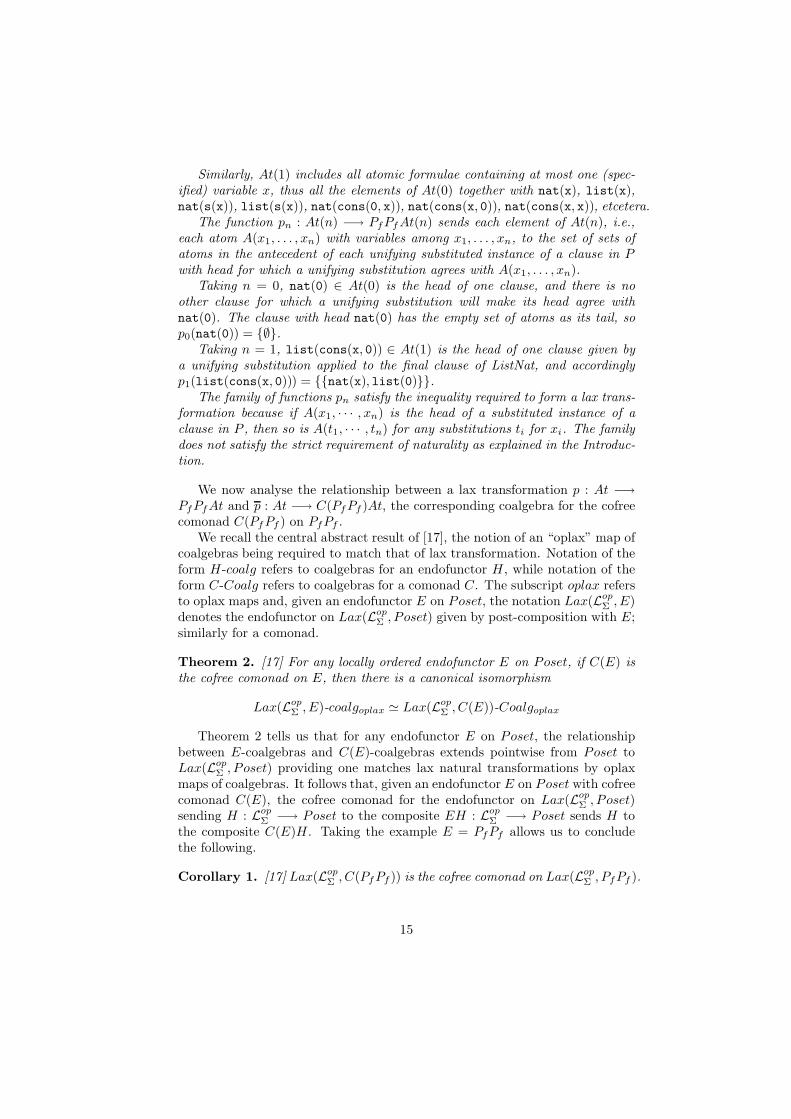
The function pn : At(n) −→ PfPfAt(n) sends each element of At(n), i.e.,each atom A(x1, . . . , xn) with variables among x1, . . . , xn, to the set of sets ofatoms in the antecedent of each unifying substituted instance of a clause in Pwith head for which a unifying substitution agrees with A(x1, . . . , xn).

Taking n = 0, nat(0) ∈ At(0) is the head of one clause, and there is noother clause for which a unifying substitution will make its head agree withnat(0). The clause with head nat(0) has the empty set of atoms as its tail, sop0(nat(0)) = {∅}.

Taking n = 1, list(cons(x, 0)) ∈ At(1) is the head of one clause given bya unifying substitution applied to the final clause of ListNat, and accordinglyp1(list(cons(x, 0))) = {{nat(x), list(0)}}.

The family of functions pn satisfy the inequality required to form a lax trans-formation because if A(x1, · · · , xn) is the head of a substituted instance of aclause in P , then so is A(t1, · · · , tn) for any substitutions ti for xi. The familydoes not satisfy the strict requirement of naturality as explained in the Introduc-tion.

We now analyse the relationship between a lax transformation p : At −→PfPfAt and p : At −→ C(PfPf )At, the corresponding coalgebra for the cofreecomonad C(PfPf ) on PfPf .

We recall the central abstract result of [17], the notion of an “oplax” map ofcoalgebras being required to match that of lax transformation. Notation of theform H-coalg refers to coalgebras for an endofunctor H , while notation of theform C-Coalg refers to coalgebras for a comonad C. The subscript oplax refersto oplax maps and, given an endofunctor E on Poset, the notation Lax(Lop

Σ , E)denotes the endofunctor on Lax(Lop

Σ , Poset) given by post-composition with E;similarly for a comonad.

Theorem 2. [17] For any locally ordered endofunctor E on Poset, if C(E) isthe cofree comonad on E, then there is a canonical isomorphism

Lax(LopΣ , E)-coalgoplax ≃ Lax(Lop

Σ , C(E))-Coalgoplax

Theorem 2 tells us that for any endofunctor E on Poset, the relationshipbetween E-coalgebras and C(E)-coalgebras extends pointwise from Poset toLax(Lop

Σ , Poset) providing one matches lax natural transformations by oplaxmaps of coalgebras. It follows that, given an endofunctor E on Poset with cofreecomonad C(E), the cofree comonad for the endofunctor on Lax(Lop

Σ , Poset)sending H : Lop

Σ −→ Poset to the composite EH : LopΣ −→ Poset sends H to

the composite C(E)H . Taking the example E = PfPf allows us to concludethe following.

Corollary 1. [17] Lax(LopΣ , C(PfPf )) is the cofree comonad on Lax(Lop

Σ , PfPf ).

15

Corollary 1 means that there is a natural bijection between lax transformations

p : At −→ PfPfAt

and lax transformations

p : At −→ C(PfPf )At

subject to the two conditions required of a coalgebra of a comonad given point-wise, thus by applying the construction of Theorem 1 pointwise. So it is theabstract result we need in order to characterise the coinductive trees gener-ated by logic programs with no existential variables, extending Theorem 1. Asexplained in the Introduction, an existential variable in a logic program is avariable that appears in the tail of a clause but not in its head. We explain thesituation in detail in Example 6, but for now, just note that ListNat does nothave existential variables, so the following result applies directly to it.

Theorem 3. Let C(PfPf ) denote the cofree comonad on the endofunctor PfPf

on Poset. Then, given a logic program P with no existential variables on At,defining pn(A(x1, . . . , xn)) to be the set of sets of atoms in each antecedent ofeach unifying substituted instance of a clause in P with head for which a unifyingsubstitution agrees with A(x1, . . . , xn), the corresponding Lax(Lop

Σ , C(PfPf ))-coalgebra p : At −→ C(PfPf )At sends an atom A(x1, . . . , xn) to the coinductivetree for A(x1, . . . , xn).

Proof. The absence of existential variables ensures that any variable that ap-pears in the antecedent of a clause must also appear in its head. So every atomin every antecedent of every unifying substituted instance of a clause in P withhead for which a unifying substitution agrees with A(x1, . . . , xn) actually lies inAt(n). Moreover, there are only finitely many sets of sets of such atoms. So theconstruction of each pn is well-defined, i.e., the image of A(x1, . . . , xn) lies inPfPfAt(n). The collection of maps given by pn for each object n of LΣ formsa lax transformation from At to PfPfAt: the laxness condition holds becausesubstitution preserves the truth of a clause, i.e., if one makes a substitution intoboth the head and tail of a clause that is true, the substituted instance of theclause is also true.

By Corollary 1, p is determined pointwise. So, to construct it, we may fixn and follow the proof of Theorem 1, consistently replacing At by At(n). Tocomplete the proof, observe that the construction of p from a logic program Pmatches the construction of the coinductive tree for an atom A(x1, . . . , xn) if Phas no existential variables. So following the proof of Theorem 1 completes thisproof.

Example 6. Attempting to model Example 2, that of graph connectedness, GC,by mimicking the modelling of ListNat in Example 5, i.e., defining the functionpn : At(n) −→ PfPfAt(n) by sending each element of At(n), i.e., each atomA(x1, . . . , xn) with variables among x1, . . . , xn, to the set of sets of atoms in the

16

antecedent of each unifying substituted instance of a clause in P with head forwhich a unifying substitution agrees with A(x1, . . . , xn), fails.

Consider the clause

connected(x, y)← edge(x, z), connected(z, y)

Modulo possible renaming of variables, the head of the clause, i.e., the atomconnected(x, y), lies in At(2) as it has two variables. There is trivially onlyone substituted instance of a clause in GC with head for which a unifying substi-tution agrees with connected(x, y), and the singleton set consisting of the set ofatoms in its antecedent is {{edge(x, z), connected(z, y)}}, which does not lie inPfPfAt(2) as it has three variables appear in it rather than two. See Section 2for a picture of the coinductive tree for connected(x, y).

We dealt with that inelegantly in [17]: in order to force p2(connected(x, y))to lie in PfPfAt(2) and model GC in any reasonable sense, we allowed sub-stitutions for z in {{edge(x, z), connected(z, y)}} by any term on x, y on thebasis that there is no unifying such, so we had better allow all possibilities. So,rather than modelling the clause directly, recalling that At(2) ⊆ At(3) ⊆ At(4),etcetera, modulo renaming of variables, we put

p2(connected(x, y)) = {{edge(x, x), connected(x, y)}, {edge(x, y), connected(y, y)}}

p3(connected(x, y)) = {{edge(x, x), connected(x, y)}, {edge(x, y), connected(y, y)},

{edge(x, z), connected(z, y)}}

p4(connected(x, y)) = {{edge(x, x), connected(x, y)}, {edge(x, y), connected(y, y)},

{edge(x, z), connected(z, y)}, {edge(x, w), connected(w, y)}}

etcetera: for p2, as only two variables x and y appear in any element ofPfPfAt(2), we allowed substitution by either x or y for z; for p3, a third vari-able may appear in an element of PfPfAt(3), allowing an additional possiblesubsitution; for p4, a fourth variable may appear, etcetera.

Countability arises if a unary symbol s is added to GC, as in that case, forp2, not only did we allow x and y to be substituted for z, but we also allowedsn(x) and sn(y) for any n > 0, and to do that, we replaced PfPf by PcPf ,allowing for the countably many possible substitutions.

Those were inelegant decisions, but they allowed us to give some kind ofmodel of all logic programs. We shall revisit this in Section 6.

Theorem 3 models the coinductive trees generated by ListNat as the latterhas no existential variables, but for GC, as explained in Example 6, the naturalconstruction of p did not model the clause

connected(x, y)← edge(x, z), connected(z, y)

directly, and so its extension a fortiori could not model the coinductive treesgenerated by connected(x, y).

For arbitrary logic programs, the way we defined p(A(x1, . . . , xn)) in earlierpapers such as [1] was in terms of a variant of the coinductive tree generated byA(x1, . . . , xn) in two key ways:

17

1. coinductive trees allow new variables to be introduced as one passes downthe tree, e.g., with

connected(x, y)← edge(x, z), connected(z, y)

appearing in it. However, because of the presence of the variable z, theset {{edge(x, z), connected(z, y)}} does not appear in PfPfAt(2). Inprevious papers, we made clumsy adaptations of the natural model inorder to model the clause.

2. coinductive trees are finitely branching, as one expects in logic program-ming, but in previous papers, we allowed p(A(x1, . . . , xn)) to be infinitelybranching in order to model the countably many possible applications ofa unary function symbol.

5. Saturated semantics for logic programs

Bonchi and Zanasi’s saturated semantics approach to modelling logic pro-gramming in [14] was to consider PfPf as we did in [17], sending At to PfPfAt,but to ignore the inherent laxness, replacing Lax(Lop

Σ , Poset) by [ob(LΣ), Set],where ob(LΣ) is the set of objects of LΣ treated as a discrete category, i.e., as acategory containing only identity maps. Their central construction may be seenin a more axiomatic setting as follows.

For any small category C, let ob(C) denote the discrete subcategory withthe same objects as C, with inclusion I : ob(C) −→ C. Then the functor

[I, Set] : [C, Set] −→ [ob(C), Set]

has a right adjoint given by right Kan extension, and that remains true whenone extends from Set to any complete category, and it all enriches, e.g., overPoset [3]. As ob(C) has no non-trivial arrows, the right Kan extension is aproduct, given by

(ranIH)(c) =∏d∈C

HdC(c,d)

By the Yoneda lemma, to give a natural transformation from K to (ranIH)(−)is equivalent to giving a natural, or equivalently in this setting, a “not necessarilynatural”, transformation from KI to H . Taking C = Lop

Σ gives exactly Bonchiand Zanasi’s formulation of saturated semantics [14].

It was the fact of the existence of the right adjoint, rather than its characteri-sation as a right Kan extension, that enabled Bonchi and Zanasi’s constructionsof saturation and desaturation, but the description as a right Kan extensioninformed their syntactic analysis.

Note for later that products in Poset are given pointwise, so agree withproducts in Set. So if we replace Set by Poset here, and if C is an ordinarycategory without any non-trivial Poset-enrichment, the right Kan extension

18

would yield the same set as above, with an order on it determined by that onH .

In order to unify saturated semantics with lax semantics, we need to rephraseBonchi and Zanasi’s formulation a little. Upon close inspection, one can seethat, in their semantics, they only used objects of [ob(LΣ)op, Set], equivalently[ob(LΣ), Set], of the form HI for some H : Lop

Σ −→ Set [14]. That allows us,while making no substantive change to their body of work, to reformulate it alittle, in axiomatic terms, as follows.

Let [C, Set]d denote the category of functors from C to Set and “not neces-sarily natural” transformations between them, i.e., a map from H to K consistsof, for all c ∈ C, a function αc : Hc −→ Kc, without demanding a naturalitycondition. The functor [I, Set] : [C, Set] −→ [ob(C), Set] factors through theinclusion of [C, Set] into [C, Set]d as follows:

[C, Set]JSet

✲ [C, Set]dJ ′

✲ [ob(C), Set]

The functor J ′ : [C, Set]d −→ [ob(C), Set] sends a functor H : C −→ Set to thefunctor HI : ob(C) −→ Set. The composite [I, Set] = J ′JSet has a right adjointgiven by right Kan extension, and J ′ is fully faithful. By elementary categorytheory [33], it follows that JSet : [C, Set] −→ [C, Set]d has a right adjoint thatsends H : C −→ Set to the right Kan extension of J ′(H) = HI along I.

Thus one can rephrase Bonchi and Zanasi’s work to assert that the centralmathematical fact that supports saturated semantics is that the inclusion

[LopΣ , Set] −→ [Lop

Σ , Set]d

has a right adjoint that sends a functor H : LopΣ −→ Set to the right Kan

extension ranIHI of the composite HI : ob(LΣ)op −→ Set along the inclusionI : ob(LΣ) −→ LΣ.

We can now unify lax semantics with saturated semantics by developing aprecise body of theory that relates the inclusion

JSet : [C, Set] −→ [C, Set]d

which has a right adjoint that sends H : C −→ Set to ranIHI, with theinclusion

J : [C, Poset] −→ Lax(C, Poset)

which also has a right adjoint, that right adjoint being given by a restriction ofthe right Kan extension ranIHI of the composite HI : ob(C) −→ Poset alongthe inclusion I : ob(C) −→ C.

The existence of the right adjoint follows from Theorem 3.13 of [19], but wegive an independent proof here and a description of it in terms of right Kanextensions in order to show that Bonchi and Zanasi’s explicit constructions ofsaturation and desaturation apply equally in this setting.

Consider the inclusions

[C, Poset] −→ Lax(C, Poset) −→ [C, Poset]d

19

Exactly as for Set as above, for any small category C, the inclusion

JPoset : [C, Poset] −→ [C, Poset]d

has a right adjoint sending H : C −→ Poset to ranIHI. In order to give aright adjoint to J : [C, Poset] −→ Lax(C, Poset), we will restrict ranIHI to asubfunctor R(H) in [C, Poset] so that to give a natural transformation from Kinto the restriction R(H) of ranIHI is equivalent to giving a map from K to Hin Lax(C, Poset), i.e., a map in [C, Poset]d that satisfies the condition that, forall f : c −→ d, one has Hf.αc ≤ αd.Kf . This can be done by defining R(H) tobe an inserter, which is a particularly useful kind of limit that applies to locallyordered categories and is a particular kind of generalisation of the notion ofequaliser.

Definition 6. [19] Given parallel maps f, g : X −→ Y in a locally orderedcategory D, an inserter from f to g is an object Ins(f, g) of D together witha map i : Ins(f, g) −→ X such that fi ≤ gi and is universal such, i.e., forany object Z and map z : Z −→ X for which fz ≤ gz, there is a unique mapk : Z −→ Ins(f, g) such that ik = z. Moreover, for any such z and z′ for whichz ≤ z′, then k ≤ k′, where k and k′ are induced by z and z′ respectively.

An inserter is a form of limit. Taking D to be Poset, the poset Ins(f, g) isgiven by the full sub-poset of X determined by {x ∈ X |f(x) ≤ g(x)}. Beinglimits, inserters in functor categories are determined pointwise.

The inserter we require is subtle, in the spirit of the work of [19] and [3].Given a functor H : C −→ Poset, we define a parallel pair of maps in [C, Poset],i.e., natural transformations, δ1 and δ2. Their domains and codomains, whichmust be functors from C to Poset, are given as follows:

δ1, δ2 :∏d∈C

HdC(−,d) −→∏

d,d′∈C

Hd′C(−,d)×C(d,d′)

i.e., the domain of both δ1 and δ2 is the functor from C to Poset that sends cto

∏d∈C HdC(c,d), and similarly for the codomain.

Using the property of products, to give such natural transformations is equiv-alent, via Currying, to giving, for each c, d and d′ in C, maps of the form

(δ1)(d,d′)c, (δ2)(d,d′)c : C(c, d) × C(d, d′)×∏d∈C

HdC(c,d) −→ Hd′

natural in c. We define the two maps as follows:

1. the (d, d′)-component of δ1c is determined by composing

◦C × id : C(c, d) × C(d, d′)×∏d∈C

HdC(c,d) −→ C(c, d′)×∏d∈C

HdC(c,d)

with the evaluation of the product at d′, i.e., taking the d′-th componentof the product and applying evaluation to C(c, d′)×HdC(c,d′)

20

2. the (d, d′)-component of δ2c is determined by evaluating the product at d

C(c, d)× C(d, d′)×∏d∈C

HdC(c,d) −→ C(d, d′)×Hd

then composing with

C(d, d′)×HdH × id

✲ Hd′Hd ×Hdeval

✲ Hd′

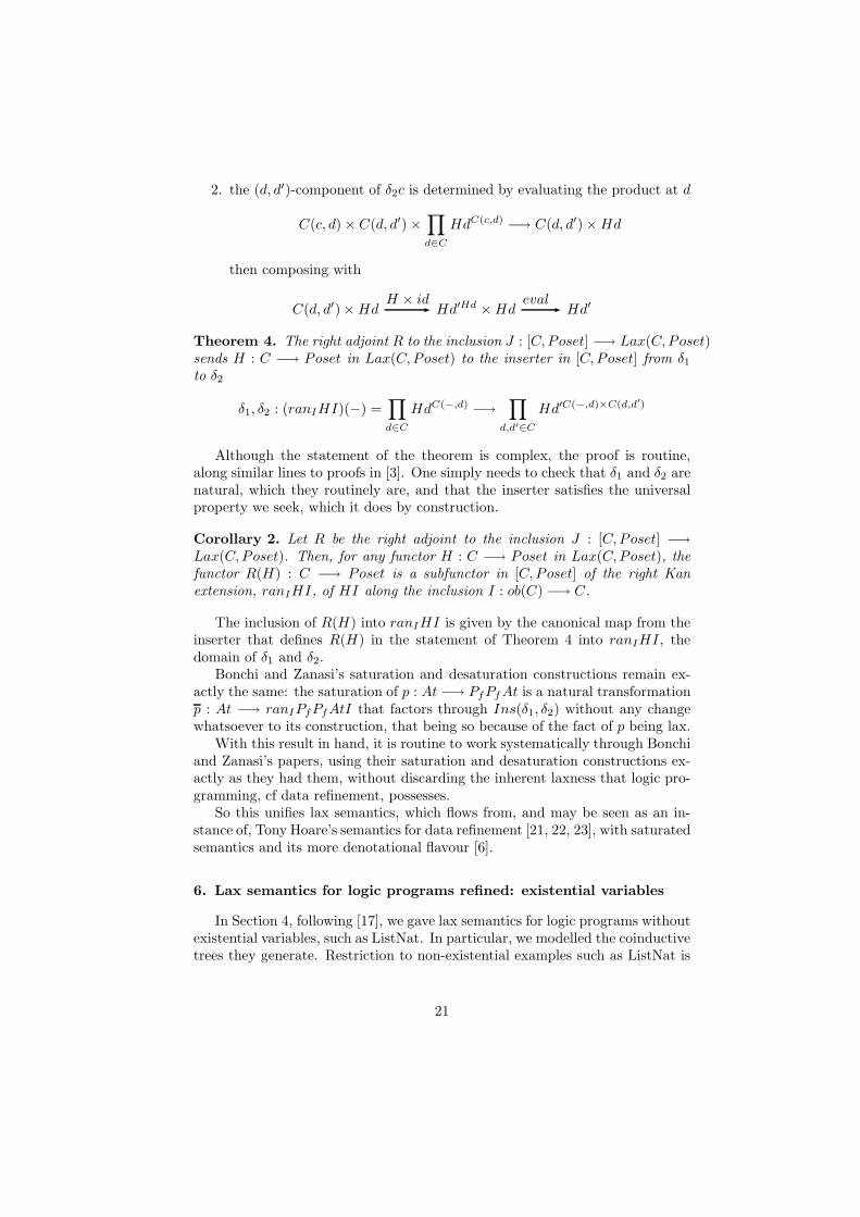
Theorem 4. The right adjoint R to the inclusion J : [C, Poset] −→ Lax(C, Poset)sends H : C −→ Poset in Lax(C, Poset) to the inserter in [C, Poset] from δ1

to δ2

δ1, δ2 : (ranIHI)(−) =∏d∈C

HdC(−,d) −→∏

d,d′∈C

Hd′C(−,d)×C(d,d′)

Although the statement of the theorem is complex, the proof is routine,along similar lines to proofs in [3]. One simply needs to check that δ1 and δ2 arenatural, which they routinely are, and that the inserter satisfies the universalproperty we seek, which it does by construction.

Corollary 2. Let R be the right adjoint to the inclusion J : [C, Poset] −→Lax(C, Poset). Then, for any functor H : C −→ Poset in Lax(C, Poset), thefunctor R(H) : C −→ Poset is a subfunctor in [C, Poset] of the right Kanextension, ranIHI, of HI along the inclusion I : ob(C) −→ C.

The inclusion of R(H) into ranIHI is given by the canonical map from theinserter that defines R(H) in the statement of Theorem 4 into ranIHI, thedomain of δ1 and δ2.

Bonchi and Zanasi’s saturation and desaturation constructions remain ex-actly the same: the saturation of p : At −→ PfPfAt is a natural transformationp : At −→ ranIPfPfAtI that factors through Ins(δ1, δ2) without any changewhatsoever to its construction, that being so because of the fact of p being lax.

With this result in hand, it is routine to work systematically through Bonchiand Zanasi’s papers, using their saturation and desaturation constructions ex-actly as they had them, without discarding the inherent laxness that logic pro-gramming, cf data refinement, possesses.

So this unifies lax semantics, which flows from, and may be seen as an in-stance of, Tony Hoare’s semantics for data refinement [21, 22, 23], with saturatedsemantics and its more denotational flavour [6].

6. Lax semantics for logic programs refined: existential variables

In Section 4, following [17], we gave lax semantics for logic programs withoutexistential variables, such as ListNat. In particular, we modelled the coinductivetrees they generate. Restriction to non-existential examples such as ListNat is

21

common for implementational reasons [1, 11, 12, 13], so Section 4 allowed themodelling of coinductive trees for a natural class of logic programs.

Nevertheless, we would like to model coinductive trees generated by logicprogramming in full generality, including examples such as that of GC. Weneed to refine the lax semantics of Section 4 in order to do so, and, having justunified lax semantics with saturated semantics in Section 5, we would like toretain that unity in making such a refinement. So that is what we do in thissection.

We initially proposed such a refinement in the workshop paper [25] thatthis paper extends, but since the workshop, we have found a further refinementthat strengthens the relationship with the modelling of local state [26]. So ourconstructions here are a little different to those in [25].

In order to model coinductive trees, it follows from Example 6 that theendofunctor Lax(Lop

Σ , PfPf ) on Lax(LopΣ , Poset) that sends At to PfPfAt, needs

to be refined as {{edge(x, z), connected(z, y)}} is not an element of PfPfAt(2)as it involves three variables x, y and z. In general, we need to allow the im-age of pn to lie in the set given by applying PfPf to a superset of At(n), onethat includes At(m) for all m ≥ n. In Example 6, that would allow the imageof p2 to lie in PfPfAt(3) rather than in PfPfAt(2), thus allowing us to mapconnected(x, y) to {{edge(x, z), connected(z, y)}} as desired.

However, we do not want to double-count: there are six injections of 2 into3, inducing six inclusions At(2) ⊆ At(3), and one only wants to count each atomin At(2) once. So we refine PfPfAt(n) to become PfPf (

∫At(n)), where

∫At is

defined as follows.Letting Inj denote the category of natural numbers and injections, for any

Lawvere theory L, there is a canonical identity-on-objects functor J : Injop −→L.

Definition 7. We define∫At(n) to be the colimit of the composite functor

n/Injcod

✲ InjJ

✲ LopΣ

At✲ Poset

This functor sends an injection j : n −→ m to At(m), with the j-th compo-nent of the colimiting cocone being of the form ρj : At(m) −→

∫At(n).

The colimiting property is precisely the condition required to ensure nodouble-counting (see [33] or, for the enriched version, [3] of this construction ina general setting).

It is not routine to extend the construction of∫At(n) for each n to give a

functor∫At : Lop

Σ −→ Poset. To do so, we mimic the construction on arrowsused to define the monad for local state in [26]. We first used this idea in [25]and we refine our use of it in this paper to make for a closer technical relation-ship with the semantics of local state in [26]: we do not fully understand therelationship yet, but there seems considerable potential based on the work hereto make precise comparison between the role of variables in logic programmingwith that of worlds in modelling local state.

22

Following [26], we extend∫

At(n) to a functor∫At : Lop

Σ −→ Poset by send-ing a map f : n −→ n′ in LΣ to the order-preserving function

∫At(f) :

∫At(n′) −→

∫At(n)

determined by the colimiting property of∫

At(n′) as follows.For each j′ : n′ −→ l ∈ n′/Inj, there are a unique natural number k and at

least one isomorphism between l and n′ + k, such that composite of j′ with theisomorphism is the canonical injection from n′ to n′ +k. So, in calculating withthe colimit, we may identify j′, via composition with a chosen such isomorphism,with the canonical injection from n′ to n′ + k. This induces a cocone

At(l) ∼= At(n′ + k)At(f + k)

✲ At(n + k)ρj✲

∫At(n)

where j : n −→ n+k is the canonical injection of n into n+k, thus determining∫At(f). It is routine to check that this assignment makes

∫At functorial with

respect to maps in LopΣ .

There is nothing specific about the functor At : LopΣ −→ Poset in the above

construction. The construction generalises without fuss from defining the func-tor

∫At : Lop

Σ −→ Poset to the definition of∫H : Lop

Σ −→ Poset for any functorH : Lop

Σ −→ Poset.In order to make each map α : H ⇒ K generate a map

∫α :

∫H ⇒

∫K, we

need to specify in exactly what category we treat H as an object. Lax(LopΣ , Poset)

is not possible because∫H(n) is defined to be a (strict rather than lax) col-

imit, so a (strict) cocone into∫K(n) is required in order to generate the map∫

α(n) :∫

H(n) →∫

K(n). We would have that if we had strict naturalityof α with respect to injections, but that is not true of an arbitrary map α inLax(Lop

Σ , Poset). So we refine Lax(LopΣ , Poset) by restricting its maps in order

to do that.We accordingly restrict the maps of Lax(Lop

Σ , Poset) to allow only those laxtransformations α : H ⇒ K that are strict with respect to maps in Inj, i.e.,those α such that for any injection i : n −→ m, the diagram

Hnαn

✲ Kn

Hm

Hi

❄

αm

✲ Km

Ki

❄

commutes. A restriction of this nature is standard in 2-category theory, e.g.,in [19], as one typically needs to distinguish between lax and strict maps, withstrict commutativity only in regard to the latter.

Summarising this discussion yields the following:

23

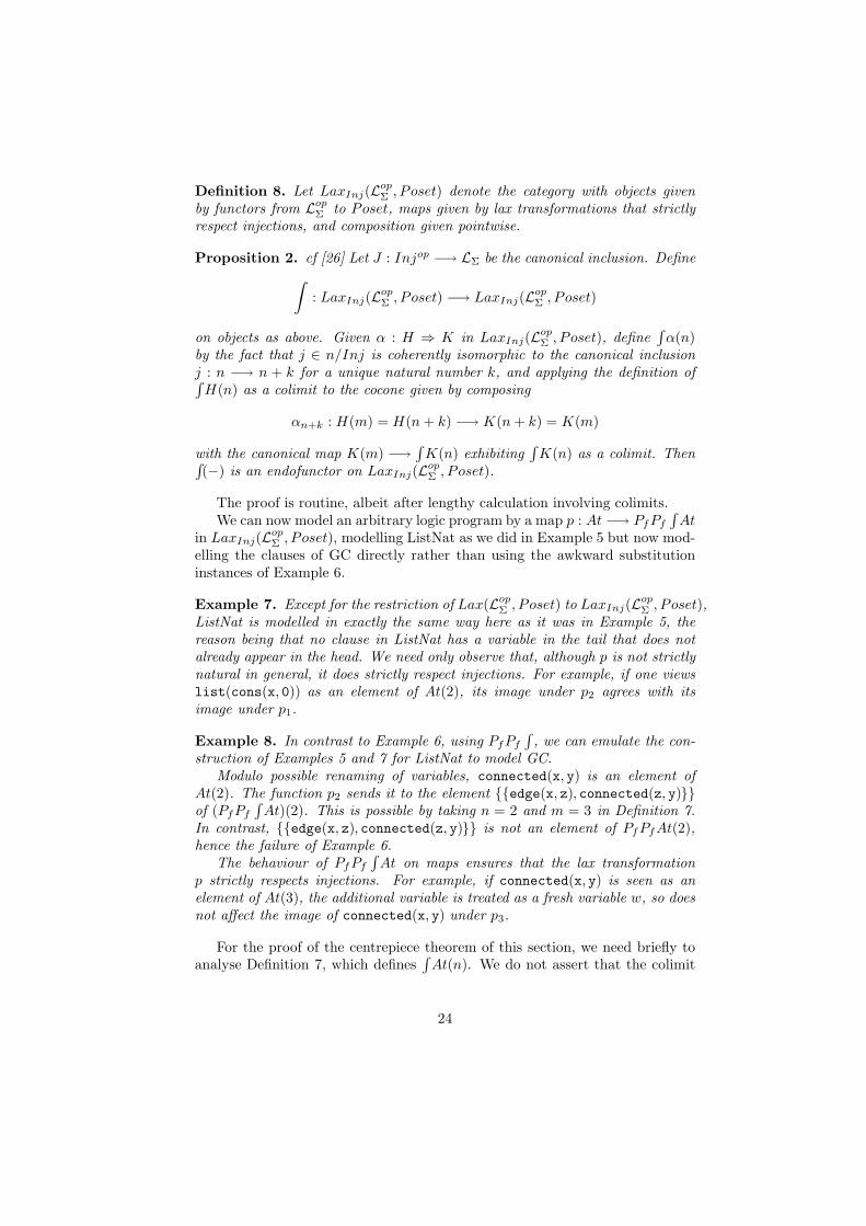
Definition 8. Let LaxInj(LopΣ , Poset) denote the category with objects given

by functors from LopΣ to Poset, maps given by lax transformations that strictly

respect injections, and composition given pointwise.

Proposition 2. cf [26] Let J : Injop −→ LΣ be the canonical inclusion. Define

∫: LaxInj(L

opΣ , Poset) −→ LaxInj(L

opΣ , Poset)

on objects as above. Given α : H ⇒ K in LaxInj(LopΣ , Poset), define

∫α(n)

by the fact that j ∈ n/Inj is coherently isomorphic to the canonical inclusionj : n −→ n + k for a unique natural number k, and applying the definition of∫H(n) as a colimit to the cocone given by composing

αn+k : H(m) = H(n + k) −→ K(n + k) = K(m)

with the canonical map K(m) −→∫

K(n) exhibiting∫K(n) as a colimit. Then∫

(−) is an endofunctor on LaxInj(LopΣ , Poset).

The proof is routine, albeit after lengthy calculation involving colimits.We can now model an arbitrary logic program by a map p : At −→ PfPf

∫At

in LaxInj(LopΣ , Poset), modelling ListNat as we did in Example 5 but now mod-

elling the clauses of GC directly rather than using the awkward substitutioninstances of Example 6.

Example 7. Except for the restriction of Lax(LopΣ , Poset) to LaxInj(L

opΣ , Poset),

ListNat is modelled in exactly the same way here as it was in Example 5, thereason being that no clause in ListNat has a variable in the tail that does notalready appear in the head. We need only observe that, although p is not strictlynatural in general, it does strictly respect injections. For example, if one viewslist(cons(x, 0)) as an element of At(2), its image under p2 agrees with itsimage under p1.

Example 8. In contrast to Example 6, using PfPf

∫, we can emulate the con-

struction of Examples 5 and 7 for ListNat to model GC.Modulo possible renaming of variables, connected(x, y) is an element of

At(2). The function p2 sends it to the element {{edge(x, z), connected(z, y)}}of (PfPf

∫At)(2). This is possible by taking n = 2 and m = 3 in Definition 7.

In contrast, {{edge(x, z), connected(z, y)}} is not an element of PfPfAt(2),hence the failure of Example 6.

The behaviour of PfPf

∫At on maps ensures that the lax transformation

p strictly respects injections. For example, if connected(x, y) is seen as anelement of At(3), the additional variable is treated as a fresh variable w, so doesnot affect the image of connected(x, y) under p3.

For the proof of the centrepiece theorem of this section, we need briefly toanalyse Definition 7, which defines

∫At(n). We do not assert that the colimit

24

defining∫At(n) is ω-directed, but it can be built from an ω-directed colimit as

follows.For any injection j : n −→ l, there are a unique k and at least one isomor-

phism between l and n+k such that the composite of j with the isomorphism isthe canonical injection from n to n + k. There may be more than one such iso-morphism: for instance, if n = 2 and l = 4, there are two. So the colimit

∫At(n)

is given by first taking the ω-directed colimit colimm≥nAt(m) determined bythe canonical injections, then by quotienting colimm≥nAt(m) by structural per-mutations. This extends routinely to arbitrary functors.

Lemma 1. The construction∫

preserves monomorphisms in [Inj, Poset].

Proof. Monomorphisms in [Inj, Poset] are given pointwise. An ω-directedcolimit is, a fortiori, a filtered colimit, so, by Gabriel-Ulmer, it commutes withfinite limits, so respects monomorphisms. So, given a monomorphism ι : H ⇒K, for any n, the induced map from colimm≥nH(m) to colimm≥nK(m) is amonomorphism.

∫H(n) is the quotient of colimm≥nH(m) under structural

permutations; likewise for∫K(n). Given two elements of colimm≥nH(m) that

are sent by ι to equivalent elements of colimm≥nK(m), without loss of generality,a permutation θ in Inj generates the equivalence. Naturality of ι, together withinjectivity of ιm, implies that applying H(θ) to the original two elements ofcolimm≥nH(m) also renders them equivalent, thus yielding injectivity of

∫ι(n).

Theorem 5. The functor PfPf

∫: LaxInj(L

opΣ , Poset) −→ LaxInj(L

opΣ , Poset)

induces a cofree comonad C(PfPf

∫) on LaxInj(L

opΣ , Poset). Moreover, given

a logic program P qua PfPf

∫-coalgebra p : At −→ PfPf

∫At, the corresponding

C(PfPf

∫)-coalgebra p : At −→ C(PfPf

∫)(At) sends an atom A(x1, . . . , xn) ∈

At(n) to the coinductive tree for A(x1, . . . , xn).

Proof. Proposition 2 defined∫

as an endofunctor on LaxInj(LopΣ , Poset). It

is routine to verify, by inspection, that the construction of∫

also yields anendofunctor on [Inj, Poset], giving a restriction of PfPf

∫to [Inj, Poset].

If one restricts PfPf

∫to [Inj, Poset], there is a cofree comonad on it for

general reasons, [Inj, Poset] being locally finitely presentable and PfPf

∫being

an accessible functor [32]. The cofree comonad may be constructed as follows.By Lemma 1,

∫preserves monomorphisms in [Inj, Poset]. Post-composition

with Pf does too (up to equivalence). Thus [Inj, Poset] is accessible and PfPf

∫is accessible and preserves monomorphisms (up to equivalence). So we mayapply Corollary 3.3 of [32] to obtain a description of the cofree comonad on therestriction of PfPf

∫to [Inj, Poset] in terms of limits.

We cannot directly apply the same argument to LaxInj(LopΣ , Poset) as the

category LaxInj(LopΣ , Poset) does not have arbitrary limits (and so is not lo-

cally finitely presentable), cf, the analysis of categories of maps of algebrasin 2-categories in [19, Section 2]. However, the specific limit that describesthe cofree comonad on the restriction of PfPf

∫to [Inj, Poset] does extend

to LaxInj(LopΣ , Poset), with that extension describing the cofree comonad on

PfPf

∫. So, if we check that the limiting properties of that specific pointwise

25

limit allow us to define functoriality with respect to arbitrary maps in LΣ,i.e., for every functor H : LΣ −→ Poset, they allow us to define the functorPfPf

∫H : LΣ −→ Poset, and then in turn, they allow us to define functoriality

with respect to arbitrary maps in LaxInj(LopΣ , Poset), together with a small

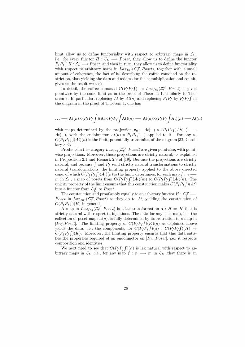
amount of coherence, the fact of its describing the cofree comonad on the re-striction, that yielding the data and axioms for the comultiplication and counit,gives us the result we seek.

In detail, the cofree comonad C(PfPf

∫) on LaxInj(L

opΣ , Poset) is given

pointwise by the same limit as in the proof of Theorem 1, similarly to The-orem 3. In particular, replacing At by At(n) and replacing PfPf by PfPf

∫in

the diagram in the proof of Theorem 1, one has

. . . −→ At(n)×(PfPf

∫)(At×PfPf

∫At)(n) −→ At(n)×(PfPf

∫At)(n) −→ At(n)

with maps determined by the projection π0 : At(−) × (PfPf

∫)At(−) −→

At(−), with the endofunctor At(n) × PfPf

∫(−) applied to it. For any n,

C(PfPf

∫)(At)(n) is the limit, potentially transfinite, of the diagram [32, Corol-

lary 3.3].Products in the category LaxInj(L

opΣ , Poset) are given pointwise, with point-

wise projections. Moreover, those projections are strictly natural, as explainedin Proposition 2.1 and Remark 2.9 of [19]. Because the projections are strictlynatural, and because

∫and Pf send strictly natural transformations to strictly

natural transformations, the limiting property applied to the above directedcone, of which C(PfPf

∫)(At)(n) is the limit, determines, for each map f : n −→

m in LΣ, a map of posets from C(PfPf

∫)(At)(m) to C(PfPf

∫)(At)(n). The

unicity property of the limit ensures that this construction makes C(PfPf

∫)(At)

into a functor from LopΣ to Poset.

The construction and proof apply equally to an arbitrary functor H : LopΣ −→

Poset in LaxInj(LopΣ , Poset) as they do to At, yielding the construction of

C(PfPf

∫)(H) in general.

A map in LaxInj(LopΣ , Poset) is a lax transformation α : H ⇒ K that is

strictly natural with respect to injections. The data for any such map, i.e., thecollection of poset maps α(n), is fully determined by its restriction to a map in[Inj, Poset]. The limiting property of C(PfPf

∫)(K)(n) as explained above

yields the data, i.e., the components, for C(PfPf

∫)(α) : C(PfPf

∫)(H) ⇒

C(PfPf

∫)(K). Moreover, the limiting property ensures that this data satis-

fies the properties required of an endofunctor on [Inj, Poset], i.e., it respectscomposition and identities.

We next need to see that C(PfPf

∫)(α) is lax natural with respect to ar-

bitrary maps in LΣ, i.e., for any map f : n −→ m in LΣ, that there is an

26

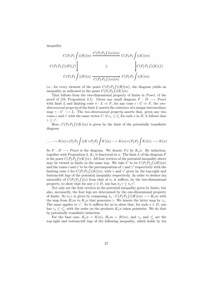
inequality

C(PfPf

∫)(H)(m)

C(PfPf

∫)(α)(m)

✲ C(PfPf

∫)(K)(m)

≥

C(PfPf

∫)(H)(n)

C(PfPf

∫)(H)(f)

❄

C(PfPf

∫)(α)(n)

✲ C(PfPf

∫)(K)(n)

C(PfPf

∫)(K)(f)

❄

i.e., for every element of the poset C(PfPf

∫)(H)(m), the diagram yields an

inequality as indicated in the poset C(PfPf

∫)(K)(n).

That follows from the two-dimensional property of limits in Poset, cf theproof of [19, Proposition 2.1]. Given any small diagram F : D −→ Posetwith limit L and limiting cone π : L ⇒ F , for any cone c : C ⇒ F , the one-dimensional property of the limit L asserts the existence of a unique intermediarymap γ : C −→ L. The two-dimensional property asserts that, given any twocones c and c′ with the same vertex C, if cx ≤ c′x for each x in D, it follows thatγ ≤ γ′.

Here, C(PfPf

∫)(K)(n) is given by the limit of the potentially transfinite

diagram

. . . −→ K(n)×(PfPf

∫)(K×PfPf

∫K)(n) −→ K(n)×(PfPf

∫K)(n) −→ K(n)

So F : D −→ Poset is the diagram. We denote Fx by Kxn. By induction,together with Proposition 2, Kx is functorial in n. The limit L of the diagram Fis the poset C(PfPf

∫)(K)(n). All four vertices of the potential inequality above

may be viewed as limits in the same way. We take C to be C(PfPf

∫)(H)(m)

and the cones c and c′ to be the precomposition of γ and γ′ respectively with thelimiting cone π for C(PfPf

∫)(K)(n), with γ and γ′ given by the top-right and

bottom-left legs of the potential inequality respectively. In order to deduce laxnaturality of C(PfPf

∫)(α) from that of α, it suffices, by the two-dimensional

property, to show that for any x ∈ D, one has πxγ ≤ πxγ′.Not only are the four vertices in the potential inequality given by limits, but

also, necessarily, the four legs are determined by the one-dimensional propertyof limits. So πxγ is given by composing πx : C(PfPf

∫)(H)(m) −→ Hxm with

the map from Hxm to Kxn that generates γ. We denote the latter map by γx.The same applies to γ′. So it suffices for us to show that, for each x ∈ D, onehas γx ≤ γ′

x, with the order on the products Kxn taken pointwise. We do thatby potentially transfinite induction.

For the base case, Kxn = K(n), Hxm = H(m), and γx and γ′x are the

top-right and bottom-left legs of the following inequality, which holds by lax

27

naturality of α:

H(m)α(m)

✲ K(m)

≥

H(n)

H(f)

❄

α(n)✲ K(n)

K(f)

❄

Thus for x = 0, α is a lax transformation from Hx to Kx that we denote by αx.For a successor ordinal, we may assume that αx : Hx ⇒ Kx is lax natural,

and we need to see that we have an inequality in the following diagram:

H(m)× (PfPf

∫Hx)(m)

αx+1(m)✲ K(m)× (PfPf

∫Kx)(m)

≥

H(n)× (PfPf

∫Hx)(n)

H(f)× (PfPf

∫Hx)(f)

❄

αx+1(n)✲ K(n)× (PfPf

∫Kx)(n)

K(f)× (PfPf

∫Kx)(f)

❄

where αx+1 = α × PfPf

∫αx. By Proposition 2,

∫αx is lax natural as

∫is

functorial; composition with Pf is also functorial; and so, αx+1, being a productof two lax natural transformations, is itself lax natural, yielding the inequality.

For a limit ordinal, we have the inequality we seek by a simple applicationof the two-dimensional property applied to the limit of the partial diagram forC(PfPf

∫)(K)(n) up to stage x.

Thus we have defined C(PfPf

∫) as an endofunctor on LaxInj(L

opΣ , Poset).

The counit and comultiplication of C(PfPf

∫) are also constructed by restricting

to [Inj, Poset], using the classical result for the strict setting [32], then using thetwo-dimensional property of the limit to verify coherence in regard to arbitrarymaps in LΣ.

The construction of p is given pointwise, with it following from its coinductiveconstruction that it yields the coinductive trees as required: because of ourconstruction of

∫At to take the place At in Theorem 3, the image of p lies in

PfPf

∫At.

The lax naturality in respect to general maps f : m −→ n means thata substitution applied to an atom A(x1, . . . , xn) ∈ At(n), i.e., application ofthe function At(f) to A(x1, . . . , xn), followed by application of p, i.e., takingthe coinductive tree for the substituted atom, or application of the function(C(PfPf

∫)At)f) to the coinductive tree for A(x1, . . . , xn) potentially yield dif-

ferent trees: the former substitutes into A(x1, . . . , xn), then takes its coinductivetree, while the latter applies a substitution to each node of the coinductive treefor A(x1, . . . , xn), then prunes to remove redundant branches.

28

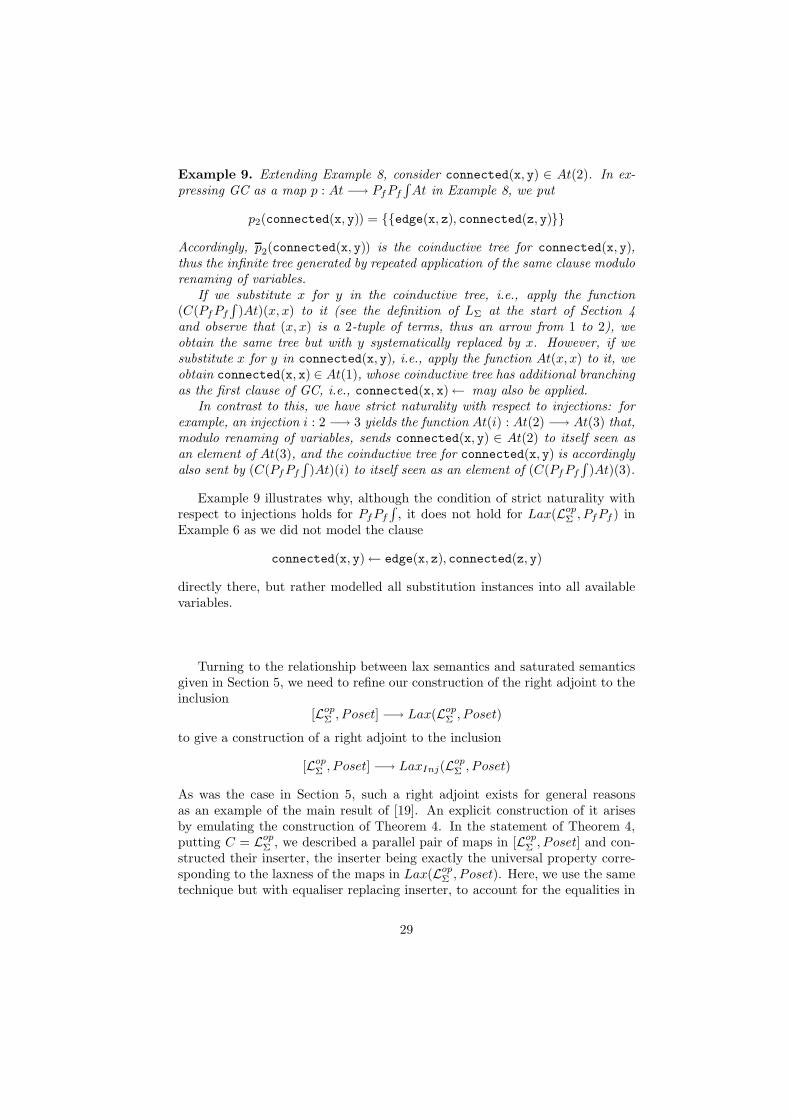
Example 9. Extending Example 8, consider connected(x, y) ∈ At(2). In ex-pressing GC as a map p : At −→ PfPf

∫At in Example 8, we put

p2(connected(x, y)) = {{edge(x, z), connected(z, y)}}

Accordingly, p2(connected(x, y)) is the coinductive tree for connected(x, y),thus the infinite tree generated by repeated application of the same clause modulorenaming of variables.

If we substitute x for y in the coinductive tree, i.e., apply the function(C(PfPf

∫)At)(x, x) to it (see the definition of LΣ at the start of Section 4

and observe that (x, x) is a 2-tuple of terms, thus an arrow from 1 to 2), weobtain the same tree but with y systematically replaced by x. However, if wesubstitute x for y in connected(x, y), i.e., apply the function At(x, x) to it, weobtain connected(x, x) ∈ At(1), whose coinductive tree has additional branchingas the first clause of GC, i.e., connected(x, x)← may also be applied.

In contrast to this, we have strict naturality with respect to injections: forexample, an injection i : 2 −→ 3 yields the function At(i) : At(2) −→ At(3) that,modulo renaming of variables, sends connected(x, y) ∈ At(2) to itself seen asan element of At(3), and the coinductive tree for connected(x, y) is accordinglyalso sent by (C(PfPf

∫)At)(i) to itself seen as an element of (C(PfPf

∫)At)(3).

Example 9 illustrates why, although the condition of strict naturality withrespect to injections holds for PfPf

∫, it does not hold for Lax(Lop

Σ , PfPf ) inExample 6 as we did not model the clause

connected(x, y)← edge(x, z), connected(z, y)

directly there, but rather modelled all substitution instances into all availablevariables.

Turning to the relationship between lax semantics and saturated semanticsgiven in Section 5, we need to refine our construction of the right adjoint to theinclusion

[LopΣ , Poset] −→ Lax(Lop

Σ , Poset)

to give a construction of a right adjoint to the inclusion

[LopΣ , Poset] −→ LaxInj(L

opΣ , Poset)

As was the case in Section 5, such a right adjoint exists for general reasonsas an example of the main result of [19]. An explicit construction of it arisesby emulating the construction of Theorem 4. In the statement of Theorem 4,putting C = Lop

Σ , we described a parallel pair of maps in [LopΣ , Poset] and con-

structed their inserter, the inserter being exactly the universal property corre-sponding to the laxness of the maps in Lax(Lop

Σ , Poset). Here, we use the sametechnique but with equaliser replacing inserter, to account for the equalities in

29

LaxInj(C, Poset). Thus we take an equaliser of two variants of δ1 and δ2 seenas maps in [Lop

Σ , Poset] with domain Ins(δ1, δ2)Again, one may use the same constructions of saturation and desaturation

as before, i.e., use a right Kan extension. However, now, instead of applyingthe right Kan extension to PcPf as in [2], one may apply it to PfPf

∫At. This

still generates countability as application of the right Kan extension generatescountability, but the saturation construction is now applied to an inherentlyfinitary map, p : At −→ PfPf

∫At, rather than to a map with countability

already built into it. So our account of existential variables allows a refinement,albeit a subtle one, to saturated semantics, in addition to refining lax semantics.

7. Semantics for variables in logic programs: local variables

The relationship between the semantics of logic programming we proposehere and that of local state is yet to be explored fully, and we leave the bulkof it to future work. However, as explained in Section 6, the definition of

∫was informed by the semantics for local state in [26], and we have preliminaryresults that strengthen the relationship.

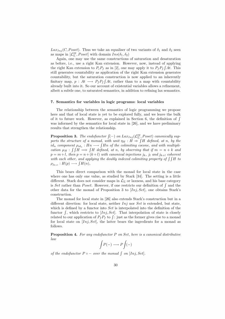
Proposition 3. The endofunctor∫(−) on LaxInj(L

opΣ , Poset) canonically sup-

ports the structure of a monad, with unit ηH : H ⇒∫H defined, at n, by the

idn component ρidn: Hn −→

∫Hn of the colimiting cocone, and with multipli-

cation µH :∫ ∫

H =⇒∫

H defined, at n, by observing that if m = n + k andp = m+ l, then p = n+(k+ l) with canonical injections jk, jl and jk+l coherentwith each other, and applying the doubly indexed colimiting property of

∫ ∫H to

ρjk+l: H(p) −→

∫H(n),

This bears direct comparison with the monad for local state in the casewhere one has only one value, as studied by Stark [34]. The setting is a littledifferent. Stark does not consider maps in LΣ or laxness, and his base categoryis Set rather than Poset. However, if one restricts our definition of

∫and the

other data for the monad of Proposition 3 to [Inj, Set], one obtains Stark’sconstruction.

The monad for local state in [26] also extends Stark’s construction but in adifferent direction: for local state, neither Inj nor Set is extended, but state,which is defined by a functor into Set is interpolated into the definition of thefunctor

∫, which restricts to [Inj, Set]. That interpolation of state is closely

related to our application of PfPf to∫

: just as the former gives rise to a monadfor local state on [Inj, Set], the latter bears the ingredients for a monad asfollows.

Proposition 4. For any endofunctor P on Set, here is a canonical distributivelaw ∫

P (−) −→ P

∫(−)

of the endofunctor P ◦ − over the monad∫

on [Inj, Set].

30

The canonicity of the distributive law arises as∫

is defined pointwise as acolimit, and the distributive law is the canonical comparison map determinedby applying P pointwise to the colimiting cone defining

∫.

The functor PfPf does not quite satisfy the axioms for a monad [35] (seealso [2]), but variants of PfPf , in particular PfMf , where Mf is the finite mul-tiset monad on Set, do [35] (also see [2]). Putting P = PfMf , the distributivelaw of Proposition 4 respects the monad structure of PfMf , yielding a canonicalmonad structure on the composite PfMf

∫.

The full implications of that are yet to be investigated, but, trying to emulatethe analysis of local state in [26], we believe we have a natural set of operationsand equations that generate the monad PfMf

∫. That encourages us consider-

ably towards the possibility of seeing the semantics for logic programming, bothlax and saturated, as an example of a general semantics of local effects. We havenot yet fully understood the significance of the specific combination of opera-tions and equations generating the monad, but we are currently investigatingit.

8. Conclusions and Further Work

Let Pf be the covariant finite powerset functor on Set. Then, to give avariable-free logic program P is equivalent to giving a PfPf -coalgebra structurep : At −→ PfPfAt on the set At of atoms in the program. Now let C(PfPf )be the cofree comonad on PfPf . Then, the C(PfPf )-coalgebra p : At −→C(PfPf )At corresponding to p sends an atom to the coinductive tree it gener-ates. This fact is the basis for both our lax semantics and Bonchi and Zanasi’ssaturated semantics for logic programming.

Two problems arise when, following standard category theoretic practice, onetries to extend this semantics to model logic programs in general by extendingfrom Set to [Lop

Σ , Set], where LΣ is the free Lawevere theory generated by asignature Σ. The first is that the natural construction p : At −→ PfPfAt doesnot form a natural transformation, so is not a map in [Lop

Σ , Set].Two resolutions were proposed to that: lax semantics [1], which we have

been developing in the tradition of semantics for data refinement [21], and sat-urated semantics [2], which Bonchi and Zanasi have adopted. In this paper, wehave shown that the two resolutions are complementary rather than competing,the first modelling the theorem-proving aspect of logic programming, while thelatter models proof search.

In modelling theorem-proving, lax semantics led us to identify and developthe notion of coinductive tree. To express the semantics, we extended [Lop

Σ , Set]to Lax(Lop

Σ , Poset), the category of strict functors and lax transformations be-tween them. We followed standard semantic practice in extending Pf from Setto Poset and we postcomposed the functor At : Lop

Σ −→ Poset by PfPf . Bonchiand Zanasi also postcomposed At by PfPf , but then saturated. We showed thattheir saturation and desaturation constructions are generated exactly by start-ing from Lax(Lop

Σ , Poset) rather than from [ob(LΣ)op, Set] as they did, thus

31

unifying the underlying mathematics of the two developments, supporting theircomputational coherence.

The second problem mentioned above relates to existential variables, thosebeing variables that appear in the antecedent of a clause but not in its head.The problem of existential clauses is well-known in the literature on theoremproving and within communities that use term-rewriting, TM-resolution or theirvariants. In TRS [29], existential variables are not allowed to appear in rewritingrules, and in type inference, the restriction to non-existential programs is com-mon [31]. In logic programming, the problem of handling existential variableswhen constructing proofs with TM-resolution marks the boundary between itstheorem-proving and problem-solving aspects.

Existential variables are not present in many logic programs, but they dooccasionally occur in important examples, such as those developed by Sterlingand Shapiro [27]. The problem for us was that, in the presence of existentialvariables, the natural model p : At −→ PfPfAt of a logic program mightescape its codomain, i.e., pn(A) might not lie in PfPfAt(n) because of thenew variables. On one hand, we want to model them, but on the other, the factof the difficulty for us means that we have semantically identified the conceptof existential variable, which is positive.

In this paper, we have resolved the problem by refining Lax(LopΣ , Poset) to

LaxInj(LopΣ , Poset), insisting upon strict naturality for injections, and by refin-

ing the construction PfPfAt to PfPf

∫At, thus allowing for additional variables

in the tail of a clause in a logic program. That has allowed us to model coinduc-tive trees for arbitrary logic programs, in particular those including existentialvariables. We have also considered the effect of such refinement on saturatedsemantics, where the right Kan extension generates countability but use of Pc

is no longer required.In order to refine PfPf (−), we followed a technique developed in the seman-

tics of local state [26]. That alerted us to the relationship between variablesin logic programming with the use of worlds in modelling local state. So, asongoing work, we are now relating our semantics for logic programming withthat for local state. For the future, we shall continue to develop that, withthe hope of being able to locate our semantics of logic programming within ageneral semantics for local effects.

Beyond that, a question that we have not considered semantically at allyet but which our applied investigations are encouraging is that of modellingrecursion. There are fundamentally two kinds of recursion that arise in logicprogramming as there may be recursion in terms and recursion in proofs. Forexample, stream(scons(x, y))← stream(y) is a standard (co-)recursive defini-tion of infinite streams in logic programming literature. More abstractly, thefollowing program P1: p(f(x))← p(x) defines an infinite data structure p withconstructor f . For such cases, proofs given by coinductive trees will be finite.An infinite sequence of (finite) coinductive trees will be needed to approxi-mate the intended operational semantics of such a program, as we discuss indetail in [1, 36]. In contrast, there are programs like P2: p(x)← p(x) or P3:p(x)← p(f(x)) that are also recursive, but additionally their proofs as given by

32

coinductive trees will have an infinite size.In [37, 38] programs like P1 were called productive, for producing (infinite)

data, and programs like P2 and P3 – non-productive, for recursing withoutproducing substitutions. The productive case amounts to a loop in the Lawveretheory LΣ [39], while the non-productive case amounts to repetition withina coinductive tree, possibly modulo a substitution. This paper gives a closeanalysis of trees. That should set the scene for investigation of recursion, as itseems likely to yield more general kinds of graph that arise by identifying loopsin LΣ and by equating nodes in trees.

The lax semantics we presented here has recently inspired investigationsinto the importance of TM-resolution (as modelled by the coinductive trees)in programming languages. In particular, TM-resolution is used in type classinference in Haskell [31]. In [13, 40] we showed applications of nonterminatingTM-resolution in Haskell type classes. We plan to continue looking for applica-tions of this work in programming language design beyond logic programming.

Acknowledgements

Ekaterina Komendantskaya would like to acknowledge the support of EPSRCGrant EP/K031864/1-2. John Power would like to acknowledge the support ofEPSRC grant EP/K028243/1 and Royal Society grant IE151369. We both ac-knowledge the support of LMS grant SC7-1617-10, which facilitated the writingof this paper.

Bibliography

[1] E. Komendantskaya, J. Power, M. Schmidt, Coalgebraic logic program-ming: from semantics to implementation, J. Log. Comput. 26 (2) (2016)745 – 783.

[2] F. Bonchi, F. Zanasi, Bialgebraic semantics for logic programming, LogicalMethods in Computer Science 11 (1) (2015) 1–47.

[3] G. Kelly, Basic concepts of enriched category theory, Vol. 64, CambridgeUniversity Press, 1982.

[4] G. Gupta, V. Costa, Optimal implementation of and-or parallel prolog, in:PARLE’92, 1994, pp. 71 – 92.

[5] R. Bruni, U. Montanari, F. Rossi, An interactive semantics of logic pro-gramming, TPLP 1 (6) (2001) 647 – 690.

[6] F. Bonchi, U. Montanari, Reactive systems, (semi-)saturated semantics andcoalgebras on presheaves, Theor. Comput. Sci. 410 (41) (2009) 4044 – 4066.

[7] M. Comini, G. Levi, M. C. Meo, A theory of observables for logic programs,Inf. Comput. 169 (1) (2001) 23 – 80.

33

[8] J. Lloyd, Foundations of Logic Programming, Springer-Verlag, 1987.

[9] E. Komendantskaya, G. McCusker, J. Power, Coalgebraic semantics forparallel derivation strategies in logic programming, in: AMAST’2010, Vol.6486 of Lecture Notes in Computer Science, Springer, 2011, pp. 111 – 127.

[10] E. Komendantskaya, M. Schmidt, J. Heras, Exploiting parallelism in coal-gebraic logic programming, Electr. Notes Theor. Comput. Sci. 303 (2014)121 – 148.

[11] P. Johann, E. Komendantskaya, V. Komendantskiy, Structural resolutionfor logic programming, in: Proceedings of the Technical Communicationsof the 31st International Conference on Logic Programming (ICLP 2015),Cork, Ireland, August 31 - September 4, 2015., Vol. 1433 of CEUR Work-shop Proceedings, 2015.

[12] P. Fu, E. Komendantskaya, A type-theoretic approach to resolution, in:Logic-Based Program Synthesis and Transformation - 25th InternationalSymposium, LOPSTR 2015, Siena, Italy, July 13-15, 2015. Revised SelectedPapers, Vol. 9527 of Lecture Notes in Computer Science, Springer, 2015,pp. 91 – 106.

[13] P. Fu, E. Komendantskaya, T. Schrijvers, A. Pond, Proof relevant corecur-sive resolution, in: Functional and Logic Programming - 13th InternationalSymposium, FLOPS 2016, Kochi, Japan, March 4-6, 2016, Proceedings,Vol. 9613 of Lecture Notes in Computer Science, Springer, 2016, pp. 126 –143.

[14] F. Bonchi, F. Zanasi, Saturated semantics for coalgebraic logic program-ming, in: Algebra and Coalgebra in Computer Science - 5th InternationalConference, CALCO 2013, Warsaw, Poland, September 3-6, 2013. Proceed-ings, Vol. 8089 of Lecture Notes in Computer Science, Springer, 2013, pp.80 – 94.

[15] G. Amato, J. Lipton, R. McGrail, On the algebraic structure of declarativeprogramming languages, Theor. Comput. Sci. 410 (46) (2009) 4626 – 4671.

[16] Y. Kinoshita, A. J. Power, A fibrational semantics for logic programs, in:Extensions of Logic Programming, 5th International Workshop, ELP’96,Leipzig, Germany, March 28-30, 1996, Proceedings, Vol. 1050 of LectureNotes in Computer Science, Springer, 1996, pp. 177 – 191.

[17] E. Komendantskaya, J. Power, Coalgebraic semantics for derivations inlogic programming, in: Algebra and Coalgebra in Computer Science -4th International Conference, CALCO 2011, Winchester, UK, August 30 -September 2, 2011. Proceedings, Vol. 6859 of Lecture Notes in ComputerScience, Springer, 2011, pp. 268 – 282.

[18] J. Benabou, Introduction to bicategories, Lecture Notes in Mathematics 47(1967) 1 – 77.

34

[19] R. Blackwell, G. Kelly, A. Power, Two-dimensional monad theory, J. PureAppl. Algebra 59 (1989) 1 – 41.

[20] G. Kelly, Coherence theorems for lax algebras and for distributive laws, in:Category seminar, Vol. 420 of Lecture Notes in Mathematics, Spriniger,1974, pp. 281 – 375.

[21] J. He, C. A. R. Hoare, Categorical semantics for programming languages,in: Mathematical Foundations of Programming Semantics, 5th Interna-tional Conference, Tulane University, New Orleans, Louisiana, USA, March29 - April 1, 1989, Proceedings, Vol. 442 of Lecture Notes in Computer Sci-ence, Springer, 1989, pp. 402 – 417.

[22] H. Jifeng, C. Hoare, Data refinement in a categorical setting, Tech. Rep.Technical Monograph PRG-90, Oxford University Computing Laboratory,Programming Research Group, Oxford (1990).

[23] Y. Kinoshita, A. Power, Lax naturality through enrichment, J. Pure Appl.Algebra 112 (1996) 53 – 72.

[24] A. J. Power, An algebraic formulation for data refinement, in: Mathemati-cal Foundations of Programming Semantics, 5th International Conference,Tulane University, New Orleans, Louisiana, USA, March 29 - April 1, 1989,Proceedings, Vol. 442 of Lecture Notes in Computer Science, Springer,1989, pp. 390 – 401.

[25] E. Komendantskaya, J. Power, Category theoretic semantics for theoremproving in logic programming: Embracing the laxness, in: CoalgebraicMethods in Computer Science - 13th IFIP WG 1.3 International Workshop,CMCS 2016, Colocated with ETAPS 2016, Eindhoven, The Netherlands,April 2-3, 2016, Revised Selected Papers, Vol. 9608 of Lecture Notes inComputer Science, Springer, 2016, pp. 94 – 113.

[26] G. D. Plotkin, J. Power, Notions of computation determine monads, in:Foundations of Software Science and Computation Structures, 5th Inter-national Conference, FOSSACS 2002. Held as Part of the Joint EuropeanConferences on Theory and Practice of Software, ETAPS 2002 Grenoble,France, April 8-12, 2002, Proceedings, Vol. 2303 of Lecture Notes in Com-puter Science, Springer, 2002, pp. 342 – 356.

[27] L. Sterling, E. Shapiro, The art of Prolog, MIT Press, 1986.

[28] E. Komendantskaya, J. Power, Coalgebraic derivations in logic program-ming, in: Computer Science Logic, 25th International Workshop / 20th An-nual Conference of the EACSL, CSL 2011, September 12-15, 2011, Bergen,Norway, Proceedings, Vol. 12 of LIPIcs, Schloss Dagstuhl - Leibniz-Zentrumfuer Informatik, 2011, pp. 352 – 366.

[29] Terese, Term Rewriting Systems, Cambridge University Press, 2003.

35

[30] L. Simon, A. Bansal, A. Mallya, G. Gupta, Co-logic programming: Ex-tending logic programming with coinduction, in: Automata, Languagesand Programming, 34th International Colloquium, ICALP 2007, Wroclaw,Poland, July 9-13, 2007, Proceedings, Vol. 4596 of Lecture Notes in Com-puter Science, Springer, 2007, pp. 472 – 483.

[31] S. P. Jones, M. Jones, E. Meijer, Type classes: An exploration of the designspace, in: Haskell Workshop, 1997.

[32] J. Worrell, Terminal sequences for accessible endofunctors, Electr. NotesTheor. Comput. Sci. 19 (1999) 24 – 38.

[33] S. MacLane, Categories for the Working Mathematician, Graduate Textsin Mathematics, Springer, 1971.

[34] I. Stark, Categorical models for local names, Lisp and Symbolic Computa-tion 9 (1) (1996) 77 – 107.

[35] M. Hyland, M. Nagayama, J. Power, G. Rosolini, A category theoreticformulation for engeler-style models of the untyped lambda, Electr. NotesTheor. Comput. Sci. 161 (2006) 43 – 57.

[36] P. Johann, E. Komendantskaya, Structural resolution: a framework forcoinductive proof search and proof construction in horn clause logic,Draft.Arxiv.org/abs/1707.01541.

[37] E. Komendantskaya, P. Johann, M. Schmidt, A productivity checker forlogic programming, in: Logic-Based Program Synthesis and Transforma-tion - 26th International Symposium, LOPSTR 2016, Edinburgh, UK,September 6-8, 2016, Revised Selected Papers, Vol. 10184 of Lecture Notesin Computer Science, Springer, 2017, pp. 168–186.

[38] P. Fu, E. Komendantskaya, Operational semantics of resolution and pro-ductivity in horn clause logic, Formal Asp. Comput. 29 (3) (2017) 453–474.

[39] E. Komendantskaya, Y. Li, Productive corecursion in logic programming,Journal of Theory and Practice of Logic Programming. International Con-ference on Logic Programming (ICLP’17).

[40] F. Farka, E. Komendantskaya, K. Hammond, Coinductive soundness ofcorecursive type class resolution, in: Logic-Based Program Synthesis andTransformation - 26th International Symposium, LOPSTR 2016, Edin-burgh, UK, September 6-8, 2016, Revised Selected Papers, Vol. 10184 ofLecture Notes in Computer Science, Springer, 2017, pp. 311–327.

36