logic gate delay modeling -iii bishnu prasad das research scholar cedt, iisc, bangalore...
TRANSCRIPT

Logic Gate Delay Modeling -III
Bishnu Prasad Das
Research Scholar
CEDT, IISc, Bangalore
OUTLINE
• Delay Model History
• Static Timing Analysis (STA)
• Corner Models
• Drawback of Corner Approach
• Statistical Static Timing Analysis(SSTA)
• Summary

Delay Model History
Courtesy : Synopsys

What to do with Delay Models?
• Timing analysis of the whole chip
Problem: Given a circuit, find the path(s) with the largest delay (critical paths)
Timing Analysis
• Solution: run SPICE and report the results of the simulation
• Problem: SPICE is computationally expensive to run except for small-size circuits• WANTED: We need a fast method that produces relatively accurate timing
results compared to SPICE

Combinational Blocks
• Arrival time in Green
• Interconnect delay in Red
• Gate Delay in Blue• What is the right mathematical object to represent this physical objects ?

Combinational Blocks as DAG
Use a labeled directed acyclic graph G = <V,E>
Vertices represent
gates, primary inputs
and primary outputs
Edges represent wires
Labels represent delays
Now what do we do with this?
Static timing analysis
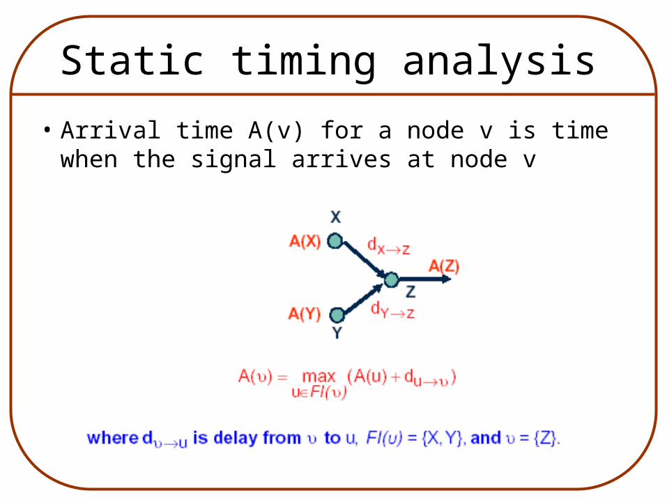
• Arrival time A(v) for a node v is time when the signal arrives at node v

Static timing analysis
1/2
2/43/5
1/22/4
2/3
1/2
I1
I2
I3
I4
I5
I6
O1
O2
C17 from ISCAS’85 benchmarks
All inputs are arrive at time 0
Assuming all interconnects have 0 delay
Each gate has rise/fall delay
1/2
2/4
1/2
7/7
5/4
9/10
9/11
slack = arrival time – required arrival time paths with negative slacks need to be
eliminated!
criticalpath

STA can lead to false critical paths
21MUX
delay = 5
delay = 3
delay = 5
delay = 3
21MUX
outa
b
0
1 1
0
• What is critical path delay according to STA?
• Is this path realizable?No, actual delay is less than estimated by STA
STA assumes a signal would propagate from a gate input to its output regardless of the values of other inputs
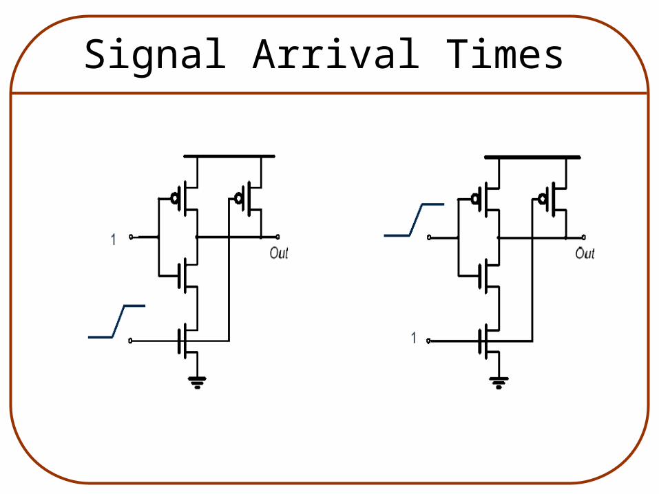
Signal Arrival Times

Simultaneous Arrival Times

Simultaneous Arrival Times

Limitations of STA
• False path
• Simultaneous Arrival Time
• STA is done across all corners (Computationally Expensive)

Corner Models
• Four types of Corner models– Fast Corner
– Slow Corner
– Slow NMOS Fast PMOS
– Fast NMOS Slow PMOS
– Typical Corner

Design Corners
Slow Fast
NMOS
Slo
wF
ast
PM
OS
SS FS
FSFF
TT
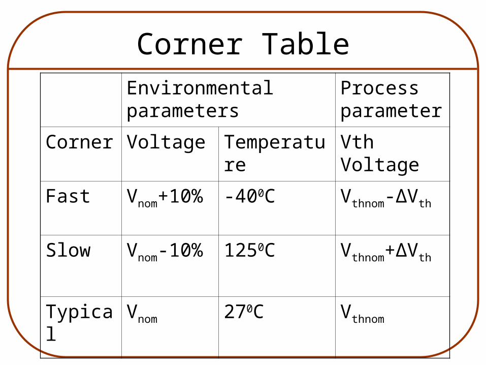
Corner TableEnvironmental parameters Process
parameter
Corner Voltage Temperature Vth Voltage
Fast Vnom+10% -400C Vthnom-ΔVth
Slow Vnom-10% 1250C Vthnom+ΔVth
Typical Vnom 270C Vthnom

Applications of Corners
• For Power and race condition like hold time use Fast corner
• For Delay simulation use Slow corner
• The other two corners are used for circuits which require precise sizing for proper functioning. Ex: Memory and pseudo NMOS circuit.
Limitations of Corner Models
• Worst case assumption is insignificant
• This leads to over design
• Hence more power, area and loss of performance
• Need more intelligent accounting of variations

Gate Length Variation
[Orshansky, et. al, IEEE Trans. On Sem. Manufacturing, Feb 2004]

Environmental Variations: Vdd
[Anirudh Devgan, IBM, Mar 05]
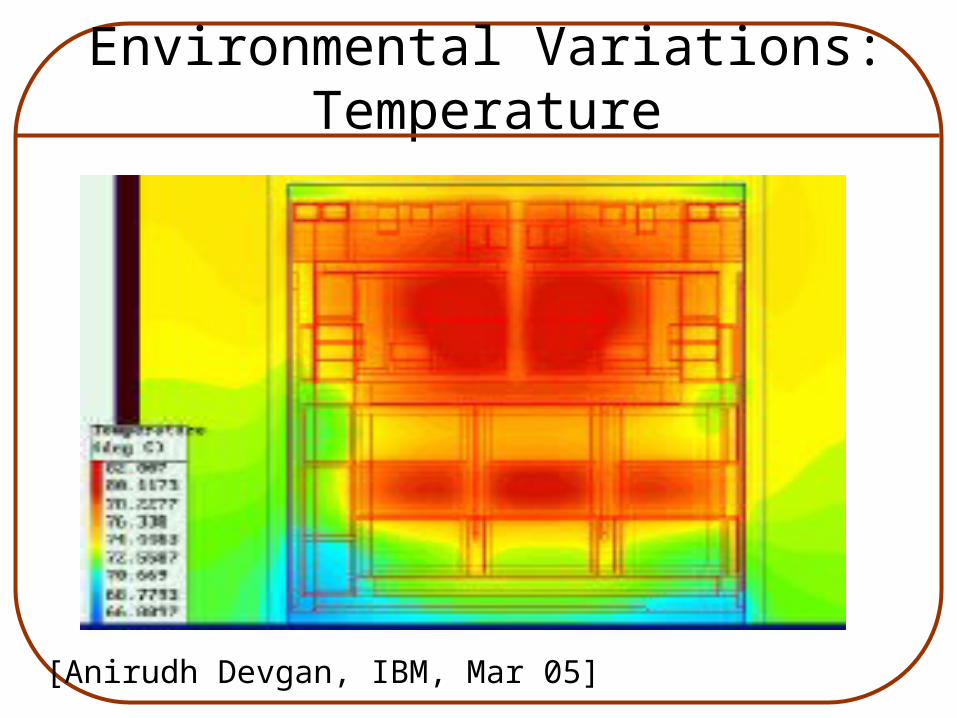
Environmental Variations: Temperature
[Anirudh Devgan, IBM, Mar 05]

Statistical Static Timing Analysis
i
j
oAi
Aj
Ao
Ao = max(Ai+ Dio , Aj+ Djo)
Delay is no longer Deterministic, it is a random variable

Addition Operation
• Addition operation: The sum of two random number is convolutions of their probability functions.
Ao = Ai+ Dio
Where Ci is the CDF of Ai .
Pio is the PDF of Dio.
d ioPt
tiCoC 0

Max Operation
• Max Operation: The CDF of the maximum of two independent random variables is simply the product of the CDF of two variables
Ao = Max ( Ai , Aj )
• The CDF of node “o” is given by Co(t) = Ci(t) Cj(t)
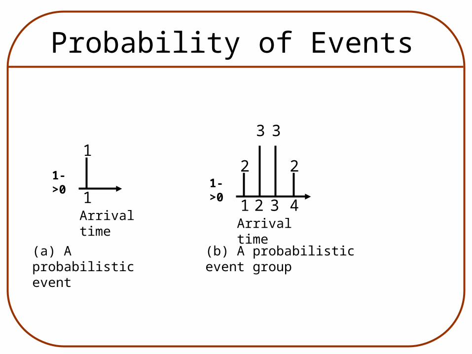
Probability of Events
1
1
1->0
Arrival time
(a) A probabilistic event
1
21->0
Arrival time
2
3 3
2 3 4
(b) A probabilistic event group

Propagating a Single event
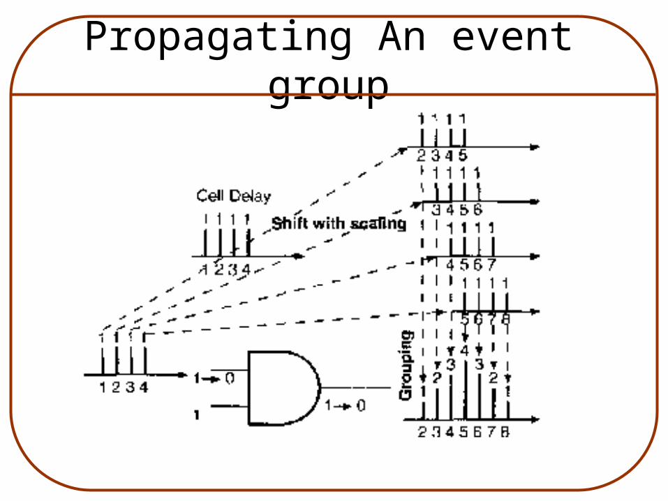
Propagating An event group

Output of SSTA
p df
delay
I1
I2
I3
I4
I5
I6
O1
O2
p df
delay
p df
delay
?
y
z
C17 ISCAS Benchmark
Summary
• Static Timing Analysis
• Limitations of STA
• Corner Models
• Limitations of Corner Models in Presence of Process Variation
• Statistical Static Timing Analysis

References
• For SSTA:• J. J. Liou et.al, “Fast Statistical Timing Analysis by Probabilistic Event
Propagation”, DAC pp. 661-666, June 2001.• A. Devgan and C. Kashyap, “Block-based Timing Analysis with
Uncertainty,” ICCAD, pp. 607-614, Nov. 2003.• H.Chang, V. Zolotov, S. Narayan and C. Visweswariah, “Parameterized
Block-Based Statistical Timing analysis with Non-Gaussian Parameters, Nonlinear Delay Functions,” DAC, pp. 71-76, June 2005.
• For Corner Model:• N. H. E. Weste and D. Harris, “CMOS VLSI Design, A circuits and
Systems Perspective” 3rd edition
References• Go to solvnet site
https://solvnet.synopsys.com/amserver/UI/Login and do an account for these materials • CCS Models Xin Bao, Khusro Sajid, Elisabeth Moseley,
“Timing Sign-off using CCS Libraries at Qualcomm”, Snug 2006 San Jose
Peter Chih-Yang Pong, Steve H. Tsai, “An Investigation of CCS”, Snug Taiwan 2006
CCS Timing Library Characterization Guidelines