log-linear interpolation of language models · log-linear interpolation of language models...
TRANSCRIPT

Log-Linear Interpolation of
Language Models
Alexander GutkinPeterhouse
University of Cambridge
19th November 2000
Thesis submitted to the University of Cambridge in partial fulfilment of the
requirements for the degree of
Master of Philosophy
in
Computer Speech and Language Processing

Abstract
Building probabilistic models of language is a central task in natural language andspeech processing allowing to integrate the syntactic and/or semantic (and recentlypragmatic) constraints of the language into the systems. Probabilistic languagemodels are an attractive alternative to the more traditional rule-based systems,such as context free grammars, because of the recent availability of massive amountof text corpora which can be used to efficiently train the models and because insteadof binary grammaticality judgement offered by the rule-based systems, likelihood ofany sequence of lexical units can be obtained, which is a crucial factor in such tasksas speech recognition. Probabilistic language models also find their application inpart-of-speech tagging, machine translation, semantic disambiguation and numerousother fields.
The most widely used language models are based on the estimation of the proba-bility of observing a given lexical unit conditioned on the observations of n−1 preced-ing lexical units, and are known as n-gram models. When the n-gram estimates arepoor, whatever the reason for that may be, a technique called smoothing is appliedto adjust the estimates and hopefully produce more accurate model. Smoothingtechniques may be roughly divided into the backing-off and interpolation. In thefirst case, the best n-gram model in the current context is selected, whereas in thesecond case all the n-gram models of different specificities are combined together toform a better predictor.
In this thesis, a recently proposed novel interpolation scheme is investigated,namely, the log-linear interpolation. Unlike the original publication, however, whichdealt with combining the models of unrelated nature, the aim of this thesis is toformulate the theoretical framework for smoothing the n-gram probability estimatesobtained from similar language models with different levels of specificity on the samecorpus, which will be called log-linear n-gram smoothing, and compare it to thewell-established linear interpolation and back-off methods. The framework beingproposed includes probability combination, parameter optimisation, dealing withdata sparsity and parameter clustering.
The resulting technique is shown to outperform the conventional linear interpo-lation and back-off techniques when applied to the n-gram smoothing tasks.
ii

Acknowledgements
First and foremost I would like to thank my supervisor, Dr Thomas Niesler whohas encouraged, supported and guided my language modelling endeavours duringevery step of the way and without whose sound and friendly advice completion ofthis dissertation would not be possible. My deepest professional gratitude goes tohim.
I owe gratitude to William Lee of Department of Earth Sciences for proofread-ing this thesis and making several insightful comments on mathematical aspects ofpresentation without which this thesis would not appear as it appears now, and toValerie Dorrzapf of Department of English and Applied Linguistics, who suppliedinteresting insights on the things I have been doing from the theoretical linguisticsperspective.
Completion of the experiments described herein has been made possible byPatrick Gosling who continues to maintain excellent facilities for the Speech Grouphere at Fallside Laboratory.
I would also like to thank people who first introduced me to language modellingin speech and natural language processing, namely Dr Ted Briscoe for his excellentcourse of lectures on stochastic context free and unification based grammars andPhil Woodland for his expert professional coverage of language modelling for speechrecognition, as well as following people, postgraduates and members of staff alike,Dr. Mark Gales, Aurelien Max, Paolo Mendonca, Dan Povey, Nathan Smith, andMatt Stuttle, whose friendly attitude and high expertise proved to be a deeplyrewarding experience for me. I want to thank Dr Stephen Pulman for explainingto me the intricate differences between mathematical and computational linguisticsand pointing at the inherent difficulties in the existing approaches.
Finally, it would be unfair not to mention Simon Redhead and Kathrin Schodeland thank them for all those numerous coffee/tobacco breaks and laughs on thebalcony regardless of the time and weather conditions, whose excellent companyhas helped me to enjoy my life in Cambridge, and thank Pal Hegedus and RekaLimbek for everything.
iii

Declaration
This dissertation is the result of my own original work, and where it draws on thework of others, this is acknowledged at the appropriate points in the text. Thisdissertation has not been submitted in whole or in part for a degree at any otherinstitution. The length of this thesis, including footnotes, is approximately 14,815words. The implementation of the theoretical frameworks and algorithms derived inthis work can be found in appendix to this dissertation which is submitted separately.
iv

To my family.

Contents
1 Introduction 1
1.1 Scope of the Thesis . . . . . . . . . . . . . . . . . . . . . . . . . . . . 21.2 Thesis Organisation . . . . . . . . . . . . . . . . . . . . . . . . . . . 3
2 Background to Language Modelling 4
2.1 Equivalence Classification of History . . . . . . . . . . . . . . . . . . 42.2 Statistical Estimation . . . . . . . . . . . . . . . . . . . . . . . . . . 5
2.2.1 Maximum Likelihood estimation . . . . . . . . . . . . . . . . 62.2.2 Sparse data problem . . . . . . . . . . . . . . . . . . . . . . . 7
2.3 Quality Assessment of Language Models . . . . . . . . . . . . . . . . 9
3 Overview of Smoothing Techniques 12
3.1 Discounting Methods . . . . . . . . . . . . . . . . . . . . . . . . . . . 123.1.1 Basic discounting . . . . . . . . . . . . . . . . . . . . . . . . . 123.1.2 Good–Turing estimate . . . . . . . . . . . . . . . . . . . . . . 133.1.3 Cross-validation (deleted estimation) . . . . . . . . . . . . . . 143.1.4 Unconstrained discounting model . . . . . . . . . . . . . . . . 153.1.5 Leaving-one-out estimate for joint probabilities . . . . . . . . 16
3.2 Combination of Estimators . . . . . . . . . . . . . . . . . . . . . . . 183.2.1 Katz’s backing-off . . . . . . . . . . . . . . . . . . . . . . . . 183.2.2 Linear discounting . . . . . . . . . . . . . . . . . . . . . . . . 203.2.3 Absolute discounting . . . . . . . . . . . . . . . . . . . . . . . 203.2.4 Kneser-Ney smoothing . . . . . . . . . . . . . . . . . . . . . . 213.2.5 Linear interpolation . . . . . . . . . . . . . . . . . . . . . . . 213.2.6 Unified view on backing-off and linear interpolation . . . . . 223.2.7 Parameter tying . . . . . . . . . . . . . . . . . . . . . . . . . 23
4 Interpolation of Language Models 25
4.1 Linear Smoothing . . . . . . . . . . . . . . . . . . . . . . . . . . . . . 254.1.1 Parameter tying . . . . . . . . . . . . . . . . . . . . . . . . . 264.1.2 Parameter optimisation . . . . . . . . . . . . . . . . . . . . . 27
4.2 Log-Linear Smoothing . . . . . . . . . . . . . . . . . . . . . . . . . . 294.2.1 Formal framework . . . . . . . . . . . . . . . . . . . . . . . . 314.2.2 Parameter Tying . . . . . . . . . . . . . . . . . . . . . . . . . 324.2.3 Multidimensional optimisation . . . . . . . . . . . . . . . . . 334.2.4 Similarity to Maximum Entropy models . . . . . . . . . . . . 354.2.5 Significance of log-linear interpolation weights . . . . . . . . . 37
vi

CONTENTS vii
5 Performance Evaluation 40
5.1 Language Modelling Corpora . . . . . . . . . . . . . . . . . . . . . . 405.1.1 Transcriptions of Conversational Telephone Speech . . . . . . 405.1.2 The Wall Street Journal (WSJ) Corpus . . . . . . . . . . . . 41
5.2 Baseline Models . . . . . . . . . . . . . . . . . . . . . . . . . . . . . . 425.3 Linear Interpolation . . . . . . . . . . . . . . . . . . . . . . . . . . . 435.4 Log-Linear Interpolation . . . . . . . . . . . . . . . . . . . . . . . . . 45
5.4.1 Performance on Hub5 1997/1998 evaluation sets . . . . . . . 455.4.2 Performance on 1987–1989 WSJ evaluation sets . . . . . . . . 48
5.5 Discussion . . . . . . . . . . . . . . . . . . . . . . . . . . . . . . . . . 51
6 Summary and Conclusion 53
Bibliography 54

List of Tables
5.1 Hub5 language modelling corpus details (sizes of the corpora areshown in total number of words). . . . . . . . . . . . . . . . . . . . . 41
5.2 WSJ language modelling corpus details (sizes of the corpora areshown in total number of words). . . . . . . . . . . . . . . . . . . . . 42
5.3 Total number of words in the kept and held-out portions of thetraining data for Hub5-Train00 and WSJ-Train88 together with thewordlist sizes. . . . . . . . . . . . . . . . . . . . . . . . . . . . . . . . 42
5.4 Perplexities of the baseline back-off models trained on 2000 Hub5language model training data and on 1988 WSJ training data, testedon the respective evaluation sets. . . . . . . . . . . . . . . . . . . . . 43
5.5 Performance of the linear interpolation models (maximum likelihoodand back-off estimates) with clustering constraint of Nmin = 104 andback-off language model on the two test sets from Hub5. . . . . . . . 45
5.6 Perplexity of log-linear smoothing model built on 2000 Hub5 languagemodelling data using Nmin = 104 versus its linear counterpart. . . . . 46
5.7 Optimal linear and log-linear interpolation weights trained on 2000Hub5 language model training corpus with Nmin = 106, with thepair of interpolation weights corresponding to bigram model, and the3-tuple to the trigram model. . . . . . . . . . . . . . . . . . . . . . . 48
5.8 Total number of optimal log-linear smoothing weights calculated foreach level of all the log-linear trigram language models trained duringthe experiments against the total number of optimal weights whoseabsolute values exceeded unity for Hub5 1997/1998 language modelevaluation sets. . . . . . . . . . . . . . . . . . . . . . . . . . . . . . . 49
5.9 Optimal linear and log-linear interpolation weights trained on 1988WSJ language model training corpus with Nmin = 107, with the pairof interpolation weights corresponding to bigram model, and the 3-tuple to the trigram model. . . . . . . . . . . . . . . . . . . . . . . . 49
5.10 Performance of the log-linear smoothing model built on 1988 WSJlanguage modelling data using versus its back-off and linear counter-parts (best models, in terms of the clustering criterion) were selected). 49
5.11 Value of clustering parameter Nmin for which the optimal perplexitiesare obtained on the three WSJ evaluation sets for linear and log-linearinterpolation models. . . . . . . . . . . . . . . . . . . . . . . . . . . . 51
viii

List of Figures
2.1 Rank-frequency plot of the words (unigrams) on doubly logarithmicaxes for small evaluation and big training corpora showing the samepattern of underlying Zipfian distribution. . . . . . . . . . . . . . . . 8
4.1 Plot of the unnormalised log-linear interpolation term as function ofprobability P with the weight values λ being taken from differentranges. . . . . . . . . . . . . . . . . . . . . . . . . . . . . . . . . . . . 38
4.2 Unnormalised log-linear interpolation term surface as a function ofboth the probability P and the log-linear weight λ. . . . . . . . . . . 39
5.1 Influence of cluster size Nmin on the performance of linear interpola-tion of maximum likelihood estimates. . . . . . . . . . . . . . . . . . 43
5.2 Influence of cluster size Nmin on the performance of linear interpola-tion of Katz back-off models. . . . . . . . . . . . . . . . . . . . . . . 44
5.3 Influence of cluster size Nmin on the performance of log-linear inter-polation of Katz back-off estimates on the Hub5 1997/1998 languagemodelling evaluation sets. . . . . . . . . . . . . . . . . . . . . . . . . 46
5.4 Influence of the size of the kept portion of 2000 Hub5 training set onthe performance of linearly and log-linearly smoothed Katz back-offestimates. . . . . . . . . . . . . . . . . . . . . . . . . . . . . . . . . . 47
5.5 Performance of trigram log-linear and linear interpolation models on1987/88/89 WSJ evaluation sets. . . . . . . . . . . . . . . . . . . . . 50
ix
CHAPTER 1
Introduction
Language modelling is the attempt to characterise, capture and exploit syntactic, se-mantic and pragmatic regularities exhibited by natural language. It is being widelyused in many domains including speech recognition, optical character recognition,handwriting recognition, machine translation, part-of-speech tagging, dialog mod-elling and spelling correction. In its simplest form, a language model may be arepresentation of the list of the sentences belonging to a language, while the morecomplex models may also try to describe the structure and meaning underlying thesentences in a natural language.
Techniques for modelling the language historically fall into two categories. Thefirst type of models are the traditional grammars, such as context free and unificationbased grammars, which although being rigorously defined from linguistic perspec-tive, suffer from the typical deficiencies of the rule-based systems. They are difficultto maintain, adapt to the new domains and languages, and their computation com-plexity is too high to be efficiently employed in time critical applications, such aslarge vocabulary continuous speech recognition. Although linguistically appealing,these models are out of scope in this thesis. In more recent years, the second lan-guage model category, namely the corpus-based shallow probabilistic models, basedon statistical representation of the natural language, have gained common usage.
A statistical language model describes probabilistically the constraints on wordorder found in language: typical word sequences are assigned high probabilities,while atypical ones are assigned low probabilities. Statistical models of languagemay be evaluated by measuring the predicted probability of unseen test utterances:models that generate high average word probability (equivalent to low novelty orlow entropy or low perplexity) are considered superior. The perplexity measureis commonly used as a measure of “goodness” of such a model. The most widelyused statistical model of language is the n-gram model, in which an estimate ofthe likelihood of a word wn is made solely on the identity of the preceding n − 1words in the utterance. The strengths of the n-gram model come from its successat capturing local constraints, the ease by which it may be constructed from textcorpora, and from its computational efficiency in use.
One of the problems exhibited by the statistical prediction of the natural lan-guage is the problem of data sparseness arising the uneven distribution of lexicalunits in language. For n-gram models, for instance, most of the possible n-tupleevents are never encountered in the text corpus used to train the model, regardlessof the size of the corpus and in order for such a language model to be reliable, itmust be ensured that the probabilities that this model assigns to the word strings
1

1.1. Scope of the Thesis 2
are nonzero, otherwise the “unseen” word sequences in question will be renderedimprobable and will not be hypothesised. A technique used in language modellingfor obtaining accurate probability estimates when there is insufficient amount oftraining data is called smoothing. Smoothing overcomes the shortcomings of theconventional probability estimates by taking into the account the following consid-erations
• All word combinations are possible, i.e. there is not a single word sequencewith zero probability.
• Because of the nonlinear distribution of words in natural language, the amountof training data can always be assumed to be small, even if its size is in millionsof words, i.e. there are always going to be events in the evaluation corporawhich are unobserved in the training corpus.
The simplest smoothing techniques achieve this effect by pretending that each n-gram occurs once more than it actually did, while the more complicated ones definecomplex discounting frameworks.
In this thesis, the discussion is restricted to the smoothing of an n-gram models,where the structure of the model is unchanged but where the method used to es-timate the probabilities of the model is modified. There are numerous other typesof the language models to which smoothing can be applied, such as class-based lan-guage models [9], maximum entropy models [64], decision tree based models [1] andstochastic grammars [69] [8] and it remains to be seen whether improved smoothingtechniques for the n-gram language modelling can lead to improved performance forthese other models.
Language model smoothing frameworks usually fall into two basic categories, thefirst based on selecting the best model in the current context among the availableones as a predictor, with probably the best known model being the back-off modelsuggested by Katz [37], while the second ones usually combine all of the languagemodels together to obtain a probability estimate, with linear interpolation used byJelinek [32] being the typical representative.
This thesis is concerned with the special case of smoothing belonging to thesecond basic category, namely combination of all the language models. In thiswork, a novel interpolation technique called log-linear interpolation is investigated.
1.1 Scope of the Thesis
The problems that have been selected investigate the use of log-linear interpola-tion for n-gram language model smoothing at following different levels: frameworkfor accurate probability estimation, efficient parameter optimisation and parametertying.
Accurate probability estimation framework is important because the task of alanguage model is to supply reliable estimates, even under the exceptional condi-tions, such as manifestations of data sparsity problem. In particular, when there isnot enough data available, log-linear interpolation attempts to remedy this by usingthe combination of lower-order models. Several additional issues addressed concernchoice and calculation of the normalisation factors for the model.
The parameters of a log-linear interpolation model should be optimal with re-spect to the training data, and yield satisfactory performance on the test corpora.

1.2. Thesis Organisation 3
Different optimisation algorithms are proposed which make such an efficient param-eter estimation possible.
Finally, in order for the log-linear interpolation parameters controlling the per-formance of the model to be estimated reliably, there should be enough training datamade available to the model. If the amount of the training data is not sufficient,the problem is solved by constraining certain groups of the parameters to have thesame value, i.e. tying them. In this context, possible parameter tying algorithm forlog-linear interpolation is proposed.
Because of the widespread use of the aforementioned linear interpolation andback-off language models, they were selected as the baseline models with which thetheoretical and experimental results obtained for the log-linear interpolation arecompared.
1.2 Thesis Organisation
This dissertation is organised as follows: Chapter 2 provides a necessary backgroundto language modelling, chapter 3 discusses the conventional smoothing techniquesprevalent in language modelling, chapter 4 provides the theoretical framework forlinear and log-linear interpolation in the context of smoothing, namely the tech-niques for parameter clustering, optimisation and efficient probability estimationand chapter 5 describes the experiments carried out with the interpolation modelsdeveloped in this dissertation and presents some interesting results obtained for thenovel log-linear smoothing framework for language modelling. Finally, chapter 6presents summary and conclusion.

CHAPTER 2
Background to Language Modelling
The task of language modelling is to assign a probability value to every possible wordin a text stream based on its likelihood of occurrence in the context in which it findsitself. This task is fundamental to speech and optical character recognition, as wellas to many areas of natural language processing, such as word sense disambiguationand probabilistic parsing.
In speech recognition there is need to calculate probabilities P (w) of word stringsw = w1, . . . , wn, where each word wi belongs to a fixed and known vocabulary. Usingthe definition of conditional probabilities following decomposition can be obtained
P (w) =n∏
i=1
P (wi|w1, . . . , wi−1) , (2.1)
where P (wi|w1, . . . , wi−1) is the probability of a word wi being spoken given thatwords w1, . . . , wi−1 were uttered previously. The task of a statistical language model,therefore, is to provide the decoder with adequate estimates of the probabilitiesP (wi|w1, . . . , wi−1).
The word string w1, . . . , wi−1 in (2.1) is usually referred to as history of theword wi. It should be noted that for a vocabulary of size N there are N i−1 possibledistinct histories and N i values are needed for complete specification of probabilitiesP (wi|w1, . . . , wi−1). For practical vocabulary sizes such an astronomical number ofestimates can neither be stored nor accessed efficiently.
2.1 Equivalence Classification of History
In order to avoid the problem mentioned above, all possible conditioning historiesw1, . . . , wi−1 must be distinguished as belonging to some manageable number NH
of equivalence classes [32]. It is therefore desirable to define a many-to-one (in someapplications many-to-many [9] [29] [59]) mapping operator H(·) that would classifya given history w1, . . . , wi−1 of word wi as belonging to one of NH subsets hk, i.e.
H(w1, . . . , wi−1) = hk k ∈ [0, NH − 1] ,
where the set of equivalence classes H is given by
H = {h0, . . . , hNH−1} .
4
2.2. Statistical Estimation 5
For many-to-one mapping, conditional probabilities given in (2.1) may now be esti-mated as
P (w) =n∏
i=1
P (wi|H(w1, . . . , wi−1)) . (2.2)
The problem therefore is to define an appropriate mapping operator to be usedin (2.2). The most popular approach is to assume that the dependence of theconditional probability of observing a word wi at position i is restricted to its priorlocal context, i.e. to its immediate n predecessor words wi−n, . . . , wi−1. This isessentially a Markov chain assumption which leads directly to notion of n-gramlanguage models for which
H(w1, . . . , wi−1) , wi−n+1, . . . , wi−1 . (2.3)
The most widely used n-gram models are obtained for n = 1 (bigram) and n = 2(trigram).
Number of alternative equivalence classifiers, which lie outside the scope of thisdiscussion, have been developed over the past decade, e.g. application of decisiontrees to clustering of the word histories [1] [6] [24].
2.2 Statistical Estimation
Given a training corpus of size N representing some language of interest and historyequivalence classification that divides the training corpus into NH subsets, the sec-ond goal is to find out a way to derive a reliable probability estimates for the wordsin the corpus given their histories. The following sections describe various spe-cialised statistical techniques to obtain such estimates. Before commencing, severalnotions should be defined. Throughout the chapter, counts will be used to describethe training data w1, . . . , wi, . . . , wN . As an example, trigram counts N(u, v, w) areobtained by counting how often the particular word trigram (u, v, w) occurs in thetraining data1
N(u, v, w) =∑
i:(wi−2,wi−1,wi)=(uvw)
1 .
Following count definitions are used:
N(h, w) number of observations for joint event (h, w);N(w) number of observations for word w;N(h) number of observations for history h;
N total number of observations.
In addition, count-counts or frequencies of frequencies nr and nr(h) are defined ashow often a certain count r has occurred, i.e.
nr(h) number of distinct words w that were seen following history hexactly r times;
nr total number of distinct joint events (h, w) that occurredexactly r times.
For r = 0 the events are called unseen (never observed in the training data) and forr = 1 the events are called singleton events (observed exactly once). As we shall seelater n0 and n1 play crucial role in estimation from sparse data.
1Sometimes counts are referred to as relative frequencies.

2.2. Statistical Estimation 6
2.2.1 Maximum Likelihood estimation
For each word wi in a position i of a text corpus w1, . . . , wi, . . . , wN its conditioninghistory hi is known. To arrive at maximum likelihood estimate for the set of condi-tional probabilities {P (w|h)} consider the logarithm of the likelihood G({P (w|h)})which has to be optimised over the set {P (w|h)} [58]:
G({P (w|h)}) = logN∏
i=1
P (wi|hi)
=N∑
i=1
log P (wi|hi)
=∑
h,w
N(h, w) log P (w|h) , (2.4)
where in the last line of (2.4) the summation index has been changed by using thecount definitions N(h, w). In addition, following normalisation constraint must beobserved while optimising log-likelihood function
∑
w
P (w|h) = 1, ∀h ∈ H . (2.5)
Given (2.4) and (2.5), following function which includes the constraints is optimisedusing the method of Lagrangian multipliers
G({P (w|h); µh}) =∑
h,w
N(h, w) log P (w|h) −∑
h
µh
[∑
w
P (w|h) − 1
]. (2.6)
By taking partial derivatives with respect to each of the probabilities P (w|h) in(2.6) and each of the Lagrangian multipliers µh and equating them to zero weobtain following set of equations
∂G
∂P (w|h)=
N(h, w)
P (w|h)− µh = 0 ,
∂G
∂µh
=∑
w
P (w|h) − 1 = 0 . (2.7)
As can be seen, the second equation in (2.7) expresses exactly the normalisationconstraint for each history h. By some straightforward manipulations maximumlikelihood estimate for word w given its history h thus becomes
PML(w|h) =N(h, w)∑w′ N(h, w′)
=N(h, w)
N(h). (2.8)
It can be seen that such an estimate assigns the highest probability to the trainingcorpus and does not waste any probability mass on events not observed duringthe training. Therefore it follows that estimator of the form (2.8) will assign zeroprobability to any event not seen in the training corpus. The problem of unseenevents is linked directly to the notion of data sparseness.

2.2. Statistical Estimation 7
2.2.2 Sparse data problem
The fundamental problem of language modelling is the problem of data sparseness.While a few words in a language of interest are common, the vast majority ofwords are very uncommon - and longer n-grams involving them are thus much rareragain. Such n-grams will be assigned zero probabilities by the maximum likelihoodestimator if such n-grams were not seen during the training. These zero probabilitieswill then be propagated in (2.2) which will result in wrong estimates for sentences.Experiments with training corpus of 1.5 million words described in [3] have shownthat 23% of the trigram tokens found in further test corpus (which only contained300.000 words) were previously unseen.
Assuming that the size of the corpus is not big enough one might hope that bycollecting more data it would be possible to avoid the problem of data sparseness.While this may initially seem plausible (by increasing the coverage of the trainingcorpus it is possible to refine the existing probability estimates and obtain additionalones) there is no general solution to the problem. While there is a limited numberof frequent events in the language under investigation, there is a seemingly neverending tail to the probability distribution of rarer and rarer events and by simplycollecting more and more data one would never reach the end of the tail.
This phenomenon was first observed by Zipf [74] [75] who uncovered the followingpattern of statistical distribution of language: By obtaining the counts for each wordtype in a corpus and sorting the word types in order of their frequency of occurrence,the relationship between counts (frequency) for a word N(wi) and its position inthe list (known as rank order of frequency) r(wi) is roughly a reciprocal curve, i.e.
N(wi) ∝1
r(wi)
or equivalently, there exists a constant k such that for all different word types wi inthe corpus,
N(wi)r(wi) = k . (2.9)
While (2.9) is only a rough approximation (for an attempt to find a closer fit tothe empirical distribution of words consult Mandelbrot [48] [49] and Sichel [67]), itis still useful as a description of the frequency distribution of words in human lan-guages: there are few very common words, a middling number of medium frequencywords and many low frequency words. Figure 2.1 shows rank-frequency plots ofthe words for two different corpora where 2.1(a) corresponds to a small evaluationcorpus consisting of approximately 47×103 word tokens and 3000 word types and2.1(b) corresponds to a bigger training corpus consisting of 3.6×10⁶ word tokens and28×103 word types. These specific text corpora are described in detail in section5.1.
As can be seen, even after the significant increase in size of the corpus, same formof statistical distribution underlying the language is obtained, rendering approachesbased on maximum likelihood impractical. Therefore there is need to devise betterestimators that allow for possibility of observing the yet unseen events and makingall word combinations possible (i.e. by assigning non-zero probabilities) even if theamount of training data is insufficient.
There is still an ongoing debate about the nature of the processes described byZipf’s law, best summarised by a renowned linguist George Miller, who wrote in1965 [75]:

2.2. Statistical Estimation 8
100 101 102 103 104100
101
102
103
104
rank
frequ
ency
(a) Hub5-Eval98 evaluation corpus
100 101 102 103 104 105100
101
102
103
104
105
106
rank
frequ
ency
(b) Hub5-Train00 training corpus
Figure 2.1: Rank-frequency plot of the words (unigrams) on doubly logarithmic axes forsmall evaluation and big training corpora showing the same pattern of underlying Zipfiandistribution.

2.3. Quality Assessment of Language Models 9
Faced with this massive statistical regularity, you have two alternatives.Either you can assume that it reflects some universal property of humanmind, or you can assume that it represents some necessary consequenceof the laws of probabilities. Zipf chose the synthetic hypothesis andsearched for a principle of least effort that would explain the appar-ent equilibrium between uniformity and diversity of our use of words.Many others who were subsequently attracted to the problems chose theanalytic hypothesis and searched for a probabilistic explanation...
Some of the recent findings supporting the synthetic hypothesis can be found in [70],while the arguments supporting the analytic hypothesis are presented in [45], [46]and [36]. Paper by Silagadze [68] contains an interesting overview of the researchefforts in other, non-linguistic areas where Zipf’s law still applies.
2.3 Quality Assessment of Language Models
The most common evaluation techniques for language modelling are based on in-formation theory. Assuming that a language is an information source emitting asequence of symbols w from a finite vocabulary V (i.e. viewing it as a stochasticprocess), it is characterised by its inherent entropy H which is defined as the amountof non-redundant information conveyed per word, on average, by a certain languageL in question. The entropy H(X) of a discrete random variable X is defined as
H(X) = −∑
x∈X
P (x) log P (x) = −EP (log P (X)) , (2.10)
where the log is to the base of 2 expressing the entropy in bits and EP is an expec-tation of a random variable log P (X).
For the two probability mass functions P (X) and Q(X) their relative entropy
or Kullback-Leibler distance is given by
D(P‖Q) =∑
x∈X
P (x) logP (x)
Q(x)= EP
(log
P (X)
Q(X)
). (2.11)
The quantity in (2.11) is always non-negative and equals to zero if and only if thetwo probability distributions P (X) and Q(X) are identical [19].
The cross-entropy between a random variable X with true probability distribu-tion P (X) and another probability distribution Q(X) is defined as
H(X, Q) = H(X) + D(P‖Q) = −∑
x∈X
P (x) log Q(x) .
It is therefore possible to introduce the cross-entropy of a language L described byPL(X) with respect to a certain model M as
H(PL, PM ) = −∑
x∈X
PL(x) log PM (x) . (2.12)
According to Shannon-McMillan-Breiman theorem2 [19] the entropy of equation(2.10) can be defined as
H(X) = − limn→∞
1
nlog P (X1, X2, . . . , Xn) ,
2Also known as Asymptotic Equipartition Property.
2.3. Quality Assessment of Language Models 10
which allows to rewrite the cross-entropy in (2.12) as
H(PL, PM ) = − limn→∞
1
n
∑
x1,x2,...,xn
PL(x1, x2, . . . , xn) log PM (x1, x2, . . . , xn)
= − limn→∞
1
nEPL
(log PM (x1, x2, . . . , xn)) .
Assuming that PL is ergodic, this simplifies to
H(PL, PM ) = − limn→∞
1
nlog PM (X1, X2, . . . , Xn) ,
which for a “sufficiently” large sample size n can be simplified as
H(PL, PM ) ≈ −1
nlog PM (X1, X2, . . . , Xn) . (2.13)
The above quantity is very useful since it specifies an upper bound on the unknowntrue entropy H(PL) of the language, i.e. for any model M ,
H(PL) ≤ H(PL, PM ) ,
where the difference between H(PL, PM ) and H(PL) is a measure of inaccuracy ofthe model M with respect to the true model L.
Cross-entropy estimate of (2.13) is the most commonly used metric for evaluatingthe performance of language models. Given the test corpus T , composed of nT
sentences w1, . . . , wnT , which is disjoint from the data used to train the model M ,equation (2.2) is used to calculate the probability of a sentence wi given the modelallowing to calculate the cross-entropy of the test corpus T using the following
H(PT , PM ) = −1
STlog
nT∏
i=1
P (wi) , (2.14)
where ST is the total number of word tokens in T .By using simple trigram models, smoothed using the linear interpolation, trained
on slightly more than half a billion words drawn from various corpora assumed to bereasonable representative sample of English and tested on Brown corpus [41] [21] ofone million words, Brown et al. [10] give an upper bound of 1.75 bits per characterfor the entropy of English, which is actually higher than the original Shannon’s[66] estimate of 1.3 bits per character, who used human subjects for obtaining thisgambling estimate.
An alternative metric, directly related to cross-entropy, is perplexity [32] definedas a reciprocal of the geometric average probability assigned by the model M toeach word in the test corpus T , i.e.
PPM (T ) = 2H(PT ,PM ) ,
where the log is assumed to have the base of 2, which need not necessarily be,however3. Given the probability estimate of a sentence of size n defined in (2.1) andusing the cross-entropy estimate from (2.13), the perplexity can now be expressedas
PPM (T ) = 2−1n
logQn
i=1 PM (wi|w1,...,wi−1)
= 2−1n
Pni=1 log PM (wi|w1,...,wi−1)
= PM (w1, . . . , wn)−1n ,
3In consequent experiments log is taken to have the base of 10.

2.3. Quality Assessment of Language Models 11
which can be thought of as measure of complexity of a task of recognising a textwith PPM (T ) equally likely words presented to a language model.
Minimising the perplexity is analogous to minimising the cross-entropy of themodel with respect to the test set. The goal of statistical language modelling there-fore can be viewed as minimising the perplexity (cross-entropy) so as to bring itdown as close as possible to the true entropy of the language.

CHAPTER 3
Overview of Smoothing Techniques
This chapter described some of the most popular techniques used in language mod-elling for obtaining more reliable probability estimates by applying the techniquecalled smoothing. Section 3.1 presents various discounting techniques used as a basisfor forming the statistical estimators and section 3.2 presents the models comprisedof the combination of statistical language model estimators using various methodsof discounting which usually yield more reliable and robust predictors.
3.1 Discounting Methods
This section presents an overview of the discounting methods prevalent in languagemodelling which try to remedy the data sparseness problem manifested by the nat-ural languages.
3.1.1 Basic discounting
An alternative form of maximum likelihood estimate in (2.8) for a given n-gram(h, w) is
PML(h, w) =N(h, w)
N. (3.1)
Therefore the probability estimate for an n-gram seen r times becomes
PML(N(h, w) = r) =r
N. (3.2)
The basic idea behind the following approaches is to remove some probability massfrom the observed events and assign it for events which were unseen during thetraining. The oldest solution is to employ Laplace’s law of succession (sometimesreferred to as adding one) [43] [44] which adds one (phantom) observation to everyfrequency count required to obtain MLE for a given model. Then (3.1) becomes
PLap(h, w) =N(h, w) + 1
N + S, (3.3)
where S is the set of all distinct n-grams being considered (i.e. the number ofphantom observations). Expressed in notation of (3.2) the modified frequency countmay be written as
r∗ = PLap(r)N =(r + 1)N
N + S. (3.4)
12

3.1. Discounting Methods 13
Since S � N , given the Zipfian distributions with long tails of infrequent events,(3.4) tends to assign too much of the probability mass to the unseen events.
A variant of Laplace’s law defined in (3.3) usually involves adding some positivevalue of δ smaller than one. This technique is known as Lidstone’s law [30] [44] [63]for which
PLid(h, w) =N(h, w) + δ
N + δS(3.5)
and
r∗ =(r + δ)N
N + δS. (3.6)
While (3.3) and (3.4) have effect of assuming a uniform uninformative prior onevents and applying a Bayes estimator, (3.5) and (3.6) can be viewed as linearinterpolation between an MLE estimate and a uniform prior [7].
Although Lidstone’s law seems to help to avoid the problem, manifested byLaplace’s approach, of taking too much probability mass off the observed eventsby choosing a small value of δ, two major objections prove its ineffectiveness: (i)there should be some way of guessing an appropriate value of δ in advance, and (ii)such simple discounting schemes yield probability estimates linear in MLE frequency,which is not a good match to the empirical distribution at low frequency [49]. Overallboth techniques mentioned above have been shown to perform poorly [22].
3.1.2 Good–Turing estimate
The Good–Turing estimator is central to many smoothing techniques. The initialdevelopment was the derivation of this important formula for the field of biologywhere it has been widely used [27]. The result can be stated as a theorem whichis presented below (both formulation of the theorem and its rigorous proof may befound in [17] and [23]) to place the subsequent developments in the proper context.At the end of this section some implications of this important result are discussed.
Let sv, v = 1, . . . , S be a finite collection of types (words, bigrams or speciesof animals). For each type, tokens (examples of words or bigrams, etc.) can besampled1. Let B(N ; p1, . . . , pS) denote a sample of size N 2 drawn from S types,each type sv having a binomial distribution with probability Pv. Let nr be thenumber of types frequency of which in a sample is r and let rv denote the frequencyof the vth type.
Good’s Theorem: When two independent marginally binomial sam-
ples B1(N ; p1, . . . , ps) and B2(N ; p1, . . . , ps) are drawn, the expected fre-
quency r∗ in the sample B2 of types occurring r times in B1 is
r∗ =(r + 1)
(1 + 1/N)
E(nr+1|B(N + 1; p1, . . . , ps))
E(nr|B(N ; p1, . . . , ps)).
For a practical sizes of samples N , it immediately follows that
r∗ ≈ (r + 1)E(nr+1|B(N))
E(nr|B(N)). (3.7)
1For a unigram case, S would essentially be equal to the size of the vocabulary |V|, for a bigramcase, S = |V|2, etc.
2e.g. a text corpus

3.1. Discounting Methods 14
This assumption introduces a relative error of 1/N . For a practical computation,the expectations in (3.7) are estimated by smoothed values S(·) yielding
r∗ ≈ (r + 1)S(nr+1)
S(nr). (3.8)
For the unsmoothed count-counts, (3.8) takes the form of a Turing estimator [54]
r∗ = (r + 1)nr+1
nr
, (3.9)
whereas (3.8) is referred to as Good–Turing estimator, which may alternatively bederived using cross-validation approaches described in [33] and [58] discussed laterin this chapter.
Substitution of the empirical estimates nr for the expectations E(nr) cannot bedone uniformly since nr will be unreliable for the high values of r. In particular,the most frequent type would be estimated by (3.9) to have probability zero, sincethe number of types with frequency one greater than it is zero. This prevents (3.9)from being used directly.
The original solution proposed in [27] is to fit some function S(·) through theobserved values of (r, nr) and to use the smoothed values for the expectations,leading to (3.8). Many different Good–Turing estimators are possible dependingon how the smoothing is performed. Note that the calculation for r = 0 rests onknowing n0, the number of types not observed during the training, which can becalculated given the vocabulary size |V|. As an example, consider bigrams for whichthe total universe of types to estimate is S = |V|2. Therefore
n0 = |V|2 −∑
r>0
nr ≈ |V|2,∑
r>0
nr < N � |V|2 , (3.10)
where for practical size of the vocabulary, approximation in (3.10) is a safe assump-tion.
An interesting theoretical and empirical comparison between Good–Turing esti-mator and Zipf’s Law can be found in [65].
3.1.3 Cross-validation (deleted estimation)
The result presented in Sect.3.1.2 is derived under the assumption that the distri-bution of each type is binomial, which essentially means that events occur indepen-dently of each other [30]3.
An empirical realisation of Good’s result is the held-out estimator [35] [33] forwhich the available training corpus is divided into retained and held-out parts (thegeneral name given to methods using held-out and retained sets is cross-validation
[20]). The assumption behind this and the following methods is weaker than Good’sbinomial assumption and simply states that both parts of the text are generated bythe same process [17]. The basic held-out estimation is done as follows: Denotingby N1(·) and N2(·) the counts for the retained and held-out sets respectively andletting nr denote the number of n-grams with frequency r in the retained set, alloccurrences of all the n-grams with frequency r in the held-out set are counted as
cr ,∑
{hw:N1(h,w)=r}
N2(h, w)
3This is not necessarily a good assumption.

3.1. Discounting Methods 15
and the adjusted frequency r∗ is calculated as
r∗ =cr
nr
. (3.11)
Rather than using some of the training data only for frequency counts and someonly for smoothing probability estimates, more efficient schemes are possible whereeach part of the training data is used both as initial training (retained) data andas held-out data. A method which makes more efficient use of training data thanthe basic held-out estimation is deleted estimation [35] [33]. Denoting the two partsof the training data by 0 and 1, n0
r is the number of types occurring r times inthe 0th part and c01
r is the total number of occurrences of these types in the 1stpart. Likewise, n1
r is defined as number of types occurring r times in the 1st part oftraining data and c10
r number of occurrences of these types in the 0th part. The twobasic held-out estimates are c01
r /n0r and c10
r /n1r which are then combined to yield an
equation for deleted estimator
r∗ =c01r + c10
r
n0r + n1
r
. (3.12)
Experiments described in [17] and [13] have shown the deleted estimator (3.12) tooutperform the basic held-out estimator (3.11) on large training corpora, with bothmethods being inferior to Good–Turing estimate of (3.9).
An alternative extension to cross-validation is leaving-one-out method [55] forwhich the training corpus of size N is split into a training part consisting of (N −1)tokens and the held-out part consisting of only one token which is then used for asort of simulated testing. This process is repeated N times so that all N tokensare used as the held-out part. The advantage of this training approach is that allN tokens are used both for the training and the held-out part, efficiently exploitingthe whole training corpus. In particular, this method explores the effect of how themodel changes if any particular token had not been observed.
Both deleted estimation and leaving-one-out approaches can be shown to leadto Good–Turing estimates [33] [58]. Derivation of a Good–Turing estimate usingleaving-one-out method will be discussed in Sect.3.1.5. First, the unconstraineddiscounting model is presented.
3.1.4 Unconstrained discounting model
As it was shown in Sect.3.1.2, applying Turing estimate (3.9) is not a feasible solutionbecause of the problem of high-frequency types. An alternative to original Good’ssmoothing solution is to use Good–Turing re-estimation only for frequencies r < kfor some k. Low frequency words are quite numerous, so substitution of the observedr for the expectations will be quite an accurate approximation, while the regularMLE estimates for high frequencies will be accurate without need for discounting.
An unconstrained model for discounting can also be constructed heuristicallywithout need to resort to Good–Turing analysis. By letting k be the maximumcount and λr the count dependent discounting factors for r < k, given the normali-sation constraint the gained probability mass has to be redistributed over the unseenevents. Thus following model for joint probability of events (h, w) is proposed in

3.1. Discounting Methods 16
[58]
P (h, w) =
N(h, w)
NN(h, w) ≥ k
[1 − λN(h,w)
] N(h, w)
N0 < N(h, w) < k
∑
h′w′:0<N(h′,w′)<k
[λN(h′,w′)
N(h′, w′)
N
] 1
n0N(h, w) = 0 ,
where n0 is the estimated number of unseen events defined in (3.10). By examin-ing the previous definition and somewhat simplifying the count notation followingequations are obtained
∑
h,w
N(h, w) =k∑
r=0
rnr =k∑
r=1
rnr = N ,
∑
hw:0<N(h,w)<k
λN(h,w)N(h, w)
N=
k−1∑
r=1
λrrnr
N. (3.13)
Equations in (3.13) will be useful for deriving the closed form solution for optimaldiscounting factors λr in the next section.
3.1.5 Leaving-one-out estimate for joint probabilities
The N events are the joint events (h, w) obtained from the training corpus T , where
T : w1, . . . , wi, . . . , wN ,
by isolating the word wi and its history hi in each of the N text positions. Considerthe process of removing a certain observation (hi, wi) = (h, w) from N observationsand using it as a held-out part. Let the original count be r = N(h, w). Afterremoving one observation there are (r − 1) observations of the same type left in(N − 1) training observations. Therefore, for the held-out part of the data, count(r − 1) and discounting factor λr−1 must be used. From (3.13) it follows that thereare rnr observations used as held-out data with parameter λr−1. Therefore bysumming up over all the counts r ∈ [1, k], the full log-likelihood function F ({λr})of leaving-one-out method is defined as
F ({λr}) =∑
h,w
N(h, w) log P (h, w)
=∑
hw:N(h,w)=1
1 · log P (h, w) +∑
hw:1<N(h,w)<k
N(h, w) log P (h, w)
=∑
hw:N(h,w)=1
1 · log
[1
n0
k−1∑
r=1
λrrnr
N − 1
]+
∑
hw:1<N(h,w)<k
N(h, w) log
([1 − λN(h,w)−1
] N(h, w) − 1
N − 1
).
The decomposition of log-likelihood function F (·) into two parts (one part for allevents with r = 1 and another for all events with 1 < r < k) is essential, since

3.1. Discounting Methods 17
after holding out one count, the form of probability function for all the originalsingleton events becomes the form defined for unseen events while the second partof decomposition reflects the probability for the rest of the counts which stay non-zero. Partial log-likelihood F ({λr}) which is used to find the optimal values of {λr}is constructed by considering only the λr-dependent parts of F (·), i.e.
F ({λr}) =∑
hw:N(h,w)=1
log
[k−1∑
r=1
λrrnr
]+
∑
hw:1<N(h,w)<k
N(h, w) log[1 − λN(h,w)−1
]
=∑
hw:N(h,w)=1
log
[k−1∑
r=1
λrrnr
]+
k∑
r=2
∑
hw:N(h,w)=r
r log [1 − λr−1]
= n1 log
[k−1∑
r=1
λrrnr
]+
k∑
r=2
rnr log [1 − λr−1]
= n1 log
[k−1∑
r=1
λrrnr
]+
k−1∑
r=1
(r + 1)nr+1 log [1 − λr] , (3.14)
where the definitions from (3.13) have been used. Taking partial derivatives withrespect to each λr where r ∈ [1, k−1] in (3.14) and equating them to zero, followingsystem of (k − 1) equations for (k − 1) unknown parameters is obtained
∂F
∂λr
= n1rnr∑k−1
s=1 λssns
−(r + 1)nr+1
1 − λr
= 0 . (3.15)
By exploiting the fact that the sum in (3.15) does not depend on r index of λr tobe found, following closed-form solution is obtained
λr = 1 −
[∑k−1s=1 sns∑ks=1 sns
](r + 1)nr+1
rnr
= 1 −
[1 −
knk
N
](r + 1)nr+1
rnr
. (3.16)
Therefore, by plugging in λr from (3.16) for the events (h, w) with r 6= k into theunconstrained discounting model, following probability estimates are obtained
r 6= k : PLOO(N(h, w) = r) =
[1 −
knk
N
](r + 1)nr+1
Nnr
. (3.17)
The probability mass of unseen events therefore is
∑
hw:N(h,w)=0
PLOO(h, w) =
[1 −
knk
N
]n1
N
and the total probability mass of events that were seen in training (r > 0) is givenby
∑
hw:N(h,w)=r
PLOO(h, w) =
[1 −
knk
N
](r + 1)nr+1
N.

3.2. Combination of Estimators 18
Given the leaving-one-out probability estimate in (3.17), ignoring the probabilitymass of counts r = k and assuming
knk
N� 1
we obtain Good–Turing estimate
PGT(h, w) ≈1
N
(r + 1)nr+1
nr
,
from which the following Good–Turing discounting factor is obtained
λr ≈ 1 −(r + 1)nr+1
rnr
and the Good–Turing estimate of the probability mass of the unseen events becomes
∑
hw:N(h,w)=0
PGT(h, w) ≈n1
N, (3.18)
which is a very useful equation for checking the coverage of the vocabulary.
3.2 Combination of Estimators
All of the techniques described so far make use of raw count r of an n-gram as abase for prediction. These methods assign the same probability for all n-grams thatnever appeared or appeared only rarely, which is not desirable. In theory we wouldlike to estimate different probabilities for n-grams with the same frequency in orderto account better for occurrences of different word patterns in natural language. Forexample, in such cases, one might hope to produce better estimates by looking at thefrequency of (n−1)-grams found in n-gram. This will supply additional informationwhich then can be used to refine estimates. One of the initial developments in thisarea is described in [17] where the estimates for the unseen bigrams are shown tobe refined in terms of probabilities of unigrams that compose them using the binsdescribing disjoint groups, with each bin treated as a separate distribution andGood–Turing estimation is performed on each, giving corrected counts which arenormalised to yield probabilities.
In this section the problem of combining probability estimates from differentmodels is presented and several popular solutions are described.
3.2.1 Katz’s backing-off
Katz smoothing [37] extends the intuitions of Good–Turing estimate by addingcombination of different models which are consulted in order depending on theirspecificity. The most detailed model that is able to provide sufficiently reliableinformation about the current context is used and models are defined recursively interms of lower order models.
Using Katz’s unconstrained model, the count-dependent discounting factors λr
are applied only for r ≤ k, where k is some integer constant (Katz suggests k =5). To satisfy the normalisation constraint, the gained probability mass has to becomputed separately for each history and then distributed over the unseen eventsusing a more general (lower-order) distribution Q(·) in the process of backing-off.

3.2. Combination of Estimators 19
A generalised history h for the n-gram (h, w) is defined as (n − 1)-gram (h, w) (forexample, a bigram history of a trigram (h, w) = (w1, w2, w3) would have a unigram(h, w) = (w2, w3) as generalised history). Therefore a more general distributionQ(w|h) is conditioned on generalised history h.
In Katz’s model the estimate for conditional probability is defined as
P (w|h) =
N(h, w)
N(h)N(h, w) > k
[1 − λN(h,w)
] N(h, w)
N(h)1 ≤ N(h, w) ≤ k
∑
w′:0≤N(h,w′)≤k
[λN(h,w′)
N(h, w′)
N(h)
] Q(w|h)∑
w′:N(h,w′)=0
Q(w′|h)
N(h, w) = 0 ,
which is subject to usual normalisation constraint∑
w P (w|h) = 1. The large countsN(h, w) > k are taken to be reliable and are not discounted.
Using the following count-counts
nr(h) ,∑
w:N(h,w)=r
1
nr ,∑
h
nr(h)
for which∑
w:1≤N(h,w)≤k
λN(h,w)N(h, w)
N(h)=
k∑
r=1
λrrnr(h)
N(h),
leaving-one-out method [58] constructs the log-likelihood function in a way similarto section 3.1.5 in order to obtain optimal values for discounting coefficients λr
arriving at the following closed-form solution
λr = 1 −
[∑ks=1 sns∑k+1s=1 sns
](r + 1)nr+1
rnr
, (3.19)
which is virtually identical to leaving-one-out discounting in the case of joint prob-abilities from (3.16).
The original solution for λr [37] requires the total probability mass of unseenevents to equal the Good–Turing estimate for unseen events from (3.18), i.e.
k∑
r=1
λrrnr
N=
n1
N
and λr are defined by re-normalising the corresponding Good–Turing factors witha factor µ
λr = µ
[1 −
(r + 1)nr+1
rnr
]≈ µ
[1 −
r∗
r
],

3.2. Combination of Estimators 20
obtaining the final estimates
λr =1 −
(r + 1)nr+1
rnr
1 −(k + 1)nk+1
n1
≈1 −
r∗
r
1 −(k + 1)nk+1
n1
. (3.20)
Note that the developments leading to derivations of (3.19) and (3.20) given theKatz’s model so far have assumed that generalised distribution Q(w|h) is known.It is obvious, however, that there is needed some way of estimating the generaliseddistribution itself. For the standard model [37], the relative frequency estimates oflower-order events are advocated, i.e.
Q(w|h) =N(h, w)
∑w′ N(h, w′)
. (3.21)
This move is justified since the estimate in (3.21) is a conventional maximum like-lihood estimate.
3.2.2 Linear discounting
In linear discounting [55] [57] the non-zero maximum likelihood estimates are scaledby a constant slightly less than one and the remaining probability mass is redis-tributed across novel events
P (w|h) =
(1 − α)N(h, w)
N(h)N(h, w) > 0
αQ(w|h)
Pw′:N(h,w′)=0 Q(w′|h)
N(h, w) = 0 .
In general, leaving-one-out method is used in [57] to obtain a following closed-formsolution for α
α =n1
N,
which is identical to Good–Turing probability estimate for the unseen events.This model has been shown to perform rather poorly [56] [50] since both high
and low frequencies are discounted by the same constant factor but it is well knownthat the higher the frequency, the more accurate a raw maximum likelihood estimateis, property which is not reflected by linear discounting.
3.2.3 Absolute discounting
Absolute discounting method [57] attempts to leave the non-zero counts virtuallyunchanged. The heuristic justification for this may be found in [58] where it isargued that the count r for a certain event (h, w) does not change significantly withthe replacement of the training corpus of size N with another corpus of the samesize and the variation of r can be expected to be in range [r − 1, r + 1]. This leadsto introduction of average (non-integer) count offset b independent of the count ritself. Subject to normalisation constraint, the model thus takes the following form
P (w|h) =
N(h, w) − b
N(h)N(h, w) > 0
bS − n0(h)
N(h)Q(w|h)
Pw′:N(h,w′)=0 Q(w′|h)
N(h, w) = 0 ,

3.2. Combination of Estimators 21
where the constraint on b is 0 < b < 1 and S is the size of the universe of the events.Using leaving-one-out estimation no closed-form solution can be obtained and
the approximation of an upper bound on b is found to be
bLOO =n1
n1 + 2n2.
Using the approach taken in [58], Good–Turing probability mass for unseen eventsleads to another possible estimate of b
bGT =n1∑
r≥1 nr
.
Several enhancements to absolute discounting are possible. In [58] usage of twodiscounting parameters (one for singleton events with r = 1 and another for r > 1)is advocated which leads to improved performance. Additional refinement suggestedis to apply an absolute discounting only to low counts, similar to Katz model, anduse MLE estimates for high frequencies.
3.2.4 Kneser-Ney smoothing
In the approaches presented so far, the lower-order distribution is taken to be asmoothed version of the lower-order maximum likelihood distribution. However,the lower-order distribution Q(w|h) becomes an important factor only when thereare few or no counts present in the higher-order distribution. Method presented inthis section tries to simulate this condition.
Kneser and Ney [40] note that for word bigrams such as bona fide or Sri Lanka
(and many other collocations [18] and proper names [52]) the second word is stronglycoupled with the first one and thus its unigram count will be high if its predecessorword occurs often in the corpus. But in backing-off case we know exactly that apredecessor word has not occurred. As a result, the relative frequencies of word un-igrams over-estimate the true probabilities. To solve this problem, authors proposeto use the generalised singleton distribution, i.e. computing lower-order distributiononly from those word bigrams that were seen only once
Q(w|h) ≈N1(h, w)
∑w′ N1(h, w′)
,
whereN1(h, w) =
∑
h∈bh:N(h,w)=1
1 .
Such smoothing can be applied to any of the backing-off methods discussed aboveand its derivation is described in detail in [40] and [58]. Several experiments withlanguage models improved by incorporating a singleton backing-off distribution aredescribed in [25].
In recent experiments [14] [15] Kneser-Ney smoothing and its variants (someof them based on interpolation) were found to consistently outperform all otherapproaches.
3.2.5 Linear interpolation
An important alternative to back-off models described so far is linear interpolationtechnique, in which higher-order models are mixed with lower-order models that
3.2. Combination of Estimators 22
suffer less from data sparseness. The basic form of linear interpolation can beobtained from floor method [55] related to Lidstone’s law (3.5), for which instead ofadding a constant floor value, some value proportional to a less specific distributionQ(·) is added, i.e.
PFloor(h, w) =N(h, w) + δhQ(h, w)
N(h) + δh
, (3.22)
where δh is dependent on history. By introducing a new constant λ′h for which
λ′h =
δh
N(h) + δh
, 0 < λ′h ≤ 1
equation (3.22) becomes the linear interpolation formula proposed by Jelinek [31][32]
PLI(h, w) = (1 − λ′h)
N(h, w)
N(h)+ λ′
hQ(h, w) ,
which for conditional probabilities may be rewritten as
PLI(w|h) = (1 − λh)N(h, w)
N(h)+ λhQ(w|h) . (3.23)
An alternative way to arrive to the same result (3.23) is to replace concept of backed-off linear discounting described in Sect.3.2.2 by interpolation [57].
The reason for making the interpolation parameters λh history-dependent be-comes apparent upon considering a fact that for higher counts the higher distributionis more reliable, therefore smaller value of λ in (3.23) will be appropriate, whereasfor low counts setting a larger λ is desirable.
The smoothing parameters λh are chosen to maximise the probability estimatePLI(·) in (3.23). The solution advocated in [31] is to use Baum-Welsh (EM) algo-rithm which is guaranteed to converge to a local optimum. This method approachesa language model smoothing problem from a rigorous Hidden Markov Model (HMM)point of view [3] [31] [11] and exploits the training corpus in a process of deleted
interpolation, which is similar to deleted estimation method of Sect.3.1.3.An alternative derivation of estimation equations for linear interpolation is given
in [57], where authors use the leaving-one-out formalism to arrive at formulae whichhappen to produce the correct iteration equations, but without the convergenceguarantee of Baum-Welsh algorithm. In this case the re-estimation equation forinterpolation parameter is given by
λh =1
N(h)
n1(h) +
∑
w:N(h,w)>1
N(h, w)λhQ(w|h)
(1 − λh)N(h, w) − 1
N(h) − 1+ λhQ(w|h)
,
where the influence of singleton distribution n1(h) is evident.
3.2.6 Unified view on backing-off and linear interpolation
As noted in [40], most existing smoothing methods can be described by the followingback-off equation
PBO(w|h) =
{α(w|h) N(h, w) > 0
γ(h)Q(w|h) N(h, w) = 0 ,
3.2. Combination of Estimators 23
where α(w|h) is some reliable estimate of probability (e.g. ML), Q(w|h) is a lessspecific distribution and γ(h) is the scaling factor determined completely by α(·)and Q(·).
Another group of smoothing methods is expressed as linear interpolation ofhigher and lower-order models and is given by (3.23), which can be rewritten as
PLI(w|h) = α′(w|h) + γ(h)Q(w|h) ,
where
α′(w|h) = (1 − λh)N(h, w)
N(h)
and γ(h) = λh. By taking
α(w|h) = α′(w|h) + γ(h)Q(w|h) (3.24)
equation (3.24) can be placed in the above back-off form.A common approach to place the interpolated model into the back-off framework
is to takeα(w|h) = α′(w|h)
and adjust the normalisation factor γ(h) so that probabilities sum to one.
3.2.7 Parameter tying
In order to reduce the number of free history-dependent parameters λh in the contextof linear interpolation they need to be pooled across different histories. Placing theinterpolation model in back-off context, as described in previous section, we obtain
P (w|h) =
(1 − λh)N(h, w)
N(h)N(h, w) > 0
λh
[Q(w|h)
Pw′:N(h,w)=0 Q(w′|h)
]N(h, w) = 0 .
Using leaving-one-out formalism following possible estimates are obtained by Ney[58] for different types of tying:
No tying: For each history h,
λh =n1(h)
N(h).
History count tying: The assumption is that the parameters λh depend on historyh only via the history count N(h), i.e. for r ∈ {N(h) : h}
λr =
∑h:N(h)=r n1(h)
∑h:N(h)=r N(h)
.
Often the tying process is carried further by dividing the history counts intomoderate number of partitions or bins and using separate parameter λ for eachbin [34], approach taken in the experiments described below. Extension to thisapproach, namely the average-count method proposed by Chen [13], for whichparameters are tied according to the average number of counts per non-zeroelement in the history, was reported to yield an even better performance.

3.2. Combination of Estimators 24
No history dependence: Results in linear discounting model of Sect.3.2.2 and
λ =
∑h n1(h)∑h N(h)
=n1
N.
Full (h, w)-tuple dependence: Results in Katz’s model of Sect.3.2.1.
As it can be seen, different types of tying result in different smoothing models. Ingeneral, having too many interpolation paramaters is not desirable, since this defeatspurpose of cross-validation which in this case does not differ from conventionallearning [58]. It is therefore recommended to use reasonable amount of tying toimprove the robustness of the model with respect to the new data.

CHAPTER 4
Interpolation of Language Models
This chapter presents the theoretical framework for linear and log-linear interpo-lation, which are the two different ways of combining any n-gram probability esti-mates. In particular, in the scope of this thesis, we are interested in developing theframeworks for linear and log-linear interpolation of the n-gram language modelsof the same nature (i.e. built using the same concept and text corpus) but withvarying degree of specificity. Efficient ways of probability estimation, parameteroptimisation and tying are presented, along with theoretical comparative analysisof both techniques. Section 4.1 presents the linear interpolation while section 4.2presents the log-linear interpolation.
4.1 Linear Smoothing
Linear smoothing of probability estimates, known in statistical NLP as linear inter-
polation and as mixture models elsewhere, has been probably the most widely usedtechnique for combining the language models. Linear interpolation has been brieflyintroduced in the previous chapter in the general framework of language modellingsmoothing. In this section it is discussed in more detail.
The most basic way to linearly combine the m probability estimates is to take
PLI(w|h) =m∑
k=1
λkPk(w|h) , (4.1)
where∀k ∈ [1, m] : 0 ≤ λk ≤ 1,
∑
k
λk = 1 .
Linear interpolation cannot hurt. The optimally interpolated model given by (4.1)is guaranteed to be no worse than any of its components. This is because each of thecomponents can be viewed as a special case of the interpolation, with a weight of 1for that component and 0 for the others. This is only guaranteed for a held-out data,not for a new data. But if the held-out data is large enough and representative, theresult will carry over to the test data as well.
Since this is a general technique, it has been frequently applied to combining thestochastic models of different nature. Some of its recent applications include com-bination of parser models [12], topic-dependent models [71], back-off and maximumentropy models [51] and interpolation of cache, Kneser-Ney smoothed, high-ordern-gram, skipping and sentence-based models [28].
25

4.1. Linear Smoothing 26
Within the context of this paper, we are concerned with linearly combiningprobability estimates P (·) of the n-gram models obtained from the same corpus.Expressed in terms of the n-grams, the estimate in (4.1) can be expressed as
PLI(wi|wi−1i−n+1) = λ1P (wi|w
i−1i−n+1) + . . . + λnP (wi) (4.2)
with the same constraints imposed for the interpolation weights λk. By assumingthe history-dependence of the parameters, introduced in Sect.3.2.5, an alternativefunctional form to that of (4.2) is to define the linear interpolation recursively [13]in the following way
PLI(wi|wi−1i−n+1) = (1 − λ
wi−1i−n+1
)P (wi|wi−1i−n+1) +
λwi−1
i−n+1PLI(wi|w
i−1i−n+2) . (4.3)
This allows us to define a smoothed n-gram model recursively as linear interpolationbetween the nth-order actual probability estimate and (n − 1)th-order smoothedmodel. Recursion is terminated by either taking the 1st-order smoothed model tobe a unigram probability estimate as it is done in this work,
PLI(wi|wi−1) = (1 − λwi−1)P (wi|wi−1) + λwi−1P (wi)
or by taking the 0th-order smoothed model to be a uniform distribution (zerogram)as follows
PLI(wi) = (1 − λ0)P (wi) + λ01
|V|,
where |V| is the vocabulary size. This approach was taken by Brown [10] and Chen[13]. It remains to be shown which one of the two approaches is more advantageous.
4.1.1 Parameter tying
As it was briefly mentioned before, from an intuitive point of view, parametersλh should be different for different histories h. If a context h was seen sufficientnumber of times to reliably estimate the parameter this should be reflected by anappropriately low value of λh making the contribution of a particular probabilitydistribution P (·) in (4.3) more significant and, analogously, if there was not enoughtimes context h had appeared during the training, λh should be higher, giving moreprobability mass to the lower-order smoothed model.
It is not generally feasible to accurately train each interpolation parameter λh
independently since an enormous amount of data would be needed for such anestimation. Jelinek [31] suggested to divide the parameters λh into the moderatenumber of bins, constraining all the parameters λh in the same bin to have the samevalue. The mapping between the history h = wi−1
i−n+1 and a bin Bk is via the numberof times this history has appeared in the training corpus, i.e.
∀h ∈ T : if N(h) ∈ Bk ⇒ λh = λ(Bk), Bk ∈ B ,
where B is the collection of all possible bins. Therefore the number of interpolationparameters is equal to the total number of bins. Intuitively, each bin Bk should bemade as small as possible to only cluster together the most similar n-grams whileremaining large enough to accurately estimate the corresponding parameter λ(Bk).
Bins are built using the clustering method often referred to as wall of bricks [47]in which bins are created so that each bin contains at least Nmin n-gram history

4.1. Linear Smoothing 27
counts. By starting from the minimal possible value of N(h) and assigning theincreasing values of N(h) to this bin (updating the bin boundaries appropriately)the process continues until the minimum count Nmin is reached, at which pointprocess is repeated for the remaining history counts until all the possible values ofN(h) are clustered (i.e. assigned to corresponding bins). The clustering is doneseparately for all the n-gram models, yielding n different bin spaces B.
Typically, for histories with low counts, the bins will contain a large numberof histories, whereas for higher history count values each bin will contain a smallnumber of histories.
4.1.2 Parameter optimisation
The method adopted in this work for the purpose of describing the training andoptimisation framework for linear interpolation is the held-out estimation, brieflydescribed in Sect.3.1.3, in which one reserves a section of a training data, calledthe kept or retained data which is used for obtaining the n-gram probability es-timates and determining the clustering parameters, while the remaining (usuallymuch smaller) part of the training data, the held-out data, is used for optimisingthe interpolation weights and, in general, simulate the unseen test corpora. In alter-native method, called deleted interpolation or deleted estimation, different parts oftraining data rotate simulating either the retained or held-out part and the resultsare then combined together 1.
Let KT denote the kept, and HT the held-out parts of the training corpus Trespectively, with the following being true for the sizes of the corpora
|KT | + |HT | = |T |
and
δ ≡|HT |
|KT |< 1 ,
where δ may be defined either intuitively, by corresponding to one’s notion of whata kept and a held-out corpora size should be (the kept part should be big enough toreliably estimate the probabilities and the clustering parameters while the held-outpart should be reasonably representative of the possible unseen test corpora and havea size which is sufficient for accurate parameter optimisation) or experimentally, bydividing the total training data T into the kept and held-out sets in such a way as toachieve the smallest perplexity of the model with respect to the second held-out setwhich is disjoint from the overall training data2. For instance, Chen and Goodman[14] [15] divide the overall training data into one kept set and two held-out sets,with the first held-out set being used for parameter optimisation while the secondheld-out set is solely used for cross-entropy calculation.
Using the recursive formalism defined in (4.3) it can be noted that it is sufficientto estimate the weight λh corresponding to history h independently for each bin Bk
into which the history count N(h) falls. Given the bins Bk ∈ B estimated usingthe kept part of the training corpus KT , the interpolation parameter optimisationis carried out on the held-out corpus HT as shown in Alg.4.1. The per-bin log-likelihood function to be optimised is defined as
L(Bn,k) =∑
h:C(h)∈Bn,k
∑
w
C(h, w) log[(1 − λ)P (w|h) + λPLI(w|h)
], (4.4)
1Leaving-out-one can be seen as a special case of deleted estimation2The choice of δ = 6
7proved to be reasonable.

4.1. Linear Smoothing 28
for all n-gram history orders n starting with bigrams (n = 1) do
for all bins Bn,k in a collection Bn do
Find λ(Bn,k) maximising the log-likelihood L(Bn,k) defined by (4.4).end for
end for
Algorithm 4.1: Log-likelihood optimisation for all the clusters (bins).
where C(·) denotes the counts obtained from the held-out set3 and h is a generalised((n − 1)th-order) history. Notation was simplified slightly by denoting the bin-dependent weight λ(Bn,k) by λ. Summation in (4.4) is carried for all the events win all the contexts h in held-out set HT such that their history counts fall into thebin Bn,k, which is defined by the kept set KT .
The log-likelihood function L(Bn,k) is optimised in a bottom-up fashion in terms
of n-gram history orders. For the initial (bigram) case PLI(w|h) is equivalent to aunigram probability estimate P (w), whereas for the higher-order histories n > 1 itis equal to the lower-order linearly smoothed estimate.
It can be shown for the special case when the probability distributions beingsmoothed are maximum likelihood estimates, that optimising the log-likelihoodfunction in (4.4) with respect to the kept set is, in fact, equivalent to assigningmaximum weight, i.e. λ(Bn,k) = 0, to the higher-order maximum likelihood distri-bution [33], since in this case the procedure is essentially similar to the one leadingto the maximum likelihood estimation, as shown in Sect.2.2.1, maximising the log-likelihood of a model with respect to itself.
Log-likelihood function L(Bn,k) can be proven to represent a convex functionof λ in the range 0 ≤ λ ≤ 1 and from this property it immediately follows thatit has a unique local maximum in this range. Consequently, since log-likelihood isa monotonic function, the likelihood function also has a unique local maximum inthis range. Taking the derivative of (4.4) with respect to λ, following expression isobtained
d
dλL(Bn,k) =
∑
h:C(h)∈Bn,k
∑
w
C(h, w)
[λ +
PLI(w|h)
PML(w|h) − PLI(w|h)
]−1
. (4.5)
Following from the property of convex functions, the log-likelihood function mustattain its maximum value at either one of the boundary points λ = 0 (in whichcase this is a monotonically decreasing function in this range) or λ = 1 (in whichcase the function monotonically increases in the range), or at any interior point0 < λ < 1 (in which case the function monotonically increases from 0 to λopt andthen monotonically decreases to 1), Bahl et al. [2] present a fast algorithm forfinding the optimal value λopt of λ by searching for the root of the derivative oflog-likelihood function given by (4.5). Since second derivative given by
d2
dλ2L(Bn,k) =
∑
h:C(h)∈Bn,k
∑
w
C(h, w)
[λ +
PLI(w|h)
PML(w|h) − PLI(w|h)
]−2
is always non-positive, this solution is guaranteed to be local maximum. The al-gorithm, which employs technique for dividing the search interval the authors call
3Recall that N(·) refer to counts from the kept set.

4.2. Log-Linear Smoothing 29
Require: nmax = − log2 ε − 1where ε = 2−(nmax+1) is the required tolerance.if D(0) ≤ 0 then
λopt = 0. Stop.else if D(1) ≥ 0 then
λopt = 1. Stop.end if
l = 0, r = 1for n = 0 to nmax do
m = (l + r)/2if n = nmax or D(m) = 0 then
λopt = m. Stop.else if D(m) > 0 then
l = melse if D(m) > 0 then
r = mend if
end for
Algorithm 4.2: Interval search for an optimal λ.
binary chopping search, shown4 in Alg.4.2, was reported to be one or two orders ofmagnitude faster than the standard forward-backward (EM) algorithm (employed,for instance, by Peto [61] and Rosenfeld [64]) and can be thought of as a faster per-forming variant of bisection method for root finding, with the only difference beingthat no initial bracketing constraints on the root are imposed, since the behaviourof the function is initially known. Additional improvements in performance whichcan be obtained by using the Newton-Raphson method with second derivatives [62],were not attempted since performance of an algorithm seemed to be satisfactoryenough.
4.2 Log-Linear Smoothing
An alternative way of combining the language models may be derived using thefollowing framework which exploits the constrained conditional relative entropy ap-proach. Given the n probability distributions Pi(w|h) to be combined, i ∈ [1, n], theconditional relative entropy of the unknown target model P (w|h) with respect toeach of the given models is defined by the following non-symmetric Kullback-Leiblerdistance measure
D(P (w|h)‖Pi(w|h)) =∑
h
P (h)∑
w
P (w|h) logP (w|h)
Pi(w|h)= di ,
where D(·) is a relative entropy between conditional probability distributions P (w|h)and Pi(wh) and di are the constraints on the system. The target probability distri-bution should be minimised in terms of its conditional relative entropy with respectto some additional model P0(w|h). Using Lagrangian multipliers γi the constrained
4The notation is simplified by denoting ddλ
L(Bn,k) by D(λ).
4.2. Log-Linear Smoothing 30
system function DΓ(P (w|h)) to be minimised can be expressed as
DΓ(P (w|h)) = D(P (w|h)‖P0(w|h)) +∑
i
γi (D(P (w|h)‖Pi(w|h)) − di) ,
where Γ = {γ1 . . . γn}. Taking partial derivatives with respect to γi and equatingthem to zero following equation is obtained
∂DΓ
∂γi
= D(P (w|h)‖Pi(w|h)) − di = 0 .
Similarly, with respect to the target model,
∂DΓ
∂P (w|h)=
∑
h
P (h)∑
w
(1 + log
P (w|h)
P0(w|h)
)+
∑
i
γi
∑
h
P (h)∑
w
(1 + log
P (w|h)
Pi(w|h)
)= 0 .
Rearranging the terms yields
∑
h
P (h)∑
w
[1 + log
P (w|h)
P0(w|h)+∑
i
γi
(1 + log
P (w|h)
Pi(w|h)
)]= 0 . (4.6)
Assuming that∀h ∈ V : P (h) 6= 0
and equating the inner sum of (4.6) to zero yields
(1 +∑
i
γi) log P (w|h) + 1 − log P0(w|h) +∑
i
γi(1 − log Pi(w|h)) = 0 . (4.7)
Assuming P0 to be a uniform distribution5, taking the exponential and making sometrivial rearrangements yields
P (w|h) = exp
(−1 −
log |V|
1 +∑
i γi
)∏
i
Pi(w|h)
γi
1 +∑
i γi . (4.8)
Letλi ,
γi
1 +∑
i γi
denote the interpolation weights. The first term in the above product (4.8) is onlydependent on the weights {λi} and is denoted as Z0(Λ), which allows to express thetarget model as
P (w|h) = Z0(Λ)∏
i
Pi(w|h)λi , Λ = {λ1 . . . λn} . (4.9)
In order for (4.9) to define a proper probability distribution it should be properlynormalised. By introducing the history-dependent normalisation factor Zh(Λ) fol-lowing equation is obtained
PLLI(w|h) =1
Zh(Λ)
∏
i
Pi(w|h)λi , (4.10)
5i.e., P0(w|h) = 1|V|
, where |V| is the size of the vocabulary.
4.2. Log-Linear Smoothing 31
where Z0(·) has been absorbed into the normalisation factor Zh(Λ) for which fol-lowing is true
Zh(Λ) =∑
w
∏
i
Pi(w|h)λi ,
therefore obtaining
PLLI(w|h) =
∏i Pi(w|h)λi
∑w
∏i Pi(w|h)λi
.
Equation (4.10) has been introduced by Klakow [39] and can be viewed as linearinterpolation in log domain, where in contrast with regular linear interpolationdescribed in the preceding section, no explicit constraints appear on the log-linearinterpolation weights.
As can be seen, the log-linear interpolation estimate of (4.10) is not reliable ifthe probability estimates to be smoothed are maximum likelihoods. In case whereat least one of the events w was not observed in a certain context h, the correspond-ing maximum likelihood estimate becomes zero and the total log-linear estimate isassigned a zero value, which is undesirable since this constitutes a badly smoothedestimate. Additional problem, which may arise during the optimisation of the in-terpolation parameters, is when at least one of the interpolation parameters andits corresponding estimate are equal to zero, in which case the quantity in equa-tion (4.10) becomes undefined. It is therefore desirable to use nonzero probabilityestimates for smoothing (e.g., back-off estimates).
4.2.1 Formal framework
Following factors need to be considered in order to define an efficient framework forlog-linear interpolation:
• The interpolation parameters Λ need to be made history dependent in orderto better account for the data sparsity, the less sparse the back-off estimatesfor the history h, the bigger the corresponding parameter λh.
• Since interpolation parameters are history dependent, the normalisation fac-tors are also history dependent, and, in addition, depend on the choice of theinterpolation weights. However, because of the definition of the normalisa-tion factor as being the summation of probability factors over all the eventsin the vocabulary given the specific history, no immediate way of clusteringthe normalisation factors is available, i.e. normalisation factors are strictlyhistory-dependent, unlike the interpolation parameters which may be madecluster-dependent.
• Special handling is needed for the cases where the requested history is notfound in the training set, in which case no normalisation factor nor one ormore interpolation weights are available, in which case lower order linear in-terpolation model should be used.
The aforementioned considerations result in proposing the following framework forobtaining the reliable n-gram log-linear probability estimates,
PLLI(wi|wi−1i−n+1) =
[Z
wi−1i−n+1
(Λ)]−1
n∏
j=1
P (wi|wi−1i−n+j)
λj(wi−1i−n+1) N(wi−1
i−n+1) > 0
PLLI(wi|wi−1i−n+2) otherwise ,

4.2. Log-Linear Smoothing 32
where P (·) are the probability estimates to be combined and the normalisation fac-tor depends on the interpolation weights corresponding to each of the probabilityestimates. In case the context was not found in the training data, the probabilityestimates are taken from the lower order model, for which there is its own normali-sation factor and interpolation weights. The log-linear interpolation estimate for aunigram is taken to be just a single unigram probability estimate, i.e.
PLLI(wi) = P (wi)
since there is no need for normalisation factor.
4.2.2 Parameter Tying
As noted above, the clustering scheme for estimating the log-linear interpolationparameters is similar to the corresponding linear interpolation scheme described inSect.4.1.1. Since the interpolation weight is taken to only depend on a particularhistory and all the observed histories are clustered into a manageable number of bins,there is a separate interpolation parameter for each bin. The difference between theclustering methods, however, is in the way the interpolation weights are used. Letthe mapping between the history h = wi−1
i−n+1 of an n-gram wii−n+1 and a bin Bk be
via the number of times this history has appeared in the kept part of the trainingcorpus, similarly to linear smoothing,
∀h ∈ KT : if N(h) ∈ Bk ⇒ Ch = C(Bk), Bk ∈ B ,
where B is the collection of all possible bins, Bk is a certain bin into which thehistory count N(h) falls and Ch is defined as a collection of parameters associatedwith a bin Bk. For the linear case, the collection Ch consists of only one interpolationweight λ(Bk). In the log-linear framework however, given a certain n-gram historywi−1
i−n+1 of length n − 1 there are n log-linear interpolation weights associated withit, i.e.
∀h Λ(h) =
{λ1(h), . . . , λn(h) N(h) > 0
λ1(h), . . . , λk(h) N(h) = 0, N(h) > 0, k < n ,
where h is a lower-order history. In addition, there is a normalised parameterassociated with each history which is strictly dependent on both the history and theinterpolation parameters associated with the history, i.e.,
Z = Zh(Λ(Bk)) .
Therefore the log-linear parameter collection for a certain Bk can be defined asfollows
∀h ∈ KT : if N(h) ∈ Bk ⇒ Ch = C(Bk) = {Λ(Bk), Zh(Λ(Bk))}, Bk ∈ B ,
where the normalisation factors are strictly history dependent with the number ofnormalisation factors equal to the number of distinct histories in kept part of thetraining corpus.
The process of building the clusters used to estimate Λ is carried out using thewall of bricks clustering, described in Sect.4.1.1, and in this respect is similar to theprocess used for linear interpolation.
4.2. Log-Linear Smoothing 33
4.2.3 Multidimensional optimisation
Function to be optimised was chosen to be the log-likelihood of log-linear probabilitydistribution which is expressed as follows
L(Bn,k) =∑
h:C(h)∈Bn,k
∑
w
C(h, w)
[− log Zh(Λ) +
n∑
i=1
λi(h) log P (w|hi)
], (4.11)
where Λ(Bk) = λ1(Bk), . . . , λn(Bk), hi are histories of different specificity6 and C(·)denote the counts obtained from the held-out set. Conventional held-out estimationis performed using the divided training data, with the kept set used for estimatingthe probabilities and the held-out set used for the interpolation weights optimisation.The optimisation framework as defined by (4.11) is more complicated than that oflinear interpolation one due to the presence of normalisation score, which ensuresthat the log-likelihood being optimised is a log-likelihood of a proper probabilitydistribution, expressed as
log Zh(Λ) = log∑
w∈KT
PLLI(w|h) , (4.12)
where the summation is over all the words in the vocabulary of the kept part of thetraining corpus.
Because of the non-linear nature of the expression in (4.11), no closed-formsolution for the first derivative exists. Unlike the linear smoothing, no fast root-finding algorithm exploiting the functional form of the log-linear log-likelihood func-tion can be employed. However, since the expression in (4.11) describes as convexfunction and the second derivative may be shown to be negative, any hill-climbingunconstrained optimisation can be used. In the experiments described below, twomultidimensional optimisation algorithms from a family of direct search methodsnot requiring derivatives were used. The first, also reported to be used by Klakow[39], is a Nelder-Mead multidimensional minimisation, also known as simplex, whichis probably the most widely used method for nonlinear unconstrained optimisa-tion7, maintains at each step a non-degenerative simplex, a geometrical figure inn dimensions of nonzero volume that is the convex hull of n + 1 vertices. It is avery computationally attractive method since it typically requires only one or twofunction evaluations to construct a new simplex. The rigorous theoretical analysistreating the Nelder-Mead method has recently been published by Lagarias et al.
[42]. Despite its attractiveness, however, there are certain families of strictly convexfunctions for which Nelder-Mead method converges to a non-stationary point, asshown by McKinnon [53], who considered certain functions of two variables. Someremedies for detection of non-optimality were proposed by Kelley [38]. Due to thisrecent evidence of potential problems with Nelder-Mead method, it has been appliedin experiments on the bigger, less sparse corpora, whereas for the smaller corpora,a generally slower, but more robust Powell method was employed, a direction setmethod whose choice of successive directions does not require the calculation of agradient and which employs Brent one-dimensional search in each direction [62]. Itis not clear, however, whether the log-likelihood family of functions can producefunctions which may cause problems for unconstrained direct search optimisation.
6With a zero length history corresponding to a unigram.7Not to be confused with Dantzig’s simplex algorithm for linear programming.

4.2. Log-Linear Smoothing 34
No convergence problems whatsoever with both of the techniques were observedduring the experiments.
The log-likelihood optimisation is carried out in top-down fashion, in case oftrigram smoothing starting with the trigrams and ending with the bigrams, as shownin Alg.4.3. There are several important points which are worth mentioning. Firstly,unlike linear smoothing, where all the histories from the held-out set (except those,obviously, which are not found in the kept set) are used in optimisation, becausethere is only one weight corresponding to a certain history of an n-gram of lengthm, whereas in case of log-linear smoothing, for a certain n-gram history of length mthere are m weights associated with it, namely one for each of the m sub-histories ofan n-gram. Therefore, when optimising the trigrams, for instance, not only a specificweight for a trigram is optimised, but also the weights for each of the lower-ordern-gram models (namely bigram and unigram). While optimising bigrams, however,it is desirable to exclude all the bigram histories with corresponding weights whichwere already optimised during the trigram optimisation stage in order to avoidduplication of the data for the log-likelihood optimisation. Hence, for the trigramlog-linear interpolation model, following information is included in optimisation:
trigram optimisation is carried out for all the trigram histories (and, consequently,for the corresponding lower-order bigram histories) in the held-out set whichwere also found in the kept set.
bigram optimisation is done for all the bigram histories common to the kept andthe held-out set which are subset of the held-out set trigrams that were notfound in the kept set.
This way of collecting the histories ensures that the sets of data used for trigramand bigram-level optimisation are disjoint.
In addition, as can be seen from equation (4.11), in the actual optimisationprocess, the histories belonging to a kept set which are not found in the held-out set, do not influence the optimisation process (because their associated countsC(·) are zero). Therefore, during the actual optimisation, the normalisation factorsgiven by (4.12) are only calculated for those histories that are common to both theheld-out and the kept set. After the optimisation for a certain bin is finished, thenormalisation factors are calculated for the rest of the histories belonging to a binusing the optimal weights. This dramatically reduces the computational complexityof that part of the algorithm which recalculates the normalisation factors for thehistories in a certain bin.
The sole computational bottleneck of the log-linear algorithm, which makes itorders of magnitude slower than linear smoothing, is the calculation of normalisationscores over the whole vocabulary. An interesting alternative is suggested by Chen et
al. [16] and is applicable to all forms of exponential language models requiring nor-malisation. The proposed method is to ignore the normalisation factors completelyand consider scores (with special processing required to prevent scores from risingabove 1) instead of probabilities, which makes the model as fast as conventionallanguage models and can easily be used to calculate the Word Error Rate (WER)in expensive speech recognition tasks such as lattice rescoring. The major disad-vantage of the suggested technique is that it is not possible anymore to calculatethe perplexity of the model.

4.2. Log-Linear Smoothing 35
for all n-gram history orders m starting with n-grams (m = n − 1) do
Collect and cluster the histories h from the held-out set HT corresponding ton-grams history length m:for all histories {h} of length m from the held-out set HT do
if h is a subset of a higher order history already observed during the previousiteration of optimisation then
Do not include such history h in optimisation.else
Include h in optimisation.end if
end for
Perform the per-bin optimisation:for all bins Bn,k in a collection Bn do
Given the current bin Bn,k, run optimisation where:for each guess of interpolation weights Λ(Bn,k) do
for all histories h from HT which were not previously excluded from op-timisation and which fall into a bin Bn,k do
Calculate normalisation scores log Zh(Λ(Bn,k)) given by (4.12) over thekept set KT vocabulary.
end for
Obtain the next guess Λ′(Bn,k) maximising the log-likelihood L(Λ′(Bn,k))defined by (4.11).
end for
Given the final estimates of Λ(Bn,k), calculate normalisation factors for all
the histories h from the kept set KT belonging to a bin Bn,k.end for
end for
Algorithm 4.3: Top-down log-likelihood optimisation for an n-gram log-linear interpola-tion model.
4.2.4 Similarity to Maximum Entropy models
The goal of maximum entropy language modelling is to construct a model of theprocess that generated the training data P (h, w) [4]. The expected value of binaryindicator function (also known as feature function) f (f ∈ {0, 1}) with respect tothe empirical distribution P (h, w) is
P (f) ,∑
h,w
P (h, w)f(h, w) .
The baseline maximum entropy models usually use nested trigram, bigram andunigram features with (h, w) = (u, v, w) where the trigram feature, for instance, isdefined as
fuvw(u, v, w) =
{1 if w = w and v = v and u = u0 otherwise .
When the statistic which is considered to be “useful” is discovered, its importance isacknowledged by requiring the model to accord with it by constraining the expectedvalue that the model assigns to the corresponding feature function f . The expected

4.2. Log-Linear Smoothing 36
value of f with respect to the model P (w|h) is
P (f) ,∑
h,w
P (h)P (w|h)f(h, w) ,
where P (h) is the empirical distribution of histories h in the training data. Thisexpected value is then constrained to be the same as the expected value of f in thetraining data by requiring
P (f) = P (f) .
Combining the above three equations yields∑
h,w
P (h)P (w|h)f(h, w) =∑
h,w
P (h, w)f(h, w) ,
which is a constraint that excludes from consideration all those models which donot agree with the training data on how often the output of a process should exhibitthe feature f . Given the n feature functions fi which determine the statistics onefeels are important in modelling the process, the idea is to make the model accordwith these statistics. The conditional entropy of the distribution P (w|h) is
H(P (w|h)) = −∑
h,w
P (h)P (w|h) log P (w|h) (4.13)
and according to the principle of the maximum entropy the model maximising theentropy in (4.13) should be selected from a set C of allowed probability distributions.The problem is treated as constrained optimisation problem, with each feature fi
being assigned a Lagrangian multiplier γi, with the optimisation function given by
L(P (w|h), Γ) , H(P (w|h)) +∑
i
γi(P (fi) − P (fi)) . (4.14)
Holding Γ = {γi} fixed, the unconstrained maximum of (4.14) is given by
PΓ(w|h) =1
ZΓ(h)exp
(∑
i
γifi(h, w)
), (4.15)
where the normalisation is defined as
ZΓ(h) =∑
w
exp
(∑
i
γifi(h, w)
)
and the value of L(P (w|h), Γ), also known as dual function, at maximum can beshown to be
Ψ(Γ) = −∑
h
P (h) log ZΓ(h) +∑
i
γiP (fi) .
The maximum entropy language model can thus be defined as a model which issubject to the constraints C, has the parametric form of (4.15), with the optimalparameters Γopt determined by maximising the dual function Ψ(Γ), i.e.
Γopt = arg maxΓ
Ψ(Γ) .
As can be seen, there are some obvious parametric similarities between thelog-linear probability estimate given by (4.10) and the maximum entropy equation(4.15). In addition, both techniques employ the same functional form of normalisa-tion.
4.2. Log-Linear Smoothing 37
4.2.5 Significance of log-linear interpolation weights
As it was noted above, the log-linear interpolation weights can have any value sincethey are in essence the redefined Lagrangian multipliers. It is interesting to checkhow the log-linear interpolation weights influence the exponential term in the prod-uct (4.10). According to the different possible ranges into which λ might fall, thereare several possible scenarios, shown in Table 4.1. In this particular context, thereare two possible cases. The first case shown in Figure 4.1(A), when the absolutevalue of λ is less than one in which case the values of λ used in the graph are 0.1 and−0.1. In such a case, for strictly positive weights the contribution of the small prob-abilities is strongly attenuated and for the negative weights the small probabilitiesare strongly boosted. In the asymptotic case, which occurs for higher probabilities,their overall contribution tends to one. The simplest case is when the log-linearinterpolation weight is zero, which essentially means that the term in question be-comes equal to one, which is equivalent to ignoring this particular probability in theproduct given by equation (4.10). In the case when the weight is equal to one, theprobability estimate is accurate enough and is neither boosted nor attenuated.
The second interesting case, shown in Figure 4.1(B), occurs when the absolutevalue of λ is bigger than one or equal to minus one. In case of a negative weightλ ≤ −1, the small probabilities are very strongly boosted with weak boosting forbigger probabilities. However, the boosting is still stronger than in the first case,even for the big probabilities. For positive weight, as can be seen from the graph,such a weight effectively cancels the small probabilities, with the overall contributionof such probabilities becoming very small, while boosting the bigger probabilities.
In order to investigate the behaviour of the expression P λ and its related coun-terpart in the log-linear domain, namely λ log P , a function of the two variables Pand λ was investigated. The overall behaviour of the function P λ and its logarithmiccounterpart λ log P as a function of probability and log-linear interpolation weightsis summarised in Figure 4.2. It should be noted that the singularities of the functionhas been avoided by ensuring that no probability P and weight λ can be both equalto zero at the same time. The boosting and attenuation effects of different weightand probability ranges are evident on both of the graphs.
At this stage it can be concluded that the log-linear interpolation weights havedifferent interpretation from that of the regular linear interpolation weights. By notconstraining the log-linear interpolation weights to be in the certain range, there aremore possible cases to consider when analysing the specific log-linear interpolationmodel.

4.2. Log-Linear Smoothing 38
0 0.1 0.2 0.3 0.4 0.5 0.6 0.7 0.8 0.9 10
0.2
0.4
0.6
0.8
1
1.2
1.4
1.6
1.8
Probability P
pow(
P, la
mbd
a)
lambda = 0.1 lambda = −0.1lambda = 0 lambda=1
(a) Pλ: |λ| ≤ 1
0 0.1 0.2 0.3 0.4 0.5 0.6 0.7 0.8 0.9 10
0.5
1
1.5
2
2.5
3
Probability P
pow(
P, la
mbd
a)
lambda = 1.5 lambda = −1.5lambda = −1
(b) Pλ: |λ| > 1
Figure 4.1: Plot of the unnormalised log-linear interpolation term as function of proba-bility P with the weight values λ being taken from different ranges.

4.2. Log-Linear Smoothing 39
00.2
0.40.6
0.81
−1
−0.5
0
0.5
10
0.5
1
1.5
2
2.5
3
3.5
4
Plambda
pow(
P, la
mbd
a)
(a) Pλ
00.2
0.40.6
0.81
−2
−1
0
1
2
−5
−4
−3
−2
−1
0
1
2
3
Plambda
lam
bda
* log
(P)
(b) λ log P
Figure 4.2: Unnormalised log-linear interpolation term surface as a function of both theprobability P and the log-linear weight λ.

CHAPTER 5
Performance Evaluation
This chapter presents some of the experimental results obtained for linear and log-linear interpolation of trigram models. Section 5.1 describes the text corpora usedin the experiments, section 5.2 describes the baseline back-off models with whichthe resulting linear and log-linear interpolation models are compared, section 5.3describes the experiments with the trigram linear interpolation model and comparesit with the performance of trigram Katz back-off model and section 5.4 describes theresults obtained for log-linear interpolation experiments and compares them withthe results for linear interpolation and back-off models.
5.1 Language Modelling Corpora
In this section the language modelling corpora used for training and testing thelanguage models are described. The two text corpora selected from the wide range ofthe corpora available for language modelling, are the transcriptions of conversationaltelephone speech, also known as Switchboard, and the archive of Wall Street Journalarticles. The first corpus is a good sample of real conversational speech, whereas thesecond is a wide coverage representation of a newswire text. It can also be notedthat the sizes of the corpora are different, with the Switchboard data being smaller,which is important for testing the behaviour of the language models on corpora ofdifferent sizes.
5.1.1 Transcriptions of Conversational Telephone Speech
Current experiments for conversational telephone speech are often conducted onthree corpora distributed by the Linguistic Data Consortium (LDC): Switchboard-I,Switchboard-II and Callhome English. Both Switchboard corpora consist of tele-phone conversations within the USA between strangers. These corpora are the sub-ject of the yearly Hub5 evaluation for large vocabulary continuous speech recognition(Hub5-LVCSR) conducted by the National Institute for Standards and Technology(NIST).
The Switchboard Telephone Speech Corpus was originally collected by TexasInstruments in 1990-1, under DARPA sponsorship. The first release of the corpuswas published by NIST and distributed by the LDC in 1992-3 [26]. Since thatrelease, a number of corrections have been made to the data files. Switchboard-Iis a collection of about 2400 two-sided telephone conversations among 543 speakers(302 male, 241 female) from all areas of the United States. A computer-driven “robot
40
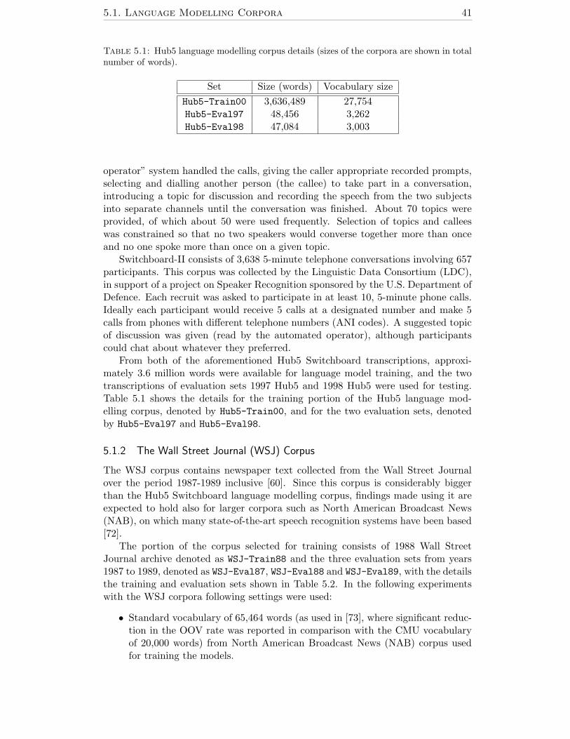
5.1. Language Modelling Corpora 41
Table 5.1: Hub5 language modelling corpus details (sizes of the corpora are shown in totalnumber of words).
Set Size (words) Vocabulary size
Hub5-Train00 3,636,489 27,754Hub5-Eval97 48,456 3,262Hub5-Eval98 47,084 3,003
operator” system handled the calls, giving the caller appropriate recorded prompts,selecting and dialling another person (the callee) to take part in a conversation,introducing a topic for discussion and recording the speech from the two subjectsinto separate channels until the conversation was finished. About 70 topics wereprovided, of which about 50 were used frequently. Selection of topics and calleeswas constrained so that no two speakers would converse together more than onceand no one spoke more than once on a given topic.
Switchboard-II consists of 3,638 5-minute telephone conversations involving 657participants. This corpus was collected by the Linguistic Data Consortium (LDC),in support of a project on Speaker Recognition sponsored by the U.S. Department ofDefence. Each recruit was asked to participate in at least 10, 5-minute phone calls.Ideally each participant would receive 5 calls at a designated number and make 5calls from phones with different telephone numbers (ANI codes). A suggested topicof discussion was given (read by the automated operator), although participantscould chat about whatever they preferred.
From both of the aforementioned Hub5 Switchboard transcriptions, approxi-mately 3.6 million words were available for language model training, and the twotranscriptions of evaluation sets 1997 Hub5 and 1998 Hub5 were used for testing.Table 5.1 shows the details for the training portion of the Hub5 language mod-elling corpus, denoted by Hub5-Train00, and for the two evaluation sets, denotedby Hub5-Eval97 and Hub5-Eval98.
5.1.2 The Wall Street Journal (WSJ) Corpus
The WSJ corpus contains newspaper text collected from the Wall Street Journalover the period 1987-1989 inclusive [60]. Since this corpus is considerably biggerthan the Hub5 Switchboard language modelling corpus, findings made using it areexpected to hold also for larger corpora such as North American Broadcast News(NAB), on which many state-of-the-art speech recognition systems have been based[72].
The portion of the corpus selected for training consists of 1988 Wall StreetJournal archive denoted as WSJ-Train88 and the three evaluation sets from years1987 to 1989, denoted as WSJ-Eval87, WSJ-Eval88 and WSJ-Eval89, with the detailsthe training and evaluation sets shown in Table 5.2. In the following experimentswith the WSJ corpora following settings were used:
• Standard vocabulary of 65,464 words (as used in [73], where significant reduc-tion in the OOV rate was reported in comparison with the CMU vocabularyof 20,000 words) from North American Broadcast News (NAB) corpus usedfor training the models.

5.2. Baseline Models 42
Table 5.2: WSJ language modelling corpus details (sizes of the corpora are shown in totalnumber of words).
Set Size (words) Vocabulary size
WSJ-Train88 17,057,940 107,065WSJ-Eval87 22,452 3,793WSJ-Eval88 21,947 4,092WSJ-Eval89 22,489 4,036
Table 5.3: Total number of words in the kept and held-out portions of the training datafor Hub5-Train00 and WSJ-Train88 together with the wordlist sizes.
Set Kept Set |KT | Held-out Set |HT | Vocabulary |V|
Hub5-Train00 3,527,238 109,251 27kWSJ-Train88 16,989,671 68,240 65k
• All the singleton events were discarded.
• All the evaluation sets were obtained from the WSJ language model develop-ment data for the corresponding year and constrained to have approximately20,000 words.
• Symbol marking the beginning of a sentence was not predicted during thelanguage model testing.
5.2 Baseline Models
The division of the training data T necessary for using the cross-validation, wasdone for both the 2000 Hub5 language modelling training data (Hub5-Train00) andthe 1988 WSJ training data (WSJ-Train88), with the sizes of the kept parts KT andthe held-out parts HT shown in Table 5.3 together with the corresponding wordlist sizes |V| used in the experiments. As can be seen from the table, the held-outportion of a larger WSJ training corpus is smaller than the held-out portion of theSwitchboard language model training corpus. There was no particular reason forsuch a division, with the only consideration being that the held-out set should besignificantly smaller than the kept set.
The baseline model for the Hub5 evaluation was chosen to be the trigram back-off model using the Good-Turing discounting with frequency of frequencies (FoF)discounting range of 8 and no event or context cutoffs. The baseline model forthe WSJ evaluations was chosen to be the trigram back-off model with FoF rangeof 8 and with the singleton events cutoffs applied to trigrams and bigrams. Bothback-off models were built on the whole training corpus T to ensure that back-offmodels and linear and log-linear interpolation models use the same overall amountof training data. Perplexities of the back-off models with respect to the evaluationsets described in previous section are shown in Table 5.4.

5.3. Linear Interpolation 43
Table 5.4: Perplexities of the baseline back-off models trained on 2000 Hub5 languagemodel training data and on 1988 WSJ training data, tested on the respective evaluationsets.
Model Test Set Perplexity
Hub5-Train00 Hub5-Eval97 98.2Hub5-Eval98 97.5
WSJ-Train88 WSJ-Eval87 165.2WSJ-Eval88 199.3WSJ-Eval89 198.0
100 101 102 103 104 105 106
100
150
200
250
300
Number of n−grams to fall into cluster
Perp
lexit
y
Hub5−Eval97 Hub5−Eval98
Figure 5.1: Influence of cluster size Nmin on the performance of linear interpolation ofmaximum likelihood estimates.
5.3 Linear Interpolation
In this section the experiments with trigram linear interpolation models carriedover Hub5 Switchboard and Wall Street Journal language modelling corpora aredescribed. The results are presented for two different cases, the first one concerningthe linear smoothing of the maximum likelihood estimates and the second one thelinear smoothing of Katz back-off models.
Maximum likelihood estimates
First, the optimal clustering scheme for linear interpolation of maximum likelihoodestimates, was selected by experimenting with different values of clustering con-straint Nmin defined in Sect.4.1.1, which essentially defines the bins for the interpo-lation weights. Influence of this parameter on the overall performance of the linearinterpolation model on two of the abovementioned data sets is shown in Figure 5.1.The worst result is obtained when no clustering is used at all, corresponding toNmin = 1, by keeping a separate interpolation weight for each n-gram history. In

5.3. Linear Interpolation 44
101 102 103 104 105 10693.6
93.8
94
94.2
94.4
94.6
94.8
95
95.2
95.4
Number of n−gram histories to fall into cluster (Nmin)
Perp
lexit
y
Hub5−Eval97Hub5−Eval98
Figure 5.2: Influence of cluster size Nmin on the performance of linear interpolation ofKatz back-off models.
this case there is never going to be enough data to accurately estimate such an enor-mous number of parameters and the resulting perplexities are high. The optimalperplexities, obtained on both test sets and found to correspond to Nmin = 104, areshown in Table 5.5, with perplexity on the Hub5-Eval97 test set equal to 99.3 andthe perplexity on the Hub5-Eval98 test set equal to 98.1, both slightly higher thanthe corresponding baseline back-off model perplexities.
Back-off estimates
According to the expectations, the linear interpolation of the back-off probabilityestimates should perform at least as well as the back-off model itself. In order tocheck this claim, recursive model consisting of linear combination of back-off scores,where the recursion is terminated by taking the back-off probability estimate of aunigram, defined similarly to (4.3) as
PLI(wi|wi−1i−n+1) = (1 − λ
wi−1i−n+1
)PBO(wi|wi−1i−n+1) +
λwi−1
i−n+1PLI(wi|w
i−1i−n+2) (5.1)
was built and tested. Each back-off estimate was obtained from the conventionalKatz smoothing model, introduced in Sect.3.2.11, with the basic Good-Turing dis-counting applied to small counts. Similarly to the maximum likelihood case dis-cussed above, the probability estimates were obtained from the kept part of thetraining set and the interpolation parameters were trained on the held-out set. Fig-ure 5.2 shows the results of the optimal clustering experiment conducted on the twoHub5 test sets. By comparing the performance of the conventional back-off modeltrained using the whole training corpus (both held-out and kept parts) with the lin-ear combination of back-off estimators presented above, the superiority of the latter
1The discounting frequency used was k = 8 and no context or event cut-offs were applied.

5.4. Log-Linear Interpolation 45
Table 5.5: Performance of the linear interpolation models (maximum likelihood and back-off estimates) with clustering constraint of Nmin = 104 and back-off language model on thetwo test sets from Hub5.
Models PerplexityHub5-Eval97 Hub5-Eval98
back-off 98.2 97.5linear interp. (ML) 99.3 98.1
linear interp. (back-off) 94.5 93.6
model is evident regardless of the clustering criteria. The optimal clustering param-eter Nmin, for which the biggest perplexity reduction was achieved, was yet againfound to be Nmin ≈ 104. The value of optimal clustering parameter depends on thesize of the training set and on the ratio δ between the held-out set and the kept setsizes. It may be expected that the value of the optimal parameter corresponding tothe different layout of the training data will be different.
The optimal perplexities of both best models, corresponding to clustering cri-terion of Nmin = 104, on two test sets are shown in Table 5.5. As can be seen,although the back-off model outperforms the linear interpolation of maximum like-lihood estimates on the both test sets, the differences in perplexities are small.Linear interpolation of back-off estimates, however, consistently outperforms theback-off model and the reduction of perplexity achieved over the baseline back-offmodel is 3.7% on the Hub5-Eval97 test corpus and 4% on Hub5-Eval98 test corpus.
5.4 Log-Linear Interpolation
In the following experiments, the probability estimates to be smoothed are takento be conventional Katz back-off estimates using Good-Turing discounting. Theexperiments were conducted on both Hub5 Switchboard and WSJ corpora.
5.4.1 Performance on Hub5 1997/1998 evaluation sets
Trigram log-linear interpolation model was built using the 2000 Hub5 language mod-elling data Hub5-Train00, which was divided into the kept and held-out portions,as described in Sect.5.2, where similarly to linear smoothing, kept part of the corpuswas used for obtaining the trigram, bigram and unigram Katz back-off probabilityestimates, and the held-out portion was used for optimising the log-linear smooth-ing weights. Powell multidimensional direct search [62] was used for the parameteroptimisation.
The influence of the clustering constraint Nmin on the performance of the modelon the two test sets against the baseline linear smoothing models (described in pre-vious section) is shown in Figure 5.3. As can be noted from the figure, the log-linearsmoothing is better behaved for the high values of clustering parameters Nmin withthe smaller rate of increase in perplexity than in the linear smoothing case. Forsmaller values of clustering parameters, however, linear smoothing performs in amore stable manner. Both linear and log-linear smoothing models outperform thebaseline back-off models by 3.5% to 4%, with the log-linear interpolation modelperforming slightly worse than its linear counterpart on the Hub5-Eval98 test set
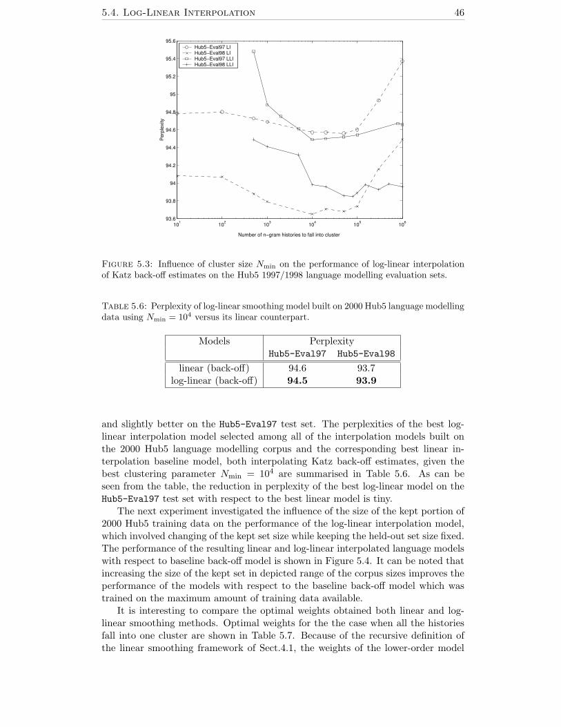
5.4. Log-Linear Interpolation 46
101 102 103 104 105 10693.6
93.8
94
94.2
94.4
94.6
94.8
95
95.2
95.4
95.6
Number of n−gram histories to fall into cluster
Perp
lexit
y
Hub5−Eval97 LI Hub5−Eval98 LI Hub5−Eval97 LLIHub5−Eval98 LLI
Figure 5.3: Influence of cluster size Nmin on the performance of log-linear interpolationof Katz back-off estimates on the Hub5 1997/1998 language modelling evaluation sets.
Table 5.6: Perplexity of log-linear smoothing model built on 2000 Hub5 language modellingdata using Nmin = 104 versus its linear counterpart.
Models PerplexityHub5-Eval97 Hub5-Eval98
linear (back-off) 94.6 93.7log-linear (back-off) 94.5 93.9
and slightly better on the Hub5-Eval97 test set. The perplexities of the best log-linear interpolation model selected among all of the interpolation models built onthe 2000 Hub5 language modelling corpus and the corresponding best linear in-terpolation baseline model, both interpolating Katz back-off estimates, given thebest clustering parameter Nmin = 104 are summarised in Table 5.6. As can beseen from the table, the reduction in perplexity of the best log-linear model on theHub5-Eval97 test set with respect to the best linear model is tiny.
The next experiment investigated the influence of the size of the kept portion of2000 Hub5 training data on the performance of the log-linear interpolation model,which involved changing of the kept set size while keeping the held-out set size fixed.The performance of the resulting linear and log-linear interpolated language modelswith respect to baseline back-off model is shown in Figure 5.4. It can be noted thatincreasing the size of the kept set in depicted range of the corpus sizes improves theperformance of the models with respect to the baseline back-off model which wastrained on the maximum amount of training data available.
It is interesting to compare the optimal weights obtained both linear and log-linear smoothing methods. Optimal weights for the the case when all the historiesfall into one cluster are shown in Table 5.7. Because of the recursive definition ofthe linear smoothing framework of Sect.4.1, the weights of the lower-order model

5.4. Log-Linear Interpolation 47
0.5 1 1.5 2 2.5 3 3.5 4 4.5x 10⁶
92
94
96
98
100
102
104
106
108
110
Kept set size (number of words)
Perp
lexit
y
Hub5−Eval97 LI Hub5−Eval97 LLIHub5−Eval97 BO
(a) Hub5-Eval97: Baseline back-off perplexity is 98.2
0.5 1 1.5 2 2.5 3 3.5 4 4.5x 10⁶
90
93
96
99
102
105
108
111
114
117
120
Kept set size (number of words)
Perp
lexit
y
Hub5−Eval98 LI Hub5−Eval98 LLIHub5−Eval98 BO
(b) Hub5-Eval98: Baseline back-off perplexity is 97.5
Figure 5.4: Influence of the size of the kept portion of 2000 Hub5 training set on theperformance of linearly and log-linearly smoothed Katz back-off estimates.

5.4. Log-Linear Interpolation 48
Table 5.7: Optimal linear and log-linear interpolation weights trained on 2000 Hub5language model training corpus with Nmin = 106, with the pair of interpolation weightscorresponding to bigram model, and the 3-tuple to the trigram model.
WeightsSmoothing bigram trigram
λbi0 λbi
1 λtri0 λtri
1 λtri2
linear 0.012123 0.987877 0.0017154 0.139786 0.858498log-linear −0.014994 0.967262 0.0023987 0.037057 0.896499
are reused in a higher-order model. In trigram case, for instance,
λtri2 = 1 − λtri
λtri1 = λtriλbi
1
λtri0 = λtri(1 − λbi
1 )
and, for bigrams
λbi1 = 1 − λbi
λbi0 = λbi ,
where the two weights λbi and λtri uniquely define the trigram linear interpolationmodel. In case of log-linear smoothing, unlike linear interpolation, there is no ap-parent relation between the weights, they do not necessarily sum to one and can benegative which can be explained by the specific way in which the log-linear frame-work was defined, in which all the five weights are essential for defining the model.However, by examining the table, it can be noted that the absolute value of all thelog-linear weights is less than one, and although they do not necessarily sum to one,they are not very different from the corresponding linear smoothing weights. Anadditional interesting observation that has been made during the experiments con-cerns the values of the log-linear weights and is summarised in Table 5.8, where thetotal number of optimal weights whose absolute value is bigger than one is shownagainst the total number of optimal weights calculated for each level of a trigramlog-linear model. An overall statistic for the Hub5 corpus shows that absolute val-ues of approximately 21% of the total number of weights calculated exhibited theproperty of being more than one. In particular, the upper bound on such absolutevalues was found to be approximately equal to 1.3.
5.4.2 Performance on 1987–1989 WSJ evaluation sets
For the experiments with the Wall Street Journal archives, the trigram log-linearinterpolation models were built using the 1988 WSJ archive WSJ-Train88, where theKatz back-off estimates to be smoothed were obtained from the kept portion of thetraining data, 65k vocabulary was used and event cutoffs were applied to singletonbigram and unigram distributions. Nelder–Mead multidimensional direct search wasused for optimising the smoothing weights. In order to compare the performanceof the log-linear smoothing on this corpus, the baseline linear interpolation modelsand Katz back-off models were built using the same settings.

5.4. Log-Linear Interpolation 49
Table 5.8: Total number of optimal log-linear smoothing weights calculated for each levelof all the log-linear trigram language models trained during the experiments against thetotal number of optimal weights whose absolute values exceeded unity for Hub5 1997/1998language model evaluation sets.
Model Level # λ # |λ| > 1
bigram 2008 456trigram 3669 726
overall 5677 1182
Table 5.9: Optimal linear and log-linear interpolation weights trained on 1988 WSJ lan-guage model training corpus with Nmin = 107, with the pair of interpolation weights corre-sponding to bigram model, and the 3-tuple to the trigram model.
WeightsSmoothing bigram trigram
λbi0 λbi
1 λtri0 λtri
1 λtri2
linear 0.0066299 0.993370 0.0003469 0.05198306 0.94767log-linear 0.0017205 0.965193 0.0225268 −0.0262599 0.94396
Optimal weights obtained for the case where all the histories fall into one bin,corresponding to Nmin = 107, for both linear and non-linear smoothing are shownin Table 5.9. Similar to a Hub5 case, the absolute values of the vast majority of theweights obtained were less than 1.
Figure 5.5 displays the performance of the trigram log-linear model on thethree evaluation sets from the WSJ corpus. The performance of the correspondingbaseline linear interpolation models is displayed on the same plot for convenience.Performance of the log-linear model, as compared to the baseline Katz back-off andlinear interpolation, on the three test sets is summarised in Table 5.10. As canbe seen, log-linear interpolation compares favourably with the baseline techniques,with the perplexity reduction of 2.3% on the WSJ-Eval87 test set, 2.5% on theWSJ-Eval88 test set and 3.2% on the WSJ-Eval89 test set with respect to the Katzback-off baseline model. Moreover, log-linear interpolation outperforms linear inter-polation, with the reduction in perplexity of 2% on the WSJ-Eval89 test set, 2.1%
Table 5.10: Performance of the log-linear smoothing model built on 1988 WSJ languagemodelling data using versus its back-off and linear counterparts (best models, in terms ofthe clustering criterion) were selected).
Models PerplexityWSJ-Eval87 WSJ-Eval88 WSJ-Eval89
back-off 165.2 199.3 198.0linear (back-off) 164.6 198.5 196.8
log-linear (back-off) 161.4 194.4 191.7

5.4. Log-Linear Interpolation 50
104 105 106 107161.2
161.4
161.6
161.8
162
Perp
lexit
y (L
LI)
WSJ−Eval87 LLI
104 105 106 107164.5
164.6
164.7
164.8
164.9
Number of histories to fall into a bin
Perp
lexit
y (L
I)
WSJ−Eval87 LI
(a) WSJ-Eval87: Baseline back-off perplexity is 165.2
104 105 106 107194
194.2
194.4
194.6
194.8
195
Perp
lexit
y (L
LI)
WSJ−Eval88 LLI
104 105 106 107198.5
198.6
198.7
198.8
198.9
199
Number of histories to fall into a binPe
rple
xity
(LI)
WSJ−Eval88 LI
(b) WSJ-Eval88: Baseline back-off perplexity is 199.3
104 105 106 107191.65
191.7
191.75
191.8
191.85
191.9
191.95
192
Perp
lexit
y (L
LI)
WSJ−Eval89 LLI
104 105 106 107196.7
196.8
196.9
197
197.1
197.2
197.3
197.4
Number of histories to fall into a bin
Perp
lexit
y (L
I)
WSJ−Eval89 LI
(c) WSJ-Eval89: Baseline back-off perplexity is 198.0
Figure 5.5: Performance of trigram log-linear and linear interpolation models on1987/88/89 WSJ evaluation sets.
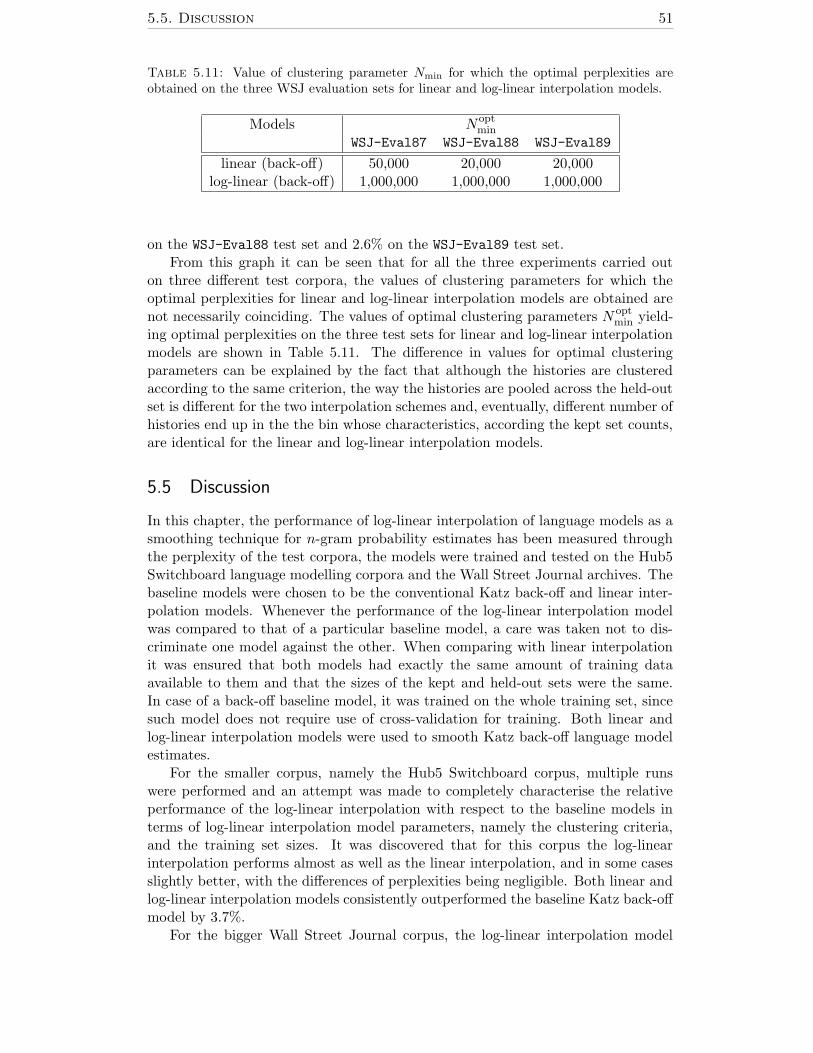
5.5. Discussion 51
Table 5.11: Value of clustering parameter Nmin for which the optimal perplexities areobtained on the three WSJ evaluation sets for linear and log-linear interpolation models.
Models Noptmin
WSJ-Eval87 WSJ-Eval88 WSJ-Eval89
linear (back-off) 50,000 20,000 20,000log-linear (back-off) 1,000,000 1,000,000 1,000,000
on the WSJ-Eval88 test set and 2.6% on the WSJ-Eval89 test set.From this graph it can be seen that for all the three experiments carried out
on three different test corpora, the values of clustering parameters for which theoptimal perplexities for linear and log-linear interpolation models are obtained arenot necessarily coinciding. The values of optimal clustering parameters N opt
min yield-ing optimal perplexities on the three test sets for linear and log-linear interpolationmodels are shown in Table 5.11. The difference in values for optimal clusteringparameters can be explained by the fact that although the histories are clusteredaccording to the same criterion, the way the histories are pooled across the held-outset is different for the two interpolation schemes and, eventually, different number ofhistories end up in the the bin whose characteristics, according the kept set counts,are identical for the linear and log-linear interpolation models.
5.5 Discussion
In this chapter, the performance of log-linear interpolation of language models as asmoothing technique for n-gram probability estimates has been measured throughthe perplexity of the test corpora, the models were trained and tested on the Hub5Switchboard language modelling corpora and the Wall Street Journal archives. Thebaseline models were chosen to be the conventional Katz back-off and linear inter-polation models. Whenever the performance of the log-linear interpolation modelwas compared to that of a particular baseline model, a care was taken not to dis-criminate one model against the other. When comparing with linear interpolationit was ensured that both models had exactly the same amount of training dataavailable to them and that the sizes of the kept and held-out sets were the same.In case of a back-off baseline model, it was trained on the whole training set, sincesuch model does not require use of cross-validation for training. Both linear andlog-linear interpolation models were used to smooth Katz back-off language modelestimates.
For the smaller corpus, namely the Hub5 Switchboard corpus, multiple runswere performed and an attempt was made to completely characterise the relativeperformance of the log-linear interpolation with respect to the baseline models interms of log-linear interpolation model parameters, namely the clustering criteria,and the training set sizes. It was discovered that for this corpus the log-linearinterpolation performs almost as well as the linear interpolation, and in some casesslightly better, with the differences of perplexities being negligible. Both linear andlog-linear interpolation models consistently outperformed the baseline Katz back-offmodel by 3.7%.
For the bigger Wall Street Journal corpus, the log-linear interpolation model

5.5. Discussion 52
outperformed the linear interpolation by 2% to 2.6% and the back-off languagemodel by 2.3% to 3.2% in terms of perplexity calculated over the three evaluationsets.
According to these findings it is possible to assume that log-linear smoothingof n-gram language models performs as well as linear interpolation on the smallcorpora and outperforms it on the bigger corpora, with both interpolation modelsachieving performance which is constistently superior to that of the unsmoothedback-off language model.
While an attempt has been made to systematically explore the log-linear smooth-ing for n-grams, there remain many directions that need to be explored, for example,it is interesting to see how the division of the training data into the kept and held-outsets (i.e. the ratio between the held-out and kept set sizes) affects the performanceof log-linear language model. When the size of the held-out set is too small, thedeterioration of the performance can be expected due to the fact that there is notenough data to estimate the interpolation weights, whereas if the kept set size istoo small, the deterioration in the performance can be explained by the insufficientamount of data for obtaining the probability estimates to be smoothed.

CHAPTER 6
Summary and Conclusion
In this work a novel smoothing technique for n-gram language modelling, namelythe log-linear interpolation was investigated. Log-linear interpolation of an n-gramlanguage models is a technique which allows to form an exponential combination ofprobability estimates obtained for n-grams of different specificity trained on sometext corpus. The resulting combination is guaranteed to perform no worse than theprobability estimates comprising the model provided that these n-gram probabilityestimates are reliable enough, i.e. some form of discounting was used to obtain themin order to ensure that the probabilities are nonzero. Maximum likelihood estimatesdo not satisfy this condition and therefore are not considered in this work.
Log-linear interpolation was introduced by Klakow [39] who used it for combiningdifferent language models. This technique, interpolating the conventional n-gramsand another type of language models called distance n-grams was successfully ap-plied by Beyerlein et al. [5] to the broadcast news transcription task. Unlike thepublications mentioned above, which essentially propose a general purpose methodfor combining the arbitrary language models, the aim of this work was to investi-gate the applicability of the technique to the special case of smoothing of n-gramprobability estimates, and to attempt a rigorous derivation of theoretical frameworkwithin which the log-linear interpolation could be placed as a possible smoothingmethod. As a result, the framework for obtaining the log-linear interpolation proba-bility estimates, including the techniques for parameter optimisation and clustering,was proposed.
In consequent experiments carried over the two popular language modelling cor-pora, the log-linear interpolation has shown to perform as well as linear interpolationwhen produced on a small corpus and outperform the linear interpolation on a bigcorpus, with both models outperforming the baseline back-off language model.
The log-linear interpolation of language models, as it has been shown in thiswork, seems to be a promising technique which can be successfully employed in thetasks of smoothing the language model probability estimates.
53

Bibliography
[1] L. R. Bahl, P. F. Brown, P. V. de Souza, and R. L. Mercer. A tree-based language model for natural language speech recognition. IEEE Transac-
tions on Acoustics, Speech, and Signal Processing, ASSP-37(7):1001–1008, July1989.
[2] L. R. Bahl, P. F. Brown, P. V. de Souza, R. L. Mercer, and D. Na-
hamoo. A fast algorithm for deleted interpolation. In Proceedings of the 2nd
European Conference on Speech Communication and Technology, volume 3,pages 1209–1212, Genova, September 1991.
[3] L. R. Bahl, F. Jelinek, and R. L. Mercer. A maximum likelihood ap-proach to continuous speech recognition. In A. Waibel and K. Lee, editors,Readings in Speech Recognition, chapter 6, pages 308–319. Morgan Kaufmann,San Mateo, CA, 1990. Reprinted from ’83 IEEE Transactions on Pattern Anal-
ysis and Machine Intelligence.
[4] A. L. Berger, S. A. Della Pietra, and V. J. Della Pietra. A maximumentropy approach to natural language processing. Computational Linguistics,22(1):39–71, March 1996.
[5] P. Beyerlein, X. L. Aubert, R. Haeb-Umbach, M. Harris, D. Klakow,
A. Wendemuth, S. Molau, M. Pitz, and A. Sixtus. The Philips/RWTHsystem for transcription of broadcast news. In Proceedings of the 6th European
Conference on Speech Communication and Technology, volume 2, pages 647–650, Budapest, September 1999.
[6] E. Black, F. Jelinek, J. Lafferty, R. L. Mercer, and S. Roukos.Decision tree models applied to the labelling of texts with parts-of-speech. In’92 DARPA Speech and Natural Language Workshop, pages 117–121, 1992.
[7] G. E. P. Box and G. C. Tao. Bayesian Inference in Statistical Analysis.Addison-Wesley, Reading, MA, 1973. Section 1.3.
[8] T. Briscoe and J. Carrol. Generalized probabilistic LR parsing of naturallanguage (corpora) with unification-based grammars. Computational Linguis-
tics, 19(1):25–59, 1993.
[9] P. F. Brown, V. J. Della Pietra, P. de Souza, J. C. Lai, and R. L.
Mercer. Class-based n-gram models of natural language. Computational
Linguistics, 18(4):467–479, 1992.
[10] P. F. Brown, V. J. Della Pietra, R. L. Mercer, S. A. Della Pietra,
and J. C. Lai. An estimate of an upper bound for the entropy of English.Computational Linguistics, 18(1):31–40, March 1992.
54

BIBLIOGRAPHY 55
[11] E. Charniak. Statistical Language Learning. Language, speech, and commu-nication. MIT Press, Cambridge, MA; London, 1993.
[12] C. Chelba and F. Jelinek. Exploiting syntactic structure for languagemodeling. In Proceedings of Association for Computational Linguistics, volumeACL-36, Montreal, 1998.
[13] S. F. Chen and J. Goodman. An empirical study of smoothing techniquesfor language modeling. In Proceedings of Association for Computational Lin-
guistics, volume ACL-34, pages 310–318, Santa Cruz, CA, June 1996.
[14] S. F. Chen and J. Goodman. An empirical study of smoothing techniquesfor language modeling. Technical Report TR-10-98, Computer Science Group,Harvard University, August 1998.
[15] S. F. Chen and J. Goodman. An empirical study of smoothing techniques forlanguage modeling. Computer Speech and Language, 13(4):359–394, October1999.
[16] S. F. Chen, K. Seymore, and R. Rosenfeld. Topic adaptation for languagemodeling using unnormalized exponential models. In Proceedings of IEEE In-
ternational Conference on Acoustics, Speech and Signal Processing, volume 2,pages 681–684, Seattle, Washington, May 1998.
[17] K. W. Church and W. A. Gale. A comparison of the enhanced Good-Turing and deleted estimation methods for estimating probabilities of Englishbigrams. Computer Speech and Language, 5(1):19–54, January 1991.
[18] K. W. Church and P. Hanks. Word association norms, mutual informationand lexicography. In Proceedings of Association for Computational Linguistics,volume ACL-27, pages 76–83, 1989.
[19] T. M. Cover and J. A. Thomas. Elements of Information Theory. WileySeries in Telecommunications. John Wiley & Sons, 1991.
[20] R. O. Duda and P. E. Hart. Pattern Classification and Scene Analysis.John Wiley & Sons, New York, 1973.
[21] W. N. Francis and H. Kucera. Frequency Analysis of English Usage: Lex-
icon and Grammar. Houghton-Mifflin, Boston, 1982.
[22] W. A. Gale and K. W. Church. Estimation procedures for language con-text: poor estimates are worse than none. In COMPSTAT, Proceedings in Com-
putational Statistics, pages 69–74, Dubrovnik, Yugoslavia, September 1990.
[23] W. A. Gale and G. Sampson. Good-Turing frequency estimation withouttears. Journal of Quantitative Linguistics, 2:217–237, 1995.
[24] J. Gao and X. Chen. Probabilistic word classification based on a context-sensitive binary tree method. Computer Speech and Language, 11(4):307–320,October 1997.
[25] M. Generet, H. Ney, and F. Wessel. Extensions of absolute discount-ing for language modeling. In Proceedings of the 4th European Conference on
Speech Communication and Technology, volume 2, pages 1245–1248, Madrid,September 1995.

BIBLIOGRAPHY 56
[26] J. J. Godfrey, E. C. Holliman, and J. McDaniel. SWITCHBOARD:Telephone speech corpus for research and development. In Proceedings of IEEE
International Conference on Acoustics, Speech and Signal Processing, volume 1,pages 517–520, San Francisco, March 1992.
[27] I. J. Good. The population frequencies of species and the estimation of pop-ulation parameters. Biometrika, 40(3/4):237–264, December 1953.
[28] J. Goodman. Putting it all together: Language model combination. In Pro-
ceedings of IEEE International Conference on Acoustics, Speech and Signal
Processing, volume 3, pages 1647–1650, Istanbul, June 2000.
[29] M. Jardino. A class bigram model for very large corpus. In Proceedings
of International Conference on Spoken Language Processing, volume 2, pages867–870, Yokohama, September 1994.
[30] H. Jeffreys. Theory of Probability. Oxford Science Publications. ClarendonPress, Oxford, 3rd edition, 1961.
[31] F. Jelinek. Markov source modelling of text generation. In J. K. Skwirzynski,editor, The Impact of Processing Techniques on Communication. Martinus-Nijhoff Publishers, Dordrecht, 1985.
[32] F. Jelinek. Self-organised language modeling for speech recognition. InA. Waibel and K. Lee, editors, Readings in Speech Recognition, chapter 8,pages 450–503. Morgan Kaufmann, San Mateo, CA, 1990.
[33] F. Jelinek. Statistical Methods for Speech Recognition. Language, speech andcommunication. MIT Press, Cambridge, MA; London, March 1997.
[34] F. Jelinek and R. L. Mercer. Interpolated estimation of Markov sourceparameters from sparse data. In Proceedings of the Workshop on Pattern Recog-
nition in Practice. North-Holland, Amsterdam, May 1980.
[35] F. Jelinek and R. L. Mercer. Probability distribution estimation fromsparse data. IBM Technical Disclosure Bulletin, (28):2591–2594, 1985.
[36] I. Kanter and D. A. Kessler. Markov processes: Linguistics and Zipf’slaw. Physical Review Letters, 74(22):4559–4562, May 1995.
[37] S. Katz. Estimation of probabilities from sparse data for the language modelcomponent of a speech recognizer. IEEE Transactions on Acoustics, Speech,
and Signal Processing, ASSP-35(3):400–401, March 1987.
[38] C. T. Kelley. Detection and remediation of stagnation in the Nelder–MeadAlgorithm using a sufficient decrease condition. Society for Industrial and Ap-
plied Mathematics Journal on Optimization, 10(1):43–55, 1999.
[39] D. Klakow. Log-linear interpolation of language models. In Proceedings of
5th International Conference on Spoken Language Processing, volume 5, pages1695–1699, Sydney, December 1998.
[40] R. Kneser and H. Ney. Improved backing-off for m-gram language mod-eling. In Proceedings of IEEE International Conference on Acoustics, Speech
and Signal Processing, volume 1, pages 181–184, Detroit, May 1995.

BIBLIOGRAPHY 57
[41] H. Kucera and W. N. Francis. Computational Analysis of Present-Day
American English. Brown University Press, Providence, RI, 1967.
[42] J. C. Lagarias, J. A. Reeds, M. H. Wright, and P. E. Wright. Con-vergence properties of the Nelder–Mead Simplex method in low dimensions.Society for Industrial and Applied Mathematics Journal on Optimization, 9(1):112–147, 1998.
[43] P. S. Laplace. Philosophical Essay on Probabilities, volume 13 of Sources in
the history of mathematics and physical sciences. Springer-Verlag, New York,1995. Translated from the 5th French edition of 1825.
[44] E. L. Lehmann. Theory of Point Estimation. Probability and mathematicalstatistics. John Wiley & Sons, New York, 1983.
[45] W. Li. Random texts exhibit Zipf’s-law-like word frequency distribution. IEEE
Transactions on Information Theory, 38(6):1842–1845, 1992.
[46] W. Li. Comments on Zipf’s law and the structures and evolution of naturallanguages. Complexity, 3(5):9–10, 1998. Letters to the editor.
[47] D. Magerman. Natural Language Parsing as Statistical Pattern Recognition.Ph.D. dissertation, Stanford University, February 1994. Section 3.4.2.
[48] B. B. Mandelbrot. The Fractal Geometry of Nature. W. H. Freeman, NewYork, 1983.
[49] C. D. Manning and H. Schutze. Foundations of Statistical Natural Lan-
guage Processing. Language, speech, and communication. MIT Press, Cam-bridge, MA; London, August 1999. Section 1.4.3.
[50] S. C. Martin, C. Hamacher, J. Liermann, F. Wessel, and H. Ney.Assessment of smoothing methods and complex stochastic language modeling.In Proceedings of the 6th European Conference on Speech Communication and
Technology, volume 5, pages 1939–1942, Budapest, September 1999.
[51] S. C. Martin, H. Ney, and J. Zaplo. Smoothing methods in maximumentropy language modeling. In Proceedings of IEEE International Conference
on Acoustics, Speech and Signal Processing, volume I, pages 545–548, Phoenix,March 1999.
[52] D. D. McDonald. Internal and external evidence in the identification andsemantic categorization of proper names. In B. Boguraev and J. Pustejovsky,editors, Corpus Processing for Lexical Acquisition, Language, speech, and com-munication, pages 21–39. MIT Press, Cambridge, MA; London, 1995.
[53] K. I. M. McKinnon. Convergence of the Nelder–Mead Simplex method to anonstationary point. Society for Industrial and Applied Mathematics Journal
on Optimization, 9(1):148–158, 1998.
[54] A. Nadas. On Turing’s formula for word probabilities. IEEE Transactions
on Acoustics, Speech, and Signal Processing, ASSP-33(6):1414–1416, December1985.

BIBLIOGRAPHY 58
[55] H. Ney and U. Essen. On smoothing techniques for bigram-based natu-ral language modelling. In Proceedings of IEEE International Conference on
Acoustics, Speech and Signal Processing, volume 2, pages 825–828, Toronto,May 1991.
[56] H. Ney and U. Essen. Estimating ‘small’ probabilities by leaving-one-out.In Proceedings of the 3rd European Conference on Speech Communication and
Technology, volume 3, pages 2239–2242, Berlin, September 1993.
[57] H. Ney, U. Essen, and R. Kneser. On structuring probabilistic dependen-cies in stochastic language modeling. Computer Speech and Language, 8(1):1–28, January 1994.
[58] H. Ney, S. Martin, and F. Wessel. Statistical language modeling usingleaving-one-out. In S. Young and G. Bloothooft, editors, Corpus-Based Methods
in Language and Speech Processing, chapter 6, pages 174–207. Kluwer AcademicPublishers, Dordrecht, 1997.
[59] T. Niesler. Category-based statistical language models. Ph.D. dissertation,Cambridge University, June 1997.
[60] D. B. Paul and J. M. Baker. The design for the Wall Street Journal-basedCSR corpus. In Proceedings of International Conference on Spoken Language
Processing, pages 899–902, 1992.
[61] L. C. Bauman Peto. A Comparison of Two Smoothing Methods for Word
Bigram Models. M.Sc. dissertation, Graduate Department of Computer Science,University of Toronto, October 1994.
[62] W. H. Press, B. P. Flannery, S. A. Teukolsky, and W. T. Vet-
terling. Numerical Recipes: The Art of Scientific Computing. CambridgeUniversity Press, 1986.
[63] E. S. Ristad. A natural law of succession. Research Report CS-TR-495-95,Department of Computer Science, Princeton University, July 1995.
[64] R. Rosenfeld. Adaptive Statistical Language Modeling: A Maximum En-
tropy Approach. Ph.D. dissertation, Carnegie Mellon University, April 1994.Published as Research Report CMU-CS-94-138. Appendix B.
[65] C. Samuelsson. Relating Turing’s formula and Zipf’s law. Research ReportCLAUS-78, Computational Linguistics Department, Universitat des Saarlan-des, Saarbrucken, June 1996.
[66] C. E. Shannon. Prediction and entropy of printed English. The Bell System
Technical Journal, 30:50–64, January 1951.
[67] H. S. Sichel. On a distribution law for word frequencies. Journal of the
American Statistical Association, 70(351):542–547, September 1975.
[68] Z. K. Silagadze. Citations and the Zipf-Mandelbrot’s law. Complex Systems,11(6), 2000.
[69] R. F. Simmons and Y. Yu. The acquisition and use of context-dependentgrammars for English. Computational Linguistics, 18(4):391–418, December1992.

BIBLIOGRAPHY 59
[70] A. A. Tsonis, C. Schultz, and P. A. Tsonis. Zipf’s law and the structureand evolution of languages. Complexity, 2(5):12–13, 1997.
[71] F. Wessel and A. Baader. Robust dialogue-state dependent language mod-eling using leaving-one-out. In Proceedings of IEEE International Conference
on Acoustics, Speech and Signal Processing, volume II, pages 741–744, Phoenix,March 1999.
[72] P. C. Woodland, M. J. F. Gales, D. Pye, and V. Valtchev. The HTKlarge vocabulary recognition system for the 1995 ARPA H3 task. In Proceedings
of the ARPA Speech Recognition Workshop, New York, 1996. Harriman House.
[73] P. C. Woodland, C. J. Leggetter, J. J. Odell, V. Valtchev, and
S. J. Young. The 1994 HTK large vocabulary speech recognition system. InProceedings of IEEE International Conference on Acoustics, Speech and Signal
Processing, volume 1, pages 73–76, Detroit, May 1995.
[74] G. K. Zipf. Human Behaviour and the Principle of Least Effort. Addison-Wesley, Reading, MA, 1949.
[75] G. K. Zipf. The Psycho-Biology of Language: An Introduction to Dynamic
Philology. MIT Press, Cambridge, MA, 1968. Reprint of Houghton-Mifflinedition of 1935.