locument resume ed 374 138 tm 022 013 author … · identifiers biodata; indicators; *proportional...
TRANSCRIPT

LOCUMENT RESUME
ED 374 138 TM 022 013
AUTHOR McCloy, Rodney A.; And OthersTITLE Prediction of First-Term Military Attrition Using
Pre-Enlistment Predictors.SPONS AGENCY Army Research Inst. for the Behavioral and Social
Sciences, Alexandria, Va.PUB D:TE Aug 93CONTRACT MDA-903-89-C-0202NOTE 66p.; Paper presented at the Annual Meeting of the
American Psychological Association (101st, Toronto,Oi.cario, Canada, August 1993).
PUB TYPE Reports Research/Technical (143)Speeches /Conference Papers (150)
EDRS PRICE MF01/PC03 Plus Postage.DESCRIPTORS Career Choice; Cost Effectiveness; *Educational'
Attainment; High School Graduates; *Labor Turnover;*Military Personnel; Military Training; *OccupationalTests; *Personality Traits; *Prediction; PredictorVariables; Regression (Statistics)
IDENTIFIERS Biodata; Indicators; *Proportional Hazards Models
ABSTRACTSoldiers who exit the Army before the end of their
first term of service represent lost investments in terms of bothdirect costs (e.g., training costs) and indirect costs (e.g., forceinstability). The Army would benefit from pre-enlistment informationthat could identify those individuals most likely to Complete theirfirst term. This paper examines the relationship between first-termmilitary attrition, information currently available to the Army(e.g., high school diploma graduate status), and three non-cognitivemeasures developed and administered during the Army's ProjectA/Building the Career Force research program (Campbell and Zook,1990a; Campbell and Zook, 1992). Proportional hazards regressionmodels were estimated for 4 job groups (roughly 49,000 first-termsoldiers) using hierarchical and empirical "best-model" approaches. Abattery of predictors is proposed for predicting attrition in allfour job groups. The Army can improve prediction of attrition bygathering biodata and temperament information prior to enlistment andby better using information they currently possess. Nine figures and16 tables present study information. (Contains 26 references.)(Author/SLD)
****************.*******************************************************
Reproductions supplied by EDRS are the best that can be madefrom the original document.
**********************************************************************

U.S. OEPAIRTNIENT Of EDUCATIOROffice ot Educattonal Research and Improvement
ED ATIONAL RESOURCES INFORMATIONCENTER (ERIC)
his document has been reproduced a3received from IN person or organizationoriginating itPAM' changes have Wan made to improvereproduction Quality
Points of view Or opinions stated in this docu-mnt do not neCessarily represent officialOEM outdoor+ or porrty
First-Term Att.ition
"PERMISSION TO REPRODUCE THISMATERIAL HAS BEEN GRANTED BY
akowEy /9.P eetoy
TO THE EDUCATIONAL RESOURCESINFORMATION CENTER (ERIC)."
Prediction of First-Term Military Attrition
Using Pre-Enlistment Predictors
Rodney A. McCloy, Ani S. DiFazio
Human Resources Research Organization
Gary W. Carter
U. S. Department of Labor
Paper presented as part of the symposium, "Predictionof Turnover in a Longitudinal Sample Using EventHistory Analysis" at the 101st Annual Convention ofthe American Psychological Association, Toronto,Ontario, Canada, August 22, 1993.
This research was funded by the U.S. Army Research .Institute for the Behavioral and SocialSciences, Contract No. MDA903-89-C-0202. All statements expressed in this paper are thoseof the authors and do not necessarily reflect the official opinions or policies of the U.S.Army Research Institute or the Department of the Army.
2BEST COPY AVAILABLE
1

First-Term Attrition
2
Abstract
Soldiers who exit the Army before the end of their first
term of service represent lost investments in terms-of both direct
costs (e.g., training costs) and indirect costs (force
instability). The Army would benefit from pre-enlistment
information that could identify those individuals most likely to
complete their first term. This paper examines the relationship
between first-term military attrition, information currently
available to the Army (e.g., high school diploma graduate status),
and three non-cognitive measures developed and administered during
the Army's Project A/Building the Career Force research program
(Campbell & Zook, 1990a; Campbell & Zook, 1992). Proportional
hazards regression models were estimated for four job groups using
hierarchical and empirical "best-model" approaches. A battery of
predictors is proposed for predicting attrition in all four job
groups.
3

First-Term Attrition
3.
Prediction of First-Term Military Attrition
Using Pre-Enlistment Predictors
Soldiers who fail to complete their first term of military
service are costly to the Services. Klein, Hawes-Dawson, and
Martin (1991) conservatively estimated the cost of first-term
attrition to be 200 million dollars (in 1989 dollars). Such
direct costs include lost investments such as training costs,
recruiting costs, and compensation costs in the form of salary
. during. enlistment and subsequent unemployment costs (e.g.,
Laurence, 1993; McCloy et al., 1992). Laurence further noted that
attrition also results in significant indirect costs, both to the
military (in the form of lowered morale and force instability) and
to the individual (in the form of possibly reduced future
employment opportunities and earning potential). As'a result,
significant benefits can accrue from better understanding the
precursors of attrition and using this information to select those
recruits who are less likely to exit the military prematurely.
The Services currently use high-school diploma graduate
status as an indicator of a recruit's chances of completing his or
her first term, a practice spurred by an initial Air Force
technical report (Flyer, 1959) and since justified by years of
supporting evidence. As Laurence (1993) stated, the Flyer study
"was only the first in a very long line of research to conclude
that high school graduates have lower attrition rates [than non-
diploma graduates] . . . [and] similar findings have been echoed
4

First-Term Attrition
4
in countless reports over the past 30 plus years" (p. 5).
In contrast, very little relationship has been found between
measures of cognitive ability and attrition. High-school
graduates scoring in the lowest part of the distribution on the
Armed Forces Qualification Test (AFQT) have lower rates of
attrition than non-graduates in the uppermost part of the
distribution. Laurence (1993) suggested that the relationship
between first-term attrition and diploma status might be due to
differences between the two groups on various non-cognitive
characteristics. These characteristics, in turn, are typically
assessed with instruments such as temperament, interest, or
biodata inventories.
Indeed, although high-school diploma status is the single
best predictor of first-term attrition, biodata instruments have
demonstrated incremental validity (e.g., Steinhaus, 1988; Trent,
1993; White, Nord, Mael, & Young, 1993). Further, research from
the Army's Project A (Campbell & Zook, 1990a) and the follow-on
Career Force project (Campbell & Zook, 1992) has demonstrated the
validity of non-cognitive measures for predicting the volitional,
or "will-do," dimensions of Army job performance (e.g., effort,
physical fitness and military bearing, personal discipline) --
dimensions that may impact attrition.
Building on this research, the goal of the present study was
to determine the relationship between first-term Army attrition
and various pre-enlistment predirt.ors, including scores on three

First-Term Attrition
5
non-cognitive predictor instruments developed as part of the
Project A/Building the Career Force research program -- a large-
scale, multi-year research program intended to develop an improved
selection and classification system for initial assignment of
persons to U. S. Army occupations, or Military Occupational
Specialties (MOS). The three inventories include a biodata and
temperament measure, an interest measure, and a measure of job
outcome preferences or values. The primary research question was
which, if any, of the experimental non-cognitive measures would
provide incremental prediction to the information already
available to the Army: (1) test scores from the military
enlistment test, the Armed Services Vocational Aptitude Battery
(ASVAB), and (2) high school diploma graduate status.
Event History Analysis and the Proportional Hazards Model
The relationship between first-term attrition and the pre-
enlistment predictors was addressed using proportional hazards
modelling (Cox, 1972), a form of event history analysis (cf.
Allison, 1984). Event history analysis allows a researcher to
model whether or not an event occurs, and if so, when it occurs.
In the present research, the event is attrition from the Army
during the first term of enlistment. Specifically, a proportional
hazards model allows one to determine the relationship between one
or more predictor variables and the rate at which events occur
over time:
6

First-Term Attrition
6
in [h(t) ] = in [ho(t) + (31L (1)
where In is the natural logarithm, h(t) is the hazard rate, ho(t)
is a baseline hazard rate that can take any form (i.e., it is non-
parametric), p is a vector of regression coefficients with a
specific functional form (i.e., it is parametric), and X is a
vector of predictor variables.
. Working with event data presents several analytic
difficulties that more conventional analytic methods do not handle
well, including non-normal distributions, time-varying independent
variables, and subjects who do not experience the event of
interest during the observation period -- observations that are
"censored" (cf. Allison, 1984; Lawless, 1982; Singer & Willett,
1991). Event history analysis does not rely upon normality
assumptions, easily accommodates time-varying independent
variables', and makes maximal use of the data provided by
censored observations. Thus, event history analysis provides a
proper analytic method for event data and is therefore ideal for
the analysis of first-term military attrition. In particular, the
proportional hazards model is very flexible in that it does not
require the researcher to specify a particular distribution for
the events across time. Consequently, the proportional hazards
'Although the proportional hazards model discussed here easilyincorporates time-varying independent variables, most event models that assumethe event times to follow a specific distribution (i.e., parametric models) donot. Parametric models involving such variables can be estimated (e.g., Flinn& Heckman, 1982) but only with great difficulty.

First-Term Attrition
7
model was chosen to examine the relationship between attrition and'
several pre-enlistment predictors. (See McCloy, 1993, for a more
detailed discussion of the fundamental properties of event history
models.)
Method
Subjects
The subjects were the roughly 49,000 first-term soldiers
from the Project A/Career Force Longitudinal Validation (LV)
sample (Campbell & Zook, 1992). These soldiers were administered
a four-hour Experimental Predictor Battery (Campbell & Zook,
1990a) within 2 days of their entry into the Army. The data were
collected over a 14-month period (August 20, 1986 through November
30, 1987) at eight Reception Battalions. The soldiers represented
the 21 MOS listed in Table 1.
- - Insert Table 1 About Here - - -
Data checks for out-of-range values (e.g., impossible or
incompatible entry and exit dates) reduced the sample to 48,308.
Listwise deletion was performed on the pre-enlistment measures
used to model attrition, yielding a final sample size of 31,032
soldiers.
Job groups. Rather than running analyses by MOS, job groups
were formed by splitting the 21 MOS listed in Table 1 into two
groups: Combat (MOS 11B, 13B, 16S, 19E, and 19K) and Non-Combat
(all others). These two groups were further separated by
enlistment terms.
3

First-Term Attrition
8
In many applications of event history analysis, the
endpoints and length of the observation period are arbitrary,
being driven by convenience or a desire to observe a certain
number of events. First-term attrition, however, has clear
starting and ending points, beginning when the soldier enters the
military and ending at the conclusion of the enlistment term
agreed upon on the enlistment contract. Army enlistment terms
typically range from two to six years, with three-year and four-
year terms being the most common. The present study contains only
those soldiers who agreed to three-year and four-year terms.
Because the two terms of enlistment provide meaningful
observation periods of different duration, the two MOS groups were
further split by term, yielding four analysis groups: soldiers in
Combat and Non-Combat MOS with 3-year and 4-year enlistment terms
(C3, C4, NC3, and NC4, respectively). Note that all six Combat
MOS appear in both enlistment term groups (C3 and C4) because they
contain many soldiers with three-year terms and many soldiers with
four-year enlistment terms. Similarly, three of the Ndn-Combat
MOS (76Y, 94B, and 95B) appear in both Non-Combat enlistment term
groups (NC3 and NC4). The MOS within each of the four job groups,
the sample sizes for each, the number and percentage who
experienced attrition, and the number and percentage who were
censored observations are given in Tables 2 through 5.
- - - - Insert Tables 2-5 About Here - - - -
9

First-Term Attrition
9
Measures
Attrition. For this research, attrition is defined as a
premature separation from first term service for reasons that
might be viewed negatively from the military perspective. There
are three critical components of this definition that require
clarification: (1) what is meant by premature, (2) which types of
separation would be viewed negatively by the military, and (3) how
to establish the time window of the first tour.
First, "premature" is defined as any length of service that
is less than the tour to which a recruit obligated him/herself at
enlistment. Second, we adopted for this study the Compensatory
Screening Model's (CSM)2 grouping of separation types into
"pejorative" and "non-pejorative" categories. Separations that
the CSI; identified as "pejorative" correspond to Knapp's (1993)
Army separation behavior categories four and five.
Third, defining the first term window of time is easy for
soldiers who did not reenlist and for those who reenlisted once
their initial term of obligation was completed: it is the time
between accession and (first) separation from the Army. Of the
soldiers in the present dataset who reenlisted, however, 84.2
percent did so before, rather than after, the first term was
completed. For this reason, identifying the length of the first
tour for these soldier: is less clear.
2 The CSM is a selection procedure fo,' identifying those non-high schooldiploma graduates who are more likely to complete at least two year's of
obligated service (cf. McBride, 1993).
10

First-Term Attrition
10
The following rule was developed for these immediate
reenlistments: if the time between the basic active service date
and separation from the reenlistment tour (or September 30, 1992,
the final observation date available in the data base) was at
least as long as the initial enlistment term, then the first-term
window of time was set to the enlistment term. Of the 10,342
soldiers who reenlisted during their first term, 10,248 (99.1%)
had their time window set to their enlistment term -- that is,
their total time in the military exceeded their initial
obligation. For the remaining 94 soldiers (0.9%) -- those whose
time from accession to reenlistment separation was less than the
initial enlistment term -- the first-term window was set to the
time between accession and the reenlistment date. This is because
we did not wish to include second-term (i.e., reenlistment) time
as first-term time if the soldier exited prior to the contracted
enlistment term. On the other hand, we wished to credit a soldier
for completing his or h-r contracted enlistment, even if it was
accomplished as part of an immediate reenlistment.
High School Diploma Graduate Status HSDG 1 A dummy
variable was constructed indicating whether the individual was a
high school diploma graduate (HSDG=1) or not (HSDG=0).
Armed Services Vocational Aptitude Battery (ASVAB). The
ASVAB is a written test of general cognitive ability administered
to recruits prior to their entrance into the military. The ASVAB
comprises ten subtests: Arithmetic Reasoning, Mathematical
11

First-Term Attrition
Knowledge, Paragraph Comprenension, Word Knowledge, General
Science, Numerical Operations, Coding Speed, Auto Shop
Information, Mechanical Comprehension, and Electronics
Information. The ten subtests were combined into four composite
scores: Quantitative, Speed, Technical, and. Verbal (cf. Campbell,
1986; Waters, Barnes, Foley, Steinhaus, & Brown, 1988). These
four composites were used in the present analyses. The subtests
comprising these composite scores are presented in Figure 1.
- -.Insert Figure 1 About Here - - -
Assessment of Background and Life Experiences (ABLE). The
ABLE is a 199-item temperament and biodata inventory that was
designed to predict Army-relevant criteria, including attrition
(Hough, Barge, & Kamp, 1987). Three response options are
available for each item. The ABLE contains 11 substantive (i.e.,
content) scales and four response validity scales. The current
analyses included the 11 substantive scales and the response
validity scale measuring the Social Desirability of the soldier's
responses. The 11 substantive scales are given in Table 6.
- Insert Table 6 About Here - - -
Army vocational Interest Career Examination (AVOICE1. The
AVOICE is an interest inventory that is bascd on the Air Force's
Vocational Interest Career Examination (Peterson et al., 1990).
The AVOICE contains four sections comprising lists of 37 jobs, 110
work tasks, 24 spare time activities, and 11 subject areas
relevant to the Army. Respondents are asked to indicate whether
12
11

First-Term Attrition
12
they would like the jobs, work tasks, spare time activities, and
subject areas. Five response options, ranging from "like very
much" to "dislike very much," are available for each item. Scores
on 22 AVOICE scales are combated on the basis of responses to
those items. Eight AVOICE composites, made up of unit-weighted
standard AVOICE scale scores, were used in this study. These
composites, which tap broad clusters of interests, were developed
during the LV phase of the Career Force Project (Campbell & Zook,
1990b). The eight AVOICE composites are presented in Table 7,
along with the scales that constitute them.
- - Insert Table 7 About Here - -
Job Orientation Blank (JOB). The JOB is a 31-item inventory
developed to measure job outcome preferences. This inventory
contains a list of job features. Respondents are asked to
indicate whether or not they would like each feature in their
ideal jobs. Five response options, again ranging from "like very
much" to "dislike very much," are available for each item. The
JOB contains six scales: Job Autonomy, Job Routine, Ambition, Job
Pride, Job Security/Comfort, and Serving Others. The first two
scales constitute composites by themselves, whereas the standard
scores of the latter four scales are summed to form a composite
labelled High Expectations.
Thus, first-term attrition was modeled using 26 pre-
enlistment predictors, comprising five variables available to the
Army presently and 21 non-cognitive variables derived from
13

First-Term Attrition
13
measures developed during Project A/Career Force. Descriptive
statistics for all 26 predictors and the coefficient alpha
reliability estimates for the 21 non-cognitive predictors are
available in an Appendix available from the first author.
AnalvsiT
Testin the ro ortionalit assumption. As described in
equation 1, Cox's model allows the baseline hazard function,
ho(t), to take any form, with the ratio of the hazards for any two
individuals or groups assumed to be a constant value. Before
estimating the proportional hazards regression equations, the
tenability of this assumption was tested.3
Specifically, an empirical test of the proportionality
assumption conducted for each MOS within each of the four job
groups by examining the significance of the parameter for a single
MOS dummy variable (DMOS) interacting with time. That is, the
following models were calculated:
[h(t) = (120(t) + pi mos[h(t) ] = in [ho(t) + [3,Dmos + 132X
(2)
where h(t) is the hazard rate, ho(t) is the baseline hazard for
the jobs not modeled by DMOS, and X is the interaction between Dmos
and the log of the event times. If 132 is significant, then the
ratio of the hazard plots is not constant, indicating that the
hazard function for the MOS modeled by DMOS is not proportional to
30pinions about the importance of testing the proportionality assumptionvary greatly, ranging from its virtual indispensability (Singer & Willett,
1991) to its relative inconsequence (Allison, 1984).
14

First-Term Attrition
14
the aggregate hazard for the several other MOS in the job group.
In all instances, the p2 parameter was significant at p < .001.
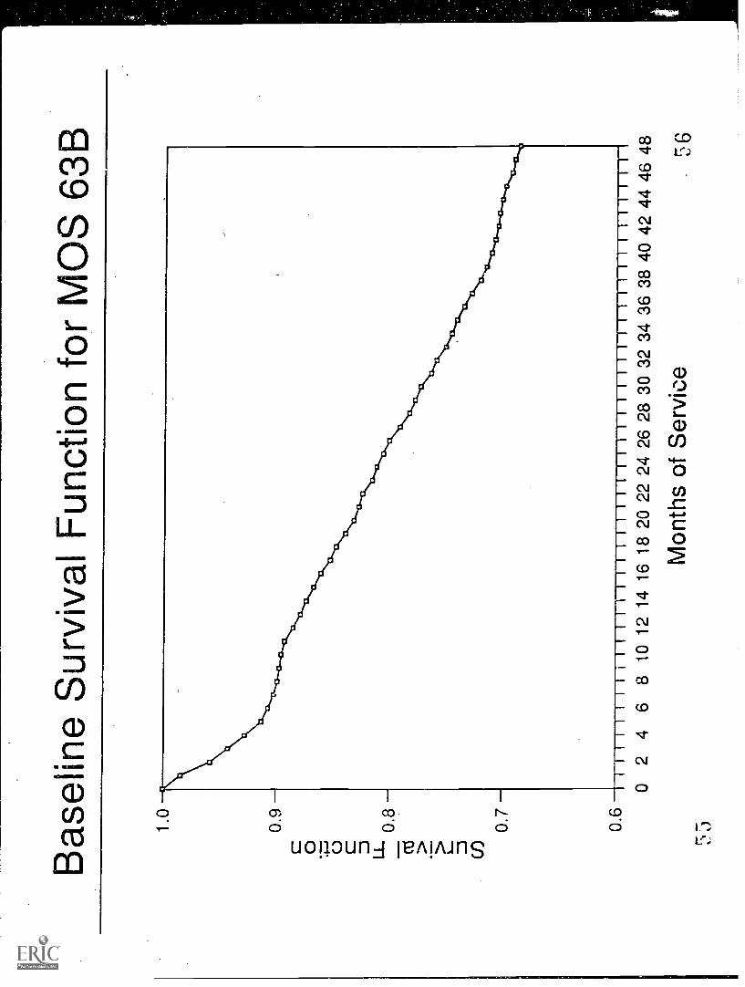
The baseline survivor and hazard functions for one MOS from each
of the fOur job groups are given in Figures 2 through 9.4
- - Insert Figures 2 Through 9 About Here - -
Fitting the proportional hazards models. Because the
hazards proved not to be proportional, a stratified analysis was
conducted where "MOS" wasothe stratifying variable. In a
stratified analysis, the baseline hazards are allowed to differ
for each group, but the regression parameters are assumed to be
the same across groups. That is,
Group 1: In [h(t)] = In [ 1201(t)] + x1 - pkx, (3)Grobp 2: In [h(t)] = In [1202(t)] + p, x - BkA71,
where h01(t) and h02(t) are group-specific hazards that: are not
proportional to each other. This is somewhat analogous to
estimating regression equations that allow group intercepts to
differ while constraining the slopes to be equal across groups.
Whether the hazards are proportional for all groups or only
within stratified groups, the effect of the independent variables
4The survivor and hazard functions are related. The survivor function
can be written
S( t; A717 ) = S0 ( I exP ( )
where XI, is the vector of predictor variables for the nth person, and 50(0 isthe baseline survivor function,
S0(t) = exp(-f ho(u) du)0
1 r-J

First-Term Attrition
15
on the hazard is to shift the baseline hazard up or down,
depending on the values of the variables. More formally, the
effects of the independent variables are multiplicative on the
hazard rate. This may be seen by taking the antilog of equation
1:
h(t). = ho(t) ef3x
In a stratified model, an individual's hazard is shifted up or
down relative to the baseline hazard for their group, whence
equation 4 becomes
(4)
h(t) = hoi(t) ePx (5)
with i being one of g groups (i = 1, . g). The magnitude the
hazard is shifted is the same for all individuals having identical
X vectors, regardless of group membership. The shape of the
hazard that is shifted, however, varies across strata.
Two types of proportional hazard analyses were conducted for
each of the four job groups. The first set of analyses involved
predictor blocks that were entered hierarchically. The first
block contained the four ASVAB composites and the dummy variable
HSDG denoting high-school diploma graduate status (HSDG=1 if a
diploma graduate, zero otherwise). Block one comprises the "base"
variables -- the pre-enlistment variables currently available to
the Army, against which incremental prediction was assessed. As
such, block one was included in all models. Blocks two through
four contained the ABLE, AVOICE, and JOB scores, respectively.
16

First-Term Attrition
16
The incremental fit afforded by each block was assessed relative
to block one. Finally, a model was estimated containing all four
blocks of predictors.
The second type of analysis used a best subset selection
algorithm in the SAS procedure PHREG (SAS Institute, 1992), in
which the best j equations containing k specified predictors is
given. The model considered to be best for a given number of
predictors is the one yielding the highest global score chi-
squared statistic. Here, the best j = 3 equations containing
k = 1, . . . , 26 predictors were obtained. Nested equations were
then selected from the best equations and re-evaluated in PHREG to
obtain the value of -2 Log L for each model. Likelihood ratio
tests were calculated to evaluate the point at which additional
predictors failed to significantly increase the fit of the model.
Stringent p-values were selected, due to the large samples and the
dependence of X2 on sample size. The effect of each variable,
conditional on all other variables in the model, was also taken
into account when deriving the "best" equation for each of the
four groups.
Results
Predictor-Block Models
The results for the five models involving predictor blocks
for each of the four job groups are given in Table 8. (The
parameters for each of the models are given in the Appendix
available from the first author.) The top half of the table
17

First-Term Attrition
17
reports the values of -2 Log L for the five models. (For
stratified analyses, the likelihood, L, maximized for a job group
is the product of each MOS-specific likelihood.) The bottom half
of the table contains likelihood ratio test results (based upon
the values in the top half of the table) for specific model
comparisons.
- - - Insert Table 8 About Here - - -
Consider job group C3 as an example. The value of -2 Log L
for Model 1 (the base variables) is 434.02 with 5 degrees of
freedom (p. < .0001). Clearly, the base variables provide
significant prediction of first-term attrition for soldiers with
three-year terms of enlistment in Combat jobs. Model 2 adds the
12 ABLE measures to the base variables. The value of -2 Log L
increases to 653.08 (again, p. < .0001). To examine whether this
represents a statistically significant increase in the fit of the
model to the data, we calculate the difference between -2 Log L
for the two models. Hence,
. 653.08 -434.02 = 219.06
with (17 - 5) = 12 degrees of freedom. The critical value for x2
at E < .001 is 32.91, indicating that the ABLE provides a
significant increase in model fit. The other values in the bottom
half of Table 8 were calculated similarly.
The results in Table 8 indicate the following:
The base variables are significantly related to
first-term attrition;
13

First-Term Attrition
18
The ABLE provides significant incremental fit to
the base model for all four job groups;
The AVOICE significantly increases the fit-of
the base model for three-year enlistments but
not four-year enlistments; although the sample
sizes differ by a factor of nearly two to one
(N3 = 20,252 and N4 = 10,780), this is probably
not a power issue, given the absolute-size of
each group;
Except for NC3, the JOB does not provide a
statistically significant increase in fit over
the base model;
Addition of the AVOICE and JOB to the ABLE model
increases the fit of the model to the data for
job groups C3 and NC3 (Model 2 vs. Model 5);
again, this is unlikely a power issue.
Thus, the non-cognitive measures improve prediction of
first-term attrition over and above current pre-enlistment
information.
Best Subset Selection
The "variable traces" of the nested models for the best
subset selection analyses are given in Tables 9 through 12, along
with the associated -2 Log L values and differences between them.
All likelihood ratio tests were evaluated as x2 with one degree of
freedom. The tests for groups C3 and NC3 were evaluated relative
9

First-Term Attrition
19
to a critical value of 10.8 (p < .001); tests for groups C4 and
NC4 were evaluated relative to a critical value of 7.9 (n. < .005).
The traces end at the point of the last significant increase in
model fit. All models begin with k = 3 predictors.
- - Insert Tables 9-12 About Here - - - -
Tables 9-12 show that the number of significant predictors
ranges from seven to eleven. No AVOICE or JOB scales appear in
any of the equations. Although the equations are slightly
different across the job groups, seven variables appear in each
best model: high school diploma graduate status, the ASVAB
Quantitative composite, and five ABLE scales (Nondelinquency,
Dominance, Physical Condition, Self Esteem, and Social
Desirability). Indeed, these seven variables constitute the best
equation for both Combat groups.
The parameter estimates and p-values for each best equation
are provided in Tables 13 through 16. To help determine the
conditional impact of each variable on the hazard of first-term
attrition, values of the risk ratio are also provided. The risk
ratio is the exponentiated value of the regression coefficient
(i.e., eb). These values give some insight into the effect of the
independent variables on the criterion, subject to the usual
caveats applied when determining the effect of a predictor on a
criterion in conventional multiple regression analyses based on
the value of the regression coefficients (e.g., Darlington, 1972).
A value less than one indicates a decrease in the hazard rate (the
20

First-Term Attrition
20
regression coefficient is negative);a value greater than one
indicates an increase in the hazard rate.
- - - - Insert Tables 13-16 About Here - - -
The parameters in Tables 13-16 were calculated in the raw
metric of the predictors. Hence, they are analogous to raw
coefficients. As with raw coefficients in conventional
regression, the risk ratio indicates the effect on the hazard
associated with a one unit increase in .the predictor variable.
For example, in the best equation for job group C3; the risk ratio
for Social Desirability of 1.031 signifies that a one unit
increase in the score on this ABLE scale increases the hazard rate
for attrition by 3.1 percent. In the special case of dichotomous
e., duMmy) variables, the risk ratio describes the difference
in the hazard rates for the two groups. For example, the risk
ratio for HSDG of .494 suggests that the hazard rate for high
school graduates is 49.4 percent of that for non-graduates.
Equivalently, the hazard rate for non-graduates is (1/0.494).=
2.024, or 102.4 percent that of high school graduates.
If one wishes to determine the impact on the hazard rate of
an increase of x units (or decrease of -x units), one simply
raises the risk ratio to the power of x (or -x). For example, to
determine the increase on the hazard rate for a five-unit increase
in the Social Desirability score, one computes (1.031)5 = 1.165.
Thus, a five-unit increase in the Social Desirability score
increases the hazard of first-term attrition by 16.5 percent.
21

First-Term Attrition
21
This same approach allows one to determine the effect of a
one standard deviation (a) increase in the measures, which is
equivalent to obtaining standardized regression coefficients. The
metrics of the predictors vary to a considerable degree, even
within the same instrument. Hence, risk ratios based upon one
unit increases could be of little interest. To facilitate metric-
free comparisons, Tables 10 through.13 also contain the values of
the risk ratios raised to the power of a.
The results in Tables 10 through 13 indicate that the
largest conditional effects are quite similar across the four job
groups, with the largest effects provided by the ABLE scales
Nondelinquency and Dominance. A higher Nondelinquency score
translates into a decreased hazard for attrition, whereas the
opposite is true for Dominance. For example, a one unit (standard
deviation) increase in the Nondelinquency score-for Combat
soldiers with three-year enlistments decreases the hazard for
attrition to 95.4 (76.9) percent of its current level.
Equivalently (and perhaps easier to picture), a one unit (standard
deviation) decrease in the Nondelinquency score yields risk ratios
of 1/.954 = 1.048 (1/.769 = 1.300), signifying increases in the
hazard of 4.8 (30.0) percent.5
5The distribution of Nondelinquency is negatively skewed, with a mean forC3 of 47.5, a standard deviation of 5.6, and a maximum value of 60. Thus,
full standard deviation increases in the Nondelinquency scale score might bedifficult to attain for a large number of individuals.
22

First-Term Attrition
Discussion
The results o the event history analysis of first-term
attrition indicate that high school diploma graduate status
remains a very powerful predictor, with the hazard rate for non-
graduates being approximately twice that for graduates.
Nevertheless, information provided by non-cognitive measures
(specifically, scales from the ABLE, a temperament/biodata
inventory) provides significant incremental prediction to pre-
enlistment information currently available to the Army.
Information provided by an interest inventory (the AVOICE) and a
job preference inventory the (JOB) contributed incremental
prediction on occasion, but both were overshadowed when the ABLE
was in the equation.
The results of the block analyses were reasonably consistent
across the four job/enlistment term groups. The best subset
analyses yielded remarkably similar results across the four
groups, identifying six variables that appear in all four "best"
equations and one (the Quantitative composite from the ASVAB) that
appears in three of the four. These seven variables could be
combined to yield a single, highly predictive Army attrition
equation.
Using biodata and temperament inventories as pre-enlistment
selection measures raises questions of the possible effects of
coaching and faking on applicant responses. Biodata items tend to
be less susceptible to such effects to the extent that they are
03
22

First-Term Attrition
23
verifiable. Temperament inventories, however, have been shown to
be easily faked (e.g., Hough, Eaton, Dunnette, Kamp, & McCloy,
1990). Hough et al. found, however, that such distortion does not
have marked effects on the validity of the instrument. To the
extent that this result is generalizable, the concerns about
faking might be exaggerated. Note, however, that the respondents
in the Hough et al. study were not coached.
The effects on the validity of the ABLE of coaching was
investigated by Young, White, and Oppler (1992). Soldiers in this
study were asked to complete the ABLE and were assigned to one of
three response conditions: Honest, Ad-lib Faking (i.e.,
respondents were to answer the questions in a manner each believed
would most impress the Army), and Coached. Soldiers who were
coached were given the same instructions given to the Ad-lib
Faking group, but the respondents were then given three practice
items and instructed which responses were the most favorable and
why. Young et al. examined the effect of the three conditions on
the point-biserial correlations between the ABLE scales and a
dichotomous criterion variable representing attrition during the
first 18 months of service (scored as 1 if attrition occurred, 0
otherwise).
Young et al. (1992) found that the magnitude of the
corrrelations across the thee conditions were similar, with few
significant differences being found between the Honest and Ad-lib
Faking conditions. In this respect, the results are similar to

First-Term Attrition
24
those reported by Hough et al. (1990) with regard to performance
criteria. Virtually all of the point-biserials were negative,
indicating higher ABLE scale scores were associated with decreased
attrition. The point-biserials for the Coached respondents,
however, switched sign, all becoming positive, indicating higher
ABLE scores were associated with increased attrition. Although
Young et al. stated that the reasons for this phenomenon were
uncertain, the study suggests that the impact of coaching on the
validity of the ABLE in an operational setting to screen for
first-term attrition could be severe, although the effects of
coaching might be partially mediated by warnings about scales that
can detect faking, score corrections for faking, and so on.
The use of regression typically raises the question of cross
validity. Event history models do not produce a measure similar
to the coefficient of determination, obviating the use of
shrinkage formulae. Nevertheless, a procedure has been suggested
for assessing the fit of a proportional hazards regression model
in a second sample (McCloy, 1993). To the extent that the
procedure is viable, questions of cross validity may be addressed.
The issue of cross validity, however, has limited
applicability to first-term attrition. Attrition relies in part
on organizational policy that in turn depends upon social,
economic, and political demands. For example, the current
downsizing of the military could result in the Army being a bit
more strict in the enforcement of certain standards for soldiers
J

First-Term Attrition
25
(e.g., minimum performance standards and physical requirements)
than at other times. Optimal equations for predicting attrition
that are developed during the observance of a specific
organizational policy might cross-validate well as long as the
current policy remains the rule. Any change in policy, however,
could result in the inapplicability of the equations. A new
analysis would be required to develop equations for predicting
attrition occurring under the new organizational policy.
The effects of two variables on the hazard of first-term
attrition merit special consideration. Isirst is the positive
relationship between Dominance and the hazard, indicating that
dominant soldiers are more likely to exit prematurely. This
relationship might appear counterintuitive, given that dominance
could be associated with leadership and a "take-charge" demeanor.
Perhaps the finding supports the notion that highly dominant
soldiers are recalcitrant and unresponsive to orders, attempting
to take charge when they should follow.
Of similar interest is the appearance of the ASVAB
Quantitative composite in three of the four best equations. This
composite comprises the two mathematics subtests, Arithmetic
Reasoning (AR) and Mathematical Knowledge (MK). These two
subtests, in turn, appear with the two verbal subtests of Word
Knowledge (WK) and Paragraph Comprehension (PC) in the Armed
Forces Qualification Test, the military's primary selection
measure. As such, soldiers have already been selected to some
26

First-Term Attrition
26
degree on the Quantitative score. The AFQT has been shown time
and again to have very little relationship to attrition, but the
verbal subtests are given twice the weight of the quantitative
subtests when calculating the present AFQT score. By removing the
Quantitative subtests from the AFQT and using them as a composite,
a sizable relationship appears with first-term attrition,
notwithstanding the attenuating effects of range restriction.
Indeed, the lack of relationship between the AFQT and first-
term attrition could be due to the Quantitative and Verbal
subtests working in opposite directions. Whereas higher
Quantitative composite scores are associated with,a decreased
hazard of first-term attrition, the parameters for the Verbal
composite from both the block analyses and the best subset
analyses are positive. Hence, higher Verbal scores are associated
with an increased rate of attrition, with the relationship being
negligible for the Combat MOS but relatively strong for the Non-
Combat jobs.
The current research strongly suggests that the Army can
improve the prediction of first-term attrition by gathering
biodata/temperament information prior to enlistment and by better
using the information they currently possess (i.e., ASVAB
Quantitative scores). Regarding future research, the hazard
functions given in Figures 6-9 indicate that most of the attrition
occurs in the first six months of service. The determinants of
early-term attrition (e.g., during the first six months) may
27BEST COPY AVAILABLE

First-Term Attrition
27
differ from the determinants of attrition occurring later in the
term. Such a hypothesis can be tested using event history
analysis. Future research will be directed at this question, as
well as further investigation into the issue of cross validity.
03

First-Term Attrition
28
References
Allison, P. D. (1984). Event history analysis: Regression for
longitudinal event data (Sage University paper series on
quantitative applications in the social sciences, Number 07-
046). Beverly Hills, CA: Sage.
Campbell, J. P. (Ed.) (1986). Improving the selection,
classification, and utilization of Army enlisted personnel:
Annual report, 1986 fiscal year (Report 813101).
Alexandria, VA: U. S. Army Research Institute.
Campbell, J. P., & Zook, L. (Eds.) (1990a). Improving the
selection, classification, and utilization of Army enlisted
personnel: Final report on Project A (ARI Report 1597).
Alexandria, VA: U. S. Army Research Institute.
Campbell, J. P., & Zook, L. (Eds.) (1990b). Building and
retaining the career force: New procedures for accessing
and assigning Army enlisted personnel (ARI Report 952).
Alexandria, VA: U. S. Army Research Institute.
Campbell, J. P., & Zook, L. (Eds.) (1992). Building and
retaining the career force: New procedures for accessing
and assi nin Arm enlisted sersonnel-- Annual resort 1991
fiscal year (ARI Research Note). Alexandria, VA: U. S.
Army Research Institute.
Cox, D. R. (1972). Regression models and life tables. Journal
of the Royal Statistical Society, 34, 187-202.
Darlington, R. B. (1972). Multiple regression in psychological
29

First-Term Attrition
29
research and practice. Psychological Bulletin, 69(3), 161-
182.
Flyer, E. S. (1959, December). Factors relating to discharge for
unsuitability among 1956 airmen accessions to the Air Force
(WADC-TN-59-201). Lackland Air Force Base, TX: Personnel
Research Laboratory.
Hough, L. M., Barge, B. N., & Kamp, J. D. (1987). Non-cognitive
measures: Pilot testing. In N. G. Peterson (Ed.),
Development and field test of the trial battery for Project
A (ARI Technical Report 739). Alexandria, VA: U. S. Army
Research Institute.
Hough, L. M., Eaton, N. K., Dunnette, M. D., Kamp. J. D., &
McCloy, R. A. (1990). Criterion-related validities of
personality constructs and the effect of response distortion
on those validities. Journal of Applied Psychology, 75(5),
581-595.
Klein, S., Hawes-Dawson, J., & Martin, T. (1991). Why recruits
separate early (R-3980-FMP). Santa Monica, CA: RAND
Corporation.
Knapp, D. J. (1993). Alternative conceptualizations of turnover.
Paper presented at the 101st meeting of the American
Psychological Association, Toronto, Ontario, Canada.
Laurence, J. H. (1993). Education standards and military
selection: From the beginning. In T. Trent and J. H.
Laurence (Eds.), Adaptability Screening for the Armed Forces
30

First-Term Attrition
30
(pp. 1-40). Washington, DC: Office of the Assistant
Secretary of Defense.
Lawless, J. F. (1982). Statistical models and methods for
lifetime data. New York: John Wiley & Sons.
McBride, J. R. (1993). Compensatory screening model development.
In T. Trent and J. H. Laurence (Eds.), Adaptability
Screening for the Armed Forces (pp. 1-40). Washington, DC:
Office of the Assistant Secretary of Defense.
McCloy, R. A. (1993). An overview of survival analysis. Paper
presented at the 101st meeting of the American Psychological
Association, Toronto, Ontario, Canada.
McCloy, R. A., Harris, D. A., Barnes, J. D., Hogan, P. F., Smith,
D. A., Clifton, D., & Sola, M. (1992). Accession Quality,
job performance, and cost: A cost-performance tradeoff
model (FR-PRD-92-11). Alexandria, VA: Human Resources
Research Organization.
McHenry, J. J., Hough, L. M., Toquam, J. L., Hanson, M. A., &
Ashworth, S. (1990). Project A validity results: The
relationship between predictor and criterion domains.
Personnel Psychology, 43, 335-354.
Peterson, N. G., Hough, L. M., Dunnette, M. D., Rosse, R. L.,
Houston, J. S., Toquam, J. L., & Wing, H. (1990). Project
A: Specification of the predictor domain and development of
new selection/classification tests. Personnel Psychologv,
43, 247-276.

First-Term Attrition
31
Singer, J. D., & Willett, J. B. (1991). Modeling the days of our
lives: Using survival analysis when designing and analyzing
longitudinal studies of duration and the timing of events.
Psychological Bulletin, 110(2), 268-290.
Steinhaus, S. D. (1988). Predicting military attrition from
educational and biographical information (FR-PRD-88-06).
Alexandria, VA: Human Resources Research Organization.
Trent, T. (1993). The Armed Services Applicant Profile (ASAP).
In T. Trent and J. H. Laurence (Eds.), Adaptability
Screening for the Armed Forces (pp. 71-99). Washington, DC:
Office of the Assistant Secretary of Defense.
Waters, B. K., Barnes, J. D., Foley, P., Steinhaus, S. D., &
Brown, D. C. (1988). Estimating the reading skills of
military applicants: Development of an ASVAB to RGL
conversion table (FR-PRD-88-22). Alexandria, VA: Human
Resources Research Organization.
White, L. A., Nord, R. D., Mael, F. A., 4 Young, M. C. (1993).
The Assessment of Background and Life Experiences (ABLE).
In T. Trent and J. H. Laurence (Eds.), Adaptability
Screening for the Armed Forces (pp. 101-162). Washington,
DC: Office of the Assistant Secretary of Defense.
Young, M. C., White, L. A., & Oppler, S. H. (1992). Effects of
coaching on validity of a self-report temperament measure.
Proceedings of the 34th Annual Conferences of the Military
Testing Association (pp. 188-193). San Diego, CA.
02

First-Term Attrition
Table 1
Summary of the 21 Army MOS
32
MOS Name of Job MOS Name of Job
11B Infantryman 55B Ammunition Specialist
12B Combat Engineer 63B Light-Wheel VehicleMechanic
13B Cannon Crewman67N Utility Helicopter
16S MANPADS Crewman Repairer
19E M60 Armor Crewman 71L AdministrativeSpecialist
19Ka M1 Armor Crewman 76Y Unit Supply Specialist
27E Tow/Dragon Repairer 88M Motor TransportOperator
29E Comm.-Electronics Radio Repairer91A Medical Specialst
31C Single Channel Radio Repairer94B Food Service Specialist
51R Carpentry/Masonry Specialist95B Military Police
54B NBC Specialist96B Intelligence Analyst
a MOS 19E and 19K differ only in terms of equipment (i.e., type of tank).
23

First-Term Attrition
33
Table 2
Sample sizes, number and percentage of attritions, and number and
percentage of censored observations for Soldiers with Three-Year
Enlistments in Combat Jobs (C3)
MOS N Events Censored Observations
N Percentage N Percentage
11B 4,875 1,354 27.8 3,521 72.2
12B 1,131 295 26.1 836 73.9
13B 2,416 729 30.2 1,687 69.8
16S 410 140 34.1 270 65.9
19E 287 91 31.7 196 68.3
19K 570 128 22.5 442 77.5
TOTAL 9,689 2,737 28.2 6,952 71.8
34

First-Term Attrition
34
Table 3
Sample sizes, number and percentage of attritions, and number and
percentage of censored observations for Soldiers with Four-Year
Enlistments in Combat Jobs (C4)
MOS N Events Censored Observations
N Percentage N Percentage
11B 4,196 1,397 33.3 2,799 66.7
12B 247 73 29.6 174 70.4
13B 1,227 405 33.0 822 67.0
16S 81 16 19.7 65 80.3
19E 123 47 38.2 76 61.8
19K 566 186 32.9 380 67.1
TOTAL 6,440 2,124 33.0 4,316 67.0
25

First-Term Attrition
35
Table 4
Sample sizes, number and percentage of attritions, and number and
percentage of censored observations for Soldiers with Three-Year
Enlistments in Non-Combat Jobs (NC3)
MOS N Events Censored Observations
N Percentage N Percentage
54E 566 149 26.3 417 73.7
55B .198 73 36.9 125 63.1
64C 169 247 32.1 522 67.9
71L 1,341 362 27.0 979 73.0
76Y 518 115 22.2 403 77.8
91A 2,685 649 24.2 2,036 75.8
94B 1,579 547 34.6 1,032 65.4
95B 2,907 619 21.3 2,288 78.7
TOTAL 10,563 2,761 26.1 6,952 73.9
26

First-Term Attrition
36
Table 5
Sam le sizes number and ercenta e of attritions and number and
percentage of censored observations for Soldiers with Four-Year
Enlistments in Non-Combat Jobs (NC4)
MOS N Events Censored Observations
N Percentage N Percentage
27E 104 28 26.9 76 73.1
29E 188 50 26.6 138 73.4
31C 390 143 36.7 247 63.3
51B 319 88 27.6 231 72.4
63B 1,353 419 31.0 934 69.0
67N 277 55 19.9 222 80.1
76Y 874 275 31.5 599 68.5
94B 429 179 41.7 250 58.3
95B 406 99 24.4 307 75.6
TOTAL 4,340 1,336 30.8 3,004 69.2
27

First-Term Attrition
Table 6
The Eleven Substantive ABLE Scales
37
Emotional Stability
Self-Esteem
Cooperativeness
Conscientiousness
Nondelinguency
Traditional Values
Work Orientation
Internal Control
Energy Level
Dominance
Physical Condition
2 3

First-Term Attrition
Table 7
38
The Six AVOICE Composites and Their Constituent Scales
AVOICE Composite AVOICE Scales
Administrative Clerical/Administrative
Warehousing/Shipping
Audiovisual Arts Aesthetics
Audiographics
Drafting
Food Service Food Service (Employee)
Food Service (Professional)
Interpersonal Leadership/Guidance
Medical Services
Protective Services Fire Protection
Law Enforcement
Rugged/Outdoors Combat
Firearms Enthusiast
Rugged Individualism
Skilled/Technical Computers
Electronic Communications
Mathematics
Science/Chemical
Structural/Machines Electronics
Heavy Construction
Mechanics
Vehicle/Equipment Operator
29

Table 8
Results for the five models involvin
job groups
Values of -2 Log L
First-Term Attrition
redictor blocks for each of the four
Job Group
39
Model df C3 C4 NC3 NC4
(1) Base 5 434.02 188.48 329.72 102.30
(2) Base + ABLE 17 653.08 330.67 649.52 272.58
(3) Base + AVOICE 13 478.96 207.32 352.78 115.67
(4) Base + JOB 8 444.08 198.97 356.95 105.05
(5) Base + ALL 28 693.84 351.96 69.0.04 284.40
Values of -2 Log (L2 - L1)
Model
Comparisons df
Job Group
C3 C4 NC3 NC4
1 vs. 2 12 219.0u 142.19 319.80 170.28
1 vs. 3 8 44.94 18.84ns 23.06' 13.37ns
1 vs. 4 3 10.06ns 10.49ns 27.23 2.75ns
1 vs. 5 23 259.82 163.48 360.32 182.10
2 vs. 5 11 40.76 21.29ns 40.52 11.81ns
3 vs. 5 15 214.88 144.64 337.26 168.73
4 vs. 5 20 249.76 152.99 333.09 179.35
All values significant at 2 < .001 except 2 < .01 and ns non-significant.

First-Term Attrition
Table 9
Variable traces and fit statistics of the nested models for, the
best subset selection analyses: Job Group C3 (n = 9,689)
Model -2 Lop Lz2 (df
=1)
HSDG, QUANT, Nonda 41,353.64
+ Dominance 41,328.84 24.80
+ Physical Condition 41,310.58 18.26
+ Social Desirability 41,290.80 19.78
+ Self Esteem 41,277.66 13.14
Significant x2 Values, df = 1: g < .001 = 10.83
aABLE scale Nondelinquency
41
40

First-Term Attrition
41
Table 10
Variable traces and fit statistics of the nested models for the
best subset selection analyses: C4 (n = 6,440)
Model -2 LOCI L
HSDG, QUANT, Nonda 31,667.26
+ Dominance 31,651.36 15.90
+ Self Esteem 31,631.08 20.28
+ Social Desirability 31,620.74 10.34
+ Physical Condition 31,610.32 10.42
Significant X2 Values, df = 1: 2. < .005 = 7.88
aABLE scale Nondelinquency
42

First-Term Attrition
42
Table 11
Variable traces and fit statistics of the nested models for the
best subset selection analyses: Job Group NC3 (n = 10,563)
Model -2 Loq L /2 (df = 1)
HSDG, QUANT, Conda 39,482.91
+ Nondelinquency 39,411.01 71.90
+ TECHNICAL 39,387.20 23.81
+ VERBAL 39,358.51 28.69
+ Social Desirability 39,325.83 32.68
+ Emotional Stability 39,302.77 23.06
+ Dominance 39,269.28 33.49
+ Energy Level 39,253.28 16.00
+ Self Esteem 39,236.97 16.31
Significant x2 Values, df = 1: Q < .001 = 10.83
aABLE scale Physical Condition
43

First-Term Attrition
43
Table 12
Variable traces and fit statistics of the nested models for the
best subset selection analyses: NC4 (n = 4,340)
Model -2 LOP L y2 (df = 1)
HSDG, Nond, Conda 16,564.75
+ Dominance 16,534.93 29.82
+ TECHNICAL 16,518.38 16.55
+ VERBAL 16,506.40 11.98
+ Social Desirability 16,491.86 14.54
+ Self Esteem 16,482.54 9.32
Significant x2 Values, df = 1: p < .005 = 7.88
aABLE scale Physical Condition
44

First-Term Attrition
44
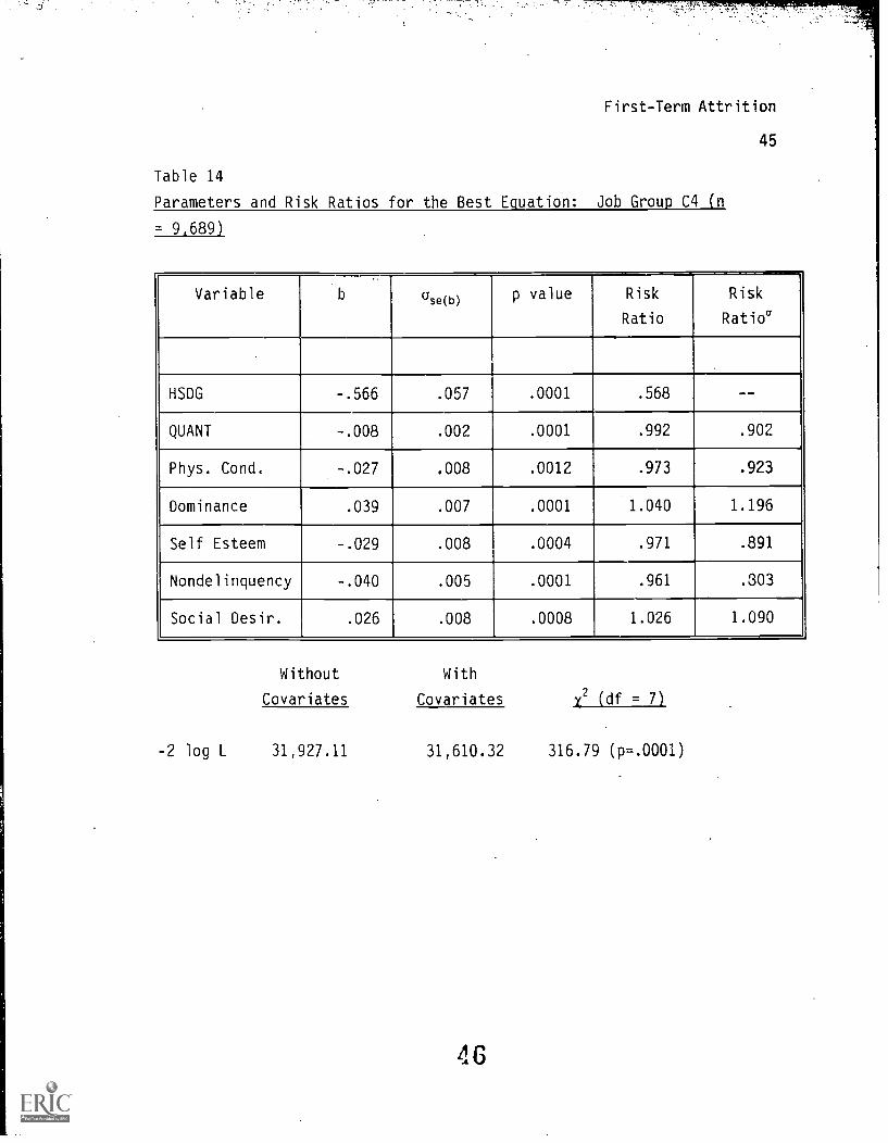
Table 13
Parameters and Risk Ratios for the Best Equation: Job Group C3 (n
= 9,689)
Variable b crse(b) p value Risk
Ratio
Risk
Ratios
HSDG -.705 .045 .0001 .494 --
QUANT -.013 .002 .0001 .987 .836
Phys. Cond. -.023 .008 .0014 .976 .933
Dominance .039 .006 .0001 1.040 1.194
Self Esteem -.026 .007 .0003 .974 .903
Nondelinquency -.047 .004 .0001 .954 .769
Social Desir. .030 .007 .0001 1.031 1.113
Without With
Covariates Covariates 72 (df 7)
-2 log L 41,907.32 41,277.66 629.66 (p=.0001)
J
First-Term Attrition
45
Table 14
Parameters and Risk Ratios for the Best Equation: Job Group C4 In
= 9,689)
I Variable b ase(b) p value Risk
Ratio
Risk
Ratio'
HSDG -.566 .057 .0001 .568 --
QUANT -.008 .002 .0001 .992 .902
Phys. Cond. -.027 .008 .0012 .973 .923
Dominance .039 .007 .0001 1.040 1.196
Self Esteem -.029 .008 .0004 .971 .891
Nondelinquency -.040 .005 .0001 .961 .303
Social Desir. .026 .008 .0008 1.026 1.090
-2 log L
Without With
Covariates Covariatesx2 (df 7)
31,927.11 31,610.32 316.79 (p=.0001)
46

First-Term Attrition
46
Table 15
Parameters and Risk Ratios for the Best Equation: Job Group NC3
In = 10,563)
Variable b ase(b) p value Risk
Ratio
Risk
Ratio'
HSDG -.712 .054 .0001 .491 --
QUANT -.012 .002 .0001 .989 .858
TECH -.010 .001 .0001 .990 .835
VERBAL .014 .002 .0001 1.014 1.165
Phys. Cond. -.066 .007 .0001 .936 .816
Dominance .032 :006 .0001 1.032 1.157
Energy Level .026 .005 .0001 1.027 1.169
Self Esteem -.030 .008 .0001 .970 .887
Nondelinquency -.039 .004 .0001 .962 .808
Emotional Stab. ..036 .007 .0001 1.037 .833
Social Desir. -.033 .005 .0001 .968 1.128
Without With
Covariates Covariates2
= 11)
-2 log L 39,877.43 39,236.97 640.46 (p=.0001)
47

First-Term Attrition
47
Table 16
Para2ters and Risk Ratios for the Best Equation: Job Group NC4
(n = 4,340)
Variable b ase(b) p value Risk
Ratio
Risk
Ratio°
HSDG -.568 .084 .0001 .567 --
TECH -.011 .002 .0001 .989 .824
VERBAL .013 .003 .0001 1.013 1.163
Phys. Cond. -.067 .010 .0001 .935 .816
Dominance .046 .008 .0001 1.047 1.239
Self Esteem -.031 .010 .0022 .970 .887
Nondelinquency -.046 .006 .0001 .955 .779
Social Desir. .038 .009 .000 1 1.038 1.136
Without With
Covariates Covariates Y2 (df 8)
16,726.49 16,482.54 243.95 (p=.0001)
4 3

First-Term Attrition
48
Figure Caption
Figure 1. Formation of the four ASVAB composite scores from the
ASVAB subtests.
Figure 2. Baseline survivor function for MOS 11B.
Figure 3. Baseline survivor function for MOS 13B.
Figure 4. Baseline survivor function for MOS 63B.
Figure 5. Baseline survivor function for MOS 95B.
Figure 6. Baseline hazard function for MOS 11B.
Figure 7. Baseline hazard function for MOS 13B.
Figure 8. Baseline hazard function for MOS 63B.
Figure 9. Baseline survivor function for MOS 95B.
40

Mechanical Comprehension
Auto Shop
Electronics Information
Math Knowledge
Arithmetic Reasoning
Verbal
General Science
Coding Speed
Number Operations
Note: From Campbell (1986), p. 4-16.
50
First-Term Attrition
Technical
Quantitative
Verbal
Speed
49

Bas
elin
e S
urvi
val F
unct
ion
for
MO
S 1
1B
0.6
51
11
11
11
11
11
11
11
11
11
11
11
11
11'
11
11
11
11
11
11
11
11
11
1
02
46
8 10
12
14 1
6 18
20
22 2
4 26
28
30 3
2 34
36
38 4
0 42
44
46 4
8
Mon
ths
of S
ervi
ce52

Bas
elin
e S
urvi
val F
unct
ion
for
MO
S 1
3B
1.0
0.6
0
t
24
68
1012
1416
18 2
022
24 2
6 28
30
3234
36
Mon
ths
of S
ervi
ce
Bas
elin
e S
urvi
val F
unct
ion
for
MO
S63
B
0.6
1111
111
IIIIII
IIIII1
1111
1111
1111
1111
IIIIIi
II11
02
46
8 10
12
14 1
6 18
20
22 2
4 26
28
30 3
2 34
36
38 4
0 42
44
46 4
8
Mon
ths
of S
ervi
cer6

Bas
elin
e S
urvi
val F
unct
ion
for
MO
S 9
5B
1.0
0.9
-c 0 LL
0.8
-
0.7-
-
0.6
--r-
iI
I
57
II
11
11
I1
II
11
I1
11
I1
11
I1
I1
I1
I1
11
I
02
46
810
1214
1618
2022
2426
28
3032
34 3
6
Mon
ths
of S
ervi
ce

Bas
elin
e H
azar
d F
unct
ion
for
MO
S 1
1B
0.04 0.03
-c 0
0.02
N(11
cti
0.01
0.00
IIIIIIIII111111IIIIIIIIIII1111IIII II11I1I1IIII
24
68
10 1
2 14
16
18 2
0 22
24
26 2
8 30
32
34 3
6 38
40
42 4
4 46
48
Mon
ths
of S
ervi
ce60

Bas
elin
e H
azar
d F
unct
ion
for
MO
S13
B
0.04
0.03
0 0
0.02
N I-2
0.01
0.00
El
11
11
11
11
11
11
1 11
1111
1-T
-1I
I 11
1111
111
24
68
1012
1416
1820
2224
2628
3032
3436
Mon
ths
of S
ervi
ceC
2

Bas
elin
e H
azar
d F
unct
ion
for
MO
S 6
3B
0.04
0.03
-c 0 0 C D Li-
0.02
-2 (II N ai I 0.
01 -
0.00
C3
11
I1
I1
i1
11
11
11
11
11
11
11
11
11
11
11
11
11
11
11
11
11
11
11
24
68
1012
1416
1820
2224
2628
3032
3436
3840
4244
46
Mon
ths
of S
ervi
ce
48 C4

Bas
elin
e H
azar
d F
unct
ion
for
MO
S 9
5B
0.04
0.03
c O c 1-1-
-0.
02
N I-2 cti
0.01
0.00
F5
II
I1
II
Il
Ii
1I
ii
11
11
11
II
II
II
II
II
24
68
1012
1416
1820
2224
2628
3032
3436
Mon
ths
of S
ervi
ce