Location of manufacturing FDI in Hungary: Howimportant are business-to-business relationships?∗

Gábor BékésCentral European UniversityBudapest, Nádor utca 7., Hungary

June 23, 2004

Abstract

Contributing to the new economic geography literature, this papersets up a simple model with monopolistic competition and estimatesthe determinants of location choice. This research addresses three cen-tral questions: Is there an agglomeration effect strong enough to ex-plain co-location? Does market access matter for the location of foreigninvestment even within a small country? Are input-output linkagesthe key motive for location? In this paper, I apply a discrete choicemethodology to find out to what extent various factors like wages ormarket access influence location choice within one country. I use twodetailed datasets of Hungarian firms and wages between 1992 and 2001considering all the new-born companies in manufacturing with foreignownership.JEL classification: F23, R3, R55Keywords: economic geography, industrial location, FDI, regional

policy, discrete choice models

1 Introduction

Over the past twenty years, study of international location of productionand trade has gone through a remarkable development. New trade theoryin the eighties, and economic geography in the nineties offered new modellingtechniques and economic explanations. Geographical location was placed inthe centre of thinking as a new breed of models on urban, regional andinternational economics of agglomeration were developed.

Economic geography, simply put, is "all about where economic activitytakes place - and why" (Fujita, Krugman and Venables [1999, p.14.]). Mod-els aim at explaining cross regional agglomeration patterns amid transaction

∗This is work in progress and is not to be quoted. For comments and suggestions Ithank Gianmarco Ottaviano, Laszlo Halpern, Fabrice Defever and Almos Telegdy.

1

costs of doing interregional business. The subject has relevance both at afirm level and at macro level. At the firm level, it gives arguments for lo-cation decisions including moving into a foreign region, following peers andbusiness partners or being a pioneer in an unknown area. At a macro levelit helps understanding dissimilar regional development patterns or causesof backwardness. It also helps see what happens when regions come closeras market integration proceeds or new motorways are built. Importantly,it may give new consideration for policymakers when deciding on regionaldevelopment policy.

In Central and Eastern Europe rapid changes and restructuring in man-ufacturing have taken place since 1990. Thus, countries like Hungary offer alaboratory experiment to study the geographic properties of a large numberof new investments by firms entering a region previously closed to foreign-ers. As for the development, foreign direct investment was instrumental intransforming the industry of transition economies. In Hungary, for exam-ple, the stock of FDI reached 40% of GDP by 2003. The rapid appearanceof foreign-owned manufacturing sites offers a great opportunity: studyingthe geographic properties of a large number of new firms entering a regionpreviously closed to foreigners.

In this paper I will consider foreign direct investments in Hungary andinvestigate why the presence of a firm has an impact on investment byanother. This research addresses three central questions: Is there an ag-glomeration effect strong enough to explain co-location? Within a smallcountry does market access matter for the location of foreign investment?Are input-output linkages the key motive for location? In this study, I ap-ply a discrete choice methodology to find out to what extent factors likewages or input-output linkages influence location choice within one country.I use two detailed datasets of Hungarian firms and wages between 1992 and2001 and I consider all the new-born manufacturing companies with foreignownership.

The paper is organised as follows. First I summarize the related liter-ature analysing results of firm location in general and FDI location specif-ically. Second, I present a small model of location choice. Third I reportkey findings about location choice within a country, describe the empiricalmethod and the data to be used. Finally, the results of the empirical inves-tigation are presented and a few points for economic policy are made. Forthis paper is a work in progress, ideas for future research are noted, too.

2 Related literature

2.1 The economic geography contribution

With recent developments in new economic geography (or NEG) modelling,location theory experienced a marked revival. Over the past two centuries,

2

from von Thünen through Marshall to Krugman, serious efforts have beeninvested into studying locational patterns of firms. The key trade-off firmshave to bear in mind was established by von Thünen as early as 1826:being close to customers versus being close to the source of inputs. Further,the fact that the transportation cost is of paramount importance was laiddown a century ago. Also, the key idea that firm location depends on theproximity of demand was introduced a long ago by Harris [1954] who devisedthe simplest aggregate market-potential function.

2.1.1 Basic intuition

By the neoclassical model of economics textbook, economic activity is spreadout evenly through space since the flow of production factors levels out dif-ferences in development and prices alike. Wherever there is a scarcity inone good or factor, its relative price will be higher making it worthwhileto ship goods from other places in the world as long as prices are equal-ized. Equalisation may be reached via trade and/or capital investment andlabour migration. It is easy to see that this is not the case in reality: thereis a concentration of activity in cities, industrial or financial centres, andthere is a marked difference between developed and underdeveloped regionseven within one country. There are many reasons for the concentration ofproduction (i.e. marked co-location of firms) and models of new economicgeography aim at uncovering the essential reasons behind both agglomera-tion and dispersion of economic activity.

Let us give here a bit of economic intuition that lies behind these the-ories. Most of the models assume that firms produce with an increasingreturns to scale technology, market transactions are costly and these costsdetermine whether firms benefit from settling close to one another therebygiving rise to agglomerations. In the lack of transaction (trade) costs, pro-duction would be determined by supply side consideration (such as efficientscale size) only. However, if transportation is costly, demand side becomesa determining factor of location choice given that being close to customersyields lower operating costs. Accordingly, a shift in transaction costs maylead to relocation of industries as both optimal level of concentration andoptimal distance from customers is altered.

To better grasp the key ideas of the new economic geography, let usconsider a simple framework with two regions (e.g. as in Fujita, Krugmanand Venables [1999, Chapter 4]). Firms can decide whether to settle inone region, the other one or in both. Let us see what are the forces inthe economy that determine concentration or dispersion of firms and theiractivity.

Let us start with one region having slightly more firms than the other.The more firms are present in a region the more easily can they find therequired intermediate goods locally. Hence, there is a lower import share

3

and saving in transport costs will make final prices lower, too. Greatercompetition among firms will also lead to higher wages that, along with lowerprices help raise living standards. Better prospects will magnet migrantsfrom the other region and the labour pool will rise. This will lower wagesto some extent but the size of the market will rise thus helping firms tosell more allowing to lower prices. Also, greater market (more customerslocally and the possibility to make an even better use of increasing returnsto scale) will make new firms enter the region. Thus, in this case labourmarket development and capital flows reinforce each other: efficiency ofproduction and stronger purchasing power of customers will offset risingwages and agglomeration forces lead to a growing concentration of activity inone region. This is what Nobel-laureate Gunnar Myrdal dubbed “cumulativecausation” (Myrdal [1957])

Of course, agglomeration forces do not prevail without boundaries, thereare dispersion forces in action, too. First and foremost, high wages will makecertain wage-sensitive industries incapable to offset rising costs. These com-panies will at some point opt to locate in the other region. Although theywill face much higher transaction costs when selling to the larger (and richer)region, but production costs will be much lower in the other region. Anotherreason to move is falling final prices as a result of greater competition. Inthis case, benefits of lower competition in the other region will offset disad-vantages of loosing suppliers and some customers in the larger region. As wehave seen, the size of transaction costs and thus the distance between mar-kets plays a pivotal role. Note, that remoteness does not only incorporatephysical distance “ as the crow flies” but also the quality of transport net-work, language and cultural barriers, differences in corporate managementstyles or regulatory environment.

An excellent survey of key hypotheses emerging from models of neweconomic geography and their mixed empirical support can be found inHead and Mayer [2003a].

2.1.2 Focus on location choice

Over the past few decades there has been a renewed interest in location the-ory. Indeed, in the age of cheap transportation costs and complex productionmethods as well as business to business relationships, it emerged that “newfirms have a high propensity to settle at places where economic activitiesare already established” as posited in Ottaviano, Tabuchi and Thisse [2003,p.7.].

New economic geography models have been employed to explain locationof overall economic activity by Krugman [1991], industrial clusters in Fujita,Krugman and Venables [1999, Ch. 16.], location of various manufacturingsectors by Midelfart-Knarvik, Overman and Venables [2000]or individualsectors such as those of accordions by Robert-Nicaud [2002, Ch. 5]. Further,

4

a multi-regional setting was soon applied to the NEG models. Krugmanextended his earlier model to have multiple regions and the core-peripherymodel was extended in the Fujita, Krugman and Venables [1999, Ch. 16.]volume to have three, four, or many regions.

The notion that inter-company sales should be taken into account ismore recent but input-output (I-O) linkages were incorporated into the neweconomic geography models about a decade ago. In the literature there aretwo distinct ways to introduce I-O linkages. Venables [1996] posits that thereare downstream and upstream industries per se and there is a flow of goodsbetween these two. The other stream, initiated by Krugman and Venables[1995] considers a single imperfectly competitive industry where the finalgood of one firm is the intermediate good of an other. Here, the purchaseof intermediate goods enters the cost function via a composite price indexof such products, while demand is augmented with corporate purchasingpower. Input-output linkages appeared in some recent work by Ottavianoand Robert-Nicaud [2003] who compared the theoretical as well as welfareimplications of I-O models in comparison with labour migration.

In the vertical linkage models centrifugal and centripetal forces lead tothe emergence of two important externalities. First, when a firm entersa region and starts production, it also increases the demand for upstreamactivities thus expanding the home market. Second, it also increases localsupply of downstream output, leading to the so called market crowdingeffect. These two forces work against each other, and agglomeration takesplace when market expansion effect dominates the market crowding effect.

There are other drivers of industrial clustering. One such reason thatmakes worth locating close to one another is the potential of knowledge spill-over. This is true for human as well as physical capital. The attraction towork close to other people is noted in Marshall [1920] and the importanceof face to face communication is discussed in Leamer and Stolper [2000]. Asfor firms, proximity allows to exchange inventions while technology spillovershelp increase productivity using other firms’ knowledge.

Another such agglomeration force is labour pooling: firms enjoy thepresence of a larger set of labour where the specific knowledge required bythe firm, may just be fished out easily Amiti and Pissarides [2001]. In atransition economy, one reason for settling where the old industrial baseused to operate may be the presence of such labour pool.

Market potential has been first investigated in an international context;proximity to key markets and suppliers have explicitly featured in empiricalworks explaining overall economic activity or per capita income. Reddingand Venables [2001] argues that a country’s wage level (proxied by per capitaincome) is dependent on its capacity to reach export markets and manageto get hold of the necessary intermediate goods cheaply. For the EuropeanUnion, Head and Mayer [2003b].look at Japanese investments. Results showthat apart from a very important market potential measure, a number of

5

traditional explanatory variables (e.g. taxes) and agglomeration variablesturn to be significant.

2.2 Location of FDI within a country

Location of industry and more specifically that of the foreign-owned manu-facturing has long been in the limelight of economic research. Mainstreaminternational economics focused on the interaction of direct investment andinternational trade. The interest in intra-national location choice, inspiredby the marriage of international and urban/regional economics, is more re-cent.

Various studies have researched location choice of foreign investors, mostlyin manufacturing, using some version of a discrete choice model. An inspir-ing piece is Crozet, Mayer and Mucchielli [2003] who study location of FDIin France. They use a simple model of oligopolistic competition and a con-ditional logit model to simulate corporate choice of location. They find thatfirms of the same nationality like to group together, locations close to homecountry are chosen more frequently, and some industries (like car plants)have a strong tendency to agglomerate. The authors also find that firms ofthe same nationality like to settle close to one another. Similarly, a studyby Head and Ries [1999] looks at Japanese investments in the US and findsthat firms belonging to the same keiritsu tend to settle close to each other.

Agglomeration has been indeed found to be an important determinantof location in developed countries. Coughlin and Segev [2000] looked at thegeographic features of employment of newly established foreign owned plantsin US states. They found that “size, labour force quality, agglomerationand urbanization economies, and transportation infrastructure are foundto affect positively the location of new foreign-owned plants, while unitlabour costs and taxes are found to deter new plants”. For example theagglomeration effect was proved to be especially important in explainingthe attractiveness of the Southeast region. In a similar study, Coughlinand Segev [1999] considered FDI in China finding location to be important(proximity to the Coast) but transportation infrastructure (thus costs) tohave a negligible impact only. Given the concentration of FDI in regionsthat contain the preferential zones created in the early eighties, the "historymatters" argument (i.e. in the presence of virtuous circles, a small differencebetween regions may give an ever increasing advantage to the slightly betterone) found some support, too.

Barrios, Strobl and Gorg [2002] look at multinationals’ location choicein Ireland with special interest in the role of agglomeration forces as wellas state support. They find that agglomeration forces contributed substan-tially to location choices but proximity to major ports and airports wasalso helpful. More importantly they find evidence that higher public in-centives in designated areas have increased the probability of multinational

6

investment. According to the results, regional policy has been effective inattracting low-tech multinationals to the designated areas.

Anecdotal evidence confirms that agglomeration forces are active in tran-sition economies of Central and Eastern Europe (CEE). The presence of in-dustrial clusters is an easy to spot feature of new manufacturing base in theregion, including the motor vehicle cluster in North-West Hungary, WestSlovakia or South-West of the Czech Republic. Also, there is some evidenceshowing that large multinationals lured in their usual suppliers1.

Results with data on developing or transition economies have just startedto emerge of late. Disdier and Mayer [2003] compares French investment inWestern and Eastern part of Europe. They find that location choice ispositively influenced by local demand and proximity to France increases theprobability of the given country being chosen. Cieslik [2003] used a Poissonmodel on 50 Polish regions to find that proximity of key export targets,industry and service agglomeration and road network are the key magnetsfor foreign investment.

As for Hungary, Fazekas [2003] looked at the concentration of FDI from alabour market point of view to study what impact capital inflow had on theregional structure of the country. The paper finds that concentration patternof foreign-owned enterprises (FE) is just marginally higher (and unchangedthrough time) than that of the domestically owned (DE) ones. However, FEsare concentrated in a different pattern, being located closely to the Westernborder. Then, Fazekas estimates a regression of the concentration indicesbeing dependent of education, industrial base and distance from the border.He finds significant coefficients with the expected signs. My approach issomewhat different of Fazekas [2003] in that I only concentrate on FDI andinvestigate the agglomeration patterns of these firms.

Barta [2003] describes regional differentiation in post-transition Hungary.She gives two good examples of agglomeration forces in work. In Centraland Eastern Europe manufacturing of electronic devices by firms such asFlextronics can be found in a fairly narrow band from north Poland throughthe Czech Republic, West Slovakia, West and Central Hungary down toNorth Slovenia and Croatia. In Hungary, suppliers to the car plant of Suzukiare shown to be settled in neighbouring counties of Komarom-Esztergommegye, where the Suzuki plant is located. Further, second wave of suppliersthat settled directly to service the plant are on average much closer to thefactory than the suppliers during the first half of the nineties.

1The latest example is Hyundai motors in Slovakia where eight other Korean firmsannounced to follow Hyundai.

7

3 The model with I-O linkages

In this model we put an emphasis on business to business relations. Themain relationship between any two firms is a potential of supplier-buyer link,i.e. one firm’s output is the intermediate good of another. Modelling andmeasuring this potential will be in the centre of this analysis. The model isusing the "classic" ingredients of new economic geography or Dixit-Siglitzt-Krugman (referred as DSK) world: Cobb-Douglas utilities and a marketstructure á la Dixit and Stiglitz [1977]. One key aspect of firm-to-firmrelationship here is related to input-output linkages that were introducedby Krugman and Venables [1995] in order to model the fact that firms sellgoods not only to consumers but other firms as well. This paper followsthe concise display of multi-country and multi-industry model in Fujita,Krugman and Venables [1999, Chapter 15A].

3.1 Market structure

There is monopolistic competition in all sectors producing a range of differ-entiated goods. We focus on manufacturing and overlook agriculture here.True, we will miss a dispersion force but hope that wages and local consumerdemand will be enough, owing to very limited migration.

There are r = 1...R regions, j = 1...J industries, with njr firms producinga variety each of industry j in region r.

Each consumer enjoys manufacturing goods and the composite good con-sumed comes from a constant elasticity of substitution (CES) function of theavailable varieties. The elasticity of substitution between goods is measuredby σj . Theoretically it measures to what extent goods are close to eachother, i.e. whether consumers are easily willing to replace one with an-other. If it is small, products differ, in case of σj = ∞, the products arehomogenous, and the market structure is identical to perfect competition.

Importantly, all firms use a set of goods produced by other industriesthat are aggregated by a CES subutility function into a composite good.The intermediate good price index, Gj

r denoting the minimum cost of pur-chasing a unit of this composite good, is a key variable in this setup for firmsbenefit from supplier proximity. If more of necessary intermediate goods areproduced locally, less transportation cost will have to be paid, hence pro-duction costs will be lower, too. This creates a forward linkage. Here, theintermediate price index is weighted average (with njl being the number of

relevant firms2) of f.o.b. prices³pjl τ

jl_r

´that already include an iceberg

type transport costs, τ jl_r ≥ 1: (i.e. when τ jl_r = 1 for the home regiononly, l = r).

2Later, the number of firms may be replaced with volume of output.

8

Gjr =

"RXl=1

njl

³pjl τ

jl_r

´1−σj# 11−σj

(1)

This way of entering the price index implies the love of variety effect.The intermediate price index for a firm in industry j of region r is Gj

r, whereioij is the input-output coefficient, i.e the share of industry j in all outputused by industry i. In a small country, industry buys goods and service fromabroad and the import coefficient, ioj∗, for each industry gives the share ofa composite imported good (priced Gj

W ). Since data come from a completeIO table,

PJi=1 ioij + ioj∗ = 1, ∀j ∈ J .

GP jr =

"JYi=1

¡Gir

¢ioij# (GiW )

ioi∗ (2)

The marginal cost function of a representative firm in industry j andregion r is defined as follows:

mcjr = wajr (GP

jr )

µj (bjr)δj (3)

where w is the nominal wage, Gjr is the composite price index of in-

termediate goods and br is a vector of other location dependent non-wagefactors of production. At the moment I simply consider b1r as the presenceof business assisting services such as banks and consultants. Thus, b1r maynow be taken as a proxy to urbanisation, too. Second, b2r is taken as theavailability of a composite natural resource good. For the time being it isassumed that these are consumed locally only.

Admittedly, in a short-sighted model like ours, wage formation is ignoredas agents are assumed to be myopic. Assume now that fixed cost of startinga new business is the same in all regions, and the cost of capital is unchangedthrough space as well - this can be considered as one key difference betweennational and international models. Firms pay taxes and receive investmentsupport and the net state involvement (denoted by tr) is allowed to beregionally different. The profit is simply:

Πjr = (1− tr)(pjrx

jr −mcjrx

jr) (4)

As it is the case in models following the Dixit-Stiglitz tradition, profitmaximisation yields a price that equals marginal cost and a markup, Φj :

pjr = mcjrΦj (5)

In our case, the markup depends on the elasticity of substitution. As-suming that firms have the same size, and there are N j

r firms in region r,the markup is:

9

Φjr =σj

σj − 1 + (σj − 1)/N jr

(6)

Indeed, if two products are close substitutes, the monopoly power to setprices should be small, hence the low markup. In the DSK world, it is as-sumed that there is a large enough number of firms, hence: Φjr(= Φj) 'σj/(σj − 1), i.e. the markup is not dependent on consumption. This as-sumption is crucial for it yields that mill-pricing is optimal.

Firms sell their product to consumers and firms who use other firms’output as their input. This latter gives rise to a system of input-ouputlinkages - a key agglomeration force. As in Fujita, Krugman and Venables[1999], demand can be derived from the Cobb-Douglas utility. Consumptionin a region l for a unit of industry j output produced in region r is:

qjrl = (pjr)−σj (τ jl_r)

1−σjEjl (G

jl )σj−1 (7)

Expenditure on the j− th industrial goods for a given region comes fromtwo sources: consumers (who spend a µ fraction of their income on l region,j industry goods) and other firms coming from all industries.

Ejl = µjlYl +

JXi=1

iojiXir (8)

In equilibrium, the supply of an industry j in region r will be equal todemand from Hungary and the rest of the world.

Xjr =

RXl=1

qjrl +QW jr (9)

where QW represents foreign demand.Note that the way expenditure is set up creates a backward linkage:

firms want to be close to their markets that may well be spread out acrossspace.

Unlike in Fujita, Krugman and Venables [1999], this paper does notintend to end up with a set of equations and simulate results. Instead ofa general equilibrium approach we need to be "short sighted" and considera partial equilibrium without dynamic effects of an investment. This willallow to describe a profit function that will be related to the number offirms per region. Indeed, the main goal of this model is to yield a corporateprofit function that will be linked to the settlement decisions of firms in theempirical work.

So, the profit function can now be rewritten:

10

Πjr = (1−tr)mcjr(Φj−1)

"RXl=1

(mcjrΦj)−σj (τul_r)

1−σjEjl (G

jl )σj−1 + (τux_r)

−1QW jr

#(10)

where Ψj := (Φj − 1)(Φj)1−σj is a monotonically decreasing function ofthe industry specific elasticity of substitution, σj . Note, that at the momentthis measure is industry-dependent only.

Let us define the aggregate demand variable, ADjr as

ADjr :=

RXl=1

(τul_r)1−σjµjlYl +

jXj=1

iojiXjl

(Gjl )σj−1

+ (τux_r)−1QW jr

(11)

So, the profit function is:

Πjr = (1− tr)³wajr (GP

jr )

µj (bjr)δj´1−σj

Ψj£ADj

r

¤(12)

3.2 Input-output linkages: access to supply and demand

3.2.1 Market access

Market access is relevant for purchasing power of consumers and firms.There are various ways to measure market access. In his seminal paper,Harris used the simple formula in which, the market potential of the k-tharea is sum of the purchasing power of all other regions weighed by a func-tion of the distance. Measuring inner distance (i.e. a region’s distance fromitself) is problematic hence, it may be useful to separate own and foreign ex-penditures and this is what we do here. (True, there are some concerns withthis approach (e.g. Redding and Venables [2001]) but it is quite helpful.)

Indeed, aggregate demand as defined in (11) may be proxied by threemarket access variables. Here, we start with this:

MACjr = ζ1(µ

jrYr) + ζ2(

RXl 6=r

µjlYl

τ jl_r) (13)

where, Yr is regional income, µ is the share of income spent on theparticular industry weighted by the transport cost. I dropped the timesubscript here, but of course in practice MACj

rt is the relevant measure.Also, we consider that other firms use our products as well:

MAF jr =

KXj

coij

ζ3(Xjr ) + ζ4(

RXl 6=r

Xjr

τ jl_r)

(14)

11

Finally, the third case takes into account that export is a crucial deter-minant of the revenue of Hungarian firms. Accordingly market access toforeign firms and customers should be taken into account. The key deter-minant of location for export purposes is the distance from the border, andcloseness to the few motorways that provide access to the rest of Europe. 3

Amiti and Javorcik [2003] face the same challenge for Chinese subsidiariesof multinational firms that typically produce a great deal of their output forforeign markets. In their paper, access to foreign markets is proxied by thetariff rate but European free trade in manufactured goods makes this un-necessary. Thus, in this paper, I proxy access to foreign markets by takinginto account the distance to borders and the airport.

3.2.2 Proxy for the intermediate price index

Amiti and Javorcik [2003] posited that G can be proxied by calculating thesupplier access, a weighted average of potential suppliers locally, at nationaland international level. Then they simply took intermediate good produc-tion and purchase together and created supplier access variables. However,since the input-output table is not symmetric (i.e. textile manufacturinguses a great deal of cotton, but cotton production uses little textile input),one should proxy G and the AD variable separately.

Given the market structure, the intermediate price index will be nega-tively correlated with the supply of these goods. Hence we can use some SAvariable, such as:

SAjr =

KXj

coji

ϑ1(Xjr ) + ϑ2(

RXl 6=r

Xjr

1 + τ jl_r)

(15)

3.2.3 Other business-to-business relations

Previously I noted that competition may be a determining force of the inter-mediate good price index, but is left out of this analysis for the time being.However, there may be other potential forces such as knowledge spill-overand labour market pooling that should somehow be included in the broadermodel.

Several NEG models incorporate some sort of knowledge spill-over as achief externality explaining agglomeration (e.g. Baldwin, Forslid, Martin,Ottaviano and Robert-Nicoud [2003, Ch.7]). Clusters of sectors such asthe Silicon Valley or Hollywood would be explained by proximity to firmsand people who innovate. Also, sharing knowledge and not only abouttechnology may help reduce costs of administration, for example . Crozet,Mayer and Mucchielli [2003], studying location of FDI in France find that

3Hungary has (unfortunately) no access to the Sea.

12

firms of the same nationality like to group together, locations close to homecountry are chosen more frequently, and some industries (like electronics)have a strong tendency to agglomerate.

One, admittedly simple measure of these forces that I propose now, isthe size of own industry agglomeration once we controlled for input-outputlinkages.

4 The econometric model

In the empirical section of the paper, I will aim at explaining why certainareas of the country proved to be popular site for investment. Since I havea panel data set, for every year analysed, I can regress the choice variableon the labour market and market structure (with firms already settled) thatexists at that time (i.e. the preceding year to the decision). Thus, we cantake into account the fact that corporate landscape was changing throughthis time. For a transition economy, this is essential. To investigate theagglomeration effect I now apply the widely used binary choice model.

4.1 Conditional logit

First, I will estimate a conditional logit (CL) model to study the influenceof input-output linkages, labour market conditions and market access on in-vestment decisions in Hungary. A key result that allows for such a structureto be used here is the Random Utility Maximisation framework of McFadden[1974]. In this framework, firms are assumed to make decisions maximisingexpected profits, but given less than perfect information and errors made byanalysts maximisation per se is less than perfect. McFadden assumed thatprofit (or utility for consumers) is a random function. 4

The methodology widely applied in spatial probability choice modellingis the conditional logit model based on Carlton [1983]. Decision probabili-ties are modelled in a partial equilibrium setting with agents pursuing profitmaximization behavior. Thus, they maximise a profit function like (12) sub-ject to uncertainty. Apart from observed characteristics of firms, sector andlocation (entering the profit equation) unobserved locational characteristics,measurement errors or improper maximization will determine actual profits.Note, that we do not observe either derived or actual profits, but perceivelocational decisions of firms.

Taking all potential effects into account, a firm i (where i ∈ {1, ..., N}) ofsector j (where j ∈ {1, ..., J}) locates in region r (where j ∈ {1, ..., R}) willattain the profit level of dependent on industry, sector firm and cross-specificvariables. Importantly, not all of these variables matter, as the choice ofregion is independent on individual firm or industry characteristics. Thus,

4For details, see Maddala [1983]

13

if agents maximise expected utility in this partial equilibrium setting, thenumber of firms in a region is related to the expected profit, as laid down inthe profit function. The expected profit of firm i in industry j and region ris:

πij(r) = A+ γ0br + λ0drj + εirj (16)

In order to be able to use results of McFadden [1974], we need to assumethat the error term, εirj , has a type I extreme value (or Gumbel) distribution.Note, that using this distribution is empirically hardly distinguishable froma Normal, Gumbel gives slightly fatter tails only. (Train [2003, p. 39.])More important an assumption is that errors are independent of each other,i.e. the error for one alternative provides no additional information aboutthe error for another one.

For every spatial option, the investor will compare expected profits forall other ones and chose region r provided that the following condition isfulfilled for ∀l 6= r:

prob[πij(r) < πij(l)] = prob[εirj < εilj +Ar−Al+ γ0br+λ0drj − γ0bl−λ0dlj ](17)

If this is the case, we can posit that the investor’s probability of selectinglocation r provided she opted to invest in sector j is:

Pr|j =exp(γ0br + λ0drj)PRl=1 exp(γ

0bl + λ0dlj)(18)

The probability Pr(j) is the logit model itself. Estimation is carried outby maximising the log-likelihood:

logL =JX

j=1

RXr=1

njr logPr(j) (19)

where nrj denotes the number of investments carried out in sector j of regionr.

It is important to note that parameter values do not correspond to mar-ginal effects the same way as one is used to in a linear regression framework.Instead, coefficients need to be transformed to yield odds-ratios that areeasier to interpret.

4.2 Variables

One record in the database is one company with three sets of variables foreach firm. Feature variables include the year of birth, the county of birth,a two digit NACE code for the industry sector, and the size of the output(sales). Basic variables are region and mostly industry specific and include

14

the wage rate or the unemployment rate. Access variables are determinedfor industry-region pairs using various sources of information such as input-output tables and freight data. All are based on industrial production figuresper county and sector and these numbers are determined by aggregatingsales figures from the balance sheet data for all the relevant firms: IPjr =P

i xi(jr).The explained variables are the location choices of firms, along with

the county of the location site, year of investment and code of the industrialsector. The choice variable is 1 if the investment took place in that particularcounty and 0 for the remaining 19 counties.

Explanatory variables are lagged one year for two reasons. The economicrationale (see "time-to-build" models) is that firms may be assumed to spenda year between investment decision and actual functioning (that is picked upby the data). The econometric support stems from a requirement to avoidendogeneity, and lagging will free the model of simultaneity bias.

To get a linear relationship, all variables are taken in logs. Access vari-ables are denoted with ACC, while w stands for various labour cost mea-sures. The basic estimable equation (for a given year, i.e. without timesubscripts) is as follows:

πjr = γADr + αIP jr +

Xz

βj(z)1wj(z)r +

Xh

δj(h)1ACCj(h)r (20)

Overall there are six market access variables. SA1 and MA1 are localwhile SA2 andMA2 are national (non-local) measures of supply and marketaccess, respectively. These four measures are industry dependent. For theirspecial nature, two additional supply access variables are used; RA1 andBA1 are to measure raw material and business access. Purchasing power ofconsumers is measured by INC: local income (relative to national average)variables are weighed by distance. The INC variable is decomposed into thenumber of inhabitants, Size and income per capita, Y PC. Industrial output(IP i

r) of the given sector in the given region is introduced to check if there isan other agglomeration force in play other that has not been accounted forby the access variables. If significant, it may signal that competition shouldbe introduced as a determinant of intermediate good price or that other sortof business to business externalities are present that were overlooked by theformal model. Various types of wage measures (blue-collar, white-collar andmanagerial) will be used, indexed as z = 1, 2, 3. At the moment, I disregardany local tax incentive.

Measuring the advantages of being close to export markets proved to bea hard one. At the moment a distance measure was calculated from keyborders to each directions plus Ferihegy airport. Distance from individualborders were weighed by share of directions estimated from international

15

trade statistics (KSH). 5Note that this is a rough measure for it does nottake into account diversity in industrial export destinations. Also it lacksimports.

4.3 Firm data

The dataset that I am using is based on annual balance sheet data andwas compiled by the Institute of Economics of the Hungarian Academyof Sciences. It contains information on more than 10 thousand firms for atime-span of about 10 years. Although this is a representative set of data, onaverage 80% of firms with employment over 10 people will be included. Datainclude industry code, size of employment the share of foreign ownership anda county code.

As for the corporate database, for a given year, say 1999, there are18330 firms all together with 5761 companies being manufacturing firmsout of which foreign stake (defined as foreign ownership of more than 10%of the equity capital) is found for 1634 firms. There are data for the years1988-2001. However statistical comparability of data through time is veryquestionable, and this is why I opted to use data for 1992-2001.

For there is no appropriate dataset of individual firm establishments, Iassumed that the year of birth equals the year of first appearance in thedataset. (To be precise, new-born firms are found by choosing the first yearof submitting a report to the Tax Authority.) Unfortunately this is notalways the case for various reasons. For example, small firms are randomlychosen and in certain cases even medium sized firms might be left out.However, a one-year lag in a few cases should not cast doubt on the validityof the procedure. More importantly, it can safely be assumed that omissionsare exogenous.

Overall, my dataset is composed of 1760 location settlements by firmswith foreign ownership. Of this, 405 events seem to be a foreign acquisitionof an existing company.

A final question before looking at the results: is our dataset large enough?For logit a model, Disdier and Mayer [2003] use 1879 location decisions for19 regions (countries) over the time period of 20 years. Crozet, Mayer andMucchielli [2003] use a sample of almost 4000 location choices over 10 yearsand 92 administrative locations. Basile [2001] uses a dataset of about 1400foreign investments in 91 Italian regions over 12 years (mainly via mergersand acquisitions). For a smaller country, Portugal, Figueiredo, Guimaraesand Woodward [2002a] work with 759 investment decisions in 258 small re-gions. Using a negative binomial model, Coughlin and Segev [2000] consider380 manufacturing plants in 48 states (in 8 regions) over 5 years. Overall, I

5We used a weighted average of distnace to the borders: West/Austria: Hegyeshalom;South/Croatia :Letenye; North/Slovakia: Komárom, East/Ukraine: ,Airport: Ferih-egy/Budapest.

16

reckon that in this exercise, we used a dataset comparable in size with otherempirical studies.

4.4 Finding coefficients for regressors

There are various ways to measure distance between counties. Some (e.g.Crozet, Mayer and Mucchielli [2003]) search for the central point and ap-proximate the county area by a circle only to proxy the distance by the av-erage of any two points within those circles. Here I chose a simpler method.Using the TSTAR database on settlements, I picked the most importantcity per county (i.e. with the largest number of manufacturing plants) anddetermined the road distance between these two points. In all but one case,the largest city was at least twice the second. In the remaining one county(Pest), there are 3 settlements with comparable size, but they are very closeto each other. Transport distance is measured as the shortest route by carbetween two settlements. It is assumed that goods are transported by trucksonly and that vehicles move at the same speed and cost no matter what theroad is.

There are some coefficients that are not estimated here but used fromother sources: Input-output table comes from Hungarian Statistics Office’spublication on 1998 data (KSH [2001]). This is the only IO table availablefor the time period used. However, the assumption that input requirementsper sectors have not greatly changed in a decade seems acceptable. Thedata indeed show that production is specialized, about half the value ofoutput comes from purchasing goods and services from other producers. Outof domestic input, some 40% comes from buying goods, 55% from marketservices (including construction) and 5% from non-market services. Hungaryis a small and open country with a production sector that relies greatlyon imports: the average import share is 34%, but for some branches ofmanufacturing (e.g. electronics), it reaches as high as 80%.

Unit transport costs are estimated by assuming a very simple relation-ship:

(1/τul_p)σ = 1/(distl_p ∗ V u) (21)

i.e. it depends on the distance and on the cost of transporting one dollarworth of good by one kilometer. All data refer to distance by car, thus theroad network that is crucial for transportation of goods is indeed taken intoaccount of. The value of a typical package of industrial output V u = ($/kg)u

on 1km comes from the World Bank database. True, these figures are basedon more developed market data, and aggregation will mask many features.However, I assume it helps correct for the fact that it is cheaper to shipC=100 worth of laptop PC than the same value of steel.

Studies with international data make use of the availability of cross-regional (i.e. international) figures for trade. This allows explicitly to esti-

17

mate transportation costs. Proximity to key markets and suppliers have fea-tured in empirical works explaining overall economic activity or per capitaincome. Redding and Venables [2001] argues that a country’s wage level(proxied by per capita income) is dependent on its capacity to reach exportmarkets and manage to get hold of the necessary intermediate goods cheaply.For the European Union, using bilateral trade data, Head and Mayer [2003b]also estimates trade costs first and only then do they run regressions withmarket access for Japanese firms. However, this is not an option when work-ing with a country for which inter-regional data do not exist for commerce.Hence, one has make assumptions and check their robustness.

5 Estimation results

Estimation results are presented in tables 3 and 4. Below I emphasise thekey findings.6

5.1 Access, demand and clusters

Theoretically all access variables should enter our equation. However, thereis a strong correlation between SA1 and MA1 and SA2 and MA2 and Idecided to use SA1 and MA2 for they worked the best overall.

Results of regressions with the access variables are reported in Table 3.Overall, consumer demand, local supply and national access are in mostcase significant and so is the distance from the key Western external borderfor exporters. When used separately, both relative wealthiness and size of acounty increases the likelihood of investment, just as expected.

Industries like to cluster for other reason than input-output linkages asit is proven by the strong significance of the industrial output variable of theactual sector (IP), even when other access variables are controlled for. It isimpossible to separate the key motives, such as labour pooling, knowledgespillover or a decrease in business costs due to information sharing. Thereare two consequences of this finding. First, the formal model needs to beextended to take this into account. Second, local competition needs to bemeasured empirically.

As for other access variables, access to business services does not seem toinduce more firms to enter but this variable is strongly correlated with theper capita income variable. Access to raw materials is significantly negativein a few cases, possibly picking up the fact that traditional industries mightbe built on them that later turned out to be an impediment to development.

The border measure is overwhelmingly significant with the expected neg-ative sign. However, simply adding the variable to the equation (see equa-

6To run regressions, I used statistical package Stata 8.2, while calculating my accessvariables was carried out by programming language Gauss 4.

18

tions (1) and (4) in Table 3.) alters the sign of market access variable. Forthis is just a rough measure at the moment, it is early to comment.

5.2 The labour market

One has to approach the impact of labour market on location choice withgreat care. The theoretical prediction of the wage coefficient is clear, wagesare positively related to costs and hence negatively to locations. However,the empirical evidence is mixed with a slight leaning towards the oppositesign. For example, in Figueiredo, Guimaraes and Woodward [2002b] localwage has the expected sign, while in Holl [1993], the wage coefficient isinsignificant but is significantly positive for the food sector while negative forpaper and printing. There are various explanations. For example Figueiredo,Guimaraes and Woodward [2002a] argue that firms consider the wage levelas a determinant to locate in cheaper country like Portugal (or even moreso, Hungary) bur within the country it has no effect.

Let me describe just two more possible explanations here. First, notethat if local labour markets are interlinked, wages should be close to themarginal product of local labour and have no influence on investment de-cisions. Wages should then be a function of skills and education and lowerwages in a region should simply mirror the skill and education compositionof the regional labour pool. Accordingly the local wage is a weighted averageof various type of workers. A positive coefficient on wages may just implythat multinationals need white-collar workers a great deal, and are willingto pay them. I dub this the "composition bias".

Second, individual industries use different type of labour in differentshares. The share of white-collar workers may vary a great deal amongsectors. Moreover, "blue-collar" workers may differ greatly depending onhow skilled they are. Thus, wages may well reflect an "industry bias".An insignificant or a positive coefficient may just imply that investors arebringing in superior technology and hence, require more skilled and educated(i.e. more expensive) sort of labour, reflected in higher wages.

Crozet, Mayer and Mucchielli [2003] control for the industry bias anduses industry specific local wages. They find the expected negative coef-ficient. Unlike in most studies in the literature, Barrios, Strobl and Gorg[2002] used the local wage level explicitly as proxy to local pool of skills andfound a significantly positive coefficient. In order to control for some aspectsof the above described biases, I first distilled three categories from the wagedata: blue-collar, white-collar and managerial type labour.

In the sample, using simple county level wages gives an insignificant coef-ficient. Note, that for other specifications, the sign alters with the coefficientremaining always insignificant. Upgrading for industry specific wage helpsa great deal. The coefficient is now significantly below unity: lower wageis what helps bring in new firms. If the job independent industry specific

19

wage is replaced by a job specific wage variable, the cost of white-collar jobsturns out to be a dispersion force. Interestingly, blue-collar workers’ wageis positively correlated with new investments. In my view this reflects thefact that there is a great diversity among such workers, and the wage mayreflect its skill content.

Finally I consider the effect of labour pool quality by creating a newvariable, the share of people (working the region) with a degree in highereducation. A larger share is expected to make firm location more likely andindeed this what early results suggest.

5.3 Robust checks

In order to find out more about the robustness of results, I am checking forthe role of foreign acquisitions and individual industry features. One mustnote, that the dataset is not large enough to support massive robust checks.

First, I considered firms that are likely to have some predecessors, i.e.may be closer to a foreign acquisition than a greenfield investment. Thereare limitations to this approach because of the moderate reliability of thisfeature of the data. Local demand seems more important while the nationalcorporate market access is less important for foreign acquisitions. This maybe explained by the fact that many acquisitions, e.g. in light industries werecarried out in the early nineties to occupy the consumer market. In thiscase cheap labour was a plus indeed.

Second, I grouped some interesting industries into two categories: lightindustry (e.g. textile, clothing, etc.) and electronics/equipment (inc. elec-tric machinery, audio-video manufacturing, etc.), and ran regression for onegroup at a time. As expected results vary substantially. Equipment andelectronics industries prefer wealthier and more developed sites located tohave an access to national markets. Being close to suppliers and low wagesare important for light industries but not for the second group.

5.4 Are there larger regions?

The conditional logit modelling has some important limitations. An impor-tant restriction is

pj(yj)/ph(yh) = exp((yj − yh)β) (22)

so that "relative probabilities for any two alternatives depend only onthe attributes of those two alternatives" (Wooldridge [2002, p. 501]). Thisis called the assumption of Independence of Irrelevant Alternatives (IIA).In our case, this posits that all locations are considered similar (havingcontrolled for explanatory variables) by the decision making agent, yieldingindependent errors across individuals and choices. When IIA is assumed, aninvestor will look at all regions as equally potential places for investment.

20

Thus complex choice scenarios cannot be included. Indeed unobserved sitecharacteristics (such as actual geography) may well give way to correlationacross choices.

One solution to solve the problem caused by an unrealistic assumptionof IIA is the application of a nested logit model. In this case, investors firstchoose among large entities and then pick a smaller region within that entity.This is sometimes a natural distinction - when working with internationaldata, assuming that a firm chooses a country first and a region second seemsquite realistic. However, in other cases setting the layers is rather artificial.One can argue that investors first decide to settle in a NUTS2 region basedon a few parameters and only then compare potential NUTS3 counties -within the chosen region. Unfortunately, with so few regions, this storydoes not seem to have any solid background.

To check whether IAA assumption is strong enough, I first ran general-ized Hausman tests (Hausman and McFadden [1984]) for all NUTS2 regions.Results show that IAA fails for five regions (both at 1% and 10%) out ofseven suggesting that a more complex tree structure should be used. How-ever the fact that it holds for two NUTS2 regions suggest that NUTS2regions may not constitute the best upper level. Second, I defined Central,West, East areas and ran tests again. Now, IAA failed at 1% for all threeareas. Having tried a few key equations to see how robust the IAA failureis to specification, I found results to be indifferent to specification. This ofcourse suggest a nested logit specification (to be completed.)

6 Conclusions and policy recommendations

In the introduction three research questions were proposed. To sum up,results suggest that there is indeed an agglomeration effect for companies inplay and input-output linkages work their way through supplier and marketaccess providing a key reason for co-location. Also, even within a smallcountry market, access to national markets does matter although proximityto foreign markets seems to have an overwhelmingly important effect, too.

As for development policy, assisting foreign direct investment has beenin the forefront of successful modernisation of developing countries. In thispaper I looked at some key determinants of location choice. Although stateincentives via tax breaks were not explicitly modelled, there are a few con-clusions for economic policy.

First, most of the industries do have a strong tendency to settle whereother similar firms have already settled. Spending money on incentivesto have them established elsewhere may be inefficient, and instead labourmigration should be made easier, for example via development of temporaryhousing conditions.

Second, input-output linkages are important. Thus, an improving the

21

relationship between suppliers and multinationals is key to fostering moreinvestment. With a recent experience of loosing multinationals to EasternEurope and China, this may be ever more important.

Finally, it is worth noting that there may well be a trade-off betweenequality and efficiency in a geographical sense, too. One key policy toolis the development of transport infrastructure that is expected to bringcities closer to each other, and hence, foster development. We too find thatproximity to export markets is key. When designing policy, economic geog-raphy consideration are sometimes taken into account, although not alwaysevery aspect of it. For example, Puga [2001] quotes a report of EuropeanUnion’s Committee of the Regions that emphasises positive impacts of abetter infrastructure but disregards agglomeration forces that may lead toa loss of industry in the poorer region that was originally to be developed.Martin [1999] and Baldwin, Forslid, Martin, Ottaviano and Robert-Nicoud[2003, Ch. 17] look explicitly at infrastructure policies to find that thereis a trade-off between spatial efficiency and equity when policies manage toreduce transportation costs.

With European Union membership there will be a large amount of re-gional aid directed to poorer regions that should lower regional differences.My analysis seems to suggest the importance of closeness of similar firms aswell as suppliers. Thus resources should be devoted to developing transportinfrastructure - bringing firms closer to eachother, thus assisting developedregions as well. It may well be beneficial for the whole country despite itsinequality fostering repercussion.

7 Future research

As for future research, there are three issues. First, there are some theoret-ical considerations to be taken care of. Second, other econometric methodsneed to be applied to see how robust previous results are as well as to bettertreat some problems. Third, it seems possible for about half the companiesto determine exact location at the plant level and thus, look at locationchoice within a county.

7.1 Theoretical additions

7.1.1 Competition

Since the number of firms is assumed to be infinite, competition is to someextent ignored in this model. The markup is dependent on a industry-specificfactor only.7 I have a few ideas how to remedy this problem:

7To remedy this, other models, for example, Crozet et al (2003) uses a single goodmodel where firms play a strategic location game.

22

(1) If there are more firms in a region, the competition rises and themarkup, that corresponds to the number of firms falls, along with the profits.I could assume that there is a finite number of firms that are in Cournotcompetition and so Φir = Φ

i = σi/(σi−1) does not hold, making Φir dependon N i

r. However, this would violate a key assumption. An other optionwould be to take σ depend on r, too.

(2) Competition influences the price index directly. The entry of a newfirm has a market crowding effect. At the moment this effect is ignored butanyway, I will have to come back to it.

(3) Also, competition could be a cost rather than a price affecting phe-nomenon. For example, local competition for labor would bid up wages.

7.1.2 Strategic interaction among firms

Most certainly, firms do have strategic considerations when decide uponlocation. In a recent paper, Altomonte and Pennings [2003] raise the ques-tion of strategic reaction in an oligopolistic setting looking at interactingof rivals’ investment in country-industry pairs when uncertainty is present.The paper is a good example of ideas that may be added to the originalmodel.Altomonte and Pennings [2003] argue that one important motive formultinational companies in less developed markets is to gain a cost advan-tage. It is shown that "follow-the-leader" type investment is most likelywhen a few firms dominates and the probability of such strategic reactionis positively related to cost uncertainty. The availability of panel data helpsestimating any sort of strategic reaction.

7.1.3 Profits

In this structure, firms work out an expected profit function and evaluateit for a set of location options and then choose a location. In the datasetthere are data for actual profits. Although there are several problems withthe figures, it may be interesting to see how actual profits (πt) captured bybalance sheet data are related to Et−1(πt), Et−1(πt+1), etc., as described in(20).

7.2 Improving methodologies

There are methods that I plan to use to check robustness and treat problemsincluding count data approaches and a modification of the logit model.

To check robustness of the logit, one option is using count data models,such as the Poisson, allow for estimating equations where the dependentvariable represent the number or frequency of a particular event. In our case,we explain the number of investments in a particular area. Discrete choicemodels built on CLM yield a log-likelihood function that includes the termnjk that is prime facie count data variable denoting the number of investment

23

actions. Thus, link to count data models is easy to see. Indeed, Figueiredo,Guimaraes and Woodward [2004] shows that the conditional logit equationmay stem from a Poisson model where njk is the explained variable itselfassumed to follow a Poisson distribution with E(njk) = exp(γ

0bj + λ0djk +sk), where sk is a sector dummy. If we reject the equality of the expectedvalue and the variance, we may turn to the negative binomial model, whichwas used by Coughlin and Segev [2000]. Also,a crucial assumption of thePoisson model is that events (here, firm appearance) arrive independently.Alternative models such as the negative binomial allow for dependence. Notethat the negative binomial nests the Poisson, and it can be tested whetherthe move from Poisson to binomial is warranted. Both the Poisson and thenegative binomial has also been used in location research.

When applying the CLM, we simply pool data for various years. Al-though simultaneity bias is excluded, pooling itself may add autocorrelationif, say, wages at (t) are dependent on entrance of a firm in (t−1).To remedythis problem and make use of information stemming from a panel, appli-cation of panel discrete choice methods may be advisable. Examples hereinclude time series count data model developed in Brandt and Williams[2000] or a negative binomial panel used in Altomonte and Pennings [2003].In this latter piece, the panel model is used to extract information on firmreaction to decisions by other firms, thus the paper should serve as a usefulreference.

In a recent paper Muchielli and Defever [2004] used a mixed logit method-ology to improve upon the treatment of the IAA problem. They make use ofBrownstone and Train [1999] who suggest that introducing random effectswould help relax the IAA assumption. Mixed logit is a flexible model thatcan approximate any random utility model and offer a remedy for variousproblems of the logit model such random variation of preferences. Hensherand Greene [2002] discuss details and application of mixed logit as well asits relationship to CL models.

7.3 Disaggregating regions

A more adequate question may be if the relevant decision structure involvesa smaller region than the county level. One reason is that any geographicalgrouping of firms is arbitrary, and the if counties were not the true levelof decision-making an important problem would arise, called the ModifiableArea Unit Problem or MAUP.

There may be two separate issues with regionally aggregated data. First,one has to decide upon the scale of aggregation of smaller units into largerentities. Second, while as rendering geographical places to countries is simpleand in most cases straightforward, drawing the lines of non-national bordersof areas is more problematic. For example, let us consider two plants thatare a few kilometres away from each other but are separated in different

24

NUTS2 regions. When they are treated as region 1 and region 2 plants,their estimated distance based on the knowledge of regional borders only,can reach a few hundred kilometres. Thus, working with counties may overlysimplify the setting and mask important features. This is why I plan to havea second round of estimation with greater geographic "resolution".

I expected a substantial improvement of the model when leaving thecounty level for the NUTS4 level that includes 150 sub-regions or "kistérség".In this case determining regional characteristics is more problematic but aricher set of location options should compensate for the loss of data accuracy.

Importantly, a more detailed dataset would importantly allow to studythe effect of transport network and state support in the form of industrialzones.

8 Appendix

In the Appendix I describe details of data manipulation that I carried out inorder to remedy some errors. Sometimes, corrections involve just a handfulof firms, but including some big ones making corrections helpful.

The key problems I found and/or learned from others working with thesame or similar datasets are as follows: (1) 0 is imputed instead of actualfigures for sales, (2) thousands written instead of millions, (3) one digit isleft out making sales figure be 1/10 of actual data, (4) sales and exportsales figures swapped, (5) various other typing errors e.g. when digits areswapped. I concentrate on 1-4, estimates of problematic figures range any-where between 1%-10%.

Out of the total 117379 records, sales equals zero for 6691. This includesboth a zero entry and a "not available" or a not imputed entry.

To remedy some, I developed three methods.8 First I take the wholebalance sheet and calculate the sales figure from using the profit and deter-minants of it such as total costs, result of financial transactions, etc. (Asa check, I calculate total cost the main determinant of profit in a similarfashion to check if there are multiple problems in the balance sheet.). I re-place the sales figure with the "accounting" sales figure whenever sales = 0.For about 1.5% of data I make other smaller corrections on the key totalcost variable based on detailed balance sheet data. This method allows toreplace zero for 1633 cases.

Second, I fill in holes if there is no (non-problematic) balance sheet data,using time series data for the actual firm. For a firm for a given t year butsales are different from zero for (t− 1) and (t+1), the average of these twois applied. Similar method is used to bridge a two or three years gap. Thishelps find a proxy for 540 zeros in sales data.

8Corrections were carried out by simple Stata Do files. Files as well as detailes ofresults are available from the author on request.

25

These two methods eliminate about one-third of zeros but leave 4521entries when sales=0 including cases when sales is indeed zero.

Third, I tried to detect "problematic sales figures" i.e. ones that aredifferent from zero are hard to believe for one or another reason - includingvarious typing errors. One such situation is data blips: when the salesfigure drops for a year only to jump back for the next, possibly indicatingthat somehow a digit was skipped. I found 141 such stories.

Fourth, I used two profitability measures, one based on the number ofemployees (also corrected by time series figures) and another one returns toassets ratio, to find problems of nature (2), (3) and (4). After the proceedingcorrections, I found that some 2084 cases where productivity was very lowfor both measures and number of employees was over 10. Mostly sales werevery close to zero, only for 157 entries was sales above 10. This is the mostproblematic situation for here, we have no reliable sales figure at all. I triedto estimate it using average industrial productivity data but results are notconclusive and are hence, unused

Overall, I made more than 2100 modifications of the data reaching almost2% of the total dataset. This process is no free of personal judgement andarbitrary conditions. However, I believe it helps improve the data. Further,I looked at the sensitivity of my problem-signalling parameters - runningregressions for a few values, and results were unchanged.

References

Altomonte, C. and Pennings, E. [2003], Oligopolistic reaction to foreigninvestment in discrete choice panel data models. Universita Bocconi.

Amiti, M. and Javorcik, B. S. [2003], Trade costs and location of foreignfirms in china. World Bank.

Amiti, M. and Pissarides, C. A. [2001], Trade and industrial location withheterogeneous labor, Technical report, CEP/LSE.

Baldwin, R., Forslid, R., Martin, P., Ottaviano, G. and Robert-Nicoud, F.[2003], Public Policy and Spatial Economics, MIT Press.

Barrios, S., Strobl, E. and Gorg, H. [2002], Multinationals’ location choice,agglomeration economies and public incentives, Research Papers 33,Nottingham University.

Barta, G. [2003], Developments in the geography of hungarian manufactur-ing. in Munkaerõpiaci Tükör.

Basile, R. [2001], The locational determinants of foreign-owned manufactur-ing plants in italy, WP 14, ISAE.

26

Brandt, P. T. and Williams, J. T. [2000], A linear poisson autoregressivemodel. Indiana University.

Brownstone, D. and Train, K. [1999], ‘Forecasting new poduct penetrationwith flexible substitution patterns’, Journal of Econometrics 89, 109—129.

Carlton, D. W. [1983], ‘The location and employment choices of new firms’,Review of Economics and Statistics 65(440-449).

Cieslik, A. [2003], Location determinants of multinational firms withinpoland. Warsaw University.

Coughlin, C. and Segev, E. [1999], Foreign direct investment in china: Aspatial econometric study, Wp, Federal Reserve bank of St Louis.

Coughlin, C. and Segev, E. [2000], ‘Locational determinants of new foreign-owned manufacturing plants’, Journal of Regional Economics 40, 323—351.

Crozet, M., Mayer, T. and Mucchielli, J.-L. [2003], How do firms agglomer-ate? a study of fdi in france, Technical report, TEAM, University ofParis.

Disdier, A.-C. and Mayer, T. [2003], How different is eastern europe?, Wp,CEPII.

Dixit, A. and Stiglitz, J. E. [1977], ‘Monopolistic competition and optimumproduct diversity’, American Economic Review 67, 297—308.

Fazekas, K. [2003], Effects of foreign direct investment on the performanceof local labor markets - the case of hungary. Budapest Working Paperson the Labour Market, No 03/03.

Figueiredo, O., Guimaraes, P. and Woodward, D. [2002a], ‘Home-field ad-vantage: location decisions of portuguese entrepreneurs’, Journal ofUrban Economics 52(2), 341—361.

Figueiredo, O., Guimaraes, P. and Woodward, D. [2002b], Modeling indus-trial location decision in us counties. University of South California.

Figueiredo, O., Guimaraes, P. and Woodward, D. [2004], ‘A tractable ap-proach to the firm location decision problem’, Review of Economic andStatistics .

Fujita, M., Krugman, P. and Venables, A. J. [1999], The Spatial Economy:Cities, Regions and International Trade, MIT Press, Cambridge.

27

Harris, C. [1954], ‘The market as a factor in the localization of industry inthe united states’, Annals of the Association of American Geographers64(315-348.).

Hausman, J. and McFadden, D. [1984], ‘A specification test for the multino-mial logit model’, Econometrica 52, 1219—1240.

Head, K. and Mayer, T. [2003a], The empirics of agglomeration and trade,DP 15, CEPII.

Head, K. and Mayer, T. [2003b], Market potential and the location ofjapanese firms in the european union, Discussion paper 3455, CEPR.

Head, K. and Ries, J. [1999], Overseas investments and firms exports, WP8528, NBER.

Hensher, D. A. and Greene, W. H. [2002], The mixed logit model: Thestate of practice, Working Paper ITS-WP-02-01, Institute of TransportStudies, The University of Sydney.

Holl, A. [1993], Manufacturing location and impacts of road transport in-frastructure:empirical evidence from spain. Department of Town andRegional Planning, University of Sheffield.

Krugman, P. R. [1991], ‘Increasing returns and economic geography’, Jour-nal of Political Economy 99, 483—499.

Krugman, P. and Venables, A. J. [1995], ‘Globalization and the inequalityof nations’, Quarterly Journal of Economics (110), 857—880.

KSH [2001], Ágazati kapcsolatok mérlege 1998 (input-output tables), Tech-nical report, Központi Statisztikai Hivatal.

Leamer, E. and Stolper, M. [2000], The economic geography of the internetage. UCLA.

Maddala, G. S. [1983], Limited Dependent and Qualitiative Variables inEconometrics, Cambridge University Press.

Marshall, A. [1920], Principles of Economics, Macmillan Press.

Martin, P. [1999], ‘Public policies, regional inequalities and growth’, Journalof Public Economics 73, 85—105.

McFadden, D. [1974], Conditional Logit Analysis of Qualititative Choice Be-haviour, Academic Press, New York, NY.

Midelfart-Knarvik, K. H., Overman, H. G. and Venables, A. J. [2000], Com-parative advantage and economic geography: estimating the determi-nants of industrial location in the eu. LSE.

28

Muchielli, J.-L. and Defever, F. [2004], Functional fragmentation of the pro-duction process:a study of multinational firms location in the enlargedeuropean union. University of Paris I.

Myrdal, G. [1957], Economic Theory and Under-developed Regions, Duck-worth, London.

Ottaviano, G. and Robert-Nicaud, F. [2003], The genome of neg modelswith input-output linkages.

Ottaviano, G., Tabuchi, T. and Thisse, J.-F. [2003], ‘Agglomeration andtrade revisited’, International Economic Review .

Puga, D. [2001], European regional policies in light of recent location theo-ries, DP 2767, CEPR.

Redding, S. and Venables, A. J. [2001], Economic geography and interna-tional inequality, DP 2568, CEPR.

Robert-Nicaud, F. [2002], New Economic Geography, Multiple Equilibria,Welfare and Political Economy, PhD thesis, LSE.

Train, K. [2003], Discrete Choice methods with Simulation, Cambridge Uni-versity Press, Cambridge.

Venables, A. J. [1996], ‘Equilibrium locations of vertically linked industries”,International Economic Review 37.

Wooldridge, J. M. [2002], Econometric Analysis of Cross Section and Paneldata, MIT Press.

29

Table 1 Industries

NACE code

Industry # of new-born firms

%

17 Textiles 151 8.48 18,19 Wearing apparel, leather, luggage, etc. 171 9.61 20,21 Wood, wood products, pulp, paper, etc. 128 7.19 22 Printing, publishing 148 8.31 23,24 Refined petroleum, chemicals and chemical products 80 4.49 25 Plastic and rubber products 139 7.81 26 Non metallic minerals 95 5.34 27 Basic metal products 40 2.25 28 Fabricated metal 229 12.87 29 Machinery and equipments n.e.c. 195 10.96 30 Office machinery and computers 26 1.46 31 Electrical machinery and apparatus, n.e.c. 83 4.66 32,33 Radio, tv, telecommunication equipment 161 9.04 34,35 Motor vehicles and other transport equipment 69 3.88 36 Furniture 65 3.65

Table 2

Descriptive Statistics Variable Descrpition Mean Std. Dev. Min Max INC Log Total county income 10.52 0.62 9.34 12.76Size Log Number of county inhabitants 6.08 0.49 5.38 7.44YPC Log Income per capita 4.44 0.25 3.96 5.32IP Log Industrial output per industry 7.75 1.60 1.39 14.33SA1 Log Local supplier access 5.82 1.42 1.39 11.73SA2 Log National supplier access 8.75 1.08 4.67 12.16MA1 Log Local market access 6.18 1.43 2.64 11.78MA2 Log National market access 9.43 0.87 6.16 12.02RA1 Log Local raw material access 9.91 0.60 7.94 11.16BA1 Log Local business services access 8.43 1.41 6.05 14.26WAGER Log County average wage 10.07 0.36 9.66 11.34WAGEI Log County average wage per industry 10.02 0.41 9.03 11.87WAGEPH Log County average wage per industry for

blue collar workers 9.87 0.39 9.03 11.55

WAGEOF Log County average wage per industry for white collar/office type workers

10.21 0.45 9.12 12.62

WAGEMA Log County average wage per industry for managers

10.90 0.55 9.36 14.09

Foreign type*

Size of foreign ownership 1: 10%-25%, 2: 25%-50%, 3: 50%+

2.77 0.48 1 3

Fshare Share of foreign ownership 0.76 0.28 0.1 1Foraq Foreign acquisition dummy 0.14 0.35 0 1Region NUTS2 Region - - 1 7

Table 3

Estimates of location choices: Conditional logit

(1) (2) (3) (4) YPC(t,r): Per capita income 2.720***

(0.53) 2.632*** (0.59)

2.817*** (0.61)

1.293* (0.214)

Size(t,r): Region size - number of people

1.696*** (0.18)

1.703*** (0.19)

1.811*** (0.22)

1.755*** (0.19)

IP(t,r,k): Own industry’s output 1.222*** (0.036)

1.201*** (0.037)

1.198*** (0.048)

1.210*** (0.386)

SA1(t,r,k): Local supplier access 1.239*** (0.73)

1.235*** (0.73)

1.217*** (0.086)

0.171*** (0.070)

MA2(t,r,k): Non-local market access 1.245** (0.16)

1.227* (0.17)

1.275** (0.18)

0.67** (0.11)

RA1(t,r): local raw material access 0.852** (0.60)

0.850** (0.59)

.901 (0.075)

0.92 (0.068)

BA1(t,r): local business services access

0.900* (0.50)

0.906* (0.53)

.882* (0.055)

0.94 (0.052)

WAM(t,r): Local average wage 0.898

(0.51)

WIP(t,r,k): Local industry wage 0.676** (0.11)

0.66*** (0.115)

Wf(t,r,k): Local industry specific blue-collar wage

1.916** (0.505)

Wb(t,r,k): Local industry specific office wage

.836*** (0.062)

Wv(t,r,k): Local industry specific manager wage

.617** (0.126)

Border(r): Distance from borders (avg)

0.590*** (0.050)

No of observations 1760 1760 1405 1760 Log likelihood χ2 (LR test)

-4548 1239

-4486 1203

-3390 1025

-4465 1246

McFadden’s pseudo R2 0.120 0.118 0.131 0.122 Notes: Dependent variable is 1 for the actual county and 0 for all others. All in logs. Results are odds ratios and not coefficients. For all variables, time (t), county (r) and industry (k) specificity is noted when relevant. Standard errors are in brackets. *, **, *** denote significance at 10%, 5% and 1% level, respectively.

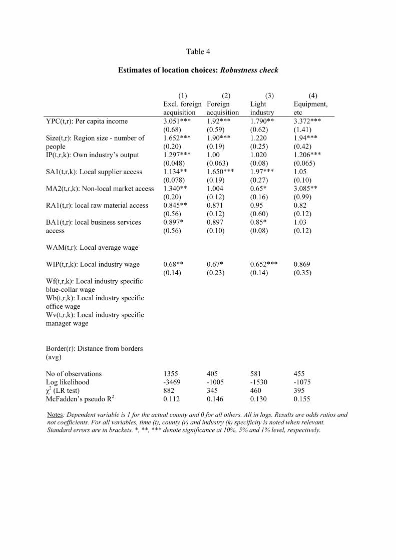
Table 4

Estimates of location choices: Robustness check

(1) (2) (3) (4) Excl. foreign

acquisition Foreign acquisition

Light industry

Equipment, etc

YPC(t,r): Per capita income 3.051*** (0.68)

1.92*** (0.59)

1.790** (0.62)

3.372*** (1.41)

Size(t,r): Region size - number of people

1.652*** (0.20)

1.90*** (0.19)

1.220 (0.25)

1.94*** (0.42)

IP(t,r,k): Own industry’s output 1.297*** (0.048)

1.00 (0.063)

1.020 (0.08)

1.206*** (0.065)

SA1(t,r,k): Local supplier access 1.134** (0.078)

1.650*** (0.19)

1.97*** (0.27)

1.05 (0.10)

MA2(t,r,k): Non-local market access 1.340** (0.20)

1.004 (0.12)

0.65* (0.16)

3.085** (0.99)

RA1(t,r): local raw material access 0.845** (0.56)

0.871 (0.12)

0.95 (0.60)

0.82 (0.12)

BA1(t,r): local business services access

0.897* (0.56)

0.897 (0.10)

0.85* (0.08)

1.03 (0.12)

WAM(t,r): Local average wage

WIP(t,r,k): Local industry wage 0.68** (0.14)

0.67* (0.23)

0.652*** (0.14)

0.869 (0.35)

Wf(t,r,k): Local industry specific blue-collar wage

Wb(t,r,k): Local industry specific office wage

Wv(t,r,k): Local industry specific manager wage

Border(r): Distance from borders (avg)

No of observations 1355 405 581 455 Log likelihood χ2 (LR test)

-3469 882

-1005 345

-1530 460

-1075 395

McFadden’s pseudo R2 0.112 0.146 0.130 0.155 Notes: Dependent variable is 1 for the actual county and 0 for all others. All in logs. Results are odds ratios and not coefficients. For all variables, time (t), county (r) and industry (k) specificity is noted when relevant. Standard errors are in brackets. *, **, *** denote significance at 10%, 5% and 1% level, respectively.