General rights Copyright and moral rights for the publications made accessible in the public portal are retained by the authors and/or other copyright owners and it is a condition of accessing publications that users recognise and abide by the legal requirements associated with these rights.

Users may download and print one copy of any publication from the public portal for the purpose of private study or research.

You may not further distribute the material or use it for any profit-making activity or commercial gain

You may freely distribute the URL identifying the publication in the public portal If you believe that this document breaches copyright please contact us providing details, and we will remove access to the work immediately and investigate your claim.

Downloaded from orbit.dtu.dk on: May 18, 2020

Locating replenishment stations for electric vehicles: Application to Danish traffic data

Wen, Min; Laporte, Gilbert; Madsen, Oli B.G. ; Nørrelund, Anders Vedsted; Olsen, Allan

Publication date:2012

Document VersionEarly version, also known as pre-print

Link back to DTU Orbit

Citation (APA):Wen, M., Laporte, G., Madsen, O. B. G., Nørrelund, A. V., & Olsen, A. (2012). Locating replenishment stationsfor electric vehicles: Application to Danish traffic data.

Locating Replenishment Stations for ElectricVehicles: Application to Danish Traffic Data

Min Wen1, Gilbert Laporte2, Oli B.G. Madsen1, Anders V. Nørrelund1 and Allan Olsen1

January 17, 2012

1Department of Transport, Technical University of Denmark, Bygningstorvet 116Vest, DK-2800 Kongens Lyngby, Denmark, {mw@transport.dtu.dk,ogm@transport.dtu.dk, ann@transport.dtu.dk, aol@transport.dtu.dk }

2 Canada Research Chair in Distribution Management and CIRRELT, HECMontréal, 3000 chemin de la Côte-Sainte-Catherine, Montréal, Canada H3T 2A7,gilbert.laporte@cirrelt.ca

Abstract

Environment-friendly electric vehicles have gained substantial attentionin governments, industry and universities. The deployment of a network ofrecharging stations is essential given their limited travel range. This paperconsiders the problem of locating electronic replenishment stations for electricvehicles on a traffic network with flow-based demand. The objective is tooptimize the network performance, for example to maximize the flow coveredby a prefixed number of stations, or to minimize the number of stations neededto cover traffic flows. Two mixed integer linear programming formulations areproposed to model the problem. These models are tested on real-life trafficdata collected in Denmark. Computational results are presented.

1 Introduction

During the past few decades, environmental concerns have generated a renewedinterest in electrical vehicles. The current yearly worldwide sales of fully electricvehicles now stand at around 20,000 units. The market is expected to grow to750,000 units in 2020 in the European Union (EU) alone (Philippe (2011)). The

1

major advantage of electrical vehicles is that they are more environment-friendlythan traditional vehicles. They emit much less CO2 and almost no air pollutants.However, electrical vehicles have a limited driving range due to the low density oftheir batteries. It is therefore important to supply electrical vehicles with rechargingstations to lengthen their autonomy. Around 1000 electric charging stations arenow in operation in the USA, distributed in 39 states (U.S. Department of Energy(2011)). It is predicted that the number of public charging points in the EU will growto close to two million by 2017 (Pike Research (2011)). In Europe, the approximateinvestment in such infrastructure over the next seven years is likely to be about fivebillion Euros (Pike Research (2011)). This expenditure will largely be motivatedby local government initiatives aimed at boosting the expansion of public charginginfrastructures for electric vehicles. It is estimated that more than 4.7 million electricvehicle charge points will be installed worldwide by 2015 (Pike Research (2011)).

Locating stations is a central issue in the deployment of charging infrastructure.In this work, we investigate the problem of locating electronic replenishment stationsfor electric vehicles on the basis of traffic flows. Two models will be developed andcompared. In the first one, the aim is to maximize the total flow captured by agiven number of stations. In the second model the aim is to minimize the numberof stations required to capture the entire flow. In both cases we impose a drivingrange constraint which ensures that every stretch of at least r km is covered by atleast one station. The problem belongs to the family of Flow Interception FacilityLocation Problems (FIFLPs) in which demand is expressed by origin-destination(OD) flows on a directed network. It is assumed that drivers can always replenishat their origin or at their destination. This means that replenishment is not an issueon OD paths not exceeding r km.

The FIFLP was introduced by Hodgson (1981) in relation with the location ofdaycare facilities. Over the past 30 years, different models have been proposed tocharacterize a wide range of applications, such as the location of police inspectionstations (Hodgson et al. (1996), Gendreau et al. (2000) and Selmić et al. (2010)),of road detecting sensors (Liu and Danczyk (2009)), of gas and refueling stations(Kuby et al. (2009), Lim and Kuby (2010), Upchurch et al. (2009), Wang and Lin(2009) and Wang and Wang (2010)), and so on. Boccia et al. (2009) provide areview on the problems, models and methods for FIFLPs.

The main contribution of this paper is the development of two models for theElectronic Replenishment Station Location Problem (ERSLP) and their assessmenton real-life traffic data collected in Denmark. The remainder of the paper is or-ganized as follows. A formal problem description and two mathematical models

2

are provided in Section 2. The data and a data preprocessing algorithm and thecomputational results are presented in Section 3, followed by conclusions in Section4.

2 Formal problem description and mathematical mod-

els

A natual way to model the ERSLP is to use a flow capturing formulation. However,as rightly noted by Lim and Kuby (2010), the ERSLP is not a standard FIFPLbecause several facilities may be required to cover a flow. Several formulationsare possible, depending on how the variables and constraints are defined. Limand Kuby (2010) have developed a model which requires the enumeration of allfacility combinations. Here we develop a more parsimonious but equivalent modelapplicable to relatively large scale applications. Our model works with a directedgraph G = (V,A), where V is a set of nodes and A = {(i, j) : i, j ∈ V, i 6= j} isa set of arcs. A node can represent the origin or the destination of an OD path orpotential location sites for stations. The set of OD paths is denoted by P . Let fp bethe traffic flow of path p. Each path p ∈ P is represented by an ordered sequence ofnodes V p = (vp1, ..., v

pl ). Different paths can share some nodes. The set of all nodes

is V = V 1∪ ...∪V |P |. We denote by tij the length of a shortest path from i to j. Thedriving range of a vehicle is the maximal distance it can drive without replenishingand is denoted by r. We denote by Sip the maximal ordered subset {i, ..., h} of asubpath p, starting at node i, that can be driven without replenishment, i.e., suchthat tih ≤ r.

2.1 Maximal flow capture model

In the maximal flow capture model (MFCM), the aim is to maximize the capturedflow using m stations, subject to the driving range constraint. This model usesbinary variables yj equal to 1 if and only if a station is located at node j, binaryvariables zp equal to 1 if and only if the flow of OD path p is covered by sufficientnumber of stations. To reduce the size of the models, we only consider those ODpaths whose length exceeds r and undominated paths: path p dominates path p′ ifV p′ ⊆ V p. Let P ′ be the resulting set of paths. The MFCM is as follows:

3

MFCM:

maximize∑p∈P ′

fpzp (1)

such that∑j∈V

yj = m (2)∑j∈Sip

yj ≥ zp ∀p ∈ P ′, i ∈ V p (3)

yj ∈ {0, 1} ∀j ∈ V (4)

zp ∈ {0, 1} ∀p ∈ P ′. (5)

In this formulation, the objective maximizes the traffic covered by the stations.Constraints (2) impose the location of m stations. They ensure that no feasiblesolution is excluded since all locations in V are considered as candidates. Constraints(3) state that every subpath of an OD path p that is covered (i.e. zp = 1) containsa replenishment station within r units of each of its nodes. Constraints (4) and (5)define the binary variables.

2.2 Total flow capture model

In the total flow capture model (TFCM), the aim is to cover all traffic with the leastnumber of stations. The model is

TFCM:

minimize∑j∈V

yj (6)

such that∑j∈Sip

yj ≥ 1 ∀p ∈ P ′, i ∈ V p (7)

yj ∈ {0, 1} ∀j ∈ V. (8)

In this model, constraints (7) ensure that each OD path is covered by at leastone station and that the driving range constraints are satisfied.

3 Computational results

Solving MFCM or TFCM requires traffic data. In Denmark which serves as a basisfor this study, such data are provided by the government which conducts trafficsurveys every 10 years. These surveys include Daily Trip Schedules which describe

4

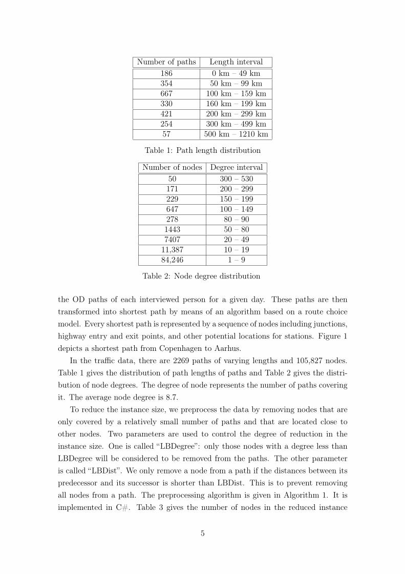
Number of paths Length interval186 0 km – 49 km354 50 km – 99 km667 100 km – 159 km330 160 km – 199 km421 200 km – 299 km254 300 km – 499 km57 500 km – 1210 km

Table 1: Path length distribution

Number of nodes Degree interval50 300 – 530171 200 – 299229 150 – 199647 100 – 149278 80 – 901443 50 – 807407 20 – 4911,387 10 – 1984,246 1 – 9

Table 2: Node degree distribution

the OD paths of each interviewed person for a given day. These paths are thentransformed into shortest path by means of an algorithm based on a route choicemodel. Every shortest path is represented by a sequence of nodes including junctions,highway entry and exit points, and other potential locations for stations. Figure 1depicts a shortest path from Copenhagen to Aarhus.

In the traffic data, there are 2269 paths of varying lengths and 105,827 nodes.Table 1 gives the distribution of path lengths of paths and Table 2 gives the distri-bution of node degrees. The degree of node represents the number of paths coveringit. The average node degree is 8.7.

To reduce the instance size, we preprocess the data by removing nodes that areonly covered by a relatively small number of paths and that are located close toother nodes. Two parameters are used to control the degree of reduction in theinstance size. One is called “LBDegree”: only those nodes with a degree less thanLBDegree will be considered to be removed from the paths. The other parameteris called “LBDist”. We only remove a node from a path if the distances between itspredecessor and its successor is shorter than LBDist. This is to prevent removingall nodes from a path. The preprocessing algorithm is given in Algorithm 1. It isimplemented in C#. Table 3 gives the number of nodes in the reduced instance

5

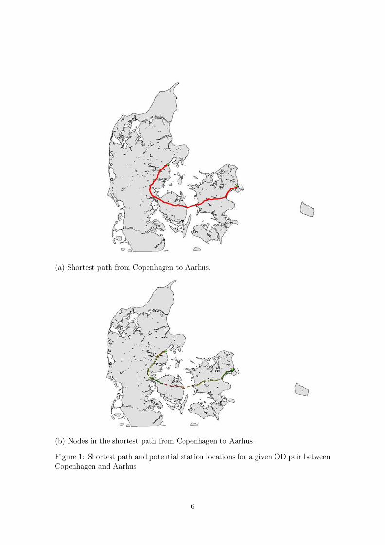
(a) Shortest path from Copenhagen to Aarhus.

(b) Nodes in the shortest path from Copenhagen to Aarhus.

Figure 1: Shortest path and potential station locations for a given OD pair betweenCopenhagen and Aarhus

6

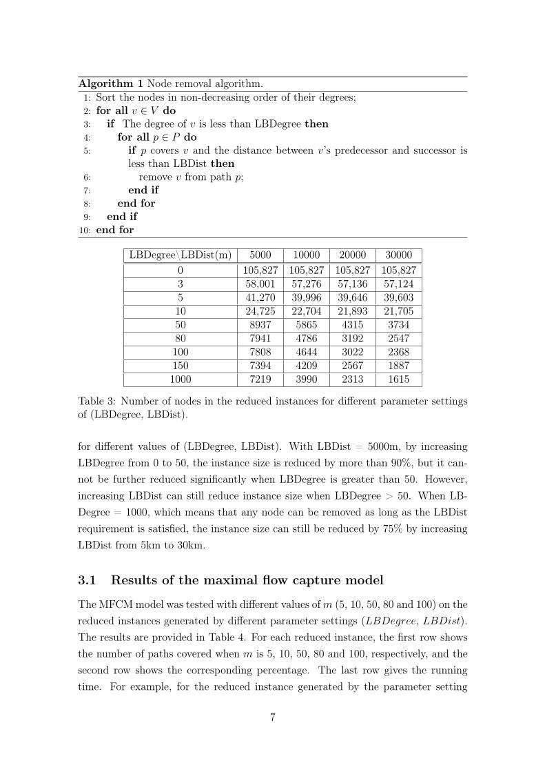
Algorithm 1 Node removal algorithm.1: Sort the nodes in non-decreasing order of their degrees;2: for all v ∈ V do3: if The degree of v is less than LBDegree then4: for all p ∈ P do5: if p covers v and the distance between v’s predecessor and successor is

less than LBDist then6: remove v from path p;7: end if8: end for9: end if

10: end for

LBDegree\LBDist(m) 5000 10000 20000 300000 105,827 105,827 105,827 105,8273 58,001 57,276 57,136 57,1245 41,270 39,996 39,646 39,60310 24,725 22,704 21,893 21,70550 8937 5865 4315 373480 7941 4786 3192 2547100 7808 4644 3022 2368150 7394 4209 2567 18871000 7219 3990 2313 1615

Table 3: Number of nodes in the reduced instances for different parameter settingsof (LBDegree, LBDist).

for different values of (LBDegree, LBDist). With LBDist = 5000m, by increasingLBDegree from 0 to 50, the instance size is reduced by more than 90%, but it can-not be further reduced significantly when LBDegree is greater than 50. However,increasing LBDist can still reduce instance size when LBDegree > 50. When LB-Degree = 1000, which means that any node can be removed as long as the LBDistrequirement is satisfied, the instance size can still be reduced by 75% by increasingLBDist from 5km to 30km.

3.1 Results of the maximal flow capture model

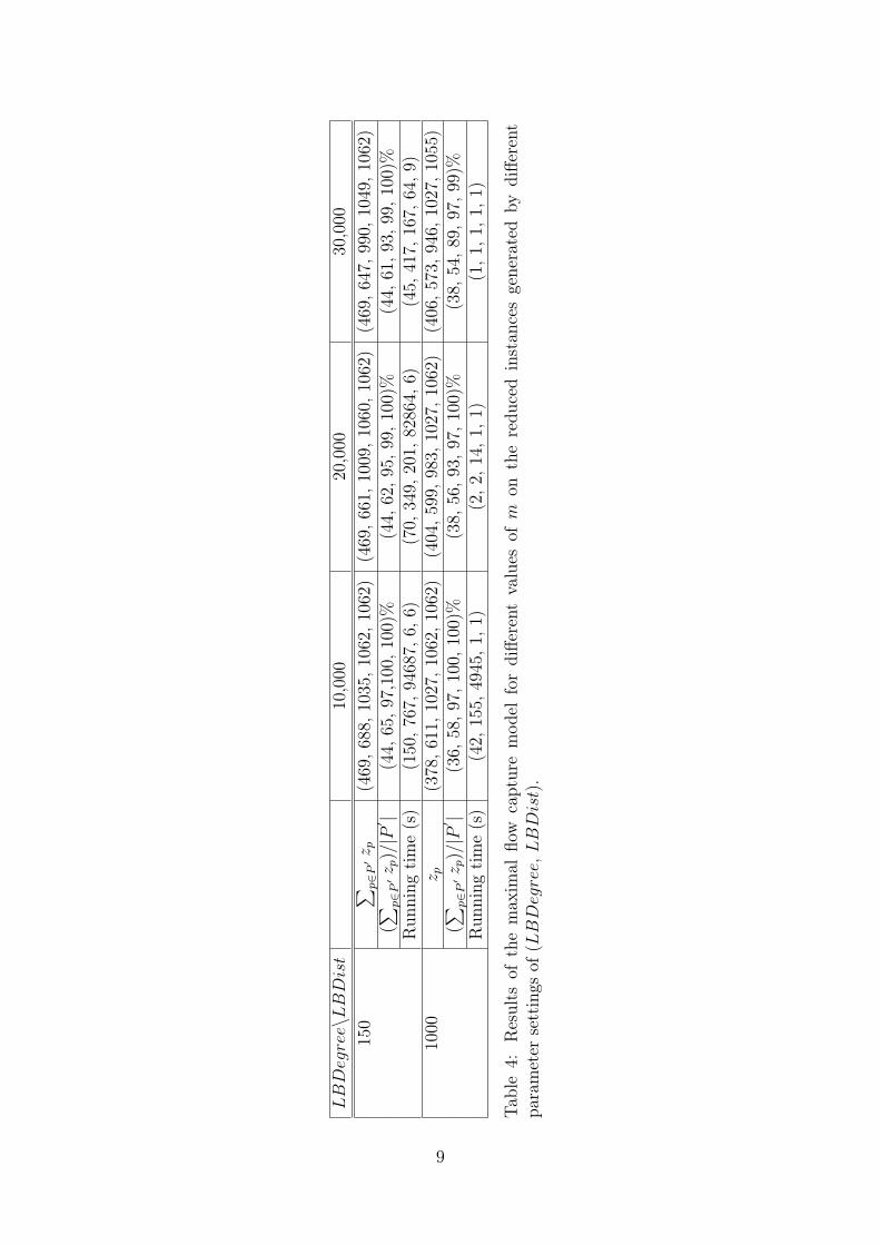
The MFCMmodel was tested with different values ofm (5, 10, 50, 80 and 100) on thereduced instances generated by different parameter settings (LBDegree, LBDist).The results are provided in Table 4. For each reduced instance, the first row showsthe number of paths covered when m is 5, 10, 50, 80 and 100, respectively, and thesecond row shows the corresponding percentage. The last row gives the runningtime. For example, for the reduced instance generated by the parameter setting

7

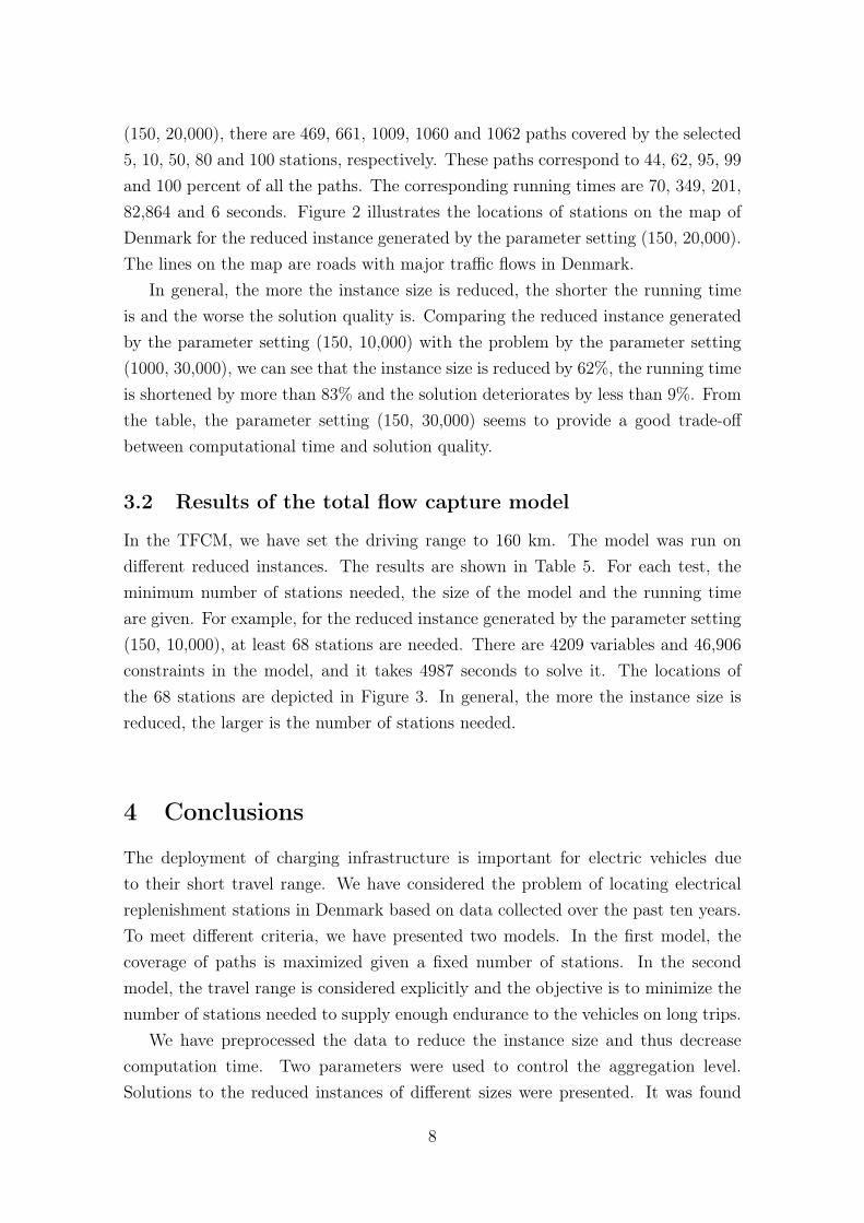
(150, 20,000), there are 469, 661, 1009, 1060 and 1062 paths covered by the selected5, 10, 50, 80 and 100 stations, respectively. These paths correspond to 44, 62, 95, 99and 100 percent of all the paths. The corresponding running times are 70, 349, 201,82,864 and 6 seconds. Figure 2 illustrates the locations of stations on the map ofDenmark for the reduced instance generated by the parameter setting (150, 20,000).The lines on the map are roads with major traffic flows in Denmark.

In general, the more the instance size is reduced, the shorter the running timeis and the worse the solution quality is. Comparing the reduced instance generatedby the parameter setting (150, 10,000) with the problem by the parameter setting(1000, 30,000), we can see that the instance size is reduced by 62%, the running timeis shortened by more than 83% and the solution deteriorates by less than 9%. Fromthe table, the parameter setting (150, 30,000) seems to provide a good trade-offbetween computational time and solution quality.

3.2 Results of the total flow capture model

In the TFCM, we have set the driving range to 160 km. The model was run ondifferent reduced instances. The results are shown in Table 5. For each test, theminimum number of stations needed, the size of the model and the running timeare given. For example, for the reduced instance generated by the parameter setting(150, 10,000), at least 68 stations are needed. There are 4209 variables and 46,906constraints in the model, and it takes 4987 seconds to solve it. The locations ofthe 68 stations are depicted in Figure 3. In general, the more the instance size isreduced, the larger is the number of stations needed.

4 Conclusions

The deployment of charging infrastructure is important for electric vehicles dueto their short travel range. We have considered the problem of locating electricalreplenishment stations in Denmark based on data collected over the past ten years.To meet different criteria, we have presented two models. In the first model, thecoverage of paths is maximized given a fixed number of stations. In the secondmodel, the travel range is considered explicitly and the objective is to minimize thenumber of stations needed to supply enough endurance to the vehicles on long trips.

We have preprocessed the data to reduce the instance size and thus decreasecomputation time. Two parameters were used to control the aggregation level.Solutions to the reduced instances of different sizes were presented. It was found

8

LBDegree\LBDist

10,000

20,000

30,000

150

∑ p∈P

′z p

(469

,688

,103

5,10

62,1

062)

(469

,661

,100

9,10

60,1

062)

(469

,647

,990

,104

9,10

62)

(∑ p∈P

′z p)/|P

′ |(44,

65,9

7,10

0,10

0)%

(44,

62,9

5,99

,100

)%(44,

61,9

3,99

,100

)%Run

ning

time(s)

(150

,767

,946

87,6

,6)

(70,

349,

201,

8286

4,6)

(45,

417,

167,

64,9

)10

00z p

(378

,611

,102

7,10

62,1

062)

(404

,599

,983

,102

7,10

62)

(406

,573

,946

,102

7,10

55)

(∑ p∈P

′z p)/|P

′ |(36,

58,9

7,10

0,10

0)%

(38,

56,9

3,97

,100

)%(38,

54,8

9,97

,99)%

Run

ning

time(s)

(42,

155,

4945

,1,1

)(2,2

,14,

1,1)

(1,1

,1,1

,1)

Table4:

Results

ofthemax

imal

flow

capturemod

elfordiffe

rent

values

ofm

ontheredu

ced

instan

cesgenerated

bydiffe

rent

parameter

settings

of(L

BDegree,

LBDist).

9

Figure 2: The locations of the stations form = 5, 10, 50, 80 and 100 in the solution tothe reduced instance generated by the parameter setting (LBDegree = 150, LBDist= 20,000).

10

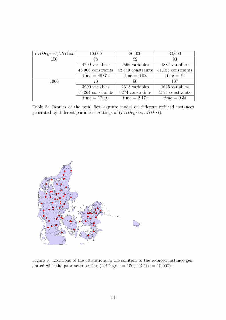
LBDegree\LBDist 10,000 20,000 30,000150 68 82 93

4209 variables 2566 variables 1887 variables46,906 constraints 42,449 constraints 41,055 constraints

time = 4987s time = 640s time = 7s1000 70 90 107

3990 variables 2313 variables 1615 variables16,264 constraints 8274 constraints 5521 constraints

time = 1700s time = 2.17s time = 0.3s

Table 5: Results of the total flow capture model on different reduced instancesgenerated by different parameter settings of (LBDegree, LBDist).

Figure 3: Locations of the 68 stations in the solution to the reduced instance gen-erated with the parameter setting (LBDegree = 150, LBDist = 10,000).

11

that the more the instance size is reduced, the larger is the number of stationsneeded and 68 stations are sufficient to ensure the driving range for the long paths.

In the future, more accurate models consisting of more real-life constraints andobjectives can be investigated. Fast metaheuristic, e.g., adaptive large neighbour-hood search, can also be developed to solve large scale problems.

Acknowledgements

This work was partly supported by the Canadian Natural Sciences and EngineeringResearch Council under grants 227837-04 and 39682-10. This support is gratefullyacknowledged.

References

Boccia, M., Sforza, A., and Sterle, C. (2009). Flow intercepting facility location:Problems, models and heuristics. Journal of Mathematical Modelling and Algo-rithms, 8(1):35–79.

Gendreau, M., Laporte, G., and Parent, I. (2000). Heuristics for the location ofinspection stations on a network. Naval Research Logistics, 47(4):287–303.

Hodgson, M, J. (1981). The location of public facilities intermediate to the journeyto work. European Journal of Operational Research, 6(2):199–204.

Hodgson, M, J., Rosing, K, E., and Zhang, J, J. (1996). Locating vehicle inspectionstations to protect a transportation network. Geographical Analysis, 28(4):299–314.

Kuby, M., Lines, L., Schultz, R., Xie, Z., Kim, J.-G., and Lim, S. (2009). Optimiza-tion of hydrogen stations in Florida using the Flow-Refueling Location Model.International Journal of Hydrogen Energy, 34(15):6045–6064.

Lim, S. and Kuby, M. (2010). Heuristic algorithms for siting alternative-fuel sta-tions using the Flow-Refueling Location Model. European Journal of OperationalResearch, 204(1):51–61.

Liu, H, X. and Danczyk, A. (2009). Optimal sensor location for freeway bottleneckidentification. Computer-Aided Civil and Infrastructure Engineering, 24(8):535–550.

12

Philippe, J. (2011). European policy on electric vehicles. Conference on Electricvehicles - Challenges of the New Mobility, Sofia.

Pike Research (2011). Strategic technology and market analysis of electric vehiclecharging infrastructure in Europe. http://www.reportlinker.com/p0503640/Strategic-Technology-and-Market-Analysis-of-Electric-Vehicle-Charging-Infrastructure-in-Europe.pdf.

Selmić, M., Teodorović, D., and Vukadinović, K. (2010). Locating inspection facil-ities in traffic networks: an artificial intelligence approach. Transportation Plan-ning and Technology, 33(6):481–493.

Upchurch, C., Kuby, M., and Lim, S. (2009). A model for location of capacitatedalternative-fuel stations. Geographical Analysis, 41(1):85–106.

U.S. Department of Energy (2011). Alternative fueling station total counts by stateand fuel type. http://www.afdc.energy.gov/afdc/fuels/stations_counts.html.

Wang, Y.-W. and Lin, C.-C. (2009). Locating road-vehicle refueling stations. Trans-portation Research Part E - Logistics and Transportation Review, 45(5):821–829.

Wang, Y.-W. and Wang, C.-R. (2010). Locating passenger vehicle refueling stations.Transportation Research Part E - Logistics and Transportation Review, 46(5):791–801.

13