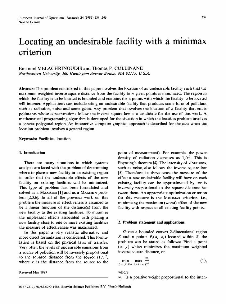
European Journal of Operational Research 24 (1986) 239-246

239North-Holland

Locating an undesirable facility with a minimax

criterion

Emanuel MELACHRINOUDIS and Thomas P . CULLINANENortheastern University, 360 Huntington Avenue-Boston, MA 02115, US .A .

Abstract: The problem considered in this paper involves the location of an undesirable facility such that themaximum weighted inverse square distance from the facility to n given points is minimized . The region inwhich the facility is to be located is bounded and contains the n points with which the facility to be locatedwill interact. Applications can include siting an undesirable facility that produces some form of pollutantsuch as radiation, noise and some gases . Any problem that involves the location of a facility that emitspollutants whose concentrations follow the inverse square law is a candidate for the use of this work . Amathematical programming algorithm is developed for the situation in which the location problem involvesa convex polygonal region. An interactive computer graphics approach is described for the case when thelocation problem involves a general region.

Keywords: Facilities, location

1. Introduction

There are many situations in which systemsanalysts are faced with the problem of determiningwhere to place a new facility in an existing regionin order that the undesirable effects of the newfacility on existing facilities will be minimized .This type of problem has been formulated andsolved as a MAXISUM [1] and as a MAXIMIN prob-lem [2,3,6]. In all of the previous work on thisproblem the measure of effectiveness is assumed tobe a linear function of the distance(s) from thenew facility to the existing facilities . To minimizethe unpleasant effects associated with placing anew facility close to one or more existing facilitiesthe measure of effectiveness was maximized .

In this paper a very realistic alternative andmore direct formulation is considered . This formu-lation is based on the physical laws of transfer .Very often the levels of undesirable emissions froma source of pollution will be inversely proportionalto the squared distance from the source (1/r2,where r is the distance from the source to the

Received May 1985

0377-2217/86/$3 .50 0 1986, Elsevier Science Publishers B .V. (North-Holland)

point of measurement) . For example, the powerdensity of radiation decreases as 1/r2 . This isPoynting's theorem [4] . The intensity of vibrations,such as noise, also follows the inverse square law[5]. Therefore, in these cases the measure of theeffect a new undesirable facility will have on eachexisting facility can be approximated by, or isinversely proportional to the square distance be-tween them. An appropriate optimization criterionfor this measure is the MINIMAx criterion, i .e .,minimizing the maximum (worst) effect of the newfacility with respect to all existing facility points.

2. Problem statement and applications

Given a bounded convex 2-dimensional regionS and n points P,(a„ b,) located within S, theproblem can be stated as follows : Find a point(x, y) which minimizes the maximum weightedinverse square distance, or

w;mm maxrr(x, y)CS 1<;<~1

wherew, is a positive weight proportional to the inten-

240

sity of the source and the susceptibility orsensitivity of the ith receiving point, and

r,2 is the square Euclidean distance between theith point and (x, y), i .e ., r, 2 = (x - a,) 2+(y-b;) 2 .

The following applications can be considered inassociation with (1) :- Selecting the best or least threatening location

for a piece of equipment or process which emitscontaminants (i .e ., dust, smoke, gas, fumes) orcreates stresses (i.e ., vibration, noise, heat) orhazards (i .e ., radiant energy) to nearby workers .

- Locating a hazardous material dump .- Locating a potentially dangerous or undesirable

facility such as a plant that has very noisyprocesses .

3. Model formulation and development

The minimax problem defined in (1) can bewritten in an equivalent form by introducing anew variable z for the objective function as fol-lows :

i=1,2,

,n .

The fact that the region S is bounded impliesthat r, 2 is also bounded and therefore z > 0 due to(2). Also the above formulation implies that z isfinite for all points (x, y) E S except for (x, y) =P„ i = 1, 2, . . ., n . Therefore a finite positive valueexists which minimizes the objective function z .

For a convex region S that has one or morenonlinear sides it is possible to approximate eachside by a sequence of linear segments . Such anapproximation is usually most satisfactory for ac-tual location problems. When the sides of theconvex polygon S are adjusted to be linear seg-ments, implementation of a mathematical pro-gramming algorithm and a computer code can beachieved . Consider a convex polygonal region de-fined by a clockwise sequence of m vertices Q,,j = 1, 2, . . ., m, or equivalently by the intersection

h'. Melachrinoudis, T.P. Cullinane / Locating facility with minimax criterion

of m linear inequalities (5) . The MINIMAX problemwith inverse square distances can then be for-mulated as follows :

The convex polygonal region S defined by (5)becomes in a 3-dimensional space a prismatic re-gion generated by the sides of S in the direction ofthe z-axis

h ;(x,Y)=c,1x+c,,2Y+cjz=0, j=1,2, . . .,m .

(6)

The constraints (4) define regions above surfacesrepresented by the boundary equations

g' (x, Y, z)= -z[(x-a,)2+(y-b,)2] +w,=0,

i=1,2, . . ., n,

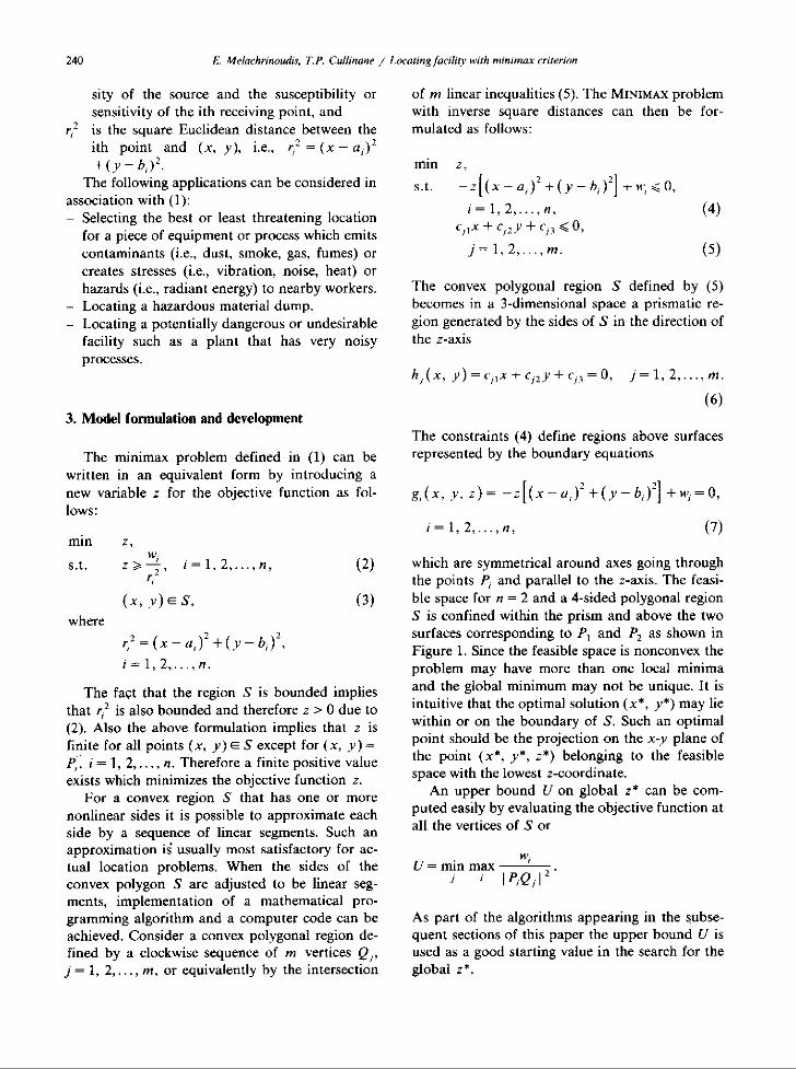
which are symmetrical around axes going throughthe points P, and parallel to the z-axis . The feasi-ble space for n = 2 and a 4-sided polygonal regionS is confined within the prism and above the twosurfaces corresponding to P, and P 2 as shown inFigure 1 . Since the feasible space is nonconvex theproblem may have more than one local minimaand the global minimum may not be unique . It isintuitive that the optimal solution (x*, y*) may liewithin or on the boundary of S. Such an optimalpoint should be the projection on the x-y plane ofthe point (x*, y*, z*) belonging to the feasiblespace with the lowest z-coordinate .

An upper bound U on global z* can be com-puted easily by evaluating the objective function atall the vertices of S or

w,U = min max

I PQ1 1 2

(7)

As part of the algorithms appearing in the subse-quent sections of this paper the upper bound U isused as a good starting value in the search for theglobal z* .

mins .t .

z,Z ,

w;z, i=1,2, . . .,n, (2)g

(3)(x, y) ES,

where

r2=(x-a,)'+(y-

mins .t .

z,-z[(x-a,)r+(y-b,)21 +%t; 0,

i=1, 2, . . .,n, (4)c 1,x+C, 2y+C 3 1<0,

j=1, 2, . . .,m . (5)

E. bfelachrinoudis, T. P. Cullinane / nearing fact//tv with minimax criterion

4. Solution method for a convex polygon S

4.1 . Properties of local minima

The local minima of problem (1) satisfy thefollowing three properties .

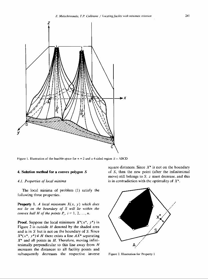
Property 1. A local minimum X(x, y) which doesnot lie on the boundary of S will lie within theconvex hull H of the points P;, i = 1, 2, . . ., n .

Proof. Suppose the local minimum X*(x*, y*) inFigure 2 is outside H denoted by the shaded areaand is in S but is not on the boundary of S. SinceX*(x*, y*) (4 H there exists a line AX* separatingX* and all points in H, Therefore, moving infini-tesimally perpendicular to this line away from Hincreases the distances to all facility points andsubsequently decreases the respective inverse

Figure 1 . Illustration of the feasible space for n = 2 and a 4-sided region S = ABCD

Figure 2 . Illustration for Property l

24 1

square distances . Since X* is not on the boundaryof S, then the new point (after the infinitesimalmove) still belongs to S. z must decrease, and thisis in contradiction with the optimality of X* .

242

E. Melachrinoudis, T P. Cullinane / Locating facility with minimax criterion

Property 2. At a local minimum within H at leastthree constraints of type (2) are binding .

Proof . Assume X*(x*, y*) is in the interior of Hand (x*, y*, z*) represents a local minimum . Itfollows that

wz* > r**i for all i,

where

r*F=(x*-a;)'+(y*-b,)z .

Now, we examine the plane z = z* . Consider thefollowing three cases :

1 . z* > r*zZ for all facilities i .

Clearly, the point (x*, y*, z* -A) is feasible forsmall enough d, so (x*, y*, z*) is. not locallyoptimal .

II .w;

z* > r* z

Z* Wk

r* 2k

for all facilities i except k and

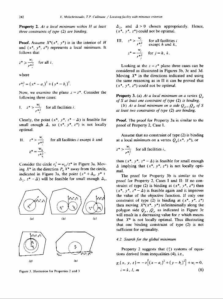
Consider the circle r, = wA/z* in Figure 3a . Mov-ing X* in the direction P,, X* away from the circle,indicated in Figure 3a, the point (x* +,A,, y* +A z , z* - A) will be feasible for small enough d,

(a)

(d)

(b)

(e)

Figure 3 . Illustration for Properties 2 and 3

(c)

A2, and d > 0 chosen appropriately . Hence,(x*, y*, z*)could not be optimal .

wIII . z* > =

for all facilities ir*2

except h and k,W;z* _W; for j=h, k .

>

Looking at the z = z* plane three cases can beconsidered as illustrated in Figures 3b, 3c and 3d .Moving X* in the directions indicated and usingthe same reasoning as in II it can be proved that(x*, y*, z*) could not be optimal .

Property 3. (a) At a local minimum on a vertex Q eof S at least one constraint of type (2) is binding .

(b) At a local minimum on a side Q,,,,Qe of Sat least two constraints of type (2) are binding.

Proof. The proof for Property 3a is similar to theproof of Property 2, Case I .

Assume that no constraint of type (2) is bindingat a local minimum on a vertex Qa(x*, y*), or

z* >W- for all facilities i,r* z

then (x*, y*, z* -d) is feasible for small enoughd implying that (x*, y*, z*) is not locally opti-mal .

The proof for Property 3b is similar to theproof for Property 2, Cases I and II : If no con-straint of type (2) is binding at (x*, y*, z*) then(x*, y*, z* -A) is feasible again and it improvesthe value of the objective function . If only oneconstraint of type (2) is binding at (x*, y*, z*)then moving X*(x*, y*) infinitesimally along thepolygon side Q,,,,Q,, as indicated in Figure 3ewill result in a decreasing value for z which meansthat X* is not locally optimal . Thus illustratingthat one binding constraint of type (2) is notsufficient for optimality .

4.2. Search for the global minimum

Property 2 suggests that ( ;) systems of equa-tions derived from inequalities (4), i .e .,

g,(x, y, z)=-z (x-a;) 2 +(y-b;)z ] +w;=0,

i=k, 1, m

(8)

E. Melaehrinoudis, T. P . Cullinane / Locating facility with minimax criterion

must be solved and tested for feasibility using theinequalities (4) and (5) . A system of equations (8)has at most two solutions (x, y, z) . Since a solu-tion corresponding to three collinear points P;,i = k, 1, m cannot yield a local minimum, onlytriples of noncollinear points P, should be consid-ered .

The resulting set of feasible solutions (x, y, z)contains the set of all local minima within Hincluding any nondegenerate local minima at whichmore than three constraints of type (2) are bind-ing. According to Properties I and 2 if the globalminimum does not lie on the boundary of S it willbe found within H by checking all feasible solu-tions (x, y, z) of the systems (8) for the lowestvalue of z .

The derivation of the upper bound U by scan-ning all vertices of S and its use in the subsequentalgorithm guarantees to find the global minimumif it appears on a vertex . Therefore, a search forlocal minima on the vertices of S according toProperty 3a can be avoided .

Property 3h suggests that ( ;) systems of equa-

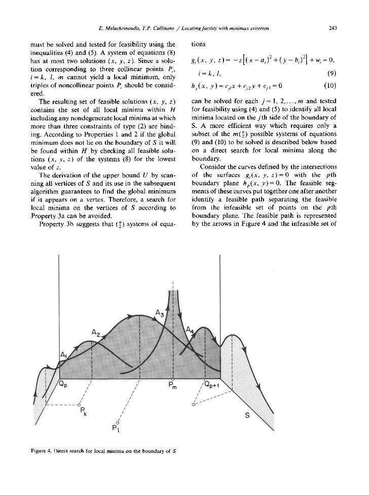
Figure 4. Direct search for local minima on the boundary of S

lions

g' (x, y, z)=-z[(x-a,)2+(y-b,)2]+w;=0,

i=k, 1,

(9)

ht (x, y)=c,,x+c,ay+C,3=0

(10)

can be solved for each j = 1, 2, . . ., m and testedfor feasibility using (4) and (5) to identify all localminima located on the j th side of the boundary ofS. A more efficient way which requires only asubset of the m(z) possible systems of equations(9) and (10) to be solved is described below basedon a direct search for local minima along theboundary .

Consider the curves defined by the intersectionsof the surfaces g;(x, y, z) = 0 with the pthboundary plane he(x, y)=0 . The feasible seg-ments of these curves put together one after anotheridentify a feasible path separating the feasiblefrom the infeasible set of points on the pthboundary plane . The feasible path is representedby the arrows in Figure 4 and the infeasible set of

243

244

E. Melachrinoudis, T P. Cullinane / Locating facility with minimax criterion

Table t

n

10

20

40 60 80 100 120 140 160

Time(see) 0.031 0.212 1.53 4.72 10.4 19.3 30 .2 48.6 74.2

points by the shaded area . Only the points of thefeasible path at which the path segment changesshould be checked if they improve the value of theobjective function z, i .e ., the points A„ A 2 , A 3 ,A 4 for the pth boundary plane illustrated in Fig-ure 4 . This accounts for solving (n - 1)E; , f, sys-tems of equations (9) and (10) where f- is thenumber of feasible path segments for the f-thboundary plane,

4.3. Algorithm AI for a convex polygons S

The following algorithm starts with a solutioncorresponding to the upper bound U on global z*and it improves that solution by performing first asearch for the global minimum within H andsecond a direct search along the boundary of S.1 . Start with the upper bound U on global z* .

Denote by (x*, y*, z*) the corresponding solu-tion .

2. Take a new combination of three noncollinearpoints ft, i = k, 1, m . If a new combination ofpoints cannot be selected go to 3 . Solve thesystem of the corresponding equationsg, (x, y, z) =0, i=k, l, m . Check each solu-tion (x, y, z) whether it is feasible and whetherz < z*; then (x*, y*, z*) F (x, y, z). RepeatStep 2 .

3. Take the first vertex Q, of the boundary of S .Then (x, y) F Q„ p - 1 . Find the point P„for which the surface g, (x, y, z)=0 identifiesthe first feasible path segment at Q 1 :

Wk

W'max

r*2

I<, ~n \ r,` ,

4. If p > m stop . Otherwise, go to Step 5 .

fable 2

10

is

20

Au

Figure 5 . Example problem

5 . Move along the feasible path of the intersectionof the pth boundary plane hr(x, y) = 0 withthe surface g, (x, y, z) = 0 clockwise fromvertex Qt, to Q,, until either another surfaceis encountered denoted by i = I or the nextplane p + I as shown in Figure 4. Denote theintersection point by (x, y, z). If (x, y) = Qp+1then p .- p + 1 and go to Step 4. Otherwise, ifz < z* then (x*, y*, z*)F (x, y, z), k -1 andrepeat Step 5 .

4.4. Computational experience

The computational complexity of the algorithmis O(n 4 ) since (3) combinations of the points areconsidered in Step 2 of the algorithm and each oneof them is tested for feasibility using (n - 1) com-parisons . The storage area is O(n) is complexity .

Several problems were created by generatingpoints within a rectangular region S using theuniform distribution. The weights were also as-signed at random between I and 5. The run timeson a VAX-11/780 in Table 1 show that on theaverage the time is increasing with a power of napproximately equal to 2 .9 .

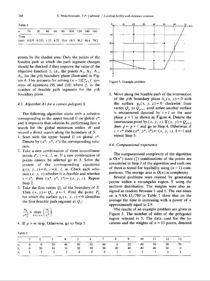
The results of an example problem are given inFigure 5 . The number of sides of the polygonalregion selected is 5 . The data used for the lo-cations and the weights of n = 13 points, denoted

1 1 2 3 4 5 6 7 8 9 10 11 12 13

11 ; 0 0 20 40 50 20 40 0 20 40 50 30 70h, 0 20 10 10 20 30 30 40 40 40 40 50 0

1 2 2 2 4 4 4 1 1 1 1 2 1

min

,

s.t .

ri >_

i=1,2 . .

(x, y) G S .

E. Mefachrinoudis, T.P. Cullinane / Locaiing/acilitr with mininmx criterion

245

by * in Figure 5, are given in Table 2 .The global minimum found is (x, y, z) = (59 .03,

0, 0.008307), denoted by G .

5 . An interactive graphics approach to the minimaxproblem for a region of any shape

To facilitate the development of an interactivegraphics approach an equivalent formulation ofthe minimax problem given in (1) has been devel-oped .

In a very large percentage of the actual situa-tions in which the model described by equation (1)applies, the region is not convex . In some in-stances the region S may be made up of morethan one disjoint convex set. Good examples arefound in problems that involve geographical re-gions such as states, countries or islands . Thenonconvex property prevents the application ofthe algorithm developed earlier. A graphics ap-proach can be utilized to solve the nonconvexproblem .

An equivalent approach to the formulationgiven in (1) can be written as shown below sincez>0.

(11)

(12)

For a fixed value of z (11) and (12) suggest thata feasible point (x, y) should be within the

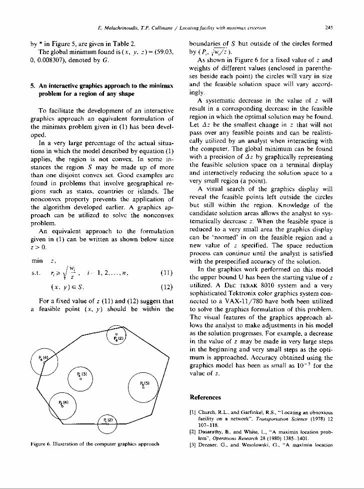
Figure 6 . Illustration of the computer graphics approach

boundaries of S but outside of the circles formedby (P;, y' w,/z ) .

As shown in Figure 6 for a fixed value of z andweights of different values (enclosed in parenthe-ses beside each point) the circles will vary in sizeand the feasible solution space will vary accord-ingly-

A systematic decrease in the value of z willresult in a corresponding decrease in the feasibleregion in which the optimal solution may he found .Let az be the smallest change in z that will notpass over any feasible points and can be realisti-cally utilized by an analyst when interacting withthe computer. The global minimum can be foundwith a precision of az by graphically representingthe feasible solution space on a terminal displayand interactively reducing the solution space to avery small region (a point) .

A visual search of the graphics display willreveal the feasible points left outside the circlesbut still within the region . Knowledge of thecandidate solution areas allows the analyst to sys-tematically decrease z. When the feasible space isreduced to a very small area the graphics displaycan be `zoomed' in on the feasible region and anew value of z specified . The space reductionprocess can continue until the analyst is satisfiedwith the prespecified accuracy of the solution .

In the graphics work performed on this modelthe upper bound U has been the starting value of zutilized . A DEC TERAK 8010 system and a verysophisticated Tektronix color graphics system con-nected to a VAX-11/780 have both been utilizedto solve the graphics formulation of this problem,The visual features of the graphics approach al-lows the analyst to make adjustments in his modelas the solution progresses . For example, a decreasein the value of z may be made in very large stepsin the beginning and very small steps as the opti-mum is approached. Accuracy obtained using thegraphics model has been as small as 10 -5 for thevalue of z .

References

[1] Church, R .L ., and Garfinkel, R.S ., "Locating an obnoxiousfacility on a network", Transportation Science (1978) 12107-118 .

(2] Dasarathy, B ., and White, L ., "A maximin location prob-lem", Operations Research 28 (1980) 1385-1401 .

[3] Drezner . G ., and Wesolowski, G., "A maximin location

246 E. Melachrinoudis, T P. Cullinane / Locating facility with minimax criterion

problem with maximum distance constraints", AIIE Trans-actions 12 (1980) 249-252 .

[4] Jordan, E.C ., and Balmain, K.G ., Electromagnetic wavesand radiating systems, Prentice-Hall, Englewood Cliffs, NJ,1979 .

[5] Lipscomb. D.M ., and Taylor, Jr., A.C ., Noise Control,Handbook of Principles and Practices, Van Norstraind Rein-hold, New York, 1978.

[6] Melachrinoudis, E., "The maximin location problem usinga Euclidean metric", Ph. D. thesis, University of Mas-sachusetts, 1980 .