1

Localization Methods for a Mobile Robot in UrbanEnvironments

Atanas Georgiev and Peter K. AllenComputer Science Department, Columbia University, New York, NY

�atanas,allen�@cs.columbia.edu

Abstract—This paper addresses the problems of designing, building and

using mobile robots for urban site modeling. It presents workon both system and algorithmic aspects. On the system level,we have designed and built a functioning autonomous mobilerobot. The design extends an existing robotic vehicle with asensor suite consisting of a digital compass with an integratedinclinometer, a global positioning unit, and a camera mounted ona pan-tilt head. The system is controlled by a distributed softwarearchitecture for mobile robot navigation and site modeling. Onthe algorithmic level, we have developed a localization systemthat employs two methods. The first method uses odometry, thecompass module and the global positioning sensor. An extendedKalman filter integrates the sensor data and keeps track of theuncertainty associated with it. The second method is based oncamera pose estimation. It is used when the uncertainty fromthe first method becomes very large. The pose estimation isdone by matching linear features in the image with a simpleand compact environmental model. We have demonstrated thefunctionality of the robot and the localization methods with real-world experiments.

Index Terms— Mobile robots, localization, computer vision

I. INTRODUCTION

There are many ways in which mobile robots can be usefuland few people doubt that the future holds an importantplace for them in our lives. They are expected to alleviate,and possibly completely take over, tedious, monotonous andpainstaking tasks. Examples include surveying, mapping, mod-eling, transportation and delivery, security, fire safety, andrecovery from disasters. Some level of autonomy is envisionedin our cars and the wheelchairs of disabled people. Yet, aftermore than three decades of research, we still do not see manyrobots scurrying about and helping us in our daily chores.

The problem of building a functional autonomous mobilerobot that can successfully and reliably interact with thereal-world is very difficult. It involves a number of issues— such as proper design, choice of sensors, methods forlocalization, navigation, planning, and others, — each of whichis a challenge on its own. The environment of operation alsoplays an important role. Much of the existing research hasbeen focused on solving these issues indoors because of itsslightly more predictable nature (e.g. flat, horizontal, well-structured, smaller scale). On the other hand, many of theinteresting applications are outdoors where fewer assumptionscan be taken for granted.

In this paper, we address the problem in outdoor urbanenvironments. These kinds of environments pose their own

unique set of challenges that differentiate them from both theindoor and the open-space outdoor landscapes. On the onehand, they are usually too large to consider applying certaintechniques that achieved success indoors. On the other hand,typical outdoor sensors, such as GPS, have problems withreception around buildings.

While we have tried to keep the methods presented here gen-eral, we have focused on the development of our mobile robotsystem with a specific application in mind. The AVENUEproject at the Columbia University Robotics Laboratory targetsthe automation of the urban site modeling process [1]. Themain goal is to build geometrically accurate and photometri-cally correct models of complex outdoor urban environments.These environments are typified by large 3-D structures thatencompass a wide range of geometric shapes and a very largescope of photometric properties.

High-quality site models are needed in a variety of appli-cations, such as city planning, urban design, fire and policeplanning, historical preservation and archaeology, virtual andaugmented reality, geographic information systems and manyothers. However, they are typically created by hand which isextremely slow and error prone. The models built are oftenincomplete and updating them can be a serious problem.AVENUE addresses these problems by building a mobilesystem that will autonomously navigate around a site andcreate a model with minimum human interaction if any.

The entire task is complex and requires the solution of anumber of fundamental problems:� In order to create a single coherent model, scans and

images of the scene taken from multiple viewpoints needto be registered and merged.

� To provide full coverage, there must be a way to tell whatpart of the scene is not yet in the model and where to goto ensure a good view of it. Better yet, it is desirable toplan the data acquisition so as to minimize the cost (suchas time, price or total travel distance).

� Given a desired acquisition location, a safe path mustbe determined that will take the sensors there from theircurrent position.

� To acquire the desired data, the sensors need to bephysically moved and accurately positioned at the targetlocations.

� The user must be able to monitor and control the processat any given stage.

The first two problems have already been successfullyaddressed by Stamos and Allen [2]. They developed a compre-

2

hensive system for the automated generation of accurate 3-Dmodels of large-scale environments using a laser range finderand a camera and provided a framework for sensor planningutilities. They demonstrated the feasibility of their approachby creating models of various buildings. Additionally, a safepath planner based on Voronoi diagrams has been developedin our group by Paul Blaer [3].

Here, we are addressing the remaining aspects of this list.We are introducing an autonomous mobile platform operatingaccording to the following scenario : Its task is to go to desiredlocations and acquire requested 3-D scans and images ofselected buildings. The locations are determined by the sensorplanning system and are used by the path planning system togenerate reliable trajectories which the robot follows. Whenthe rover arrives at the target location, it uses the sensors toacquire the scans and images and forwards them to the mod-eling system. The modeling system registers and incorporatesthe new data into the existing partial model of the site (whichin the beginning could be empty). After that, the view planningsystem decides upon the next best data acquisition locationand the above steps repeat. The process starts from a certainlocation and gradually expands the area it has covered until acomplete model of the site is obtained.

The design and implementation of our mobile platforminvolved efforts that are related and draw from a large amountof existing work. For localization, dead reckoning has alwaysbeen attractive because of its pervasiveness [4]–[6]. With therapid development of technology, GPS receivers are quicklybecoming the sensor of choice for outdoor localization [7]–[9]. Imaging sensors, such as CCD cameras and laser rangefinders, have also become very popular mobile robot compo-nents [10]–[13]. Various methods for sensor integration anduncertainty handling have been proposed [14]–[18]. A verypopular and successful idea is to exploit the duality betweenlocalization and modeling and address both issues in the sameprocess, known as SLAM – Simultaneous Localization andMap Building [16], [17], [19], [20]. Sensors and methods forindoor localization have been comprehensively reviewed intwo books [21], [22]. Another excellent book presents casestudies of successful mobile robot systems [23].

Researchers from the Australian Centre for Field Roboticshave made significant progress towards using SLAM in out-door settings. Dissanayake et al have proved that a solutionto the SLAM problem is possible and presented one suchimplementation [24]. Guivant et al have furter looked intooptimizing the computational aspects of their algorithm andhave applied it to an unstructured natural environment [25].

Chen and Shibasaki have noticed that GPS accuracy be-comes poor for navigation in many areas [26]. They haveaddressed the problem with the addition of a camera and agyro to achieve a better and more stable performance. Whiletheir work does not discuss how the sensor integration is done,it is clear that the camera and an environmental model obtainedfrom a geodetic information system (GIS) play key roles intheir method. The authors have considered situations whereGPS, GIS or both data are unavailable and have implementedboth absolute and relative to previous pose localization.

Nayak has specifically addressed localization in urban en-

Fig. 1. The mobile platform used in this work.

vironments by a sensor suite consists of four GPS antennaeand a low-cost inertial measurement unit [27]. The sensorintegration is done by an indirect Kalman filter estimating theerror of the inertial measurement unit, similar to my case.Since the sensors are mounted on a car moving at sufficientlyhigh velocities (greater than �����), he is also using thevelocity and heading readings from the GPS sensors. Testswere performed using simulated GPS outages of 20 secondduration. The resulting error in the estimate was around ��.An obvious drawback to this approach is the requirement forfour GPS receivers mounted on a relatively large platform.The resulting error, while sufficient for many applications, isnot acceptable for mobile robot navigation.

Our approach delivers a functional mobile robot systemcapable of operating accurately under the challenges of urbanenvironments. Whenever needed, we are making use of uniqueurban characteristics to facilitate the estimation of the robotlocation. Of all outdoor environments, urban areas seem topossess the most structure in the form of buildings. Thelaws of physics dictate common architectural design principlesaccording to which the horizontal and vertical directions playan essential role and parallel line features are abundant. Thesystem presented here takes advantage of these characteristics.

The rest of this paper is organized as follows: Next is asection that describes the work and considerations that wentinto the design, the architecture and the various componentsof our mobile platform. Section III describes the first of ourlocalization methods, based on odometry, a digital compassmodule and global positioning. Section IV presents our vision-based localization methods. Experimental results are shown insection V and in section VI, we conclude with a summary anda discussion on future extensions of this work.

II. SYSTEM DESIGN AND IMPLEMENTATION

The design of a mobile robot for urban site modelinginvolves a myriad of issues related to both its safe naviga-

3

tion and the necessary data acquisition. Some of the mostimportant issues are: the choice of a robotic vehicle, thechoice of sensors, the sensor placement, the software systemarchitecture, and the means of remote communication withthe robot. Ideally, all of these are considered at the designstage, before moving on to implementation. In practice, someof the design decisions are already made by virtue of existinghardware or other practical considerations. This was the casewith our mobile platform and the scanning equipment.

A. Hardware

The mobile robot we used as a test bed for this work isan ATRV-2 model manufactured by iRobot (Figure 1). It hasbuilt-in odometry and twelve sonars. It has a regular PC on-board and provides a power supply which amounts to aboutthree hours of standalone operation. Its payload of ��� �� isenough to accommodate the scanner, its electronics controllerbox, and the additional periphery we have installed. The robotcan move as fast as ���� and handle slopes of up to ��degrees. An additional benefit is that it is a holonomic vehicle,that is, it has zero turning radius.

The sensor suite on the robot has to provide sufficient data toallow for safe navigation and accurate modeling. The modelingmethod already developed dictates the use of a 3-D rangefinder and a color camera. Both are provided by a Cyrax 2500laser scanner that has a nominal accuracy of ��� and rangeof up to ����.

For successful navigation, the robot needs to be able todetect its position in the environment. An essential requirementis that the robot has an idea of its location at any given momentin time. This is best accomplished by proprioceptive sensors— ones that allow for pose computation based only on internalmeasurements of the robot motion. Odometry is typically usedas it is provided in almost every mobile robot, requires littlecomputation, and works in real-time.

To help reduce some of the error accumulation problemswith odometry and obtain a better estimate of the robotorientation, we have added a Honeywell HMR3000 digitalcompass module, which includes an integrated roll-pitch sen-sor and provides fast update rates of up to ����. Its roll-pitchaccuracy is ���Æ and its heading accuracy is better than ���Æ

(root-mean-square).An inherent limitation of proprioceptive and dead-reckoning

sensors on mobile robots is their unbounded error accumula-tion. It can only be alleviated by the addition of appropriateexteroceptive sensors – ones that make observations of therobot environment. For outdoor operation, global positioningsensors are particularly attractive, since they are explicitlydesigned for this purpose and have the necessary infrastructurealready in place. We have equipped our robot with an AshtechGG24C GPS+GLONNASS1 receiver which is accurate downto � � in real-time kinematic (RTK) mode.

The combination of dead-reckoning and GPS has beenproven very beneficial. GPS is known to exhibit an unstablehigh-frequency behavior manifested by sudden “jumps” of the

1Throughout this paper we will use GPS to designate any or both of theU.S. NAVSTAR GPS and the Russian GLONASS infrastructures.

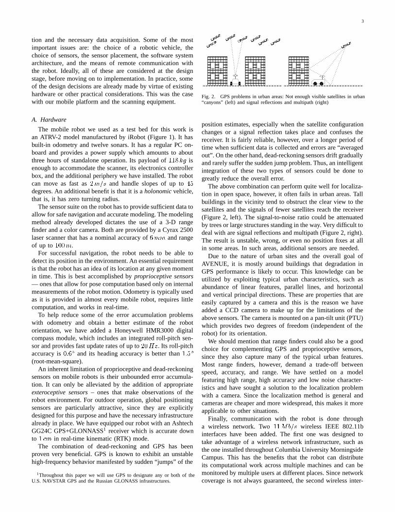
Fig. 2. GPS problems in urban areas: Not enough visible satellites in urban“canyons” (left) and signal reflections and multipath (right)

position estimates, especially when the satellite configurationchanges or a signal reflection takes place and confuses thereceiver. It is fairly reliable, however, over a longer period oftime when sufficient data is collected and errors are “averagedout”. On the other hand, dead-reckoning sensors drift graduallyand rarely suffer the sudden jump problem. Thus, an intelligentintegration of these two types of sensors could be done togreatly reduce the overall error.

The above combination can perform quite well for localiza-tion in open space, however, it often fails in urban areas. Tallbuildings in the vicinity tend to obstruct the clear view to thesatellites and the signals of fewer satellites reach the receiver(Figure 2, left). The signal-to-noise ratio could be attenuatedby trees or large structures standing in the way. Very difficult todeal with are signal reflections and multipath (Figure 2, right).The result is unstable, wrong, or even no position fixes at allin some areas. In such areas, additional sensors are needed.

Due to the nature of urban sites and the overall goal ofAVENUE, it is mostly around buildings that degradation inGPS performance is likely to occur. This knowledge can beutilized by exploiting typical urban characteristics, such asabundance of linear features, parallel lines, and horizontaland vertical principal directions. These are properties that areeasily captured by a camera and this is the reason we haveadded a CCD camera to make up for the limitations of theabove sensors. The camera is mounted on a pan-tilt unit (PTU)which provides two degrees of freedom (independent of therobot) for its orientation.

We should mention that range finders could also be a goodchoice for complementing GPS and proprioceptive sensors,since they also capture many of the typical urban features.Most range finders, however, demand a trade-off betweenspeed, accuracy, and range. We have settled on a modelfeaturing high range, high accuracy and low noise character-istics and have sought a solution to the localization problemwith a camera. Since the localization method is general andcameras are cheaper and more widespread, this makes it moreapplicable to other situations.

Finally, communication with the robot is done througha wireless network. Two ����� wireless IEEE 802.11binterfaces have been added. The first one was designed totake advantage of a wireless network infrastructure, such asthe one installed throughout Columbia University MorningsideCampus. This has the benefits that the robot can distributeits computational work across multiple machines and can bemonitored by multiple users at different places. Since networkcoverage is not always guaranteed, the second wireless inter-

4

GPS PTURobotCompassCameraScanner

Odo Drive PTU

Controller

Navigator

Localizer

AttitudeGPSImageScan

videoserver

GPSserver

attitudeserver

ATRV-2server

PTUserver

navserver

scanserver

Modeler ViewPlanner PathPlanner

UserInterface

Images,Models

AreaMaps

on-boardPC

remotehost 1

remotehost 3

remotehost 2

Fig. 3. The system architecture. Solid rectangles represent components, dotted rectangles are processes, and dashed rectangles group processes running onthe same machine. The arrows show the data flow between components

face is configured to work in an “ad hoc” mode in which itwill connect directly to a portable computer without the needfor installed network infrastructure.

B. System Architecture

Our system architecture (Figure 3) addresses a number ofimportant issues, such as flexibility and extensibility, distri-bution of computation, communication link independence, re-mote monitoring and control, and data storage and utilization.It is based on the manufacturer’s development platform [29].Its main building blocks are concurrently executing distributedsoftware components. Each component is a software abstrac-tion of a hardware device or a specific functionality. Forexample, Odo is an abstraction of the robot odometric device,Drive is an abstraction of the robot actuators, and Localizercomputes the robot pose.

Components can communicate with one another withinthe same process, across processes and even across physicalhosts. The main communication channels for data exchangeare called streams. A data stream is started by a component,called a source, which generates the data or reads it from ahardware device. Streams end with a sink — a componentwhich is the final recipient of the data and usually sends itdirectly to an actuator. Interested components can supply datato a sink or register with a source to receive updates everytime they become available. A component may also providean additional interface with a set of specific commands that itcan understand and execute.

Components performing related tasks are grouped intoservers. A server is a multi-threaded program that handlesan entire aspect of the system, such as navigation control orrobot interfacing. Each server has a well-defined interface thatallows clients to send commands, check its status or obtaindata. To ensure maximum flexibility, each hardware device is

controlled by its own server. The hardware servers are usuallysimple and serve three purposes:

1) Insulate the other components from the low-level hard-ware details, such as interface and measurement units.

2) Provide multiple, including user-defined, views of thedata coming from the device. For example, a servermay distribute its position data with respect to differentcoordinate systems.

3) Control the volume of data flow; for example, the rateat which images will be taken.

Our hardware setup is accessed and controlled by sevenservers (Figure 3, upper row of dotted triangles) that performsome or all of the tasks above. The NavServer (beneath thehardware servers) builds on top of the hardware servers andprovides a higher-level interface to the robot. A set of moreintuitive commands, such as “go there”, “establish a localcoordinate system here”, and “execute this trajectory”, arecomposed out of the low-level hardware control instructionsor data. The server also provides feedback on the progress ofthe current tasks. It consists of three components:

1) The Localizer is the part of the system that is the mainfocus of the next two sections. It reads the streamscoming from the odometry, the attitude sensor, the GPS,and the camera, registers their data with respect tothe same coordinate system, and produces an overallestimate of the robot pose and velocity according to themethods described in the following sections.

2) The Controller is a motion control component thatbrings the robot to a desired pose. It executes commandsof the type ���� and ������. Based on its target and theupdates from the Localizer, it produces pairs of desiredrotational and angular velocities and feeds them to theDrive component of the ATRV2Server.

3) The Navigator monitors the work of the Localizer andthe Controller, and handles most of the communication

5

with the remote components. It accepts commands forexecution and reports the overall progress of the mis-sion. It is optimized for network traffic: it filters outthe unimportant information coming from the low-levelcomponents and provides a compact view of the currentstate of the system.

A mission consists of commands that are carried out se-quentially. The Navigator itself does not execute most of thecommands — it simply stores them and resends them to theController, one at a time. It monitors the progress of thecurrent command and, if it completes successfully, starts thenext one. Additionally, a small group of emergency commandsexists, such as stop, pause, and resume, that are processedimmediately.

The commands stored in the Navigator are accessible toother components. This is useful in two ways. First, it allowsusers who have just connected to the robot to see what it istrying to achieve and how much it has accomplished. Second,it allows the robot to continue its mission, even if the networkconnectivity is temporarily lost. Moreover, this is the only wayto accomplish a mission that requires passing through a regionnot covered by the wireless network.

The mission command sequence is usually composed by thePath Planner which converts the target sensor acquisition poseobtained by the View Planner into a sequence of navigationand data acquisition instructions according to a 2-D mapof the area. The View Planner generates a new target afterthe Modeler updates the model with new scans and imagesreported by the ScanServer.

The computation needs to be distributed because of theheavy requirements of the modeling application. The under-lying framework and the wireless network interface make itpossible for a server to run on a computer not physicallyresiding on the robot or for a client (such as the user interface)to connect and monitor the status of each component. The stan-dardized way of communication between components makesthe architecture very flexible in that various functionalitiescan be achieved by simply adding or replacing an existingcomponent with a new one. For example, when we want totest a particular behavior of the control system indoors (whereGPS data, of course, is not available), all we need to do is runa program GPSSimulator instead of the GPSServer.

C. User Interface

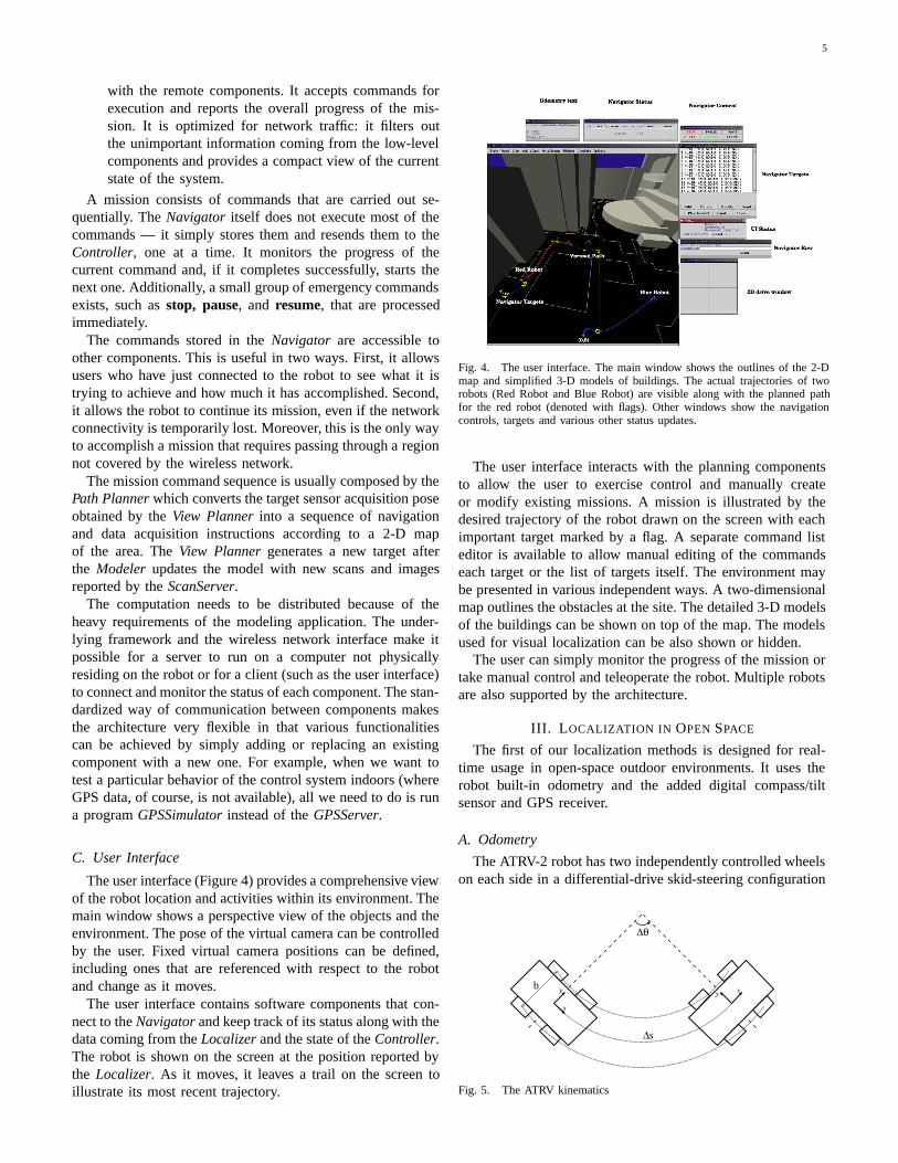
The user interface (Figure 4) provides a comprehensive viewof the robot location and activities within its environment. Themain window shows a perspective view of the objects and theenvironment. The pose of the virtual camera can be controlledby the user. Fixed virtual camera positions can be defined,including ones that are referenced with respect to the robotand change as it moves.

The user interface contains software components that con-nect to the Navigator and keep track of its status along with thedata coming from the Localizer and the state of the Controller.The robot is shown on the screen at the position reported bythe Localizer. As it moves, it leaves a trail on the screen toillustrate its most recent trajectory.

Fig. 4. The user interface. The main window shows the outlines of the 2-Dmap and simplified 3-D models of buildings. The actual trajectories of tworobots (Red Robot and Blue Robot) are visible along with the planned pathfor the red robot (denoted with flags). Other windows show the navigationcontrols, targets and various other status updates.

The user interface interacts with the planning componentsto allow the user to exercise control and manually createor modify existing missions. A mission is illustrated by thedesired trajectory of the robot drawn on the screen with eachimportant target marked by a flag. A separate command listeditor is available to allow manual editing of the commandseach target or the list of targets itself. The environment maybe presented in various independent ways. A two-dimensionalmap outlines the obstacles at the site. The detailed 3-D modelsof the buildings can be shown on top of the map. The modelsused for visual localization can be also shown or hidden.

The user can simply monitor the progress of the mission ortake manual control and teleoperate the robot. Multiple robotsare also supported by the architecture.

III. LOCALIZATION IN OPEN SPACE

The first of our localization methods is designed for real-time usage in open-space outdoor environments. It uses therobot built-in odometry and the added digital compass/tiltsensor and GPS receiver.

A. Odometry

The ATRV-2 robot has two independently controlled wheelson each side in a differential-drive skid-steering configuration

x

y xy

∆θ

∆

b

s

Fig. 5. The ATRV kinematics

6

(Figure 5). The robot moves forward/backward by driving allfour wheels in the appropriate direction. It turns by drivingthe wheels on one side forward and the wheels on theother side backward. Counts from encoders in the motorsare continuously sampled by the firmware and used togetherwith the kinematic parameters (wheel baseline � and the wheelradius �) to compute the robot angular displacement � andtravel distance �� during each sampling interval ����� ���.Then the robot pose is computed according to:

� � � ��

���

� (1)

�� � ��

�����

�� ���� ��

���

�(2)

where, �� � ��� ���� and �, ���� are the robot position and

orientation at time �� and ������ is the 2 x 2 rotation matrixby an angle �.

The above equations reveal the well-known problem in-herent to odometry — minute errors accumulate over timebeyond any reasonable bound. Typically, a robot can accu-rately traverse a few meters but for longer distances relying onodometry becomes impractical. The error can not be boundedwithout the use of an exteroceptive sensor such as our GPSunit discussed in section III-D.

It is possible, nonetheless, to address this problem bylooking at the sources of the errors. Borenstein and Feng haveclassified the errors in two categories: systematic and non-systematic [4]. Systematic errors are defined as ones that aredirectly caused by the kinematic imperfections of the vehicle,while the rest of them are classified as non-systematic. Bothsystematic and non-systematic errors can be addressed.

1) Systematic Errors: According to Borenstein and Feng,two major sources of systematic errors in a differential-driverobot are unequal wheel radii and a misestimated wheelbaseline. Both can be estimated and compensated for byaccurate calibration. We have used their method called theUMBmark to do so [4]. Generally, the point of the performingsuch a calibration is to make sure the the systematic systematicerrors will be reduced to negligible compared to the non-systematic ones.

2) Non-systematic Errors: Examples for causes of non-systematic errors include slippery spots, uneven terrain, sur-face irregularities and over-acceleration. Non-systematic errorscan not be compensated for since they are by definitionrandom and unpredictable. However, we can try to model their“average” behavior so that we keep track of the uncertainty inthe robot pose estimates. We have modeled the robot deviationfrom its expected motion over a sampling period with aGaussian probability distribution with standard deviation pro-portional to the distance traveled. While technically not exact,this is a good enough approximation over a short distanceuntil the robot obtains external observations of its location.This model also has the benefit that it is simple and easy tofuse with the estimates of other sensors in the Kalman filterframework discussed below.

Odometry

Compass

GPS

KalmanFiltertrue orientation

+ compass errors

true pose-- odometry errors

true position+ GPS errors

zk

zk +

+

--h(x)~

z -- h(x)k~

odometry errors+ compass/GPS errors

corrected odometry pose

odometry error estimates

Fig. 6. A diagram of the extended Kalman filter configuration.

B. Digital Compass

The combination of an orientation sensor and odometryhelps estimate the robot motion in 3-D by approximating itwith a piece-wise planar trajectory. Denote by � � �� �� ���

the coordinates of the robot, � � �� � ��� the vector of thethree Euler angles and let ���� be the roll-pitch-yaw matrix

���� � ������������ ��������� (3)

where ������� is the 3 x 3 rotation matrix about axis � by anangle �. Suppose that at time ��, the robot is at position �� andthe compass module provides the orientation measurements��. During the interval ��� �����, no new measurements areavailable and, therefore, the robot pose at time � � ��� �����can be approximated by:

���� � �� ���������� (4)

������ � �������������� ����� (5)

where �� is the angular robot velocity during this time intervaland ����� is computed from (2) as a planar motion relative tothe robot pose at time ��.

C. Kalman Filter

There is some redundancy in the measurements of odometryand the compass module. In addition to the full three degreesof orientation freedom from the compass module, we also getone degree of orientation freedom from odometry. Additionalredundancy is provided by the position fixes from the GPS.To improve on the fusion of the data from the sensors and tokeep track of the uncertainty in these measurements, we haveemployed an extended Kalman filter (EKF) framework [30].As can be seen from Figure 6, we have chosen an indirectformulation, estimating the error in the robot pose (error space)as opposed to the actual pose (total space). This is becausebeing a linear filter, the EKF is better suited to estimateprocesses of low dynamics and the error state in our caseexhibits such a behavior due to the slow drift of the dead-reckoning sensors.

The state vector of the process of the robot motion consistsof the robot pose � � �� ��� which is a 6-vector of the threecoordinates �� �� � and the Euler angles �� � �. The controlinput to the robot is � �� ��� , where � is the translationalvelocity and � is the angular velocity. The process differentialequations are:

�� �

����� ����� ��

��

�� ���� �� ������ �� �

�(6)

7

The matrix ��� is the one that transforms the 3-D angularrate to the Euler angle time derivatives. The vectors �� and� are added zero-mean Gaussian white noise due to effectssuch as discretization and system misrepresentation. We havelinearized about the estimated trajectory from odometry toobtain the Kalman filter prediction equations. This is a goodchoice, since odometry is sampled very frequently and usuallydrifts slowly with the distance traveled. Details about thederivation can be found in [31].

The integration of the compass module in the filter is simple.Its observation model is already linear because the compassdirectly measures three of the six state variables. The moduleis calibrated using publicly available magnetic deviation chartsfor the local area. It is setup to trigger an alarm whenever themagnetic field strength is too low or too high. In such a case,the heading information is unreliable and is ignored.

D. Global Positioning Systems

The EKF framework allows us to easily integrate additionalsensors. The GPS receiver, for example, is added to keepthe position uncertainty from accumulating beyond acceptablelimits. Our GPS unit provides both absolute position informa-tion and the variance of the pose computation. Every time anew fix becomes available, it is incorporated in the EKF byaugmenting the measurement vector with the expected positionof the GPS antenna. Denote the coordinates of the antennawith respect to the robot by �� . The measurement predictionof the absolute position � of the antenna is:

���� � � ������ � (7)

This is linearized to obtain the GPS measurement matrix. Thevariance is also incorporated into the filter in a straight-forwardmanner. The details can be found in [31].

Since the GPS is the only sensor in this method that makesabsolute position measurements, the overall accuracy of themethod depends strongly on the accuracy of the GPS fixes. IfGPS quality deteriorates, the uncertainty in the pose estimatesmay become too large. In such cases, positioning data isneeded from other exteroceptive sensors. But in order to seeksuch data, there has to be a way to detect such situations.This is done by monitoring the variance-covariance matrixrepresenting the uncertainty in the Kalman filter. Each of theeigenvalues of this matrix is the variance of the correspondingelement (position or orientation coordinate) of the state vector.Whenever a new GPS update is processed by the filter, a test isperformed to check if the variance associated with the robotposition is greater than a threshold. If so, we consider thisas an indication that additional data is needed and attempt touse the visual localization method described next. Only theuncertainly in position is considered because if the orientationis wrong it will quickly cause the position error to increasealso.

IV. VISUAL LOCALIZATION

To expand the working range of our localization system,it is sufficient to provide occasional “on-demand” updates

Fig. 7. A sample model (right) of a facade of a building (left).

only when the open-space configuration fails. Visual pose-estimation algorithms are well poised to do that. By actingless frequently and on demand, they can be allowed more timefor image processing operations which can be used to increasethe robustness of the overall system.

This is the underlying idea in the use of our visual local-ization system. As the robot moves, it uses the open-spacelocalization method described in the previous section to keeptrack of its pose along with the uncertainty. As long as it isconfident in these pose estimates, no attempts are made touse vision. If the confidence becomes low, then the robot isallowed to stop and compute a more accurate estimate usingthe vision-based pose estimation method described in thissection. Since this happens relatively infrequently and becauseof the large-scale environments, the time the robot spends inplace doing image processing is small compared to the overalltravel time for a given mission.

A. Environmental Model

The visual pose estimation is based on matching an image ofa building taken by the camera with a model. The environmen-tal model we use a database of smaller-scale facade models.Each facade model depicts the features of a near-planar regionaround a building facade (Figure 7). The features modeled aredominant straight lines — typical and abundant in a human-made environments. All lines are finite segments representedby the 3-D coordinates of their endpoints in a local coordinatesystem, which is registered with the “world” coordinate systemfor the entire site.

In order to be useful, each facade model needs to captureenough features to provide sufficient information for the robotto find its pose. The number of features varies across buildingsbut beyond a certain limit, adding more detail quickly reachesthe point where it does not help the pose estimation. Thereis no need to model every facade or every building either —what is needed is that enough building facades are modeled toallow continuous localization throughout the area of interest.Hence the model we use is simple and compact. For this paper,we have created the models by hand, however, our approachto how to create them automatically is discussed in section VI.

B. Choosing a Model to Use

When visual pose estimation is attempted, a rough estimateof the robot pose is available from the other sensors. Thisestimate is used to search the model data base for the mostappropriate building facade to use for visual localization. Thisis done in two steps according to two criteria: distance andviewing angle (Figure 8).

8

Fig. 8. Choosing a model: A top-down view of modeled facades of buildingsare shown on the map. The two circles show the minimum and maximumdistance allowed. The dotted lines are models that are outside of this range.The dashed lines are models that are within the range but are viewed at avery low (or negative) angle. The solid lines are good to use. The thick oneis chosen because it is closest to the robot.

The first step is to scan through the model database index todetermine the facade models that are within a good distancefrom the robot. Both minimal and maximal limits are imposed:If a building is too close, it may not have enough visiblefeatures on the image; if it is too far, the accuracy of theresult may be low because of the fixed camera resolution.

The second step is to eliminate facade models from thefirst step based on the viewing angle (ranging from ��Æ foran anterior view to ���Æ for a posterior view). Only modelsthat are viewable under a large enough angle are considered.This eliminates both the facades that are not visible (negativeangles) and the ones that are visible at too low an angle toproduce a stable match with the image.

The models that successfully pass this two-step selectionprocess form the set of good candidate models to use. Anysubset of this set can be used in the pose estimation step. Asthe processing time is not trivial, however, we choose to useonly the one that is closest to the robot. Because of the finiteresolution of the camera, this choice is likely to provide themost accurate result.

Finally, the pan-tilt head holding the camera is turnedtoward the chosen facade and an image is taken. The pan andtilt angles are computed from the known rough pose of therobot so that the camera faces the center of mass of the model.In practice, the final orientation of the camera is differentfrom the ideal one because of the uncertainty in the currentpose. However, for the small distances involved and the typicalaccuracy of the pose estimates, the resulting orientation errorof the camera is usually within the tolerance of the processingsteps that follow. Further, since the camera is aimed at thecenter of the model, any small deviation will have minimaleffect.

C. Pose Estimation

At this stage, a pair of an image and a model of the buildingfacade are available and the task is to determine the pose of therobot. Since the camera is tracked by the pan-tilt unit rigidly

N

sj

ej,1ej,2

Pj,1

Pj,2

cameracenter

world coordinatesystem

2D edge onthe image

3D line feature

R, T

distances from3D line endpointsto plane formed

by edge line

li

i

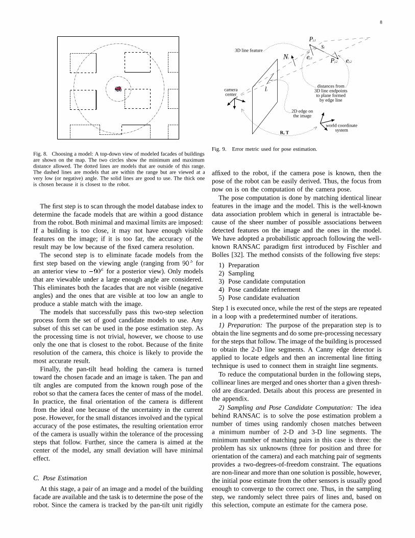
Fig. 9. Error metric used for pose estimation.

affixed to the robot, if the camera pose is known, then thepose of the robot can be easily derived. Thus, the focus fromnow on is on the computation of the camera pose.

The pose computation is done by matching identical linearfeatures in the image and the model. This is the well-knowndata association problem which in general is intractable be-cause of the sheer number of possible associations betweendetected features on the image and the ones in the model.We have adopted a probabilistic approach following the well-known RANSAC paradigm first introduced by Fischler andBolles [32]. The method consists of the following five steps:

1) Preparation2) Sampling3) Pose candidate computation4) Pose candidate refinement5) Pose candidate evaluation

Step 1 is executed once, while the rest of the steps are repeatedin a loop with a predetermined number of iterations.

1) Preparation: The purpose of the preparation step is toobtain the line segments and do some pre-processing necessaryfor the steps that follow. The image of the building is processedto obtain the 2-D line segments. A Canny edge detector isapplied to locate edgels and then an incremental line fittingtechnique is used to connect them in straight line segments.

To reduce the computational burden in the following steps,collinear lines are merged and ones shorter than a given thresh-old are discarded. Details about this process are presented inthe appendix.

2) Sampling and Pose Candidate Computation: The ideabehind RANSAC is to solve the pose estimation problem anumber of times using randomly chosen matches betweena minimum number of 2-D and 3-D line segments. Theminimum number of matching pairs in this case is three: theproblem has six unknowns (three for position and three fororientation of the camera) and each matching pair of segmentsprovides a two-degrees-of-freedom constraint. The equationsare non-linear and more than one solution is possible, however,the initial pose estimate from the other sensors is usually goodenough to converge to the correct one. Thus, in the samplingstep, we randomly select three pairs of lines and, based onthis selection, compute an estimate for the camera pose.

9

The camera pose candidate is found by using the poseestimation method proposed by Kumar and Hanson [33]. Aperspective camera model is used and the calibration param-eters of camera are assumed to be known. An error functionis composed and minimized that quantifies the misalignmentof the 3-D line and its matching 2-D line from the sample.For each 2-D line ��, consider the plane that is formed bythat line and the camera center of projection (Figure 9). Letthe normal to that plane is ��. Suppose, �� is matched withthe 3-D line segment �� whose endpoints ���� and ���� haveworld coordinates ���� and ����. If � and � are the rotationand translation that align the world coordinate system with theone of the camera, then

���� � ��� � �� � ���� � ��� ��� � �� � ���� � ��� (8)

is the sum of squared distances of the endpoints of � � tothe plane formed by �� (Figure 9). The error function thatis minimized is the sum of ���� for the three matching pairs:

���� � � ��

���� ������

���� � (9)

This function is minimized with respect to the six degreesof freedom for the camera pose: three for the rotation � andthree for the translation vector � . The computation followsthe method proposed by Horn [34].

3) Pose Candidate Refinement: The pose candidate refine-ment step uses the consensus set to fine tune the estimate.The consensus set is the set of all matching pairs of 2-Dedge segments from the image and 3-D line segments from themodel that agree with the initially computed pose candidate.

For each 3-D line segment in the model, a neighborhood ofits projection on the image is searched for 2-D edges and theirdistance from the 3-D line segment is computed according to(8). The 2-D edge with the smallest distance is taken to bethe match, if that distance is less than a threshold and if the2-D line is not closer to another 3-D line. If no such 2-D edgeis found, then the 3-D line segment is assumed to have nomatch.

The consensus set is used together with equation (9) tocompute a better pose estimate. This is done iteratively anumber of times (between 1 and 4) starting with a large valuefor the consensus threshold and gradually decreasing it. Thelarge initial value for the threshold makes sure that a roughlycorrect consensus set will be generated initially which will belater refined to eliminate the false positives and increase theaccuracy. The result of the last iteration is the pose candidatethat is evaluated in the next step.

4) Pose Candidate Evaluation: The quality of each posecandidate is judged by a metric ��� � � which quantifies theamount of support for the pose by the matches between themodel and the edge. The idea is to check what portion ofthe model is covered by matching edge lines. The larger thecoverage, the better the pose candidate. Ideally, the entirevisible portion of the model should be covered by matching2-D edge lines.

After the last refinement iteration, the consensus set containspairs of matching 3-D lines from the model and 2-D lines fromthe edges. Consider one 3-D line �� in the consensus set and

its matching 2-D counterpart ��. Let the perspective projectionof �� onto the image be ��� and the orthogonal projection of � �onto ��� be ���. We set contribution ���� of the match between�� and �� to the length of the overlap between � �� and ���. Thus,total portion of the model covered by matching line edges inthe image is:

!��� � � ��

��� ����

���� (10)

The dependence on � and � is implicit as the consensus setand the projections ��� depend on the pose.

Note that the coverage is a quantity which is computed in2-D space. As such, it depends on the scale of the model aswell. If the camera moves away from the building, the visiblesize of the model will diminish and !��� � � will decreaseeven if the match is perfect. Hence normalization needs totake place.

There are two ways to normalize the coverage: divide by thetotal projected length of the model or divide only by the visibleprojected length. The former approach will tend to underratethe correct pose in cases when the model is slightly outside ofthe field of view. The latter approach will do fine in such casesbut will overrate poses for which very little of the model isvisible and the visible portion can easily match arbitrary edgelines. We have chosen to use the latter method and computethe pose evaluation metric as

��� � � � !��� � � � " ��� � � (11)

where " ��� � � is the total length of the visible projection ofthe model on the image.

To avoid the pitfalls of choosing an overrated pose, we usethree criteria by which eliminate a given pose candidate fromconsideration:

1) If the pose candidate is outside of a validation gate, itis immediately rejected as unlikely. The validation gateis determined by the total state estimate of the extendedKalman filter.

2) If the visible portion of the model on the image is lessthan a threshold, the pose is also rejected as there is notsufficient basis to evaluate it, even if it is the correctone. If this is case, the entire localization step is likelyto fail, because the camera was pointed way off-target.

3) If the value ��� � � for the current pose candidate isless than a threshold, the pose is also rejected as thereis insufficient support for it.

Of all the pose candidates that pass the three tests, the onewith the highest score after the loop is the best one and isaccepted to be the correct pose. If no good pose is found, thevisual localization step fails. This is not fatal, however, as therobot simply moves a little further along its route and attemptsanother visual localization step. This is repeated until eitherthe visual localization succeeds, or the GPS picks up a goodsignal and corrects its pose to reduce the uncertainty.

The decision on how many iterations to perform dependson the number of matching lines which is impossible to knowin advance. We terminate the loop after a constant numberof iterations. Our justification for the number of iterations isgiven in the appendix.

10

-20

-15

-10

-5

0

5

10

15

20

25

-30 -20 -10 0 10 20 30 40

BigPlanter

SmallPlanter

Start

End

MapPlanned Trajectory

Actual Trajectory

Fig. 10. The first test run in open space

V. EXPERIMENTS

To demonstrate the functionality of the mobile robot, thesoftware architecture and the software components we wroteas well as to study the performance of the localizationalgorithms, we performed a series of tests with the robotin an actual outdoor environment. The tests took place onthe Columbia University Morningside Campus. Three kindsof tests were performed — one that aimed to evaluate theperformance of the combination of odometry, compass andGPS; another that focused only on the vision component; anda final test that used all sensors.

A. Localization in Open Space

The purpose of these tests were to investigate the accuracyof the open space localization method described in section III.

Arbitrary trajectories were generated by the Path Planneror by the user with the help of the graphical interface, andwere executed. The trajectories were piece-wise linear, withthe robot turning to its next target in place as soon as it reachedthe current one. The maximum translational and rotationalvelocities were 0.5 ��� and 0.4 ����� respectively.

To test the accuracy of the system, two comprehensive testruns were set up to obtain ground truth data. A piece of chalkwas attached at the center of odometry on the bottom of thevehicle so that when the robot moved it plotted its actualtrajectory on the ground. After it completed the task, samplepoints from the actual trajectory were marked at intervals ofapproximately 1 � and measurements of each sample pointwere obtained.

First, a complex desired trajectory of 14 targets and totallength of 210 � was used. (Figure 10 shows the planned andactual trajectories, overlaid on the map of this area of thecampus. The average deviation of the robot from the plannedtrajectory over all sampled points in this run was �����.

The second trajectory consisted of nine targets arrangedin the shape of the digit eight around the two planters inthe center of Figure 10. The trajectory was 132 � long andasked the robot to return to the same place where it started(Figure 11). The average error for this run was ������.

The next experiment also involved the trajectory in Fig-ure 11, but this time of interest was the displacement betweenthe starting and arrival locations. Ideally, the robot had to arriveat its starting location since this was a closed-loop trajectory.

-20

-15

-10

-5

0

5

10

15

20

-5 0 5 10 15 20 25 30 35

BigPlanter

SmallPlanter

Start &End

MapPlanned Trajectory

Actual Trajectory

Fig. 11. The second open-space test run returning to the starting point.

Fig. 12. 3-D models used for localization shown on a 2-D map of the testarea.

Three such runs were performed. The resulting errors were�����, ������, and ������.

It should be noted that the performance of the open-space localization system strongly depends on the accuracyof the GPS data. During the experiment above, the number ofsatellites used were six or seven most of the time, occasionallydropping to five or increasing to eight. The GPS receiver wasworking in RTK float mode in which its accuracy is worsecompared to when it works in RTK fixed mode. The lattermode provides accuracy to within a few centimeters, however,it is typically available when seven or more satellites providegood signal-to-noise ratio over a long period of time.

These results demonstrate that this localization methodis sufficient for navigation in open areas with typical GPSperformance and no additional sensors are needed in suchcases. The location estimate errors in all of the above test runswere within the acceptable range for our urban site-modelingtask.

B. Localization with Vision

To examine the accuracy of the visual localization method,we performed two kinds of tests: one that compares the resultfor each test location with ground truth data, and another,that compares the two results the algorithm produced on twodifferent images taken from the same location.

In both kinds of tests, we wanted to measure the qualityof the location estimation alone and minimize the interferencefrom inaccuracies in the model. Thus, we took care to createaccurate models of the buildings used by scanning theirprominent features with a high-quality electronic theodolitewith nominal accuracy of 2 �� . The features modeled were

11

1 23

4 16

5

6

7

8

9 10

11

12

13

14

15

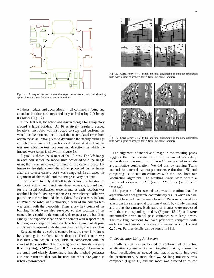
Fig. 13. A map of the area where the experiments were conducted showingapproximate camera locations and orientations.

windows, ledges and decorations — all commonly found andabundant in urban structures and easy to find using 2-D imageoperators (Fig. 12).

In the first test, the robot was driven along a long trajectoryaround a large building. At 16 relatively regularly spacedlocations the robot was instructed to stop and perform thevisual localization routine. It used the accumulated error fromodometry as an initial guess to determine the nearby buildingsand choose a model of one for localization. A sketch of thetest area with the test locations and directions in which theimages were taken is shown in Figure 13.

Figure 14 shows the results of the 16 runs. The left imagein each pair shows the model used projected onto the imageusing the initial inaccurate estimate of the camera pose. Theimage to the right shows the model projected on the imageafter the correct camera pose was computed. In all cases thealignment of the model and the image is very accurate.

Since it is extremely difficult to determine the location ofthe robot with a near centimeter-level accuracy, ground truthfor the visual localization experiments at each location wasobtained in the following manner: An electronic theodolite wasplaced near the robot and the building facade it was lookingat. While the robot was stationary, a scan of the camera lenswas taken with the theodolite. Then, a few key points of thebuilding facade were also surveyed so that location of thecamera lens could be determined with respect to the building.Finally, the expected location of the camera with respect to thebuilding was computed based on the robot estimate of its poseand it was compared with the one obtained by the theodolite.

Because of the size of the camera lens, the error introducedby scanning its surface, rather than the focal center, wasless than 2cm, which is negligible in comparison with theerrors of the algorithm. The resulting errors in translation were������ (min), ����� (max) and ����� (average). These errorsare small and clearly demonstrate that the method generatesaccurate estimates that can be used for robot navigation inurban environments.

Fig. 15. Consistency test 1: Initial and final alignments in the pose estimationtests with a pair of images taken from the same location.

Fig. 16. Consistency test 2: Initial and final alignments in the pose estimationtests with a pair of images taken from the same location.

The alignment of model and image in the resulting posessuggests that the orientation is also estimated accurately.While this can be seen from Figure 14, we wanted to obtaina quantitative confirmation. We did this by running Tsai’smethod for external camera parameters estimation [35] andcomparing its orientation estimates with the ones from ourlocalization algorithm. The resulting errors were within afraction of a degree: �����Æ (min), �����Æ (max) and �����Æ

(average).The purpose of the second test was to confirm that the

algorithm does not generate contradictory results when used ondifferent facades from the same location. We took a pair of im-ages from the same spot at locations 4 and 5 by simply panningand tilting the camera. Both pairs of images were processedwith their corresponding models (Figures 15–16) and wereintentionally given initial pose estimates with large errors.The resulting positions for each pair were compared witheach other and revealed only small discrepancies: ������ and������. Further details can be found in [31].

C. Localization Using All Sensors

Finally, a test was performed to confirm that the entirelocalization system works well together, that is, it uses thevisual localization as needed and that it actually improvesthe performance. A more than ���� long trajectory wascomposed (Figure 17) and the robot was directed to follow

12

1 9

2 10

3 11

4 12

5 13

6 14

7 15

8 16

Fig. 14. Visual localization tests. Each image shows the matching model overlaid as it would be seen from the estimated camera pose. The left image ineach pair shows the rough estimate of the pose that was used to initiate the visual localization. The right image shows the resulting pose of the algorithm.

13

1

2

3

4start finish

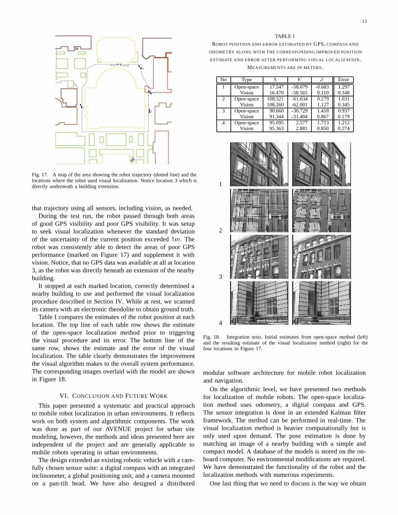
Fig. 17. A map of the area showing the robot trajectory (dotted line) and thelocations where the robot used visual localization. Notice location 3 which isdirectly underneath a building extension.

that trajectory using all sensors, including vision, as needed.During the test run, the robot passed through both areas

of good GPS visibility and poor GPS visibility. It was setupto seek visual localization whenever the standard deviationof the uncertainty of the current position exceeded ��. Therobot was consistently able to detect the areas of poor GPSperformance (marked on Figure 17) and supplement it withvision. Notice, that no GPS data was available at all at location3, as the robot was directly beneath an extension of the nearbybuilding.

It stopped at each marked location, correctly determined anearby building to use and performed the visual localizationprocedure described in Section IV. While at rest, we scannedits camera with an electronic theodolite to obtain ground truth.

Table I compares the estimates of the robot position at eachlocation. The top line of each table row shows the estimateof the open-space localization method prior to triggeringthe visual procedure and its error. The bottom line of thesame row, shows the estimate and the error of the visuallocalization. The table clearly demonstrates the improvementthe visual algorithm makes to the overall system performance.The corresponding images overlaid with the model are shownin Figure 18.

VI. CONCLUSION AND FUTURE WORK

This paper presented a systematic and practical approachto mobile robot localization in urban environments. It reflectswork on both system and algorithmic components. The workwas done as part of our AVENUE project for urban sitemodeling, however, the methods and ideas presented here areindependent of the project and are generally applicable tomobile robots operating in urban environments.

The design extended an existing robotic vehicle with a care-fully chosen sensor suite: a digital compass with an integratedinclinometer, a global positioning unit, and a camera mountedon a pan-tilt head. We have also designed a distributed

TABLE I

ROBOT POSITION AND ERROR ESTIMATED BY GPS, COMPASS AND

ODOMETRY ALONG WITH THE CORRESPONDING IMPROVED POSITION

ESTIMATE AND ERROR AFTER PERFORMING VISUAL LOCALIZATION.

MEASUREMENTS ARE IN METERS.

No Type � � � Error

1 Open-space 17.547 -58.079 -0.683 1.297Vision 16.470 -58.565 0.110 0.348

2 Open-space 108.521 -61.634 0.279 1.031Vision 108.260 -62.001 1.127 0.345

3 Open-space 90.660 -30.729 1.418 0.937Vision 91.344 -31.404 0.867 0.179

4 Open-space 95.095 2.577 1.713 1.212Vision 95.363 2.881 0.850 0.274

1

2

3

4

Fig. 18. Integration tests. Initial estimates from open-space method (left)and the resulting estimate of the visual localization method (right) for thefour locations in Figure 17.

modular software architecture for mobile robot localizationand navigation.

On the algorithmic level, we have presented two methodsfor localization of mobile robots. The open-space localiza-tion method uses odometry, a digital compass and GPS.The sensor integration is done in an extended Kalman filterframework. The method can be performed in real-time. Thevisual localization method is heavier computationally but isonly used upon demand. The pose estimation is done bymatching an image of a nearby building with a simple andcompact model. A database of the models is stored on the on-board computer. No environmental modifications are required.We have demonstrated the functionality of the robot and thelocalization methods with numerous experiments.

One last thing that we need to discuss is the way we obtain

14

the environmental model used for visual localization method.It is tightly coupled to the intended use of the method. Recallthat the work presented here is part of a project whose goalis the creation of a detailed geometric and photometric 3-Dmodel of an urban site. We refer to this detailed model as thedetailed model, as opposed to the localization model used forlocalization.

The detailed 3-D models obtained from the range scans andimages of the buildings are too large and complex since theycapture a lot of detail (Figure 19,center). The modeling processis incremental. At each stage there is a partial model of the siteavailable. During the scan/image registration and process andtheir integration with the existing partial detailed model, a datasimplification step is done which creates a reduced complexitymodel. Its generated for the purpose of the registration ofthe coordinate systems of the range scanner and the camera.This simplified model (Figure 19,right) consists of 3-D linesegments obtained by segmenting the range scans into planarregions and intersecting planes to obtain lines (for details,see [36]). The result of this operation is a set of line segments— the kind that we need for visual localization.

Thus, to create a localization model, only some post-processing is needed of the available 3-D line features. Theset of lines need to be broken into near-planar regions and arepresentative coordinate system needs to be established foreach such region. This is the focus of our current effortsto complete the integration between the modeling and thelocalization aspects of our project.

Note that there is no controversy here about which modelcomes first (the bootstrapping problem). The robot will startfrom a certain location, scan the buildings in view, createtheir partial detailed models and register them with its originalpose. As a result, localization models of some of the scannedfacades will be also available which will allow the robot to gofurther, possibly using the available so far localization models.As it obtains new scans and images and updates the detailedmodel, new localization models will become also availablewhich can be used to localize the robot as it goes farther alongits modeling path.

APPENDIX

NUMBER OF ITERATIONS AND SPEEDUPS IN THE VISUAL

METHOD

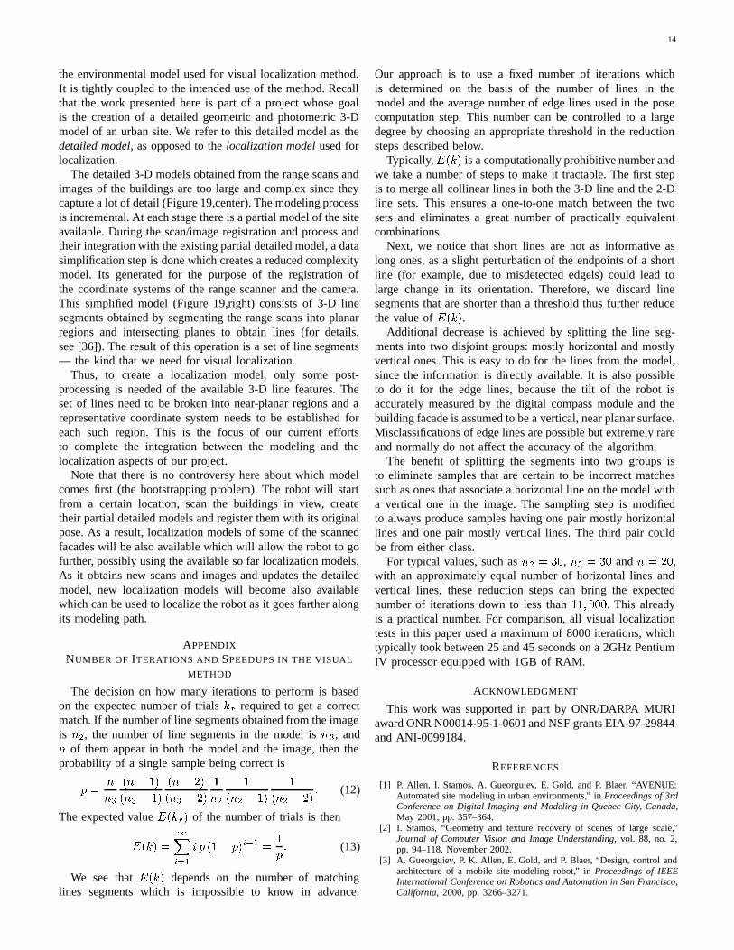
The decision on how many iterations to perform is basedon the expected number of trials �� required to get a correctmatch. If the number of line segments obtained from the imageis #�, the number of line segments in the model is #�, and# of them appear in both the model and the image, then theprobability of a single sample being correct is

$ �#

#�

�#� ��

�#� � ��

�#� ��

�#� � ��

�

#�

�

�#� � ��

�

�#� � ��� (12)

The expected value ����� of the number of trials is then

���� �

�����

% $ ��� $���� ��

$� (13)

We see that ���� depends on the number of matchinglines segments which is impossible to know in advance.

Our approach is to use a fixed number of iterations whichis determined on the basis of the number of lines in themodel and the average number of edge lines used in the posecomputation step. This number can be controlled to a largedegree by choosing an appropriate threshold in the reductionsteps described below.

Typically, ���� is a computationally prohibitive number andwe take a number of steps to make it tractable. The first stepis to merge all collinear lines in both the 3-D line and the 2-Dline sets. This ensures a one-to-one match between the twosets and eliminates a great number of practically equivalentcombinations.

Next, we notice that short lines are not as informative aslong ones, as a slight perturbation of the endpoints of a shortline (for example, due to misdetected edgels) could lead tolarge change in its orientation. Therefore, we discard linesegments that are shorter than a threshold thus further reducethe value of ����.

Additional decrease is achieved by splitting the line seg-ments into two disjoint groups: mostly horizontal and mostlyvertical ones. This is easy to do for the lines from the model,since the information is directly available. It is also possibleto do it for the edge lines, because the tilt of the robot isaccurately measured by the digital compass module and thebuilding facade is assumed to be a vertical, near planar surface.Misclassifications of edge lines are possible but extremely rareand normally do not affect the accuracy of the algorithm.

The benefit of splitting the segments into two groups isto eliminate samples that are certain to be incorrect matchessuch as ones that associate a horizontal line on the model witha vertical one in the image. The sampling step is modifiedto always produce samples having one pair mostly horizontallines and one pair mostly vertical lines. The third pair couldbe from either class.

For typical values, such as #� � ��, #� � �� and # � ��,with an approximately equal number of horizontal lines andvertical lines, these reduction steps can bring the expectednumber of iterations down to less than ��� ���. This alreadyis a practical number. For comparison, all visual localizationtests in this paper used a maximum of 8000 iterations, whichtypically took between 25 and 45 seconds on a 2GHz PentiumIV processor equipped with 1GB of RAM.

ACKNOWLEDGMENT

This work was supported in part by ONR/DARPA MURIaward ONR N00014-95-1-0601 and NSF grants EIA-97-29844and ANI-0099184.

REFERENCES

[1] P. Allen, I. Stamos, A. Gueorguiev, E. Gold, and P. Blaer, “AVENUE:Automated site modeling in urban environments,” in Proceedings of 3rdConference on Digital Imaging and Modeling in Quebec City, Canada,May 2001, pp. 357–364.

[2] I. Stamos, “Geometry and texture recovery of scenes of large scale,”Journal of Computer Vision and Image Understanding, vol. 88, no. 2,pp. 94–118, November 2002.

[3] A. Gueorguiev, P. K. Allen, E. Gold, and P. Blaer, “Design, control andarchitecture of a mobile site-modeling robot,” in Proceedings of IEEEInternational Conference on Robotics and Automation in San Francisco,California, 2000, pp. 3266–3271.

15

Fig. 19. Model acquisition and simplification: an image of a building (left); the 3D model created from the image and a range scan (center); a reducedversion of the same model consisting only of line features (right).

[4] J. Borenstein and L. Feng, “Correction of systematic odometry errorsin mobile robots,” in IROS’95, Pittsburgh, Pennsylvania, August 1995,pp. 569–574.

[5] ——, “Gyrodometry: A new method for combining data from gyrosand odometry in mobile robots,” in Proceedings of IEEE InternationalConference on Robotics and Automation in Minneapolis, Minnesota,1996, pp. 423–428.

[6] S. I. Roumeliotis, G. S. Sukhatme, and G. A. Bakey, “Circumventingdynamic modeling: Evaluation of the error-state Kalman Filter appliedto mobile robot localization,” in Proceedings of IEEE InternationalConference on Robotics and Automation in Detroit, Michigan, 1999,pp. 1656–1663.

[7] S. Cooper and H. F. Durrant-Whyte, “A Kalman filter model for GPSnavigation of land vehicles,” in Proceedings of IEEE InternationalConference on Robotics and Automation in San Diego, California, 1994,pp. 157–163.

[8] J. Schleppe, “Development of a real-time attitude system using aquaternion parametrization and non-dedicated GPS receivers,” Master’sthesis, Department of Geomatics Engineering, University of Calgary,Canada, 1996.

[9] T. Aono, K. Fujii, S. Hatsumoto, and T. Kamiya, “Positioning of vehicleon undulating ground using GPS and dead reckoning,” in Proceedings ofIEEE International Conference on Robotics and Automation in Leuven,Belgium, 1998, pp. 3443–3448.

[10] C.-C. Lin and R. L. Tummala, “Mobile robot navigation using artificiallandmarks,” Journal of Robotics Systems, vol. 14, no. 2, pp. 93–106,1997.

[11] S. Thrun, “Finding landmarks for mobile robot navigation,” in Proceed-ings of IEEE International Conference on Robotics and Automation inLeuven, Belgium, 1998, pp. 958–963.

[12] R. Sim and G. Dudek, “Mobile robot localization from learned land-marks,” in Proceedings of IEEE/RSJ International Conference on Intel-ligent Robots and Systems in Victoria, BC, Canada, October 1998.

[13] A. Kosaka and A. C. Kak, “Fast vision-guided mobile robot navigationusing model-based reasoning and prediction of uncertainties,” Com-puter Vision, Graphics, and Image Processing — Image Understanding,vol. 56, no. 3, pp. 271–329, 1992.

[14] M. Bozorg, E. Nebot, and H. Durrant-Whyte, “A decentralised naviga-tion architecture,” in Proceedings of IEEE International Conference onRobotics and Automation in Leuven, Belgium, 1998, pp. 3413–3418.

[15] J. Neira, J. Tardos, J. Horn, and G. Schmidt, “Fusing range and intensityimages for mobile robot localization,” IEEE Transactions on Roboticsand Automation, vol. 15, no. 1, pp. 76–84, February 1999.

[16] J. Castellanos and J. Tardos, Mobile Robot Localization and Map Build-ing: A Multisensor Fusion Approach. Kluwer Academic Publishers,1999.

[17] S. Thrun, W. Burgard, and D. Fox, “A probabilistic approach toconcurrent mapping and localization for mobile robots,” AutonomousRobots, vol. 5, pp. 253–271, 1998.

[18] F. Dellaert, D. Fox, W. Burgard, and S. Thrun, “Monte Carlo localizationfor mobile robots,” in Proceedings of IEEE International Conference onRobotics and Automation in Detroit, Michigan, 1999, pp. 1322–1328.

[19] H. Durrant-Whyte, G. Dissanayake, and P. Gibbens, “Toward deploy-ment of large scale simultaneous localization and map building (SLAM)

systems,” in Proceedings of International Simposium on Robotics Re-search in Salt Lake City, Utah, 1999, pp. 121–127.

[20] J. Leonard and H. J. S. Feder, “A computationally efficient methodfor large-scale concurrent mapping and localization,” in Proceedings ofInternational Simposium on Robotics Research in Salt Lake City, Utah,1999, pp. 128–135.

[21] J. Borenstein and L. Feng, Navigating Mobile Robots: Systems andTechniques. A. K. Peters, 1996.

[22] H. R. Everett, Sensors for Mobile Robots: Theory and Application.Wellesley, Massachusetts: A. K. Peters, 1995.

[23] D. Kortenkamp, R. P. Bonasso, and R. Murphy, Eds., Artificial Intelli-gence and Mobile Robots: Case Studies of Successful Robot Systems.AAAI Press / The MIT Press, 1998.

[24] G. Dissanayake, P. Newman, S. Clark, H. Durrant-Whyte, andM. Csorba, “A solution to the simultaneous localisation and map building(SLAM) problem,” IEEE Transactions on Robotics and Automation,vol. 17, no. 3, pp. 229–241, June 2001.

[25] J. Guivant, E. Nebot, and H. Durrant-Whyte, “Simultaneous localizationand map bulding using natural features in outdoor environments,”Intelligent Autonomous Systems 6, vol. 1, pp. 581–588, July 2000.

[26] T. Chen and R. Shibasaki, “High precision navigation for 3-D mobileGIS in urban area by integrating GPS, gyro and image sequenceanalysis,” in Proceedings of the International Workshop on Urban3D/Multi-media Mapping, Tokyo, Japan, 1999, pp. 147–156.

[27] R. Nayak, “Reliable and continuous urban navigation using multipleGPS antennas and a low cost IMU,” Master’s thesis, Department ofGeomatics Engineering, University of Calgary, Canada, 2000.

[28] E. Gold, “AvenueUI: A comprehensive visualization/teleoperation appli-cation and development framework for multiple mobile robots,” Master’sthesis, Columbia University, Department of Computer Science, 2001.

[29] Mobility 1.1: Robot Integration Software, User’s Guide, Real WorldInterface, 1999.

[30] R. Brown and P. Hwang, Introduction to random signals and appliedKalman filtering, 3rd ed. John Wiley & Sons, 1997.

[31] A. Georgiev, “Design, implementation and localization of a mobile robotfor urban site modeling,” Ph.D. dissertation, Columbia University, NewYork, NY, 2003.

[32] M. Fischler and R. Bolles, “Random sample consensus: A paradigmfor model fitting with applications to image analysis and automatedcartography,” in DARPA, 1980, pp. 71–88.

[33] R. Kumar and A. R. Hanson, “Robust methods for estimating pose and asensitivity analysis,” Computer Vision Graphics and Image Processing,vol. 60, no. 3, pp. 313–342, November 1994.

[34] B. K. P. Horn, “Relative orientation,” International Journal of ComputerVision, vol. 4, no. 1, pp. 59–78, 1990.

[35] R. Y. Tsai, “A versatile camera calibration technique for high-accuracy 3-D machine vision metrology using off-the-shelf TV cameras and lenses,”Journal of Robotics and Automation, vol. RA-3, no. 4, pp. 323–344,1987.

[36] I. Stamos and P. K. Allen, “Integration of range and image sensingfor photorealistic 3D modeling,” in Proceedings of IEEE InternationalConference on Robotics and Automation in San Francisco, California,2000, pp. II:1435–1440.