localization events-based sample drift correction for ... · localization events-based sample drift...

Localization events-based sample drift correction for localization microscopy with

redundant cross-correlation algorithm Yina Wang,1,2,5 Joerg Schnitzbauer,3,5 Zhe Hu,1,2,5 Xueming Li,4 Yifan Cheng,4 Zhen-Li

Huang 1,2,6 and Bo Huang 3,4,* 1 Britton Chance Center for Biomedical Photonics, Wuhan National Laboratory for Optoelectronics-Huazhong

University of Science and Technology, Wuhan 430074, China 2MoE Key Laboratory for Biomedical Photonics, Department of Biomedical Engineering, Huazhong University of

Science and Technology, Wuhan 430074, China 3 Department of Pharmaceutical Chemistry, University of California, San Francisco, San Francisco, CA 94158, USA

4 Department of Biochemistry and Biophysics, University of California, San Francisco, San Francisco, CA 94158, USA

5These authors contributed equally to this work [email protected]

*[email protected]

Abstract: Highly accurate sample drift correction is essential in super-resolution localization microscopy to guarantee a high spatial resolution, especially when the technique is used to visualize small cell organelle. Here we present a localization events-based drift correction method using a redundant cross-correlation algorithm originally developed to correct beam-induced motion in cryo-electron microscopy. With simulated, synthesized as well as experimental data, we have demonstrated its superior precision compared to previously published localization events-based drift correction methods. The major advantage of this method is the robustness when the number of localization events is low, either because a short correction time step is required or because the imaged structure is small and sparse. This method has allowed us to improve the effective resolution when imaging Golgi apparatus in mammalian cells.

©2014 Optical Society of America

OCIS codes: (180.2520) Fluorescence microscopy; (100.6640) Superresolution; (110.2960) Image analysis.

References and links 1. E. Betzig, G. H. Patterson, R. Sougrat, O. W. Lindwasser, S. Olenych, J. S. Bonifacino, M. W. Davidson, J.

Lippincott-Schwartz, and H. F. Hess, “Imaging intracellular fluorescent proteins at nanometer resolution,” Science 313(5793), 1642–1645 (2006).

2. S. T. Hess, T. P. K. Girirajan, and M. D. Mason, “Ultra-high resolution imaging by fluorescence photoactivation localization microscopy,” Biophys. J. 91(11), 4258–4272 (2006).

3. M. J. Rust, M. Bates, and X. W. Zhuang, “Sub-diffraction-limit imaging by stochastic optical reconstruction microscopy (STORM),” Nat. Methods 3(10), 793–796 (2006).

4. A. Egner, C. Geisler, C. von Middendorff, H. Bock, D. Wenzel, R. Medda, M. Andresen, A. C. Stiel, S. Jakobs, C. Eggeling, A. Schönle, and S. W. Hell, “Fluorescence nanoscopy in whole cells by asynchronous localization of photoswitching emitters,” Biophys. J. 93(9), 3285–3290 (2007).

5. M. D. Lew, S. F. Lee, J. L. Ptacin, M. K. Lee, R. J. Twieg, L. Shapiro, and W. E. Moerner, “Three-dimensional superresolution colocalization of intracellular protein superstructures and the cell surface in live Caulobacter crescentus,” Proc. Natl. Acad. Sci. U.S.A. 108(46), E1102–E1110 (2011).

6. A. Szymborska, A. de Marco, N. Daigle, V. C. Cordes, J. A. G. Briggs, and J. Ellenberg, “Nuclear Pore Scaffold Structure Analyzed by Super-Resolution Microscopy and Particle Averaging,” Science 341(6146), 655–658 (2013).

7. A. R. Carter, G. M. King, T. A. Ulrich, W. Halsey, D. Alchenberger, and T. T. Perkins, “Stabilization of an optical microscope to 0.1 nm in three dimensions,” Appl. Opt. 46(3), 421–427 (2007).

8. R. McGorty, D. Kamiyama, and B. Huang, “Active microscope stabilization in three dimensions using image correlation,” Opt Nanoscopy 2(1), 1–7 (2013).

9. M. Bates, B. Huang, G. T. Dempsey, and X. W. Zhuang, “Multicolor super-resolution imaging with photo-switchable fluorescent probes,” Science 317(5845), 1749–1753 (2007).

#211946 - $15.00 USD Received 12 May 2014; revised 14 Jun 2014; accepted 16 Jun 2014; published 20 Jun 2014(C) 2014 OSA 30 June 2014 | Vol. 22, No. 13 | DOI:10.1364/OE.22.015982 | OPTICS EXPRESS 15982

10. B. Huang, W. Q. Wang, M. Bates, and X. W. Zhuang, “Three-dimensional super-resolution imaging by stochastic optical reconstruction microscopy,” Science 319(5864), 810–813 (2008).

11. S. H. Lee, M. Baday, M. Tjioe, P. D. Simonson, R. B. Zhang, E. Cai, and P. R. Selvin, “Using fixed fiduciary markers for stage drift correction,” Opt. Express 20(11), 12177–12183 (2012).

12. A. Pertsinidis, Y. X. Zhang, and S. Chu, “Subnanometre single-molecule localization, registration and distance measurements,” Nature 466(7306), 647–651 (2010).

13. V. Mennella, B. Keszthelyi, K. L. McDonald, B. Chhun, F. Kan, G. C. Rogers, B. Huang, and D. A. Agard, “Subdiffraction-resolution fluorescence microscopy reveals a domain of the centrosome critical for pericentriolar material organization,” Nat. Cell Biol. 14(11), 1159–1168 (2012).

14. C. Geisler, T. Hotz, A. Schönle, S. W. Hell, A. Munk, and A. Egner, “Drift estimation for single marker switching based imaging schemes,” Opt. Express 20(7), 7274–7289 (2012).

15. M. J. Mlodzianoski, J. M. Schreiner, S. P. Callahan, K. Smolková, A. Dlasková, J. Santorová, P. Ježek, and J. Bewersdorf, “Sample drift correction in 3D fluorescence photoactivation localization microscopy,” Opt. Express 19(16), 15009–15019 (2011).

16. X. M. Li, P. Mooney, S. Zheng, C. R. Booth, M. B. Braunfeld, S. Gubbens, D. A. Agard, and Y. F. Cheng, “Electron counting and beam-induced motion correction enable near-atomic-resolution single-particle cryo-EM,” Nat. Methods 10(6), 584–590 (2013).

17. http://bigwww.epfl.ch/smlm/datasets/index.html. 18. T. W. Quan, P. C. Li, F. Long, S. Q. Zeng, Q. M. Luo, P. N. Hedde, G. U. Nienhaus, and Z. L. Huang, “Ultra-

fast, high-precision image analysis for localization-based super resolution microscopy,” Opt. Express 18(11), 11867–11876 (2010).

19. R. P. J. Nieuwenhuizen, K. A. Lidke, M. Bates, D. L. Puig, D. Grünwald, S. Stallinga, and B. Rieger, “Measuring image resolution in optical nanoscopy,” Nat. Methods 10(6), 557–562 (2013).

20. J. C. Vaughan, S. Jia, and X. W. Zhuang, “Ultrabright photoactivatable fluorophores created by reductive caging,” Nat. Methods 9(12), 1181–1184 (2012).

1. Introduction

Single-molecule switching-based super-resolution fluorescence microscopy (sometimes referred to as localization microscopy) [1–3] has improved the resolution of optical microscopy by more than an order of magnitude and has demonstrated resolution of 20 ~40 nm in the lateral directions [4, 5]. This remarkable gain in the spatial resolution relies on stochastically activating sparse subsets of densely labelled fluorophores and subsequently determining their positions. Typically, thousands or even tens of thousands of raw camera images are necessary to reconstruct the final super-resolution image. Therefore, compared with classical optical microscopy, localization microscopy requires significantly longer data acquisition time. Unsurprisingly, in order to guarantee a high spatial resolution in localization microscopy, the drift between sample and imaging optics (in particular, objective lens) must be corrected (hereafter called sample drift correction), especially for resolving the fine structures of organelles or protein complexes [6].

Current sample drift correction methods differ in how the drift is measured and compensated. Drift compensation can be performed using either active stabilization during acquisition [7, 8] or post-acquisition correction [9, 10], the latter of which has the advantage of not requiring modification to the microscope itself. In both cases, accurate drift measurement is fundamentally important. A common approach for drift measurement is by introducing suitable fiducial markers (normally small fluorescence beads) into the sample. Assuming that the markers are stationary with respect to the target structure, the sample drift can be measured by tracking the marker positions [11, 12]. However, this approach needs additional sample preparation efforts. Moreover, it requires at least one marker to be present in the field-of-view and have no or negligible bleaching during the entire data acquisition, which is particularly difficult to achieve for thick tissue samples.

The alternative approach that does not suffer from these issues is based on cross-correlation analyses of inherent sample structure images, assuming that they do not change during the data acquisition time. This strategy has been implemented with wide-field fluorescence images [9], bright-field images [13], or more directly, the localization events in the reconstructed super-resolution images [10, 14, 15]. In particular, localization events-based cross-correlation method, without any modification to the microscope or the acquisition procedure, has been reported to obtain drift correction accuracy down to sub-5 nm level [15]. However, existing localization events-based cross-correlation methods are extremely vulnerable to the noisy nature of super-resolution images [14]. Consequently, they fail to


provide accurate drift correction when few localization events exist in the field-of-view, for example, when imaging small or sparse organelles (such as the centrosome and the Golgi apparatus) or when short correction time steps are required.

In this paper, we demonstrated a robust method to overcome this problem. This method, named redundant cross-correlation method, is adapted from an algorithm originally used to correct beam-induced motion in cryo-electron microscopy (cryo-EM) [16]. We verified that this method is superior to previously published methods, especially when few localization events can be used for cross-correlation calculation. Furthermore, the redundant method was found to have a robust and stable drift correction performance over a wide range of correction time steps.

2. Methods

2.1 Problem description

We describe the structure of a sample as set of coordinates, s = {xm}, where individual fluorophores are stochastically switched on and localized. Due to the drift (denoted by D) during data acquisition, the observed distribution of fluorophores, S, represents a motion-blurred variant, {xm + Dm} (Fig. 1(a)). In most cases, the only significant drift is translational motion [14, 15], which means that all localization points at the same time point, i, share the same Di regardless of where they are in the view field.

When imaging a fixed sample, the super-resolution images obtained at two time points, Si and Sj, describe the identical structure, despite that each of them contains an incomplete subset of all fluorophore localizations. The localization events-based cross-correlation methods exploit this fact and calculate the cross-correlation function Cij(r) between Si and Sj. When noise is not present, the rij that maximizes the cross-correlation, exactly reflects how much the sample has shifted between these two time points.

( ), where maximizesij ij ij ijC=D r r r (1)

In order to calculate the cross-correlation function using fast Fourier transform, the localization points are usually binned spatially into a 2D histogram of fluorophore density (Figs. 1(a) and (b)). The spatial bin size should be small enough to reveal fine structure features, and should also be large enough so that each bin contains a reasonable number of localization points. The choice of the bin size has been discussed in the literature. For example, for microtubule structures, choosing a bin size between 15 nm and 45 nm is reasonable [14]. The precision of determining r can be better than the bin size, either by fitting the cross-correlation peak with a Gaussian function [10], or by oversampling in the Fourier space [16].

Single molecule localization can be performed only when activated fluorophores in each camera frame are sufficiently sparse. As the result, a single camera frame contains too few localization points for reliable correlation calculation. Therefore, it is essential to combine consecutive camera frames into segments (Fig. 1(b)). The length of the segment, f, thus defines the time step size of drift correction. The required f to achieve a given signal-to-noise ratio (SNR) of cross-correlation map depends on the density of localization points in each frame. When f is too small, the noisy correlation function could contain false maximum that leads outliers in drift estimation (compare Figs. 1(c) and (d)). On the other hand, the drift in each frame within a segment can only be obtained by interpolation. This limitation decreases the precision of drift tracking.


Fig. 1. The effect of correlation time-step size, f, on the cross-correlation map. (a) A super-resolution image of microtubules that contains severe sample drift. The image is spatially binned into a 2D histogram with a bin size of 30 nm. Scale bar: 1 μm. (b) One time segment with f = 1000 frames. (c) The cross-correlation function between the first and the last segments with f = 1000 frames. The white cross shows the auto-correlation peak of the first image. The arrow points out the direction and the amount of the drift between these two intervals. (d) The cross-correlation function between the first and the last segments with f = 100 frames. Note that the SNR in the map is greatly decreased.

2.2 The direct cross-correlation and mean cross-correlation methods

Previously, we have used a simple way to extract the trajectory of sample drift by analyzing the cross-correlation function between each segment and the very first segment, C1j(r) [10], which we refer to as the direct cross-correlation (DCC) method. In this case, each correlation function is fitted with a Gaussian function to determine the position of its maximum, r1j, which is directly used to calculate the sample drift in segment j:

1 .j j=D r (2)

The drift for each frame is obtained by first smoothing the time sequence of Dj by sliding window average and then performing a linear interpolation within each segment.

The mean cross-correlation (MCC) method [14] further considers the correlation between all possible segment combinations Cij(r). A super-resolution data set of N segments will thus produce N × (N – 1) / 2 different cross-correlations. This method also takes into account that measuring the drift from the noisy correlation function will contain a zero-mean error, εij:

.ij ij ij= +r D ε (3)

The sample drift in segments i and j, Di and Dj, can then be related to rij as:

– .ij j i ij= +r D D ε (4)

The optimal solution for Dj should minimize the sum of the square of ε’s. Mathematically, this least square solution is the mean of the measured drift, rij, over i,


( ) / .j i ij N= ΣD r (5)

The stochastic nature of single molecule switching may cause certain pairs of segments to poorly correlate with each other. The resulted noisy correlation functions may contain false maxima which lead to outlier values of rij. These incorrect values of rij are highly detrimental to the accuracy of both DCC and MCC method.

2.3 The redundant cross-correlation method

Recently, a drift correction algorithm that exploits the redundancy among the correlation pairs has been developed for cryo-electron microscopy to fully utilize the high frame rate of the new K2 direct electron detection camera [16]. This algorithm has been used to correct the image shift induced by the electron beam during one exposure, and it has allowed single-particle cryo-EM to reach unprecedented high spatial resolutions. Here, we explore whether this redundancy cross-correlation (RCC) method can be applied to localization-based super-resolution microscopy, noting that the characteristics of cryo-EM images and super-resolution images are very different: cryo-EM images has higher signal but very poor contrast, whereas super-resolution images of individual segments have very low signal level (localization point count) but the underlying structure generally has high contrast.

The RCC method considers a drift model similar to Eq. (4). For consistency, here we express it in a different but equivalent representation as in [16]:

– .ij j i=r D D (6)

The difference, however, is that redundant cross-correlation method treats all N × (N – 1) / 2 equations together as a group of over-determined linear equations in order to solve for the value of N – 1 Di’s (assuming D1 = 0):

=r AD (7)

where r = [r12, r13, …, r23, r24, …, rij]T (1 ≤ i < j ≤ N), D = [D2, D3…, DN]T, and A is the

coefficient matrix set by Eq. (6). rij has been obtained by oversampling Cij(r) through zero-padding at high spatial frequencies in the Fourier space. The least-square solution of D can be calculated by the generalized inverse matrix method

( )–.=

1T TD A A A r (8)

For redundant cross-correlation, outliers in the estimation of rij can be easily excluded without affecting the determination of D due to the over-determined nature of Eq. (7). In practice, after finding the solution of D, the residual error of each rij can be calculated as:

– .Δ =r AD r (9)

Any rij with the residual error larger than a threshold value, Δrmax, will be removed from Eq. (7), unless such removal makes A not fully ranked. Then, Eq. (7) is solved again to obtain a final estimation of D.

Specifically for the implementation in super-resolution microscopy, we further interpolate the drift estimation to individual camera frames with a Spline function. The Δrmax is set to 0.2 times the camera pixel size for all analysis in this paper.

MATLAB code of the three drift correction algorithms can be downloaded at http://huanglab.ucsf.edu/Resources.html.

2.4 Simulation data for image analysis

Simulated localization microscopy data sets were generated from the ground-truth information of an open training data set with microtubule structures [17]. The image consists of a realistic structure of 7 small microtubules (diameter 25 nm) and 1 large microtubule (diameter 40 nm), with a total of 100000 fluorophores distributed in an area of 256 x 256


camera pixels (pixel size: 150 nm). In the simulated localization microscopy data set, an average density of 0.0282 molecules per μm2 per frame were stochastically sampled in each frame. Note the simulated images were considered to be perfect because the simulation data is free of any localization error, background noise and nonspecific labeling.

2.5 Synthesized data for image analysis

A synthesized experimental image data set was used to quantitatively evaluate the performance of the three different drift correction methods. The data set was prepared by the following four steps: (1) An experimental data set was acquired as descried in Section 2.6; (2) The fluorophore localization events were treated with the RCC method to correct for sample drift; (3) the drift-corrected localization events were randomly shuffled between image frames to remove all temporal information and were thus treated as ‘ground-truth’ locations without residual drift; (4) a real drift trajectory, obtained from imaging of fluorescence beads, was added to the ‘ground-truth’ locations to generate the synthesized image data sets.

2.6 Experimental data for image analysis

Golgi experiment data: STORM images of Golgi structures were acquired on home-built super-resolution microscopes. Briefly, the microscopes use an inverted body with oil immersion objectives. Activation lasers at 405 nm and excitation lasers at 642 nm (Vortran Lasers or Coherent) were combined before entering the microscope through a home-built TIRF illuminator. Fluorescence was filtered using a quad-band dichroic mirror (z405/488/561/640rpc, Chroma) and a bandpass filter (ET705/72m, Chroma) before being recorded on a camera. Image focus was stabilized using infrared light reflected at the coverslip/sample interface. The instruments were controlled via home-built software written in Python and Visual Basic. Image analysis was performed with home-built C + + software described previously [10].

More specifically, two Golgi data sets were used in this paper. The data set used in Section 3.3 was acquired on a Nikon Ti-E microscope with an oil immersion objective (Nikon 100x 1.45 Plan Apo λ) and was recorded on an EMCCD camera (iXon + DU897E-CS0-BV EMCCD, Andor). The pixel size at the sample plane is 156 nm. The other data set used in Section 3.4 was acquired on a Nikon Ti-U microscope with an oil immersion objective (Olympus 100x 1.4 Plan Apo). Images were recorded by a sCMOS camera (ORCA Flash 4.0 sCMOS, Hamamatsu). The final pixel size at the sample plane is 121 nm (note there is a pair of relay lenses between the microscopy and camera).

Human retina pigment epithelial (RPE) cells were plated in LabTek-II 8-well chambers, washed twice with warm phosphate buffered saline (PBS), fixed with warm paraformaldehyde (PFA) (4% in PBS, 10 minutes), washed three times with PBS, then permeabilized and blocked (0.5% Triton X-100, 3% bovine serum albumin in PBS, 30 minutes). Next, cells were incubated with primary antibody (Sheep anti human TGN46, AbD Serotec AHP500GT) overnight at 4 degree Celsius. Then the cells were washed three times (10 minutes each, PBS) and incubated with secondary antibody (Donkey anti Sheep, Jackson Immuno Research, 713-005-147, 1.6 µg/ml, labeled with activator Alexa Fluor 405 and reporter Alexa Fluor 647) for 1 hour at room temperature, washed three times (10 minutes each, PBS) and post-fixed (3% PFA and 0.1% gluteraldehyde in PBS, 10 minutes). Finally, the sample was washed three times (PBS) and stored at 4 degree Celsius before imaging.

Microtubules experiment data: the microtubules imaging experiments were performed with a home-built TIRF microscope setup consisting of an Olympus IX-71 inverted microscope (, an oil immersion TIRF objective (Olympus 100x 1.40, UAPON 100XOTIRF, Olympus) and an EMCCD camera (iXon 897, Andor). The sample was fixed BS-C-1 cells and was prepared with similar procedures as the Golgi data sets, where the tubulin were first labeled with mouse anti-β-tubulin antibody (Sigma-Aldrich) and then secondary goat anti-mouse antibody labeled with Alexa 647 (Invitrogen). The dye Alexa 647 was activated by a 405 nm laser diode and excited by a 640 nm diode pumped solid-state laser (both from CNI Laser, China). Data were acquired by the EMCCD camera and the bundled software. The


pixel size at sample plane is 160 nm. The data set was analyzed with a maximum likelihood estimator, the MaLiang method [18].

3.Results and discussions

3.1 Evaluation using simulated data

First of all, we quantified the performance of the three drift correction methods by analyzing simulated error-free localization points of microtubules structures. In the simulation, five localization microscopy movies (each of 1000 frames) were generated as described in Section 2.4 (Fig. 2(a)). Then, a drift trajectory extracted from a real localization microscopy imaging experiment (~5 min acquisition time) was added to these data sets. The maximum amount of the drift is about 150 nm in x direction and about 100 nm in y direction (Fig. 2(b) inset). We used the three cross-correlation methods to extract the drift trajectory from the data sets using a spatial bin size of 15 nm and correlation time steps ranging from 5 to 50 frames. We note that the small end of time steps are applicable only to this ideal simulation conditions but not to real experiments.

We compared the measured drift with the real drift and quantified the precision by the root mean squared (RMS) error between them. Figure 2(b) displays that RCC presents the best precision (minimum RMS = 1.56 nm, compared to 1.63 nm for MCC and 3.39 nm for DCC). Although the performance of RCC and MCC were quite similar with time steps larger than 15 frames, RCC clearly had the edge with very short time steps (5 and 10 frames) for which the number of localization points per segment is small (200 ~400 points). This result indicates that RCC has the best robustness in low SNR scenarios.

In low SNR scenarios, outliers of drift estimation from certain cross-correlation functions become a major issue for RCC and MCC. For example, at 10 frame correction time step, drift estimates by MCC at ~10% of the time points deviated from the true value by more than 5 nm. In contrast, RCC has the capability of exclude false estimations from the calculation. When we skipped the outlier-rejection step in RCC by setting rmax to a very large value, the precision of drift measurement was almost identical to MCC (curve not shown in Fig. 2 because of the full overlap). This result confirmed that the outlier rejection is the main contributor for the superior robustness of RCC compared to MCC.

Fig. 2. The drift estimation precision of the direct, mean and redundant cross-correlation methods in analysing simulated super-resolution images. (a) Simulated perfect super-resolution image. Scale bar: 5 μm. (b) The influence of correlation time step size on drift measurement precision. The inset shows the amount of drift adding to the data sets. Each date point was averaged from five independent measurements. The error bars indicate standard deviations.

3.2 Evaluation using synthesized data

Next, we evaluated the performance using a synthesized experimental data set (see Section 2.5) (Fig. 3(a)). This experimentally acquired data set of Golgi structures in a mammalian cell contains 65067 localization events in 30000 camera frames. The residual drift of this data set


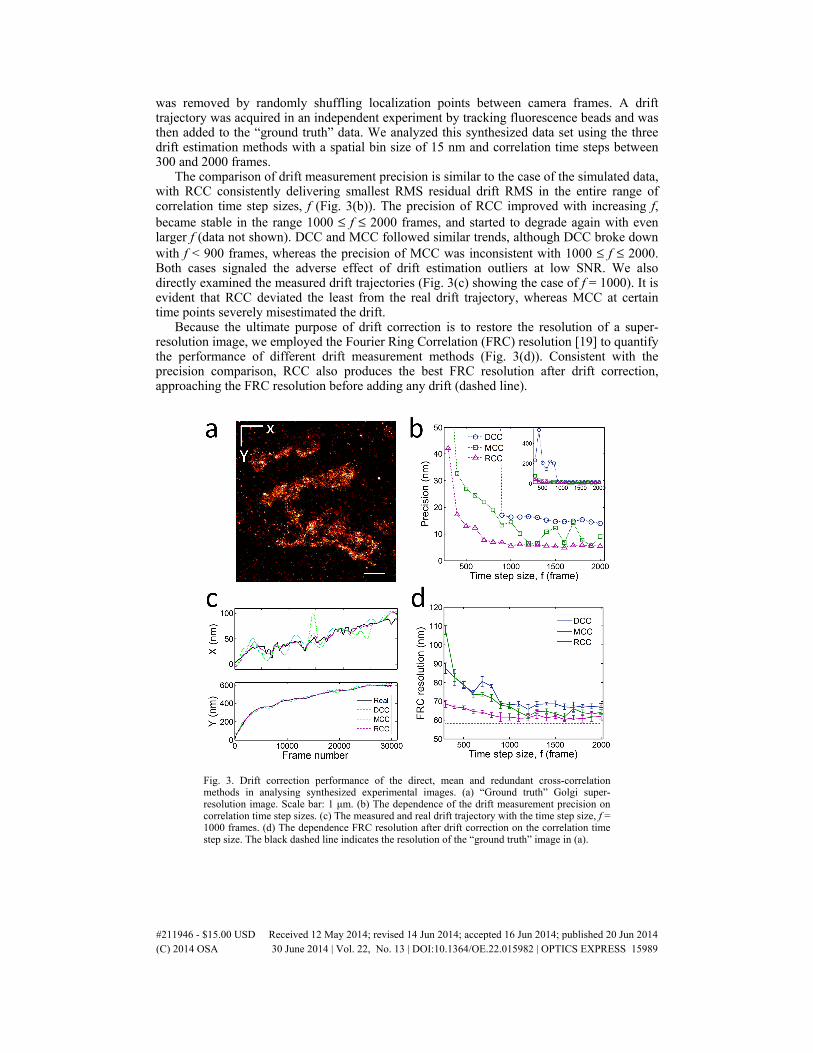
was removed by randomly shuffling localization points between camera frames. A drift trajectory was acquired in an independent experiment by tracking fluorescence beads and was then added to the “ground truth” data. We analyzed this synthesized data set using the three drift estimation methods with a spatial bin size of 15 nm and correlation time steps between 300 and 2000 frames.

The comparison of drift measurement precision is similar to the case of the simulated data, with RCC consistently delivering smallest RMS residual drift RMS in the entire range of correlation time step sizes, f (Fig. 3(b)). The precision of RCC improved with increasing f, became stable in the range 1000 ≤ f ≤ 2000 frames, and started to degrade again with even larger f (data not shown). DCC and MCC followed similar trends, although DCC broke down with f < 900 frames, whereas the precision of MCC was inconsistent with 1000 ≤ f ≤ 2000. Both cases signaled the adverse effect of drift estimation outliers at low SNR. We also directly examined the measured drift trajectories (Fig. 3(c) showing the case of f = 1000). It is evident that RCC deviated the least from the real drift trajectory, whereas MCC at certain time points severely misestimated the drift.

Because the ultimate purpose of drift correction is to restore the resolution of a super-resolution image, we employed the Fourier Ring Correlation (FRC) resolution [19] to quantify the performance of different drift measurement methods (Fig. 3(d)). Consistent with the precision comparison, RCC also produces the best FRC resolution after drift correction, approaching the FRC resolution before adding any drift (dashed line).

Fig. 3. Drift correction performance of the direct, mean and redundant cross-correlation methods in analysing synthesized experimental images. (a) “Ground truth” Golgi super-resolution image. Scale bar: 1 μm. (b) The dependence of the drift measurement precision on correlation time step sizes. (c) The measured and real drift trajectory with the time step size, f = 1000 frames. (d) The dependence FRC resolution after drift correction on the correlation time step size. The black dashed line indicates the resolution of the “ground truth” image in (a).


3.4 Analysis of experimental data

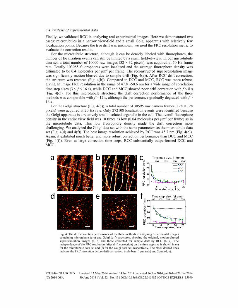
Finally, we validated RCC in analyzing real experimental images. Here we demonstrated two cases: microtubules in a narrow view-field and a small Golgi apparatus with relatively few localization points. Because the true drift was unknown, we used the FRC resolution metric to evaluate the correction results.

For the microtubule structure, although it can be densely labeled with fluorophores, the number of localization events can still be limited by a small field-of-view. In our microtubule data set, a total number of 10000 raw images (32 × 32 pixels), was acquired at 50 Hz frame rate. Totally 103085 fluorophores were localized and the average fluorophore density was estimated to be 0.4 molecules per μm2 per frame. The reconstructed super-resolution image was significantly motion-blurred due to sample drift (Fig. 4(a)). After RCC drift correction, the structure was restored (Fig. 4(b)). Compared to DCC and MCC, RCC was more robust, giving an image FRC resolution in the range of 47.8 ~50.6 nm for a wide range of correlation time step sizes (3 ≤ f ≤ 16 s), while DCC and MCC showed poor drift correction with f < 8 s (Fig. 4(c)). For this microtubule structure, the drift correction performance of the three methods was comparable with f > 12 s, although the performance gradually degraded with f > 16 s.

For the Golgi structure (Fig. 4(d)), a total number of 30595 raw camera frames (128 × 128 pixels) were acquired at 20 Hz rate. Only 272108 localization events were identified because the Golgi apparatus is a relatively small, isolated organelle in the cell. The overall fluorophore density in the entire view field was 10 times as low (0.04 molecules per μm2 per frame) as in the microtubule data. This low fluorophore density made the drift correction more challenging. We analyzed the Golgi data set with the same parameters as the microtubule data set (Fig. 4(d) and 4(f)). The best image resolution achieved by RCC was 45.7 nm (Fig. 4(e)). Again, it exhibited much better and more robust correction performance than DCC and MCC (Fig. 4(f)). Even at large correction time steps, RCC substantially outperformed DCC and MCC.

Fig. 4. The drift correction performance of the three methods in analysing experimental images containing microtubule (a-c) and Golgi (d-f) structures, showing the original, motion-blurred super-resolution images (a, d) and those corrected for sample drift by RCC (b, e). The independence of the FRC resolution (after drift correction) on the time step size is shown in (c) for the microtubule data set and (f) for the Golgi data set, respectively. The black dashed lines indicate the FRC resolution before drift correction. Scale bars: 1 μm (a,b) and 2 μm (d, e).


4. Conclusion

We present a new localization events-based drift correction method for super-resolution microscopy. The method, which we name as redundant cross-correlation method, is based on the combination of a redundant drift model and the calculation the cross-correlation functions of subsets of super-resolution images. Using both simulated and experimental images, we found that this method exhibits much better capability in eliminating drift estimation outliers than the previously reported methods. We further demonstrated that this method is particularly advantageous for super-resolution images of small cell organelles (such as Golgi ribbon structure) and small view-fields, in which the number of localization points in each correction time step is limited. Besides, we inferred that this method will also benefit applications demanding high resolution but require very slow frame rate, for example, when using the ultra-bright fluorophores that have slow switching kinetics [20]. The same algorithm can be easily extended to 3D drift correction using the projection strategy previous described [10, 15]. Specifically, the x and y-drift can be extracted from 2D correlation analysis of the z-projection of the data set. The z-drift can then be extracted from a column-wise 1D z-correlation analysis of the data (after correcting for the xy drift) [10] or from the x and y-projections [15].

Compared to imaging of fixed samples, drift correction for live imaging falls into a different scenario. The potential change of sample shape precludes the use of translational cross-correlation to precisely align images taken at different time points. Nevertheless, correlation analysis at short time scales, during which the structure deformation is small, can still be used to follow sample movement during a long movie.

Acknowledgments

Y. W., Z. H. and Z. L. H. are supported by the National Natural Science Foundation of China (Grant No. 91332103), and the Program for New Century Excellent Talents in University of China (Grant No. NCET-10-0407). J. S. thankfully acknowledges support from a Boehringer Ingelheim Fonds Ph.D. fellowship. B. H. is supported by the NIH Director’s New Innovator Award (1DP2OD008479).


localization events-based sample drift correction for ... · localization events-based sample drift...

Documents