i

Localised Variation of Magnetic Properties of Grain

Oriented Electrical Steels

by

Xin Tong Xu

A thesis submitted to the Cardiff University in candidature for

the degree of Doctor of Philosophy

Wolfson Centre for Magnetics

Cardiff School of Engineering

Cardiff University

July 2014

ii

DECLARATION

This work has not previously been accepted in substance for any degree and is not

concurrently submitted in candidature for any degree.

Signed………………………………………….(candidate) Date ……………………………………..

STATEMENT 1

This thesis is being submitted in partial fulfillment of the requirements for the

degree of PhD.

Signed………………………………………….(candidate) Date ………………………………………

STATEMENT 2

This thesis is the result of my own independent work/investigation, except where

otherwise stated. Other sources are acknowledged by explicit references.

Signed………………………………………….(candidate) Date ………………………………………

STATEMENT 3

I hereby give consent for my thesis, if accepted, to be available for photocopying

and for inter-library loan, and for the title and summary to be made available to

outside organisations.

Signed……………………………………….…(candidate) Date ……………………………………..

iii

Acknowledgements

This work was carried out at the Wolfson Centre for Magnetics, Institute of Energy,

Cardiff School of Engineering, Cardiff University and was funded by Cogent Power,

Tata Steel, UK to which I am grateful for providing the equipments and materials

needed to complete this project.

I would like to express my special thanks to Prof A. J. Moses, for his guidance,

stimulation, encouragement and valuable discussion throughout this investigation.

I am very grateful to Dr J. P. Hall, who supervised this project, for his advice,

comments and alternative views. He has always been a good supervisor and friend

supporting me in many aspects during the time that I studied at Cardiff University.

I wish to thank Mr K. Jenkins, who was my industrial supervisor, for his support and

advice.

I also wish to thank Prof P. Beckley for his helpful suggestions.

I would like to express my greatest thanks to my parents for their love, support and

understanding since I was born.

Last but not least, thanks also go to my colleagues, staff of the electrical workshop,

mechanical workshop and research office, without who this work might has not

been completed by now.

iv

Summary

Localised magnetic flux density, magnetising field and power loss are believed to

distribute non-uniformly in grain oriented electrical steel. Understanding of the

causes of their variation can help reduce the overall power loss of the material.

In this investigation, magnetic domain observation was often used in the study of

domain configuration and crystal orientation of the test specimens. Methods of

domain observation have been studied and compared in order to select the

appropriate method for different parts of the investigation and to improve the

understanding of the image observed.

A less destructive local loss measurement sensor has been built for the

measurement of localised flux density, magnetising field and power loss. The sensor

was tested and evaluated specifically for the measurement of localised magnetic

power loss of the high permeability grain oriented electrical steel.

The results obtained from local loss scanning measurements indicated that localised

flux density and magnetising field can vary substantially in grain oriented electrical

steel under AC magnetisation of 50 Hz. The variation of localised flux density has

been found mainly resulted by grain misorientation and local grain arrangement.

The transverse component of flux density was detected and has been found

increases with increasing grain misorientation. The variation of localised

magnetising field has been found mainly influenced by the localised demagnetising

field due to formation of free magnetic poles at grain boundaries. It has been

proved that both flux density and magnetising field have strong influence on the

distribution of localised power loss.

The study of the effect of domain refinement on distribution of localised flux density

showed that domain refinement by means of ball scribing on one surface of grain

oriented electrical steel can improve the uniformity of distribution of flux density.

However, results also inferred that excessive scribing in a confined area can cause

obvious uneven distribution of flux density in the direction of the specimen’s

thickness.

v

List of Contents

Declarations and Statements ii

Acknowledgements iii

Summary iv

List of contents v

Chapter 1 Introduction 1

Chapter 2 Introduction to Ferromagnetism and Grain Oriented Electrical Steels 4

2.1 Basic terms in magnetism 4

2.2 Ferromagnetic materials and magenetism 6

2.3 Properties and production of grain oriented electrical steels 14

2.4 Power losses in electrical steels 21

Chapter 3 Previous Related Work 25

3.1 Dynamic domain behavior and non-uniform magnetisation 25

3.1.1 Domain wall refinement 25

3.1.2 Grain to grain variation of magnetic permeability 26

3.1.3 Creation and annihilation of 90o surface closure domains 26

3.1.4 Pinning of the 180o domain wall movement 27

3.2 Variation of localised magnetic flux density, magnetic field and

power loss in grain oriented electrical steels

27

Chapter 4 Review of Techniques for Observation of Magnetic Domains in Electrical

Steels

32

32

4.1 Introduction to magnetic domain observation techniques 33

4.2 Bitter pattern 33

4.3 Magnetic force microscope 34

4.4 Magneto-optical Kerr microscopy 35

4.5 Transmission electron microscopy 37

4.6 Scanning electron microscopy 37

4.7 X-ray and Neutron diffraction 38

4.8 Comparison of magnetic domain observation techniques 39

Chapter 5 Review of Local Magnetic Flux Density, Magnetising Field and Power

Loss Measurement Methods

45

5.1 Localised magnetic flux density measurement techniques 45

vi

5.1.1 Search coil method 45

5.1.2 Needle probe method 50

5.2 Local magnetic field measurement techniques 58

5.2.1 Air-cored induction coil sensor 58

5.2.1.1 Previous related works on the H-coil method 59

5.2.2 Hall effect sensor 61

5.2.2.1 Previous related works on the Hall sensor 62

5.3 Local power loss measurement methods 63

5.3.1 Thermometric method 63

5.3.2 B-H loop 65

Chapter 6 Experimental Apparatus 72

6.1 Apparatus for the observation of magnetic domains of electrical

steel samples

72

6.1.1 Static domain imaging using magnetic domain viewer 72

6.1.2 Dynamic domain imaging using Magneto-optical

Kerr microscope

74

6.2 Introduction to the system for measurement of the local magnetic

properties of the single strip electrical steel samples

76

6.2.1 The magnetising system 77

6.2.2 The measurement system 79

6.2.3 The positioning system 82

6.3 Uncertainty analysis 85

Chapter 7 Specimen Selection and Preparation 94

7.1 Selection of test specimens 94

7.2 Preparation of test specimens 96

7.2.1 Preparation of Epstein strips for local loss measurement 96

7.2.2 Preparation of specimens for Kerr microscope observation 96

Chapter 8 Results and Discussion 99

8.1 Introduction 99

8.2 Differences in observed magnetic domain structures found using

domain viewer and magneto-optical Kerr techniques

101

8.3 Domain wall movement at grain boundary in sample of grain

oriented electrical steels

105

8.4 Evaluation of needle probe analysis of flux density in HiB electrical

steel

109

8.4.1 Comparison of flux density measurement using the needle

probe on opposite surfaces of a HiB specimen.

109

vii

8.4.2 Comparison of localised flux density measurement using the

needle probe and search coil methods.

112

8.5 2-D measurement of local magnetic flux density using the

orthogonal needle probe

115

8.6 Influence of induction level on distribution of flux density. 118

8.7 Effect of grain misorientation on variation of localised magnetic flux

density, magnetising field and power loss on grain oriented electrical

steels

122

8.7.1 Localised magnetic flux density, magnetising field and power

loss measurements

122

8.7.2 Correlation between domain wall movement and local

variation of flux density

131

8.8 Effect of domain refinement on distribution of local magnetic flux

density of HiB electrical steel.

134

Chapter 9 Conclusions 145

1

Chapter 1

Introduction

Grain oriented electrical steel is commonly used in power transformers and

high performance rotating electrical machines; it is highly valuable product in

electrical power industries. In the over 100 year’s history of electrical steel, steel

manufacturers have achieved outstanding improvement on magnetic properties of

the steel. However, the power loss occurring in the material during magnetisation

can be as much as 5% of all electrical power generated [1.1]. Therefore, the demand

for better understanding of the causes of power loss grows accordingly.

Grain oriented electrical steel has a polycrystalline structure with a preferred

crystal orientation; such a texture provides low power loss when the steel is

magnetised along its rolling direction. However, it has been reported [1.2-1.8] that

the variation of localised magnetic properties within the polycrystalline structure

can cause increased total power loss.

The study of local magnetic field, magnetic flux density and power loss

variation is essential for understanding the factors that contribute to power loss.

Development of a reliable method for measurement of local magnetic properties is

crucial for the investigation.

2

Considering the demand for greater understanding of effect of localised

variation of magnetic properties on power loss, the main objectives of the

investigation are set as follows:

To study magnetic domain observation techniques and to compare domain

images obtained on the surface of grain oriented electrical steel using these

techniques.

To develop a system for measurement of localised flux density, magnetising

field and power loss of grain oriented electrical steel.

To measure localised flux density, magnetising field and power loss and to

determine factors that lead to their variation.

To investigate the effect of domain refinement on distribution of localised

magnetic flux density.

3

References

[1.1] A. J. Moses, “Characterisation of the Loss behaviour in electrical steels and

other soft magnetic materials”, Proceedings of Workshop on Metallurgy and

Magnetism, Freiberg, Germany, (2004).

[1.2] K. J. Overshott and M. G. Blundell, “Power loss, domain wall motion and flux

density of neighbouring grains in grain-oriented 3% silicon-iron”. IEEE

Transactions on Magnetics, vol. mag-20, pp. 1551 – 1553, (1984).

[1.3] S. Tumanski, “The application of permalloy magnetoresistive sensors for

non-destructive testing of electrical steel sheets”. Journal of Magnetism and

Magnetic Materials, vol. 75, pp. 266 – 272, (1988).

[1.4] A. J. Moghaddam and A. J. Moses, “A non-destructive automated method of

localised power loss measurement in grain oriented 3% silicon iron”, Journal

of Magnetism and Magnetic Materials, vol. 112, pp. 132 – 134, (1992).

[1.5] S. Tumanski and T. Winek, “Measurements of the local values of electrical

steel parameters”, Journal of Magnetism and Magnetic Materials, vol. 174,

pp. 185 – 191, (1997).

[1.6] M. Enokizono, I. Tanabe and T. Kubota, “Localised distribution of two-

dimensional magnetic properties and magnetic domain observation”,

Journal of Magnetism and Magnetic Materials, vol. 196 – 197, pp. 338 – 340,

(1999).

[1.7] K. Senda, M. Kurosawa, M. Ishida, M. Komatsubara and T. Yamaguchi, “Local

magnetic properties in grain-oriented electrical steel measured by the

modified needle probe method”, Journal of Magnetism and Magnetic

Materials, vol. 215 – 216, pp. 136 – 139, (2000).

[1.8] K. Tone, H. Shimoji, S. Urata, M. Enokizono and T. Todaka, “Magnetic

characteristic analysis considering the crystal grain of grain-oriented

electrical steel sheet”, IEEE Transactions on Magnetics, vol. 41, pp. 1704 –

1707, (2005).

4

Chapter 2

Introduction to Ferromagnetism and Grain Oriented

Electrical Steels

2.1 Basic terms in magnetism

A magnetic field H is a region where magnetic material will experience a

force; it can be produced by either electric currents or magnetic poles [2.1]. The

response to the field in the medium is called magnetic induction B, also sometimes

called magnetic flux density [2.2]. It exists in all media whenever there is a magnetic

field. The effective permeability µ of a medium is used to link B and H. Thus, their

relationship is expressed as

HB (2.1)

where B has units of Tesla (T), H has units of Ampere per meter (A/m) and µ is

measured in Henry per meter (H/m). If the media is free space, equation (2.1) can

be written as

HB 0 (2.2)

where 7

0 104 H/m is the permeability of free space. For any other media,

equation (2.1) can be written as

5

HB r0 (2.3)

where r is the relative permeability (dimensionless); it is the ratio of effective

permeability to the permeability of free space 0 , i.e.,

r 0 (2.4)

According to the range of value of r , magnetic materials are mainly

classified into paramagnetic, diamagnetic, anti-ferromagnetic, ferromagnetic and

ferrimagnetic. Ferromagnetic are those with r much higher than unity. Thus, they

have a far wider range of applications than the other classes. In addition, for

paramagnetic and diamagnetic materials r is constant over a substantial range of

applied H. For ferromagnetic material, r varies significantly with the applied H due

to the hysteretic behaviour which is discussed in section 2.2. Typical r values of

some materials are shown in table 2.1.

Classification Material Relative Permeability r

Paramagnetic Air 1.000 000 37

Diamagnetic Copper 0.999 990 00

Anti-ferromagentic Ferrite (manganese zinc) 640

Ferromagnetic Grain oriented electrical steel

(3% Si)

2 000 (H=800 A/m)

Ferrimagnetic Magnetite (e.g. Fe3O4) 4

Table 2.1 Classification of magnetism [2.3].

6

2.2 Ferromagnetic materials and magnetism

Ferromagnetic materials, such as Ni, Fe, Co and some of their alloys, as

mentioned in section 2.1, have very large r . They are formed by regions of aligned

atomic dipoles, even with no external magnetic field presence. The generation of

atomic dipoles in ferromagnetic materials is explained by the band theory.

Electron spin in atoms may have energy level (band), and each energy

level in an atom can contain a maximum of two electrons, and they

must have opposite spin (spin up or spin down). Atoms in

ferromagnetic materials have unfilled 3d energy level, thus leaving

unpaired electrons in this level which gives them magnetic dipoles

[2.1].

Regions of the aligned atomic dipoles are called magnetic domains, and are

illustrated in figure 2.1. The domain theory was first proposed by Weiss in 1906,

and later, Bitter confirmed their existence through observation. He observed

domain patterns on a ferromagnetic material using fine iron powders under an

optical microscope (see chapter 4). As displayed in figure 2.1, atomic dipoles are

aligned parallel in domains where the magnetisation is saturated. The narrow

region where the transformation of dipole alignment takes place is called a domain

wall. The width of the domain wall depends on the equilibrium of exchange and

anisotropy energy. For iron, the width of a 180° domain wall is approximately 160

lattice parameters or 46 nm [2.2].

7

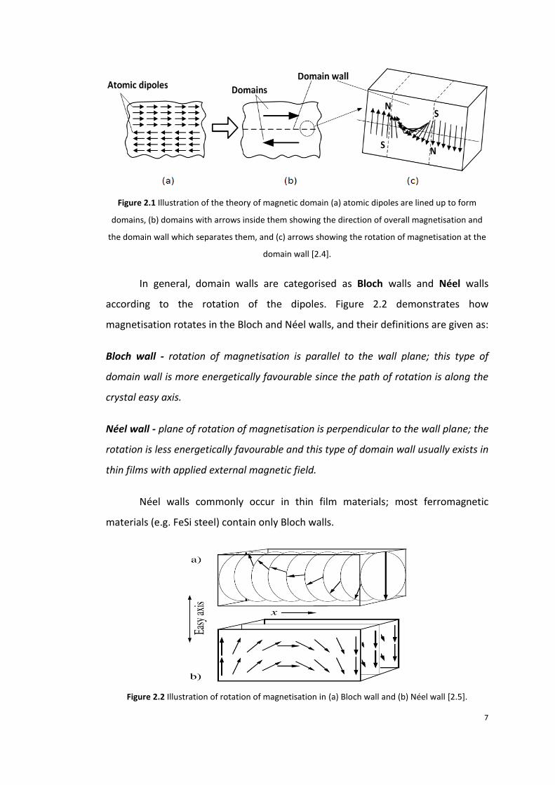
Figure 2.1 Illustration of the theory of magnetic domain (a) atomic dipoles are lined up to form

domains, (b) domains with arrows inside them showing the direction of overall magnetisation and

the domain wall which separates them, and (c) arrows showing the rotation of magnetisation at the

domain wall [2.4].

In general, domain walls are categorised as Bloch walls and Néel walls

according to the rotation of the dipoles. Figure 2.2 demonstrates how

magnetisation rotates in the Bloch and Néel walls, and their definitions are given as:

Bloch wall - rotation of magnetisation is parallel to the wall plane; this type of

domain wall is more energetically favourable since the path of rotation is along the

crystal easy axis.

Néel wall - plane of rotation of magnetisation is perpendicular to the wall plane; the

rotation is less energetically favourable and this type of domain wall usually exists in

thin films with applied external magnetic field.

Néel walls commonly occur in thin film materials; most ferromagnetic

materials (e.g. FeSi steel) contain only Bloch walls.

Figure 2.2 Illustration of rotation of magnetisation in (a) Bloch wall and (b) Néel wall [2.5].

8

Domains exist and arrange themselves to minimise the overall magnetic

energy E, which can be divided into the following energy terms:

𝐸 = 𝐸𝐷 + 𝐸𝝀 + 𝐸𝑒𝑥 + 𝐸𝑘 + 𝐸𝑧 (2.5)

Where,

ED is Magnetostatic energy, which is the energy associated with the leakage

field extending outside the domain.

Eλ is Magnetoelastic anisotropy energy, this is the energy associated with elastic

strains in lattice caused by magnetostriction the magnetic phenomenon

describing the slight change in material dimensions when magnetised.

Eex is Exchange energy, which is the energy related to exchange interaction

between magnetic dipoles; the energy is minimized when all dipoles are

pointing in the same direction.

Ek is Magnetocrystalline anisotropy energy, which is the energy associated with

easy and hard magnetisation direction of a magnetically anisotropy material;

this energy is minimised when material is magnetized along its easy axis. For

iron, this easy and hard axis is described at later context of this section.

Ez is Zeeman energy, which is the energy associated with the externally applied

magnetic field; this energy is minimised when magnetisation of domains are

parallel to the applied field.

Consider a ferromagnetic material containing only a single domain as seen

in figure 2.3 (a). Atomic dipoles are lined up inside the materials and free poles

form on the ends, this creates leakage field and increases magnetostatic energy.

This energy can be reduced if the single domain splits into two domains as

illustrated in figure 2.3 (b). Further reduction is possible by continuing domain

division as illustrated in figure 2.3 (c). However, the process cannot carry on

indefinitely since the exchange energy increases as domain walls are added.

Therefore, energy minimisation accomplished by forming flux-closure domains on

the ends as illustrated in (d) and zero magnetostatic energy is achieved since flux

follows the closed path within the material.

9

Figure 2.3 Illustration of division into magnetic domains.

For iron and silicon iron, walls between the anti-parallel domains are known

as 180° domain walls, and walls between 180° domains and flux-closure domains

are known as 90° walls.

Magnetisation M (A/m) indicates the alignment of magnetic dipoles in a

given direction. When no external field is applied to a ferromagnetic material,

complete saturation magnetisation M0 occurs at 0 K (-273°C). M reduces with

increasing temperature because thermal energy distorts the alignment of diploes.

The alignment of the dipoles disappears completely at the Curie temperature Tc,

and the material becomes paramagnetic. The complete saturation magnetisation

and the Curie temperature of basic ferromagnetic materials are shown in Table 2.2.

Material M0 (106 A/m) Tc (°C)

Iron 1.71 770

Cobalt 1.42 1130

Nickel 0.48 358

Table 2.2 Magnetisation and Curie temperature of ferromagnetic materials.

10

In most ferromagnetic materials, magnetisation M at room temperature is

not much lower than the complete saturation magnetisation M0, so saturation

magnetisation Ms can be measured at room temperature.

In a magnetic material, as illustrated in figure 2.3 (a), the self-produced

magnetic field H due to the formation of free poles is called the demagnetising field

Hd, M and Hd point in opposite directions inside the material. The strength of the

demagnetising field depends on M and the material shape [2.2] and can be

expressed as

MNH dd (2.6)

where dN is the demagnetising factor, which is related to sample geometry (E.g. for

sphere Nd is ～0.3, for a thin plate with field perpendicular to surface Nd is ～0.9

and for a thin plate with field parallel to surface Nd is ～0.1). If an external field Happ

is applied, the self-produced demagnetising field acts against the magnetisation M.

Therefore, the resulting field inside the sample Hin is given by

MNHH dappin (2.7)

Both H and M contribute to the magnetic induction B. In free space, M is

zero, and HB 0 . M in ferromagnetic materials is given by M0 , where the term

M0 is called the magnetic polarisation J (T). The magnetic induction B can be

expressed as

)(000 MHMHB (2.8)

The ratio between M and H is the magnetic susceptibility , which indicates

the level of a material response to an applied field. is expressed as

1 rH

M (2.9)

11

For ferromagnetic materials, values of magnetic permeability and

susceptibility vary according to the magnitude of the applied external field; they

can be obtained from a B-H loop which is shown in figure 2.4.

If an external alternating field H is applied to a ferromagnetic material which

is completely demagnetised so that the domains configure themselves to achieve

the minimum energy stage (position a in figure 2.4), B increases as the domains

respond to the changing field and is represented by equation 2.7. At a lower field,

domains start to reconfigure by creating magnetostatic energy (the energy which

associates with the demagnetising field) which counterbalances the external field.

As a result, domains with dipole alignment near the field grow, and domains with

opposite dipole alignment shrink (position b). At a higher field, dipole alignment

switching occurs in the flux-closure domains (including other less energetically

favourable domains), where dipoles will switch to the direction of the easy axis

which is the preferred crystallographic axis (discussed in detail in figure 2.5 in

section 2.3). Now the material contains only a single domain as dipoles inside it are

all pointing along the easy axis, this is the one closest to the field direction (position

c). At an even higher field where positive saturation magnetisation Ms is reached,

the field energy overcomes the crystal anisotropy energy, leading to the rotation of

dipoles in the domain to align along the field direction (position d).

12

Figure 2.4 Domain process during a cycle of the ferromagnetic material [2.4].

Further increase of the external field will only lead to a slow increase in

magnetic induction due to contribution of air flux ( H0 ) and a further alignment of

imperfectly aligned dipoles caused by thermal activation energy. As a consequence,

r approaches unity. The process a-b-c-d is the initial magnetisation, and the

dashed line is the initial magnetisation curve.

When the field is reduced to zero, magnetic induction drops to the

remanence flux density Br (position e), and the corresponding magnetisation is

called remanence magnetisation Mr. This demonstrates the two characteristics

when a ferromagnetic material is demagnetised, the irreversible initial

magnetisation process and the remaining residual magnetisation after the removal

of the applied external field. They are caused by domain wall pinning at obstacles,

such as dislocations and precipitates [2.6][2.7]. To demagnetise a specimen, an

additional and opposite field must be applied. The field that cancels the residual

magnetisation is the coercive force -Hc. Further increase in the opposed field leads

to negative saturation magnetisation. On reversing the field towards positive

13

saturation, the magnetising path passes the position -Br and Hc on the x and y axis.

This process repeats under the alternating field, and the enclosed loop is called the

B – H loop or the hysteresis loop if the magnetising frequency of the external field is

extremely low.

The area of the B–H loop is proportional to the energy dissipated in the

material per magnetising cycle. Under a.c. magnetisation, the loop becomes

frequency dependent, because additional energy losses can be added to the loop

by rate-dependent eddy current losses and excess losses (discussed in detail in

section 2.4).

Cubic crystalline material, for example iron, has magnetocrystalline

anisotropy. This is sometimes referred to crystal anisotropy, which means that the

material will consume less energy and be easier to magnetise in certain directions

than in others. Therefore, it is important to know the crystallographic axis/axes that

can give the easiest magnetisation. For iron, the easy magnetising axes are <100>

family directions, and figure 2.5 shows the energy required to magnetise iron along

the easy axis and two other important crystallographic axes. A low magnetising field

is needed to reach Ms when magnetising iron along its easy axis.

Figure 2.5 Magnetisation curve for the body centred iron [2.8].

14

As discussed in the domain process in an external field, dipole alignment

switching occurs when the sample is magnetised from position b towards position c

(figure 2.4), because the external field energy overcomes the crystal anisotropy

force. The energy associated with the work done by the field is the crystal

anisotropy energy. This can be calculated from equation 2.9 [2.9], from which the

crystal easy axis can be determined for iron. For cubic crystals, the crystal

anisotropy energy aK is expressed as

...,)()( 22

1

2

3

2

3

2

2

2

2

2

13

2

3

2

2

2

12

2

1

2

3

2

3

2

2

2

2

2

11 aaaaaaKaaaKaaaaaaKEa (2.10)

where 1a , 2a and 3a are the directional cosines of the magnetisation vector with

respect to the three cube edges [100], [010] and [001], 1K , 2K and 3K are the

magnetocrystalline anisotropy constants. Both and K are dimensionless

quantities. For iron, 3K and further terms can be neglected since their values are

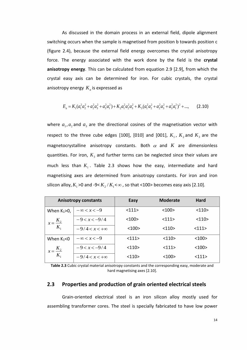
much less than 1K . Table 2.3 shows how the easy, intermediate and hard

magnetising axes are determined from anisotropy constants. For iron and iron

silicon alloy, 1K >0 and -9< 12 / KK < , so that <100> becomes easy axis [2.10].

Anisotropy constants Easy Moderate Hard

When K1>0,

1

2

K

Kx

9 x <111> <100> <110>

<100> <111> <110>

<100> <110> <111>

4/99 x

x4/9

When K1<0

1

2

K

Kx

9 x <111> <110> <100>

<110> <111> <100>

<110> <100> <111>

4/99 x

x4/9

Table 2.3 Cubic crystal material anisotropy constants and the corresponding easy, moderate and hard magnetising axes [2.10].

2.3 Properties and production of grain oriented electrical steels

Grain-oriented electrical steel is an iron silicon alloy mostly used for

assembling transformer cores. The steel is specially fabricated to have low power

15

loss (small B – H area) and high permeability. In addition, small amounts of silicon

are added usually around 3 wt% for lower eddy current loss (see chapter 2.4) by

increasing the electrical resistivity of the material.

Grain oriented steel is made in thin sheets (typical gauge 0.23 – 0.30 mm)

containing grains (typical diameter 5 – 10 mm) which have a similar crystal

orientation as shown in figure 2.6. Goss [2.11] in 1934 found that arranging the

crystals easy axis (110)[001] of grains along the steel rolling direction could increase

its magnetic permeability, thus helping to improve the efficiency of the transformer.

This grain orientation is known as GOSS texture. The (110) plane lies in the sheet

plane, and the [001] direction points approximately parallel to the rolling direction

of the steel; thus, GOSS texture is also called the cube-on-edge structure. The

texture has its highest magnetic permeability and a lower loss when magnetised in

the rolling direction than that of other directions.

Figure 2.6 GOSS steel showing cube-on-edge orientation.

Grain oriented electrical steels are made from hot rolled coils usually

containing 3 wt% Si and a certain amount of grain growth inhibitors. Figure 2.7

shows a schematic diagram of the processing route for making the grain oriented

electrical steels used at Cogent Power Ltd [2.12], which is typical for this class of

material.

16

The initial material is passed through a series of production processes during

the manufacture of electrical steel as shown in figure 2.7, through which the final

product is produced with the desired gauges, grain size and grain orientation.

The main production process is summarised as follows. The initial sheet’s

side is trimmed to remove any rough edges, and it is then annealed, pickled and

oiled ready for cold rolling. The sheet gauge is reduced at the cold rolling mill and

an anti-adhesion layer is coated on the sheet’s surfaces prior anneal at the

decarburising line. During decarburisation, the non-magnetic carbon, which can act

as obstacles pinning domain wall movement and reduce material’s magnetic

permeability, is removed from the steel. Next is the high temperature coil anneal

(HTCA) at around 1200°C, where with the help of restraining primary grain growth

by pre-adopted inhibitors, the steel undergoes a secondary recrystalisation process

for developing the GOSS texture grains. In addition, an electrically insulating coating

known as forsterite is formed on the steel surface during the HTCA. This coating

prevents inter-lamination eddy current from flowing when sheets are stacked in

transformer cores. The steel is cooled after HTCA and goes through to the final

production stage known as the thermal flattening line where a second coating

known as phosphate is applied. The second coating acts primarily to apply

beneficial tensile stress along the rolling direction of the steel. The application of

the tensile stress helps reduce 180o domain wall spacing and lowers energy loss.

17

Figure 2.7 Diagram showing typical process route of making grain oriented electrical steels from the initial hot rolled steel coil [2.12].

18

Grain oriented steel is classified into two types according to the magnetic

permeability; the comparably lower permeability Conventional Grain Oriented

steel (CGO) and the High-permeability Grain Oriented steel (HiB). In general, the

average deviation angle of the easy axis [001] from the rolling direction of the

grains in HiB is less than CGO, approximately 3° for HiB and 7° for CGO. Therefore,

less energy is consumed to magnetise HiB steels than that of CGO along the rolling

direction. Detailed procedures for manufacturing CGO and HiB steels are shown in

table 2.4 and table 2.5 respectively.

The main difference between CGO and HiB steel processing is the grain

growth inhibitors used for obstructing the growth of grains other than GOSS texture.

For CGO steels, manganese sulphide is used as a grain growth inhibitor whereas for

HiB steel, additional aluminium nitride is added to further restrain the growth of

other texture grains.

Grains of HiB steel are much larger that CGO and show wider domain wall

spacing and increased total power loss due to increased eddy current loss [2.13].

Domain refinement, by means of scribing the surface of steel transverse to the

rolling direction, is involved for the production of lower loss HiB steel. A typical

method used in steel manufacture for domain refinement is laser scribing [2.15]. In

this investigation, domain refined specimens were made by the ball scribing

method (see section 8.8), because while the method has the same effect as laser

scribing [2.16], it can be performed more easily in the laboratory environment.

However, scratching damage the material surface and cause additional power loss.

Hence, the optimal loss reduction is obtained by controlling the scribe spacing

which varies depending on the sample condition and scribing parameters, usually

between 4 and 6 mm [2.17][2.18].

19

Conventional Grain Oriented Steel Initial Material: Hot rolled coil approximately 2 mm thick, 3% Si, specified amounts of manganese

and sulphur (grain growth inhibitor: manganese sulphide).

Process Number ( fig. 2.7)

Procedure Purpose of Procedure

1, 2 Anneal at ~950°C, side trim, shot blast, pickle and oil.

To make material suitable for cold rolling and refine metallurgical structure of the hot rolled coil.

3 Cold roll to reduce thickness to ~0.6 mm

To flatten the steel and reduce gauge.

2 Intermediate Anneal at ~950°C To recrystallise and soften the steel for final rolling.

3 Cold roll to final thickness 0.5 – 0.3 mm

To process the steel to finished gauge.

4 Decarburise at ~840°C in wet hydrogen and coat.

To remove remaining carbon from the steel; to further recrystalise and provide silica rich surface layer; to coat with magnesium oxide.

5 High temperature coil anneal at ~1200°C in very dry hydrogen.

To develop GOSS texture by secondary recrystalisation process; to form electrical insulation film; to purify the steel

6 Wash, thermally flatten and phosphate coat.

To remove remaining magnesium oxide; to apply second layer high tensile coating; to product flat and stress free material.

7 Side trim, slit and coil up To get ready for sale.

Table 2.4 Corresponding CGO steel process details shown in fig. 2.7 [2.14].

20

High Permeability Grain Oriented Steel Initial Material: Hot rolled coil approximately 2.3 mm thick, 3.2 – 3.5% Si, specified amounts of

aluminium and other subsidiary elements (grain growth inhibitor: aluminium nitride and manganese sulphide).

Process Number ( fig. 2.7)

Procedure Purpose of Procedure

1, 2

Side trim, pickle, shot blast, anneal at ~1100°C in controlled atmosphere to avoid oxidation, water spray and oil.

To refine metallurgical structure by water quenching after high temperature annealing; to control distribution of aluminium nitride (grain growth inhibitor); to prepare steel for cold rolling.

3 Cold roll to finial thickness To process the steel to finished gauge.

4 Decarburise at ~840°C in wet hydrogen and coat.

To remove remaining carbon from the steel; to further recrystalise and provide silica rich surface layer; to coat with magnesium oxide.

5 High temperature coil anneal at ~1200°C in very dry hydrogen.

To develop GOSS texture by secondary recrystalisation process; to form electrical insulation film; to purify the steel

6 Wash, thermally flatten and phosphate coat.

To remove remaining magnesium oxide; to apply second layer high tensile coating; to product flat and stress free material.

7 Side trim, slit and coil up To get ready for sale.

Table 2.5 Corresponding HiB steel process details shown in fig. 2.7 [2.14]

21

2.4 Power losses in electrical steels

When electrical steels are operating under alternating current (AC)

magnetisation, the total power loss P of the material can be divided into three

components: the hysteresis loss Ph, the classical eddy current loss Pcl and the excess

loss Pe [2.19], so that

eclh PPPP (2.11)

The total power loss in each magnetisation cycle equals the area enclosed

by the B –H loop. When magnetising frequency f→0, the loop contains mostly static

Ph component. Increasing f broadens the loop due to the added dynamic Pcl and Pe

components. Thus, each component plays a vital role in contributing to power loss

at AC magnetisation.

The hysteresis loss is believed to be caused by the pinning of the domain

walls due to the presence of defects (imperfection of the crystal lattice and

impurities) in the material. It can be assumed to be frequency independent (at each

magnetisation cycle) and mainly dependent on the material.

The classical eddy current loss is produced as a result of the changing

magnetic flux density in the laminations of the electrical steel. Assume there is no

skin effect so that flux densities at the surface and within the sheet are the same.

The classical eddy current loss can be calculated using the equation below [2.19]

max

222

4 B

Bf

dBP

pp

cl

(2.12)

where Pcl is classical eddy current loss in units of Joule per cubic meter per cycle

(J/m3 per cycle), pB is the peak flux density, f is the frequency of the

magnetisation in units of Hertz (Hz), d is the material thickness, is the electrical

resistivity of the material and 𝐵𝑚𝑎𝑥 is the saturation magnetisation. The Pcl loss

22

component can be decreased by reducing the material gauge and increasing the

material electrical resistivity.

The excess loss is the difference between the measured loss and the sum of

the static hysteresis loss Ph and the dynamic classical eddy current loss Pcl. The

causes of this excess loss have not been fully understood, but some sources of the

excess loss are widely agreed upon. For example, the micro-eddy current induced

by moving domain walls [2.20], the excess eddy current generated by the unpinning

of the domain walls and the non-uniformity distribution of the local magnetic flux

density.

For electrical steels, when magnetised at peak flux density B , peak

magnetising field H and magnetising waveform frequency f , the total power loss

can be obtained by calculating the B – H loop area. Therefore, the total power loss

tP in units of Watt per kilogram (W/kg) is given by

dtdt

dBH

TP

T

t 0

1

(2.13)

where is the material density and T is the period of magnetisation ( fT /1 ).

23

References

[2.1] B. D. Cullity, “Introduction to magnetic materials”, Addison-Wesley, Reading,

(1972).

[2.2] D. C. Jiles, “Introduction to magnetism and magnetic materials”, Second

edition, Chapman & Hall, London, (1998).

[2.3] Z, Lan, “Physics of Ferromagnetism”, University of Electronic Technology

Press, (1998).

[2.4] S. Somkun, “Magnetostriction and magnetic anisotropy in non-oriented

electrical steels and stator core laminations”, Ph.D. thesis, Cardiff University,

(2010).

[2.5] A. Hubert and R. Schäfer, “Magnetic domains”, Springer, pp. 25 – 26, (1998).

[2.6] R. Comes, M. Gu, M. Khokhlov, J. Lu and S. A. Wolf “Microstructural and

domain effects in epitaxial CoFe2O4 films on MgO with perpendicular

magnetic anisotropy”, Journal of Magnetism and Magnetic Materials, vol.

324, pp. 524-527, (2012).

[2.7] S. Turner, A. Moses, J. Hall and K. Jenkins, “The effect of precipitate size on

magnetic domain behaviour in grain-oriented electrical steels”, Journal of

Applied Physics, vol. 107, p. 09A307, (2010).

[2.8] K. Honda and S. Kaya, “On the magnetization of single crystals of iron”, Sci.

Reports Tohoku Univ., 15, pp.721-753, (1926).

[2.9] S. Chikazumi, “Physics of ferromagnetism”, Oxford University Press Inc.,

New York, (1997).

[2.10] G. Bertotti, “Hysteresis in Magnetism: For physicists, Materials scientists,

and Engineers”, Academic Press, San Diego, (1998).

[2.11] N. P. Goss, “New development in electrical strip steels characterized by fine

grain structure approaching the properties of a single crystal”, Transactions

of the American Society for metals, vol. 23, pp. 511-531, (1935).

[2.12] http://www.orb.gb.com/downloads/cogent_brochure.pdf. Last accessed on

20th June 2013.

[2.13] J. Shilling, “Magnetic properties and domain structure in grain-oriented 3%

Si-Fe”, IEEE Transactions on Magnetics, vol. 10, pp. 195-222, (1974).

24

[2.14] P. Beckley, “Electrical steels”, European Electrical Steels, Newport, (2000).

[2.15] T. Luchi, S. Yamaguchi, T. Ichiyama, M. Nakamura, T. Ishimoto and K. Kuroki,

“Laser processing for reducing core loss of grain oriented silicon steel”,

Journal of Applied Physics, vol. 53, pp. 2410-2412, (1982).

[2.16] P. Beckley and D. Snell, “Low-cost, high-speed domain refinement without

damage to insulative coatings”, Journal of Materials Engineering and

Performance, vol. 3, pp. 209-213, (1994).

[2.17] S. V. Ponnaluri, R. Cherukuri and P. A. Molian, “Core loss reduction in grain-

oriented silicon steels by excimer laser scribing Part I: experimental work”,

Journal of Materials Processing Technology, vol. 112, pp. 199-204, (2001).

[2.18] R. F. Krause, G. C. Rauch, W. H. Kasner and R. A. Miller, “Effect of laser

scribing on the magnetic properties and domain structure of high-

permeability 3% Si-Fe”, Journal of Applied Physics, vol. 55, pp. 2121-2123,

(1984).

[2.19] S. E. Zirka, Y. I. Moroz, P. Marketos and A. J. Moses et al, “Loss separation in

nonoriented electrical steels”, IEEE Transactions on Magnetics, vol. 46, pp.

286-289, (2010).

[2.20] S. Flohrer, R. Schafer, J. McCord, S. Roth, L. Schultz, F. Fiorillo, W. Gunther

and G. Herzer, “Dynamic magnetization process of nanocrystalline tape

wound cores with transverse field-induced anisotropy”, Acta Materialia, vol.

54, pp. 4693 – 4698, (2006).

25

Chapter 3

Previous Related Work

This chapter summarises the previous dynamic domain behaviour, localised

flux density, localised magnetic field and localised power loss studies which are

most relevant to this investigation in the variation of localised magnetic properties

of grain oriented electrical steels.

3.1 Dynamic domain behaviour and non-uniform magnetisation.

Localised variation of magnetic properties can influence the quality of grain

oriented electrical steels, steel with uniform magnetisation is thought to have lower

loss than those with non-uniform magnetisation; thus, it is ideal to have all domain

walls of grain oriented electrical steels move smoothly and at the same speed

under AC magnetisation. In reality, when electrical steel is magnetised at 50 Hz,

domain walls move inhomogeneously at different velocities, resulting non-uniform

magnetisation. This inhomogeneity in domain wall movement is thought to be

mainly due to a number of reasons [3.1-3.3] summarised below:

3.1.1 Domain wall refinement

The number of domain walls increases accordingly with the magnetising

frequency and magnetic induction, which is known as domain refinement and was

first proposed by Polivanow [3.4]. By creating additional domain walls can reduce

the speed of individual domain walls in the process of AC magnetisation and

26

consequently decrease power loss due to the reduction of the eddy current

component. The relationship between domain wall spacing and magnetising

frequency has been studied by Haller [3.5] and Sharp [3.6]; their experimental

results showed that above the frequency of 40 Hz and flux density of 1.2 T, the

relationship between domain wall spacing D and frequency f of sinusoidal

magnetisation can be written as

D ∝1

f (12) 3.1

3.1.2 Grain to grain variation of magnetic permeability.

Grain oriented electrical steels are polycrystalline material containing grains

that are slightly deviated from the rolling direction. The deviation angle varies from

grain to grain. Therefore, when the steel is magnetised under a uniform

magnetising field in the rolling direction of the sheet, domain walls in grains having

smaller deviation angle are more mobile than that of larger deviation angle as

result of the crystal anisotropy.

3.1.3 Creation and annihilation of 90° surface closure domains.

The creation of surface closure domains (or lancet domains) reduces the

magnetostatic energy produced by surface free poles. A small inclination angle

between the easy magnetisation axis of grains and the sheet plane is expected to

develop during coil annealing process (or secondary crystallisation), which leads to

free magnetic poles on either surfaces of the steel. The number of surface closure

domains increases with an increasing inclination angle. These surface closure

domains do not appear at a low magnetisation condition with strong surface

tension and at inclination angles less than 0.5o [3.1]. They appear at high

magnetisation and disappear when magnetisation is low. The process is repeated

under AC magnetisation.

27

3.1.4 Pinning of the 180o domain wall movement.

The 180o main domain walls are pinned by defects when moving in electrical

steel. Such defects could be impurities, surfaces roughness, residual stresses and

precipitates. Since pinning activity increases with an increasing number of closure

domains, it is also expected that the pinning effect is caused by interactions

between 90o closure domains and 180o main domains [3.1].

Ushigami [3.2] observed dynamic domain patterns of a grain oriented

electrical steel using Kerr microscopy. Result of his observations showed that some

180o domain walls were not straight and moving inhomogeneously due to the

pinning effect. Moses [3.7] observed real-time domain wall movement using the

stroboscopic method at different field frequencies. Non-repeatable wall motion

was frequently observed at power frequencies, which indicates that domain wall

pinning occurs irregularly from cycle to cycle magnetisation.

3.2 Variation of localised magnetic flux density, magnetising field

and power loss in grain oriented electrical steels.

Tumanski [3.8-3.9] studied the correlation between power loss and

distribution of localised magnetising field in grain oriented electrical steels. He

found that electrical steel sheets with higher losses also showed broader

distribution of local magnetic field values and higher average field strength values.

Therefore, loss assessment of grain oriented steels can be achieved by analysing

characteristics of the distribution of local magnetic field. In addition, he measured

localised power loss over an area of 10 x 10 mm on a conventional grain oriented

specimen at overall peak flux density of 1.0 T. The result showed that localised

power loss varies as much as 30 %.

Moses [3.10] studied the effects of grain boundaries on the field distribution

of grain oriented steels. He found that the surface fields on two sides of the steel

were similar but not equal since grain boundaries may not at the same position of

the two surfaces. A range of inclination angles of grain boundaries from sheet

28

surfaces was observed and varying from 89° to 26°. As a result, if the sheet is 0.35

mm thick, grain boundaries could be dislocated at the opposite surface by as much

as 1 mm.

Tone [3.11] analysed magnetic characteristic of grain oriented electrical

steel by using computer modelling. The local flux density and magnetic field was

analysed using Finite Element Method (FEM) by taking consideration of the grain

deviation angle, the grain boundary effect and the direction of external field. Local

power losses were calculated from the flux density and magnetic field vectors at an

overall flux density of 1.0 T. The results indicated that the local power loss value is

strongly influenced by the in-plane deviation angle and the relative mismatch angle

between adjacent grains. Higher loss values were found at nearby grain boundary

regions and particularly at high angle grain boundaries, since the magnetostatic

energy is high in those regions.

Overshott [3.12] studied power loss and flux density between neighbouring

grains in grain oriented steel under the overall flux density range from 0.4 to 1.4 T

and external field frequency range from 20 to 120 Hz. The results showed that over

this range of magnetisation, the local flux density can differ by up to 20 % with

respect to overall flux density. Relatively higher flux density and power loss were

measured in well oriented grains in comparison with deviated grains. This is

because flux tends to avoid distribution on the relatively deviated grains by sharing

more flux density between the relatively well oriented grains.

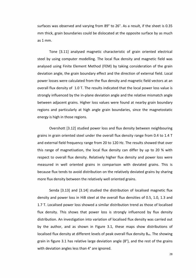
Senda [3.13] and [3.14] studied the distribution of localised magnetic flux

density and power loss in HiB steel at the overall flux densities of 0.5, 1.0, 1.3 and

1.7 T. Localised power loss showed a similar distribution trend as those of localised

flux density. This shows that power loss is strongly influenced by flux density

distribution. An investigation into variation of localised flux density was carried out

by the author, and as shown in Figure 3.1, these maps show distributions of

localised flux density at different levels of peak overall flux density Bm. The showing

grain in figure 3.1 has relative large deviation angle (8°), and the rest of the grains

with deviation angles less than 4° are ignored.

29

At a lower Bm (0.5 T), flux tends to distribute itself along the rolling direction

and avoid the highly mis-oriented grain, resulting elongated flux density patterns as

seen in figure 3.1 (a). At a higher Bm (1.0 and 1.3 T), flux density tends to distribute

more corresponding to the grain structures. Regions of higher flux density appear at

both pole ends of the mis-oriented grain. This is because flux distributed to reduce

the magnetostatic energy generated by magnetic poles at grain boundaries.

Therefore, it was concluded that magnetic poles at grain boundaries affect the non-

uniform distribution of flux density. At an even higher Bm (1.7 T), change in the

domain structures occur, the band domain walls [3.15] start to replace a small

portion of the 180° domains, and magnetostatic energy profile will not be the same

as that of a lower Bm.

Figure 3.1 Contour maps showing distribution of local flux density measured by needle probe at Bm =

0.5, 1.0, 1.3 and 1.7 T [3.14].

30

References

[3.1] T. Nozawa, M. Mizogami, H. Mogi and Y. Matsue, “Magnetic properties and

dynamic domain behaviour in grain-oriented 3 % Si-Fe”, IEEE Transactions

on Magnetics, vol. 32, pp. 572 – 589”, (1996).

[3.2] Y. Ushigami, M. Mizokami, M. Fujikura, T. Kubota, H. Fuji and K. Murakami,

“Recent development of low-loss grain-oriented silicon steel”, Journal of

Magnetism and Magnetic Materials, vol. 254 – 255, pp. 307 – 314, (2003).

[3.3] Z. Xia, Y. Kang and Q. Wang, “Developments in the production of grain-

oriented electrical steel”. Journal of Magnetism and Magnetic Materials, vol.

320, pp. 3229 – 3233, (2008).

[3.4] K. M. Polivanov, “Dynamic characteristics of ferromagnetic materials”, Lzv.

Akad. Nauk SSSR Ser Fiz, vol. 16, pp. 449 – 464, (1952).

[3.5] T. R. Haller and J. J. Kramer, “Observation of dynamic domain size variation

in a silicon-iron alloy”, Journal of Applied Physics, vol. 41, pp. 1034 – 1035,

(1970).

[3.6] M. R. G. Sharp, R. Phillips and K. J. Overshott, “Dependence of loss on

domain-wall spacing in polycrystalline material”, Electrical Engineers,

Proceedings of the institution of, vol. 120, pp. 822 – 824, (1973).

[3.7] A. J. Moses, P. I. Williams and O. A. Hoshtanar, “Real time dynamic domain

observation in bulk materials”, Journal of Magnetism and Magnetic

Materials, vol. 304, pp. 150 – 154, (2006).

[3.8] S. Tumanski, “The application of permalloy magnetoresistive sensors for

non-destructive testing of electrical steel sheets”. Journal of Magnetism and

Magnetic Materials, vol. 75, pp. 266 – 272, (1988).

[3.9] S. Tumanski and T. Winek, “Measurements of the local values of electrical

steel parameters”, Journal of Magnetism and Magnetic Materials, vol. 174,

pp. 185 – 191, (1997)

[3.10] A. J. Moses and S. N. Konadu, “Some effects of grain boundaries on the field

distribution on the surface of grain oriented electrical steels”, International

Journal of Applied Electromagnetic and Mechanics, vol. 13, pp. 339 – 342,

(2002).

31

[3.11] K. Tone, H. Shimoji, S. Urata, M. Enokizono and T. Todaka. “Magnetic

characteristic analysis considering the crystal grain of grain-oriented

electrical steel sheet”, IEEE Transactions on Magnetics, vol. 41, pp. 1704 –

1707, (2005).

[3.12] K. J. Overshott and M. G. Blundell, “Power loss, domain wall motion and flux

density of neighbouring grains in grain-oriented 3% silicon-iron”. IEEE

Transactions on Magnetics, vol. mag-20, pp. 1551 – 1553, (1984).

[3.13] K. Senda, M. Ishida, K. Sato, M. Komatsubara and T. Yamaguchi, “Localized

magnetic properties in grain-oriented electrical steel measured by needle

probe method”, Electrical Engineering in Japan, Vol. 126, No. 4, pp. 942 –

949, (1999).

[3.14] K. Senda, M. Kurasawa, M. Ishida, M. Komatsubara and T. Yamaguchi, “Local

magnetic properties in grain-oriented electrical steel measured by the

modified needle probe method”, Journal of Magnetism and Magnetic

Materials, vol. 215 – 216, pp. 136 – 139, (2000).

[3.15] J. W. Shilling, “Grain boundary demagnetising field in 3% Si-Fe”, Journal of

Applied Physics, vol. 41, pp. 1165 – 1166, (1970).

32

Chapter 4

Review of Techniques for Observation of Magnetic

Domains in Electrical Steels

4.1 Introduction to magnetic domain observation techniques.

Magnetic domain structures can reflect the metallurgical and magnetic

properties of electrical steels. For example, the crystal orientation of grains in grain

oriented electrical steel can be determined from the alignment of the 180° domain

walls and the amount of the lancet domains distributed on the surface of the steel.

Bitter [4.1] made the first attempt to observe domain structures on the

surfaces of iron, nickel and cobalt crystals using a magnetic powder technique.

However, the initial pattern he observed using the technique was not clear and

could not be fully interpreted at the time until Landau and Lifshitz developed their

free energy theory of magnetism and made the correct theoretical predictions of

domain structure in ferromagnetic material (cited in [4.2]).

Williams [4.3] used electrolytic polishing and observed clear domain

patterns on the surface of single crystal silicon iron showing strong agreement with

Landau and Lifshitz’s predictive model. Thereafter, domain observation has been

frequently used for the study of magnetic materials.

33

In general, techniques for observation of magnetic domains of electrical

steels can be classified into three methods based on their observation mechanism.

They are:

(1) Magnetic stray field sensitivity methods

- Bitter pattern

- Magnetic force microscope (MFM)

(2) Magnetic polarisation sensitivity methods

- Magneto-optical Kerr microscope

- Transmission electron microscope (TEM)

- Scanning electron microscope (SEM)

(3) Crystal lattice distortion sensitivity methods

- Neutron diffraction

- X-ray

Each technique has unique advantages and limitations as outlined in the

following sections. The aim of this chapter is to study techniques for observation of

electrical steels and to compare and select the suitable techniques for this

investigation.

4.2 Bitter Patterns

In 1932, Francis Bitter [4.1] demonstrated a technique for the observation of

magnetic structures on iron, nickel and cobalt materials using 1μm diameter Fe2O3

particles suspended in ethyl acetate. The technique was a development based on

the “old magnetic powder method” (cited in [4.1]), but with a much smaller particle

size to reveal details, and the use of low viscosity ethyl acetate as a solution to

improve the particle mobility so that they can settle quickly in the stray field.

Although there was no definite explanation of the observed pattern at that time

due to a lack of understanding of the domain concept, the historical significance of

the technique’s development is very important.

34

The Bitter method senses a stray field formed by the free poles on the

sample surfaces. Thus, the contrast of the image relies on the interaction between

the field and the ferromagnetic particles. Poor image contrast is often obtained

using the Bitter method, thus the demand for improvement of the technique grows

accordingly [4.4] (see modified Bitter technique outlined in chapter 6).

4.3 Magnetic Force Microscope

A magnetic force microscope (MFM) is a high-resolution scanning probe

microscope which is designed for viewing micro and nano sized structures. In 1986,

based on the concept of a scanning tunnelling microscope [4.5], Binnig et al. [4.6]

developed the atomic force microscope (AFM). The microscope allows the surface

topography of a sample to be imaged through a non-conductive method. During the

scanning, an AFM probe, which consists of a force detective tip and force sensitive

cantilever, is used to detect near-surface atomic forces. The cantilever deflects as

the tip moves across the scanning surface, and the angle of deflection is sensed by a

laser beam and a photo-detector so that the topograpic image can be plotted.

Later, based on the success of the AFM, Sáenz [4.7] and Martin [4.8]

individually developed the MFM microscope for the observation of magnetic

patterns. In the MFM, magnetic images are obtained by using an MFM tip which is

typically made from an AFM tip and coated with a thin layer of magnetic material.

During the scanning, the MFM tip interacts with the leakage field above the surface

of the magnetic material to produce an image showing stray field profile of the

scanning area. The highest spatial resolution of the MFM is reported at less than

10nm [4.9]. This enables micro and nano magnetic structures (e.g. domain walls) to

be studied easily. Moses [4.10] made an attempt to observe grain boundary in grain

oriented electrical steel using the MFM. A fine finger print pattern was found which

has not yet been understood, but it has shown that the technique could provide

useful information relating to the micro magnetism of electrical steels.

MFM is a near-surface raster scanning microscope, so a moderate sample

preparation is necessary to obtain a reasonable smooth surface for preventing

35

contact damage and improving signal to noise ratio. The microscope offers typical

scanning area of up to 100 x 100 µm, which is rather small compared to the

magnetic features of grain oriented electrical steels.

4.4 Magneto-optical Kerr Microscopy

The observation principle of magneto-optical Kerr microscopy is based on

the Kerr Effect [4.11], which was discovered by John Kerr in 1877 following the

discovery of the well known Faraday Effect. The Faraday Effect occurs when the

polarisation angle of a plane polarised light, propagating through a medium

containing a magnetic field, changes because of the presence of the field. The Kerr

effect describes the same concept but is a reflection effect rather than transmission,

that is, a change in the polarisation angle of plane polarised light when the light is

reflected from surface of a magnetic material.

To observe domain patterns using a Kerr microscope, the concept of Lorentz

force is applied and an example is shown in figure 4.1. When a beam of plane

polarised light is projected on a sample containing magnetic domains, a secondary

light wave is induced by the Lorentz moment νLor as stated in Huygens’ Principle

(cited in [4.12]). This secondary light is polarised perpendicular to the normal

reflected light rotated by an angle of θk. If the observed sample contains anti-

parallel domains such as on the surface of grain oriented steel, then -θk is obtained

for light reflected from the neighbouring domains, thus, by using an analyser to

block the entry of light with either +θk or - θk, a image contrast showing the

direction of the magnetisation of the observation area is formed. As a result, the

domain pattern on the surface of a sheet of electrical steel can be revealed as in

figure 4.1 using the Kerr microscope.

36

Figure 4.1 Illustration of the longitudinal Kerr Effect.

Since the Kerr microscope is an optical based apparatus, its resolution is

limited by the wavelength of light (~200 nm). Takezawa [4.13] demonstrated that a

higher resolution of 150 nm can be obtained by utilising UV light source in the Kerr

microscope.

The main drawback of this method is that the technique involves time-

consuming metallurgical sample preparation (see section 7.2). Thereafter the

metallurgical preparation, a stress relief anneal is required to remove residual stress

that added during the preparation for restoring domain pattern.

The Kerr microscope is a real time direct magnetisation observation

apparatus. For this reason, Kerr microscopy has been intensively used for the study

of domain wall movements in electrical steels [4.14 - 4.19].

Following the development of high speed cameras such as a charge-coupled

device (CCD) or complementary metal oxide semiconductor (CMOS) cameras,

dynamic domain images at or above power frequencies (≥50Hz) can be captured.

These cameras can provide an improved recording speed and resolution in

comparison to conventional cameras, such as Newicon tube cameras.

Moses [4.16] described an instrument for real time dynamic domain

observation on the surface of electrical steels using the Kerr microscope and a

CMOS camera (with recording speed of up to 1800 frames per second) at

37

magnetisation frequencies of up to 50 Hz. Such real time observation provides

useful information for study of non-uniform wall mobility from grain to grain.

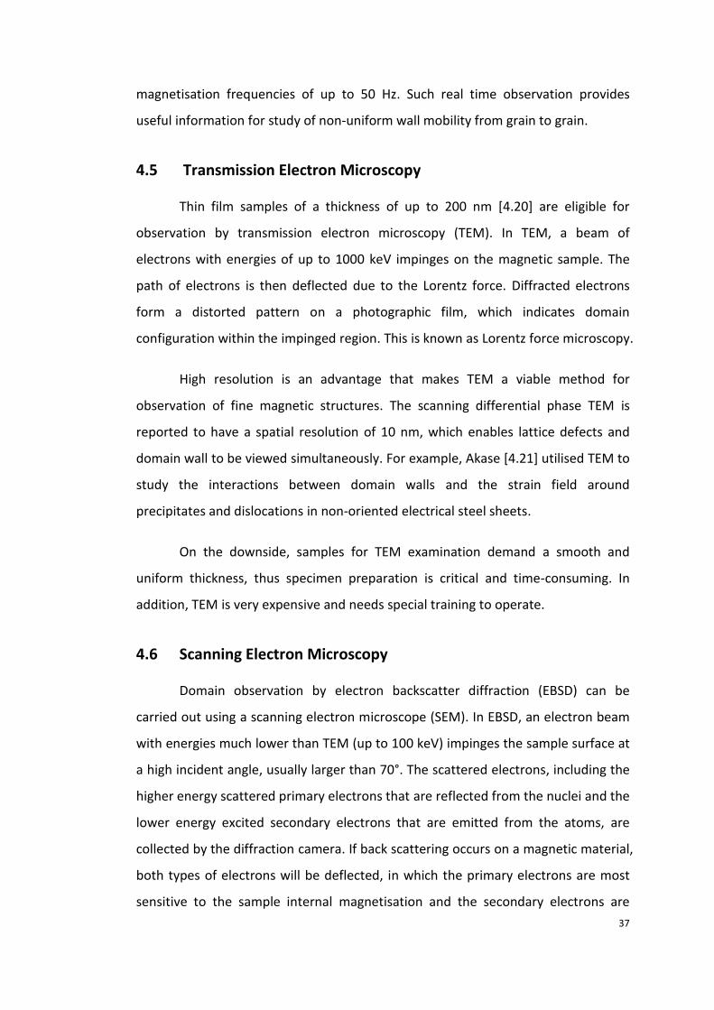
4.5 Transmission Electron Microscopy

Thin film samples of a thickness of up to 200 nm [4.20] are eligible for

observation by transmission electron microscopy (TEM). In TEM, a beam of

electrons with energies of up to 1000 keV impinges on the magnetic sample. The

path of electrons is then deflected due to the Lorentz force. Diffracted electrons

form a distorted pattern on a photographic film, which indicates domain

configuration within the impinged region. This is known as Lorentz force microscopy.

High resolution is an advantage that makes TEM a viable method for

observation of fine magnetic structures. The scanning differential phase TEM is

reported to have a spatial resolution of 10 nm, which enables lattice defects and

domain wall to be viewed simultaneously. For example, Akase [4.21] utilised TEM to

study the interactions between domain walls and the strain field around

precipitates and dislocations in non-oriented electrical steel sheets.

On the downside, samples for TEM examination demand a smooth and

uniform thickness, thus specimen preparation is critical and time-consuming. In

addition, TEM is very expensive and needs special training to operate.

4.6 Scanning Electron Microscopy

Domain observation by electron backscatter diffraction (EBSD) can be

carried out using a scanning electron microscope (SEM). In EBSD, an electron beam

with energies much lower than TEM (up to 100 keV) impinges the sample surface at

a high incident angle, usually larger than 70°. The scattered electrons, including the

higher energy scattered primary electrons that are reflected from the nuclei and the

lower energy excited secondary electrons that are emitted from the atoms, are

collected by the diffraction camera. If back scattering occurs on a magnetic material,

both types of electrons will be deflected, in which the primary electrons are most

sensitive to the sample internal magnetisation and the secondary electrons are

38

most sensitive to the stray field over the sample surface. In addition, in order to

image magnetic domains using backscattered electrons, a direction and energy

sensitive collector is also needed to extract the magnetic information.

The other worth to mention, direct domain observation method that uses

SEM is the scanning electron microscopy with polarisation analysis (SEMPA). It is

known that the secondary electrons emitted from magnetic sample have a spin

polarisation which reflects the net spin density in the material [4.22]. The spin

density, in turn, is directly related to the magnetisation of the material. In a similar

way as the EBSD, by measuring secondary electron spin polarization, magnetic

domains of magnetic samples can be reviewed using SEMPA.

The SEM method has a higher penetration depth and is less sensitive to

surface roughness than that of TEM; thus, it is considered to be more bulk

representative. Endo [4.23] observed domain patterns at about a depth of 10 µm

from surface of grain oriented steel using the EBSD that was carried out at 160 kV.

4.7 X-ray and Neutron diffraction

The radiation sources of X-ray and neutron diffraction can be unique and

distinguished from the TEM and SEM techniques. Synchrotrons (a combination of

electromagnetic radiations that are accelerated by synchrotrons) and thermal

neutrons are used respectively. The imaging method requires radiation to pass

through the specimen, and on the other side, diffraction patterns are formed on the

screen containing information with respect to the structure of crystal lattice. If the

specimen is magnetic, then a distorted lattice structure is observed due to the

presence of magnetostrictive strains. The domain image can be obtained by

scanning the area of interest. There is a distinct difference between X-ray and

neutrons that arises from the spin-orbit interaction of neutrons with magnetic

materials, this results in additional Bragg peaks that allow identification of magnetic

state (antiferromagnetic or ferromagnetic).

39

Both the X-ray and neutron diffraction techniques can reach a higher

penetration depth than that of TEM and SEM due to the application of higher

energy particles. Thus, the magnetic structure within electrical steels can be easily

revealed. Withers studied [4.24] the penetration depth of synchrotron and neutron

diffraction, for an iron based substrate. It was estimated that the penetration depth

of synchrotron is up to 9 mm and neutron is up to 30 mm.

The main drawback of the X-ray and neutron diffraction technique is the

safety concern. High radiation may damage the sample, and a radiation-proof shield

is necessary.

4.8 Comparison of magnetic domain observation techniques

The techniques for observing static and dynamic domain structures on the

surface or within electrical steels are compared in table 4.1. In summary, the stray

field sensitive, low resolution Bitter technique is most suitable for imaging relatively

large domain patterns on the surface of grain oriented steels, both with or without

insulation coatings. The high magnification, high resolution, stray field sensitive

MFM is suitable for revealing the fine domains of non-oriented steels with and

without coatings. For dynamic domain observation on electrical steel, magneto-

optical Kerr microscopy is the most appropriate method due to real time recording

characteristic. TEM and SEM are direct magnetisation sensing techniques for

observing micro and nano magnetic features and therefore the specimen must be

prepared to a high finishing condition. X-rays and neutrons are powerful methods

for the study of the magnetisation of a bulk sample; however care must be taken

due to the high risk of radiation.

In this investigation, the static domain patterns of HiB steel specimens were

observed using the Bitter technique because the method enables grain boundary

and domain pattern to be revealed simultaneously across the entire loss scanning

area on Epstein specimens outlined in chapter 8. Dynamic domain patterns of HiB

steel at 50 Hz magnetisation were studied using the Magneto-optical Kerr

40

microscope. The real time direct magnetisation observation characteristic enables

surface domain wall movement to be imaged at power frequency.

In addition, a detailed study of the Bitter technique and the magneto-optical

Kerr miscroscope for observation of domains in HiB specimen is carried out in

chapter 8 and 9, in which inconsistency in domain patterns obtained using the Bitter

technique and the Magneto-optical Kerr microscope on the same HiB specimen is

discussed. Therefore, improved understanding in observation mechanism of both

techniques is achieved.

41

Table 4.1 Comparison of magnetic domain observation techniques. (adapted from [4.12])

Observation techniques

Level of Sample

preparation

Assessment on direction of

magnetisation

Observation through

coatings of steels

Sensitivity to change in

magnetisation

Spatial resolution

Dynamic observation

Recording time

Used in this study

Bitter very low indirect yes excellent Low (1μm) no Few secs yes

MFM Low -

moderate indirect yes good

High (10 nm)

no Tens of

mins no

Kerr moderate direct no fair Moderate (0.1 μm)

yes Real-time yes

TEM very high direct no good Very high (1

nm) possible Few secs no

SEM high direct no good High

(10 nm) possible Few secs no

X-ray, Neutron

low indirect no poor Very low (5 μm)

no Few mins no

42

References

[4.1] F. Bitter, “Experiments on the nature of ferromagnetism”, Physical Review,

Vol. 41, pp. 507 – 515, (1932).

[4.2] R. Carey and E. D. Isaac, “Magnetic domains and techniques for their

observation, The English University Press Ltd, London, (1966).

[4.3] H. J. Williams, R. M. Bozorth and W. Shockley, “Magnetic domain patterns

on single crystals of silicon iron”, Physical Review, vol. 75, pp.155-171,

(1949).

[4.4] R. J. Taylor, A. De Fisica, Serie B, Vol. 86, p. 126, (1990).

[4.5] P. W. Epperlein, H. Seifert and R. P. Huebener, “Two-dimensional imaging of

the current-density distribution in superconducting tunnel junctions”,

Physics Letters A, vol. 92, pp. 146 – 150, (1982).

[4.6] G. Binning and C. F. Quate, “Atomic Force Microscope”, Physical Review

Letters, vol. 56, pp. 930 – 933, (1986).

[4.7] J. J. Sáenz, N. Garcia, P. Grutter and E. Meyer, “Observation of magnetic

forces by the atomic force microscope”, Journal of Applied Physics, vol. 62,

pp. 4293 – 4295, (1987).

[4.8] Y. Martin and H. K. Wickramasinghe, “Magnetic imaging by “force

microscopy” with 1000 Å resolution”, Applied Physics Letters, vol. 50, pp.

1455 – 1457, (1987).

[4.9] M. Ohtake, K. Soneta and M. Futamoto, “Influence of magnetic material

composition of Fe 100-xB x coated tip on the spatial resolution of magnetic

force microscopy”, Journal of Applied Physics, vol. 111, pp. 07E339-1 –

07E339-3, (2012).

[4.10] A. J. Moses, P. I. Anderson, N. Chukwuchekwa, J. P. Hall, P. I. Williams and X.

T. Xu, “Analysis of magnetic fields on the surface of grain oriented electrical

steel”, MEASUREMENT 2011, Proceeding of the 8th International Conference,

pp. 107 -110, (2011).

[4.11] J. Kerr, “On rotation of the plane of polarization by reflection from the pole

of a magnet”, Philosophical Magazine, Vol. 3, p. 321, (1877).

[4.12] A. Hubert and R. Schäfer, “Magnetic domains”, Springer, pp. 25 – 26, (1998).

43

[4.13] M. Takezawa, “Magnetic domain observation of Nd-Fe-B magnets with

submicron-sized grains by high-resolution Kerr microscopy”, Journal of

Applied Physics, vol. 109, pp. 07A709-1 – 07A709-3, (2011).

[4.14] K. Kawahara, Y. Yagyu, S. Tsurekawa and T. Watanabe, “Observations of

interaction between magnetic domain wall and grain boundaries in Fe-

3wt%Si alloy by Kerr microscopy”, Materials Research Society Symposium,

vol. 586, pp. 169 – 174, (2000).

[4.15] M. Takezawa, K. Kitajima, Y. Morimoto and J. Yamasaki, “Dynamic and wide

field domain observation of amorphous ribbons with longitudinal Kerr effect

microscopy”, Journal of Applied Physics, vol. 97, pp. 10F701-1 – 10F701-3,

(2005).

[4.16] A. J. Moses, P. I. Williams and O. A. Hoshtanar, “A novel instrument for real-

time dynamic domain observation in bulk and micromagnetic materials”,

IEEE Transactions on Magnetics, vol. 41, pp. 3736 – 3738, (2005).

[4.17] S. Flohrer, R. Shafer, J. McCord, S. Roth, L. Schultz and G. Herzer,

“Magnetization loss and domain refinement in nanocrystalline tape wound

cores”, Acta Materialia, vol. 54, pp. 3253 – 3259, (2006).

[4.18] O. Hoshtanar, “Dynamic domain observation in grain-oriented electrical

steel using magneto-optical techniques”, PHD thesis, Cardiff University,

(2006).

[4.19] R. Schäfer, “Investigation of domain and dynamics of domain walls by the

magneto-optical Kerr-effect”, Handbook of Magnetism and Advanced

Magnetic Materials, vol.3, (2007).

[4.20] http://www.fei.com/uploadedfiles/documentsprivate/content/tem_sample,

accessed on 16th Aug. 2012.

[4.21] Z. Akase, D. Shindo, M. Inoue and A. Taniyama, “Lorentz microscopic

observations of electrical steel sheets under an alternation current magnetic

field”, Materials Transections, vol. 48, pp. 2626 – 2630, (2007).

[4.22] J. Unguris, “Scanning electron microscopy with polarization analysis (SEMPA)

and its applications”, National Institute of Standards and Technology,

Gaithersburg, Maryland, p1 of Chapter 6, (2000).

44

[4.23] H. Endo, S. Hayano, Y. Saito, M. Fujikura and C. Kaido, “Magnetisation curve

plotting from the magnetic domain images”, IEEE Transactions on Magnetics,

vol. 37, pp. 2727 – 2730, (2001).

[4.24] P. J. Withers, “Depth capabilities of neutron and synchrotron diffraction

strain measurement instruments. II. Practical implications”, Journal of

Applied Crystallography, vol. 37, pp. 607 – 612, (2004).

45

Chapter 5

Review of Localised Magnetic Flux Density,

Magnetising Field and Power Loss Measurement

Methods

5.1 Localised magnetic flux density measurement techniques

Search coil and needle probe techniques are often employed for the

measurement of localised magnetic flux density on electrical steel specimens. In

this section, both techniques are reviewed with regards to related theories and

previous related work in order to select the appropriate technique of flux density

measurement in this investigation.

5.1.1 Search coil method

A search coil measures the magnetic flux density by applying Faraday’s law

of induction. The law is defined as follows: “the induced emf in an electrical circuit

is proportional to the rate of change of magnetic flux enclosed by the circuit” [5.1].

For a path of flux at an angle θ to the plane of an enclosed circuit the emf is related

to the change in magnetic flux by

sindt

demf (5.1)

46

If the flux ∅ is perpendicular to the plane of the circuit, θ = 90o, then

dt

demf

(5.2)

where emf is the induced electron motive force in the circuit with a unit of volt (V),

and is the magnetic flux with a unit of Weber (Wb). The negative sign is included

because Lenz’s law states that “the current produced in a circuit by the induced emf

will always generate a magnetic field that is against the original magnetic flux” [5.2].

If the circuit is made of an N-turn coil, then the induced emf in the circuit

can be written as

dt

dNemf

(5.3)

The above equation can be re-written as a function of magnetic flux density

by substituting AB , where A is the cross sectional area of the circuit, and is

given by

dt

dBNAemf (5.4)

In an alternating field, an instantaneous flux density value Bi of a sinusoidal

waveform of frequency f and peak flux density Bpeak is given by

tBB peaki sin (5.5)

where f 2 is the angular frequency, t is the time. Differentiating equation (5.5)

with respect to time t gives

tBdt

dBpeak

i cos (5.6)

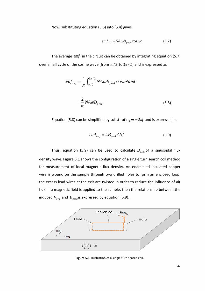
47

Now, substituting equation (5.6) into (5.4) gives

tBNAemf peak cos (5.7)

The average emf in the circuit can be obtained by integrating equation (5.7)

over a half cycle of the cosine wave (from 2/ to 2/3 ) and is expressed as

2/3

2/cos

1

ttdBNAemf peakavg

peakBNA

2 (5.8)

Equation (5.8) can be simplified by substituting f 2 and is expressed as

ANfBemf peakavg 4 (5.9)

Thus, equation (5.9) can be used to calculate peakB of a sinusoidal flux

density wave. Figure 5.1 shows the configuration of a single turn search coil method

for measurement of local magnetic flux density. An enamelled insulated copper

wire is wound on the sample through two drilled holes to form an enclosed loop;

the excess lead wires at the exit are twisted in order to reduce the influence of air

flux. If a magnetic field is applied to the sample, then the relationship between the

induced avgV and peakB is expressed by equation (5.9).

Figure 5.1 Illustration of a single turn search coil.

48

Some possible sources of error in the search coil method are outlined below:

The influence of air flux [5.3]. An air gap could be enclosed when winding

the coil on the sample; this could result a higher measurement.

The effect of stress on local magnetic structure. Drilling-induced residual

stress and magnetostatic energy can cause reconfiguration of local magnetic

domain structures. An example of how domain structure is changed after

drilling is shown in figure 5.2. Distorted domain pattern is observed around

the edges of the hole, they indicate the damaged region caused by drilling.

Domain reconfiguration could cause a slight change in the magnetisation

process, thus leading to an inconsistent flux density measurement before

and after drill search coil holes.

Figure 5.2 Distorted magnetic domain pattern around drilled hole in grain oriented

electrical steel [5.4].

Error due to the measurement of the area enclosed by the search coil. Care

must be taken when calculating the area of the search coil to use in

equation 5.9. It is shown in figure 5.3 that a deformed flux path is predicted

near the search coil holes. Total flux enclosed by the coil is equivalent to the

flux shown in the effective area. As a result, the effective distance should be

taken into calculation of the search coil enclose area; that is, the distance

49

between the two centres of the drill holes multiplies the thickness of the

specimen.

Figure 5.3 Illustration of change in flux distribution before and after holes were drilled for installation of the search coil.

Short circuits due to burrs cut. The enamelled insulated wire is usually used

to prevent direct contact between the coil and the test specimen. However,

the insulation coating could be damaged by sharp burrs around the drill

holes and lead to a short circuit of the search coil.

Magnetic degradation caused by drilling. Drilled holes are occupied by air

whose magnetic permeability is much lower than that of the electrical steel

specimen. Localised intense application increases the volume fraction of air,

leading to a significant decline of the magnetic permeability of the test

specimen.

Some of the drawbacks discussed above could be minimised by reducing the

hole diameter to reduce the damaged region, covering the burrs with non-magnetic

coating (e.g. nail varnish) to prevent short circuits, and stress relief annealing to

remove some of the drill induced stress.

50

Some history and previous related investigations of the search coil method

are summarised below:

The search coil method for the measurement of local flux density in

electrical steels was first developed by Brailsford and Mazza [5.5]. They drilled holes

in a steel specimen and coated the sides with insulation material. A single turn coil

was wrapped through the holes and flux density was determined from the induced

voltage signal.

Later, Mapps [5.4] studied the effect of drill holes on local domain

structures of grain oriented steels. Distorted domain patterns were observed

around all drill holes, and he found that the holes that were drilled on grain

boundaries has less effect on domain configuration compared to those within the

grains.

Tumanski [5.6] and [5.7] carried out an investigation to study the effect of

drilling on the magnetic properties of electrical steels. His experimental results

showed that annealing cannot completely remove the damage caused by drilling as

closure domains were created around the holes to reduce flux leakage and the

remaining plastic stress will continue to cause change in domain structure as seen

in figure 5.2.

Zurek [5.8] analysed the effect of twisting lead wire on the accuracy of

search coil measurements. A 0.1 mm diameter enamelled wire was used for making

search coil in the investigation; the experimental results showed that a tight and

uniformly twisted lead wire can reduce the influence of stray fields by up to 60% on

flux density measurement compared to a loosely twisted wire.

5.1.2 Needle probe method

The needle probe method detects magnetic flux density by means of

measuring the electrical potential difference between two points on one surface of

a specimen where needles are applied as shown in figure 5.4.

51

Two assumptions must be made in order to satisfy the needle probe theory

which shows that the potential difference 𝑉𝑁 (as shown in figure 5.4) between the

needles is in proportion to the rate of change of flux in the area 12341. Firstly, it is

assumed that the magnetic flux density is symmetrically distributed with respect to

the centre line (dash line) of the cross sectional area of the test specimen shown in

figure 5.4; thus, an equal amount of flux travels through the top and bottom

sections of the specimen. Secondly, it is assumed that the ratio of the needle

separation spacing to the specimen thickness is high so that the thickness of the

specimen can be neglected when compared to the needle separation spacing.

Figure 5.4 Illustration of needle probe method.

From the Maxwell-Faraday equation, the electric field created by a changing

magnetic field within the area 12341 in figure 5.4 can be written as the closed loop

integral shown below

Sddt

BdldE

SC

(5.10)

where C denotes the closed contour 12341, E denotes the induced electric field

intensity and S denotes the area of the contour. By considering the components of

the induced electrical field, equation (5.10) can be re-written as

Sddt

BdVVVV

S

41342312 (5.11)

52

If the flux is distributed uniformly within the contour, then 4123 VV and

04123 VV

since they have opposite signs. 034 V

since it is at the central line of

the symmetrical shape, so equation (5.11) can be simplified as

Sddt

BdV

S

12 (5.12)

Because 2/AS . Now, combining equation (5.12) with (5.8) gives the

following equation for the average voltage between needles 12V :

AfBV peak212 (5.13)

For a single-turn search coil, the voltage induced in the coil is expressed as

AfBV peak4 (5.14)

Thus, from a computational perspective, the needle probe method is also

considered as a half turn search coil. No holes are necessary so several of the

drawbacks of the search coil method are not present and also the technique is less

time-consuming than the search coil method.

However, the technique is susceptible to various errors [5.3][5.8][5.9] and

[5.10] that may reduce the accuracy of the measurement, which are outlined below:

The influence of air flux. Like the search coil method, the needle probe also

suffers from the interference of air flux that is enclosed by the lead wire and

needles. The important difference is that the enclosed air flux will lead to

reduction of flux density measurement rather than increasing it.

Systematic errors due to the remaining components of vertical electric fields

[5.9]. The theory assumes that 4123 VV and 04123 VV

. In practice, the

test material probably contains different degrees of local anisotropy which

53

leads to 4123 VV . Due to the second assumption made in the needle

technique, this error is restricted to a minimum by assuming the component

of the vertical electric field is neglected compared to the main horizontal

electric field.

Systematic errors due to the edge effect [5.10]. The application of the

needle technique could fail at the specimen’s near edge, where 34V (the

centre line) is not zero. Thus, needle measurement must be conducted at a

distance away from the edges of the specimen, usually a distance of 1/2

specimen thickness is recommended [5.11].

The effect of the inhomogeneous nature of the material. It is important for

the test material to be homogeneous throughout its thickness. The method

assumes the same flux density should be present in the top and bottom

sections of the test specimen; thus, the needle measurement obtained over

one surface can be used to represent the flux density of the entire cross

sectional area. However, the test materials may contain different degrees of

inhomogeneity due to the manufacturing process and distribution of

inclusions.

The effect of insulation coating on needle measurement. The needle

technique has been used for measurement of flux density of electrical steels

without removing the insulation coating. Users apply sharp needles to

pierce through the insulation and make an electrical contact with the

specimen underneath. Poor contact may occur and will lead to a possible

loss of the needle signals.

There are some useful methods which can be used to scale down the

influence of these errors on needle measurement. Examples include increasing the

ratio between needle separation spacing and specimen thickness, removing the

insulation coating of test specimens and avoiding edge measurement by placing the

probe at least ½ sample thickness away from the edges.

54

Some history and previous related investigations of the needle probe

method are summarised below:

In 1949, Werner proposed a method for the measurement of magnetic flux

density by means of measuring the potential difference between two needles

placed on the test sample (cited [5.3] and [5.8]). Later, the method was patented

separately by Czeija [5.12] and Stauffer [5.13].

The earliest work regarding the measurement of magnetic flux density in

electrical steel samples using the needle probe technique was carried out by

Tompkins [5.14]. In his experiment, local magnetic properties of a single sheet

sample were measured by a probe which consisted of a pair of metal needles and a

magnetic potentiometer (Chattock coil) element as shown in figure 5.5. The design

allowed flux density and magnetising field to be measured locally, and the

hysteresis loop of the test point could be plotted from flux density and magnetising

field signals. In addition, power loss could be derived by integrating the product of

BdH. The resolution of the probe was reported at 25.4 x 50.8 mm2.

Figure 5.5 Illustration of the comparator probe [5.14].

Wilkins [5.15] set up an experiment to compare the needle probe technique

with the search coil method on strips of grain-oriented electrical steels. A pair of

brass needles was used for the elimination of the extraneous signals and was

55

placed, in turn, next to the 0.25 mm diameter search coil holes which were 6.35

mm apart. A single turn coil was wound through the holes to measure the flux

density of the same region. The result showed that the output signals of both

techniques were agreed well with each other across all measurement points.

Brix [5.16] designed an instrument for the measurement of rotational

magnetisation, in which the flux density was detected utilising the needle probe

technique. Probe needles were spring loaded to ensure successive contact during

magnetisation. A similar experiment [5.17] was conducted using the search coil

method; the flux densities at the identical locations agreed well with the

measurements obtained using the needle probe technique.

Senda [5.18] studied the effect of the experimental set-up on the accuracy

of the needle probe technique. Two tungsten needles with 50 μm tip diameters

were placed 10 mm apart on 0.23 mm thick electrical steel specimen. The first

experiment was conducted to investigate the effect of loading stress on the

measurement. The results showed that the loading effect on local flux density value

was less than 0.2 % for a 50 g / needle loading and was less than 1.5 % for loading

which does not exceed 300 g / needle. The second experiment was conducted to

investigate the influence of the symmetry of the in-plane eddy current on the

needle probe measurement. The test specimen was magnetised in turn by two

types of magnetising systems shown in figure 5.6. The type A configuration was one

side contact and the type B configuration was two sides contact. In type A

configuration, a maximum difference of 13 % was measured between

measurements obtained using needle probe and search coil at induction of 1.7 T.

Whereas in type B configuration, the maximum difference was only 0.9 %.

The differences in the type A configuration are caused by the non-

symmetrical distribution of the eddy current and are explained by Nakata [5.19].

For the single-sided contact magnetising system, the generation of in-plane eddy

current distorts the profile of the surface electric field and affects the accuracy of

the needle probe measurement. However, for the double-sided contact

magnetising system, the in-plane eddy currents generated on the two sides of the

56

specimen should cancel each other out since the rotation of the current are in the

opposite directions.

Figure 5.6 Illustration of two different types of yoke configuration [5.18].

Loisos [5.9] carried out a critical evaluation of local magnetic flux density

measurement methods. In the investigation, three techniques namely search coil,

needle probe and modified needle probe were compared using a 0.5 mm thick non-

oriented specimen, magnetised at 50 Hz and peak flux density range from 0.6 T to

1.4 T. The authors described the so called modified needle probe method which is

demonstrated in figure 5.7. The method requires very precise needle positioning

control; the two pairs of needles must be placed at identical locations on both sides

of the specimen. Voltage VA is induced by flux travelling in the area S2 and voltage

VB is induced by flux travelling in the area (S1 + S2). Therefore, the overall voltage

induced in the measurement area BAA’B’ equals VB – VA and is equivalent to the

voltage induced in a one turn search coil placed on the same area. During the

experiment, the needle-separation-distance of both the needle probe method and

the modified needle probe method were set to the same 25 mm, 11.5 mm and 4

mm. Single turn enamelled wire search coils were place at identical locations

wound through the pre-drilled 0.5 mm diameter holes next to each needle point.

Errors due to the vertical field in the needle probe method were studied by

analysing the ratio between the needle separation and the specimen thickness. The

highest percentage error occurred in the conventional needle probe measurement

where the needle-separation distance was the lowest. This was found to be about

12.5 % for the 4 mm needle-separation and it reduced to 2 % for the 25 mm needle-

separation. Whereas the modified needle probe showed less influence on the

57

vertical field since VA and VB cancelled out each other, a higher spread of

measurements was observed.

The author stated that, for the considerable less homogenised grain

oriented steel specimens, the use of the modified needle probe can provide

improved accuracy. However, its application is often restricted because of the

wiring connection and the demand for a precise positioning system.

Figure 5.7 Illustration of the modified needle probe technique [5.9].

The latest use of the needle probe technique for flux density measurement

was carried out by Crevecoeur [5.20]. A non-destructive investigation of the effect

of cutting on the magnetic hysteresis properties of electrical steel specimens was

carried out. The experimental technique applies a needle probe sensor that was

described in the authors’ earlier work [5.21] and is shown in figure 5.8 (a). The path

of the eddy current is distorted as it approaches the cut edge as shown in figure 5.8

(b), the area Sa ≠ Sb ≠ Sc. Therefore, in order to obtain accurate results, Sb and Sc

must be calculated numerically using the method described in [5.20] and [5.21].

The specimen under test was a laser cut non-oriented steel sheet, the test probe

was made of 15 needles arranged transversely along the width of the sheet, the

probe was placed with one end at the cut edge (degraded region) and the other

end close to the centre of the sheet (non degraded region). The result showed that

needle signals collected at the cut edge were higher than in the centre because the

induction area S is larger at the edge. In addition, at the centre of the sheet where it

was considered to be deformation free, the needle signal was found to be smaller.

58

Figure 5.8 (a) Needle sensors. (b) Illustration of eddy current flow at sample edge and surfaces of

induced voltage covered by needle sensors [5.20].

5.2 Local magnetic field measurement techniques

The magnetic field on the surface of electrical steel can be measured by a

variety of techniques. In this section, two commonly used techniques, known as the

air-cored induction coil sensor and the Hall Effect sensor, are discussed and

commented on in order to help the selection of a suitable technique for this

investigation.

5.2.1 Air-cored induction coil sensor

The air-cored induction coil is also known as the H-coil. It is one of the

simplest methods for an accurate measurement of the surface magnetic field of an

electrical steel specimen [5.22]. The principle of the method is based on Faraday’s

law which is described in section 5.1.1.

A typical H-coil sensor is made by winding an on a non-magnetic former

having 1r . The induced emf in the coil is proportional to the time varying

magnetic flux density dtdB / since there is a linear relation between B and H in the

air, from equation 5.3 the induced emf in the coil can be expressed as

dt

dHNAemf 0 (5.14)

where N is the number of identical turns on the H-coil. Thus, rearranging the above

equation and giving the magnetic field H inside the coil as

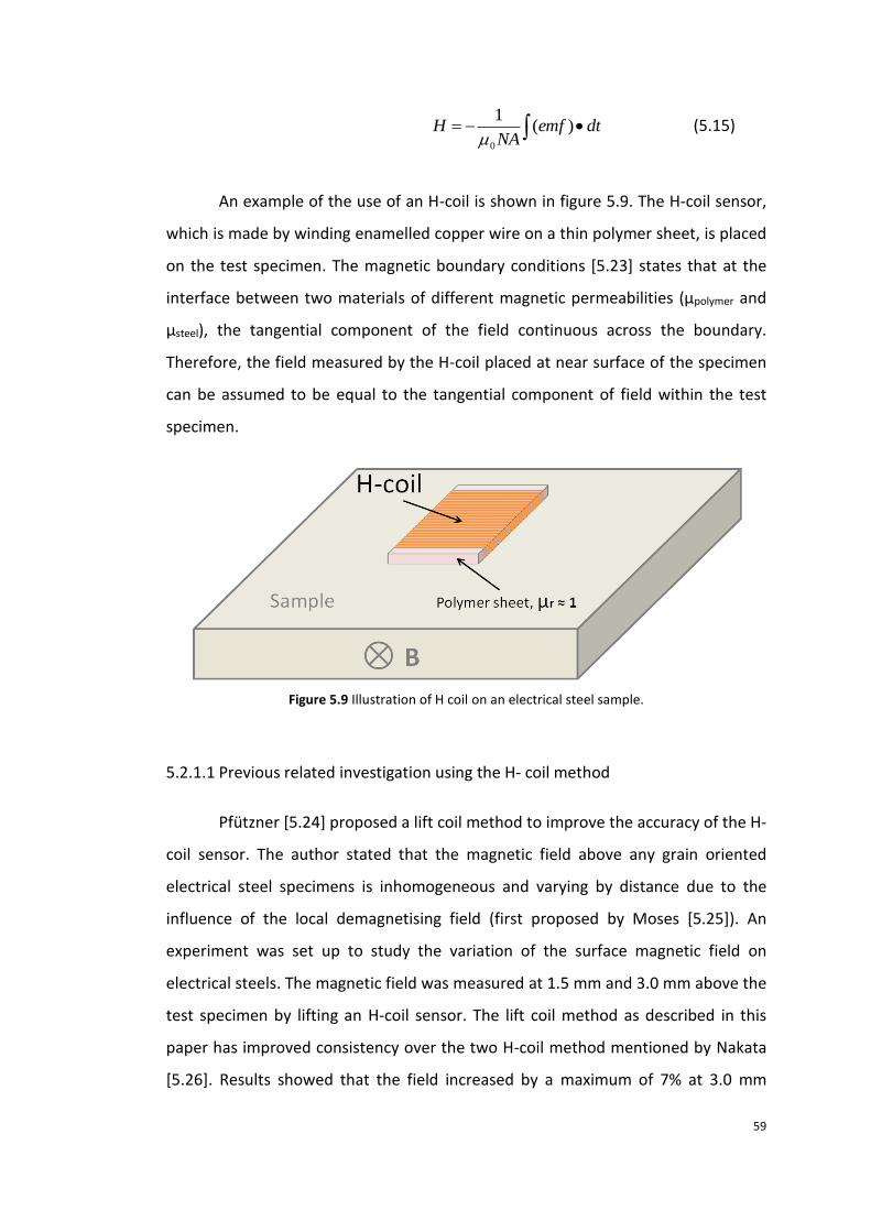
59

dtemfNA

H )(1

0 (5.15)

An example of the use of an H-coil is shown in figure 5.9. The H-coil sensor,

which is made by winding enamelled copper wire on a thin polymer sheet, is placed

on the test specimen. The magnetic boundary conditions [5.23] states that at the

interface between two materials of different magnetic permeabilities (μpolymer and

μsteel), the tangential component of the field continuous across the boundary.

Therefore, the field measured by the H-coil placed at near surface of the specimen

can be assumed to be equal to the tangential component of field within the test

specimen.

Figure 5.9 Illustration of H coil on an electrical steel sample.

5.2.1.1 Previous related investigation using the H- coil method

Pfützner [5.24] proposed a lift coil method to improve the accuracy of the H-

coil sensor. The author stated that the magnetic field above any grain oriented

electrical steel specimens is inhomogeneous and varying by distance due to the

influence of the local demagnetising field (first proposed by Moses [5.25]). An

experiment was set up to study the variation of the surface magnetic field on

electrical steels. The magnetic field was measured at 1.5 mm and 3.0 mm above the

test specimen by lifting an H-coil sensor. The lift coil method as described in this

paper has improved consistency over the two H-coil method mentioned by Nakata

[5.26]. Results showed that the field increased by a maximum of 7% at 3.0 mm

60

compared to that measured at 1.5 mm. This agreed with the proposal [5.27] made

earlier by the authors. In addition, by using linear mathematical extrapolation, the

lift coil method can be using for the calculation of the magnetic field within any test

specimen.

Later, Tumanski [5.28] also studied the variation of the magnetic field as a

function of distance above a grain oriented electrical steel strip. His study consists

of both numerical and experimental investigations, in which the experimental result

was obtained through averaging local field strength using a magnetovision map

[5.29]. The test strip were magnetised in turn by single yoke and double yoke

systems. Figure 5.10 shows the distribution of the magnetic field as a function of

distance above the test specimen. The double yoke system for magnetising

specimens was strongly recommended by the authors (as discussed in 5.1.2). For

the double yoke system, the authors explained the sudden increase in magnetic

field strength at the near surface was caused by the distortion of a stray field from

domains and grain boundaries. As a result, when the double yoke construction is

used for magnetising the specimen, the field sensor should be placed at

approximately 1 mm above the test specimen to avoid the influence of the stray

field. (No further explanation was given by the authors on the significance of the

effect).

Figure 5.10 The dependence of the magnetic field above the sample surface versus distance from

the sample magnetised by single yoke system 1C and double yoke system 2C [5.28].

61

5.2.2 Hall effect sensor

The Hall Effect sensor measures the magnetic field by applying the Hall

Effect which was discovered by Edwin Herbert Hall In 1879. The Hall Effect states

that when a plane of a current carrying conductor is placed perpendicular to the

direction of a magnetic field, an electric potential 𝑉𝐻 (as shown in figure 5.11) will

arise in the plane of the current carrying conductor and perpendicular to the

direction of the current. Figure 5.11 displays the configuration of the vectors of the

Hall Effect.

Figure 5.11 Illustration of the Hall Effect.

A typical Hall Effect sensor consists of a rectangular semiconducting plate

with two pairs of electrical contacts at right angle to each other [5.22]. During the

measurement, a DC current is conducted via one pair of the contacts. If the

magnetic field perpendicular to the semiconducting plate is not zero, then the

movement of electrons is distorted (left hand rule and Lorentz force law). As a

result, an electrical potential is formed transverse to the current direction. The

induced Hall voltage is proportional to the product of magnetic field strength and

the current.

To improve the sensor sensitivity, Hall sensors made of thin plate of low-

carrier-concentration semiconductor are usually preferred since the Hall voltage is

inversely proportional to the thickness and carrier concentration of the plate.

62

Conductors such as Cu may be used, but compared with semiconductors such as

indium arsenide (InAs), Cu has lower Hall coefficients. In addition, InAs has low

temperature sensitivity therefore is less influenced by the surrounding environment.

In terms of the fabrication, modern Hall sensors are made of integrated

circuits [5.30] for reduced capital cost and improved product quality. Commercial

sensors are relatively cheap compared with H-coil sensors and their geometries and

size are designed for specific applications.

5.2.2.1 Previous related investigation using Hall sensor

The earliest examples utilising the Hall sensor for magnetic field

measurement on a steel sample were conducted by Evans and Peeve [5.31]. In the

study, by assuming the magnetising field distributes uniformly across the entire

specimen, the magnetic field applied to the specimen was measured by a Hall Effect

sensor which was placed in the pre-drilled hole in the test specimen.

Moses [5.32] conducted an experiment to study the distribution of the

surface field on a grain oriented steel sample using a Hall effect integrated circuit

sensor. The sensor was calibrated in a uniform magnetic field, which was created by

a DC current carrying solenoid, a sensor sensitivity of 0.03 mV/Am-1 was found. In

the measurement, the magnetic field of the specimen was sensed by placing the

Hall Effect sensor 0.25 mm above the specimen.

Stupakov [5.33] measured surface field strength of an electrical steel sample

using Hall Effect sensors with build in high-gain amplifier. Such sensors allow a

localised magnetic field to be measured at a very low strength. Figure 5.12 shows

the B-H loop obtained from the Hall sensor measurement. The author explained

that the distortion appearing on the loop is due to the thermal noise which

influences the stability of the sensors. The presence of the thermal distortion can

directly affect the accuracy of the measurement and must be improved. One of the

more useful methods for the removal of the thermal distortion seen on the B-H

loop was by averaging over a high number of cycles. An example of a noise

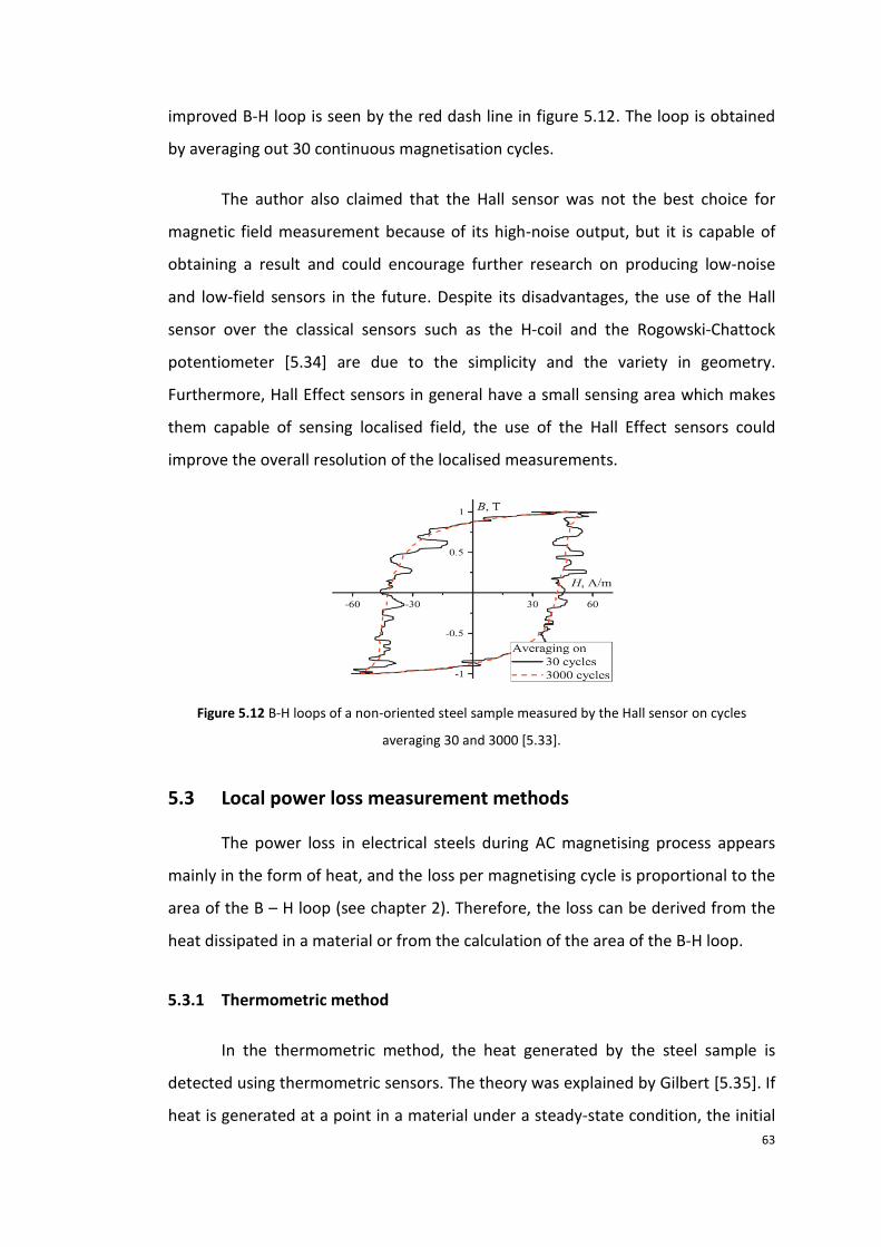
63

improved B-H loop is seen by the red dash line in figure 5.12. The loop is obtained

by averaging out 30 continuous magnetisation cycles.

The author also claimed that the Hall sensor was not the best choice for

magnetic field measurement because of its high-noise output, but it is capable of

obtaining a result and could encourage further research on producing low-noise

and low-field sensors in the future. Despite its disadvantages, the use of the Hall

sensor over the classical sensors such as the H-coil and the Rogowski-Chattock

potentiometer [5.34] are due to the simplicity and the variety in geometry.

Furthermore, Hall Effect sensors in general have a small sensing area which makes

them capable of sensing localised field, the use of the Hall Effect sensors could

improve the overall resolution of the localised measurements.

Figure 5.12 B-H loops of a non-oriented steel sample measured by the Hall sensor on cycles

averaging 30 and 3000 [5.33].

5.3 Local power loss measurement methods

The power loss in electrical steels during AC magnetising process appears

mainly in the form of heat, and the loss per magnetising cycle is proportional to the

area of the B – H loop (see chapter 2). Therefore, the loss can be derived from the

heat dissipated in a material or from the calculation of the area of the B-H loop.

5.3.1 Thermometric method

In the thermometric method, the heat generated by the steel sample is

detected using thermometric sensors. The theory was explained by Gilbert [5.35]. If

heat is generated at a point in a material under a steady-state condition, the initial

64

rate of the rise of the temperature at this point is proportional to the generated

heat. Based on this theory, the power loss P of electrical steel can be expressed as

[5.36]

])([)(

0TtTkdt

tdTcp extp (5.16)

where 𝑃 is the thermal power loss has units of Joules (J), pC is the specific heat of

the test sample and has units of Joules per Kilogram per Kelvin (J/KgK) and dT is the

change in temperature of the measured point over a period of dt seconds. 𝐾𝑒𝑥𝑡 is

the heat transmission coefficient (to the surroundings) has unit of Watts per

kilogram per Kelvin (W/kgK), and T0 is initial temperature of material and

surrounding before being magnetised.

For power loss localised measurements, Gilbert [5.35] suggested that the

initial time taken to measure the rate of the temperature rise should be less than

10 seconds, above which the method rate of rise of temperature becomes non-

uniform due to heat diffusion. This time should vary to some extent depend on

thermal diffusion rate of the material.

Moses [5.38] measured power loss distribution in a stator core using

thermistors. The initial temperature rise was recorded for a period of 20 seconds,

and the experimental error was estimated to about ±8 %.

Hamzehbahmani [5.39] compared local power loss measurement

techniques and developed a system for loss measurement based on the

thermometric method; the author declared that their system was mostly suitable

for the measurement of local losses at regions where distorted flux was found (i.e.

around bolt holes and near burr regions), where the techniques for the

measurement of localised magnetic field and flux density may fail.

However, the thermometric method was reported to have poor accuracy at

low flux density. The method suffers from low signal to noise ratio. In addition, the

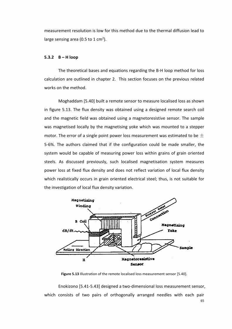
65

measurement resolution is low for this method due to the thermal diffusion lead to

large sensing area (0.5 to 1 cm2).

5.3.2 B – H loop

The theoretical bases and equations regarding the B-H loop method for loss

calculation are outlined in chapter 2. This section focuses on the previous related

works on the method.

Moghaddam [5.40] built a remote sensor to measure localised loss as shown

in figure 5.13. The flux density was obtained using a designed remote search coil

and the magnetic field was obtained using a magnetoresistive sensor. The sample

was magnetised locally by the magnetising yoke which was mounted to a stepper

motor. The error of a single point power loss measurement was estimated to be ±

5-6%. The authors claimed that if the configuration could be made smaller, the

system would be capable of measuring power loss within grains of grain oriented

steels. As discussed previously, such localised magnetisation system measures

power loss at fixed flux density and does not reflect variation of local flux density

which realistically occurs in grain oriented electrical steel; thus, is not suitable for

the investigation of local flux density variation.

Figure 5.13 Illustration of the remote localised loss measurement sensor [5.40].

Enokizono [5.41-5.43] designed a two-dimensional loss measurement sensor,

which consists of two pairs of orthogonally arranged needles with each pair

66

separated 15 mm apart and a 10 x 10 mm orthogonal H coil site in between the

needles. The needles were loaded with springs to protect the specimens from

contact damage during the magnetising vibration.

Senda [5.17] and [5.44] measured local power loss using a self-made probe

shown in figure 5.14. A pair of tungsten needles 10 mm apart were arranged

transverse to the sample rolling direction, and a Hall Effect sensor was placed

between the needles.

Figure 5.14 Illustration of the probe for local loss measurement [5.44].

In this investigation, a local loss measurement probe which consists of a pair

of needles and an integrated Hall element was constructed for the measurement of

local loss on grain oriented steel specimens. The output signals of B(t) and H(t) are

substituted into equation 2.13 (see chapter 2) for the calculation of power loss.

Further details regarding the signal processing are outlined in chapter 6.

67

References [5.1] D. Halliday, R. Resnick and K. S. Krane, “Physics”, Wiley, New York, 4th

Edition, vol. 2, pp. 784 – 785, (1992).

[5.2] W. H. Hayt, “Engineering electromagnetics”, McGraw-Hill, New York, 5th

edition, pp. 312 – 313, (1989).

[5.3] G. Loisos, “Novel flux density measurement methods of examining the

influence of cutting on magnetic properties of electrical steels”, Ph.D. thesis,

Cardiff University, (2002).

[5.4] D.J. Mapps, “Stress, power loss and domain structure in grain oriented

silicon iron”, Ph.D. Thesis, University of Cardiff, (1969).

[5.5] F. Brailsford and V. R. Mazza, “Magnetic flux distribution in transformer

laminations”, Journal of the Institution of Electrical Engineers, vol. 8, pp. 552

– 553, (1962).

[5.6] S. Tumanski, “The experimental verification of the condition of the magnetic

material caused by different technological processes”, Journal of Magnetism

and Magnetic Materials, vol. 215 – 216, pp. 749 – 752, (2000).

[5.7] S. Tumanski and M. Stabrowski, “The magnetovision method as a tool to

investigate the quality of electrical steel”, Meas. Sci. Technol, vol. 9, pp. 488

– 495, (1998).

[5.8] S. Zurek, T. Meydan and A. J. Moses, “Analysis of twisting of search coil leads

as a method reducing the influence of stray fields on accuracy of magnetic

measurements”, Sensors and Actuators, vol. 142, pp. 569 – 573, (2008).

[5.9] G. Loisos and A. J. Moses, “Critical evaluation and limitations of localized flux

density measurements in electrical steels”, IEEE Transactions on Magnetics,

vol. 37, pp. 2755 – 2757, (2001).

[5.10] H. Pfützner and G. Krismanić, “The needle method for induction tests:

sources of error”, IEEE Transactions on Magnetics, vol. 40, pp. 1610 – 1616,

(2004).

[5.11] M. D. Wulf, L, Dupre, D. Makaveev and J. Melkebeek, “Needle-probe

techniques for local magnetic flux measurements”, Journal of Applied

Physics, vol 93, pp. 8271 – 8273, (2003).

68

[5.12] E. Czeija and R. Zawischa, Austrian Patent 180990, (1955).

[5.13] L. H. Stauffer, U.S. Patent 2828467, (1958).

[5.14] R. E. Tompkins, L. H. Stauffer and A. Kaplan, “New magnetic core loss

comparator”, Journal of Applied Physics, vol. 29, pp. 502 – 503, (1958).

[5.15] F. J. Wilkins and A. E. Drake, “Measurement and interpretation of power

losses in electrical sheet steel”, Proc. IEE, vol. 112, pp. 771 – 785, (1965).

[5.16] W. Brix, K. A. Hempel and F. Schulte, “Improved method for the

investigation of the rotational magnetisation process in electrical steel

sheets”, IEEE Transactions on Magnetics, vol. 20, pp. 1708 – 1710, (1984).

[5.17] W. Brix, K. A. Hempel and W. Schroeder, “Method for the measurement of

rotational power loss and related properties in electrical steel sheets”, IEEE

Transactions on Magnetics, vol. 18, pp. 1469 – 1471, (1982).

[5.18] K. Senda, M. Ishida, K. Sato, M. Komatsubara and T. Yamaguchi, “Localised

magnetic properties in grain-oriented electrical steel measured by needle

probe method”, Electrical Engineering in Japan, vol. 126, pp. 942 – 949,

(1999).

[5.19] T. Nakata, K. Fujiwara, M. Nakano and T. Kayada, “Influence of yoke

construction on magnetic characteristics of single sheet tester”. Journal

Japanese Society Applied Magnetism, vol. 13, pp. 371 - , (1989).

[5.20] G. Crevecoeur, L. Dupre, L. Vandebossche and R. Van de Walle, “Local

identification of magnetic hysteresis properties near cutting edges of

electrical steel sheets”, IEEE Transactions on Magnetics, vol. 44, pp. 1010 –

1013, (2008).

[5.21] G. Crevecoeur, L. Duper, L. Vandenbossche and R. Van de Walle,

“Reconstruction of local magnetic properties of steels by needle probe

methods using space mapping techniques”, Journal of Applied Physics, vol.

99, pp. 08H905-1 – 08H905-3, (2006).

[5.22] R. Boll and K. J. Overshott, “Sensors: Volume 5 Magnetic Sensors”, VCH

Publishers Inc., New York, p.206, (1989).

[5.23] R. G. Carter, “Electromagnetism for electronic engineers”, 2nd edition,

Chapman & Hall, London, (1992).

69

[5.24] H. Pfützner and P. Schönhuber, “On the problem of the field detection for

single sheet testers”, IEEE Transactions on Magnetics, vol. 27, pp. 778 – 785,

(1991).

[5.25] A. J. Moses, “Recent advances in experimental methods for the investigation

of silicon iron”, Physica Scripta, vol. T24, pp. 49 – 53, (1988).

[5.26] T. Nakata, Y. Kawase and M. Nakano, “Improvement of measuring accuracy

of magnetic field strength in single sheet testers by using two H Coils”, IEEE

Transactions on Magnetics, vol. Mag-23, pp. 2596 – 2598, (1987).

[5.27] H. Pfützner, “Application of hall sensors in comparison to other methods of

field detection for investigations of electrical steel”, Z. el. Inform. U. En.

Techn., vol. 10, pp. 534 – 546, (1980).

[5.28] S. Tumanski, “A multi-coil sensor for tangential magnetic field

investigations”, Journal of Magnetism and Magnetic Materials, vol. 242 –

245, pp. 1153 – 1156, (2002).

[5.29] S. Tumanski and M. Stabrowski, “The magnetovison method as a tool to

investigate the quality of electrical steel”, Measurement Science and

Technology, vol. 9, pp. 488 – 495, (1998).

[5.30] S. A. Macintyre, “Magnetic Field Measurement”, CRC Press LLC, (1999).

[5.31] D. Evans and P. A. Reeve, “Automated high saturation B-H measuring

equipment”, IEEE Transactions on Magnetics, vol. 32, pp. 3045 – 3048,

(1996).

[5.32] A. J. Moses and S. N. Konadu, “Some effects of grain boundaries on the field

distribution on the surface of grain oriented electrical steels”, International

Journal of Applied Electromagnetics and Mechanics, vol. 13, pp. 339 – 342,

(2002).

[5.33] O. Stupakov, “System for controllable magnetic measurement with direct

field determination”, Journal of Magnetism and Magnetic Materials, vol. 324,

pp. 631 – 636, (2012).

[5.34] A. Khanlou, A. J. Moses, T. Meydan and P. Beckley, “A computerised on-line

power loss testing system for the steel industry, based on the RCP

70

compensation technique”, IEEE Transactions on Magnetics, vol. 31, pp. 3385

– 3387, (1995).

[5.35] A. J. Gilbert, “A method of measuring loss distribution in electrical

machines”, The Institution of Electrical Engineers, vol. 108, pp. 239-244,

(1961).

[5.36] H. Hamzehbahmani, A. J. Moses and F. J. Anayi, “Opportunities and

precautions in measurement of power loss in electrical steel laminations

using the initial rate of rise of temperature method”, IEEE Transactions on

Magnetics, vol. 49, pp. 1264 – 1273, (2013).

[5.37] B. D. Ismail, “Investigation of flux and loss distribution in transformer cores

assembled from amorphous powercore material”, Ph.D. thesis, University of

Wales College Cardiff, (1991).

[5.38] A. J. Moses and N. Tutkun, “Localised losses in stator laminations of an

induction motor under PWM excitation”, Journal of Materials Processing

Technology, vol. 161, pp. 79 – 82, (2005).

[5.39] H. hamzehbahmani, A. J. Moses and F. J. Anayi. “Opportunities and

precautions in measurement of power loss in electrical steel laminations

using the initial rate of rise of temperature method”, IEEE Transactions on

Magnetics, vol. 49, pp. 1264 – 1273, (2013).

[5.40] A. J. Moghaddam and A. J. Moses, “Localised power loss measurement using

remote sensors”, IEEE Transactions on Magnetics, vol. 29, pp. 2998 – 3000,

(1993).

[5.41] M. Enokizono, I. Tanabe and T. Kubota. “Localized distribution of two-

dimensional magnetic properties and magnetic domain observation”,

Journal of Magnetism and Magnetic Mmaterials, vol. 196 – 197, pp. 338 –

340, (1999).

[5.42] M. Enokizono, M. Morikawa, K. Kawamura and J. Sievert. “Distribution of

two-dimensional magnetic properties in three-phase induction motor model

core”, IEEE Transactions on Magnetics, vol. 32, pp. 4989 – 4991, (1996).

[5.43] T. Kanada, M. Enokizono, K. Kawamura and J. D. Sievert. “Distributions on

localised iron loss of three-phase amorphous transformer model core by

71

using two-dimensional magnetic sensor”, IEEE Transactions on Magnetics,

vol. 32, pp. 4797 – 4799, (1996).

[5.44] K. Senda, M. Kurosawa, M. Ishida, M. Komatsubara and T. Yamaguchi. “Local

magnetic properties in grain-oriented electrical steel measured by the

modified needle probe method”, Journal of Magnetism and Magnetic

Materials, vol. 215 – 216, pp. 136 – 139, (2000).

72

Chapter 6

Experimental Apparatus

This chapter describes the apparatus used for observation of magnetic

domain and the local loss measurement system used for the measurement of

localised flux density, magnetic field and power loss of grain oriented electrical

steels. The method for evaluation of uncertainty in the measurements is also

outlined in this chapter.

6.1 Apparatus for the observation of magnetic domains of electrical

steel samples.

6.1.1 Static domain imaging using magnetic domain viewer

A magnetic domain viewer based on the modified Bitter technique outlined

in chapter 4 was used in this investigation for the study of grain structure and the

static magnetic domain pattern of electrical steel specimens.

Figure 6.1 shows the magnetic domain viewer with 90 mm diameter

observation area which was used in this investigation. This domain viewer consists

of a circular-shaped clear plastic body, a build-in magnetic coil, a Bitter fluid

injection port, lead wiring to an external DC power supply, a plastic film membrane

and the Bitter fluid (a mixture of fine Fe2O3 particles, soap and distilled water).

73

The coil is wound along the ring-shaped groove of the viewer body as seen

in figure 6.2. An external DC power supply is connected to the coil for the

generation of a magnetic field of approximately 2.2 KAm-1 [6.1] perpendicular to the

surface of the test specimen. Grain oriented electrical steel is rarely perfectly

oriented; a small tilt angle is expected to form during the coil annealing process

(also known as the secondary recrystallisation). Therefore, as shown in figure 6.2,

magnetisation of one type domain (e.g. N-S domain) will rotate towards the surface

plane and the other type domain (e.g. S-N domain) will rotate away from the

surface plane. As a result, stray field profile of the viewing specimen is modified,

more ferromagnetic particles are attracted by the S-N domains and less is attracted

by the N-S domain. Thus, a black and white contrast is developed by the black

ferromagnetic particles and the white background membrane, which indicates the

anti-parallel bar domains of the grain oriented electrical steel.

Figure 6.1 Photograph of the magnetic domain viewer which was used in this investigation.

Figure 6.2 Cross-section illustration showing the working principle of the magnetic domain viewer.

74

Application of the external field improves the Bitter pattern contrast. In

addition, the contrast of the image was further boosted through the use of

Photoshop Pro image editing software.

6.1.2 Dynamic domain imaging using Magneto-optical Kerr microscope.

Figure 6.3 shows the low magnification Kerr microscopy system used in this

investigation. The system consists of three separate sections, the light source,

magnetising and collection.

The light source section – this consists of a Schott KL1500 LCD light source,

an optical cable and a plane polariser.

The magnetising section – this consists of an adjustable sample stage, a coil

wound C-shape yoke of 20 mm pole separation spacing, a TTi 40 MHz arbitrary

wave generator and an Amcron DC 300 A amplifier.

The collection section – this consists of a low magnification lens, a Kerr

Effect analyser, a Photron fastcam MC1 camera and DpxView Pro camera software

installed prior in the PC. Specification of the camera is shown in table 6.1.

Dimensions (camera head)

Weight (head)

Sensor type Resolution Frame rate Recording memory

Trigger method

35 (W) x 35 (H) x 33.3 (D) mm

90 g CMOS 512 x 512

pixels

2,000 fps (up to

10,000 with reduced

resolution)

2 GB Start,

centre and end

Table 6.1 Manufacture specification of the Photon fastcam MC1 high speed camera [6.2].

75

Figure 6.3 Photograph of the low magnification Kerr microscope.

A high intensity light beam was produced by the Schott KL1500 LCD light

source, which was then focused and directed to the plane polariser using the optical

cable shown on the left side of figure 6.3. The beam was then passed through the

polariser to make polarised light which illuminates the test specimen. The reflected

beam with a polarisation angle of +θk or -θk (outlined in chapter 4.4) travelled

through the magnification lens and the analyser to form the Kerr contrast which

was captured by the camera. During the observation, the angle of

incidence/reflection was adjusted to approximately 50o to obtain optimum Kerr

contrast [6.3].

To observe domain wall motion, a magnetic field waveform was produced by

the TTi 40 MHz arbitrary wave generator, which was then fed into the Amcron DC

300A amplifier to gain the desired field strength. The magnetising field was applied

to the test specimen through the coil wound C-shape yoke which sat underneath of

the specimen.

76

6.2 Introduction to the system for the measurement of the local

magnetic properties of the single strip electrical steel samples.

A computer-controlled AC magnetising and scanning loss measurement

system was developed in the Wolfson Centre for Magnetics. The system is able to

apply a global AC magnetising field to a single strip, Epstein size electrical steel

specimen and measure its localised magnetic field, flux density and power loss in an

area of up to 30 x 70 mm in the middle of the strip at a raster scanning resolution of

up to 0.1 mm. It comprises three sub-systems: magnetising, measurement and

positioning. The magnetising system magnetises the test sample at set

magnetisation conditions, the measurement system is used to measure the globally

induced magnetic flux density as well as detecting the localised magnetic flux

density, magnetising field and power loss at the point where the sensor is located,

and the positioning system is used to move the sensor between the measurement

points.

Figure 6.4 shows how information is inter-exchanged in order to complete

the measurement process. The positioning system communicates with the

measurement system to identify whether the measurement has been finished and

ready to relocate the sensor to the next measurement point. The measurement

system feeds back the information regarding the flux density waveform to the

magnetising system in order to control and accurately maintain the magnetisation

conditions within the set tolerance (outlined in 6.2.1) so that each measurement is

recorded at the same induced global magnetisation.

Figure 6.4 Schematic diagram of computer-controlled AC magnetising and scanning measurement

system.

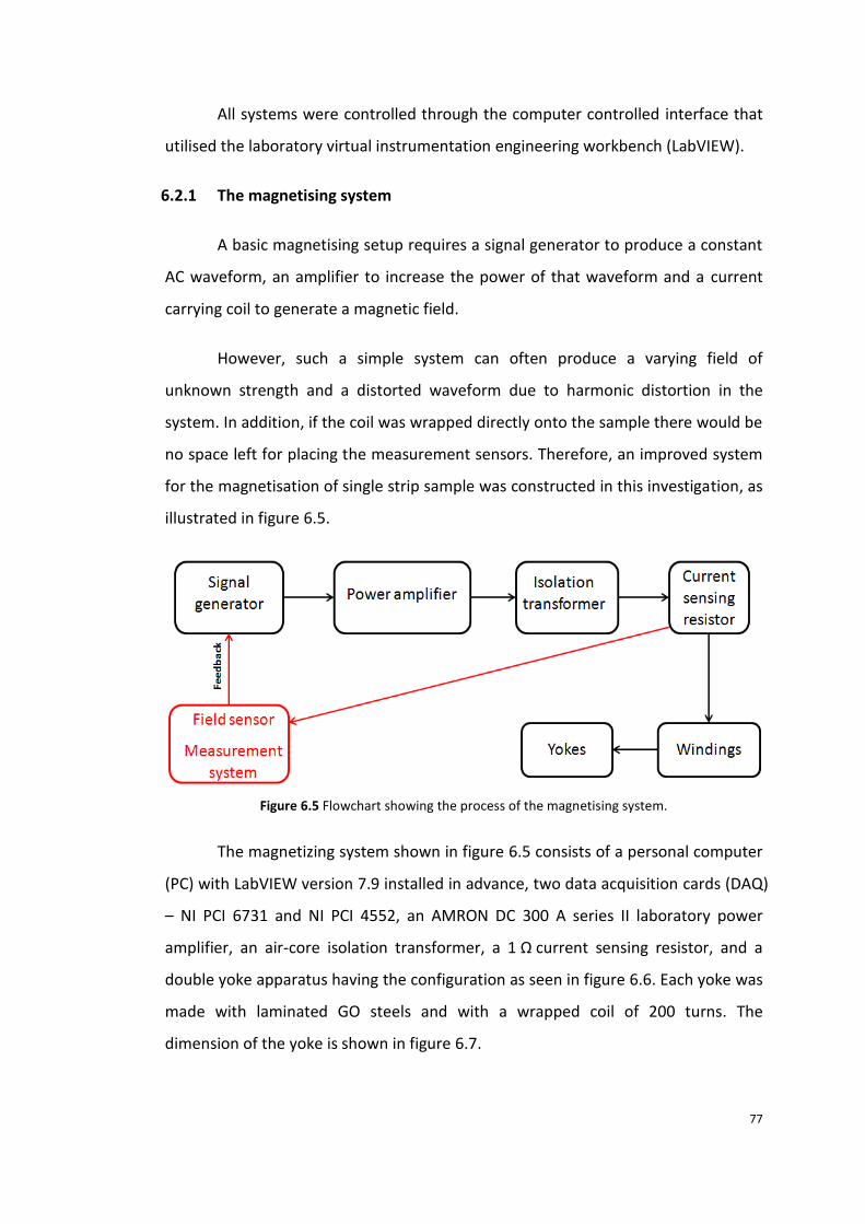
77

All systems were controlled through the computer controlled interface that

utilised the laboratory virtual instrumentation engineering workbench (LabVIEW).

6.2.1 The magnetising system

A basic magnetising setup requires a signal generator to produce a constant

AC waveform, an amplifier to increase the power of that waveform and a current

carrying coil to generate a magnetic field.

However, such a simple system can often produce a varying field of

unknown strength and a distorted waveform due to harmonic distortion in the

system. In addition, if the coil was wrapped directly onto the sample there would be

no space left for placing the measurement sensors. Therefore, an improved system

for the magnetisation of single strip sample was constructed in this investigation, as

illustrated in figure 6.5.

Figure 6.5 Flowchart showing the process of the magnetising system.

The magnetizing system shown in figure 6.5 consists of a personal computer

(PC) with LabVIEW version 7.9 installed in advance, two data acquisition cards (DAQ)

– NI PCI 6731 and NI PCI 4552, an AMRON DC 300 A series II laboratory power

amplifier, an air-core isolation transformer, a 1 Ω current sensing resistor, and a

double yoke apparatus having the configuration as seen in figure 6.6. Each yoke was

made with laminated GO steels and with a wrapped coil of 200 turns. The

dimension of the yoke is shown in figure 6.7.

78

Figure 6.6 Schematic diagram of the magnetizing apparatus.

Figure 6.7 Schematic diagram showing the dimension of the yoke.

The magnetizing waveform and voltage were produced by the PC/ LabVIEW

and NI PCI 6731 DAQ respectively, which were fed into the amplifier for the

required field strength. The output voltage was passed through an air-core isolation

transformer for the suppression of noise from the power supply. At this point, the

voltage across the resistor of a known resistance was measured by the NI PCI 4552

DAQ which was used to calculate the current passing through the coil and to derive

the field strength. The magnetizing field produced by the current carrying coil was

passed through the specimen via the double yokes, thus creating space to enable

79

local measurements to be conducted. Moreover, the use of the double yoke

configuration eliminates/cancels the in-plane eddy current formed at the poles of

the yokes (discussed in chapter 5).

However, the field or flux density applied to the specimen cannot be derived

by the field sensing resistor since the winding was not wrapped directly on the

specimen. To solve this problem the overall flux density of the specimen was

measured utilising a search coil that together constitutes the feedback (FB) system

with the field sensing resistor. The information of the field collected by the FB

system is used to compare it with the ideal field, and the differences will be

adjusted by the NI PCI 6731 DAQ so that the measurement can be carried out within

the set tolerance that was determined by the users via three main regulated control

criteria displayed on the front panel on the PC. The three control criteria were the %

error of peak flux density Bpeak value, the total harmonic distortion (THD) and the

form factor (FF) of the induced voltage in the search coil. The default values set for

the three control criteria were 0.1%, 1.5% and 0.5% respectively. These were also

upper limit values of the settings for all the measurements carried out throughout

the investigations.

6.2.2 The measurement system

The measurement system comprises the LabVIEW program, an NI PCI 4552

DAQ, an 80 turn search coil, four transducers, a local loss measurement sensor and

a Farnell stabilised DC power supply for operation of the local loss measurement

sensor.

The 80 turn search coil was made by wrapping closely a single layer of 0.1

mm diameter wire on a plastic matrix of 31 (L) x 6 (W) x 0.5 (T) mm. The coil was

placed next to the scanning area for measurement of the applied overall flux

density.

A local loss measurement sensor was designed and calibrated for the

measurement of the localised field H and flux density B, from which the power loss

at the measurement point was calculated (see equation 2.12 and 2.13 in chapter 2).

80

The measurement probe consists of a square printed circuit board (PCB) containing

two spring-loaded, 1.27 mm diameter phosphor bronze needles with an effective

separation of 7 mm and a Honeywell SS495A linear Hall Effect sensor with an

effective sensing span of 2 mm mounted between the needles, as illustrated in

figure 6.8 (a). In addition, an orthogonal needle probe, that made of the same type

of needles at the same 7 mm needle span as illustrated in figure 6.8 (b), was build

for the measurement of component of flux density in both rolling direction (RD) and

transverse direction (TD) in the test specimens in this investigation.

(a)

(b)

Figure 6.8 Illustration of the (a) localised loss measurement sensor and (b) orthogonal needle probe.

81

The design of making needles 7 mm apart is to provide the capability of

measurement of localised flux density within grains of HGO steel with reasonable

needle span to sample thickness ratio to meet the second assumption (see 5.1.2).

Calibration of the needle probe is detailed in the later chapter 8.3, where the

needle probe is compared with a single turn search coil for the measurement of

localised flux density on a HGO steel.

During the measurement, the distance between the sensing element in the

Hall Effect sensor and the sample surface was controlled by the positioning system

and was maintained at approximately 0.5 mm above the test sample. The spring

loaded needles were used to ensure continuous contact when the sample was

vibrating during magnetisation to avoid the loss of signals. The instantaneous flux

density B(t) was calculated from the instantaneous output voltage V(t) of the needle

probe by using the equation derived from 5.13, as shown below

𝐵(𝑡) =𝑉(𝑡)

2𝐴𝑓 (T)

The tangential component of instantaneous field H(t) along the

magnetisation direction was derived from the instantaneous output voltage V(t) of

the linear Hall Effect sensor operated at 5 V input DC current. The equation is

shown below

𝐻(𝑡) = 𝐶𝑉(𝑡) (A/m)

where C is the scaling factor of the Hall effect sensor.

The localised loss measurement sensor was placed securely in an aluminium

cantilever fixed on the positioning system, making it possible to scan the area of

interest. For example, to scan an area of 10 x 10 mm on the surface of a test

specimen with desired scanning resolution of 2 mm, as shown in figure 6.9. The

sensor is set to measure localised B and H of the 36 points in the number order. It

should be noted that each localised B measurement is an average of flux density in

between the 7 mm needle span, and each localised H measurement is an average of

82

magnetising field over the 2 mm area where the Hall sensor is located. The results

of measurements can be used to make contour map that showing the distribution

of localised B and H over this 10 x 10 mm scanning area.

Figure 6.9 Illustration of the process of scanning B and H measurements using the localised loss

sensor over a 10 x 10 mm surface area at 2 mm sampling intervals.

6.2.3 The positioning system

The positioning system consists of a PC/LabVIEW program, two interface

units (NI SCB-68 and NI CB68-LP), a Parker Daedal cross roller series positioner and

a self-made aluminium cantilever with a sensor holder at its free end shown in

figure 6.10. The positioning system was a completely separate system and only

communicated with the measurement system through a bridge created by the

interface units. Therefore, when scanning a specimen, the correct VIs (the ‘Scanning

local-loss’ VI for measurement and ‘Scanning position’ VI for positioning) must run

on both PCs simultaneously.

83

Figure 6.10 Dimension of the cantilever.

The Paker positioner is able to move in the three axes labelled X, Y and Z on

the stepper motors and the VI program was set to raster scan samples

automatically from left to right and top to bottom. The sampling rate or scanning

resolution can be set using the dx and dy controls on the VI’s front panel. The

starting position, point 0 as indicated in the scanning position VI, can be chosen by

the users through a separate VI program. Once the measurement is completed at

the first point, the cantilever/sensor is lifted by the Z motor, and then moved to the

next point and lowered to the same height so that the measurement can be

repeated; this process continues until the required number of moves has been

performed.

A dataflow diagram showing the measurement procedure is shown in figure

6.11. To start the test, the loss measurement VI reads the information regarding the

three criteria (% error of peak flux density value, THD and FF) for the overall flux

Side view

Bottom view

3D view

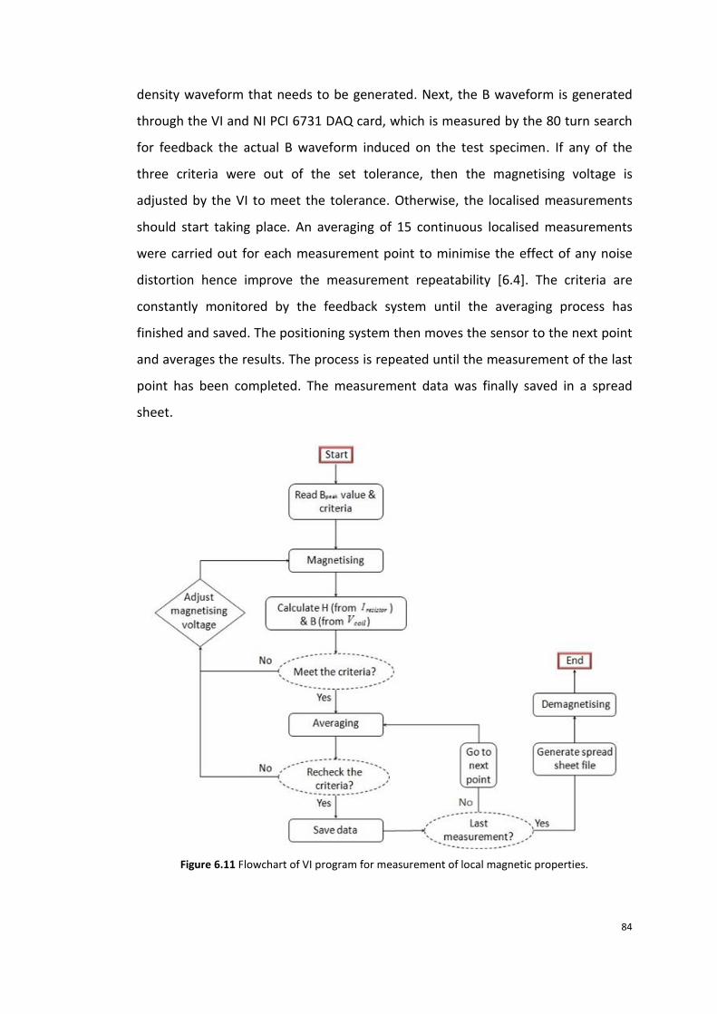
84

density waveform that needs to be generated. Next, the B waveform is generated

through the VI and NI PCI 6731 DAQ card, which is measured by the 80 turn search

for feedback the actual B waveform induced on the test specimen. If any of the

three criteria were out of the set tolerance, then the magnetising voltage is

adjusted by the VI to meet the tolerance. Otherwise, the localised measurements

should start taking place. An averaging of 15 continuous localised measurements

were carried out for each measurement point to minimise the effect of any noise

distortion hence improve the measurement repeatability [6.4]. The criteria are

constantly monitored by the feedback system until the averaging process has

finished and saved. The positioning system then moves the sensor to the next point

and averages the results. The process is repeated until the measurement of the last

point has been completed. The measurement data was finally saved in a spread

sheet.

Figure 6.11 Flowchart of VI program for measurement of local magnetic properties.

85

6.3 Uncertainty analysis

Measurement uncertainty is an evaluation of the interval of the result of the

measurement that describes how far the true value may differ from the result.

Analysis of the measurement uncertainty provides a level of confidence to a

measurement result.

In this investigation, all values of uncertainty were evaluated based on the

method stated in UKAS M3003 [6.5]. The sources of uncertainty need to be

converted into the same unit and at the same level of confidence before merging;

this was done by using the standard uncertainties 𝑢. There are two types of

evaluation for estimating the 𝑢 values: ‘type A’ and ‘type B’ evaluations. Type A is a

statistical method (e.g. from repeated measurements) whereas type B is a

systematic method (e.g. from past experience of the measurements, published

certificates, specifications provided by manufacturer and etc.).

In general, the estimated output quantity y, or the measurand, is affected by

a number (n) of influence quantities x by the mathematical relationship given as

y = f(x1, x2, … xn)

For type A evaluation, the standard uncertainty uA(y), is derived from

standard deviation s by the following equation

uA(y) =s

√n

where s is expressed as

s = √∑ (qi−q̅)2n

i=1

n−1

and qi is the measured value of 𝑦 and �̅� is the arithmetic mean of 𝑦. �̅� is expressed

as

(6.1)

(6.3)

(6.2)

86

�̅� =1

𝑛∑ 𝑞𝑖

𝑛𝑖=1

For type B evaluation, the components of uncertainty are represented by

the standard uncertainties of the measurement input 𝑥𝑖 and the output standard

uncertainty 𝑢𝐵(𝑦) is expressed as

𝑢𝐵2 (𝑦) = 𝑐1

2𝑢2(𝑥1) + 𝑐22𝑢2(𝑥2) + ⋯ + 𝑐𝑛

2𝑢2(𝑥𝑛)

where 𝑐𝑖 (𝑐1, 𝑐2, …,𝑐𝑛) is the sensitivity coefficient associated with each input 𝑥𝑖 and

is the partial derivative of the model function with respect to the input. Thus,

𝑐𝑖 =𝜕𝑦

𝜕𝑥𝑖

In the case of magnetic measurements the exact function relationship of the

measurement is unknown, i.e. 𝑐𝑖 cannot be derived mathematically so 𝑐𝑖 is

estimated by means of experimental method, from determination of ∂y/ ∂xi by

changing the value of 𝑥𝑖.

The uncertainty after summation in quadrature of individual standard

uncertainties as calculated by type A and type B evaluation is the combined

uncertainty 𝑢𝑐(𝑦), and is expressed as

𝑢𝑐(𝑦) = √𝑢𝐴2(𝑦) + 𝑢𝐵

2 (𝑦)

The combined uncertainty estimated from the above equation is considered

at confidence level of 68%. This uncertainty can be expanded at other levels of

confidence by multiplying the coverage factor 𝑘. Most commonly, the expended

uncertainty 𝑈 is given at confidence level of 95%, by the expression

𝑈(𝑦) = 𝑘95𝑢(𝑦)

(6.4)

(6.5)

(6.6)

(6.7)

(6.8)

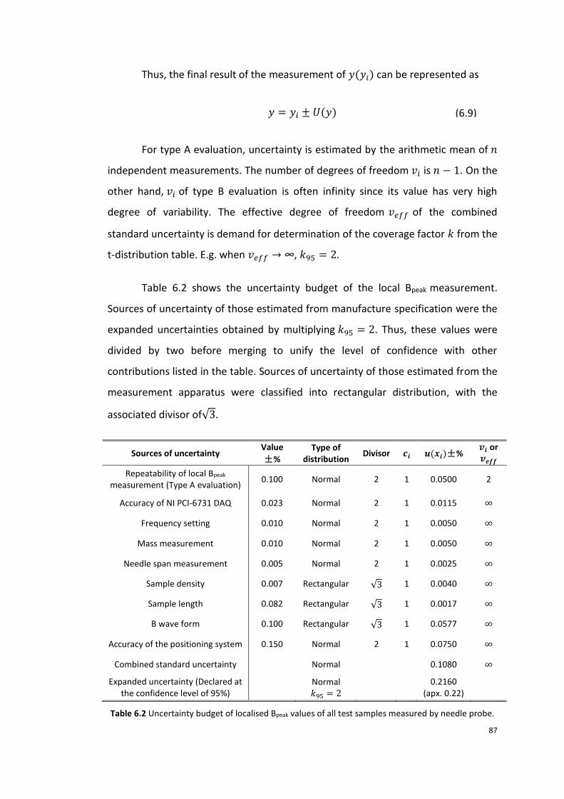
87

Thus, the final result of the measurement of 𝑦(𝑦𝑖) can be represented as

𝑦 = 𝑦𝑖 ± 𝑈(𝑦)

For type A evaluation, uncertainty is estimated by the arithmetic mean of 𝑛

independent measurements. The number of degrees of freedom 𝑣𝑖 is 𝑛 − 1. On the

other hand, 𝑣𝑖 of type B evaluation is often infinity since its value has very high

degree of variability. The effective degree of freedom 𝑣𝑒𝑓𝑓 of the combined

standard uncertainty is demand for determination of the coverage factor 𝑘 from the

t-distribution table. E.g. when 𝑣𝑒𝑓𝑓 → ∞, 𝑘95 = 2.

Table 6.2 shows the uncertainty budget of the local Bpeak measurement.

Sources of uncertainty of those estimated from manufacture specification were the

expanded uncertainties obtained by multiplying 𝑘95 = 2. Thus, these values were

divided by two before merging to unify the level of confidence with other

contributions listed in the table. Sources of uncertainty of those estimated from the

measurement apparatus were classified into rectangular distribution, with the

associated divisor of√3.

Sources of uncertainty Value

±% Type of

distribution Divisor 𝒄𝒊 𝒖(𝒙𝒊)±%

𝒗𝒊 or 𝒗𝒆𝒇𝒇

Repeatability of local Bpeak measurement (Type A evaluation)

0.100 Normal 2 1 0.0500 2

Accuracy of NI PCI-6731 DAQ 0.023 Normal 2 1 0.0115 ∞

Frequency setting 0.010 Normal 2 1 0.0050 ∞

Mass measurement 0.010 Normal 2 1 0.0050 ∞

Needle span measurement 0.005 Normal 2 1 0.0025 ∞

Sample density 0.007 Rectangular √3 1 0.0040 ∞

Sample length 0.082 Rectangular √3 1 0.0017 ∞

B wave form 0.100 Rectangular √3 1 0.0577 ∞

Accuracy of the positioning system 0.150 Normal 2 1 0.0750 ∞

Combined standard uncertainty Normal 0.1080 ∞

Expanded uncertainty (Declared at the confidence level of 95%)

Normal 𝑘95 = 2

0.2160

(apx. 0.22)

Table 6.2 Uncertainty budget of localised Bpeak values of all test samples measured by needle probe.

(6.9)

88

The basis of evaluation of sources of uncertainty in table 6.2 is detailed

below.

Repeatability of local Bpeak measurement. An experiment was conducted to

find the repeatability of localized B measurement at different level of

global applied B, 1.1 T, 1.5 T and 1.7 T. It was set by repeating

measurement three times at five selected points of each of the three test

samples of HiB steel. The highest repeatability was calculated by means of

using the highest difference between the values of the three

measurements taken at the same point divided by the smallest value of the

three measurements. As shown in table 6.3, the highest repeatability of all

measurements is given by ± 0.1%, this value is used for all evaluations in

the entire investigation.

Global B Meas 1 Meas 2 Meas 3 Repeatibility

1.1 T

Point 1 1.074 1.075 1.075 ±0.09%

Point 2 1.102 1.102 1.103 ±0.09%

Point 3 0.998 0.998 0.998 ±0.00%

Point 4 1.089 1.089 1.089 ±0.00%

Point 5 1.132 1.133 1.132 ±0.09%

1.5T

Point 1 1.617 1.616 1.616 ±0.06%

Point 2 1.695 1.695 1.695 ±0.00%

Point 3 1.305 1.304 1.305 ±0.08%

Point 4 1.491 1.491 1.491 ±0.00%

Point 5 1.553 1.553 1.552 ±0.07%

1.7T

Point 1 1.578 1.578 1.578 ±0.00%

Point 2 1.679 1.678 1.679 ±0.06%

Point 3 1.338 1.338 1.338 ±0.00%

Point 4 1.802 1.801 1.802 ±0.06%

Point 5 1.730 1.730 1.730 ±0.00%

Table 6.3 Repeatability of localised Bpeak measured using the needle probe.

Accuracy of NI PCI-6731 DAQ. The accuracy range of voltage output at

±10V is ±2.24mV according to the manufacture specifications. This gives

accuracy range in percentage is ±0.023%.

89

Frequency setting. ±0.01% variation is given by the base clock accuracy of

the DAQ.

Sample mass measurement. All samples were weight utilizing an Avery

Berkel balance with smallest division of 0.01 g. An average value of three

measurements was used for each sample, providing a calculated expanded

uncertainty of approximately ±0.01% for all samples.

Needle separation distance. The distance between two needle tips was

measured by moving sample stage with division of distance of 0.01 mm

under an optical microscope. The measurement was repeated five times

and produced a calculated expanded uncertainty of ±0.005% .

Sample density. The density of GO steel given by the manufacture is 7650

Kg/m3. Assuming the accuracy of the data is at ±0.5 Kg/m3, then the

relative accuracy in percentage is ±0.007.

Sample length. The assumed length of an Epstein sample is 305 mm. The

actual length of the test sample was measured utilizing a metal ruler with

division of 0.5 mm. Thus, the last digit of the reading can be estimated at

half of the division which provides an accuracy of ±0.25 mm, giving

relative accuracy of 0.082%.

B waveform control. Bpeak and form factor were set through LabVIEW

control at ±0.1% for all experiments conducted in the investigation.

Accuracy of the positioning system. The manufacture provided

specification of repeatability of ‘Parker cross roller series’ is ±3.0 μm. The

scanning resolution of all measurement is set to be 2 mm. Therefore, the

accuracy of the measurement utilising this positioning system is ±0.15%.

90

Sources of uncertainty Value

±% Type of

distribution Divisor 𝒄𝒊 𝒖(𝒙𝒊)±%

𝒗𝒊 or 𝒗𝒆𝒇𝒇

Repeatability of local Hpeak measurement (Type A evaluation)

0.2600 Normal 2 1 0.13000 2

Accuracy of NI PCI-6731 DAQ 0.023 Normal 2 1 0.0115 ∞

Frequency setting 0.010 Normal 2 1 0.0050 ∞

Accuracy of the positioning system 0.150 Normal 2 1 0.0750 ∞

Accuracy of the Hall effect sensor 1.040 Normal 2 1 0.5200 ∞

Accuracy of the input voltage 0.100 Normal 2 1 0.0500 ∞

Combined standard uncertainty Normal 0.5437 ∞

Expanded uncertainty (Declared at the confidence level of 95%)

Normal 𝑘95 = 2

1.0874

(apx. 1.09)

Table 6.4 Uncertainty budget of localised Hpeak values of all test samples measured by Hall Effect

sensor 50 Hz sinusoidal magnetisation.

The basis of evaluation of sources of uncertainty in table 6.4 is detailed below.

Repeatability of local Hpeak measurement. An experiment was conducted

to find the repeatability of localized Hpeak measurement at different

level of global applied B, 1.1 T, 1.5 T and 1.7 T. It was set by repeating

measurement three times at five selected points of each of the three

test samples of HiB steel. The uncertainty of repeatability at the worst

point is ± 0.26%. This value is therefore suitable for all cases evaluation.

Accuracy of the Hall Effect sensor. When operated at 𝑉𝑠𝑢𝑝𝑝𝑙𝑦 = 5 V, the

typical linearity span of ‘Honeywell’ SS495A1 Hall sensor given by

manufacture specification is ±1% and typical temperature error null

drift is ±0.04%. Thus, the estimated accuracy of the Hall Effect sensor is

the summation of the two values.

Accuracy of the power supply. An operating voltage of 5 V was applied

to the Hall Effect sensor utilising a Farnell stabilised power supply. The

output value was checked against a Mastech MY-67 multi-meter with

accuracy of ±0.1 % given by manufacture.

91

Sources of uncertainty Value

±% Type of

distribution Divisor 𝒄𝒊

𝒖(𝒙𝒊)±%

𝒗𝒊 or

𝒗𝒆𝒇𝒇

Repeatability of local P measurement (Type A evaluation)

0.82 Normal 2 1.5 0.62 2

H measurement 1.09 Normal 2 1 0.60 ∞

B measurement 0.22 Normal 2 1 0.15 ∞

Combined standard uncertainty Normal 0.88 ∞

Expanded uncertainty (Declared at the confidence level of 95%)

Normal 𝑘95 = 2

1.76

Table 6.5 Uncertainty budget of localised P values of all test samples measured by Hall effect sensor

50 Hz sinusoidal magnetisation.

The uncertainty of repeatability at the worst point of all measurements was

± 0.82%. This value was used for all cases of evaluation. Ci of localised P

measurement of 1.5 was obtained by reviewing the relationship between B and P

over the studied B field range (1.0 to 1.7 T) in this investigation. The ratio of dB/dP

increases as increasing overall applied flux density as shown in figure 6.12. The

highest ratio was approximately equal to 1.5 and was used in this investigation.

Figure 6.12 Relationship between power loss of HGO steel and overall applied flux density measured using a single strip tester.

0.00E+00

2.00E-01

4.00E-01

6.00E-01

8.00E-01

1.00E+00

1.20E+00

1.40E+00

1.60E+00

1.80E+00

1.00E-01 4.00E-01 6.99E-01 1.00E+00 1.30E+00 1.60E+00 1.90E+00

Po

we

r lo

ss (

W/K

g)

Bpeak (T)

92

Sources of uncertainty Value

±% Type of

distribution Divisor 𝒄𝒊 𝒖(𝒙𝒊)±%

𝒗𝒊 or 𝒗𝒆𝒇𝒇

Repeatability of local Bpeak measurement (Type A evaluation)

0.100 Normal 2 1 0.0500 2

Accuracy of NI PCI-6731 DAQ 0.023 Normal 2 1 0.0115 ∞

Frequency setting 0.010 Normal 2 1 0.0050 ∞

Mass measurement 0.010 Normal 2 1 0.0050 ∞

Cross sectional area measurement 0.010 Normal 2 1 0.0050 ∞

Sample density 0.007 Rectangular √3 1 0.0040 ∞

Sample length 0.082 Rectangular √3 1 0.0017 ∞

B wave form 0.100 Rectangular √3 1 0.0577 ∞

Combined standard uncertainty Normal 0.0782 ∞

Expanded uncertainty (Declared at the confidence level of 95%)

Normal 𝑘95 = 2

0.1563

(apx. 0.16)

Table 6.6 Uncertainty budget of localised Bpeak values measured using search coil.

93

References

[6.1] X. Xu, A. Moses, J. Hall, P. William and K. Jenkins, “A comparison of magnetic domain images using a modified Bitter pattern technique and the Kerr method on grain-oriented electrical steel”, IEEE Transactions on Magnetics, vol. 47, pp. 3531 – 3534, (2011).

[6.2] Available online at www.downloads.techimaging.com/docs/Fastcam_MC1_HW_Manual_Rev100en.pdf, last accessed on 3rd Nov. 2013.

[6.3] O. Hoshtanar, “Dynamic domain observation in grain-oriented electrical steel using magneto-optical techniques”, PHD Thesis, Cardiff University, (2006).

[6.4] S. Zurek, P. Marketos, P. I. Anderson, and A. J. Moses, "Influence of digital resolution of measuring equipment on the accuracy of power loss measured in Epstein frame," Przegląd Elektrotechniczny (Electrical Reviews), Vol. R. 83, pp. 50-53, (2007).

[6.5] UKAS M3003, ‘The expression of uncertainty and confidence in measurement’, 2nd edition, (2007).

94

Chapter 7

Specimen Selection and Preparation

7.1 Selection of test specimens

Epstein specimens of 305 mm x 30 mm for the study of local magnetic

properties were cut from a square sheet of 500 x 500 mm using a mechanical

guillotine. All test material was provided by Cogent Power Ltd. in Newport, UK, and

it is a type of commercial HiB steel with manufactures specifications are shown in

table 7.1. The polarisation at H = 800 A/m (or BH=800) shown in table 7.1 is often

used by electrical steel manufactures to describe magnetic property of their

products. Material with higher value of BH=800 usually shows lower measured power

loss.

Product

code

Thickness

(mm)

Maximum specific loss

(W/Kg) at 1.7 T, 50 Hz

Typical specific loss

(W/Kg) at 1.7 T, 50

Hz

Polarisation (T) at

H = 800 A/m (50

Hz)

M111-30P 0.30 1.11 1.08 1.93

Table 7.1 Typical specifications provided by the manufacture. [7.1]

Apart from the commercial specimens listed above, additional Epstein size

0.3 mm thick, poorly oriented electrical steel was prepared in the laboratory to

have an extremely poor texture. It was use in this investigation for the study of the

effect of grain misorientation on the variation of local magnetic properties.

95

Table 7.2 shows the specifications of all Epstein specimens studied in this

investigation, including seven commercial HiB specimens (coded H1 – H7) and one

poorly oriented specimen (P1). Assuming specimens contain round grains, the

average grain diameter D in table 7.2 is calculated from equation below

D = 2 × √A

Nπ

where A is the surface area of the Epstein specimen (305 mm x 30 mm) and N is

number of grains in the specimen assessed using both visual inspection and Orb

domain viewer inspection.

The yaw angle, which is the in-plane deviation angle of the grain orientation

[001] from the RD of the specimen, was measured by assessing the deviation angles

of bar domains observed using the domain viewer. The specimens were decoated

and stress relief annealed prior for all experiments carried out in this investigation

(annealing procedure is outlined in 7.2). The power loss values shown in table 7.2

were measured thereafter using a single strip tester which is calibrated with respect

to a standard Epstein square. Relatively higher power loss values are shown in table

7.2 in comparison with the manufacture specification, which is due to removal of

the insulation coatings that provide beneficial effect on the overall power loss of

the steel. It can be considered that the thickness of coatings is uniform so removal

of the coatings will have no significant effect on the distribution of localised

magnetic properties.

Specimen Average grain

diameter D (mm) Average yaw angle

deviated from RD (°) Power loss1.7T/50Hz

(W/Kg) BH=800 (T)

H1 10.0 3 1.23 1.92

H2 10.8 3 1.25 1.90

H3 10.3 3 1.27 1.88

H4 9.8 3 1.25 1.90

H5 10.4 3 1.26 1.90

H6 10.1 3 1.20 1.92

H7 9.9 3 1.25 1.90

P1 12.3 18 2.40 1.55

Table 7.2 Specifications of the Epstein specimens.

96

7.2 Preparation of test specimens

7.2.1 Preparation of Epstein strips for local loss measurement.

Coating removal – To ensure needle signal quality, the insulation coating of

all test specimen was removed in a HCL bath of 38% concentration. During the

process of chemical reaction, constant inspection was involved to avoid over-

etching of the test specimen. Once the coating layer was removed, the specimen

was soaked in an Acetone bath of 99% concentration to wash away the remaining

acid. After which specimen was rinsed with Kemet cleaning fluid CO42 and dried up

using clean paper towel to prevent it from further oxidation.

Stress relief annealing – Annealing is required to remove stresses that are

added in the steel during material handling. The process was carried out after the

coating had been removed on both surfaces of specimen. A PC-controlled Elite

vacuum tube furnace with a set programme shown in table 7.3 was used for stress

relief anneal of all test specimens. To prevent specimen oxidation, a minimum

pressure of less than 10-5 mbar was maintained using the build-in turbo pump

throughout the entire annealing process.

Segment Program Temperature (oC) Heating Rate (oC /

hour)

1 Heating up Room temperature – 810 250

2 Duration 810 oC for 1 hour 0

3 Cooling down 810 oC – room temperature -50

Table 7.3 Annealing programme for stress relief annealing of electrical steel specimens.

7.2.2 Preparation of specimens for Kerr microscope observation.

Specimens for Kerr microscope observation were metallurgical prepared to a

mirror surface finishing. The procedure consists of grinding and polishing which was

carried out using the Struers magnetic disc (MD) machine. The specifications of the

corresponding grinding and polishing discs used in the metallurgical preparation are

97

listed in table 7.4, in which discs 1 & 2 are grinding discs and discs 3 & 4 are

polishing discs.

No. Disc code Disc diameter

(mm) Roughness (µm) Abrasive fluid

1 MD-Piano 600 300 15.3 Water

2 MD-Largo 300 9 Water + Largo diamond

suspension

3 MD-Dac 300 9-3 DP-Lubricant + Dac diamond

suspension

4 MD-Nap 300 ≤1 DP-lubricant + Nap diamond

suspension

Table 7.4 Specifications of the grinding and polishing discs for preparation of the specimens

for Kerr microscope examination.

Sharp corners and edges of the specimens were removed using a silicon

carbide paper prior the metallurgical preparation as to protect the preparation discs

from scratches. For an easy grip, specimens to be prepared were pasted onto pre-

made sample holders using high strength, double sided tape.

Specimens after metallurgical preparation were heated up in a laboratory

furnace at 130 oC to soften the tape so that the specimens could be separated from

their holders. Specimens thereafter were stress relief annealed using the method

outlined in 7.1 for the removal of residual stresses which were added by the

mechanical grinding process.

98

Reference

[7.1] http://www.cogent-power.com/unisil-h/unisil-h-guaranteed-magnetic-properties/, last

accessed on 8th Feb 2014.

99

Chapter 8

Results and Discussion

8.1 Introduction

Domain observation is frequently involved throughout the entire

investigation in the study of magnetic characteristic of test specimens presented in

this chapter. Static domain patterns were observed for assessing the grain

orientation of test specimens and the domain wall spacing of the domain scribed

specimen. Dynamic domain observations were carried out in the study of domain

wall movement; and to help improve the understanding of localised non-uniform

magnetisation in grain oriented electrical steels.

The domain viewer and magneto-optical Kerr microscope were used for

observing domain structures. A comparative study was carried out as described in

8.2 to explain differences in the domain pattern on the same specimen under the

same conditions observed using these techniques.

The needle probe for measurement of localised flux density is outlined in

chapter 6. A test to assess the accuracy of the needle probe on measurement of

localised flux density is described in 8.4.

Components of localised flux density in rolling and transverse directions of a

HiB specimen, measured using an orthogonal needle probe, are presented in 8.5.

100

The transverse flux density is compared with rolling flux density so that the effect of

transverse flux density on power loss of HiB steel could be quantified.

Localised flux density at different levels of magnetic induction was measured

using the needle probe on a HiB specimen and is presented in 8.6 and the influence

of induction level on the degree of variation of flux density is discussed.

Localised flux density, magnetic field and power loss was measured in the

commercial HiB specimen and the laboratory produced poorly oriented specimen

using the local loss measurement system outlined in chapter 6. The results are

displayed in 8.8 and the effect of grain misorientation on the distribution of

localised magnetic properties is discussed.

Localised magnetic flux density of specimen H7 before and after scribing

were measured using the local loss measurement system and is presented in 8.9

and the influence of domain refinement on the distribution of localised magnetic

flux density could be analysed.

101

8.2 Differences in observed magnetic domain structures found using

domain viewer and magneto-optical Kerr techniques

Differences between magnetic domain patterns on the surface of specimen

H1 were obtained using the domain viewer and the magneto-optical Kerr

microscope. Both techniques are widely used for observation of magnetic domain

pattern on electrical steels but such differences have not been reported previously.

The sample whose surface was observed was a 25 mm square HiB steel cut

from H1. The sample was decoated, metallurgical prepared as described in chapter

7 and stress relief annealed prior the domain observation. The grain boundary was

not found through optical observation after the sample was chemically etched. An

EBSD analysis was carried out at Tata Steel Swinden Technology Centre, UK to study

the crystallographic texture of the test sample and to prove the existence of the

grain boundary.

Surface domain structure of the prepared sample was observed using the

domain viewer and Kerr microscope respectively. Due to the observation limitation

of the Kerr microscope, the Kerr observation was carried out by means of scanning

sample surface under the microscope.

Figure 8.1 shows the typical anti-parallel bar domain patterns obtained using

the domain viewer and the Kerr microscope on the demagnetised sample. The

Bitter domain pattern shows a discontinuity in the domain contrast typical of the

effect of grain boundary oriented transverse to the RD of the specimen. The Kerr

image shows continuous domain magnetisation over the 8 mm x 6 mm area where

the possible effect of a grain boundary was found in the Bitter image. No evidence

of a grain boundary in the surrounding surface was found using the Kerr microscope.

The same number of domains (17 black domains and 17 white domains) was

observed using both techniques.

102

Figure 8.1 (a) Bitter domain image of the whole surface of the 25 x 25 mm specimen observed using

the domain viewer, (b) the corresponding Kerr image in the area located inside the dash box [8.1].

In order to confirm that the vertical magnetic field applied in the domain

viewer was not the cause of the different images, a vertical DC field of the same

strength (approximately 2.2 KAm-1) as used in the domain viewer was applied to the

test specimen using a current conducting coil during the Kerr microscope

observation. No change of domain contrast was observed.

Figure 8.2 shows the crystallographic texture of the sample obtained from

EBSD analysis on the same area as presented in the 8 mm x 6 mm area covered by

Kerr image shown in figure 8.1b. The colour-coded map reveals a grain boundary

indicated by the lighter and darker yellow boundary, which consistent with that

seen in the dash box in figure 8.1a. The misorientation profile shows that the

relative misorientation angle between two crystals were less than 1o.

103

(a)

(b)

Figure 8.2 (a) EBSD colour-coded map shows crystal orientation of the area included in the

Kerr image of figure 8.1b, (b) misorientation profile scanned along the transverse direction in (a)

[8.1].

In this case, two observation techniques have clearly presented inconsistent

information regarding grain boundary and domain magnetisation. However, the

number of domains and domain alignment were observed the same using both

techniques.

A simple model showing crystal orientation and domain magnetisation of

the adjacent grains is illustrated in figure 8.3. As shown in figure 8.3a, the easy

magnetising axes [001] indicated by the cubes are slightly deviated with respect to

104

the surface plane and with respect to each other, as a result, leading to a leakage

field on the surface of the specimen shown in figure 8.3b. When an external DC field

is applied perpendicular to the surface plane, magnetic dipoles indicated by arrows

in figure 8.3b are rotating toward the direction of the field. Therefore, leading to

dipoles in one type of domains to coherently rotate towards the surface plane and

dipoles in the other type domain to coherently away from the surface plane, since

the contrast from the domain viewer is based on the strength of the surface leakage

field. As a result, a reversal in domain contrast is developed in the domain viewer.

No reversal in Kerr image contrast was observed, since the Kerr effect senses the

magnetisation parallel to the surface of the specimen and the overall magnetisation

continuous across the grain boundary with and without the presence of the vertical

DC field.

Figure 8.3 Cross sectional view of the test specimen with crystallographic cubes indicating the crystal

orientation and arrows indicating the orientation of magnetic dipoles.

105

8.3 Domain wall movement at grain boundary in sample of grain

oriented electrical steels.

An observation of domain wall movement at the small angle grain boundary

was carried out using the real time dynamic Kerr microscope system to study the

behaviour of dynamic domain on the surface of the sample whose static domain

pattern and crystallographic texture was studied in 8.2.

Domains in mismatched grains are often difficult to be clearly presented

simultaneously under the Kerr microscope, because the quality of Kerr image

depends on how well the plane of incident/reflection light is aligned with the

direction of domain magnetisation. Thus, the sample containing small angle grain

boundary was selected in this study.

Dynamic domain study was carried out using the dynamic Kerr microscope

outlined in chapter 6 at 50 Hz triangular flux density magnetisation. The use of

triangular magnetisation was to apply an overall constant dB/dt in the sample for

the study of uniformity of localised domain wall motion. The peak flux density at

surface domain saturation, measured using single turn search coil wound across the

entire cross section of the sample, was 1.20 T. It should be mentioned that eddy

current led to domain wall bowing will cause domain wall move faster at the surface

than in the middle, thus surface domain saturation occurs at lower flux density

compared to the overall saturation flux density (∼2.1 T) of the specimen.

Domain wall motion over the 6 mm x 6 mm area at the grain boundary was

captured using the high speed camera at a recording speed of 2000 frames per

second and resolution of 512 x 512 pixels (equivalent to 40 frames per magnetising

cycle). Prior presenting the dynamic images, it should be mentioned here that

dynamic domain pattern can be significantly different from static domain pattern

due to domain reconfiguration at power frequency.

The video clip was processed through the LabVIEW vision assistant 7.1 video

analysis software for contrast enhancement. This software allows the video to be

saved into groups of individual images which were then edited with analysis tools

106

provided in the software. In this experiment, background subtraction and contrast

improvement functions were used for improving the image contrast.

Domain pattern captured over 6 mm x 6 mm area at one instant time at 50

Hz magnetisation using the high speed camera is shown in figure 8.4. The black and

white strips represent the anti-parallel bar domains whose magnetisation direction

is indicated by the red arrows. At this instant time, surface domain saturation

occurred in the left grain thus uniform contrast is seen. Grain boundary is identified

by the disjointed bar domains and is indicated by the red line. The enlarged image

shows that the grain boundary is not a straight line but is in zigzag shape.

Figure 8.4 Image captured at 50 Hz magnetisation over 6 mm x 6 mm area where grain boundary is

found using domain viewer.

107

Figure 8.5 shows a sequence of domain images captured at time interval of

0.001 second in one complete magnetising cycle at 50 Hz triangular magnetisation.

Their corresponding moment of image capture is shown on the triangular waveform

below. The direction of domain magnetisation is indicated by the red arrows.

Figure 8.5 Kerr images showing the process of domain wall movement at 50 Hz triangular

magnetisation and 1.20 T peak flux density, and area of view is 6 mm x 6 mm at the location where

the small angle grain boundary is found in the 25 mm square sample studied in 8.2.

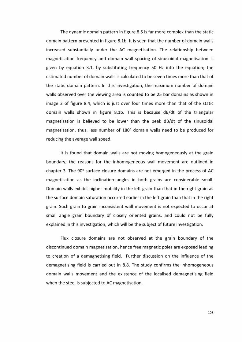
108

The dynamic domain pattern in figure 8.5 is far more complex than the static

domain pattern presented in figure 8.1b. It is seen that the number of domain walls

increased substantially under the AC magnetisation. The relationship between

magnetisation frequency and domain wall spacing of sinusoidal magnetisation is

given by equation 3.1, by substituting frequency 50 Hz into the equation; the

estimated number of domain walls is calculated to be seven times more than that of

the static domain pattern. In this investigation, the maximum number of domain

walls observed over the viewing area is counted to be 25 bar domains as shown in

image 3 of figure 8.4, which is just over four times more than that of the static

domain walls shown in figure 8.1b. This is because dB/dt of the triangular

magnetisation is believed to be lower than the peak dB/dt of the sinusoidal

magnetisation, thus, less number of 180o domain walls need to be produced for

reducing the average wall speed.

It is found that domain walls are not moving homogeneously at the grain

boundary; the reasons for the inhomogeneous wall movement are outlined in

chapter 3. The 90o surface closure domains are not emerged in the process of AC

magnetisation as the inclination angles in both grains are considerable small.

Domain walls exhibit higher mobility in the left grain than that in the right grain as

the surface domain saturation occurred earlier in the left grain than that in the right

grain. Such grain to grain inconsistent wall movement is not expected to occur at

small angle grain boundary of closely oriented grains, and could not be fully

explained in this investigation, which will be the subject of future investigation.

Flux closure domains are not observed at the grain boundary of the

discontinued domain magnetisation, hence free magnetic poles are exposed leading

to creation of a demagnetising field. Further discussion on the influence of the

demagnetising field is carried out in 8.8. The study confirms the inhomogeneous

domain walls movement and the existence of the localised demagnetising field

when the steel is subjected to AC magnetisation.

109

8.4 Evaluation of needle probe analysis of flux density in HiB

electrical steel.

Previous studies outlined in chapter 5 showed that the accuracy of the

needle probe technique can be affected by the inhomogeneous nature of the test

material. For grain oriented electrical steels, flux density measurement obtained

using needle probe and search coil can be differ by more than 10 % [8.2]. Therefore,

experiments were set up to test the accuracy of the bespoke needle probe for

measurement of localised flux density in commercial HiB specimens.

8.4.1 Comparison of flux density measurement using the needle probe on

opposite surfaces of a HiB specimen.

In needle probe measurement, it is assumed that the flux density is

symmetrically distributed with respect to the centre line of the cross sectional area

of the test specimen so that needle measurement need only be conducted on one

side of specimen. However, the flux density may not be consistent through the

thickness of grain oriented steel due to the material is considered to have higher

level of inhomogeneity compared with non-oriented electrical steel. Therefore,

needle probe measurements obtained from opposite surfaces of a HiB specimen

were compared.

Specimen H2 was selected, decoated and annealed prior to measurement.

The specimen was magnetised using the local loss measurement system outlined in

chapter 6 at sinusoidal flux density at 50 Hz and peak flux density of 1.50 T. The

localised peak flux densities in a 64 mm rolling direction (RD) x 20 mm transverse

direction (TD) area in the centre of the Epstein strip shown in figure 8.6 were raster

scanned using the needle probe at 2 mm sampling intervals. This corresponds to a

total sampling point of 363 in the scanning area. After the measurements were

completed, the specimen was turned upside down and the experiment was

repeated over an identical area of the other surface of the specimen.

110

Figure 8.6 Photograph of the scanning area of the H2 strip.

Figure 8.7 shows distribution of localised peak RD component of flux density

measured on opposite surfaces of H2 at sinusoidal magnetisation of 50 Hz and

overall applied peak flux density of 1.50 T. It can be seen that distribution patterns

obtained on both surfaces of the specimen are similar. At over peak flux density of

1.50 T, the average of flux density measurements derived from 363 localised

measurements is 1.52 T and 1.51 T on two surfaces respectively shown in table 8.1,

which corresponding to a difference of 0.7 % and 1.3 %.

Figure 8.8 shows percentage difference between needle measurements

obtained on opposite surfaces of the test specimen, derived from,

% difference = Btop − Bbottom

Btop× 100

Btop is localised peak flux density value from needle probe measurement obtained

on top surface of the specimen and Bbottom is the corresponding localised peak flux

density value from needle probe measurement obtained on bottom surface of the

specimen. The percentage difference between needle probe measurements

obtained on opposite surfaces varies across the scanning area from -13 % to 10 %.

Most regions show small differences, the average difference derived from 363

sampling point is 1.9 % shown in table 8.1. Regions showing higher differences are

randomly distributed, there is no correlation found between distribution of

differences and grain boundary pattern. The result presented here indicates that

flux density induced in two sides of the commercial HiB specimen may vary slightly.

111

Thus, to improve the accuracy of NP method on measurement of flux density, it is

recommended to use the average flux density measured in opposite sides of the

grain oriented steel.

Figure 8.7 Distribution of localised peak RD component of flux density obtained using the needle

probe on opposite surfaces of a commercial specimen.

Figure 8.8 Percentage differences between localised peak flux density values obtained on opposite

surfaces of a commercial HiB specimen, and grain boundary outlines are superimposed on the

contour map.

(mm)

(mm)

(T) (mm)

(mm) (T)

112

Average of localised peak flux

density Average of difference between top and bottom measurements

Top surface 1.52 T 1.9 %

Bottom surface 1.51 T

Table 8.1 Average localised flux density and percentage difference between needle measurements

obtained on top and bottom surfaces of the HiB specimen.

8.4.2 Comparison of localised flux density measurement using the needle probe

and search coil methods.

In this part of the experiment, a direct comparison of flux density

measurement using the needle probe and single turn search coils was carried out

on localised regions of a HiB specimen.

Specimen H3 was decoated and annealed prior to the measurement. Six

areas in the central section of the Epstein strip shown in figure 8.9 were selected.

The areas are evenly distributed across the diagonal of the central section; each

measurement position is separated by 10 mm (in the RD) and 3 mm (in the TD) from

its nearby position(s). The black dots indicate the point where needles and search

coil holes were located.

Figure 8.9 Positions of the localised needle probe and search coil measurements on the H3 strip.

The specimen was magnetised using the local loss measurement system at

sinusoidal flux density at 50 Hz and peak flux density of 1.50 T. Localised flux density

measurements at the six positions marked in figure 8.9 were made using the NP on

113

one surface of the specimen. The specimen was then turned over and the

measurements were repeated over the corresponding areas on the other surface.

Next, 0.5 mm diameter holes were drilled at each needle contact point. Single turn

search coils of 0.2 mm diameter enamelled copper wire were wound through each

pair of holes so that the localised flux density could be measured at each of the

needle probe measurement positions. It should be noted that the effective distance

enclosed by the SC is the same as that of the NP as described in chapter 5. Finally,

the search coil wires were removed and the specimen was stress relief annealed to

remove the residual stresses caused by drilling, new search coil wires were wound

thereafter at each position and the same measurements were repeated.

Localised flux density measurements obtained using needle probe and

search coil method respectively at the six local areas on the HiB specimen at 50 Hz

and peak flux density of 1.50 T are compared in table 8.2. The percentage

differences in measurements before and after anneal was calculated from,

% difference in SC measurements = Bafter anneal − Bbefore anneal

Bafter anneal× 100

The percentage differences in NP and SC measurements was calculated as,

% difference in NP and SC = BNP − BSC after anneal

BNP× 100

Position Measurements obtained using

NP

Measurements obtained using SC % difference between NP and SC after

anneal Before anneal

After anneal

% difference

1 1.48 T 1.38 T 1.52 T 9.2 -2.7

2 1.53 T 1.36 T 1.54 T 11.7 -0.7

3 1.59 T 1.65 T 1.61 T -2.5 -1.3

4 1.37 T 1.53 T 1.38 T -10.9 -0.7

5 1.30 T 1.42 T 1.29 T -10.1 0.8

6 1.55 T 1.71 T 1.53 T -11.8 1.3

Table 8.2 Comparison of localised flux density measurement obtained using the NP and SC methods

on the HiB specimen at 50 Hz and peak flux density of 1.50 T.

114

The result shows that the stress caused by drilling holes has a substantial

influence on localised flux density measurement using the SC when 0.5 diameter

holes were drilled at 7 mm span. Annealing removes elastic residual stress

introduced by drilling process, but cannot fully restore domain structure as the new

flux closure domains are formed and the remaining plastic stress may continue to

cause distortion on flux path. Therefore, the technique is still considered as a

destructive method for measurement of localised flux density. In this study, holes of

0.5 mm diameter were drilled for minimising the effect of drilling on accuracy of SC

measurement since the smallest drill available was 0.5 mm.

The percentage difference between flux density measured using NP and

those measured after annealing using SC varies between -2.7 % to 1.3 %. It is note

that the measurement uncertainties for both methods are estimated small, ±0.22 %

for NP and ±0.16 % for SC. Thus, the effect of uncertainty on the comparison is

neglected.

The results here show that through averaging flux densities derived from

opposite surfaces in NP measurement and stress relief anneal the specimen after

drilling holes in SC measurement, the two methods are able to provide consistent

measurements on grain oriented electrical steel.

115

8.5 2-D measurement of local magnetic flux density using the

orthogonal needle probe.

The components of flux density in both RD and TD in commercial HiB steel

were measured using the orthogonal needle probe and were compared with each

other to study the influence of the TD component of flux density on distribution of

localised flux density.

Specimen H4 was decoated and annealed prior to the experiment. The

specimen was magnetised using the local loss measurement system at sinusoidal

flux density magnetisation of 50 Hz and peak flux density of 1.50 T. An area of 64

mm (RD) x 20 mm (TD) in the centre of the strip shown in figure 8.10 was raster

scanned using the ONP at 2 mm sampling intervals. The measurement was repeated

on the identical area of both surfaces and average was plotted as contour

distribution maps.

Figure 8.11 shows the distribution of the components of localised flux

density measured using the ONP in the rolling and transverse directions and the

resultant. The resultant flux density Bresultant was calculated from the components

using the equation below,

Bresultant = √Brolling2 + Btransverse

2

where Brolling is the RD component of flux density and Btransverse is the TD component

of flux density.

116

Figure 8.10 Bitter domain pattern obtained using the domain viewer over the centre section of the

H4 strip.

(a)

(b)

(c)

Figure 8.11 Distribution of localised flux density at sinusoidal magnetisation of 50 Hz and overall

peak flux density of 1.50 T over the same region of specimen H4 shown in the box in figure 8.10. (a)

RD component of flux density, (b) TD component of flux density and (c) resultant flux density.

(mm)

(T)

(T)

(mm)

(mm)

(mm)

(mm)

(mm)

(T)

117

Table 8.3 shows average localised flux density measurements derived from

363 localised measurements for components of flux density measured in RD and TD

and the resultant flux density.

Average RD component of flux density

Average of TD component of flux density

Average resultant flux density

1.51 T 0.13 T 1.52 T

Table 8.3 Average localised flux density.

At overall peak flux density of 1.50 T, RD component of localised flux density

is found to vary in a range from 1.18 to 1.82 T, TD component of localised flux

density is found to vary in a range from 0.05 to 0.25 T. The average of components

of localised flux density measured in RD and TD is 1.51 T and 0.13 T respectively

shown in table 8.3, the TD component of localised flux density is found equivalent

to 8.6 % of the RD component of localised flux density.

Figure 8.11a and 8.11c show distributions of RD component of localised flux

density and the resultant localised flux density respectively. Very similar trends in

flux distributions are seen between these two distribution maps. The average

localised resultant flux density increased by less than 0.01 T or 0.6 % compare to

that of measured in RD alone. The result shows that the TD component of flux

density is relatively small and distributed more uniformly compared to that of the

RD component. For the study of distribution of localised flux density in HiB steel, it

is not necessary to take into account of the TD component of flux density.

Further study on TD component of flux density is presented in 8.7, where the

TD component of flux density in a poorly oriented specimen is compared with a HiB

specimen to study the correlation between grain misorientation on TD component

of flux density.

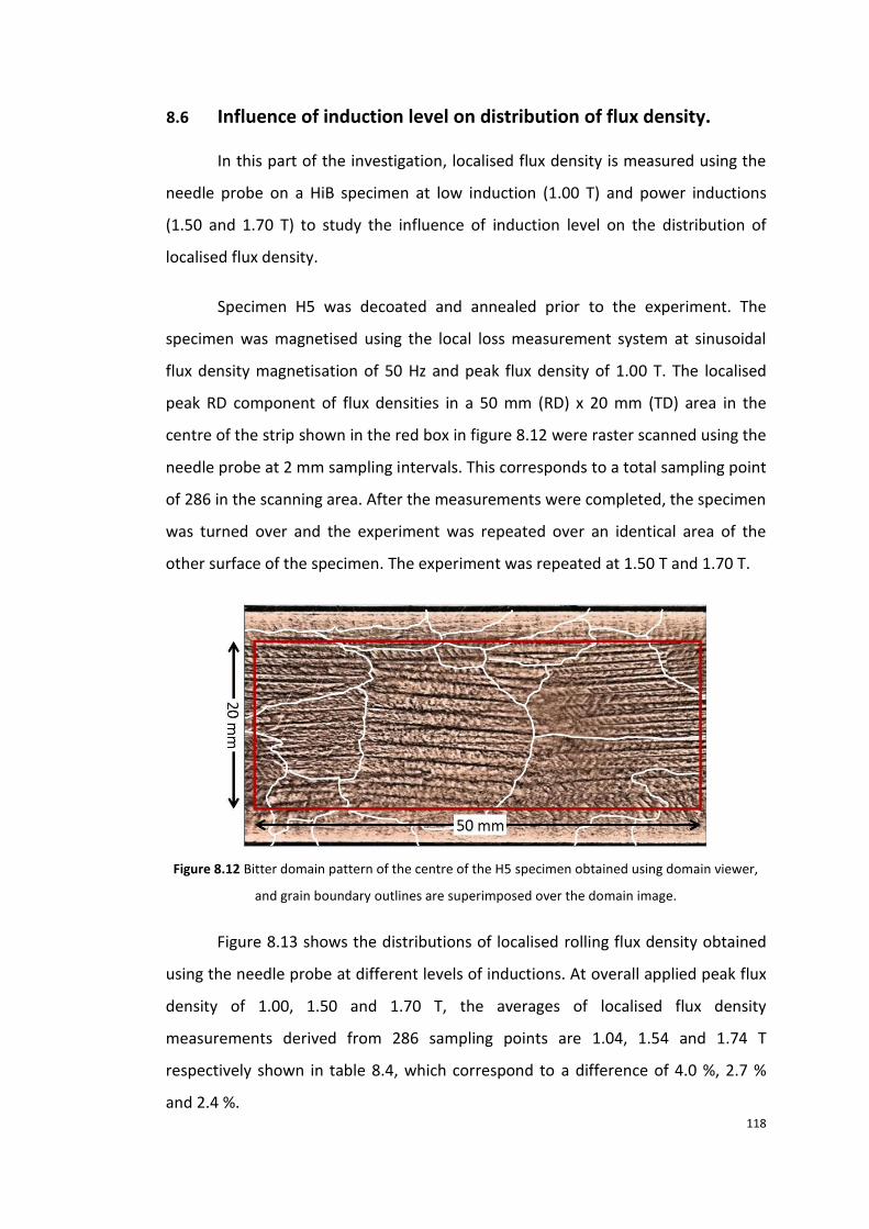
118

8.6 Influence of induction level on distribution of flux density.

In this part of the investigation, localised flux density is measured using the

needle probe on a HiB specimen at low induction (1.00 T) and power inductions

(1.50 and 1.70 T) to study the influence of induction level on the distribution of

localised flux density.

Specimen H5 was decoated and annealed prior to the experiment. The

specimen was magnetised using the local loss measurement system at sinusoidal

flux density magnetisation of 50 Hz and peak flux density of 1.00 T. The localised

peak RD component of flux densities in a 50 mm (RD) x 20 mm (TD) area in the

centre of the strip shown in the red box in figure 8.12 were raster scanned using the

needle probe at 2 mm sampling intervals. This corresponds to a total sampling point

of 286 in the scanning area. After the measurements were completed, the specimen

was turned over and the experiment was repeated over an identical area of the

other surface of the specimen. The experiment was repeated at 1.50 T and 1.70 T.

Figure 8.12 Bitter domain pattern of the centre of the H5 specimen obtained using domain viewer,

and grain boundary outlines are superimposed over the domain image.

Figure 8.13 shows the distributions of localised rolling flux density obtained

using the needle probe at different levels of inductions. At overall applied peak flux

density of 1.00, 1.50 and 1.70 T, the averages of localised flux density

measurements derived from 286 sampling points are 1.04, 1.54 and 1.74 T

respectively shown in table 8.4, which correspond to a difference of 4.0 %, 2.7 %

and 2.4 %.

119

(a) 1.00 T

(b) 1.50 T

(c) 1.70 T

Figure 8.13 Distribution of peak RD component of flux density at sinusoidal magnetisation of 50 Hz

and overall peak flux density of 1.00 T, 1.50 T and 1.70 T over the same region of specimen H5 shown

in the box in figure 8.12, and grain boundary outlines are superimposed on each contour map.

120

Boverall=1.00 T Boverall=1.50 T Boverall=1.70 T

Average of local flux density 1.04 T 1.54 T 1.74 T

Standard deviation of local flux density

7.9 % 10.6 % 11.8 %

Table 8.4 Average and standard deviation of localised flux density measurements.

It can be seen in figure 8.13 that increase in induction level leads to change

in characteristic of distribution of flux density. At lower flux density (1.00 T), as

outlined in chapter 3, flux tends to distribute along the RD of the specimen and

forms the elongated patterns. This is because less number of domain walls is

involved in the magnetisation process compare with at higher induction level,

domain walls are likely to move simultaneously on either side of grain boundary as

a result of minimisation of magnetostatic energy at grain boundaries. At higher

induction level (1.5 and 1.7 T), the magnetostatic energy profile is changed due to

domain wall refinement and banding of the 180o main domain walls, domain wall

mobility is dominantly influenced by magnetocrystalline anisotropy energy.

Therefore, flux tends to distribute more according to grain boundary outlines to

avoid relatively poorly oriented grains. As a result, lead to higher degree of variation

of localised flux density as indicated by the standard deviations shown in table 8.4.

Localised flux density at each sampling point measured at lower induction

level was subtracted from that of at higher induction level in Excel spreadsheet. It is

found that all localised flux density increases with increasing the induction level, the

rate of increasing varies from area to area. This means that the overall increase in

induction level is mainly accomplished by substantial increase in flux density in

partial areas.

Figure 8.14 shows percentage surface area of steel of flux density range. The

figure shows that localised flux densities exhibit normal distribution, which means

that localised flux densities measured in most areas of the steel are close to the

applied induction. Increase induction level is found to broaden the range of the

distribution as a result of change in characteristic of distribution of flux density and

substantial increase in localised flux density.

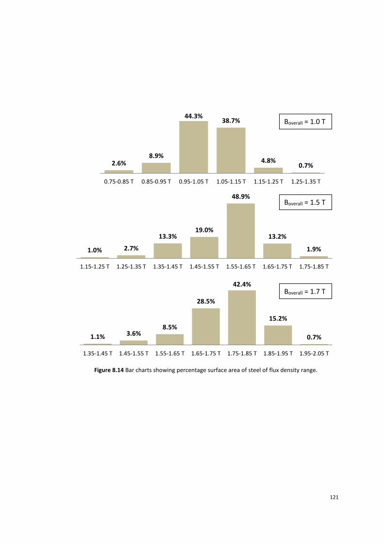
121

Figure 8.14 Bar charts showing percentage surface area of steel of flux density range.

2.6%8.9%

44.3%38.7%

4.8%0.7%

0.75-0.85 T 0.85-0.95 T 0.95-1.05 T 1.05-1.15 T 1.15-1.25 T 1.25-1.35 T

1.0% 2.7%

13.3%19.0%

48.9%

13.2%

1.9%

1.15-1.25 T 1.25-1.35 T 1.35-1.45 T 1.45-1.55 T 1.55-1.65 T 1.65-1.75 T 1.75-1.85 T

1.1% 3.6%8.5%

28.5%

42.4%

15.2%

0.7%

1.35-1.45 T 1.45-1.55 T 1.55-1.65 T 1.65-1.75 T 1.75-1.85 T 1.85-1.95 T 1.95-2.05 T

Boverall = 1.5 T

Boverall = 1.0 T

Boverall = 1.7 T

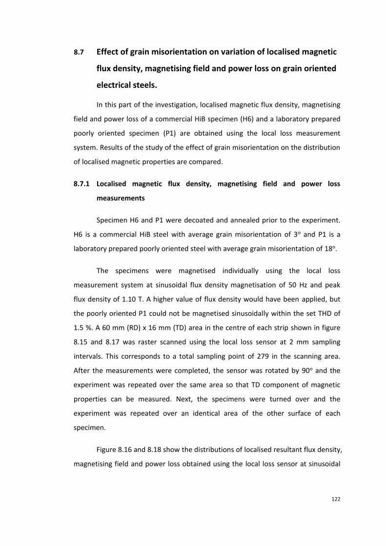
122

8.7 Effect of grain misorientation on variation of localised magnetic

flux density, magnetising field and power loss on grain oriented

electrical steels.

In this part of the investigation, localised magnetic flux density, magnetising

field and power loss of a commercial HiB specimen (H6) and a laboratory prepared

poorly oriented specimen (P1) are obtained using the local loss measurement

system. Results of the study of the effect of grain misorientation on the distribution

of localised magnetic properties are compared.

8.7.1 Localised magnetic flux density, magnetising field and power loss

measurements

Specimen H6 and P1 were decoated and annealed prior to the experiment.

H6 is a commercial HiB steel with average grain misorientation of 3o and P1 is a

laboratory prepared poorly oriented steel with average grain misorientation of 18o.

The specimens were magnetised individually using the local loss

measurement system at sinusoidal flux density magnetisation of 50 Hz and peak

flux density of 1.10 T. A higher value of flux density would have been applied, but

the poorly oriented P1 could not be magnetised sinusoidally within the set THD of

1.5 %. A 60 mm (RD) x 16 mm (TD) area in the centre of each strip shown in figure

8.15 and 8.17 was raster scanned using the local loss sensor at 2 mm sampling

intervals. This corresponds to a total sampling point of 279 in the scanning area.

After the measurements were completed, the sensor was rotated by 90o and the

experiment was repeated over the same area so that TD component of magnetic

properties can be measured. Next, the specimens were turned over and the

experiment was repeated over an identical area of the other surface of each

specimen.

Figure 8.16 and 8.18 show the distributions of localised resultant flux density,

magnetising field and power loss obtained using the local loss sensor at sinusoidal

123

magnetisation of 50 Hz and overall peak flux density of 1.10 T measured in H6 and

P1 respectively.

Figure 8.15 Grain boundary outlines superimposed on Bitter domain pattern showing the scanning area on H6.

Figure 8.16 Distribution of peak resultant flux density, magnetising field and power loss at sinusoidal magnetisation of 50 Hz and overall peak flux density of 1.10 T over the same region of H6 shown in

the box in figure 8.15, and grain boundary outlines are superimposed on each contour map.

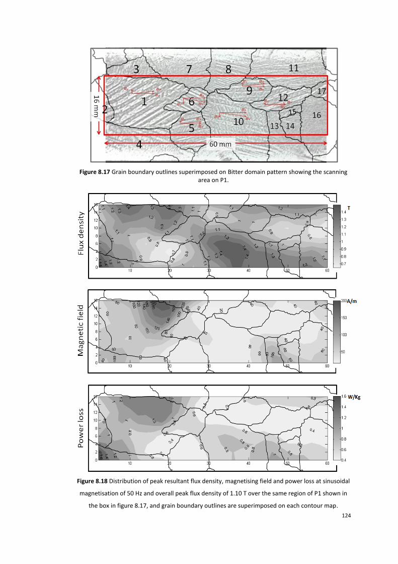
124

Figure 8.17 Grain boundary outlines superimposed on Bitter domain pattern showing the scanning area on P1.

Figure 8.18 Distribution of peak resultant flux density, magnetising field and power loss at sinusoidal

magnetisation of 50 Hz and overall peak flux density of 1.10 T over the same region of P1 shown in

the box in figure 8.17, and grain boundary outlines are superimposed on each contour map.

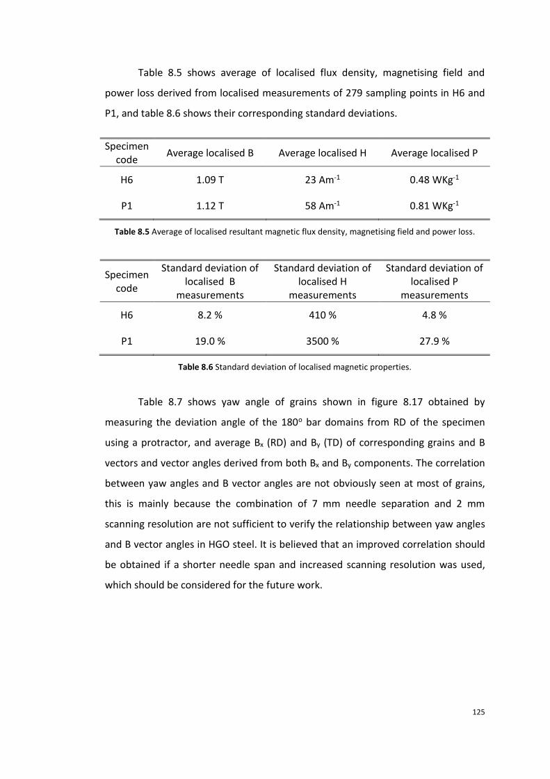
125

Table 8.5 shows average of localised flux density, magnetising field and

power loss derived from localised measurements of 279 sampling points in H6 and

P1, and table 8.6 shows their corresponding standard deviations.

Specimen code

Average localised B Average localised H Average localised P

H6 1.09 T 23 Am-1 0.48 WKg-1

P1 1.12 T 58 Am-1 0.81 WKg-1

Table 8.5 Average of localised resultant magnetic flux density, magnetising field and power loss.

Specimen code

Standard deviation of localised B

measurements

Standard deviation of localised H

measurements

Standard deviation of localised P

measurements

H6 8.2 % 410 % 4.8 %

P1 19.0 % 3500 % 27.9 %

Table 8.6 Standard deviation of localised magnetic properties.

Table 8.7 shows yaw angle of grains shown in figure 8.17 obtained by

measuring the deviation angle of the 180o bar domains from RD of the specimen

using a protractor, and average Bx (RD) and By (TD) of corresponding grains and B

vectors and vector angles derived from both Bx and By components. The correlation

between yaw angles and B vector angles are not obviously seen at most of grains,

this is mainly because the combination of 7 mm needle separation and 2 mm

scanning resolution are not sufficient to verify the relationship between yaw angles

and B vector angles in HGO steel. It is believed that an improved correlation should

be obtained if a shorter needle span and increased scanning resolution was used,

which should be considered for the future work.

126

Grain No. Yaw

angle °

Average

Bx (T)

Average

By (T)

B vector

(T) B vector angle °

1 31.00 1.08 0.15 1.09 7.83

5 16.50 0.97 0.14 0.98 8.54

6 31.50 1.08 0.27 1.11 14.55

8 16.50 1.01 0.28 1.05 16.51

9 2.50 1.05 0.14 1.05 7.55

10 12.00 1.30 0.21 1.32 9.40

11 8.50 1.24 0.06 1.24 2.74

12 16.50 0.92 0.07 0.93 4.29

13 6.50 1.31 0.21 1.32 9.29

14 4.50 1.22 0.17 1.23 8.04

15 15.00 0.95 0.09 0.95 5.44

16 6.50 1.04 0.15 1.05 8.53

17 36.00 0.92 0.10 0.93 6.13

Table 8.7 Yaw angles and B vector angles of grains shown in figure 8.17.

The resultant magnetic flux density, magnetising field and power loss

contour maps shown in figure 8.16 and 8.18 show that all the measured localised

magnetic properties in the poorly oriented P1 exhibit wider distribution range

compare to that of H6. At overall peak flux density of 1.10 T, the localised resultant

magnetic properties in P1 varies from 0.65 to 1.55 T, 20 to 200 A/m and 0.4 to 1.6

W/Kg, and in H6 varies from 0.75 to 1.35 T, 18 to 34 A/m and 0.3 to 0.7 W/Kg. In

addition, substantial increase in standard deviation of localised magnetic properties

measurements were calculated for P1 compared to H6 shown in table 8.6. The

results show that the degree of variation of localised flux density, magnetising field

and power loss increases with increasing average of grain misorientation angle.

It is considered that flux distributes itself in a such way to reduce overall

energy of the system. In H6, flux tends to distribute along RD as result of

minimisation of magnetostatic energy as discussed in 8.6. In P1, flux tends to

distribute more according to the grain outlines compared to that of H6. Grains with

easy axes closer to the RD or direction of the field are easier magnetised than

deviated grains as described by magnetocrystalline anisotropy energy outlined in

chapter 2. As a result, grains with small yaw angle should exhibit higher flux

densities than those with larger yaw angle. The relationship between average

resultant flux density measured within individual grains of P1 and the yaw angles of

127

the individual grains is shown in figure 8.19. The trend line shows that the average

resultant flux density in individual grains decreases with increasing yaw angle. The

relationship between average flux density and yaw angle was not obvious as the

calculated correlation coefficient for the trend line was -0.26. This is because that

the distribution of flux density is not only influenced by grain orientation but also

the local grain arrangement. At the bottom right corner of grain 1, where grain

boundary is shared with grain 4, 5 and 6 shown in figure 8.17, the lowest flux

density was measured compared to the other area shown in figure 8.18. This is

considered due to an enhanced effect of large yaw angle and mismatched grain

arrangement. A detailed study is presented in 8.7.2, where the DC domain wall

movement in grain 1 was observed while investigating the large variation of flux

density within the grain.

Figure 8.19 Relationship between localised resultant flux density measured within grains of P1 and

yaw angles of the grains.

The variation of localised magnetising field can be explained by the existence

of the localised demagnetising field. The result of domain observation presented in

8.3 shows that creation of flux closure domains did not occur at grain boundary of

0.8

0.9

1

1.1

1.2

1.3

1.4

1.5

0 5 10 15 20 25 30 35 40

Ave

rage

res

ult

ant

flu

x d

ensi

ty m

eau

sred

wit

hin

in

div

idu

algr

ain

s o

f P

1 (

T)

Yaw angle of individual grains in P1 (°)

128

discontinued 180o domains, which indicates that there is a demagnetising field as a

result of exposure of free magnetic pole at grain boundaries. In H6, the 180o domain

walls mostly move simultaneously in adjacent grains as indicated by the elongated

distribution pattern as discussed in 8.6. Consequently, this lead to a lower

demagnetising field at grain boundaries, thus the surface magnetising field

measured on H6 varies considerably less than that on P1. In P1, flux distributes

more according to grain outlines, which means that the correlation of 180o domain

wall movements in adjacent grains is not as close as that in H6 as a result of the

increased grain misorientation and grain mismatch angle. This increases the

localised demagnetising field, which in combination with the higher field strength

needed for excitation P1 to the same induction level than that for H6 (indicated by

the average of localised magnetising field shown in table 8.5), causes the higher

degree of variation of localised magnetising field.

Comparison of flux density, magnetising field and power loss distribution

patterns shown in figure 8.16 and 8.18 indicates that the localised loss distribution

is influenced by both flux density and magnetising field. The average of localised

power loss of 0.48 and 0.81 W/Kg is calculated for H6 and P1 respectively shown in

table 8.5. The high loss value measured in P1 is believed mainly due to the great

average resultant localised flux density and magnetising field and larger degree of

their variations occur in the poorly oriented specimen.

Figure 8.20a and 8.20b show the distribution of the TD component of flux

density measured over the same area shown in the boxed areas in figure 8.15 and

8.17 respectively. Obviously, the TD component of flux density in P1 shows greater

magnitude and higher level of variation than that in H6. The average of the localised

TD component of flux density of P1 is more than double that of H6 shown in table

8.8, and the corresponding standard deviation reveals that the degree of variation

of the TD component of flux density in P1 is almost twice as high as that in H6. The

results confirm that there is definite correlation between the TD component of flux

density and the average grain misorientation.

129

Figure 8.21 shows the relationship between the average TD component of

flux density measured within individual grains of P1 and the yaw angles of the

individual grains. Despite the large scattered data, which is believed to be caused by

the local variation of the resultant flux density, the average TD component of flux

density in individually grains increases with increasing yaw angle as indicated by the

best-fit trend line. This confirms that the TD component of flux density is mainly a

result of change in y component of flux density due to movement of the 180o

domain walls parallel to the [100] directions of individual grains.

(a) H6

(b) P1

Figure 8.20 Distribution of peak TD component of flux density at sinusoidal magnetisation of 50 Hz and overall peak flux density of 1.10 T, and grain boundary outlines are superimposed on each

contour map.

Specimen code Average localised TD

component of flux density Standard deviation

H6 0.06 T 4.5 %

P1 0.16 T 8.0 %

Table 8.8 Average localised TD component of flux density and standard deviation.

130

Figure 8.21 Relationship between localised TD component of flux density measured within grains of

P1 and yaw angles of the grains.

0

0.05

0.1

0.15

0.2

0.25

0.3

0.35

0 5 10 15 20 25 30 35 40

Ave

rage

TD

co

mp

on

enet

of

flu

x d

ensi

ty m

easu

red

wit

hin

ind

ivid

ual

grai

ns

of

P1

(T)

Yaw angle of individual grains in P1 (°)

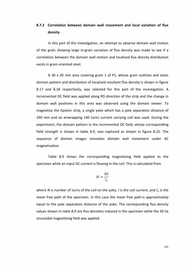
131

8.7.2 Correlation between domain wall movement and local variation of flux

density

In this part of the investigation, an attempt to observe domain wall motion

of the grain showing large in-grain variation of flux density was made to see if a

correlation between the domain wall motion and localised flux density distribution

exists in grain oriented steel.

A 30 x 30 mm area covering grain 1 of P1, whose grain outlines and static

domain pattern and distribution of localised resultant flux density is shown in figure

8.17 and 8.18 respectively, was selected for this part of the investigation. A

incremented DC field was applied along RD direction of the strip and the change in

domain wall positions in this area was observed using the domain viewer. To

magnetise the Epstein strip, a single yoke which has a pole separation distance of

290 mm and an enwrapping 140 turns current carrying coil was used. During the

experiment, the domain pattern in the incremented DC field, whose corresponding

field strength is shown in table 8.9, was captured as shown in figure 8.22. The

sequence of domain images simulates domain wall movement under AC

magnetisation.

Table 8.9 shows the corresponding magnetising field applied to the

specimen while an input DC current is flowing in the coil. This is calculated from

𝐻 =𝑁𝐼

𝑙𝑠

where N is number of turns of the coil on the yoke, I is the coil current, and 𝑙𝑠 is the

mean free path of the specimen. In this case the mean free path is approximately

equal to the pole separation distance of the yoke. The corresponding flux density

values shown in table 8.9 are flux densities induced in the specimen while the 50 Hz

sinusoidal magnetising field was applied.

132

Input current (A) Magnetising field (A/m) Magnetic flux density (T)

0.00 0 0.00 0.05 24 0.70 0.10 48 1.05 0.15 72 1.24 0.20 96 1.31 0.25 120 1.35

Table 8.9 The corresponding magnetising field and flux density at the input currents.

Figure 8.22 Static domain patterns obtained using the domain viewer showing domain wall position

in an incremented DC field, and the area of view is 30 mm x 30 mm covering grain 1 of P1. (a) 0.00 T,

(b) 0.70 T, (c) 1.05 T, (d) 1.24 T, (e) 1.31 T and (f) 1.35 T. The direction of RD and DC field is along the

horizontal axis.

The sequence of DC domain patterns shown in figure 8.22 simulates domain

wall movement in an increasing magnetising field from 0 to 120 A/m or 0 to 1.35 T.

Domains within grain 1 respond differently to the external field. At lower fields (see

figure 8.22 b and c), domains in the top right corner start to reconfigure by growing

black domains whose RD components of magnetisation are aligned in the field

direction, and domains in the rest of the area in grain 1 remain almost unchanged.

On further increase of field (see figure 8.22 d), domains that are in connection with

grain 2 and 3 start to reconfigure. At higher fields (see figure 8.22 e and f), only a

1

7

6

4

5

3

2

133

small fraction of domains at the bottom right corner remains unchanged while the

rest of the area in grain 1 are being magnetised as a single black domain. Comparing

the DC domain patterns presented in figure 8.22 and distribution of localised

resultant flux density shown in figure 8.18. It is found that the area showing early

domain reconfiguration exhibit higher flux density compared to other areas, and the

area showing the least domain reconfiguration throughout the magnetisation

process exhibits the lowest flux density. This result shows that there is strong

correlation between characteristic of domain wall movement and distribution of

localised flux density.

The large in-grain variation of flux density found in grain 1 is believed to be

influenced by local grain arrangement and grain geometry. When an external

magnetising field is applied in the RD direction of the specimen, it can be assumed

that 180o domain walls in relatively less deviated grains are more mobile than those

in largely deviated grains, thus domain walls in the surrounding grains 2 to 7 are

expected respond differently in the applied external field. In the vicinity of the grain

boundary between grain 1 and 2, assume domain walls in the relatively less

deviated grain 2 moves first under the applied field, then free magnetic poles are

exposed at the boundary, which increases the magnetostatic energy. The rise of

magnetostatic energy is then lowered by moving the corresponding domain walls in

grain 1 to match with walls in grain 2. In this case, the higher flux density measured

within grain 1 in the vicinity of the grain boundary is mainly due to the interaction

of domain walls of the adjacent grains. At the bottom right corner of the grain 1,

where the least domain wall movement are observed, wall migration is less

energetically favourable in this area as it can lead to significant increase in

magnetostatic energy due to large grain mismatch angles. In addition, due to the

grain geometry, demagnetising field factor at both top left corner and bottom right

corner is higher compared to the middle section of the grain. This should also lead

walls at corners move less active than in the middle of the large grain as observed in

figure 8.22.

134

8.8 Effect of domain refinement on distribution of local magnetic

flux density of HiB electrical steel.

Domain refinement is an important method for reducing power loss of HiB

electrical steels. In this part of investigation, localised flux density of a HiB specimen

before and after domain refinement was measured using the local loss

measurement system to study the effect of domain refinement on the distribution

of localised magnetic flux density.

Specimen H7 was decoated and annealed prior to the experiment. Domain

wall spacing of the specimen was then refined by means of ball scribing using a

weighted ballpoint pen at 90o to the RD on one surface of the specimen. The ball

scribing was carried out at intervals of 12 mm, 6 mm and 3 mm respectively.

Magnetic domain patterns before and after ball scribing were inspected using the

domain viewer and as shown in figure 8.23, the average domain wall spacing shown

in table 8.10 was derived from,

Average of wall spacing =width of the speicmen x 3

Number of domains counted in three columns (mm)

The overall power loss and average of AC relative permeability of the

specimen before and after ball scribing were measured using a single strip tester at

sinusoidal magnetisation of 50 Hz and a range of peak flux density from 1.00 T to

1.70 T. Results are shown in figure 8.24 and 8.25 respectively. The localised RD

component of flux density before and after ball scribing was measured using the

local loss measurement system at sinusoidal flux density magnetisation of 50 Hz and

peak flux density of 1.70 T. To avoid the influence of high surface leakage field

produced by free magnetic poles at the scribed grooves on the accuracy of NP, the

scribed surface of the specimen faced downwards and the localised peak RD

component of flux density in a 60 mm (RD) x 20 mm (TD) area in the centre of the

strip and on the other surface was raster scanned using the NP at 2 mm sampling

intervals.

135

(a)

(b)

(c)

(d)

Figure 8.23 Magnetic domain patterns obtained using the domain viewer over the centre area of H7

(a) Unscribed, (b) 12 mm scribed, (c) 6 mm scribed and (d) 3 mm scribed.

Scribe spacing (mm) Average domain wall spacing (mm)

Un-scribed 0.96 12 0.85 6 0.55 3 0.36

Table 8.10 Average domain wall spacing.

136

Figure 8.24 Relationship between power loss and flux density.

Figure 8.25 Relationship between average of the AC relative permeability and flux density.

0.4

0.6

0.8

1

1.2

1.4

1 1.1 1.2 1.3 1.4 1.5 1.6 1.7

Po

wer

loss

(W

/Kg)

Peak flux density (T)

unscribed12 mm spacing6 mm spacing3 mm spacing

6.00E+03

8.00E+03

1.00E+04

1.20E+04

1.40E+04

1 1.1 1.2 1.3 1.4 1.5 1.6 1.7

Ave

rage

of

the

AC

rel

ativ

e p

erm

eab

ility

Peak flux density (T)

unscribed12 mm spacing6 mm spacing3 mm spacing

137

Figure 8.24 shows the relationship between overall power loss and peak flux

density for the specimen before scribing, and after scribing at 12 mm, 6 mm and 3

mm spacing respectively obtained using the single strip tester. It is seen that the

specimen after scribing exhibit reduced power loss compared to that of before

domain scribing, the highest loss reduction over the entire studied flux density

range of 1.00 to 1.70 T is found at 6 mm spacing. At peak flux density below 1.20 T,

the loss curves of the 6 mm and 3 mm spacing show similar trends and loss values,

but at peak flux densities above 1.20 T, the slope of the 3 mm curve exhibits sharper

increase than that of other curves. Above 1.4 T, the 3 mm curve overtakes 12 mm

curve and the loss of the 3 mm spacing becomes the highest of all scribing spacing.

Figure 8.25 shows the relationship between the average of the AC relative

permeability and the peak flux density for the specimen before scribing and after

scribing at 12 mm, 6 mm and 3 mm spacing respectively obtained using the single

strip tester. All curves exhibit similar trends, the average of the AC relative

permeability increases with increasing flux density, then decreases at higher flux

density, but the change in trend occurs at different peak flux density values. The

change in trend occurs at a lower peak flux density in the specimen after scribing

than before scribing. At lower flux densities (< 1.20 T), the averages of the AC

relative permeability of the specimen after domain scribing is higher than that

before scribing, and increases with decreasing scribing spacing. At higher flux

densities (>1.65 T), the averages of the AC relative permeability of the specimen

after scribing is lower than before scribing, and decreases with decreasing scribing

spacing.

Domain refinement by means of ball scribing reduces AC power loss of

electrical steel as a result of decreasing the eddy current loss due to decreasing the

mean free path of domain walls as shown in table 8.10. However, the method of

domain scribing introduces residual stresses which act as domain wall pinning and

increases hysteresis loss. At lower flux density, domain walls propagate shorter

distance hence encounter fewer pinning sites. At higher flux density, domain walls

propagate longer distance and have to encounter more pinning sites leading to

138

increased hysteresis loss and decreased permeability compared to that at lower flux

density. Excessive scribing in a confined area (i.e. domain scribing at 3 mm spacing)

leads to reasonable decrease of eddy current loss but substantially increase in

hysteresis loss. Therefore, the optimum loss reduction is found to be at the

moderate 6 mm spacing.

Figure 8.26 shows the distribution of the RD component of flux density of

specimen H7 before and after scribing obtained using NP on one surface of the

specimen. Comparison of the contour maps indicates that there is an obvious

change in flux distribution. No correlation is found between scribing line positions

and flux distribution. The specimen after scribing shows a narrower flux density

distribution range as indicated by the percentage area of steel of flux density range

shown in figure 8.27. The standard deviation of the localised flux density

measurements decreases with decreasing scribing spacing as shown in table 8.11.

The results indicate that domain scribing improves the uniformity of flux density

distribution.

139

(a) Unscribed

(b) 12 mm spacing

(c) 6 mm spacing

(d) 3 mm spacing

Figure 8.26 Distribution of peak RD component of flux density obtained using NP at sinusoidal

magnetisation of 50 Hz and overall peak flux density of 1.7 T over 60 mm x 20 mm area on the other

surface which is opposite to the scribing surface of H7, and scribe line positions are shown by the

white lines.

(mm)

(mm)

(mm)

(mm)

(mm)

(mm)

(mm)

(mm)

(T)

(T)

(T)

(T)

140

Figure 8.27 Bar charts showing percentage area of steel of flux density range.

Unscribed 12 mm spacing 6 mm spacing 3 mm spacing

Average of localised B 1.68 T 1.71 T 1.72 T 1.81 T

Standard deviation of localised B

14 % 12 % 10 % 7 %

Table 8.11 Average and standard deviation of local flux density measurements.

0.3% 2.9% 2.9%10.6%

17.3%

31.1%26.4%

7.6%0.9%

1.15-1.25 T 1.25-1.35 T 1.35-1.45 T 1.45-1.55 T 1.55-1.65 T 1.65-1.75 T 1.75-1.85 T 1.85-1.95 T 1.95-2.05 T

Unscribed

0.0% 0.0% 3.2% 4.1%

25.5%31.1%

24.6%

10.6%

0.9%

1.15-1.25 T 1.25-1.35 T 1.35-1.45 T 1.45-1.55 T 1.55-1.65 T 1.65-1.75 T 1.75-1.85 T 1.85-1.95 T 1.95-2.05 T

12 mm spacing

0.0% 0.0% 0.3%5.6%

16.7%

36.7%32.6%

7.9%0.3%

1.15-1.25 T 1.25-1.35 T 1.35-1.45 T 1.45-1.55 T 1.55-1.65 T 1.65-1.75 T 1.75-1.85 T 1.85-1.95 T 1.95-2.05 T

6 mm spacing

0.0% 0.0% 0.0% 0.0% 3.2%

13.8%

55.1%

27.3%

0.6%

1.15-1.25 T 1.25-1.35 T 1.35-1.45 T 1.45-1.55 T 1.55-1.65 T 1.65-1.75 T 1.75-1.85 T 1.85-1.95 T 1.95-2.05 T

3 mm spacing

141

A substantial increase in the average localised flux density is found in the

specimen after scribing at 3 mm spacing shown in table 8.11. At peak overall flux

density of 1.70 T, the average localised flux density measurements derived from 341

localised sampling points is 1.81 T, which correspond to a difference of 6.5 %. Such

a large difference between overall flux density and averaged localised flux density is

not found for the other scribing spacing as studied here. It should be noted that in

this part of the investigation, localised flux density results were obtained from

single surface NP measurements, the average difference between NP

measurements obtained on a single surface and the average of both surfaces of HiB

steel is estimated to be less than 1.9 % (see in 8.4). Even taking into account the 1.9 %

difference, the difference of 6.5 % is still considerably high compared to the 2.4 %

measured on the other HiB specimen at the same overall peak flux density as

outlined in 8.6. This difference is assumed to be caused by non-uniform distribution

of flux density in the thickness direction of the specimen due to non-uniform

distribution of applied stresses as a result of scribing with the weighted ballpoint

pen.

Figure 8.28 shows a simple illustration of the stress profile of the after

scribed specimen based on the results obtained by Fukawa [8.3]. It can be seen that

compressive stress is distributed mainly around the scribe traces as indicated by C1

zone and below C1 zone on the other side as indicated by C2 zone; tensile stress as

indicated by T zone is distributed mainly to the remaining volume of the material. It

can be assumed that 180o domain walls in tensile zone are more mobile than those

in compressive zones, because when grain oriented steel is subjected to tensile

stress the increase of 180o domains at expense of the surface 90o domains becomes

energetically favourable due to shift of the magnetic easy axis towards the direction

of applied stress [8.4], while subjected to compressive stress the decrease of 180o

domains at growth of the surface 90o domains becomes energetically favourable.

Therefore, steel under tensile stress are easier magnetised that under compressive

stress since magnetisation in the presence of an AC field applied parallel to the RD is

mainly by 180o wall motion parallel to the easy direction.

142

Excessive scribing in a confined area leads to increased stress polarisation in

the direction of the specimen’s thickness as shown in figure 8.28b, which increases

the differences in flux density induced in either side of the steel.

Figure 8.28 Illustration of stress distribution in domain scribed specimen.

To verify the proposed theory, the specimen after scribing at 3 mm spacing

was turned over and localised peak RD component of flux density in the 60 mm x 20

mm identical area on the scribed surface was raster scanned using the local loss

measurement system at the same overall magnetisation of 50 Hz and peak overall

flux density of 1.70 T. The distribution of flux density obtained using the NP in the

scribing side and non-scribing side of the specimen scribed at 3 mm spacing are

compared in figure 8.29. It can be seen that the flux densities obtained at identical

area are relatively smaller using the scribing side compared to those using the non-

scribing side. Localised flux density is found to vary in a range from 1.35 T to 1.75 T

and from 1.65 T to 2.05 T using the scribing and non-scribing side respectively for

the measurement, and the corresponding averaged localised flux density is 1.56 T

and 1.81 T as shown in table 8.12. The results confirm that there is a large

difference in flux density induced in either side of the specimen scribed at 3 mm

spacing. This increases the degree of non-uniformity of distribution of localised flux

density, which together with the increased hysteresis loss is considered to be the

reasons for the higher loss found in the 3 mm spacing shown in figure 8.24.

Further research could be carried out by observing dynamic domain on both

surfaces of the steel after scribing to improve understanding of the influence of

applied stress on the dynamic domain configuration, and to look for any correlation

143

between characteristics of dynamic domain wall movement and localised flux

density.

(a) Scribing side

(b) Non-scribing side

Figure 8.29 Distribution of peak localised RD component of flux density measured in identical area in

both sides of the specimen scribed at 3 mm spacing.

Scribing side Non-scribing side

Average of local flux density

1.56 T 1.81 T

Table 8.12 Average of localised flux density.

(mm)

(mm) (T)

(mm)

(mm) (T)

144

References

[8.1] X. Xu, A. Moses, J. Hall, P. William and K. Jenkins, “A comparison of magnetic

domain images using a modified Bitter pattern technique and the Kerr

method on grain-oriented electrical steel”, IEEE Transactions on Magnetics,

vol. 47, pp. 3531 – 3534, (2011).

[8.2] G. Loisos and A. J. Moses, “Critical evaluation and limitations of localized flux

density measurements in electrical steels”, IEEE Transactions on Magnetics,

vol. 37, pp. 2755 – 2757, (2001).

[8.3] K. Fukawa and T. Yamamoto, “Domain structures and stress distribution due

to ball-point scratching in 3% Si-Fe single crystals with orientation near

(110)[001]”, IEEE Transactions on Magnetics, vol. 18, pp. 963-969, (1982).

[8.4] T. W. Krause, L. Clapham, A. Pattantyus and D. L. Atherton, “Investigation of

the stress-dependent magnetic easy axis in steel using magnetic Barkhausen

noise”, Journal of Applied Physics, vol. 9, pp. 4242 – 4252, (1996).

145

Chapter 9

Conclusions

Both domain viewer and magneto-optical Kerr microscope can provide

important information with regard to magnetic domain configuration and crystal

orientation of grain oriented electrical steel. The domain viewer is found more

sensitive to small angle grain boundary than the Kerr microscope. However, the

image contrast cannot be relied upon to determine the absolute direction of

domain magnetisation since it is an indirect domain observation method. The Kerr

microscope is found more sensitive to domain magnetisation than the domain

viewer, but the equally important small angle grain boundary was not observed

using the Kerr microscope since the overall magnetisation continues across the

boundary. This finding would be useful in providing accurate analysis on domain

images obtained using any stray field sensitive method and the magnetisation

polarisation method.

The real time dynamic domain patterns captured using the Kerr microscope

showed that the 180o walls are not moving homogeneously and consistently at the

vicinity of the grain boundary under AC magnetisation, which proves the existence

of the local non-uniform magnetisation.

A local loss measurement sensor, which comprises a Needle Probe (NP) and

Hall Effect sensor, was made for measurement of localised magnetic flux density,

magnetising field and power loss of grain oriented electrical steel. The uncertainties

146

of flux density, magnetising field and power loss measurements are evaluated to be

±0.22 %, ±1.09 % and ±1.76 % respectively. Flux density measured using NP and

search coil respectively at identical positions on a high permeability grain oriented

steel (HiB) were in good agreement, which gives a high degree of confidence in the

localised flux density measurements.

Localised flux density of grain oriented electrical steel are found to vary

greatly under AC magnetisation of 50 Hz. Increasing induction level or grain

misorientation changes the characteristic of distribution of flux density. At a lower

induction and grain misorientation, magnetostatic energy dominates flux

distribution, flux tends to distribute along rolling direction of the specimen as in this

way to minimise the magnetostatic energy. At a higher induction or grain

misorientation, both magnetostatic and magnetocrystalline anisotropy energy

dominate flux distribution, flux tends to distribute more according to grain outline

compared to that at lower induction and grain misorientation, as a result, leading to

increased degree of variation of flux density. A strong correlation between domain

configuration and localised flux density distribution is found showing the main

causes of the variation of flux density are due to the grain misorientation and the

local grain arrangement. The transverse component of flux density is detected and

is found increases with increasing grain misorientation.

The variation of localised magnetising field is found to be influenced by the

localised demagnetising field that is generated by free magnetic poles at grain

boundaries of the discontinued magnetisation.

Comparison of localised flux density, magnetising field and power loss

distribution maps showed that the distribution of localised power loss is strongly

influenced by both the localised flux density and magnetising field.

Domain refinement by means of ball scribing on one surface of HiB steel at

90o to the RD is found to influence the characteristic of flux density distribution. At

12 mm and 6 mm scribing spacing, result showed that the ball scribing can improve

the uniformity of distribution of localised flux density and reduce the overall power

147

loss of the steel. At 3 mm scribing spacing, result inferred that the stress

polarisation due to the ball scribing could lead to obvious uneven distribution of flux

density in the direction of the specimen’s thickness and increased power loss.

Future investigation

This investigation has indentified the need for future research in helping to

improve the understanding of the causes of the non-uniform magnetisation:

The future work would be to repeat the investigation on conventional grain

oriented steel or different degree of misoriention steel to quantify the

influence of misorientation on variation of localised magnetic properties of

electrical steels.

Dynamic domain observation at 50 Hz on both surfaces of the domain refined

steel should be investigated to look for any correlation between the

characteristic of domain wall movements and the differences in flux density

induced in either side of the steel.