local variance gamma option pricing model - kth · i we note that this pdde arises if rothe’s...

Local Variance Gamma Option Pricing Model

Peter Carr

Bloomberg/Courant Institute

April 28, 2009

P. Carr Local Variance Gamma

Automated Option Market Making

I As markets move from an open outcry system to computerizedexchanges, the question arises as to how to automate thepricing and risk management of derivative securities.

I We take the view that this problem is presently unsolved andthis explains why firms continue to use traders to price andhedge.

I The true “revenge of the nerds” will begin when a quantdevelops a solution to this problem.


First Statement of The Problem

I Banks,software vendors, and other options market participantshave historically hired armies of PhD’s to tackle the followingapparently simple problem.

I Problem Statement:Given the current market price of theunderlying asset and also given market option quotes atseveral given strikes and terms, provide options quotes at anystrike and term in a specified set.

I For simplicity, we suppose that both the supplied quotes andthe produced quotes are mid-points of the bid and the ask.

I For simplicity, we suppose that both the input quotes and theoutput quotes are for European options.

I We will refer to the given strikes, terms, and mids as “listed”.The problem of inferring option prices at non-listed strikes andterms arises on both exchanges and OTC.


How Many PhD’s Does it Take to Connect the Dots?

I Since the supplied mids can be depicted as points in the firstoctant of R3, it first appears that armies of PhD’s are merelybeing asked to connect the dots.

I As my 7 year old daughter mastered this intellectual challengeseveral years ago, one has to wonder if this is not the financialequivalent of the lightbulb joke.

I It is my contention that once all the desired properties of thesolution are clarified, no one has ever published a solution thatsuccessfully connects the dots.


Glorified Interpolation?

I Recall that the option market-makers’ pricing problem onlyasks that option prices be provided for strikes and terms in aspecified set.

I When this set lies in the convex hull of listed strikes andterms, the option market makers pricing problem can beproperly described as “glorified interpolation”.

I When at least part of the desired set lies beyond listed strikesand terms, extrapolation is involved. Philosophically, there isno unique solution to any extrapolation problem.

I What makes this problem even more difficult is that there is along laundry list of desirable properties that a solution is askedto possess. Unfortunately, these properties are typically onlydiscovered after much effort has been spent solving the wrongproblem.


A Partial List of Desirable Properties

I The following highly demanding criteria can usually beexpressed in any of several mathematically equivalent spaces.Common spaces used for the output include option pricespace, implied vol space, and local vol space. For simplicity,we treat the independent variables as strike K and term T .

I robust to input data, i.e. desirable output is produced nomatter what is input.

I well-posedness, i.e. small changes in inputs lead only to smallchanges in output.

I locality, i.e. a small change in one input has only a local effecton the output.

I ability to accept related inputs eg. American options, varianceswaps, CDS, options on other underlyings.


A Partial List of Desirable Properties (Con’d)

I no model-free arbitrages in the output (assuming wide supportfor possible levels of the underlying uncertainty).

I exact price consistency with given mids (implied by above).

I smooth output (except for option prices at T = 0).

I perfect out-of-sample prediction in K,T space.

I ability to extrapolate in S, t space i.e., can produce deltas,gammas, thetas, spot slides, and time slides.

I resonance with financial orthodoxy eg. nonnegative gammas.



I perfect out-of-sample prediction in the Cartesian product ofspot prices S and calendar time t.

I internal consistency eg. quantitities assumed constant in aparametric model should not vary with S, t or otherobservables.

I real-time computational speed.

I numerical robustness (always works on finite precisioncomputers).



I ability to uniquely and accurately price related derivativessuch as American options, variance swaps, barrier options, andother exotics.

I parsimony

I distinct economic role for parameters that permitidentification.

I implied Q dynamics not ridiculously far from observable Pdynamics - no stat. arb.


Origin and Motivation

I Local Variance Gamma (henceforth LVG) is a work in progresswhich satisfies many, but not all, of the criteria justmentioned. The model takes its name from the fact that itsimultaneously generalizes both Dupire’s 1994 Local Variancemodel and Madan and Seneta’s 1990 Variance Gamma model.

I The use of the word “local” in the LVG name is apt for tworeasons:

1. As in local vol models, the uncertainty in stock returns isassumed to depend (only) on the stock price level and time.

2. Calibration is local, if N option prices are given, one does Nunivariate searches, rather than one global search for Nparameters.


Inputs and Outputs of LVG

I The input into LVG is any set of arbitrage-free option prices atdiscrete strikes and maturities on a regular grid. The output isan exactly-consistent arbitrage-free price process for theunderlying asset.

I Others have also done this; what is special about LVG AFAIKis that calibration to discrete strike and maturity option pricesis local and yet the produced dynamics for the underlyingasset price evolve in cont. time with a cont. state space.


Dynamical Description in Words

I In LVG, the underlying forward price process is assumed to bea driftless diffusion running on an independent gamma clock.The resulting continuous-time price process is a pure jumpMarkov martingale with infinite activity.

I The LVG price process is not a Levy process, but it enjoystime & space homogeneity between listed strikes & terms.

I If option prices at just 1 term are given, the process istime-homogeneous.

I Likewise, if option prices at just 1 strike per term are given,the process is space-homogeneous (given by time-dependentVG).

I When 2 or more option prices at 1 term or strike are given, thediffusion coefficient is assumed to be piecewise constant, i.e,it jumps at listed strikes and maturities, but is otherwise flat.


Assumptions

I In this presentation, I will just show the case where optionprices at a single term are given.

I Furthermore, interest rates and dividends are zero and limitedliability is not respected. (all of this can be relaxed).


Dynamical Description in Symbols

I Let D be a time homogeneous diffusion starting at S0:

dDs = a(Ds)dWs, s ≥ 0,

where the diffusion coefficient a(x) : R 7→ R is initiallyunspecified.

I Let {Γt, t > 0} be an independent gamma process with Levy

density kΓ(t) = e−αt

t∗t , t > 0 for parameters t∗ > 0 and α > 0.

I The marginal distribution of a gamma process at time t ≥ 0 isa gamma distribution with PDF:

Q{Γt ∈ ds} =αt/t

∗

Γ(t/t∗)st/t

∗−1e−αs, s > 0, α > 0, t∗ > 0.


Specifying the Gamma Process

I Recall that the marginal distribution of a gamma process attime t ≥ 0 is a gamma distribution with PDF:

Q{Γt ∈ ds} =αt/t

∗

Γ(t/t∗)st/t

∗−1e−αs, s > 0, α > 0, t∗ > 0.

I We set the parameter α = 1t∗ , so that the gamma process

becomes unbiased, i.e. EQΓt = t for all t ≥ 0.

I The PDF of the unbiased gamma process Γ at time t ≥ 0 is:

Q{Γt ∈ ds} =st/t

∗−1e−s/t∗

(t∗)t/t∗Γ(t/t∗), s > 0,

for parameter t∗ > 0.

I When t = t∗, this PDF is exponential. We choose t∗ to be thegiven term, so that the distribution of the gamma clock atexpiry is exponential.


Local Variance Gamma Process

I We assume that the underlying spot price process S isobtained by subordinating the driftless diffusion D to theunbiased gamma process Γ:

St = DΓt , t ≥ 0.

I S inherits the local martingale property from the diffusion D.

I S inherits dependence of its increments on its level from D.

I S inherits jumps from the gamma process Γ.

I S inherits time homogeneity from D and Γ.


Forward PDDE

I Define C(S, T,K) as the value of a European call with stockprice S ∈ R, term T ≥ 0, and strike K ∈ R in the LVG model.

I Then it can be shown that the LVG model value satisfies thefollowing forward PDDE:

C(S, T + t∗,K)− C(S, T,K)t∗

=a2(K)

2∂2

∂K2C(S, T + t∗,K),

for all S ∈ R, T ≥ 0, and K ∈ R.

I Remarkably, the effect of the gamma time change is tosimultaneously inject realism into the underlying pricedynamics and to semi-discretize Dupire’s forward PDE.

I More specifically, Dupire’s infinitessimal calendar spread getsreplaced by a discrete calendar spread, with the time betweenthe two maturities given by t∗.


Forward PDDE (Con’d)

I Setting the first maturity date to the valuation date andS = S0, the LVG model value of a call satisfies:

C(S0, t∗,K)− (S0 −K)+

t∗=a2(K)

2∂2

∂K2C(S0, t

∗,K),

for all K ∈ R.

I If call prices at a continuum of strikes are given, then thediffusion coefficient a(x) becomes observed.

I As a result, the stock price process becomes specified.Options of other terms and other derivatives can be valued byMonte Carlo.


Backward PDDE

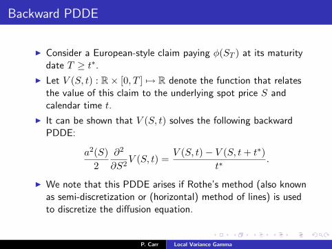
I Consider a European-style claim paying φ(ST ) at its maturitydate T ≥ t∗.

I Let V (S, t) : R× [0, T ] 7→ R denote the function that relatesthe value of this claim to the underlying spot price S andcalendar time t.

I It can be shown that V (S, t) solves the following backwardPDDE:

a2(S)2

∂2

∂S2V (S, t) =

V (S, t)− V (S, t+ t∗)t∗

.

I We note that this PDDE arises if Rothe’s method (also knownas semi-discretization or (horizontal) method of lines) is usedto discretize the diffusion equation.


Backward PDDE (Con’d)

I The European claim value function V satisfies the terminalcondition:

V (S, T ) = φ(S), S ∈ R.

I Re-arranging the backward PDDE implies that V (S, t) solvesthe following second order inhomogeneous ODE:

t∗a2(S)

2∂2

∂S2V (S, t)− V (S, t) = −V (S, t+ t∗).

I Evaluating at t = T − t∗ the RHS forcing term is φ(S). Onecan numerically solve the ODE and recursively step backwardsin time steps of length t∗.

I The algorithm switches from the express (ODE) to the local(PIDE), when the express would overshoot the valuation time.


Discrete Strikes

I Setting T = 0 and S = S0 in the forward PDDE, the LVGmodel value of a call solves a linear second order ODE in K:

t∗a2(K)

2∂2

∂K2C(S0, t

∗,K)− C(S0, t∗,K) = −(S0 −K)+

for all K ∈ R.

I If call prices at only a finite number of strikes are given, thenwe can no longer determine the a function explicitly.

I As the next best thing, we assume that the diffusioncoefficient a is piecewise constant. As a result, between any 2adjacent strikes, the linear 2nd order ODE has constantcoefficients and given Dirichlet boundary conditions.

I For given a, we have an analytic solution using sinh and cosh.


Discrete Strikes (Con’d)

I As the constant diffusion coefficient a is not known ex ante,we assume that for the 3 strikes nearest the forward, K−1,K0, and K1, a is constant between K−1 and K1.

I Using univariate root finding, we can solve for this constant a,and get call prices for all strikes K ∈ [K−1,K1].

I Looking at the next highest strike K2, we can again solve atwo point boundary value problem analytically with a given.As a is not given, we root find so as to match slopes of C inK.

I Proceeding sequentially, we can determine all of the a levelsand produce C1 call prices for all K.


Further Properties of the LVG Model

I Although the diffusion coefficient a(x) is only piecewisecontinuous, the call prices produced by the LVG model arepiecewise C2 in strike K. Likewise, derivative security pricesproduced by the model are piecewise C2 in spot S. Optiondeltas, thetas, and (left and right) gammas always have theconventional sign.

I At listed maturities and corresponding calendar times, manyLVG contingent claim values can be analytically expressed.Between such times, “exact” valuation requires numericalsolution of a PIDE.


Comparison to Similar Approaches & Calibration of LVG

I The LVG model, Entropy Methods, and Mixtures ofLognormals also produce continuous-time arbitrage-freedynamics for the underlying asset price that are exactlyconsistent with any given set of option prices at discretestrikes and terms.

I In terms of smoothness in K,T, S, t, LVG lies betweenEntropy Methods and Mixtures of Lognormals.

I Calibration of the LVG process just involves univariateroot-finding one option at a time. In contrast, EntropyMethods and Mixtures of Lognormals both require globalsearches, which can take a long time or may never succeed.


Parting Remarks

I Just as the gamma function is a natural way to interpolate(and extrapolate) the factorials, subordination to a gammaprocess is a natural way to interpolate option prices atdiscrete terms.

I There is no doubt in my mind that LVG can be improvedupon in several dimensions, eg. realism, at the possible cost ofsacrificing in other dimensions, eg. simplicity.

I In my view, the automated options market making problemremains open.


local variance gamma option pricing model - kth · i we note that this pdde arises if rothe’s...

Documents