local reasoning for global graph propertiessiddharth/pubs/2020-esop-flows.pdf · on this theory, we...
TRANSCRIPT

Local Reasoning for Global Graph Properties
Siddharth Krishna1, Alexander J. Summers2, and Thomas Wies1
1 New York University, New York, NY, USA, {siddharth,wies}@cs.nyu.edu2 ETH Zürich, Zurich, Switzerland, [email protected]
Abstract. Separation logics are widely used for verifying programs that manipu-late complex heap-based data structures. These logics build on so-called separationalgebras, which allow expressing properties of heap regions such that modifica-tions to a region do not invalidate properties stated about the remainder of the heap.This concept is key to enabling modular reasoning and also extends to concurrency.While heaps are naturally related to mathematical graphs, many ubiquitous graphproperties are non-local in character, such as reachability between nodes, pathlengths, acyclicity and other structural invariants, as well as data invariants whichcombine with these notions. Reasoning modularly about such graph propertiesremains notoriously difficult, since a local modification can have side-effects on aglobal property that cannot be easily confined to a small region.In this paper, we address the question: What separation algebra can be used toavoid proof arguments reverting back to tedious global reasoning in such cases?To this end, we consider a general class of global graph properties expressed asfixpoints of algebraic equations over graphs. We present mathematical foundationsfor reasoning about this class of properties, imposing minimal requirements on theunderlying theory that allow us to define a suitable separation algebra. Buildingon this theory, we develop a general proof technique for modular reasoning aboutglobal graph properties expressed over program heaps, in a way which can bedirectly integrated with existing separation logics. To demonstrate our approach,we present local proofs for two challenging examples: a priority inheritanceprotocol and the non-blocking concurrent Harris list.
1 Introduction
Separation logic (SL) [31,37] provides the basis of many successful verification tools thatcan verify programs manipulating complex data structures [1, 4, 17, 29]. This success isdue to the logic’s support for reasoning modularly about modifications to heap-based data.For simple inductive data structures such as lists and trees, much of this reasoning canbe automated [2, 11, 20, 33]. However, these techniques often fail when data structuresare less regular (e.g. multiple overlaid data structures) or provide multiple traversalpatterns (e.g. threaded trees). Such idioms are prevalent in real-world implementationssuch as the fine-grained concurrent data structures found in operating systems anddatabases. Solutions to these problems have been proposed [14] but remain difficult toautomate. For proofs of general graph algorithms, the situation is even more dire. Despitesubstantial improvements in the verification methodology for such algorithms [35, 38],significant parts of the proof argument still typically need to be carried out using non-local reasoning [7, 8, 13, 25]. This paper presents a general technique for local reasoning

2 S. Krishna et al.
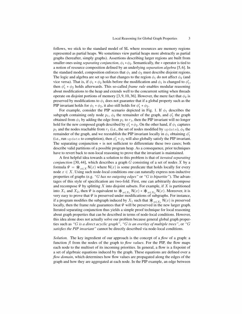
1 method acquire(p: Node, r: Node) {2 if (r.next == null) {3 r.next := p; update(p, -1, r.curr_prio)4 } else {5 p.next := r; update(r, -1, p.curr_prio)6 }7 }8 method update(n: Node, from: Int, to: Int) {9 n.prios := n.prios \ {from}
10 if (to >= 0) n.prios := n.prios ∪ {to}11 from := n.curr_prio12 n.curr_prio := max(n.prios ∪ {n.def_prio})13 to := n.curr_prio;14 if (from != to && n.next != null) {15 update(n.next, from, to)16 }17 }
p13 {2}
r1
0
∅
p2
1
{0}
r20 {1}
p3
2
{1}
r3
{1,2, 2}
0
p41 ∅ p52 ∅
r4 {2, 2}0
p62 ∅
p72 ∅
Fig. 1: Pseudocode of the PIP and a state of the protocol data structure. Round nodesrepresent processes and rectangular nodes resources. Nodes are marked with their defaultpriorities def_prio as well as the aggregate priority multiset prios. A node’s currentpriority curr_prio is underlined and marked in bold blue.
about global graph properties that can be used within off-the-shelf separation logics.We demonstrate our technique using two challenging examples for which no fully localproof existed before, respectively, whose proof required a tailor-made logic.
As a motivating example, we consider an idealized priority inheritance protocol (PIP),a technique used in process scheduling [39]. The purpose of the protocol is to avoidpriority inversion, i.e. a situation where a low-priority process causes a high-priorityprocess to be blocked. The protocol maintains a bipartite graph with nodes representingprocesses and resources. An example graph is shown in Fig. 1. An edge from a processp to a resource r indicates that p is waiting for r to be available whereas an edge inthe other direction means that r is currently held by p. Every node has an associateddefault priority and current; these are natural numbers. The current priority is used forscheduling processes. When a process attempts to acquire a resource currently held byanother process, the graph is updated to avoid priority inversion. For example, whenprocess p1 with current priority 3 attempts to acquire the resource r1 held by processp2 of priority 1, p1’s higher priority is propagated to p2 and, transitively, to any otherprocess that p2 is waiting for (p3 in this case). As a result, all nodes on the created cycle3
will get current priority 3. The protocol maintains the following invariant: the currentpriority of each node is the maximum of its default priority and the current priorities ofall its predecessors. Priority propagation is implemented by the method update shownin Fig 1. The implementation represents graph edges by next pointers and handles bothadding an edge (acquire) and removing one (release - code omitted). To recalculatethe current priority of a node (line 12), each node maintains its default priority def_prioand a multiset prios which contains the priorities of all its immediate predecessors.
Verifying that the PIP maintains its invariant using established separation logic (SL)techniques is challenging. In general, SL assertions describe resources and express thefact that the program has permission to access and manipulate these resources. In what
3 The cycle can be used to detect/handle a deadlock; this is not the concern of this data structure.
Local Reasoning for Global Graph Properties 3
follows, we stick to the standard model of SL where resources are memory regionsrepresented as partial heaps. We sometimes view partial heaps more abstractly as partialgraphs (hereafter, simply graphs). Assertions describing larger regions are built fromsmaller ones using separating conjunction, φ1 ∗φ2. Semantically, the ∗ operator is tied toa notion of resource composition defined by an underlying separation algebra [5, 6]. Inthe standard model, composition enforces that φ1 and φ2 must describe disjoint regions.The logic and algebra are set up so that changes to the region φ1 do not affect φ2 (andvice versa). That is, if φ1 ∗ φ2 holds before the modification and φ1 is changed to φ′1,then φ′1 ∗ φ2 holds afterwards. This so-called frame rule enables modular reasoningabout modifications to the heap and extends well to the concurrent setting when threadsoperate on disjoint portions of memory [3, 9, 10, 36]. However, the mere fact that φ2 ispreserved by modifications to φ1 does not guarantee that if a global property such as thePIP invariant holds for φ1 ∗ φ2, it also still holds for φ′1 ∗ φ2.
For example, consider the PIP scenario depicted in Fig. 1. If φ1 describes thesubgraph containing only node p1, φ2 the remainder of the graph, and φ′1 the graphobtained from φ1 by adding the edge from p1 to r1, then the PIP invariant will no longerhold for the new composed graph described by φ′1 ∗φ2. On the other hand, if φ1 capturesp1 and the nodes reachable from r1 (i.e., the set of nodes modified by update), φ2 theremainder of the graph, and we reestablish the PIP invariant locally in φ1 obtaining φ′1(i.e., run update to completion), then φ′1 ∗φ2 will also globally satisfy the PIP invariant.The separating conjunction ∗ is not sufficient to differentiate these two cases; bothdescribe valid partitions of a possible program heap. As a consequence, prior techniqueshave to revert back to non-local reasoning to prove that the invariant is maintained.
A first helpful idea towards a solution to this problem is that of iterated separatingconjunction [30, 44], which describes a graph G consisting of a set of nodes X by aformula Ψ = ∗x∈X N(x) where N(x) is some predicate that holds locally for everynode x ∈ X . Using such node-local conditions one can naturally express non-inductiveproperties of graphs (e.g. “G has no outgoing edges” or “G is bipartite”). The advan-tages of this style of specification are two-fold. First, one can arbitrarily decomposeand recompose Ψ by splitting X into disjoint subsets. For example, if X is partitionedinto X1 and X2, then Ψ is equivalent to∗x∈X1
N(x) ∗ ∗x∈X2N(x). Moreover, it is
very easy to prove that Ψ is preserved under modifications of subgraphs. For instance,if a program modifies the subgraph induced by X1 such that∗x∈X1
N(x) is preservedlocally, then the frame rule guarantees that Ψ will be preserved in the new larger graph.Iterated separating conjunction thus yields a simple proof technique for local reasoningabout graph properties that can be described in terms of node-local conditions. However,this idea alone does not actually solve our problem because general global graph proper-ties such as “G is a direct acyclic graph”, “G is an overlay of multiple trees”, or “Gsatisfies the PIP invariant” cannot be directly described via node-local conditions.
Solution. The key ingredient of our approach is the concept of a flow of a graph: afunction fl from the nodes of the graph to flow values. For the PIP, the flow mapseach node to the multiset of its incoming priorities. In general, a flow is a fixpoint ofa set of algebraic equations induced by the graph. These equations are defined over aflow domain, which determines how flow values are propagated along the edges of thegraph and how they are aggregated at each node. In the PIP example, an edge between

4 S. Krishna et al.
nodes (n, n′) propagates the multiset containing max(fl(n), n.def_prio) from n ton′. The multisets arriving at n′ are aggregated with multiset union to obtain fl(n′).Flows enable capturing global graph properties in terms of node-local conditions. Forexample, the PIP invariant can be expressed by the following node-local condition:n.curr_prio = max(fl(n), n.def_prio). To enable compositional reasoning aboutsuch properties we need an appropriate separation algebra allowing us to prove locallythat modifications to a subgraph do not affect the flow of the remainder of the graph.
To this end, we make the useful observation that a separation algebra induces anotion of an interface of a resource: we say that two resources a and a′ are equivalentif they compose with the same resources. The interface of a resource a could then bedefined as a’s equivalence class, but more-succinct and simpler representations may bepossible. In the standard model of SL where resources are graphs and composition isdisjoint graph union, the interface of a graph G is the set of all graphs G′ that have thesame domain as G; in this model, a graph’s domain could be defined to be its interface.
The interfaces of resources described by assertions capture the information that isimplicitly communicated when these assertions are conjoined by separating conjunction.As we discussed earlier, in the standard model of SL, this information is too weak toenable local reasoning about global properties of the composed graphs because someadditional information about the subgraphs’ structure other than which nodes theycontain must be communicated. For instance, if the goal is to verify the PIP invariant, theinterfaces must capture information about the multisets of priorities propagated betweenthe subgraphs. We define a separation algebra achieving exactly this: the induced flowinterface of a graph G in this separation algebra captures how values of the flow domainmust enter and leave G such that, when composed with a compatible graph G′, theimposed local conditions on the flow of each node are satisfied in the composite graph.
This is the key to enabling SL-style framing for global graph properties. Using iter-ated separating conjunctions over the new separation algebra, we obtain a compositionalproof technique that yields succinct proofs of programs such as the PIP, whose proofswith existing techniques would involve non-trivial global reasoning steps.
Contributions. In §2, we present mathematical foundations for flow domains, imposingthe minimal requirements on the underlying algebra that allow us to capture a broadrange of data structure invariants and graph properties and reason locally about them in asuitable separation algebra. Building on this theory we develop a general proof techniquefor modular reasoning about global graph properties that can be integrated with existingseparation logics (§3). We further identify general mathematical conditions that can beused when desired to guarantee unique flows, and provide local proof arguments to checkthe preservation of these conditions (§4). We demonstrate the versatility of our approachby presenting local proofs for two challenging examples: the PIP and the concurrentnon-blocking list due to Harris [12].
Flows Redesigned. Our work is inspired by the recent flow framework explored bysome of the authors [22], but was redesigned from the ground up. We revisit the corealgebra behind flow reasoning, and derive a different algebraic foundation by analysingthe minimal requirements for general local reasoning; we call our newly-designedreasoning framework the foundational flow framework. Our new framework makes

Local Reasoning for Global Graph Properties 5
several significant improvements over [22] and eliminates its most stark limitations. Weprovide a detailed technical comparison with [22] and discuss other related work in §5.
2 The Foundational Flow Framework
In this section, we introduce the foundational flow framework, explaining the motivationfor its design with respect to local reasoning principles. We aim for a general techniquefor modularly proving the preservation of recursively-defined invariants over (partial)graphs, with well-defined decomposition and composition operations.
2.1 Preliminaries and Notation
The term (b ? t1 : t2) denotes t1 if condition b holds and t2 otherwise. We write f : A→B for a function from A to B, and f : A ⇀ B for a partial function from A to B. For apartial function f , we write f(x) = ⊥ if f is undefined at x. We use lambda notation(λx. E) to denote a function that maps x to the expression E (typically containing x). Iff is a function from A to B, we write f [x� y] to denote the function from A ∪ {x}defined by f [x� y](z) := (z = x ? y : f(z)). We use {x1� y1, . . . , xn� yn} forpairwise different xi to denote the function ε[x1 � y1] · · · [xn � yn], where ε is thefunction on an empty domain. Given functions f1 : A1 → B and f2 : A2 → B we writef1 ] f2 for the function f : A1 ] A2 → B that maps x ∈ A1 to f1(x) and x ∈ A2 tof2(x) (if A1 and A2 are not disjoint sets, f1 ] f2 is undefined).
We write δn=n′ : M → M for the function defined by δn=n′(m) := m if n = n′
else 0. We also write λ0 := (λm. 0) for the identically zero function, λid := (λm. m)for the identity function, and use e ≡ e′ to denote function equality. For e : M →M andm ∈M we writem.e to denote the function application e(m). We write e◦e′ to denotefunction composition, i.e. (e ◦ e′)(m) = e(e′(m)) for m ∈ M , and use superscriptnotation ep to denote the function composition of e with itself p times.
For multisets S, we use standard set notation when clear from the context. We writeS(x) to denote the number of occurrences of x in S. We write {x1� i1, . . . , xn� in}for the multiset containing i1 occurrences of x1, i2 occurrences of x2, etc.
A partial monoid is a set M , along with a partial binary operation +: M ×M ⇀ M , and a special zero element 0 ∈ M , such that (1) + is associative, i.e.,(m1+m2)+m3 = m1+(m2+m3); and (2) 0 is an identity, i.e., m+0 = 0+m = m.Here, = means either both sides are defined and equal, or both are undefined. Weidentify a partial monoid with its support set M . If + is a total function, then we callM a monoid. Let m1,m2,m3 ∈ M be arbitrary elements of the (partial) monoid inthe following. We call a (partial) monoid M commutative if + is commutative, i.e.,m1 + m2 = m2 + m1. Similarly, a commutative monoid M is cancellative if + iscancellative, i.e., if m1 +m2 = m1 +m3 is defined, then m2 = m3.
A separation algebra [5] is a cancellative, partial, commutative monoid.
2.2 Flows
Recursive properties of graphs naturally depend on non-local information; e.g. we cannotexpress that a graph is acyclic directly as a conjunction of per-node invariants. Our

6 S. Krishna et al.
foundational flow framework defines flow values at each node that capture non-localgraph properties, and enables local specification and reasoning about such properties.Flow values are drawn from a flow domain, an algebraic structure which also specifiesthe operations used to define a flow via recursive computations over the graph. Ourentire theory is parametric with the choice of a flow domain, whose components will beexplained and motivated in the rest of this section.
Definition 1 (Flow Domain). A flow domain (M,+, 0, E) consists of a commutativecancellative (total) monoid (M,+, 0) and a set of edge functions E ⊆M →M .
Example 1. The path-counting flow domain is (N,+, 0, {λid, λ0}), consisting of themonoid of natural numbers under addition and the set of edge functions containing onlythe identity function and the zero function. This can be used to define a flow where thevalues at each node represent the number of paths to this node from a distinguished noden. Path-counting provides enough information to express locally per node that e.g. (a)all nodes are reachable from n (all path counts are non-zero), or (b) that the graph formsa tree rooted at n (all path counts are exactly 1).
Example 2. We use (NN,∪, ∅, {λ0} ∪ {(λm. {max(m ∪ {p})}) | p∈N}) as flow do-main for the PIP example (Figure 1). This consists of the monoid of multisets of naturalnumbers under multiset union and two kinds of edge functions: λ0 and functions map-ping a multiset m to the singleton multiset containing the maximum value between mand a fixed value p (used to represent a node’s default priority). This can define a flowwhich locally captures the appropriate current node priorities as the graph is modified.
Further definitions in this section assume a fixed flow domain (M,+, 0, E) and a(potentially infinite) set of nodes N. For this section, we abstract heaps using directedpartial graphs; integration of our graph reasoning with direct proofs over program heapsis explained in §3.
Definition 2 (Graph). A (partial) graph G = (N, e) consists of a finite set of nodesN ⊆ N and a mapping from pairs of nodes to edge functions e : N ×N→ E.
Flow Values and Flows. Flow values (taken from M ; the first element of a flow domain)are used to capture sufficient information to express desired non-local properties of agraph. In Example 1, flow values are non-negative integers; for the PIP (Example 2)we instead use multisets of integers, representing relevant non-local information: thepriorities of nodes currently referencing a given node in the graph. Given such flow values,a node’s correct priority can be defined locally per node in the graph. This definitionrequires only the maximum value of these multisets, but as we will see shortly thesemultisets enable local recomputation of a correct priority when the graph is changed.
For a graph G = (N, e) we express properties of G in terms of node-local conditionsthat may depend on the nodes’ flow. A flow is a function fl : N →M assigning everynode a flow value and must be some fixpoint of the following flow equation:
∀n ∈ N. fl(n) = in(n) +∑n′∈N
fl(n′) . e(n′, n) (FlowEqn)

Local Reasoning for Global Graph Properties 7
Intuitively, one can think of the flow as being obtained by a fold computation over thegraph:4 the inflow in : N → M defines an initial flow at each node. This initial flowis then updated recursively for each node n: the current flow value at its predecessornodes n′ is transferred to n via edge functions e(n′, n) : M →M . These flow values areaggregated using the summation operation + of the flow domain to obtain an updatedflow of n; a flow for the graph is some fixpoint satisfying this equation at all nodes. 5
Definition 3 (Flow Graph). A flow graphH = (N, e,fl) is a graph (N, e) and functionfl : N →M such that there exists an inflow in : N →M satisfying FlowEqn(in, e,fl).
We let dom(H) = N , and sometimes identify H and dom(H) to ease notationalburden. For n ∈ H we write Hn for the singleton flow subgraph of H induced by n.
Edge Functions. In any flow graph, the flow value assigned to a node n by a flowis propagated to its neighbours n′ (and transitively) according to the edge functione(n, n′) labelling the edge (n, n′). The edge function maps the flow value at the sourcenode n to one propagated on this edge to the target node n′. Note that we require sucha labelling for all pairs consisting of a source node n inside the graph and a targetnode n′ ∈ N (i.e., possibly outside the graph). The 0 flow value (the third elementof our flow domains) is used to represent no flow; the corresponding (constant) zerofunction λ0 = (λm. 0) is used as edge function to model the absence of an edge in thegraph. A set of edge functions E from which this labelling is chosen can, other thanthe requirement λ0 ∈ E, be chosen as desired. As we will see in §4.4, restrictions toparticular sets of edge functions E can be exploited to further strengthen our overalltechnique. Edge functions can depend on the local state of the source node (as in thefollowing example); dependencies from elsewhere in the graph must be represented bythe node’s flow.
Example 3. Consider the graph in Figure 1 and the flow domain as in Example 2. Wechoose the edge functions to be λ0 where no edge exists in the PIP structure, and other-wise (λm. {max(m ∪ {d})}) where d is the default priority of the source of the edge.For example, in Figure 1, e(r3, p2) = λ0 and e(r3, p1) = (λm. {max(m ∪ {0})}).Since the flow value at r3 is {1, 2, 2}, the edge (r3, p1) propagates the value {2} to p1,correctly representing the current priority of r3.
Flow Aggregation and Inflows. The flow value at a node is defined by those propagatedto it from each node in a graph via edge functions, along with an additional inflow valueexplained here. Since multiple non-zero flow values can be propagated to a node, werequire an aggregation of these values via a binary + operator on flow values : the secondelement of our flow domains. The edges from which the aggregated values originateare unordered. Thus, we require + to be commutative and associative, making thisaggregation order-independent. The 0 flow value must act as a unit for +. For example,in the path-counting flow domain + means addition on natural numbers, while for themultisets employed for the PIP it means multiset union.
4 We note that flows are not generally defined in this manner as we consider any fixpoint of theflow equation to be a flow. Nonetheless, the analogy helps to build an initial intuition.
5 We discuss questions regarding the existence and uniqueness of such fixpoints in §4.

8 S. Krishna et al.
Each node in a flow graph has an inflow, modelling contributions to its flow valuewhich do not come from inside the graph. Inflows play two important roles: first, sinceour graphs are partial, they model contributions from nodes outside of the graph. Second,inflow can be artificially added as a means of specialising the computation of flow valuesto characterise specific graph properties. For example, in the path-counting domain, wegive an inflow of 1 to the node from which we are counting paths, and 0 to all others.
Example 4. Let the edges in the graph in Figure 1 be labelled as described in Example 3.If the inflow function in assigns the empty multiset to every node n and we let fl(n) bethe multiset labelling every node in the figure, then FlowEqn(in, e,fl) holds.
The flow equation (FlowEqn) defines the flow of a node n to be the aggregation offlow values coming from other nodes n′ inside the graph (as given by the respective edgefunction e(n′, n)) as well as the inflow in(n). Preserving solutions to this equation acrossupdates to the graph structure is a fundamental goal of our technique. The followinglemma (which relies on the fact that + is required to be cancellative) states that anycorrect flow values uniquely determine appropriate inflow values:
Lemma 1. Given a flow graph (N, e,fl), there exists a unique inflow in such thatFlowEqn(in, e,fl).
We now turn to how solutions of the flow equation can be preserved or appropriatelyupdated under changes to the underlying graph.
Graph Updates and Cancellativity. Given a flow graph with known flow and inflowvalues, suppose we remove an edge from n1 to n2 (replacing the edge function withλ0). For the same inflow, such an update will potentially affect the flow at n2 and nodesto which n2 (transitively) propagates flow. Starting from the simple case that n2 hasno outgoing edges, we need to recompute a suitable flow at n2. Knowing the old flowvalue (say, m) and the contribution m′ = fl(n1) . e(n1, n2) previously provided alongthe removed edge, we know that the correct new flow value is some m′′ such thatm′ +m′′ = m. This constraint has a unique solution (and thus, we can unambiguouslyrecompute a new flow value) exactly when the aggregation + is cancellative; we thereforemake cancellativity a requirement on the + of any flow domain.
Cancellativity intuitively enforces that the flow domain carries enough informationto enable adaptation to local updates (in particular, removal of edges6). Returning to thePIP example, cancellativity requires us to carry multisets as flow values rather than onlythe maximum priority value: + cannot be the maximum operation, as this would not becancellative. The resulting multisets (like the prio fields in the actual code) provide theinformation necessary to recompute corrected priority values locally.
For example, in the PIP graph shown in Figure 1, removing the edge from p6 tor4would not affect the current priority of r4 whereas if p7 had current priority 1 insteadof 2, then the current priority of r4 would have to decrease. In either case, recomputingthe flow value for r4 is simply a matter of subtraction (removing {2} from the multiset atr4); cancellativity guarantees that our flow domains will always provide the information
6 As we will show in §2.3, an analogous problem for composition of flow graphs is also directlysolved by this choice to force aggregation to be cancellative.
Local Reasoning for Global Graph Properties 9
needed for this recomputation. Without this property, the recomputation of a flow valuefor the target node n2 would, in general, entail recomputing the incoming flow valuesfrom all remaining edges from scratch. Cancellativity is also crucial for Lemma 1 above,forcing uniqueness of inflows, given known flow values in a flow graph. This allows usto define natural but powerful notions of flow graph decomposition and recomposition.
2.3 Flow Graph Composition and Abstraction
Building towards the core of our reasoning technique, we now turn to the questionof decomposition and recomposition of flow graphs. Two flow graphs with disjointdomains always compose to a graph, but this will be a flow graph only if their flows arechosen consistently to admit a solution to the resulting flow equation (i.e. the flow graphcomposition operator � defined below is partial).
Definition 4 (Flow Graph Algebra). The flow graph algebra (FG,�, H∅) for the flowdomain (M,+, 0, E) is defined by
FG := {(N, e,fl) | (N, e,fl) is a flow graph} , H∅ := (∅, e∅,fl∅),
(N1, e1,fl1)� (N2, e2,fl2) :=
{(N1 ]N2, e1 ] e2,fl1 ] fl2) if in FG
⊥ otherwise,
where e∅ and fl∅ are the edge functions and flow on the empty set of nodes N = ∅.
Intuitively, two flow graphs compose to a flow graph if their contributions to eachothers’ flow (along edges from one to the other) are reflected in the corresponding inflowof the other graph. For example, consider the subgraph from Figure 1 consisting ofthe single node p7 (with 0 inflow). This will compose with the remainder of the graphdepicted only if this remainder subgraph has an inflow which, at node r4, includes atleast the multiset {2}, reflecting the propagated value from p7.
We use this intuition to extract an abstraction of flow graphs which we call flowinterfaces. Given a flow (sub)graph, its flow interface consists of the node-wise inflowand outflow (the flow contributions its nodes make to all nodes outside of the graph,defined below). It is thus an abstraction that hides the flow values and edges that arewholly inside the flow graph. Flow graphs that have the same flow interface “look thesame” to the external graph, as the same values are propagated inwards and outwards.
Definition 5 (Flow Interface). For a given flow domain M , a flow interface is a pairI = (in, out) where in : N →M and out : N \N →M for some N ⊆ N.
We write I.in, I.out for the two components of the interface I = (in, out). We willagain sometimes identify I and dom(I.in) to ease notational burden.
Given a flow graph H ∈ FG, we can compute its interface as follows. Recall thatLemma 1 implies that any flow graph has a unique inflow. Thus, we can define an inflowfunction that maps each flow graph H = (N, e,fl) to the unique inflow inf(H) : H →M such that FlowEqn(inf(H), e,fl). Dually, we define the outflow of H as the functionoutf(H) : N \ N → M defined by outf(H)(n) :=
∑n′∈N fl(n′) . e(n′, n). The flow
interface of H , written int(H), is the pair (inf(H), outf(H)) consisting of its inflow

10 S. Krishna et al.
and its outflow. Returning to the previous example, if H is the singleton subgraphconsisting of node p7 from Figure 1 with flow and edges as depicted, then int(H) =(λn. ∅, λn. (n=r4 ? {2} : ∅)).
This abstraction, while simple, turns out to be powerful enough to build a separationalgebra over our flow graphs, allowing them to be decomposed, locally modified andrecomposed in ways yielding all the local reasoning benefits of separation logics. Inparticular, for graph operations within a subgraph with a certain interface, we need toprove: (a) that the modified subgraph is still a flow graph (by checking that the flowequation still has a solution locally in the subgraph) and (b) that it satisfies the sameinterface (in other words, the effect of the modification on the flow is contained withinthe subgraph); the meta-level results for our technique then justify that we can recomposethe modified subgraph with any graph that the original could be composed with.
We define the corresponding flow interface algebra as follows:
Definition 6 (Flow Interface Algebra). For a given flow domain M , the flow interfacealgebra over M is defined to be (FI,⊕, I∅), where:
FI := {I | I is a flow interface} , I∅ := int(H∅),
I1 ⊕ I2 :=
I I1 ∩ I2 = ∅
∧ ∀i 6= j ∈ {1, 2} , n ∈ Ii. Ii.in(n) = I.in(n) + Ij .out(n)
∧ ∀n 6∈ I. I.out(n) = I1.out(n) + I2.out(n)
⊥ otherwise.
Flow interface composition is well-defined because of cancellativity of the underlyingflow domain (it is also, exactly as flow graph composition, partial). We next show thekey result for this abstraction: the ability for two flow graphs to compose depends onlyon their interfaces; flow interfaces implicitly define a congruence relation on flow graphs.
Lemma 2. int(H1) = I1 ∧ int(H2) = I2 ⇒ int(H1 �H2) = I1 ⊕ I2.
Crucially, the following result shows that we can use our flow interfaces as anabstraction directly compatible with existing separation logics.
Theorem 1. The flow interface algebra (FI,⊕, I∅) is a separation algebra.
This result forms the core of our reasoning technique; it enables us to make modifi-cations within a chosen subgraph and, by proving preservation of its interface, know thatthe result composes with any context exactly as the original did. Flow interfaces cap-ture precisely the information relevant about a flow graph, with respect to compositionwith other flow graphs. In Appendix B of the accompanying technical report (hereafter,TR) [23] we provide additional examples of flow domains that demonstrate the range ofdata structures and graph properties that can be expressed using flows, including a notionof universal flow that in a sense provides a completeness result for the expressivity ofthe framework. We now turn to constructing proofs atop these new reasoning principles.
Local Reasoning for Global Graph Properties 11
3 Proof Technique
This section shows how to integrate flow reasoning into a standard separation logic,using the priority inheritance protocol (PIP) algorithm to illustrate our proof techniques.
Since flow graphs and flow interfaces form separation algebras, it is possible inprinciple to define a separation logic (SL) using these notions as a custom semanticmodel (indeed, this is the proof approach taken in [22]). By contrast, we integrate flowinterfaces with a standard separation logic without modifying its semantics. This hasthe important technical advantage that our proof technique can be naturally integratedwith existing separation logics and verification tools supporting SL-style reasoning. Weconsider a standard sequential SL in this section, but our technique can also be directlyintegrated with a concurrent SL such as RGSep (as we show in §4.5) or frameworks suchas Iris [18] supporting (ghost) resources ranging over user-defined separation algebras.
3.1 Encoding Flow-based Proofs in SL
Proofs using our flow framework can employ a combination of specifications enforcedat the node level and in terms of the flow graphs and interfaces corresponding to largerheap regions such as entire data structures (henceforth, composite graphs and compositeinterfaces). At the node level, we write invariants that every node is intended to satisfy,typically relating the node’s flow value to its local state (fields). For example, in the PIP,we use node-local invariants to express that a node’s current priority is the maximum ofthe node’s default priority and those in its current flow value. We typically express suchspecifications in terms of singleton (flow) graphs, and their singleton interfaces.
Specification in terms of composite interfaces has several important purposes. Oneis to define custom inflows: e.g. in the path-counting flow domain, specifying that theinflow of a composite interface is 1 at some designated node r and 0 elsewhere enforcesin any underlying flow graph that each node n’s flow value will be the number of pathsfrom r to n.7 Composite interfaces can also be used to express that, in two states ofexecution, a portion of the heap “looks the same” with respect to composition (it has thesame interface, and so can be composed with the same flow graphs), or to capture byhow much there is an observable difference in inflow or outflow; we employ this idea inthe PIP proof below.
We now define an assertion syntax convenient for capturing both node-level andcomposite-level constraints, defined within an SL-style proof system. We assume an intu-itionistic, garbage-collected SL [6] with standard syntax and semantics:8 see Appendix Aof the TR [23] for more details.
Node Predicates. The basic building block of our flow-based specifications is a nodepredicate N(x,H), representing ownership of the fields of a single node x, as well as
7 Note that the analogous property cannot be captured at the node level; when consideringsingleton interfaces per node in a tree rooted at r, every singleton interface has an inflow of 1.
8 As P ∗ φ ≡ P ∧ φ for pure formulas P in garbage-collected SLs, we use ∗ instead of ∧throughout this paper.

12 S. Krishna et al.
capturing its corresponding singleton flow graph H:
N(x,H) := ∃fs,fl . x 7→ fs ∗H = ({x} , (λy. edge(x, fs, y)), fl) ∗ γ(x, fs,fl(x))
N is implicitly parameterised by fs, edge and γ; these are explained next and are typicallyfixed across any given flow-based proof. The N predicate expresses that we have a heapcell at location x containing fields fs (a list of field-name/value mappings).9 It alsosays that H is a singleton flow graph with domain {x} with some flow fl , whose edgefunctions are defined by a user-defined abstraction function edge(x, fs, y); this functionallows us to define edges in terms of x’s field values. Finally, the node, its fields, andits flow in this flow graph satisfy the custom predicate γ, used to encode node-localproperties such as constraints in terms of the flow values of nodes.
Graph Predicates. The analogous predicate for composite graphs is Gr. It carries owner-ship to the nodes making up a potentially unbounded graph, using iterated separatingconjunction over a set of nodes X as mentioned in §1:
Gr(X,H) := ∃H.∗x∈X
N(x,H(x)) ∗ H =⊙x∈XH(x)
Gr is also implicitly parameterised by fs, edge and γ. The existentially-quantifiedH isa logical variable representing a function from nodes in X to corresponding singletonflow graphs. Gr(X,H) describes a set of nodes X , such that each x ∈ X is an N (inparticular, it satisfies γ), whose singleton flow graphs compose back to H . As well ascarrying ownership of the underlying heap locations, Gr’s definition allows us to connecta node-level view of the region X (eachH(x)) with a composite-level view defined byH , on which we can impose appropriate graph-level properties such as constraints onthe region’s inflow.
Lifting to Interfaces. Flow based proofs can often be expressed more elegantly andabstractly using predicates in terms of node and composite-level interfaces rather thanflow graphs. To this end, we overload both our node and graph predicates with analogueswhose second parameter is a flow interface, defined as follows:
N(x, I) := ∃H. N(x,H) ∗ I = int(H)Gr(X, I) := ∃H. Gr(x,H) ∗ I = int(H)
We will use these versions in the PIP proof below; interfaces capture all relevant proper-ties for decomposition and composition of these flow graphs.
Flow Lemmas. We first illustrate our N and Gr predicates (which capture SL ownershipof heap regions and abstract these with flow interfaces) by identifying a number oflemmas which are generically useful in flow-based proofs. Reasoning at the level of flowinterfaces is entirely in the pure world (mathematics independent of heap-ownership and
9 For simplicity, we assume that all fields of a flow graph node are to be handled by our flow-based technique, and that their ownership (via 7→ points-to predicates) is always carried aroundtogether; lifting these restrictions would be straightforward.
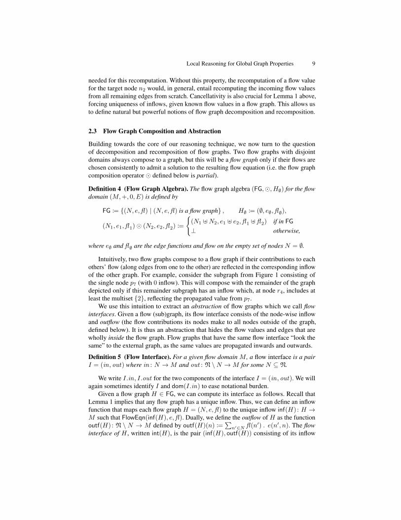
Local Reasoning for Global Graph Properties 13
Gr(X1 ]X2, H) |= ∃H1, H2. Gr(X1, H1) ∗ Gr(X2, H2)
∗H1 �H2 = H (DECOMP)
Gr(X1, H1) ∗ Gr(X2, H2) ∗H1 �H2 6= ⊥ |= Gr(X1 ]X2, H1 �H2) (COMP)
N(x,H) ≡ Gr({x} , H) (SING)
emp |= Gr(∅, H∅) (GREMP)
Gr(X1, H′1) ∗ Gr(X2, H2) ∗H = H1 �H2 |= Gr(X1 ]X2, H
′1 �H2) (REPL)
∗ int(H1) = int(H ′1) ∗ int(H) = int(H ′
1 �H2)
Fig. 2: Some useful lemmas for proving entailments between flow-based specifications.
resources) with respect to the underlying SL reasoning; these lemmas are consequencesof our predicate definitions and the foundational flow framework definitions themselves.
Examples of these lemmas are shown in Figure 2. (DECOMP) shows that we canalways decompose a valid flow graph into subgraphs which are themselves flow graphs.Recomposition (COMP) is possible only if the subgraphs compose. These rules, as wellas (SING), and (GREMP) follow directly from the definition of Gr and standard SL prop-erties of iterated separating conjunction. The final rule (REPL) is a direct consequence ofrules (COMP), (DECOMP) and the congruence relation on flow graphs induced by theirinterfaces (cf. Lemma 2). Conceptually, it expresses that after decomposing any flowgraph into two parts H1 and H2, we can replace H1 with a new flow graph H ′1 with thesame interface; when recomposing, the overall graph will be a flow graph with the sameoverall interface.
Note the connection between rules (COMP)/(DECOMP) and the algebraic laws ofstandard inductive predicates such as ls describing a segment of a linked list [2]. Forinstance by combining the definition of Gr with these rules and (SING) we can prove thefollowing graph analogue of the rule to separate a list into the head node and the tail:
Gr(X ] {y} , H) ≡ ∃Hy, H′.N(y,Hy) ∗ Gr(X,H ′) ∗H = Hy �H ′ ((UN)FOLD)
However, crucially (and unlike when using general inductive predicates [32]), this ruleis symmetrical for any node x in X; it works analogously for any desired order ofdecomposition of the graph, and for any data structure specified using flows.
When working with our overloaded N and Gr predicates, similar steps to thosedescribed by the above lemmas are useful. Given these overloaded predicates, we simplyapply the lemmas above to the existentially quantified flow-graphs in their definitions andthen lift the consequence of the lemma back to the interface level using the congruencebetween our flow graph and interface composition notions (Lemma 2).
3.2 Proof of the PIP
We now have all the tools necessary to verify the priority inheritance protocol (PIP).Figure 3 gives the full algorithm with flow-based specifications; we also include someintermediate assertions to illustrate the reasoning steps for the acquire method, which
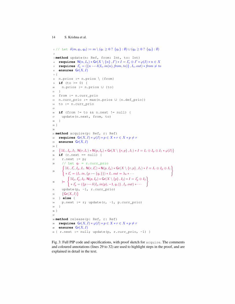
14 S. Krishna et al.
1 // Let δ(m, q1, q2) := m \ (q1 ≥ 0 ? {q1} : ∅) ∪ (q2 ≥ 0 ? {q2} : ∅)2
3 method update(n: Ref, from: Int, to: Int)4 requires N(n, In) ∗ Gr(X \ {n} , I ′) ∗ I = I ′n ⊕ I ′ ∗ ϕ(I) ∗ n ∈ X5 requires I ′n = ({n� δ(In.in(n), from, to)} , In.out) ∗ from 6= to6 ensures Gr(X, I)7 {8 n.prios := n.prios \ {from}9 if (to >= 0) {
10 n.prios := n.prios ∪ {to}11 }12 from := n.curr_prio13 n.curr_prio := max(n.prios ∪ {n.def_prio})14 to := n.curr_prio15
16 if (from != to && n.next != null) {17 update(n.next, from, to)18 }19 }20
21 method acquire(p: Ref, r: Ref)22 requires Gr(X, I) ∗ ϕ(I) ∗ p ∈ X ∗ r ∈ X ∗ p 6= r23 ensures Gr(X, I)24 {
25{∃Ir, Ip, I1. N(r, Ir) ∗ N(p, Ip) ∗ Gr(X \ {r, p} , I1) ∗ I = Ir ⊕ Ip ⊕ I1 ∗ ϕ(I)
}26 if (r.next == null) {27 r.next := p;28 // Let qr = r.curr_prio
29
{∃Ir, I ′r, Ip, I1. N(r, I ′r) ∗ N(p, Ip) ∗ Gr(X \ {r, p} , I1) ∗ I = Ir ⊕ Ip ⊕ I1∗ I ′r = (Ir.in, {p� {qr}}) ∗ Ir.out = λ0 ∗ · · ·
}
30 |=
{∃Ip, I ′p, I2. N(p, Ip) ∗ Gr(X \ {p} , I2) ∗ I = I ′p ⊕ I2∗ I ′p = ({p� δ(Ip.in(p),−1, qr)} , Ip.out) ∗ · · ·
}31 update(p, -1, r.curr_prio)
32{Gr(X, I)
}33 } else {34 p.next := r; update(r, -1, p.curr_prio)35 }36 }37
38 method release(p: Ref, r: Ref)39 requires Gr(X, I) ∗ ϕ(I) ∗ p ∈ X ∗ r ∈ X ∗ p 6= r40 ensures Gr(X, I)41 { r.next := null; update(p, r.curr_prio, -1) }
Fig. 3: Full PIP code and specifications, with proof sketch for acquire. The commentsand coloured annotations (lines 29 to 32) are used to highlight steps in the proof, and areexplained in detail in the text.

Local Reasoning for Global Graph Properties 15
we explain in more detail below. 10 We instantiate our framework in order to capture thePIP invariants as follows:
fs :={next : y, curr_prio : q, def_prio : q0, prios : Q
}edge(x, fs, z) :=
{(λm. max(m ∪ {q0})) if z = y 6= null
λ0 otherwise
γ(x, fs,m) := q0 ≥ 0 ∗ (∀q′ ∈ Q. q′ ≥ 0) ∗ m = Q ∗ q ={max(Q ∪ {q0})
}ϕ(I) := I = (λ0, λ0)
Each node has the four fields listed in fs . fs also defines variables such as y to denotefield values that are used in the definitions of edge and γ; these variables are bound to theheap by N. edge abstracts the heap into a flow graph by letting each node have an edgeto its next successor labelled by a function that passes to it the maximum incomingpriority or the node’s default priority: whichever is larger. With this definition, one cansee that the flow of every node will be the multiset containing exactly the priorities ofits predecessors. The node-local invariant γ says that all priorities are non-negative, theflow m of each node is stored in the prios field, and its current priority is the maximumof its default and incoming priorities. Finally, the constraint ϕ on the global interfaceexpresses that the graph is closed – it has no inflow or outflow.
Flows Specifications for the PIP. Our specifications of acquire and release guaranteethat if we start with a valid flow graph (closed, according to ϕ), we are guaranteed toreturn a valid flow graph with the same interface (i.e. the graph remains closed). Forclarity of the exposition, we focus here on how we prove that being a flow graph thatsatisfies the PIP invariant is preserved (as is the composite flow graph’s interface).Extending this specification to one which proves, e.g., that acquire adds the expectededge is straightforward (see Appendix C of the TR [23]). 11
The specification for update is somewhat subtle, and exploits the full flexibilityof flow interfaces as a specification medium. The preconditions of update describe anupdate to the graph which is not yet completed. There are three complementary aspectsto this specification. Firstly, (as for acquire and release), node-local invariants (γ)hold for all nodes in the graph (enforced via N and Gr predicates). Secondly, we employflow interfaces to express a decomposition of the original top-level interface I intocompatible (primed) sub-interfaces. The key to understanding this specification is thatI ′n is in some sense a fake interface; it does not abstract the current state of the heap noden. Instead, I ′n expresses the way in which the node n’s current inflow hasn’t yet beenaccounted for in the heap: that if n could adjust its inflow according to the propagatedpriority change without changing its outflow, then it would compose back with the rest ofthe graph, and restore the graph’s overall interface. The shorthand δ defines the requiredchange to n’s inflow.
In general (except when n’s next field is null, or n’s flow value is unchanged), itis not even possible for n’s fields to be updated to satisfy I ′n; by updating n’s inflow,10 In specifications, we implicitly quantify at the top level over free variables such as I . λ0 denotes
an identically zero function on an unconstrained domain.11 We also omit acquire’s precondition that p.next == null for brevity.

16 S. Krishna et al.
we will necessarily update its outflow. However, we can then construct a corresponding“fake” interface for the next node in the graph, reflecting the update yet to be accountedfor, and establishing the precondition for the recursive call to update.
The third specification aspect is the connection between heap-level nodes and in-terfaces. The N(n, In) predicate connects n with a different interface; In is the actualcurrent abstraction of n’s state. Conceptually, the key property which is broken at thispoint is this connection between the interface-level specification and the heap at node n,reflected by the decomposition in the specification between X \ {n} and {n}.
We note that the same specification ideas and proof style can be easily adapted toother data structure implementations with an update-notify style, including well-knowndesigns such as Subject-Observer patterns, or the Composite pattern [27].
Proof Outline. To illustrate the application of flows reasoning to our PIP specificationideas more clearly, we examine in detail the first if-branch in the proof of acquire. Ourintermediate proof steps are shown as purple annotations surrounded by braces. The firststep, as shown in the first line inside the method body, is to apply ((UN)FOLD) twice (onthe flow graphs represented by these predicates) and peel off N predicates for each of rand p. The update to r’s next field (line 27) causes the correct singleton interface of r tochange to I ′r: its outflow (previously none, since the next field was null) now propagatesflow to p. We summarise this state in the assertion on line 29 (we omit e.g. repetitionof properties from the function’s precondition, focusing on the flow-related steps ofthe argument). We now rewrite this state; using the definition of interface composition(Definition 6) we deduce that although I ′r and Ip do not compose (since the former hasoutflow that the latter does not account for as inflow), the alternative “fake” interfaceI ′p for p (which artificially accounts for the missing inflow) would do so (cf. line 30).Essentially, we show Ir ⊕ Ip = I ′r ⊕ I ′p, that the interface of {r, p} would be unchangedif p could somehow have interface I ′p. Now by setting I2 = I ′r ⊕ I1 and using algebraicproperties of interfaces, we assemble the precondition expected by update. After thecall, update’s postcondition gives us the desired postcondition.
We focused here on the details of acquire’s proof, but very similar manipulationsare required for reasoning about the recursive call in update’s implementation.12 Themain difference there is that if the if-condition wrapping the recursive call is false theneither the last-modified node has no successor (and so there is no outstanding inflowchange needed), or we have from= to which implies that the “fake” interface is actuallythe same as the currently correct one.
Despite the property proved for the PIP example being a rather delicate recursive in-variant over the (potentially cyclic) graph, the power of our framework enables extremelysuccinct specifications for the example, and proofs which require the application of rela-tively few generic lemmas. The integration with standard separation logic reasoning, andthe complementary separation algebras provided by flow interfaces allow decompositionand recomposition to be simple proof steps. For this proof, we integrated with standardsequential separation logic, but in the next section we will show that compatibility withconcurrent SL techniques is similarly straightforward.
12 We provide further proof outlines in Appendix C of the TR [23].

Local Reasoning for Global Graph Properties 17
mh −∞ 3 5 9 10 12 ∞
fh 2 6 1 7 ft
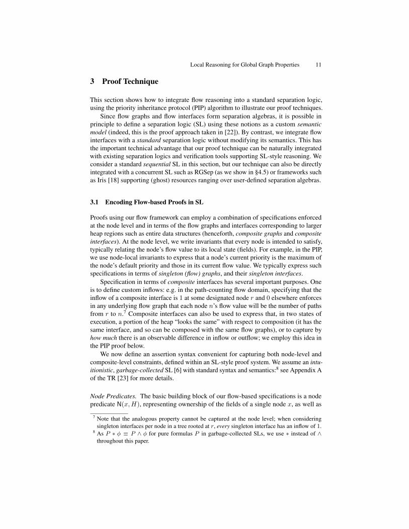
Fig. 4: A potential state of the Harris list with explicit memory management. fnextpointers are shown with dashed edges, marked nodes are shaded gray, and null pointersare omitted for clarity.
4 Advanced Flow Reasoning and the Harris List
This section introduces some advanced foundational flow framework theory and demon-strates its use in the proof of the Harris list. We note that [22] presented a proof of thisdata structure in the original flow framework. The proof given here shows that the newframework eliminates the need for the customized concurrent separation logic definedin [22]. We start with a recap of Harris’ algorithm adapted from [22].
4.1 The Harris List Algorithm
The power of flow-based reasoning is exhibited in the proof of overlaid data structuressuch as the Harris list, a concurrent non-blocking linked list algorithm [12]. This algo-rithm implements a set data structure as a sorted list, and uses atomic compare-and-swap(CAS) operations to allow a high degree of parallelism. As with the sequential linkedlist, Harris’ algorithm inserts a new key k into the list by finding nodes k1, k2 such thatk1 < k < k2, setting k to point to k2, and using a CAS to change k1 to point to k onlyif it was still pointing to k2. However, a similar approach fails for the delete operation.If we had consecutive nodes k1, k2, k3 and we wanted to delete k2 from the list (say bysetting k1 to point to k3), there is no way to ensure with one CAS that k2 and k3 are alsostill adjacent (another thread could have inserted/deleted in between them).
Harris’ solution is a two step deletion: first atomically mark k2 as deleted (by settinga mark bit on its successor field) and then later remove it from the list using a singleCAS. After a node is marked, no thread can insert or delete to its right, hence a threadthat wanted to insert k′ to the right of k2 would first remove k2 from the list and theninsert k′ as the successor of k1.
In a non-garbage-collected environment, unlinked nodes cannot be immediately freedas suspended threads might continue to hold a reference to them. A common solutionis to maintain a second “free list” to which marked nodes are added before they areunlinked from the main list (this is the so-called drain technique). These nodes are thenlabelled with a timestamp, which is used by a maintenance thread to free them when it issafe to do so. This leads to the kind of data structure shown in Figure 4, where each nodehas two pointer fields: a next field for the main list and an fnext field for the free list(the list from fh to ft via dashed edges). Threads that have been suspended while holding

18 S. Krishna et al.
1
?
?
1
(a)
1
x
x
1
(b)
1 n1 1n2
1n3 1 n4
1
n5
1
1 n1 1n2
1n3 1 n4
1
n5
1
(c)
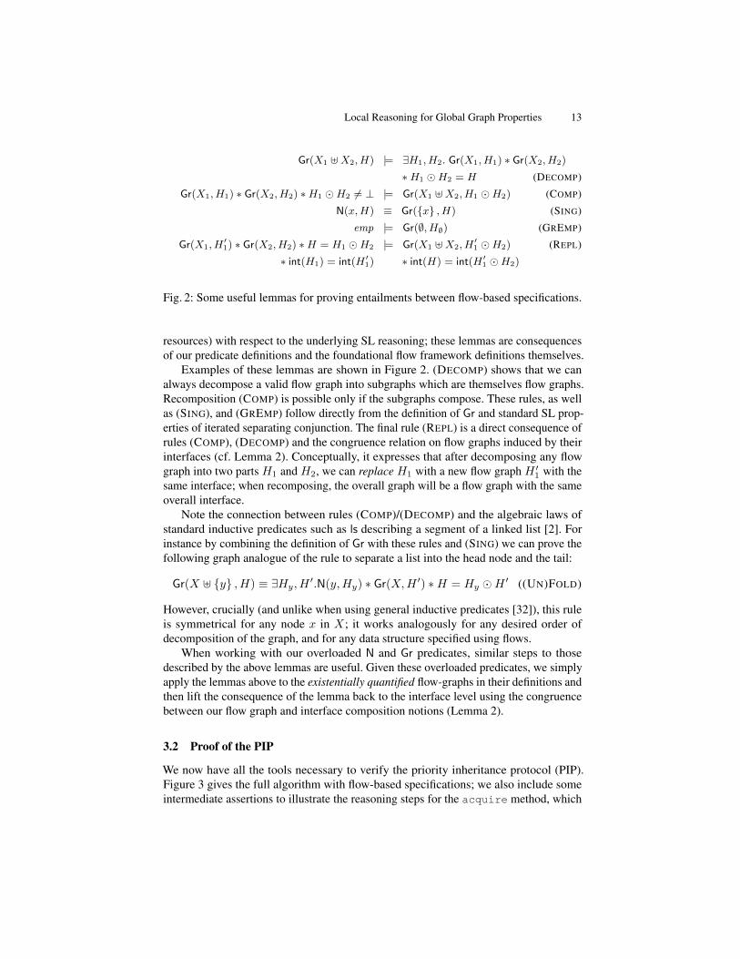
Fig. 5: Examples of graphs that motivate effective acyclicity. All graphs use the path-counting flow domain, the flow is displayed inside each node, and the inflow is displayedas curved arrows to the top-left of nodes. (a) shows a graph and inflow that has nosolution to (FlowEqn); (b) has many solutions. (c) shows a modification that preservesthe interface of the modified nodes, yet goes from a graph that has a unique flow to onethat has many solutions to (FlowEqn).
a reference to a node that was added to the free list can simply continue traversing thenext pointers to find their way back to the unmarked nodes of the main list.
Even for seemingly simple properties such as that the Harris list is memory safe andnot leaking memory, the proof will rely on the following non-trivial invariants:
(a) The data structure consists of two (potentially overlapping) lists: a list on next
edges beginning at mh and one on fnext edges beginning at fh .(b) The two lists are null terminated and next edges from nodes in the free list point to
nodes in the free list or main list.(c) All nodes in the free list are marked.(d) ft is an element in the free list (due to concurrency, it’s not always the tail).
Challenges. To prove that Harris’ algorithm maintains the invariants listed above wemust tackle a number of challenges. First, we must construct flow domains that allow usto describe overlaid data structures, such as the overlapping main and free lists (§4.2).Second, the flow-based proofs we have seen so far work by showing that the interface ofsome modified region is unchanged. However, if we consider a program that allocatesand inserts a new node into a data structure (like the insert method of Harris), then theinterface cannot be the same since the domain has changed (it has increased by thenewly allocated node). We must thus have a means to reason about preservation of flowsby modifications that allocate new nodes (§4.3). The third issue is that in some flowdomains, there exist graphs G and inflows in for which no solutions to the flow equation(FlowEqn) exist. For instance, consider the path-counting flow domain and the graphin Figure 5(a). Since we would need to use the path-counting flow in the proof of theHarris list to encode its structural invariants, this presents a challenge (§4.4).
We will next see how to overcome these three challenges in turn, and then applythose solution to the proof of the Harris list in §4.5.

Local Reasoning for Global Graph Properties 19
4.2 Product Flows for Reasoning about Overlays
An important fact about flows is that any flow of a graph over a product of two flowdomains is the product of the flows on each flow domain component.
Lemma 3. Given two flow domains (M1,+1, 01, E1) and (M2,+2, 02, E2), the productdomain (M1 ×M2,+, (01, 02), E) is a flow domain, where + and E are the pointwiseliftings of (+1,+2) and (E1, E2), respectively, to the domain M1 ×M2.
This lemma greatly simplifies reasoning about overlaid graph structures; we will usethe product of two path-counting flows to describe a structure consisting of two overlaidlists that make up the Harris list.
4.3 Contextual Extensions and the Replacement Theorem
In general, when modifying a flow graph H to another flow graph H ′, requiring that H ′
satisfies precisely the same interface int(H) can be too strong a condition as it does notpermit allocating new nodes. Instead, we want to allow int(H ′) to differ from int(H)in that the new interface could have a larger domain, as long as the edges from the newnodes do not change the outflow of the modified region.
Definition 7. An interface I = (in, out) is contextually extended by I ′ = (in ′, out ′),written I - I ′, if and only if the following conditions all hold:
(1) dom(in) ⊆ dom(in ′),(2) ∀n ∈ dom(in). in(n) = in ′(n), and(3) ∀n′ 6∈ dom(in ′). out(n′) = out ′(n′).
The following theorem states that contextual extension preserves composability andis itself preserved under interface composition.
Theorem 2 (Replacement Theorem). If I = I1 ⊕ I2, and I1 - I ′1 are all validinterfaces such that I ′1 ∩ I2 = ∅ and ∀n ∈ I ′1 \ I1. I2.out(n) = 0, then there exists avalid I ′ = I ′1 ⊕ I2 such that I - I ′.
In terms of our flow predicates, this theorem gives rise to the following adaptation ofthe (REPL) rule:
Gr(X ′1, H′1) ∗ Gr(X2, H2) ∗H = H1 �H2 ∗ int(H1) - int(H ′1)
|= ∃H ′. Gr(X ′1 ]X2, H′) ∗H ′ = H ′1 �H2 ∗ int(H) - int(H ′) (REPL+)
The rule (REPL+) is derived from the Replacement Theorem by instantiating withI = int(H), I1 = int(H1), I2 = int(H2) and I ′1 = int(H ′1). We know I1 - I ′1;H = H1 �H2 tells us (by Lemma 2) that I = I1 ⊕ I2, and Gr(X ′1, H
′1) ∗ Gr(X2, H2)
gives us I ′1 ∩ I2 = ∅. The final condition of the Replacement Theorem is to prove thatthere is no outflow from X2 to any newly allocated node in X ′1. While we can useadditional ghost state to prove such constraints in our proofs, if we assume that thememory allocator only allocates fresh addresses and restrict the abstraction functionedge to only propagate flow along an edge (n, n′) if n has a (non-ghost) field with areference to n′ then this condition is always true. For simplicity, and to keep the focus ofthis paper on the flow reasoning, we make this assumption in the Harris list proof.

20 S. Krishna et al.
4.4 Existence and Uniqueness of Flows
We typically express global properties of a graph G = (N, e) by fixing a global inflowin : N → M and then constraining the flow of each node in N using node-localconditions. However, as we discussed at the beginning of this section, there is no generalguarantee that a flow exists or is unique for a given in and G. The remainder of thissection presents two complementary conditions under which we can prove that our flowfixpoint equation always has a unique solution. To this end, we say that a flow domain(M,+, 0, E) has unique flows if for every graph (N, e) over this flow domain and inflowin : N →M , there exists a unique fl that satisfies the flow equation FlowEqn(in, e,fl).But first, we briefly recall some more monoid theory.
We say M is positive if m1 +m2 = 0 implies that m1 = m2 = 0. For a positivemonoid M , we can define a partial order ≤ on its elements as m1 ≤ m2 if and only if∃m3. m1 +m3 = m2. This definition implies that every m ∈M satisfies 0 ≤ m.
For e, e′ : M → M , we write e+ e′ for the function that maps m ∈ M to e(m) +e′(m). We lift this construction to a set of functions E and write it as
∑e∈E e.
Definition 8. A function e : M → M is called an endomorphism on M if for everym1,m2 ∈M , e(m1 +m2) = e(m1) + e(m2). We denote the set of all endomorphismson M by End(M).
Note that for cancellative M , e(0) = 0 for every endomorphism e ∈ End(M).Note further that e + e′ ∈ End(M) for any e, e′ ∈ End(M). Similarly, for finite setsE ⊆ End(M),
∑e∈E e ∈ End(M). We say that a set of endomorphisms E ⊆ End(M)
is closed if for every e, e′ ∈ E, e ◦ e′ ∈ E and e+ e′ ∈ E.
Nilpotent Cycles. Let (M,+, 0, E) be a flow domain where every edge function e ∈ Eis an endomorphism on M . In this case, we can show that the flow of a node n is thesum of the flow as computed along each path in the graph that ends at n. Suppose weadditionally know that the edge functions are defined such that their composition alongany cycle in the graph eventually becomes the identically zero function. We then needonly consider finitely many paths to compute the flow of a node, which means the flowequation has a unique solution.
Definition 9. A closed set of endomorphisms E ⊆ End(M) is called nilpotent if thereexists p > 1 such that ep ≡ 0 for every e ∈ E.
Example 5. The flow domain (N2,+, (0, 0), {(λ(x, y). (0, c · x)) | c ∈ N}) containsnilpotent edge functions that shift the first component of the flow to the second (witha scaling factor). This domain can be used to express the property that every node in agraph is reachable from the root via a single edge (by requiring the flow of every node tobe (0, 1) under the inflow (λn. (n = r ? (1, 0) : (0, 0)))).
Before we prove that nilpotent endomorphisms lead to unique flows, we present auseful notion when dealing with endomorphic flow domains.
Definition 10. The capacity of a flow graph G = (N, e) is cap(G) : N ×N→ (M →M), defined inductively as cap(G) := cap|G|(G), where cap0(G)(n, n′) := δn=n′ and
capi+1(G)(n, n′) := δn=n′ +∑
n′′∈Gcapi(G)(n, n′′) ◦ e(n′′, n′).

Local Reasoning for Global Graph Properties 21
For a flow graph H = (N, e,fl), we write cap(H)(n, n′) = cap((N, e))(n, n′)for the capacity of the underlying graph. Intuitively, cap(G)(n, n′) is the function thatsummarizes how flow is routed from any source node n in G to any other node n′,including those outside of G.
We can now show that if all edges of a flow graph are labelled with edges from anilpotent set of endomorphisms, then the flow equation has a unique solution:
Lemma 4. If (M,+, 0, E) is a flow domain such that M is a positive monoid and E isa nilpotent set of endomorphisms, then this flow domain has unique flows.
Effectively Acyclic Flow Graphs. There are some flow domains that compute flowsuseful in practice, but which do not guarantee either existence or uniqueness of fixpointsa priori for all graphs. For example, the path-counting flow from Example 1 is one wherefor certain graphs, there exist no solutions to the flow equation (see Figure 5(a)), and forothers, there can exist more than one (in Figure 5(b), the nodes marked with x can haveany path count, as long as they both have the same value).
In such cases, we explore how to restrict the class of graphs we use in our flow-basedproofs such that each graph has a unique fixpoint; the difficulty is that this restriction mustbe respected for composition of our graphs. Here, we study the class of flow domains(M,+, 0, E) such that M is a positive monoid and E is a set of reduced endomorphisms(defined below). In such domains we can decompose the flow computations into thevarious paths in the graph, and achieve unique fixpoints by restricting the kinds of cyclesgraphs can have.
Definition 11. A flow graphH = (N, e,fl) is effectively acyclic (EA) if for every 1 ≤ kand n1, . . . , nk ∈ N ,
fl(n1) . e(n1, n2) · · · e(nk−1, nk) . e(nk, n1) = 0.
The simplest example of an effectively acyclic graph is one where the edges withnon-zero edge functions form an acyclic graph. However, our semantic condition isweaker: for example, when reasoning about two overlaid acyclic lists whose unionhappens to form a cycle, a product of two path-counting domains will satisfy effectiveacyclicity because the composition of different types of edges results in the zero function.
Lemma 5. Let (M,+, 0, E) be a flow domain such that M is a positive monoid andE is a closed set of endomorphisms. Given a graph (N, e) over this flow domain andinflow in : N →M , if there exists a flow graph H = (N, e,fl) that is effectively acyclic,then fl is unique.
While the restriction to effectively acyclic flow graphs guarantees us that the flow isthe unique fixpoint of the flow equation, it is not easy to show that modifications to thegraph preserve EA while reasoning locally. Even modifying a subgraph to another withthe same flow interface (which we know guarantees that it will compose with any context)can inadvertently create a cycle in the larger composite graph. For instance, considerFigure 5(c), that shows a modification to nodes {n3, n4} (the boxed blue region). Theinterface of this region is ({n3� 1, n4� 1} , {n5� 1, n2� 1}), and so swapping

22 S. Krishna et al.
the edges of n3 and n4 preserves this interface. However, the resulting graph, despitecomposing with the context to form a valid flow graph, is not EA (in this case, it hasmultiple solutions to the flow equation). This shows that flow interfaces are not powerfulenough to preserve effective acyclicity. For a special class of endomorphisms, we showthat a local property of the modified subgraph can be checked, which implies that themodified composite graph continues to be EA.
Definition 12. A closed set of endomorphisms E ⊆ End(M) is called reduced if e◦e ≡λ0 implies e ≡ λ0 for every e ∈ E.
Note that if E is reduced, then no e ∈ E can be nilpotent. In that sense, this class ofinstantiations is complementary to the nilpotent class.
Example 6. Examples of flow domains that fall into this class include positive semiringsof reduced rings (with the additive monoid of the semiring being the aggregation monoidof the flow domain and E being any set of functions that multiply their argument witha constant flow value). Note that any direct product of integral rings is a reduced ring.Hence, products of the path counting flow domain are a special case.
For reduced endomorphisms, it suffices to check that a modification preserves theflow routed between every pair of source and sink node in order to ensure that it doesnot create any new cycles in any composite graph.
Definition 13. A flow graph H ′ is a subflow-preserving extension of H , for which wewrite H -s H
′, if the following conditions all hold:
(1) int(H) - int(H ′)(2) ∀n ∈ H,n′ 6∈ H ′,m. m ≤ inf(H)(n)⇒ m.cap(H)(n, n′) = m.cap(H ′)(n, n′)(3) ∀n ∈ H ′ \H,n′ 6∈ H ′,m. m ≤ inf(H ′)(n)⇒ m . cap(H ′)(n, n′) = 0
This pairwise check, apart from requiring the interface of the modified region to beunchanged, also permits allocating new nodes as long as no flow is routed via the newnodes (condition (3)). We now show that it is sufficient to check that a modification is asubflow-preserving extension to guarantee composition back to an effectively-acycliccomposite graph:
Theorem 3. Let (M,+, 0, E) be a flow domain such thatM is a positive monoid and Eis a reduced set of endomorphisms. If H = H1 �H2 and H1 -s H
′1 are all effectively
acyclic flow graphs such that H ′1 ∩H2 = ∅ and ∀n ∈ H ′1 \H1. outf(H2)(n) = 0, thenthere exists an effectively acyclic flow graph H ′ = H ′1 �H2 such that H -s H
′.
We define effectively acyclic versions of our flow graph predicates, Na(x,H) andGra(X,H), that additionally constrain H to be effectively acyclic. The above theoremyields the following variant of the (REPL) rule for EA graphs:
Gra(X′1, H
′1) ∗ Gra(X2, H2) ∗H = H1 �H2 ∗H1 -s H
′1
|= ∃H ′. Gra(X ′1 ]X2, H′) ∗H ′ = H ′1 �H2 ∗H -s H
′ (REPLEA)

Local Reasoning for Global Graph Properties 23
4.5 Proof of the Harris List
We use the techniques seen in this section in the proof of the Harris list. As the datastructure consists of two potentially overlapping lists, we use Lemma 3 to construct aproduct flow domain of two path-counting flows: one tracks the path count from thehead of the main list, and one from the head of the free list. We also work under theeffectively acyclic restriction (i.e. we use the Na and Gra predicates), both in order toobtain the desired interpretation of the flow as well as to ensure existence of flows in thisflow domain.
We instantiate the framework using the following definitions of parameters:
fs := {key : k, next : y, fnext : z}edge(x, fs, v) := (v = null ? λ0 : (v = y ∧ y 6= z ? λ(1,0)
: (v 6= y ∧ y = z ? λ(0,1) : (v = y ∧ y = z ? λid : λ0))))
γ(x, fs, I) := (I.in(x) ∈ {(1, 0), (0, 1), (1, 1)}) ∗ (I.in(x) 6= (1, 0)⇒M(y))
∗ (x = ft ⇒ I.in(x) = (_, 1)) ∗ (¬M(y)⇒ z = null)
ϕ(I) := I = (λ0[mh � (1, 0)][fh � (0, 1)], λ0)
Here, edge encodes the edge functions needed to compute the product of two pathcounting flows, the first component tracks path-counts from mh on next edges and thesecond tracks path-counts from fh on fnext edges 13. The node-local invariant γ says:the flow is one of {(1, 0), (0, 1), (1, 1)} (meaning that the node is on one of the two lists,invariant (a)); if the flow is not (1, 0) (the node is not only on the main list, i.e. it ison the free list) then the node is marked (indicated by M(y), invariant (c)); and if thenode is ft then it must be on the free list (invariant (d)). The constraint on the globalinterface, ϕ, says that the inflow picks out mh and fh as the roots of the lists, and thereis no outgoing flow (thus, all non-null edges must stay within the graph, invariant (b)).
Since the Harris list is a concurrent algortihm, we perform the proof in rely-guaranteeseparation logic (RGSep) [41]. Like in §3, we do not need to modify the semantics ofRGSep in any way; our flow-based predicates can be defined and reasoning using ourlemmas can be performed in the logic out-of-the-box. For space reasons, the full proofcan be found in Appendix D of the TR [23].
5 Related Work
As mentioned in §1, the most closely related work is the flow framework developed bysome of the authors in [22]. We here present a simplified and generalized meta theory offlows that makes the approach much more broadly applicable. There were a number oflimitations of the prior framework that prevented its application to more general classesof examples.
First, [22] required flow domains to form a semiring; the analogue of edge functionsare restricted to multiplication with a constant which must come from the same flow
13 We use the shorthands λ(1,0) := (λ(m1,m2). (m1, 0)) and λ(0,1) := (λ(m1,m2). (0,m2)),and denote an anonymous existentially-quantified variable by _.
24 S. Krishna et al.
value set. This restriction made it complex to encode many graph properties of interest.For example, one could not easily encode the PIP flow, or a simple flow that counts thenumber of incoming edges to each node. Our foundational flow framework decouplesthe algebraic structure defining how flow is aggregated from the algebraic structure ofthe edge functions. In this way, we obtain a more general framework that applies to manymore examples, and with simpler flow domains.
Second, in [22], a flow graph did not uniquely determine its inflow (cf. Lemma 1).Correspondingly, [22]’s notion of interface included an equivalence class of inflows (allthose that induce the same flow values). Since, in [22], the interface also determineswhich modifications are permitted by the framework, [22] could only handle modifica-tions that preserve the inflow equivalence class. For example, this prevents one fromreasoning locally about the removal of a single edge from a graph in certain cases (inparticular, like release does in the PIP). Our foundational flow framework solvesthis problem by requiring that the aggregation operation on flow values is cancellative,guaranteeing unique inflows.
Cancellativity is fundamentally incompatible with [22], which requires the flowdomain to form an ω-CPO in order to guarantee the existence of unique flows. Forexample, in a graph with two nodes n and n′ with identity edges between them andall other edges zero (in [22], edges labelled with 1 and 0), if we have in(n) = 0and in(n) = m for some non-zero m, a solution to the flow equation must satisfyfl(n) = m+ fl(n). [22] forces such solutions to exist, ruling out cancellativity. To solvethis problem, we present a new theory which can optionally guarantee unique flowswhen desired and show that requiring cancellativity does not limit expressivity.
Next, the proofs of programs shown in [22] depend on a bespoke program logic. Thislogic requires new reasoning primitives that are not supported by the logics implementedin existing SL-based verification tools. Our general proof technique eliminates the needfor a dedicated program logic and can be implemented on top of standard separation log-ics and existing SL-based tools. Finally, the underlying separation algebra of the originalframework makes it hard to use equational reasoning, which is a critical prerequisite forenabling proof automation.
An abundance of SL variants provide complementary mechanisms for modularreasoning about programs (e.g. [18, 36, 38]). Most are parameterized by the underlyingseparation algebra; our flow-based reasoning technique easily integrates with theseexisting logics.
The most common approach to reason about irregular graph structures in SL is touse iterated separating conjunction [30, 44] and describe the graph as a set of nodes eachof which satisfies some local invariant. This approach has the advantage of being able tonaturally describe general graphs. However, it is hard to express non-local properties thatinvolve some form of fixpoint computation over the graph structure. One approach is toabstract the program state as a mathematical graph using iterated separating conjunctionand then express non-local invariants in terms of the abstract graph rather than theunderlying program state [14, 35, 38]. However, a proof that a modification to the statemaintains a global invariant of the abstract graph must then often revert back to non-localand manual reasoning, involving complex inductive arguments about paths, transitiveclosure, and so on. Our technique also exploits iterated separating conjunction for the
Local Reasoning for Global Graph Properties 25
underlying heap ownership, with the key benefit that flow interfaces exactly capture thenecessary conditions on a modified subgraph in order to compose with any context andpreserve desired non-local invariants.
In recent work, Wang et al. present a Coq-mechanised proof of graph algorithms inC, based on a substantial library of graph-related lemmas, both for mathematical andheap-based graphs [42]. They prove rich functional properties, integrated with the VSTtool. In contrast to our work, a substantial suite of lemmas and background properties arenecessary, since these specialise to particular properties such as reachability. We believethat our foundational flow framework could be used to simplify framing lemmas in away which remains parameteric with the property in question.
Proofs of a number of graph algorithms have been mechanized in various verificationtools and proof assistants, including Tarjan’s SCC algorithm [8], union-find [7], Kruskal’sminimum spanning tree algorithm [13], and network flow algorithms [25]. These proofsgenerally involve non-local reasoning arguments about mathematical graphs.
An alternative approach to using SL-style reasoning is to commit to global reasoningbut remain within decidable logics to enable automation [16, 21, 24, 28, 43]. However,such logics are restricted to certain classes of graphs and certain types of properties.For instance, reasoning about reachability in unbounded graphs with two successorsper node is undecidable [15]. Recent work by Ter-Gabrielyan et al. [40] shows howto deal with modular framing of pairwise reachability specifications in an imperativesetting. Their framing notion has parallels to our notion of interface composition, butallows subgraphs to change the paths visible to their context. The work is specific toa reachability relation, and cannot express the rich variety of custom graph propertiesavailable in our technique.
Dynamic frames [19] (e.g. implemented in Dafny [26]), can be used to explicitlyreason about framing of heap information in a first-order logic. However, by itself, thistheory does not enable modular reasoning about global graph properties. We believe thatthe flow framework could in principle be adapted to the dynamic frames setting.
6 Conclusions and Future Work
We have presented the foundational flow framework, enabling local modular reasoningabout recursively-defined properties over general graphs. The core reasoning techniquehas been designed to make minimal mathematical requirements, providing great flexi-bility in terms of potential instantiations and applications. We identified key classes ofthese instantiations for which we can provide existence and uniqueness guarantees forthe fixpoint properties our technique addresses and demonstrate our proof technique onseveral challenging examples. As future work, we plan to automate flow-based proofsin our new framework using existing tools that support SL-style reasoning such asViper [29] and GRASShopper [34].
Acknowledgments. This work is funded in parts by the National Science Foundationunder grants CCF-1618059 and CCF-1815633.

26 S. Krishna et al.
References
1. Appel, A.W.: Verified software toolchain. In: NASA Formal Methods. Lecture Notes inComputer Science, vol. 7226, p. 2. Springer (2012)
2. Berdine, J., Calcagno, C., O’Hearn, P.W.: A decidable fragment of separation logic. In:FSTTCS. Lecture Notes in Computer Science, vol. 3328, pp. 97–109. Springer (2004)
3. Brookes, S., O’Hearn, P.W.: Concurrent separation logic. SIGLOG News 3(3), 47–65 (2016)4. Calcagno, C., Distefano, D., Dubreil, J., Gabi, D., Hooimeijer, P., Luca, M., O’Hearn, P.W.,
Papakonstantinou, I., Purbrick, J., Rodriguez, D.: Moving fast with software verification. In:NFM. Lecture Notes in Computer Science, vol. 9058, pp. 3–11. Springer (2015)
5. Calcagno, C., O’Hearn, P.W., Yang, H.: Local action and abstract separation logic. In: LICS.pp. 366–378. IEEE Computer Society (2007)
6. Cao, Q., Cuellar, S., Appel, A.W.: Bringing order to the separation logic jungle. In: APLAS.Lecture Notes in Computer Science, vol. 10695, pp. 190–211. Springer (2017)
7. Charguéraud, A., Pottier, F.: Verifying the correctness and amortized complexity of a union-find implementation in separation logic with time credits. J. Autom. Reasoning 62(3), 331–365(2019)
8. Chen, R., Cohen, C., Lévy, J., Merz, S., Théry, L.: Formal proofs of tarjan’s strongly connectedcomponents algorithm in why3, coq and isabelle. In: ITP. LIPIcs, vol. 141, pp. 13:1–13:19.Schloss Dagstuhl - Leibniz-Zentrum für Informatik (2019)
9. Dockins, R., Hobor, A., Appel, A.W.: A fresh look at separation algebras and share accounting.In: APLAS. Lecture Notes in Computer Science, vol. 5904, pp. 161–177. Springer (2009)
10. Dodds, M., Jagannathan, S., Parkinson, M.J., Svendsen, K., Birkedal, L.: Verifying customsynchronization constructs using higher-order separation logic. ACM Trans. Program. Lang.Syst. 38(2), 4:1–4:72 (2016)
11. Enea, C., Lengál, O., Sighireanu, M., Vojnar, T.: SPEN: A solver for separation logic. In:NFM. Lecture Notes in Computer Science, vol. 10227, pp. 302–309 (2017)
12. Harris, T.L.: A pragmatic implementation of non-blocking linked-lists. In: DISC. LectureNotes in Computer Science, vol. 2180, pp. 300–314. Springer (2001)
13. Haslbeck, M.P.L., Lammich, P., Biendarra, J.: Kruskal’s algorithm for minimum spanningforest. Archive of Formal Proofs 2019 (2019)
14. Hobor, A., Villard, J.: The ramifications of sharing in data structures. In: POPL. pp. 523–536.ACM (2013)
15. Immerman, N., Rabinovich, A.M., Reps, T.W., Sagiv, S., Yorsh, G.: The boundary between de-cidability and undecidability for transitive-closure logics. In: CSL. Lecture Notes in ComputerScience, vol. 3210, pp. 160–174. Springer (2004)
16. Itzhaky, S., Banerjee, A., Immerman, N., Nanevski, A., Sagiv, M.: Effectively-propositionalreasoning about reachability in linked data structures. In: CAV. Lecture Notes in ComputerScience, vol. 8044, pp. 756–772. Springer (2013)
17. Jacobs, B., Smans, J., Philippaerts, P., Vogels, F., Penninckx, W., Piessens, F.: Verifast: Apowerful, sound, predictable, fast verifier for C and java. In: NASA Formal Methods. LectureNotes in Computer Science, vol. 6617, pp. 41–55. Springer (2011)
18. Jung, R., Krebbers, R., Jourdan, J., Bizjak, A., Birkedal, L., Dreyer, D.: Iris from the groundup: A modular foundation for higher-order concurrent separation logic. J. Funct. Program. 28,e20 (2018)
19. Kassios, I.T.: Dynamic frames: Support for framing, dependencies and sharing withoutrestrictions. In: FM. Lecture Notes in Computer Science, vol. 4085, pp. 268–283. Springer(2006)
20. Katelaan, J., Matheja, C., Zuleger, F.: Effective entailment checking for separation logic withinductive definitions. In: TACAS (2). Lecture Notes in Computer Science, vol. 11428, pp.319–336. Springer (2019)

Local Reasoning for Global Graph Properties 27
21. Klarlund, N., Schwartzbach, M.I.: Graph types. In: POPL. pp. 196–205. ACM Press (1993)22. Krishna, S., Shasha, D.E., Wies, T.: Go with the flow: compositional abstractions for concur-
rent data structures. PACMPL 2(POPL), 37:1–37:31 (2018)23. Krishna, S., Summers, A.J., Wies, T.: Local reasoning for global graph properties. CoRR
abs/1911.08632 (2019)24. Lahiri, S.K., Qadeer, S.: Back to the future: revisiting precise program verification using SMT
solvers. In: POPL. pp. 171–182. ACM (2008)25. Lammich, P., Sefidgar, S.R.: Formalizing network flow algorithms: A refinement approach in
isabelle/hol. J. Autom. Reasoning 62(2), 261–280 (2019)26. Leino, K.R.M.: Dafny: An automatic program verifier for functional correctness. In: LPAR
(Dakar). Lecture Notes in Computer Science, vol. 6355, pp. 348–370. Springer (2010)27. Leino, K.R.M., Moskal, M.: Vacid-0: Verification of ample correctness of invariants of
data-structures, edition 0. Microsoft Research Technical Report (2010)28. Madhusudan, P., Qiu, X., Stefanescu, A.: Recursive proofs for inductive tree data-structures.
In: POPL. pp. 123–136. ACM (2012)29. Müller, P., Schwerhoff, M., Summers, A.J.: Viper: A verification infrastructure for permission-
based reasoning. In: Jobstmann, B., Leino, K.R.M. (eds.) Verification, Model Checking, andAbstract Interpretation (VMCAI). LNCS, vol. 9583, pp. 41–62. Springer-Verlag (2016)
30. Müller, P., Schwerhoff, M., Summers, A.J.: Automatic verification of iterated separatingconjunctions using symbolic execution. In: CAV (1). Lecture Notes in Computer Science,vol. 9779, pp. 405–425. Springer (2016)
31. O’Hearn, P.W., Reynolds, J.C., Yang, H.: Local reasoning about programs that alter datastructures. In: CSL. Lecture Notes in Computer Science, vol. 2142, pp. 1–19. Springer (2001)
32. Parkinson, M.J., Bierman, G.M.: Separation logic and abstraction. In: Palsberg, J., Abadi, M.(eds.) Principles of Programming Languages (POPL). pp. 247–258. ACM (2005)
33. Piskac, R., Wies, T., Zufferey, D.: Automating separation logic using SMT. In: CAV. LectureNotes in Computer Science, vol. 8044, pp. 773–789. Springer (2013)
34. Piskac, R., Wies, T., Zufferey, D.: Grasshopper - complete heap verification with mixedspecifications. In: TACAS. Lecture Notes in Computer Science, vol. 8413, pp. 124–139.Springer (2014)
35. Raad, A., Hobor, A., Villard, J., Gardner, P.: Verifying concurrent graph algorithms. In:APLAS. Lecture Notes in Computer Science, vol. 10017, pp. 314–334 (2016)
36. Raad, A., Villard, J., Gardner, P.: Colosl: Concurrent local subjective logic. In: ESOP. LectureNotes in Computer Science, vol. 9032, pp. 710–735. Springer (2015)
37. Reynolds, J.C.: Separation logic: A logic for shared mutable data structures. In: LICS. pp.55–74. IEEE Computer Society (2002)
38. Sergey, I., Nanevski, A., Banerjee, A.: Mechanized verification of fine-grained concurrentprograms. In: PLDI. pp. 77–87. ACM (2015)
39. Sha, L., Rajkumar, R., Lehoczky, J.P.: Priority inheritance protocols: An approach to real-timesynchronization. IEEE Trans. Computers 39(9), 1175–1185 (1990)
40. Ter-Gabrielyan, A., Summers, A.J., Müller, P.: Modular verification of heap reachabilityproperties in separation logic. PACMPL 3(OOPSLA), 121:1–121:28 (2019)
41. Vafeiadis, V.: Modular fine-grained concurrency verification. Ph.D. thesis, University ofCambridge, UK (2008)
42. Wang, S., Cao, Q., Mohan, A., Hobor, A.: Certifying graph-manipulating C programs vialocalizations within data structures. PACMPL 3(OOPSLA), 171:1–171:30 (2019)
43. Wies, T., Muñiz, M., Kuncak, V.: An efficient decision procedure for imperative tree datastructures. In: CADE. Lecture Notes in Computer Science, vol. 6803, pp. 476–491. Springer(2011)
44. Yang, H.: An example of local reasoning in BI pointer logic: the Schorr-Waite graph markingalgorithm. In: Proceedings of the SPACE Workshop (2001)

28 S. Krishna et al.
Open Access This chapter is licensed under the terms of the Creative CommonsAttribution 4.0 International License (http://creativecommons.org/licenses/by/4.0/), which permitsuse, sharing, adaptation, distribution and reproduction in any medium or format, as long as yougive appropriate credit to the original author(s) and the source, provide a link to the CreativeCommons license and indicate if changes were made.
The images or other third party material in this chapter are included in the chapter’s CreativeCommons license, unless indicated otherwise in a credit line to the material. If material is not in-cluded in the chapter’s Creative Commons license and your intendeduse is not permitted by statutory regulation or exceeds the permitted use, you will need to obtainpermission directly from the copyright holder.