local porosity theory and stochastic reconstruction for...

Local Porosity Theory and StochasticReconstruction for Porous Media

Rudolf Hilfer

ICA-1, Universitat Stuttgart, 70569 Stuttgart, GermanyInstitut fur Physik, Universitat Mainz, 55099 Mainz, Germany

Abstract. The paper reviews recent developments in local porosity theory, and dis-cusses its application to the analysis of stochastic reconstruction models for sedimentaryrocks. Special emphasis is placed on the geometric observables in local porosity theoryand their relation with the Hadwiger theorem from stochastic geometry. In additionrecent results for the exact calculation of effective physical transport properties aregiven for a Fontainebleau sandstone. The calculations pertain to potential type prob-lems such as electrical conduction, dielectric relaxation, diffusion or Darcy flow. Theexact results are compared to the approximate parameterfree predictions from localporosity, and are found to be in good agreement.

1 Introduction

An important subclass of heterogeneous and disordered systems are porous ma-terials which can be loosely defined as mixtures of solids and fluids [1,20,30,55].Despite a long history of scientific study the theory of porous media or, moregenerally, heterogeneous mixtures (including solid-solid and fluid-fluid mixtures)continues to be of central interest for many areas of fundamental and appliedresearch ranging from geophysics [26], hydrology [7,43], petrophysics [36] andcivil engineering [19,21] to the materials science of composites [17].

My primary objective in this article is to review briefly the application oflocal porosity theory, introduced in [27,28,30], to the geometric characterizationof porous or heterogeneous media. A functional theorem of Hadwiger [23, p.39]emphasizes the importance of four set-theoretic functionals for the geometriccharacterization porous media (see also the paper by Mecke in this volume).In contrast herewith local porosity theory has emphasized geometric observ-ables, that are not covered by Hadwigers theorem [25,29,31]. Other theorieshave stressed the importance of correlation functions [60,63] or contact distri-butions [38,46,61] for characterization purposes. Recently advances in computerand imaging technology have made threedimensional microtomographic imagesmore readily available. Exact microscopic solutions are thereby becoming pos-sible and have recently been calculated [11,66,68]. Moreover, the availability ofthreedimensional microstructures allows to test approximate theories and geo-metric models and to distinguish them quantitatively.

Distinguishing porous microstructures in a quantitative fashion is importantfor reliable predictions and it requires apt geometric observables. Examples ofimportant geometric observables are porosity and specific internal surface area

K.R. Mecke and D. Stoyan (Eds.): LNP 554, pp. 203–241, 2000.c© Springer-Verlag Berlin Heidelberg 2000

204 Rudolf Hilfer

[6,20]. It is clear however, that porosity and specific internal surface area aloneare not sufficient to distinguish the infinite variety of porous microstructures.

Geometrical models for porous media may be roughly subdivided into theclassical capillary tube and slit models [6], grain models [61], network models[15,22], percolation models [16,54], fractal models [34,53], stochastic reconstruc-tion models [1,49] and diagenetic models [4,51]. Little attention is usually paidto match the geometric characteristics of a model geometry to those of the ex-perimental sample, as witnessed by the undiminished popularity of capillarytube models. Usually the matching of geometric observables is limited to theporosity alone. Recently the idea of stochastic reconstruction models has foundrenewed interest [1,50,70]. In stochastic reconstruction models one tries to matchnot only the porosity but also other geometric quantities such as specific internalsurface, correlation functions, or linear and spherical contact distributions. Simi-lar ideas have been proposed in spatial statistics [61]. As the number of matchedquantities increases one expects that also the model approximates better thegiven sample. My secondary objective in this review will be to compare simplestochastic reconstruction models and physically inspired diagenesis models withthe experimental microstructure obtained from computer tomography [11].

2 Problems in the Theory of Porous Media

2.1 Physical Problems

Many physical problems in porous and heterogeneous media can be formulatedmathematically as a set of partial differential equations

F P(r, t,u, ∂u/∂t, . . . ,∇ · u,∇ × u, . . . ) = 0, r ∈ P ⊂ R3, t ∈ R (1a)

F M(r, t,u, ∂u/∂t, . . . ,∇ · u,∇ × u, . . . ) = 0, r ∈ M ⊂ R3, t ∈ R (1b)

for a vector of unknown fields u(r, t) as function of position and time coordinates.Here the two-component porous sample S = P ∪ M is defined as the union oftwo closed subsets P ⊂ R

3 and M ⊂ R3 where P denotes the pore space (or

component 1 in a heterogeneous medium) and M denotes the matrix space (orcomponent 2). In (1) the vector functionals F P and F M may depend on thevector u of unknowns and its derivatives as well as on position r and time t. Asimple example for (1) is the time independent potential problem

∇ · j(r) = 0, r ∈ S (2)j(r) + C(r)∇u(r) = 0, r ∈ S (3)

for a scalar field u(r). The coefficientsC(r) = CPχ

P(r) + CMχ

M(r) (4)

contain the material constants CP �= CM. Here the characteristic (or indicator)function χ

G(r) of a set G is defined as

χG(r) =

{1 for r ∈ G

0 for r /∈ G.(5)

Local Porosity Theory and Stochastic Reconstruction for Porous Media 205

Hence C(r) is not differentiable at the internal boundary ∂P = ∂M, and thisrequires to specify boundary conditions

lims→r

n · j(r + s) = lims→r

n · j(r − s), r ∈ ∂ P (6)

lims→r

n × ∇u(r + s) = lims→r

n × ∇u(r − s), r ∈ ∂ P (7)

at the internal boundary. In addition, boundary conditions on the sample bound-ary ∂S need to be given to complete the formulation of the problem. Inital condi-tions may also be required. Several concrete applications can be subsumed underthis formulation depending upon the physical interpretation of the field u andthe current j. An overview for possible interpretations of u and j is given inTable 2.1. It contains hydrodynamical flow, electrical conduction, heat conduc-tion and diffusion as well as cross effects such as thermoelectric or electrokineticphenomena.

Table 1. Overview of possible interpretations for the field u and the current j producedby its gradient according to (3).

j \ u pressure el. potential temperature concentrationvolume Darcy’s law electroosmosis thermal osmosis chemical osmosisel. charge streaming pot. Ohm’s law Seebeck effect sedim. electricityheat thermal filtration Peltier effect Fourier’s law Dufour effectparticles ultrafiltration electrophoresis Soret effect Fick’s law

The physical problems in the theory of porous media may be divided intotwo categories: direct problems and inverse problems. In direct problems one isgiven partial information about the pore space configuration P. The problem isto deduce information about the solution u(r, t) of the boundary and/or initialvalue problem that can be compared to experiment. In inverse problems one isgiven partial information about the solutions u(r, t). Typically this informationcomes from various experiments or observations of physical processes. The prob-lem is to deduce information about the pore space configuration P from thesedata.

Inverse problems are those of greatest practical interest. All attempts to vi-sualize the internal interface or fluid content of nontransparent heterogeneousmedia lead to inverse problems. Examples occur in computer tomography. In-verse problems are often ill-posed due to lack of data [39,52]. Reliable solutionof inverse problems requires a predictive theory for the direct problem.

2.2 Geometrical Problems

The geometrical problems arise because in practice the pore space configurationχ

P(r) is usually not known in detail. The direct problem, i.e. the solution of

a physical boundary value problem, requires detailed knowledge of the internalboundary, and hence of χ

P(r).

206 Rudolf Hilfer

While it is becoming feasible to digitize samples of several mm3 with a res-olution of a few µm this is not possible for larger samples. For this reason thetrue pore space P is often replaced by a geometric model P. One then solves theproblem for the model geometry and hopes that its solution u obeys u ≈ u insome sense. Such an approach requires quantitative methods for the comparisonof P and the model P. This raises the problem of finding generally applicablequantitative geometric characterization methods that allow to evaluate the accu-racy of geometric models for porous microstructues. The problem of quantitativegeometric characterization arises also when one asks which geometrical charac-teristics of the microsctructure P have the greatest influence on the propertiesof the solution u of a given boundary value problem.

Some authors introduce more than one geometrical model for one and thesame microstructure when calculating different physical properties (e.g. diffusionand conduction). It should be clear that such models make it difficult to extractreliable physical or geometrical information.

3 Geometric Characterizations

3.1 General Considerations

A general geometric characterization of stochastic media should provide macro-scopic geometric observables that allow to distinguish media with different mi-crostructures quantitatively. In general, a stochastic medium is defined as a prob-ability distribution on a space of geometries or configurations. Distributions andexpectation values of geometric observables are candidates for a general geomet-ric characterization.

A general geometric characterization should fulfill four criteria to be usefulin applications. These four criteria were advanced in [30]. First, it must be welldefined. This obvious requirement is sometimes violated. The so called “pore sizedistributions” measured in mercury porosimetry are not geometrical observablesin the sense that they cannot be determined from knowledge of the geometryalone. Instead they are capillary pressure curves whose calculation involves phys-ical quantities such as surface tension, viscosity or flooding history [30]. Second,the geometric characterization should be directly accessible in experiments. Theexperiments should be independent of the quantities to be predicted. Thirdly,the numerical implementation should not require excessive amounts of data. Thismeans that the amount of data should be mangeable by contemporary data pro-cessing technology. Finally, a useful geometric characterization should be helpfulin the exact or approximate theoretical calculations.

For simplicity only two-component media will be considered throughout thispaper, but most concepts can be generalized to media with an arbitrary finitenumber of components.

3.2 Geometric Observables

Well defined geometric observables are the basis for the geometric characteriza-tion of porous media. A perennial problem in all applications is to identify those


macroscopic geometric observables that are relevant for distinguishing betweenclasses of microstructures. One is interested in those properties of the microstruc-ture that influence the macroscopic physical behaviour. In general this dependson the details of the physical problem, but some general properties of the mi-crostructure such as volume fraction or porosity are known to be relevant inmany situations. Hadwigers theorem [23] is an example of a mathematical resultthat helps to identify an important class of such general geometric properties ofporous media. It will be seen later, however, that there exist important geometricproperties that are not members of this class.

A two component porous (or heterogenous) sample S ⊂ Rd consists of two

closed subsets P ⊂ Rd and M ⊂ R

d called pore space P and matrix M suchthat S = P ∪ M. Its internal boundary is denoted as ∂P = ∂M = P ∩ M. Theboundary ∂G of a set is defined as the difference between the closure and theinterior of G where the closure is the intersection of all closed sets containingG and the interior is the union of all open sets contained in G. A geometricobservable f is a mapping (functional) that assigns to each admissible P a realnumber f(P) = f(P∩S) that can be calculated from P without solving a physicalboundary value problem. A functional whose evaluation requires the solution ofa physical boundary value problem will be called a physical observable.

Before discussing examples for geometric observables it is necessary to specifythe admissible geometries P. The set R of admissible P is defined as the set ofall finite unions of compact convex sets [23,44,57,58,61] (see also the papers byM. Kerscher and K. Mecke in this volume). Because R is closed under unionsand intersections it is called the convex ring. The choice of R is convenient forapplications because digitized porous media can be considered as elements fromR and because continuous observables defined for convex compact sets can becontinued to all of R. The set of all compact and convex subsets of R

d is denotedas K. For subsequent discussions the Minkowski addition of two sets A,B ⊂ R

d

is defined as

A + B = {x + y : x ∈ A,y ∈ B}. (8)

Multiplication of A with a scalar is defined by aA = {ax : x ∈ A} for a ∈ R.Examples of geometric observables are the volume of P or the surface area

of its boundary ∂P. LetVd(K) =

∫Rd

χP(r)ddr (9)

denote the d-dimensional Lebesgue volume of the compact convex set K. Thevolume is hence a functional Vd : K → R on K. An example of a compact convexset is the unit ball B

d = {x ∈ Rd : |x| ≤ 1} = B

d(0, 1) centered at the origin 0whose volume is

κd = Vd(Bd) =πd/2

Γ (1 + (d/2)). (10)

Other functionals on K can be constructed from the volume by virtue of thefollowing fact. For every compact convex K ∈ K and every ε ≥ 0 there are

208 Rudolf Hilfer

numbers Vj(K), j = 0, . . . , d depending only on K such that

Vd(K + εBd) =d∑

j=0

Vj(K)εd−jκd−j (11)

is a polynomial in ε. This result is known as Steiners formula [23,61]. The num-bers Vj(K), j = 0 . . . , d define functionals on K similar to the volume Vd(K).The quantities

Wi(K) =κiVd−i(K)(

di

) (12)

are called quermassintegrals [57]. From (11) one sees that

limε→0

1ε(Vd(K + εBd)− Vd(K)) = κ1Vd−1(K), (13)

and from (10) that κ1 = 2. Hence Vd−1(K) may be viewed as half the surfacearea. The functional V1(K) is related to the mean width w(K) defined as themean value of the distance between a pair of parallel support planes of K. Therelation is

V1(K) =dκd

2κd−1w(K) (14)

which reduces to V1(K) = w(K)/2 for d = 3. Finally the functional V0(K) isevaluated from (11) by dividing with εd and taking the limit ε→ ∞. It followsthat V0(K) = 1 for all K ∈ K \ {∅}. One extends V0 to all of K by definingV0(∅) = 0. The geometric observable V0 is called Euler characteristic.

The geometric observables Vi have several important properties. They areEuclidean invariant (i.e. invariant under rigid motions), additive and monotone.Let Td ∼= (Rd,+) denote the group of translations with vector addition as groupoperation and let SO(d) be the matrix group of rotations in d dimensions [5].The semidirect product Ed = Td%SO(d) is the Euclidean group of rigid motionsin R

d. It is defined as the set of pairs (a, A) with a ∈ Td and A ∈ SO(d) andgroup operation

(a, A) ◦ (b, B) = (a +Ab, AB). (15)

An observable f : K → R is called euclidean invariant or invariant under rigidmotions if

f(a +AK) = f(K) (16)

holds for all (a, A) ∈ Ed and all K ∈ K. Here AK = {Ax : x ∈ K} denotes therotation of K and a + K = {a}+ K its translation. A geometric observable f iscalled additive if

f(∅) = 0 (17a)f(K1 ∪ K2) + f(K1 ∩ K2) = f(K1) + f(K2) (17b)

holds for all K1,K2 ∈ K with K1∪K2 ∈ K. Finally a functional is called monotoneif for K1,K2 ∈ K with K1 ⊂ K2 follows f(K1) ≤ f(K2).


The special importance of the functionals Vi(K) arises from the followingtheorem of Hadwiger [23]. A functional f : K → R is euclidean invariant, additiveand monotone if and only if it is a linear combination

f =d∑

i=0

ciVi (18)

with nonnegative constants c0, . . . , cd. The condition of monotonicity can bereplaced with continuity and the theorem remains valid [23]. If f is continuouson K, additive and euclidean invariant it can be additively extended to theconvex ring R [58]. The additive extension is unique and given by the inclusion-exclusion formula

f

(m⋃i=1

K1

)=

∑I∈P(m)

(−1)|I|−1f

(⋂i∈I

Ki

)(19)

where P(m) denotes the family of nonempty subsets of {1, . . . ,m} and | I | is thenumber of elements of I ∈ P(m). In particular, the functionals Vi have a uniqueadditive extension to the convex ring R [58], which is again be denoted by Vi.

For a threedimensional porous sample with P ∈ R the extended functionalsVi lead to two frequently used geometric observables. The first is the porosity ofa porous sample S defined as

φ(P ∩ S) = φ3(P ∩ S) =V3(P ∩ S)V3(S)

, (20)

and the second its specific internal surface area which may be defined in view of(13) as

φ2(P ∩ S) =2V2(P ∩ S)V3(S)

. (21)

The two remaining observables φ1(P) = V1(P ∩ S)/V3(S) and φ0(P) = V0(P ∩S)/V3(S) have received less attention in the porous media literature. The Eulercharacteristic V0 on R coincides with the identically named topological invariant.For d = 2 and G ∈ R one has V0(G) = c(G) − c′(G) where c(G) is the numberof connectedness components of G, and c′(G) denotes the number of holes (i.e.bounded connectedness components of the complement).

3.3 Definition of Stochastic Porous Media

For theoretical purposes the pore space P is frequently viewed as a random set[30,61]. In practical applications the pore space is usually discretized because ofmeasurement limitations and finite resolution. For the data discussed below theset S ⊂ R

3 is a rectangular parallelepiped whose sidelengths are M1,M2 andM3 in units of the lattice constant a (resolution) of a simple cubic lattice. Theposition vectors ri = ri1...id = (ai1, . . . , aid) with integers 1 ≤ ij ≤ Mj are

210 Rudolf Hilfer

used to label the lattice points, and ri is a shorthand notation for ri1...id . LetVi denote a cubic volume element (voxel) centered at the lattice site ri. Thenthe discretized sample may be represented as S =

⋃Ni=1 Vi. The discretized pore

space P defined asP =

⋃{i:χ

P

(ri)=1}Vi. (22)

is an approximation to the true pore space P. For simplicity it will be assumedthat the discretization does not introduce errors, i.e. that P = P, and that eachvoxel is either fully pore or fully matrix. This assumption may be relaxed to allowvoxel attributes such as internal surface or other quermassintegral densities. Thediscretization into voxels reflects the limitations arising from the experimentalresolution of the porous structure. A discretized pore space for a bounded samplebelongs to the convex ring R if the voxels are convex and compact. Hence,for a simple cubic discretization the pore space belongs to the convex ring. Aconfiguration (or microstructure) Z of a 2-component medium may then berepresented in the simplest case by a sequence

Z = (Z1, . . . , ZN ) = (χP(r1), . . . , χ

P(rN )) (23)

where ri runs through the lattice points and N =M1M2M3. This representationcorresponds to the simplest discretization in which there are only two states foreach voxel indicating whether it belongs to pore space or not. In general a voxelcould be characterized by more states reflecting the microsctructure within theregion Vi. In the simplest case there is a one-to-one correspondence between P

and Z given by (23). Geometric observables f(P) then correspond to functionsf(Z) = f(z1, . . . , zN ).

As a convenient theoretical idealization it is frequently assumed that porousmedia are random realizations drawn from an underlying statistical ensemble. Adiscretized stochastic porous medium is defined through the discrete probabilitydensity

p(z1, . . . , zN ) = Prob{(Z1 = z1) ∧ . . . ∧ (ZN = zN )} (24)

where zi ∈ {0, 1} in the simplest case. It should be emphasized that the prob-ability density p is mainly of theoretical interest. In practice it is usually notknown. An infinitely extended medium or microstructure is called stationary orstatistically homogeneous if p is invariant under spatial translations. It is calledisotropic if p is invariant under rotations.

3.4 Moment Functions and Correlation Functions

A stochastic medium was defined through its probability distribution p. In prac-tice p will be even less accessible than the microstructure P = Z itself. Partialinformation about p can be obtained by measuring or calculating expectationvalues of a geometric observable f . These are defined as

〈f(z1, . . . , zN )〉 =1∑

z1=0

. . .

1∑zN=0

f(z1, . . . , zN )p(z1, . . . , zN ) (25)


where the summations indicate a summation over all configurations. Considerfor example the porosity φ(S) defined in (20). For a stochastic medium φ(S)becomes a random variable. Its expectation is

〈φ〉 =〈V3(P)〉V3(S)

=1

V3(S)

∫S

⟨χ

P(r)

⟩d3r

=1

V3(S)

N∑i=1

〈zi〉V3(Vi) =1N

N∑i=1

〈zi〉

=1N

N∑i=1

Prob{zi = 1} =1N

N∑i=1

Prob{ri ∈ P} (26)

If the medium is statistically homogeneous then

〈φ〉 = Prob{zi = 1} = Prob{ri ∈ P} =⟨χ

P(ri)

⟩(27)

independent of i. It happens frequently that one is given only a single sample,not an ensemble of samples. It is then necessary to invoke an ergodic hypothesisthat allows to equate spatial averages with ensemble averages.

The porosity is the first member in a hierarchy of moment functions. Then-th order moment function is defined generally as

Sn(r1, . . . , rn) =⟨χ

P(r1) . . . χ

P(rn)

⟩(28)

for n ≤ N . (If a voxel has other attributes besides being pore or matrix one maydefine also mixed moment functions Si1...in(r1, . . . , rn) = 〈φi1(r1) . . . φin(rn)〉where φi(rj) = Vi(P ∩ Vj)/Vi(Vj) for i = 1, . . . d are the quermassintegral den-sities for the voxel at site rj . ) For stationary media Sn(r1, . . . rn) = g(r1 −rn, . . . , rn−1−rn) where the function g depends only on n−1 variables. Anotherfrequently used expectation value is the correlation function which is related toS2. For a homogeneous medium it is defined as

G(r0, r) = G(r − r0) =

⟨χ

P(r0)χ

P(r)

⟩− 〈φ〉2

〈φ〉 (1− 〈φ〉) =S2(r − r0)− (S1(r0))2

S1(r0)(1− S1(r0))(29)

where r0 is an arbitrary reference point, and 〈φ〉 = S1(r0). If the medium isisotropic then G(r) = G(|r|) = G(r). Note that G is normalized such thatG(0) = 1 and G(∞) = 0.

The hierarchy of moment functions Sn, similar to p, is mainly of theoreticalinterest. For a homogeneous medium Sn is a function of n − 1 variables. Tospecify Sn numerically becomes impractical as n increases. If only 100 pointsare required along each coordinate axis then giving Sn would require 102d(n−1)

numbers. For d = 3 this implies that already at n = 3 it becomes economical tospecify the microstructure P directly rather than incompletely through momentor correlation functions.

212 Rudolf Hilfer

3.5 Contact Distributions

An interesting geometric characteristic introduced and discussed in the fieldof stochastic geometry are contact distributions [18,61, p. 206]. Certain specialcases of contact distributions have appeared also in the porous media literature[20]. Let G be a compact test set containing the origin 0. Then the contactdistribution is defined as the conditional probability

HG(r) = 1− Prob{0 /∈ M + (−rG)|0 /∈ M} = 1− Prob{M ∩ rG = ∅}φ

(30)

If one defines the random variable R = inf{s : M ∩ sG �= ∅} then HG(r) =Prob{R ≤ r|R > 0} [61].

For the unit ball G = B(0, 1) in three dimensions HB is called sphericalcontact distribution. The quantity 1−HB(r) is then the distribution function ofthe random distance from a randomly chosen point in P to its nearest neighbourin M. The probability density

p(r) =ddr

(1−HB(r)) = − ddrHB(r) (31)

was discussed in [56] as a well defined alternative to the frequently used poresize distrubution from mercury porosimetry.

For an oriented unit interval G = B1(0, 1; e) where e is the a unit vector one

obtains the linear contact distribution. The linear contact distribution writtenas L(re) = φ(1 −HB1(0,1;e)(r)) is sometimes called lineal path function [70]. Itis related to the chord length distribution pcl(x) defined as the probability thatan interval in the intersection of P with a straight line containing B

1(0, 1; e) haslength smaller than x [30,61, p. 208].

3.6 Local Porosity Distributions

The idea of local porosity distributions is to measure geometric observables in-side compact convex subsets K ⊂ S, and to collect the results into empirical his-tograms [27]. Let K(r, L) denote a cube of side length L centered at the latticevector r. The set K(r, L) is called a measurement cell. A geometric observablef , when measured inside a measurement cell K(r, L), is denoted as f(r, L) andcalled a local observable. An example are local Hadwiger functional densitiesf =

∑di=1 ciψi with coefficients ci as in Hadwigers theorem (18). Here the local

quermassintegrals are defined using (12) as

ψi(P ∩ K(r, L)) =Wi(P ∩ K(r, L))Vd(K(r, L))

(32)

for i = 1, . . . , d. In the following mainly the special case d = 3 will be of interest.For d = 3 the local porosity is defined by setting i = 0,

φ(r, L) = ψ0(P ∩ K(r, L)). (33)


Local densities of surface area, mean curvature and Euler characteristic may bedefined analogously. The local porosity distribution, defined as

µ(φ; r, L) = 〈δ(φ− φ(r, L))〉 , (34)

gives the probability density to find a local porosity φ(r, L) in the measurementcell K(r, L). Here δ(x) denotes the Dirac δ-distribution. The support of µ isthe unit interval. For noncubic measurement cells K one defines analogouslyµ(φ;K) = 〈δ(φ− φ(K))〉 where φ(K) = φ(P∩K) is the local observable in cell K.

The concept of local porosity distributions (or more generally “local geom-etry distributions” [28,30]) was introduced in [27] and has been generalized intwo directions [30]. Firstly by admitting more than one measurement cell, andsecondly by admitting more than one geometric observable. The general n-celldistribution function is defined as [30]

µn;f1,... ,fm(f11, . . . , f1n; . . . ; fn1, . . . , fnm;K1, . . . ,Kn) =〈δ(f11 − f1(K1)) . . . δ(f1n − f1(Kn)) . . . δ(fm1 − f1(K1)) . . . δ(fmn − fm(Kn))〉

(35)

for n general measurement cells K1, . . . ,Kn and m observables f1, . . . , fm. Then-cell distribution is the probability density to find the values f11 of the localobservable f1 in cell K1 and f12 in cell K2 and so on until fmn of local observablefm in Kn. Definition (35) is a broad generalization of (34). This generalization isnot purely academic, but was motivated by problems of fluid flow in porous mediawhere not only ψ0 but also ψ1 becomes important [28]. Local quermassintegrals,defined in (32), and their linear combinations (Hadwiger functionals) furnishimportant examples for local observables in (35), and they have recently beenmeasured [40].

The general n-cell distribution is very general indeed. It even contains p from(24) as the special case m = 1, f1 = φ and n = N with Ki = Vi = K(ri, a).More precisely one has

µN ;φ(φ1, . . . , φN ;V1, . . . ,VN ) = p(φ1, . . . , φN ) (36)

because in that case φi = zi = 1 if Vi ∈ P and φi = zi = 0 for V /∈ P. Inthis way it is seen that the very definition of a stochastic geometry is relatedto local porosity distributions (or more generally local geometry distributions).As a consequence the general n-cell distribution µn;f1,... ,fm is again mainly oftheoretical interest, and usually unavailable for practical computations.

Expectation values with respect to p have generalizations to averages withrespect to µ. Averaging with respect to µ will be denoted by an overline. In the

214 Rudolf Hilfer

special case m = 1, f1 = φ and Ki = Vi = K(ri, a) with n < N one finds [30]

φ(r1, a) · · ·φ(rn, a)

=

1∫0

. . .

1∫0

φ1 · · ·φnµn;φ(φ1, . . . , φn;V1, . . . ,Vn)dφ1 · · ·dφn

=

1∫0

. . .

1∫0

φ1 · · ·φnµN ;φ(φ1, . . . , φN ;V1, . . . ,VN )dφ1 · · ·dφN

=

1∫0

. . .

1∫0

φ1 · · ·φn 〈δ(φ1 − φ(r1, a)) · · · δ(φN − φ(rN , a))〉dφ1 · · ·dφN

= 〈φ(r1, a) · · ·φ(rn, a)〉=⟨χ

P(r1) . . . χ

P(rn)

⟩= Sn(r1, . . . , rn) (37)

thereby identifying the moment functions of order n as averages with respect toan n-cell distribution.

For practical applications the 1-cell local porosity distributions µ(r, L) andtheir analogues for other quermassintegrals are of greatest interest. For a homo-geneous medium the local porosity distribution obeys

µ(φ; r, L) = µ(φ;0, L) = µ(φ;L) (38)

for all lattice vectors r, i.e. it is independent of the placement of the measurementcell. A disordered medium with substitutional disorder [71] may be viewed as astochastic geometry obtained by placing random elements at the cells or sitesof a fixed regular substitution lattice. For a substitutionally disordered mediumthe local porosity distribution µ(r, L) is a periodic function of r whose periodis the lattice constant of the substitution lattice. For stereological issues in themeasurement of µ from thin sections see [64].

Averages with respect to µ are denoted by an overline. For a homogeneousmedium the average local porosity is found as

φ(r, L) =

1∫0

µ(φ; r, L)dφ = 〈φ〉 = φ (39)


independent of r and L. The variance of local porosities for a homogeneousmedium defined in the first equality

σ2(L) = (φ(L)− φ)2 =

1∫0

(φ(L)− φ)2µ(φ;L)dφ

=1L3 〈φ〉 (1− 〈φ〉)

1 +2L3

∑ri,rj∈K(r0,L)

i�=j

G(ri − rj)

(40)

is related to the correlation function as given in the second equality [30]. Theskewness of the local porosity distribution is defined as the average

κ3(L) =(φ(L)− φ)3σ(L)3

(41)

The limits L → 0 and L → ∞ of small resp. large measurement cells are ofspecial interest. In the first case one reaches the limiting resolution at L = a andfinds for a homogeneous medium [27,30]

µ(φ; a) = φδ(φ− 1)− (1− φ)δ(φ). (42)

The limit L → ∞ is more intricate because it requires also the limit S → R3.

For a homogeneous medium (40) shows σ(L) → 0 for L→ 0 and this suggests

µ(φ,L→ ∞) = δ(φ− φ). (43)

For macroscopically heterogeneous media, however, the limiting distribution maydeviate from this result [30]. If (43) holds then in both limits the geometricalinformation contained in µ reduces to the single number φ = 〈φ〉. If (42) and(43) hold there exists a special length scale L∗ defined as

L∗ = min{L : µ(0;L) = µ(1;L) = 0} (44)

at which the δ-components at φ = 0 and φ = 1 vanish. In the examples belowthe length L∗ is a measure for the size of pores.

The ensemble picture underlying the definition of a stochastic medium isan idealization. In practice one is given only a single realization and has toresort to an ergodic hypothesis for obtaining an estimate of the local porositydistributions. In the examples below the local porosity distribution is estimatedby

µ(φ;L) =1m

∑r

δ(φ− φ(r, L)) (45)

where m is the number of placements of the measurement cell K(r, L). Ideallythe measurement cells should be far apart or at least nonoverlapping, but in

216 Rudolf Hilfer

practice this restriction cannot be observed because the samples are not largeenough. In the results presented below K(r, L) is placed on all lattice sites whichare at least a distance L/2 from the boundary of S. This allows for

m =3∏

i=1

(Mi − L+ 1) (46)

placements of K(r, L) in a sample with side lengths M1,M2,M3. The use of µinstead of µ can lead to deviations due to violations of the ergodic hypothesisor simply due to oversampling the central regions of S [10,11].

3.7 Local Percolation Probabilities

Transport and propagation in porous media are controlled by the connectivityof the pore space. Local percolation probabilities characterize the connectivity[27]. Their calculation requires a threedimensional pore space representation, andearly results were restricted to samples reconstructed laboriously from sequentialthin sectioning [32]

Consider the functional Λ : K × K × R → Z2 = {0, 1} defined by

Λ(K0,K∞;P ∩ S) =

{1 : if K0 ❀ K∞ in P

0 : otherwise(47)

where K0 ⊂ R3,K∞ ⊂ R

3 are two compact convex sets with K0 ∩ (P ∩ S) �= ∅and K∞ ∩ (P ∩ S) �= ∅, and “K0 ❀ K∞ in P” means that there is a pathconnecting K0 and K∞ that lies completely in P. In the examples below the setsK0 and K∞ correspond to opposite faces of the sample, but in general otherchoices are allowed. Analogous to Λ defined for the whole sample one defines fora measurement cell

Λα(r, L) = Λ(K0α,K∞α;P ∩ K(r, L)) =

{1 : if K0α ❀ K∞α in P

0 : otherwise(48)

where α = x, y, z and K0x,K∞x denote those two faces of K(r, L) that are normalto the x direction. Similarly K0y,K∞y,K0zK∞z denote the faces of K(r, L)normal to the y- and z-directions. Two additional percolation observables Λ3and Λc are introduced by

Λ3(r, L) = Λx(r, L)Λy(r, L)Λz(r, L) (49)Λc(r, L) = sgn(Λx(r, L) + Λy(r, L) + Λz(r, L)). (50)

Λ3 indicates that the cell is percolating in all three directions while Λc indicatespercolation in x- or y- z-direction. The local percolation probabilities are definedas

λα(φ;L) =∑

r Λα(r, L)δφ,φ(r,L)∑r δφ,φ(r,L)

(51)


where

δφ,φ(r,L) =

{1 : if φ = φ(r, L)0 : otherwise.

(52)

The local percolation probability λα(φ;L) gives the fraction of measurement cellsof sidelength L with local porosity φ that are percolating in the “α”-direction.The total fraction of cells percolating along the “α”-direction is then obtainedby integration

pα(L) =

1∫0

µ(φ;L)λα(φ;L)dφ. (53)

This geometric observable is a quantitative measure for the number of elementsthat have to be percolating if the pore space geometry is approximated by asubstitutionally disordered lattice or network model. Note that neither Λ nor Λα

are additive functionals, and hence local percolation probabilities have nothingto do with Hadwigers theorem.

It is interesting that there is a relation between the local percolation prob-abilities and the local Euler characteristic V0(P ∩ K(r, l)). The relation arisesfrom the observation that the voxels Vi are closed, convex sets, and hence forany two voxels Vi,Vj the Euler characteristic of their intersection

V0(Vi ∩ Vj) =

{1 : if Vi ∩Vj �= ∅0 : if Vi ∩Vj = ∅ (54)

indicates whether two voxels are nearest neighbours.A measurement cell K(r, L)contains L3 voxels. It is then possible to construct a (L3 +2)× (L3 +2)2-matrixB with matrix elements

(B)i (i,j) = V0(Vi ∩ Vj) (55)(B)i (j,i) = −V0(Vi ∩ Vj) (56)

where i, j ∈ {0, 1, . . . , L3,∞} and the sets V0 = K0 and V∞ = K∞ are twoopposite faces of the measurement cell. The rows in the matrix B correspond tovoxels while the columns correspond to voxel pairs. Define the matrix A = BBT

where BT is the transpose of B. The diagonal elements (A)ii give the number ofvoxels to which the voxel Vi is connected. A matrix element (A)ij differs fromzero if and only if Vi and Vj are connected. Hence the matrix A reflects the localconnectedness of the pore space around a single voxel. Sufficiently high powersof A provide information about the global connectedness of P. One finds

Λ(K0,K∞;P ∩ K(r, L)) = sgn (|(Am)0∞|) (57)

where (Am)0∞ is the matrix element in the upper right hand corner and m isarbitrary subject to the condition m > L3. The set P ∩ K(r, L) can always be

218 Rudolf Hilfer

decomposed uniquely into pairwise disjoint connectedness components (clusters)Bi whose number is given by the rank of B. Hence

V0(P ∩ K(r, L)) =rankB∑i=1

V0(Bi) (58)

provides an indirect connection between the local Euler characteristic and the lo-cal percolation probabilities mediated by the matrix B. (For percolation systemsit has been conjectured that the zero of the Euler characteristic as a functionof the occupation probability is an approximation to the percolation threshold[45].)

4 Stochastic Reconstruction of Microstructures

4.1 Description of Experimental Sample

The experimental sample, denoted as SEX, is a threedimensional microtomo-graphic image of Fontainebleau sandstone. This sandstone is a popular referencestandard because of its chemical, crystallographic and microstructural simplicity[13,14]. Fontainebleau sandstone consists of monocrystalline quartz grains thathave been eroded for long periods before being deposited in dunes along the seashore during the Oligocene, roughly 30 million years ago. It is well sorted con-taining grains of around 200µm in diameter. The sand was cemented by silicacrystallizing around the grains. Fontainebleau sandstone exhibits intergranularporosity ranging from 0.03 to roughly 0.3 [13].

Table 2. Overview of geometric properties of the four microstructures displayed inFigs. 1 through 4

Properties SEX SDM SGF SSA

M1 300 255 256 256M2 300 255 256 256M3 299 255 256 256φ(P ∩ S) 0.1355 0.1356 0.1421 0.1354φ2(P ∩ S) 10.4mm−1 10.9mm−1 16.7mm−1 11.06mm−1

L∗ 35 25 23 271 − λc(0.1355, L∗) 0.0045 0.0239 0.3368 0.3527

The computer assisted microtomography was carried out on a micro-plugdrilled from a larger original core. The original core from which the micro-plugwas taken had a measured porosity of 0.1484, permability of 1.3D and forma-tion factor 22.1. The porosity φ(SEX) of the microtomographic data set is only0.1355(see Table 2). The difference between the porosity of the original core andthat of the final data set is due to the heterogeneity of the sandstone and to thedifference in sample size. The experimental sample is referred to as EX in thefollowing. The pore space of the experimental sample is visualized in Fig. 1.


Fig. 1. Sample EX: Threedimensional pore space PEX of Fontainebleau sandstone. Theresolution of the image is a = 7.5µm, the sample dimensions are M1 = 300, M2 = 300,M3 = 299. The pore space is indicated opaque, the matrix space is transparent. Thelower image shows the front plane of the sample as a twodimensional thin section (porespace black, matrix grey).

220 Rudolf Hilfer

4.2 Sedimentation, Compaction and Diagenesis Model

Fontainebleau sandstone is the result of complex physical, chemical and geolog-ical processes known as sedimentation, compaction and diagenesis. It is there-fore natural to model these processes directly rather than trying to match gen-eral geometrical characteristics. This conclusion was also obtained from localporosity theory for the cementation index in Archie’s law [27]. The diagenesismodel abbreviated as DM in the following, attempts model the main geologicalsandstone-forming processes [4,48].

In a first step porosity, grain size distribution, a visual estimate of the de-gree of compaction, the amount of quartz cement and clay contents and textureare obtained by image analysis of backscattered electron/cathodo-luminescenceimages made from thin sections. The sandstone modeling is then carried out inthree main steps: grain sedimentation, compaction and diagenesis described indetail in [4,48].

Sedimentation begins by measuring the grain size distribution using an ero-sion-dilation algorithm. Then spheres with random diameters are picked ran-domly according to the grain size distribution. They are dropped onto the grainbed and relaxed into a local potential energy minimum or, alternatively, into theglobal minimum.

Compaction occurs because the sand becomes buried into the subsurface.Compaction reduces the bulk volume (and porosity). It is modelled as a lin-ear process in which the vertical coordinate of every sandgrain is shifted ver-tically downwards by an amount proportional to the original vertical position.The proportionality constant is called the compaction factor. Its value for theFontainebleau sample is estimated to be 0.1 from thin section analysis.

In the diagenesis part only a subset of known diagenetical processes aresimulated, namely quartz cement overgrowth and precipitation of authigenic clayon the free surface. Quartz cement overgrowth is modeled by radially enlargingeach grain. If R0 denotes the radius of the originally deposited spherical grain,its new radius along the direction r from grain center is taken to be [48,59]

R(r) = R0 + min(b[(r)γ , [(r)) (59)

where [(r) is the distance between the surface of the original spherical grainand the surface of its Voronoi polyhedron along the direction r. The constantb controls the amount of cement, and the growth exponent γ controls the typeof cement overgrowth. For γ > 0 the cement grows preferentially into the porebodies, for γ = 0 it grows concentrically, and for γ < 0 quartz cement growstowards the pore throats [48]. Authigenic clay growth is simulated by precipitat-ing clay voxels on the free mineral surface. The clay texture may be pore-liningor pore-filling or a combination of the two.

The parameters for modeling the Fontainebleau sandstone were 0.1 for thecompaction factor, and γ = −0.6 and b = 2.9157 for the cementation parameters.The resulting model configuration of the sample DM is displayed in Fig. 2.


Fig. 2. Sample DM: Threedimensional pore space PDM of the sedimentation and diage-nesis model described in the text. The resolution is a = 7.5µm, the sample dimensionsare M1 = 255, M2 = 255, M3 = 255. The pore space is indicated opaque, the ma-trix space is transparent. The lower image shows the front plane of the sample as atwodimensional thin section (pore space black, matrix grey)

222 Rudolf Hilfer

4.3 Gaussian Field Reconstruction Model

A stochastic reconstruction model attempts to approximate a given experimen-tal sample by a randomly generated model structure that matches prescribedstochastic properties of the experimental sample. In this and the next sectionthe stochastic property of interest is the correlation function GEX(r) of theFontainebleau sandstone.

The Gaussian field (GF) reconstruction model tries to match a referencecorrelation function by filtering Gaussian random variables [1,2,49,69]. Given thereference correlation function GEX(r) and porosity φ(SEX) of the experimentalsample the Gaussian field method proceeds in three main steps:

1. Initially a Gaussian field X(r) is generated consisting of statistically inde-pendent Gaussian random variables X ∈ R at each lattice point r.

2. The field X(r) is first passed through a linear filter which produces a corre-lated Gaussian field Y (r) with zero mean and unit variance. The referencecorrelation function GEX(r) and porosity φ(SEX) enter into the mathematicalconstruction of this linear filter.

3. The correlated field Y (r) is then passed through a nonlinear discretizationfilter which produces the reconstructed sample SGF.

Step 2 is costly because it requires the solution of a very large set of non-linearequations. A computationally more efficient method uses Fourier Transformation[1]. The linear filter in step 2 is defined in Fourier space through

Y (k) = α(GY (k))12X(k), (60)

where M = M1 = M2 = M3 is the sidelength of a cubic sample, α = Md2 is a

normalisation factor, and

X(k) =1Md

∑r

X(r)e2πik·r (61)

denotes the Fourier transform of X(r). Similarly Y (k) is the Fourier transformof Y (r), and GY (k) is the Fourier transform of the correlation function GY (r).GY (r) has to be computed by an inverse process from the correlation functionGEX(r) and porosity of the experimental reference (details in [1]).

The Gaussian field reconstruction requires a large separation ξEX ' N1/d

where ξEX is the correlation length of the experimental reference, and N =M1M2M3 is the number of sites. ξEX is defined as the length such thatGEX(r) ≈ 0for r > ξEX. If the condition ξEX ' N1/d is violated then step 2 of the recon-struction fails in the sense that the correlated Gaussian field Y (r) does not havezero mean and unit variance. In such a situation the filter GY (k) will differ fromthe Fourier transform of the correlation function of the Y (r). It is also difficultto calculate GY (r) accurately near r = 0 [1]. This leads to a discrepancy at smallr between GGF(r) and GEX(r). The problem can be overcome by choosing largeM . However, in d = 3 very largeM also demands prohibitively large memory. In


Fig. 3. Sample GF: Threedimensional pore space PGF with GGF(r) ≈ GEX(r) con-structed by filtering Gaussian random fields. The resolution is a = 7.5µm, the sampledimensions are M1 = 256, M2 = 256, M3 = 256. The pore space is indicated opaque,the matrix space is transparent. The lower image shows the front plane of the sampleas a twodimensional thin section (pore space black, matrix grey)

224 Rudolf Hilfer

earlier work [1,2] the correlation function GEX(r) was sampled down to a lowerresolution, and the reconstruction algorithm then proceeded with such a rescaledcorrelation function. This leads to a reconstructed sample SGF which also has alower resolution. Such reconstructions have lower average connectivity comparedto the original model [9]. For a quantitative comparison with the microstructureof SEX it is necessary to retain the original level of resolution, and to use the orig-inal correlation function GEX(r) without subsampling. Because GEX(r) is nearly0 for r > 30a GEX(r) was truncated at r = 30a to save computer time. Theresulting configuration SGF with M = 256 is displayed in Fig. 3.

4.4 Simulated Annealing Reconstruction Model

The simulated annealing (SA) reconstruction model is a second method to gen-erate a threedimensional random microstructure with prescribed porosity andcorrelation function. The method generates a configuration SSA by minimizingthe deviations between GSA(r) and a predefined reference function G0(r). Notethat the generated configuration SSA is not unique and hence other modelingaspects come into play [42]. Below, G0(r) = GEX(r) is again the correlationfunction of the Fontainebleau sandstone.

An advantage of the simulated annealing method over the Gaussian fieldmethod is that it can also be used to match other quantities besides the corre-lation function. Examples would be the linear or spherical contact distributions[42]. On the other hand the method is computationally very demanding, and can-not be implemented fully at present. A simplified implementation was discussedin [70], and is used below.

The reconstruction is performed on a cubic lattice with side length M =M1 = M2 = M3 and lattice spacing a. The lattice is initialized randomly with0’s and 1’s such that the volume fraction of 0’s equals φ(SEX). This porosity ispreserved throughout the simulation. For the sake of numerical efficiency theautocorrelation function is evaluated in a simplified form using [70]

GSA(r)(GSA(0)− GSA(0)2

)+ GSA(0)2 =

=1

3M3

∑r

χM(r)

(χ

M(r+ re1) + χ

M(r+ re2) + χ

M(r+ re3)

)(62)

where ei are the unit vectors in direction of the coordinate axes, r = 0, . . . , M2 −1,and where a tilde ˜ is used to indicate the directional restriction. The sum

∑r

runs over all M3 lattice sites r with periodic boundary conditions, i.e. ri + r isevaluated modulo M .

A simulated annealing algorithm is used to minimize the ”energy” function

E =∑r

(GSA(r)−GEX(r)

)2, (63)

defined as the sum of the squared deviations of GSA from the experimentalcorrelation function GEX. Each update starts with the exchange of two pixels, one


Fig. 4. Sample SA: Threedimensional pore space PSA with GSA(r) = GEX(r) con-structed using a simulated annealing algorithm. The resolution is a = 7.5µm, thesample dimensions are M1 = 256, M2 = 256, M3 = 256. The pore space is indicatedopaque, the matrix space is transparent. The lower image shows the front plane of thesample as a twodimensional thin section (pore space black, matrix grey)

226 Rudolf Hilfer

from pore space, one from matrix space. Let n denote the number of the proposedupdate step. Introducing an acceptance parameter Tn, which may be interpretedas an n-dependent temperature, the proposed configuration is accepted withprobability

p = min(1, exp

(−En − En−1

TnEn−1

)). (64)

Here the energy and the correlation function of the configuration is denotedas En and GSA,n, respectively. If the proposed move is rejected, then the oldconfiguration is restored.

A configuration with correlation GEX is found by lowering T . At low T thesystem approaches a configuration that minimizes the energy function. In thesimulations Tn was lowered with n as

Tn = exp(− n

100000

). (65)

The simulation was stopped when 20000 consecutive updates were rejected. Thishappened after 2.5× 108 updates (≈ 15 steps per site). The resulting configura-tion SSA for the simulated annealing reconstruction is displayed in Fig. 4.

A complete evaluation of the correlation function as defined in (29) for athreedimensional system requires so much computer time, that it cannot be car-ried out at present. Therefore the algorithm was simplified to increase its speed[70]. In the simplified algorithm the correlation function is only evaluated alongthe directions of the coordinate axes as indicated in (62). The original motivationwas that for isotropic systems all directions should be equivalent [70]. However,it was found in [41] that as a result of this simplification the reconstructed sam-ple may become anisotropic. In the simplified algorithm the correlation functionof the reconstruction deviates from the reference correlation function in all di-rections other than those of the axes [41]. The problem is illustrated in Figs. 5(a)and 5(b) in two dimensions for a reference correlation function given as

G0(r) = e−r/8 cos r. (66)

In Fig. 5a the correlation function was matched only in the direction of the x- andy-axis. In Fig. 5b the correlation function was matched also along the diagonaldirections obtained by rotating the axes 45 degrees. The differences in isotropy ofthe two reconstructions are clearly visible. In the special case of the correlationfunction of the Fontainebleau sandstone, however, this effect seems to be smaller.The Fontainebleau correlation function is given in Fig. 7 below. Figure 6a and6b show the result of twodimensional reconstructions along the axes only andalong axes plus diagonal directions. The differences in isotropy seem to be lesspronounced. Perhaps this is due to the fact that the Fontainebleau correlationfunction has no maxima and minima.


(a) (b)

Fig. 5. Twodimensional stochastic reconstruction for the correlation function ofG0(r) = e−r/8 cos r (a) for the direction of the x- and y-coordinate axes only, and(b) for the directions of the coordinate axes plus diagonal directions.

(a) (b)

Fig. 6. A Twodimensional stochastic reconstruction for the correlation functionG0(r) = GEX(r) displayed as the solid line in Fig. 7a along the direction of the x-and y-coordinate axes only, and Fig. 7b along the directions of the coordinate axesplus diagonal directions.

228 Rudolf Hilfer

5 Quantitative Comparison of Microstructures

5.1 Conventional Observables and Correlation Functions

Table 2 gives an overview of several geometric properties for the four microstruc-tures discussed in the previous section. Samples GF and SA were constructed tohave the same correlation function as sample EX. Figure 7 shows the direction-

-0.2

0

0.2

0.4

0.6

0.8

1

0 10 20 30 40 50 60

EXDMGFSA

r

G(r)

Fig. 7. Directionally averaged correlation functions G(r) = (G(r, 0, 0) + G(0, r, 0) +G(0, 0, r))/3 of the samples EX,DM,GF and SA

ally averaged correlation functions G(r) = (G(r, 0, 0) +G(0, r, 0) +G(0, 0, r))/3of all four microstructures where the notation G(r1, r2, r3) = G(r) was used.

The Gaussian field reconstruction GGF(r) is not perfect and differs fromGEX(r) for small r. The discrepancy at small r reflects the quality of the lin-ear filter, and it is also responsible for the differences of the porosity and specificinternal surface. Also, by construction, GGF(r) is not expected to equal GEX(r)for r larger than 30. Although the reconstruction method of sample SSA is intrin-sically anisotropic the correlation function of sample SA agrees also in the diago-nal directions with that of sample EX. Sample SDM while matching the porosityand grain size distribution was not constructed to match also the correlationfunction. As a consequence GDM(r) differs clearly from the rest. It reflects thegrain structure of the model by becoming negative. GDM(r) is also anisotropic.


If two samples have the same correlation function they are expected to havealso the same specific internal surface as calculated from

S = −4 〈φ〉 (1− 〈φ〉)dG(r)dr

∣∣∣∣r=0

. (67)

The specific internal surface area calculated from this formula is given in Table 2for all four microstructures.

If one defines a decay length by the first zero of the correlation function thenthe decay length is roughly 18a for samples EX, GF and SA. For sample DM it issomewhat smaller mainly in the x- and y-direction. The correlation length, whichwill be of the order of the decay length, is thus relatively large compared to thesystem size. Combined with the fact that the percolation threshold for continuumsystems is typically around 0.15 this might explain why models GF and SA areconnected in spite of their low value of the porosity.

In summary, the samples SGF and SSA were constructed to be indistinguish-able with respect to porosity and correlations from SEX. Sample SA comes closeto this goal. The imperfection of the reconstruction method for sample GF ac-counts for the deviations of its correlation function at small r from that of sampleEX. Although the difference in porosity and specific surface is much bigger be-tween samples SA and GF than between samples SA and EX sample SA isin fact more similar to GF than to EX in a way that can be quantified using lo-cal porosity analysis. Traditional characteristics such as porosity, specific surfaceand correlation functions are insufficient to distinguish different microstructures.Visual inspection of the pore space indicates that samples GF and SA have asimilar structure which, however, differs from the structure of sample EX. Al-though sample DM resembles sample EX more closely with respect to surfaceroughness it differs visibly in the shape of the grains.

5.2 Local Porosity Analysis

The differences in visual appearance of the four microstructures can be quantifiedusing the geometric observables µ and λ from local porosity theory. The localporosity distributions µ(φ, 20) of the four samples at L = 20a are displayed asthe solid lines in Figs. 8a through 8d. The ordinates for these curves are plottedon the right vertical axis.

The figures show that the original sample exhibits stronger porosity fluctu-ations than the three model samples except for sample SA which comes close.Sample DM has the narrowest distribution which indicates that it is most ho-mogeneous. Figures 8a–8d show also that the δ-function component at the ori-gin, µ(0, 20), is largest for sample EX, and smallest for sample GF. For samplesDM and SA the values of µ(0, 20) are intermediate and comparable. Plottingµ(0, L) as a function of L shows that this remains true for all L. These resultsindicate that the experimental sample EX is more strongly heterogeneous thanthe models, and that large regions of matrix space occur more frequently in sam-ple EX. A similar conclusion may be drawn from the variance of local porosity

230 Rudolf Hilfer

0

0.2

0.4

0.6

0.8

1

0 0.2 0.4 0.6 0.8 1 1.20

2

4

6

8

10EX

cxyz3

φ

λα(φ;20)

µ(φ;20)

pα(L)

L0 20 40 60

0.0

.25

.50

.75

1.0

Figure 8a

0

0.2

0.4

0.6

0.8

1

0 0.2 0.4 0.6 0.8 1 1.20

2

4

6

8

10DM

cxyz3

φ

λα(φ;20)

µ(φ;20)

pα(L)

L0 20 40 60

0.0

.25

.50

.75

1.0

Figure 8b

Fig. 8. Local percolation probabilities λα(φ, 20) (broken curves, values on left axis)and local porosity distribution µ(φ, 20) (solid curve, values on right axis) at L = 20 forsample EX(Fig. 8a), sample DM(Fig. 8b), sample GF(Fig. 8c), and sample SA(Fig. 8d).The inset shows the function pα(L). The line styles corresponding to α = c, x, y, z, 3are indicated in the legend.


0

0.2

0.4

0.6

0.8

1

0 0.2 0.4 0.6 0.8 1 1.20

2

4

6

8

10GF

cxyz3

φ

λα(φ;20)

µ(φ;20)

pα(L)

L0 20 40 60

0.0

.25

.50

.75

1.0

Figure 8c

0

0.2

0.4

0.6

0.8

1

0 0.2 0.4 0.6 0.8 1 1.20

2

4

6

8

10SA

cxyz3

φ

λα(φ;20)

µ(φ;20)

pα(L)

L0 20 40 60

0.0

.25

.50

.75

1.0

Figure 8d

232 Rudolf Hilfer

fluctuations which will be studied below. The conclusion is also consistent withthe results for L∗ shown in Table 2. L∗ gives the sidelength of the largest cubethat can be fit into matrix space, and thus L∗ may be viewed as a measure forthe size of the largest grain. Table 2 shows that the experimental sample hasa larger L∗ than all the models. It is interesting to note that plotting µ(1, L)versus L also shows that the curve for the experimental sample lies above thosefor the other samples for all L. Thus, also the size of the largest pore and thepore space heterogeneity are largest for sample EX. If µ(φ,L∗) is plotted for allfour samples one finds two groups. The first group is formed by samples EX andDM, the second by samples GF and SA. Within each group the curves µ(φ,L∗)nearly overlap, but they differ strongly between them.

Figures 9 and 10 exhibit the dependence of the local porosity fluctuationson L. Figure 9 shows the variance of the local porosity fluctuations, defined in

0.01

0.1

1

0 10 20 30 40 50 60

L

EXDMGFSA

σ

Fig. 9. Variance of local porosities for sample EX(solid line with tick), DM(dashedline with cross), GF(dotted line with square), and SA(dash-dotted line with circle).

(40) as function of L. The variances for all samples indicate an approach to aδ-distribution according to (43). Again sample DM is most homogeneous in thesense that its variance is smallest. The agreement between samples EX, GF andSA reflects the agreement of their correlation functions, and is expected byvirtue of eq. (40). Figure 10 shows the skewness as a function of L calculatedfrom (41). κ3 characterizes the asymmetry of the distribution, and the differencebetween the most probable local porosity and its average. Again samples GF andSA behave similarly, but sample DM and sample EX differ from each other,and from the rest.


0.01

0.1

1

10

0 10 20 30 40 50 60

L

EXDMGFSA

κ3

Fig. 10. Skewness of local porosities for sample EX(solid line with tick), DM(dashedline with cross), GF(dotted line with square), and SA(dash-dotted line with circle).

At L = 4a the local porosity distributions µ(φ, 4) show small spikes atequidistantly spaced porosities for samples EX and DM, but not for samplesGF and SA. The spikes indicate that models EX and DM have a smoother sur-face than models GF and SA. For smooth surfaces and small measurement cellsize porosities corresponding to an interface intersecting the measurement cellproduce a finite probability for certain porosities because the discretized inter-face allows only certain volume fractions. In general whenever a certain porosityoccurrs with finite probability this leads to spikes in µ.

5.3 Local Percolation Analysis

Visual inspection of Figs. 1 through 4 does not reveal the degree of connectivity ofthe various samples. A quantitative characterization of connectivity is providedby local percolation probabilities [10,27], and it is here that the samples differmost dramatically.

The samples EX, DM , GF and SA are globally connected in all threedirections. This, however, does not imply that they have similar connectivity.The last line in Table 2 gives the fraction of blocking cells at the porosity 0.1355and for L∗. It gives a first indication that the connectivity of samples DM andGF is, in fact, much poorer than that of the experimental sample EX.

Figures 8a through 8d give a more complete account of the situation byexhibiting λα(φ, 20) for α = 3, c, x, y, z for all four samples. First one notes thatsample DM is strongly anisotropic in its connectivity. It has a higher connectivity

234 Rudolf Hilfer

in the z-direction than in the x- or y-direction. This was found to be partly dueto the coarse grid used in the sedimentation algorithm [47]. λz(φ, 20) for sampleDM differs from that of sample EX although their correlation functions in thez-direction are very similar. The λ-functions for samples EX and DM rise muchmore rapidly than those for samples GF and SA. The inflection point of theλ-curves for samples EX and DM is much closer to the most probable porosity(peak) than in samples GF and SA. All of this indicates that connectivity in cellswith low porosity is higher for samples EX and DM than for samples GF and SA.In samples GF and SA only cells with high porosity are percolating on average.In sample DM the curves λx, λy and λ3 show strong fluctuations for λ ≈ 1 atvalues of φ much larger than the 〈φ〉 or φ(SDM). This indicates a large number ofhigh porosity cells which are nevertheless blocked. The reason for this is perhapsthat the linear compaction process in the underlying model blocks horizontalpore throats and decreases horizontal spatial continuity more effectively than inthe vertical direction, as shown in [4], Table 1, p. 142.

The absence of spikes in µ(φ, 4) for samples GF and SA combined with thefact that cells with average porosity (≈ 0.135) are rarely percolating suggeststhat these samples have a random morphology similar to percolation.

The insets in Figs. 8a through 8d show the functions pα(L) = λα(φ,L) forα = 3, x, y, z, c for each sample calculated from (53). The curves for samplesEX and DM are similar but differ from those for samples GF and SA. Figure 11exhibits the curves p3(L) of all four samples in a single figure. The samples fall

0

0.2

0.4

0.6

0.8

1

0 10 20 30 40 50 60

L

EXDMGFSA

p3(L)

Fig. 11. p3(L) for sample EX(solid line with tick) DM(dashed line with cross)GF(dotted line with square), and SA(dash-dotted line with circle).

into two groups {EX,DM} and {GF,SA} that behave very differently. Figure 11


suggests that reconstruction methods [1,70] based on correlation functions donot reproduce the connectivity properties of porous media. As a consequence,one expects that also the physical transport properties will differ from the exper-imental sample, and it appears questionable whether a pure correlation functionreconstruction can produce reliable models for the prediction of transport.

Preliminary results [42] indicate that these conclusions remain unaltered ifthe linear and/or spherical contact distribution are incorporated into the simu-lated annealing reconstruction. It was suggested in [70] that the linear contactdistribution should improve the connectivity properties of the reconstruction,but the reconstructions performed by [42] seem not to confirm this expectation.

6 Physical Properties

6.1 Exact Results

One of the main goals in studying the microstructure of porous media is toidentify geometric observables that correlate strongly with macroscopic physicaltransport properties. To achieve this it is not only necessary to evaluate the geo-metric observables. One also needs to calculate the effective transport propertiesexactly, in order to be able to correlate them with geometrical and structuralproperties. Exact solutions are now becoming available and this section reviewsexact results obtained recently in cooperation with J. Widjajakusuma [10,65,67].For the disordered potential problem, specified above in equations (2) through(7), the effective macroscopic transport parameter C is defined by

〈j(r)〉 = −C 〈∇u(r)〉 (68)

where the brackets denote an ensemble average over the disorder defined in (25).The value of C can be computed numerically [33,66]. For the following resultsthe material parameters were chosen as

CP = 1, CM = 0. (69)

Thus in the usual language of transport problems the pore space is conductingwhile the matrix space is chosen as nonconducting. Equations (2) through (7)need to be supplemented with boundary conditions on the surface of S. A fixedpotential gradient was applied between two parallel faces of the cubic sample S,and no-flow boundary condition were enforced on the four remaining faces of S.

The macroscopic effective transport properties are known to show strongsample to sample fluctuations. Because calculation of C requires a disorderaverage the four microsctructures were subdivided into eight octants of size128 × 128 × 128. For each octant three values of C were obtained from theexact solution corresponding to application of the potential gradient in the x-,y- and z-direction. The values of C obtained from dividing the measured cur-rent by the applied potential gradient were then averaged. Table 3 collects themean and the standard deviation from these exact calculations. The standard

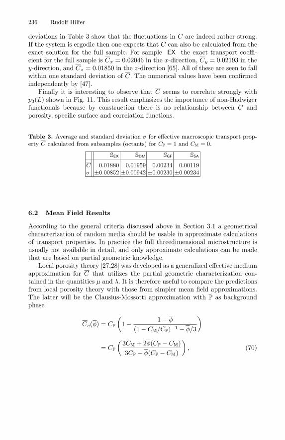
236 Rudolf Hilfer

deviations in Table 3 show that the fluctuations in C are indeed rather strong.If the system is ergodic then one expects that C can also be calculated from theexact solution for the full sample. For sample EX the exact transport coeffi-cient for the full sample is Cx = 0.02046 in the x-direction, Cy = 0.02193 in they-direction, and Cz = 0.01850 in the z-direction [65]. All of these are seen to fallwithin one standard deviation of C. The numerical values have been confirmedindependently by [47].

Finally it is interesting to observe that C seems to correlate strongly withp3(L) shown in Fig. 11. This result emphasizes the importance of non-Hadwigerfunctionals because by construction there is no relationship between C andporosity, specific surface and correlation functions.

Table 3. Average and standard deviation σ for effective macroscopic transport prop-erty C calculated from subsamples (octants) for CP = 1 and CM = 0.

SEX SDM SGF SSA

C 0.01880 0.01959 0.00234 0.00119σ ±0.00852 ±0.00942 ±0.00230 ±0.00234

6.2 Mean Field Results

According to the general criteria discussed above in Section 3.1 a geometricalcharacterization of random media should be usable in approximate calculationsof transport properties. In practice the full threedimensional microstructure isusually not available in detail, and only approximate calculations can be madethat are based on partial geometric knowledge.

Local porosity theory [27,28] was developed as a generalized effective mediumapproximation for C that utilizes the partial geometric characterization con-tained in the quantities µ and λ. It is therefore useful to compare the predictionsfrom local porosity theory with those from simpler mean field approximations.The latter will be the Clausius-Mossotti approximation with P as backgroundphase

Cc(φ) = CP

(1− 1− φ

(1− CM/CP)−1 − φ/3

)

= CP

(3CM + 2φ(CP − CM)3CP − φ(CP − CM)

), (70)


the Clausius-Mossotti approximation with M as background phase

Cb(φ) = CM

(1− φ

(1− CP/CM)−1 − (1− φ)/3

)

= CM

(2CM + CP + 2φ(CP − CM)2CM + CP − φ(CP − CM)

), (71)

and the self-consistent effective medium approximation [35,37]

φCP − CCP + 2C

+ (1− φ) CM − CCM + 2C

= 0 (72)

which leads to a quadratic equation for C. The subscripts b and c in (71) and (70)stand for ”blocking” and ”conducting”. In all of these mean field approximationsthe porosity φ is the only geometric observable representing the influence ofthe microstructure. Thus two microstructures having the same porosity φ arepredicted to have the same transport parameter C. Conversely, measurement ofC combined with the knowledge of CM, CP allows to deduce the porosity fromsuch formulae.

If the microstructure is known to be homogeneous and isotropic with bulkporosity φ, and if CP > CM, then the rigorous bounds [8,24,62]

Cb(φ) ≤ C ≤ Cc(φ) (73)

hold, where the upper and the lower bound are given by the Clausius-Mossottiformulae, eqs. (71) and (70). For CP < CM the bounds are reversed.

The proposed selfconsistent approximations for the effective transport coef-ficient of local porosity theory reads [27]

1∫0

Cc(φ)− CCc(φ) + 2C

λ3(φ,L)µ(φ,L)dφ+

1∫0

Cb(φ)− CCb(φ) + 2C

(1− λ3(φ,L))µ(φ,L)dφ = 0

(74)

where Cb(φ) and Cc(φ) are given in eqs. (71) and (70). Note that (74) is stillpreliminary, and a generalization is in preparation. A final form requires general-ization to tensorial percolation probabilities and transport parameters. Equation(74) is a generalization of the effective medium approximation. In fact, it reducesto eq. (72) in the limit L → 0. In the limit L → ∞ it also reduces to eq. (72)albeit with φ in eq. (72) replaced with λ3(φ). In both limits the basic assump-tions underlying all effective medium approaches become invalid. For small Lthe local geometries become strongly correlated, and this is at variance with thebasic assumption of weak or no correlations. For large L on the other hand theassumption that the local geometry is sufficiently simple becomes invalid [27].Hence one expects that formula (74) will yield good results only for interme-diate L. The question which L to choose has been discussed in the literature

238 Rudolf Hilfer

[3,10,12,33,66]. For the results in Table 4 the so called percolation length Lp hasbeen used which is defined through the condition

d2p3dL2

∣∣∣∣L=Lp

= 0 (75)

assuming that it is unique. The idea behind this definition is that at the inflectionpoint the function p3(L) changes most rapidly from its trivial value p3(0) = φ atsmall L to its equally trivial value p3(∞) = 1 at large L (assuming that the porespace percolates). The length Lp is typically larger than the correlation lengthcalculated from G(r) [10,11].

The results obtained by the various mean field approximations are collectedin Table 4 [65,67]. The exact result is obtained by averaging the three valuesfor the full sample EX given in the previous section. The additional geometricinformation contained in µ and λ seems to give an improved estimate for thetransport coefficient.

Table 4. Effective macroscopic transport property C calculated from Clausius-Mossotti approximations (Cc ,Cb), effective medium theory CEMA and local porositytheory CLPT compared with the exact result Cexact (for CP = 1 and CM = 0).

Cc Cb CEMA CLPT Cexact0.094606 0.0 0.0 0.025115 0.020297

ACKNOWLEDGEMENT: Most results reviewed in this paper were obtainedin cooperation with B. Biswal, C. Manwart, J. Widjajakusuma, P.E. Øren, S.Bakke, and J. Ohser. I am grateful to all of them, and to the Deutsche For-schungsgemeinschaft as well as Statoil A/S Norge for financial support.

References

1. Adler, P. (1992): Porous Media (Butterworth-Heinemann, Boston)2. Adler, P., C. Jacquin, C., J. Quiblier (1990): ‘Flow in simulated porous media’,Int.J.Multiphase Flow 16, p. 691

3. Andraud, C., A. Beghdadi, E. Haslund, R. Hilfer, J. Lafait, B. Virgin (1997): ‘Localentropy characterization of correlated random microstructures’, Physica A 235, p.307

4. Bakke, S., P. Øren (1997): ‘3-d pore-scale modeling of sandstones and flow simula-tions in pore networks’, SPE Journal 2, p. 136

5. Barut, A., R. Raczka (1986): Theory of Group Representations and Applications(World Scientific, Singapore)

6. Bear, J. (1972): Dynamics of Fluids in Porous Media (Elsevier Publ. Co., NewYork)

7. Bear, J., A. Verruijt (1987): Modeling Groundwater Flow and Pollution (KluwerAcademic Publishers, Dordrecht)


8. Bergman, D. (1982): ‘Rigorous bounds for the complex dielectric constant of atwo-component composite’, Ann. Phys. 138, p. 78

9. Biswal, B., R. Hilfer (1999): ‘Microstructure analysis of reconstructed porous me-dia’, Physica A 266, p. 307

10. Biswal, B., C. Manwart, R. Hilfer, R. (1998): ‘Threedimensional local porosityanalysis of porous media’, Physica A 255, p. 221

11. Biswal, B., C. Manwart, R. Hilfer, S. Bakke, P. Øren (1999): ‘Quantitative analysisof experimental and synthetic microstructures for sedimentary rock’, Physica A273, p. 452

12. Boger, F., J. Feder, R. Hilfer, R., T. Jøssang (1992): ‘Microstructural sensitivityof local porosity distributions’, Physica A 187, p. 55

13. Bourbie, T., O. Coussy, B. Zinszner (1987): Acoustics of Porous Media (EditionsTechnip, Paris)

14. Bourbie, T., B. Zinszner (1995): ‘Hydraulic and acoustic properties as a functionof porosity in Fontainebleau snadstone’, J.Geophys.Res. 90, p. 11524

15. Bryant, S., D. Mellor, D., C. Cade (1993): ‘Physically representative network mod-els of transport in porous media’, AIChE Journal 39, p. 387

16. Chatzis, I., F. Dullien (1977): ‘Modelling pore structure by 2-d and 3-d networkswith applications to sandstones’, J. of Canadian Petroleum Technology, p. 97

17. Crivelli-Visconti, I. (ed.) (1998): ECCM-8 European Conference on Composite Ma-terials (Woodhead Publishing Ltd, Cambridge)

18. Delfiner, P. (1972): ‘A generalization of the concept of size’, J. Microscopy 95, p.203

19. Diebels, S., W. Ehlers (1996): ‘On fundamental concepts of multiphase micropolarmaterials’, Technische Mechanik 16, p. 77

20. Dullien, F. (1992): Porous Media - Fluid Transport and Pore Structure (AcademicPress, San Diego)

21. Ehlers, W. (1995): ‘Grundlegende Konzepte in der Theorie poroser Medien’, Tech-nical report, Institut f. Mechanik, Universitat Stuttgart, Germany

22. Fatt, I. (1956): ‘The network model of porous media I. capillary pressure charac-teristics’, AIME Petroleum Transactions 207, p. 144

23. Hadwiger, H. (1955): Altes und Neues uber konvexe Korper (Birkhauser, Basel)24. Hashin, Z., S. Shtrikman (1962): ‘A variational approach to the theory of effective

magnetic permeability of multiphase materials’, J. Appl. Phys. 33, p. 312525. Haslund, E., B. Hansen, R. Hilfer, B. Nøst (1994): ‘Measurement of local porosities

and dielectric dispersion for a water saturated porous medium’, J. Appl. Phys. 76,p. 5473

26. Hearst, J., P. Nelson (1985): Well Logging for Physical Properties (McGraw-Hill,New York)

27. Hilfer, R. (1991): ‘Geometric and dielectric characterization of porous media’, Phys.Rev. B 44, p. 60

28. Hilfer, R. (1992): ‘Local porosity theory for flow in porous media’, Phys. Rev. B45, p. 7115

29. Hilfer, R. (1993): ‘Local porosity theory for electrical and hydrodynamical trans-port through porous media’, Physica A 194, p. 406

30. Hilfer, R. (1996): ‘Transport and relaxation phenomena in porous media’, Advancesin Chemical Physics XCII, p. 299

31. Hilfer, R., B. Nøst, E. Haslund, Th. Kautzsch, B. Virgin, B.D. Hansen (1994):‘Local porosity theory for the frequency dependent dielectric function of porousrocks and polymer blends’, Physica A 207, p. 19

240 Rudolf Hilfer

32. Hilfer, R., T. Rage, B. Virgin (1997): ‘Local percolation probabilities for a naturalsandstone’, Physica A 241, p. 105

33. Hilfer, R., J. Widjajakusuma, B. Biswal (1999): ‘Macroscopic dielectric constantfor microstructures of sedimentary rocks’, Granular Matter, in print

34. Katz, A., A. Thompson (1986): ‘Quantitative prediction of permeability in porousrock’, Phys. Rev. B 34, p. 8179

35. Kirkpatrick, S. (1973): ‘Percolation and conduction’, Rev. Mod. Phys. 45, p. 57436. Lake, L. (1989): Enhanced Oil Recovery (Prentice Hall, Englewood Cliffs)37. Landauer, R. (1978): ‘Electrical conductivity in inhomogeneous media’, in: Electri-

cal Transport and Optical Properties of Inhomogeneous Materials, ed. by J. Garland,D. Tanner (American Institute of Physics, New York), p. 2

38. Levitz, P., D. Tchoubar (1992): ‘Disordered porous solids: From chord distributionsto small angle scatterin’, J. Phys. I France 2, p. 771

39. Louis, A. (1989): Inverse und schlecht gestellte Probleme (Teubner, Stuttgart)40. Manwart, C., R. Hilfer (1999a): to be published41. Manwart, C., R. Hilfer (1999b): ‘Reconstruction of random media using Monte

Carlo methods’, Physical Review E 59, p. 559642. Manwart, C., S. Torquato, R. Hilfer (1999): ‘Stochastic reconstruction of sand-

stones’, preprint43. Marsily, G. (1986): Quantitative Hydrogeology – Groundwater Hydrology for Engi-

neers (Academic Press, San Diego)44. Mecke, K. (1998): ‘Integral geometry and statistical physics’, Int. J. Mod. Phys. B

12, p. 86145. Mecke, K., H. Wagner (1991): ‘Euler characteristic and related measures for ran-

dom geometric sets’, J. Stat. Phys. 64, p. 84346. Muche, L., D. Stoyan (1992): ‘Contact and chord length distributions of the poisson

voronoi tessellation’, Journal of applied probability 29, p. 46747. Øren, P. (1999): private communication48. Øren, P., S. Bakke, O. Arntzen (1998): ‘Extending predictive capabilities to net-

work models’, SPE Journal, p. SPE 3888049. Quiblier, J. (1984): ‘A new three dimensional modeling technique for studying

porous media’, J. Colloid Interface Sci. 98, p. 8450. Roberts, A. (1997): ‘Statistical reconstruction of three-dimensional porous media

from two-dimensional images’, Phys.Rev.E 56, p. 320351. Roberts, J., L. Schwartz (1985): ‘Grain consolidation and electrical conductivity

in porous media’, Phys. Rev. B 31, p. 599052. Roy, D. (1991): Methods of Inverse problems in Physics (CRC Press, Boca Raton)53. Roy, S., S. Tarafdar, S. (1997): ‘Archies’s law from a fractal model for porous rock’,

Phys.Rev.B 55, p. 803854. Sahimi, M. (1993): ‘Flow phenomena in rocks: From continuum models to fractals,

percolation, cellular automata and simulated annealing’, Rev. Mod. Phys. 65, p.1393

55. Sahimi, M. (1995): Flow and Transport in Porous Media and Fractured Rock (VCHVerlagsgesellschaft mbH, Weinheim)

56. Scheidegger, A. (1974): The Physics of Flow Through Porous Media (University ofToronto Press, Toronto)

57. Schneider, R. (1993): Convex Bodies: The Brunn-Minkowski Theory (CambridgeUniversity Press, Cambridge)

58. Schneider, R., W. Weil (1992): Integralgeometrie (Teubner, Stuttgart)59. Schwartz, L., S. Kimminau (1987): ‘Analysis of electrical conduction in the grain

consolidation model’, Geophysics 52, p. 1402


60. Stell, G. (1985) ‘Mayer-Montroll equations (and some variants) through history forfun and profit’, in: The Wonderful World of Stochastics, ed. by M. Shlesinger, G.Weiss (Elsevier, Amsterdam), p. 127

61. Stoyan, D., W. Kendall, J. Mecke (1987): Stochastic Geometry and its Applications(Akademie-Verlag / Wiley, Berlin / Chichester)

62. Torquato, S. (1991): ‘Random heterogeneous media: Microstructure and improvedbounds on effective properties’, Applied mechanics reviews 44, p. 37

63. Torquato, S., G. Stell (1982): ‘Microstructure of Two Phase Random Media I: Then-Point Probability Functions’, J. Chem. Phys. 77, p. 2071

64. Virgin, B., E. Haslund, R. Hilfer (1996): ‘Rescaling relations between two- and threedimensional local porosity distributions for natural and artificial porous media’,Physica A 232, p. 1

65. Widjajakusuma, J., B. Biswal, R. Hilfer (1999a): ‘Predicting transport parametersof heterogeneous media’, preprint

66. Widjajakusuma, J., B. Biswal, R. Hilfer (1999b): ‘Quantitative prediction of effec-tive material properties of heterogeneous media’, Comp. Mat. Sci. 16, p. 70

67. Widjajakusuma, J., R. Hilfer (2000): ‘Local Porosity Theory for Sound Propagationin Porous Media’

68. Widjajakusuma, J., C. Manwart, B. Biswal, R. Hilfer (1999): ‘Exact and approxi-mate calculations for conductivity of sandstones’, Physica A 16, p. 70

69. Yao, J., P. Frykman, F. Kalaydjian, P. Thovert, P. Adler (1993): ‘High-order mo-ments of the phase function for real and reconstructed model porous media: Acomparison’, J. of Colloid and Interface Science 156, p. 478

70. Yeong, C., S. Torquato (1998): ‘Reconstructing random media’, Phys.Rev. E 57,p. 495

71. Ziman, J. (1982): Models of Disorder (Cambridge University Press, Cambridge)

local porosity theory and stochastic reconstruction for...

Documents