local oscillator contribution to …tycho.usno.navy.mil/ptti/2009papers/paper47.pdflocal oscillator...
TRANSCRIPT
41st Annual Precise Time and Time Interval (PTTI) Meeting
537
LOCAL OSCILLATOR CONTRIBUTION
TO CARRIER-PHASE MEASUREMENTS
IN A GNSS RECEIVER
E. Detoma, L. Bonafede, and P. Capetti
SEPA S.p.A.
Via Andrea Pozzo, 8, 10141 Torino, Italy
Abstract
When performing carrier-phase measurements, the measurement noise affecting the
observations reflects two contributions, originating from the thermal noise of the RF signal
received at the antenna and from the stability of the local oscillator over the integration time,
since normally some form of phase-locked loop (PLL) is used for carrier recovery. The order of
the PLL (and the bandwidth) determines the amount of the oscillator contribution to the
measurement noise for a given oscillator frequency stability (or, since the integration time is
generally less or equal to 1 s, to its phase noise). Therefore, it is important to understand the
mechanism by which the local oscillator instability is transferred to the carrier-phase
measurement noise and select a proper oscillator to minimize such a contribution.
In the paper, we will address these issues, providing examples that guide the selection of the
local oscillator. A practical example of implementation will be discussed, where a low-cost,
high-stability OCXO has been disciplined to a Rb frequency standard to provide improved
stability over the integration times of interest in order to minimize the noise for carrier-phase
recovery.
CARRIER-PHASE TRACKING AND LOCAL OSCILLATOR
CONTRIBUTION
In the following, our aim is to define a model, and determine the contributions, for the stochastic errors
affecting the performance of the typical GPS (GNSS) receiver. We will consider errors on pseudorange
and carrier-phase measurements. Under our assumptions, we will consider the receiver as a measurement
instrument, with the target of providing the required measurement (carrier phase or pseudorange) with the
best precision.
Considering pseudorange and carrier-phase measurements, we realize that both are affected by the
received signal-to-noise ratio, by the receiver implementation (and corresponding implementation losses
as respect to theoretical), and by the local oscillator. Let’s start by looking at the received signal-to-noise
ratio.
41st Annual Precise Time and Time Interval (PTTI) Meeting
538
RECEIVED SIGNAL-TO-NOISE RATIO
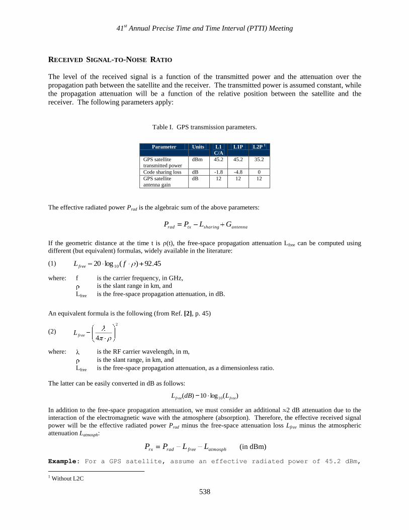
The level of the received signal is a function of the transmitted power and the attenuation over the
propagation path between the satellite and the receiver. The transmitted power is assumed constant, while
the propagation attenuation will be a function of the relative position between the satellite and the
receiver. The following parameters apply:
Table I. GPS transmission parameters.
Parameter Units L1
C/A
L1P L2P 1
GPS satellite transmitted power
dBm 45.2 45.2 35.2
Code sharing loss dB -1.8 -4.8 0
GPS satellite
antenna gain
dB 12 12 12
The effective radiated power Prad is the algebraic sum of the above parameters:
antennasharingtxrad GLPP
If the geometric distance at the time t is (t), the free-space propagation attenuation Lfree can be computed using
different (but equivalent) formulas, widely available in the literature:
(1) 45.92)(log20 10 fL free
where: f is the carrier frequency, in GHz,
is the slant range in km, and
Lfree is the free-space propagation attenuation, in dB.
An equivalent formula is the following (from Ref. [2], p. 45)
(2)
2
4freeL
where: is the RF carrier wavelength, in m,
is the slant range, in km, and
Lfree is the free-space propagation attenuation, as a dimensionless ratio.
The latter can be easily converted in dB as follows:
)(log10)( 10 freefree LdBL
In addition to the free-space propagation attenuation, we must consider an additional 2 dB attenuation due to the
interaction of the electromagnetic wave with the atmosphere (absorption). Therefore, the effective received signal
power will be the effective radiated power Prad minus the free-space attenuation loss Lfree minus the atmospheric
attenuation Latmosph:
atmosphfreeradrx LLPP (in dBm)
Example: For a GPS satellite, assume an effective radiated power of 45.2 dBm,
1 Without L2C
41st Annual Precise Time and Time Interval (PTTI) Meeting
539
a code sharing loss of -1.8 dB, and an antenna gain of 12 dB: the effective
radiated power is 55.4 dBm.
Given a slant range of 25149.567 km, at the L1 frequency (1575 MHz) the
free-space propagation attenuation is -184.406 dB, and the received signal
power level is -129.006 dBm, to be further reduced by -2 dB because of
atmospheric attenuation, so that the effective received signal level at the
receiver antenna will be -131.006 dBm.
The receiving antenna detects the signal with a gain that is a function of the polar radiation diagram of the
antenna itself. If the elevation angle for the satellite is E, the corresponding antenna gain is Gant(E) (we
assume this is a function of E only). Therefore, from geometric considerations based on the relative
position of satellite and receiver, E can be computed and Gant(E) determined.
The input signal power to the receiver Pin at the antenna output2 is again the algebraic sum of the received
signal level Prx in dBm and if the antenna gain, in dB:
)(EGPP antrxin
Example: following the previous example, assuming Prx = -131.006 dBm and an
antenna gain of –3 dB at 5° elevation, the signal power Pin at the output of
the receiving antenna will be Pin = -134.006 dBm.
The noise at the input of the receiver is a complex function of many parameters, including the antenna
noise temperature, the attenuation introduced by the cable connecting the antenna to the receiver, the gain
and noise figure of the low-noise amplifier (LNA) that follows the antenna, and the noise figure of the
receiver itself. To simplify, we can consider a single parameter, generally provided by the manufacturer,
that characterizes the noise performance of the receiver with respect to an ideal receiver.
This parameter is the receiver noise equivalent temperature Tnoise, and we assume3, for instance, that Tnoise
= 238.941 °K. This value is everything we need, assuming that the noise temperature of the antenna, the
noise figure of the LNA, and the length and characteristics (attenuation) of the antenna cable remain
constant.
From the equivalent noise temperature Tnoise, it is straightforward to compute the equivalent noise power
spectral density Pnoise, that can be regarded as the equivalent noise power in a unit bandwidth (1 Hz):
)(log10 10 kTP noisenoise in dBW
30)(log10 10 kTP noisenoise in dBm
where 23103807.1k is the Boltzmann constant. For Tnoise = 238.941 °K, the corresponding noise power
spectral density is -174.816 dBm/Hz.
Now, the ratio C/N0 (in dB/Hz) between the signal (carrier) and the noise will be simply the difference between the
available signal power Pin = -134.006 dBm and the noise power Pnoise = -174.816 dBm/Hz:
2 For the time being, we consider the antenna output as the input of the receiver, assuming that the cable connecting the antenna
to the receiver as an integral part of the receiver itself. The reason will be apparent in the discussion that follows. 3 This is a value measured for a very good geodetic-quality receiver, and applies both to L1 and L2.

41st Annual Precise Time and Time Interval (PTTI) Meeting
540
dB/Hz 40.81816.174006.134
/ 0 noisein PPNC
For an ideal receiver, this value is not degraded by the receiver implementation. In practice, a real receiver
introduces implementation losses with respect to the mechanization of an ideal receiver, a degradation which is due
to losses in the amplification, mixing, and sampling circuits. This additional degradation is known as
implementation loss Limplem and results in a further degradation in the C/N0 ratio. Assume that Limplem = -3 dB. Then
the effective C/N0 ratio will be less than theoretical because of this implementation loss:
dB/Hz .8173
)/( 0 implemnoiseineffective LPPNC
This is the value of C/N0 (in dB/Hz) that we will use in the following. For a given receiver, where the majority of
the above-mentioned parameters can be considered as constant, this value will be a function of the slant range and
elevation angle (for the antenna gain).
ESTIMATION OF THE NOISE AFFECTING THE CARRIER-PHASE MEASUREMENTS
The noise affecting the carrier-phase measurements can be estimated by generalizing the theory of phase-locked
loops (PLLs), since we can consider the receiver as using some form of a Costas loop to reconstruct the suppressed
carrier. It can be shown that other methods (based, for instance, on the squaring of the signal to recover the
suppressed carrier) produce theoretically equivalent results, and therefore the results that are presented in the
following are implementation-independent (except for the implementation losses introduced by the practical
implementation, obviously).
The noise affecting the phase measurements on the recovered carrier consists in the sum of two contributions, the
thermal noise affecting the RF input signal and the stability of the local oscillator (since any phase measurement is
always relative):
22
LOthermalphase
The two contributions will be separately analyzed.
CONTRIBUTION DUE TO THE STABILITY OF THE LOCAL OSCILLATOR The time error (jitter) t produced over an interval because of the instability of the local oscillator is:
)()( yt (in seconds)
where )(y is a measure of the frequency instability of the oscillator expressed as the Allan variance of the
fractional frequency fluctuations4. For a phase-locked loop, the characteristic time interval can be considered as
the inverse of the loop bandwidth BL:
LB
1
where we are, for the time being, neglecting the loop filter actual transfer function and considering an ideal
response:
4 I.e.: f/f.
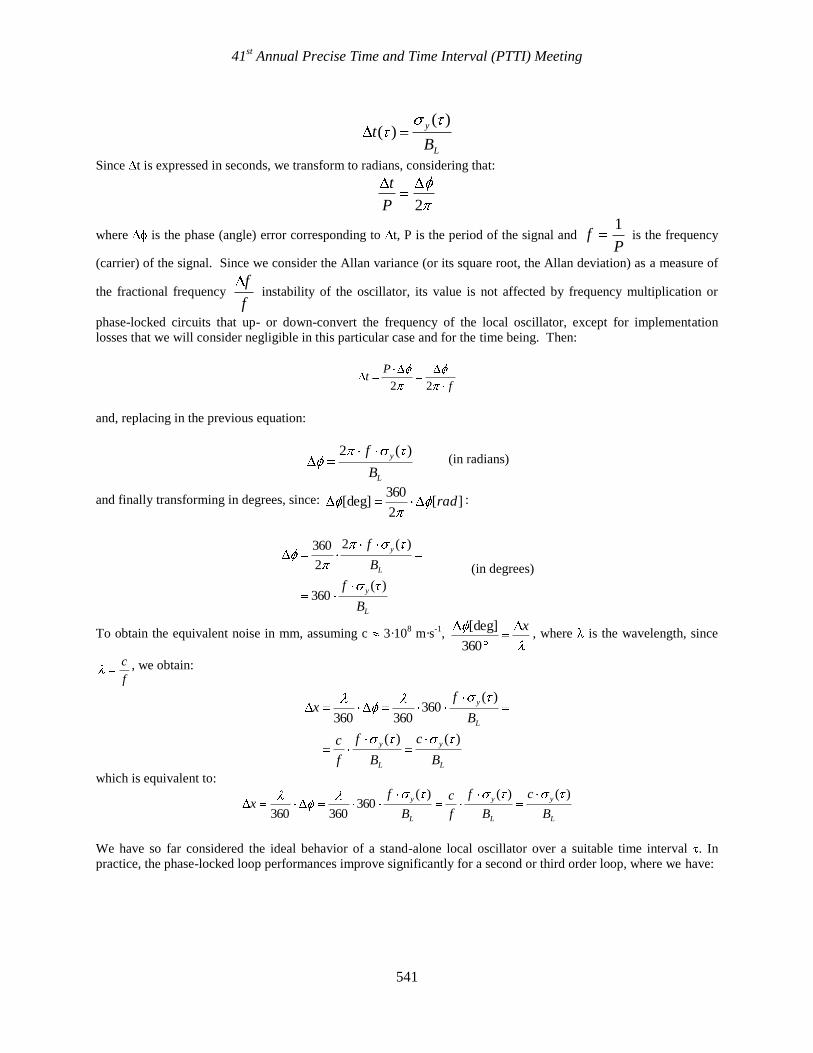
41st Annual Precise Time and Time Interval (PTTI) Meeting
541
L
y
Bt
)()(
Since t is expressed in seconds, we transform to radians, considering that:
2P
t
where is the phase (angle) error corresponding to t, P is the period of the signal and P
f1
is the frequency
(carrier) of the signal. Since we consider the Allan variance (or its square root, the Allan deviation) as a measure of
the fractional frequency f
f instability of the oscillator, its value is not affected by frequency multiplication or
phase-locked circuits that up- or down-convert the frequency of the local oscillator, except for implementation
losses that we will consider negligible in this particular case and for the time being. Then:
f
Pt
22
and, replacing in the previous equation:
L
y
B
f )(2 (in radians)
and finally transforming in degrees, since: ][2
360[deg] rad :
L
y
L
y
B
f
B
f
)(360
)(2
2
360
(in degrees)
To obtain the equivalent noise in mm, assuming c 3·108 m·s
-1,
x
360
[deg], where is the wavelength, since
f
c , we obtain:
L
y
L
y
L
y
B
c
B
f
f
c
B
fx
)()(
)(360
360360
which is equivalent to:
L
y
L
y
L
y
B
c
B
f
f
c
B
fx
)()()(360
360360
We have so far considered the ideal behavior of a stand-alone local oscillator over a suitable time interval . In
practice, the phase-locked loop performances improve significantly for a second or third order loop, where we have:
41st Annual Precise Time and Time Interval (PTTI) Meeting
542
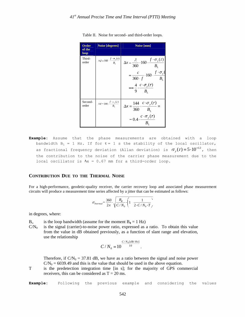
Table II. Noise for second- and third-order loops.
Order
of the
loop
Noise [degrees] Noise [mm]
Third-
order L
y
B
f )(160
L
y
L
y
L
y
B
c
B
f
f
c
B
fx
)(
9
4
)(160
360
)(160
360
Second-
order L
y
B
f )(144
L
y
L
y
B
c
B
cx
)(4.0
)(
360
144
Example: Assume that the phase measurements are obtained with a loop
bandwidth BL = 1 Hz. If for = 1 s the stability of the local oscillator,
as fractional frequency deviation (Allan deviation) is 12105)(y , then
the contribution to the noise of the carrier phase measurement due to the
local oscillator is x = 0.67 mm for a third-order loop.
CONTRIBUTION DUE TO THE THERMAL NOISE
For a high-performance, geodetic-quality receiver, the carrier recovery loop and associated phase measurement
circuits will produce a measurement time series affected by a jitter that can be estimated as follows:
TNCNC
Bthermal
00 /2
11
/2
360
in degrees, where:
B is the loop bandwidth (assume for the moment B = 1 Hz)
C/N0 is the signal (carrier)-to-noise power ratio, expressed as a ratio. To obtain this value
from the value in dB obtained previously, as a function of slant range and elevation,
use the relationship
10
]/[/
0
0
10/
HzdBNC
NC .
Therefore, if C/N0 = 37.81 dB, we have as a ratio between the signal and noise power
C/N0 = 6039.49 and this is the value that should be used in the above equation.
T is the predetection integration time [in s]; for the majority of GPS commercial
receivers, this can be considered as T = 20 ms.
Example: Following the previous example and considering the values
41st Annual Precise Time and Time Interval (PTTI) Meeting
543
obtained so far, we have: C/N0 = 37.81 dB/Hz, T = 20 ms, and B = 1 Hz. Under
these assumptions, the thermal noise contribution to the jitter affecting
the carrier-phase measurements is x = 0.39 mm. Notice how this value is
significantly less to the contribution due to the local oscillator with a
frequency stability of 12105)(yat 1 s, that is already a very good
frequency stability. Adding the two contributions, respectively, due to the
local oscillator instability and to the thermal noise, the resulting jitter
affecting the carrier-phase measurements results in 0.773 mm, where the
dominant term is due to the local oscillator.
PSEUDORANGE MEASUREMENTS NOISE (CODE, SS-PRN) Two models will be considered: the first to estimate the theoretical performance that can be obtained from the GPS
code measurements using a Minimum Value Unbiased Estimator (MVUE) and the second to estimate the
performance that can be obtained by a digital non-coherent Early-minus-Late phase-locked loop.
MINIMUM VALUE UNBIASED ESTIMATOR [MVUE]
Make use of the following relationship (cf. Ref. [6], Eq. 2-21, p. 137):
c
WN
Ck
Tm
C
MVUEcode
0
,
2
4
1][
where:
Wc is the signal (code) bandwidth (Wc = 1.024 MHz for a typical receiver)
C/N0 is the signal (carrier)-to-noise power ratio, expressed as a ratio. To obtain this value from the value
in dB obtained previously, as a function of slant range and elevation, use the relationship
10
]/[/
0
0
10/
HzdBNC
NC
Therefore, if C/N0 = 37.81 dB we have as a ratio between the signal and noise power C/N0 =
6039.49 and this is the value that should be used in the above equation.
T is the integration (observation) time for the signal [in s]; let T = 0.02 s
k is a constant:
k = 512·103 for the GPS C/A code
k = 512·104 for the GPS P code
c is the speed of propagation of the light “in vacuum.”
Wc, k and T can be considered constant parameters, while C/N0 should be computed from the slant range and the
elevation, the latter to keep into account the antenna gain.
Example: Following the previous example, let C/N0 = 37.81 dB/Hz, Wc = 1.024
MHz, T = 0.02 s, and k = 512·103 (C/A code); the jitter affecting the
pseudorange measurements is 0.27 m.
DIGITAL NON-COHERENT “EARLY-MINUS-LATE” PHASE-LOCKED LOOP
The equation (cf. Ref. [1], p. 14) models the jitter standard deviation for a digital non-coherent “Early-
minus-Late” phase-locked loop:

41st Annual Precise Time and Time Interval (PTTI) Meeting
544
TN
Sd
N
S
dBLDLL
00
)2(
21
2
where:
BL is the loop bandwidth (let BL = 10 Hz)
S/N0 is the signal (carrier)-to-noise power ratio, expressed as a ratio. To obtain this value from the value
in dB obtained previously, as a function of slant range and elevation, use the relationship
10
]/[/
0
0
10/
HzdBNC
NC .
Therefore, if C/N0 = 37.81 dB, we have as a ratio between the signal and noise power C/N0 =
6039.49 and this is the value that should be used in the above equation.
T is the predetection filter integration time [in s]; let T = 20 ms unless otherwise specified
d is the correlator resolution, expressed in chips of the PRN code.
Multiplying the above result for the chip period and for the value of the speed of light in free-space we obtain the
standard deviation on the pseudorange measurement5:
TN
Sd
N
S
dBcTcTm L
ccDLLP
00
)2(
21
2
][
where: Tc is the chip period (Tc = 1/1.024 MHz for the C/A code)
c is the speed of light in free space.
Example: Following the previous example and using the same parameters, C/N0 =
37.81 dB/Hz, Tc = 1/1.024 MHz, let BL = 10 Hz and d = 0.14 (C/A code); then
the jitter affecting the C/A code pseudorange measurements is 3.18 m.
The above equation should not be used for P-code measurements on commercial geodetic receivers, since it will
certainly provide optimistic results. The decrease in the chip period (Tc = 1/10.24 MHz for the P code) is only
partially compensated by the change in S/N0 ratio, generally around–3 dB at low elevations, while the equation does
not account6 for the implementation losses due to “code-less” correlation techniques used for P1. For P2 there is a
significative increase in the implementation losses, as will be shown in the next section.
IMPLEMENTATION LOSSES FOR CODELESS P2 TRACKING
A description of the existing techniques is given in the excellent paper by K. T. Woo [5]. The implementation loss
for the most commonly used techniques is given in (Figure 1). The “Z-tracking” appears to be the most efficient
technique among those considered.
5 Cf. also Ref. [0], p. 169. 6 Consider that, for P1, the carrier can be recovered from the C/A code recovery loop; this is not possible for P2 on L2 without
L2C.

41st Annual Precise Time and Time Interval (PTTI) Meeting
545
Figure 1. Implementation loss in P2 codeless recovery (from Ref. [5]).
For the “Z-tracking” technique, between 25 and 50 dB-Hz the loss appears sufficiently linear to justify a
linear approximation to model it:
02 /53 NCLossL [in dB]
where both LossL2 and C/N0 are expressed in dB. The jitter affecting the carrier-phase and the code
measurements can be estimated using the previous equations by further degrading the implementation
loss of the receiver by the contribution due to LossL2.
GALILEO CODE TRACKING
L1 BOC(1,1) CODE ANALYSIS Galileo performances are expected to be markedly improved at L1 by the use of the BOC (1,1)
7 versus the BPSK
modulation used by the GPS C/A code at L1. The advantage is in that, while the useful bandwidth is the same, the
BPSK spectrum is centered around the carrier, while the BOC spectrum is split apart from the suppressed carrier,
effectively occupying a bandwidth extending from 1 to 2 MHz from the carrier.
The approximate expression for the expected noise at L1 for Galileo BOC (1,1) signal as given in Refs. [7] and [8]
as:
(3)
TN
Cd
N
C
dBT L
cC
00
)2(
21
23
1
A close inspection of Eq. (3) shows that the equation is identical to the GPS BPSK performance (except for the term
c, which simply translates the timing uncertainty into ranging uncertainty) and the factor 3
1 , which represents the
7 Now is MBOC.
41st Annual Precise Time and Time Interval (PTTI) Meeting
546
expected improvement of the BOC Galileo modulation over the BPSK GPS modulation. In practice, we expect an
even greater improvement because of the added transmitted RF power from the Galileo satellites, which contributed
to an improved C/N0 ratio. But, as a minimum, we can safely assume just an improvement in performances of a
factor 3
1 = 1.7.
E5A SIGNAL ANALYSIS The expression for the pseudo-range code noise on E5a is slightly more complex than for the BOC(1,1) at L1.
Again, from Refs. [7] and [9], the precision of the measurements is given as:
(4)
TN
Cd
bd
b
b
N
C
BT L
cC
0
2
0
)2(
21
1
1
1
2
.
As you can notice from a close inspection of Eqs. (3) and (4), the term d at the numerator of the first term under
square root has been replaced by the following term:
2
1
1
1
bd
b
b
where b is the normalized front-end bandwidth and we assume as usual that BL·T << 1.
The conclusions of the previous analysis are summarized in Table III. The values reported are those computed in
the numerical example used in the previous sections, corresponding to a worst-case example (low elevation).
It is clear that the selection of the local oscillator is critical to the precision in the carrier-phase measurements; notice
that, even with a stability of 5·10-12
, the dominant contribution to the carrier-phase measurement noise remains the
local oscillator. The contributions (local oscillator and thermal noise) become equivalent only for a stability close to
1·10-12
, where both are in the order of 0.4 mm. Therefore, it is very important to ensure the stability of the local
oscillator under these circumstances not to degrade, as far as possible, the precision of the measurements.
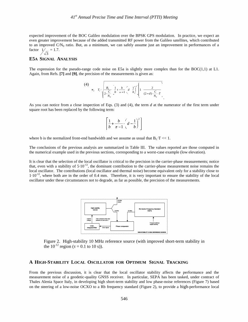
High-stability
OCXORb Atomic Frequency Standard
RAFS
Phase comparatorLoop
integrator/filter
10 MHz 10 MHz
10 MHz
output
Error signal
Control
voltage
HIGH-STABILITY 10 MHz REFERENCE SOURCE
Time constant of the loop
between 10 and 100 s
Frequency/phase
digital steering
High-stability
OCXORb Atomic Frequency Standard
RAFS
Phase comparatorLoop
integrator/filter
10 MHz 10 MHz
10 MHz
output
Error signal
Control
voltage
HIGH-STABILITY 10 MHz REFERENCE SOURCE
Time constant of the loop
between 10 and 100 s
Frequency/phase
digital steering
Figure 2. High-stability 10 MHz reference source (with improved short-term stability in
the 10-12
region (τ = 0.1 to 10 s)).
A HIGH-STABILITY LOCAL OSCILLATOR FOR OPTIMUM SIGNAL TRACKING From the previous discussion, it is clear that the local oscillator stability affects the performance and the
measurement noise of a geodetic-quality GNSS receiver. In particular, SEPA has been tasked, under contract of
Thales Alenia Space Italy, in developing high short-term stability and low phase-noise references (Figure 7) based
on the steering of a low-noise OCXO to a Rb frequency standard (Figure 2), to provide a high-performance local

41st Annual Precise Time and Time Interval (PTTI) Meeting
547
oscillator for GNSS receivers applications within the Galileo Test Range (GTR) in Rome.
The phase-locked loop is used to combine the medium-term stability of the Rb oscillator (this is a high-performance
SpectraTime LPFRS-01 Rb oscillator; see Figure 3) with the excellent short-term stability of a Morion MV89
double-oven OCXO (Figure 4).
Figure 3. Rb oscillator, 10 MHz output, stand-alone.
Figure 4. MV89 OCXO, 10 MHz output stability, stand-alone.
The optimum locking point, designed by an appropriate choice of the loop bandwidth, is at the point in
which the stability of the RB oscillator alone intersects the stability of the OCXO oscillator alone (Figure
5).
In practice, the point must be selected by assuming also the degradation in stability of the two oscillators
due to the environmental conditions, and will be generally for a shorter time constant than the one
dictated by stability in optimum conditions alone. This is to account for the inevitable degradation in
frequency stability when the oscillators operate in real-world conditions.

41st Annual Precise Time and Time Interval (PTTI) Meeting
548
Frequency stability (Rb oscillator and OCXO)
1.00E-13
1.00E-12
1.00E-11
1.00E-10
0.1 1 10 100 1000 10000
Sampling time (s)F
req
uen
cy s
tab
ilit
y
Rb oscillator stability
OCXO stability
Optimum time constant
for the PLL loop
Figure 5. Frequency stability for a Rb oscillator and a high-stability OCXO.
The result is the stability performance for the combined oscillator shown in Figure 6. The frequency stability
improvement is dramatic with respect to the Rb alone in the region for t < 1 s. From 100 ms to 1 s, the stability of
the 10 MHz output of the combined oscillator is below 4·10-12
. The data were taken at INRiM in Torino against an
H-maser, so the contribution of the local reference is negligible and the plot shows the actual stability of the
combined OCXO+Rb oscillator only.
Figure 6. OCXO locked to Rb.
CONCLUSIONS The optimum selection of the local oscillator for a high-quality GNSS receiver is very important and extremely
critical to reduce the noise and improve the precision of carrier-phase measurements. When a single oscillator does
not provide all the required characteristics, the solution can still be found by combining more than one oscillator to
achieve the desired results.
The original equipment has been developed with analog circuitry because of an extremely stringent deadline in the
procurement. Work is continuing to develop an advanced, redundant version with digital control and more features.
ACKNOWLEDGMENTS The author is grateful to Thales Alenia Space Italy for the initial stimulus to investigate the properties of the local
41st Annual Precise Time and Time Interval (PTTI) Meeting
549
oscillator for high-quality geodetic receivers (Thales Alenia Space Italy, Milan and Turin plants, in support to the
ESA GOCE satellite mission) and for the support provided (Thales Alenia Space, Rome) by funding this
development in the framework of the GTR activities, to the colleagues of INRiM for the help in testing the
equipment and to the colleagues in SEPA for the help provided in assembling the instruments.
E. Detoma wishes to dedicate this work to the memory of his mother Anna, who passed away while he was writing
it.
REFERENCES [1] L. Marradi, “LAGRANGE receiver: Raw Measurements and Navigation Data Processing Analysis Summary,”
LABEN Technical Note TL17856.
[2] M. S. Grewal, L. R. Weill, and A. P. Andrews, 2001, Global Positioning Systems, Inertial Navigation and
Integration (Wiley Interscience, New York).
[3] “Invitation to tender for SSTI for GOCE Satellite: answers to request for clarification (2),” LABEN fax no. LA-
OF-MK-TF-0878-01 (5 October 2001).
[4] E. D. Kaplan, ed., 1996, Understanding GPS: Principles and Applications (Artech House Tele-
communications Library).
[5] K. T. Woo, 1999, “Optimum Semi-Codeless Carrier Phase Tracking of L2,” in Proceedings of the ION GPS
Meeting, 14-17 September 1999, Nashville, Tennessee, USA (Institute of Navigation, Alexandria, Va.), pp.
289-305.
[6] D. Weill, 1994, “C/A Code Pseudo-ranging Accuracy – How Good Can It Get?” in Proceedings of ION GPS,
20-23 September 1994, Salt Lake City, Utah, USA (Institute of Navigation, Alexandria, Va.), pp. 133-141.
[7] N. Gerein, M. Olynik, M. Clayton, J. Auld, and T. Murfin, 2005, “A dual frequency L1/E5a Galileo Test
receiver,” in Proceedings of the European Navigation Conference GNSS 2005, 19-22 July 2005, Munich,
Germany.
[8] N. Gerein, M. Olynik, and M. Clayton, 2004, “Galileo BOC(1,1) prototype receiver development,” in
Proceedings of ION GNSS Meeting, 21-24 September 2004, Long Beach, California, USA (Institute of
Navigation, Alexandria, Virginia), pp. 2604-2610.
[9] J. W. Betz, 2000, “Design and performance of code tracking for the GPS M-code signal,” in Proceedings of
ION GPS, 19-22 September 2000, Salt Lake City, Utah, USA (Institute of Navigation, Alexandria, Virginia).

41st Annual Precise Time and Time Interval (PTTI) Meeting
550
Table III. Summary of contributions to the noise affecting the carrier-phase and code
measurements (GPS receiver).
Measurement
Contributions Measurement
precision (jitter)
Dominant contribution
Carrier phase Local oscillator
stability 12105)(y
0.7 mm Stability of the local
oscillator
Signal thermal noise - C/N0 =
37.810 dBm/Hz
0.39 mm
Pseudorange
(C/A code)
Local oscillator stability 12105)(y
Negligible Thermal noise
Signal thermal noise - C/N0 =
37.810 dBm/Hz 3 4 m for “Early-
minus-Late” correlator
Figure 7. High-stability frequency reference, inner view showing Rb and OCXO.