Local Feature Detectorsand

Descriptors

CS 6350 – COMPUTER VISION

Overview

• Local invariant features• Keypoint localization

- Hessian detector- Harris corner detector

• Scale Invariant region detection- Laplacian of Gaussian (LOG) detector- Difference of Gaussian (DOG) detector

• Local feature descriptor- Scale Invariant Feature Transform (SIFT)- Gradient Localization Oriented Histogram (GLOH)

• Examples of other local feature descriptors

Motivation• Global feature from the whole image is often not desirable

• Instead match local regions which are prominent to the object or scene in the image.• Application Area

- Object detection- Image matching- Image stitching

Requirements of a local feature

• Repetitive : Detect the same points independently in each image.

• Invariant to translation, rotation, scale.

• Invariant to affine transformation.

• Invariant to presence of noise, blur etc.

• Locality :Robust to occlusion, clutter and illumination change.

• Distinctiveness : The region should contain “interesting” structure.

• Quantity : There should be enough points to represent the image.

• Time efficient.

Others preferable (but not a must):

o Disturbances, attacks,

o Noise

o Image blur

o Discretization errors

o Compression artifacts

o Deviations from the mathematical model(non-linearities, non-planarities, etc.)

o Intra-class variations

General approach

1. Find the interest points.2. Consider the region

around each keypoint.3. Compute a local

descriptor from the region and normalize the feature.

4. Match local descriptors

+

++

+++ ( )

local descriptor

Slide credit: Bastian Leibe

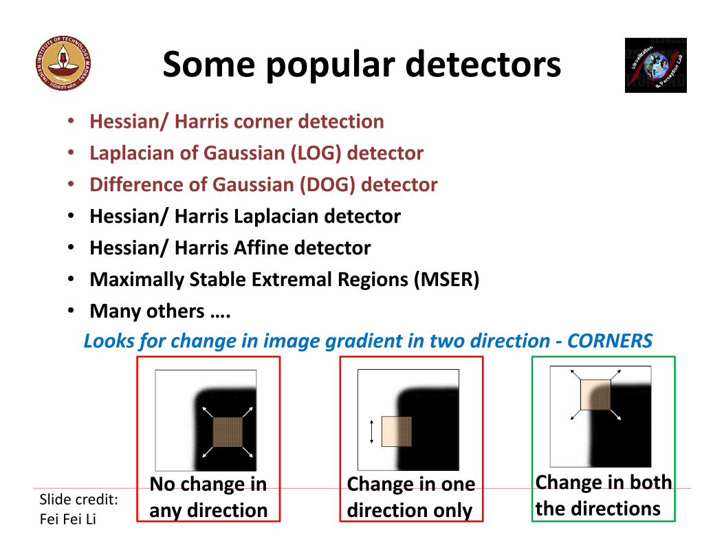
Some popular detectors• Hessian/ Harris corner detection• Laplacian of Gaussian (LOG) detector • Difference of Gaussian (DOG) detector• Hessian/ Harris Laplacian detector• Hessian/ Harris Affine detector• Maximally Stable Extremal Regions (MSER)• Many others ….

Looks for change in image gradient in two direction - CORNERS

Change in both the directions

Change in one direction only

No change in any directionSlide credit:

Fei Fei Li

Hessian Corner Detector[Beaudet, 1978]

Searches for image locations which have strong change in gradient along both the orthogonal direction.

= ),x(I),x(I

),x(I),x(I),x(H

yyxy

xyxx

σσσσ

σ

2xyyyxx III)Hdet( −=

• Perform a non-maximum suppression using a 3*3 window.• Consider points having higher value than its 8 neighbors.

θ>)Hdet( where pointsSelect

Hessian Detector – Result

Effect: Responses mainly on corners and strongly textured areas.

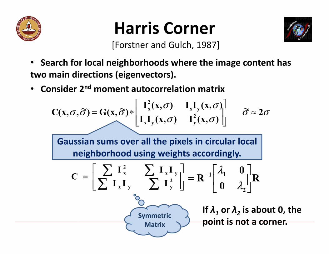
Harris Corner[Forstner and Gulch, 1987]

• Search for local neighborhoods where the image content has two main directions (eigenvectors).• Consider 2nd moment autocorrelation matrix

σσσσσσ

σσσ 2~ ),x(I),x(II),x(II),x(I

)~,x(G)~,,x(C 2yyx

yx2x ≈

∗=

=

2yyx

yx2x

IIIIII

C

Symmetric Matrix

If λ1 or λ2 is about 0, the point is not a corner.

Gaussian sums over all the pixels in circular local neighborhood using weights accordingly.

R0

0R

2

11

= −

λλ

Harris cornerEigen decomposition: visualization

Slide credit: K. Grauman, B. Leibe

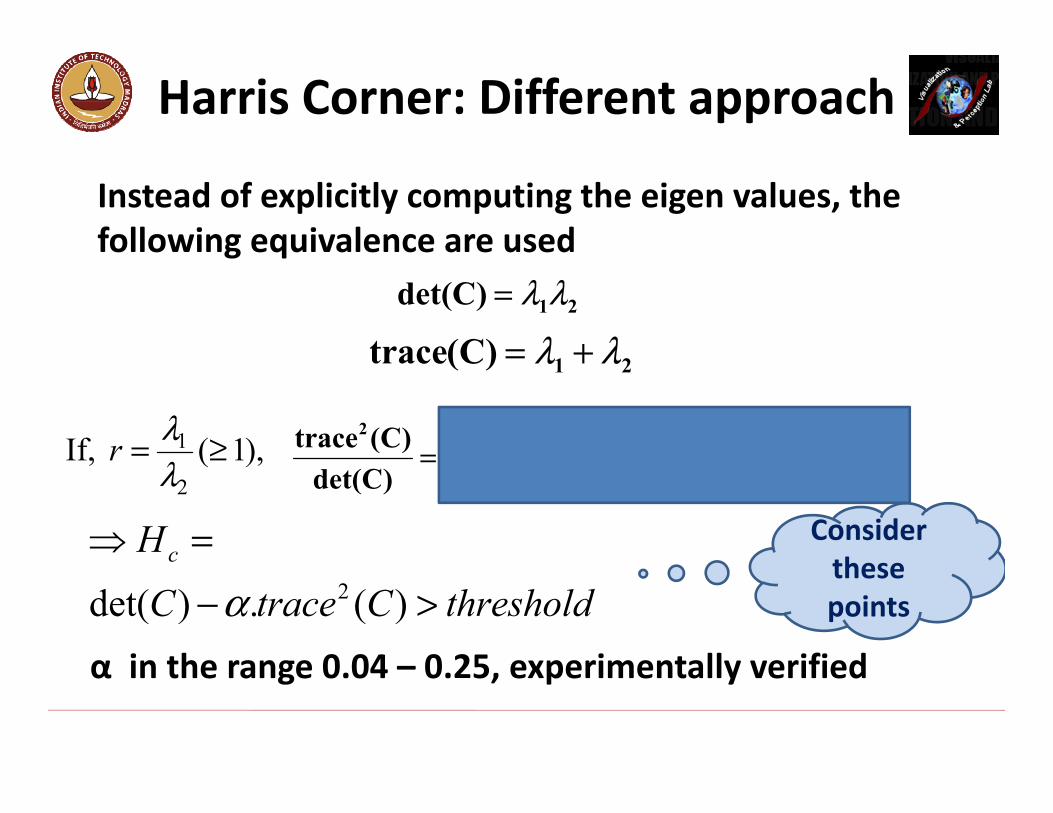
Harris Corner: Different approach

Instead of explicitly computing the eigen values, the following equivalence are used

21)Cdet( λλ=

21)C(trace λλ +=

r)1r(

r)r()(

)Cdet()C(trace 2

22

222

21

221

2 +=+=+=λ

λλλλλλ),1( If,

2

1 ≥=λλr

thresholdCtraceCHc

>−

=

)(.)det( 2α

Consider these points

α in the range 0.04 – 0.25, experimentally verified

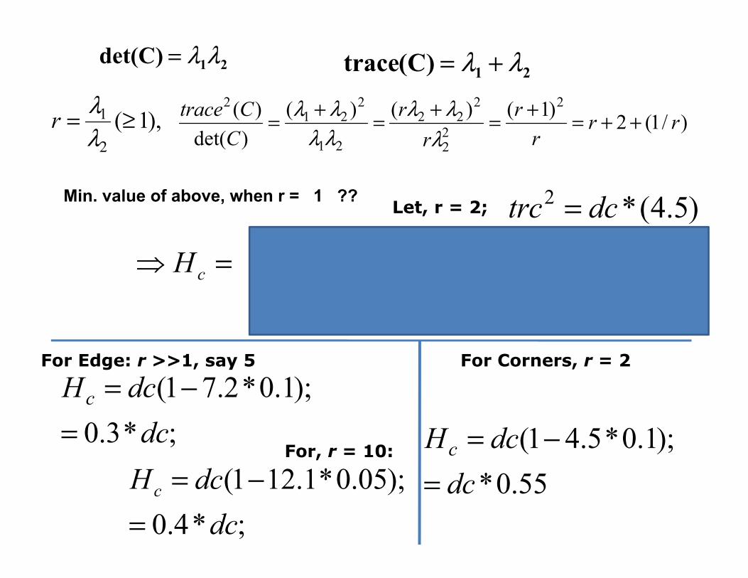
21)Cdet( λλ=21)C(trace λλ +=

)/1(2)1()()()det(

)( 2

22

222

21

221

2rr

rr

rr

CCtrace ++=+=+=+=

λλλ

λλλλ),1(

2

1 ≥=λλr

Let, r = 2; )5.4(*2 dctrc =

);222.0(5.4/1;0);*5.41()(.)det( 2

=<>−=−=

ααα

c

c

HFordcCtraceCH

For Edge: r >>1, say 5 For Corners, r = 2

;*3.0);1.0*2.71(

dcdcHc

=−=

55.0*);1.0*5.41(

dcdcHc

=−=

Min. value of above, when r = 1 ??

For, r = 10:

;*4.0);05.0*1.121(

dcdcHc

=−=

Harris Corner : Example

1. Image derivatives

2. Square of derivatives

3. Gaussian filter G(σI)

Ix Iy

Ix2 Iy

2 IxIy

g(Ix2) g(Iy

2)g(IxIy)

4. Cornerness function – both eigenvalues are strong

Slide credit: K. Grauman, B. Leibe

α = .04 α = .08 α = .1

α = .17 α = .2 α = .25α = .14

CORNERNESS – HARRIS CORNER

Harris Corner : Result

Effect: A very precise corner detector.

Harris Corner

Hessian Detector

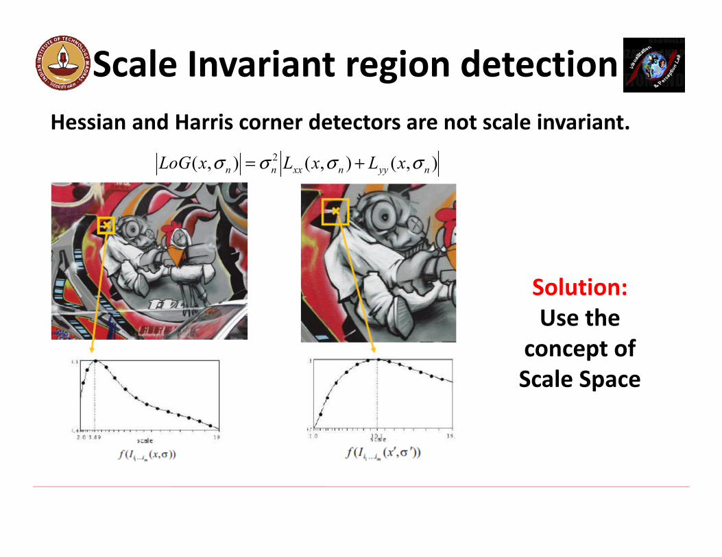
Scale Invariant region detectionHessian and Harris corner detectors are not scale invariant.

Solution:Use the

concept of Scale Space

),(),(),( 2nyynxxnn xLxLxLoG σσσσ +=

Laplacian of Gaussian (LOG) detector [Lindeberg, 1998]

• Using the concept of Scale Space.• Instead of taking zero crossing (for edge detection), consider the point which is maximum among its 26 neighbors (9+9+8).

)),(),((),( 2 σσσσ xIxIxL yyxx +=

• LOG can be used for finding the characteristic scale for a given image location.• LOG can be used for finding scale invariant regions by searching 3D (location + scale) extremaof the LOG.• LOG is also used for edge detection.

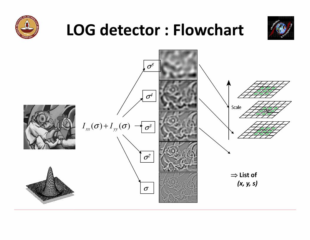
)()( σσ yyxx II +

σ

σ2

σ3

σ4

σ5

List of(x, y, s)

LOG detector : Flowchart

LOG detector : Result

Difference of Gaussian (DOG) Detector [Lowe, 2004]

Approximate LOG using DOG for computational efficiency

)x(I*)),x(G)k,x(G(),x(D

σσσ

−=

k = 21/K

K = 0, 1, 2, … , constant

Consider the region where the DOG response is greater than a threshold and the scale lies in a predefined range [ ]maxmin s,s

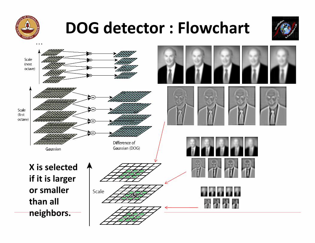
X is selected if it is larger or smaller than all neighbors.

DOG detector : Flowchart

DOG detector : Result

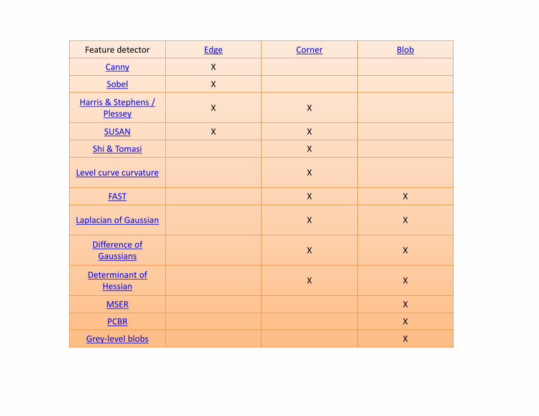
Feature detector Edge Corner Blob

Canny X

Sobel X

Harris & Stephens / Plessey X X

SUSAN X X

Shi & Tomasi X

Level curve curvature X

FAST X X

Laplacian of Gaussian X X

Difference of Gaussians X X

Determinant of Hessian X X

MSER X

PCBR X

Grey-level blobs X

Local Descriptors• We have detected the interest points in an image.• How to match the points across different images of the same object?

Use Local DescriptorsSlide credit: Fei Fei Li

List of local feature descriptors

• Scale Invariant Feature Transform (SIFT)• Speed-Up Robust Feature (SURF)• Histogram of Oriented Gradient (HOG)• Gradient Location Orientation Histogram (GLOH)• PCA-SIFT• Pyramidal HOG (PHOG)• Pyramidal Histogram Of visual Words (PHOW)• Others….(shape Context, Steerable filters, Spin images).

Should be robust to viewpoint change or illumination change

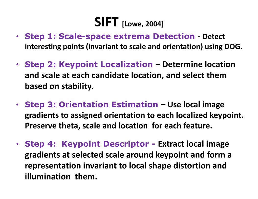
SIFT [Lowe, 2004]• Step 1: Scale-space extrema Detection - Detect

interesting points (invariant to scale and orientation) using DOG.

• Step 2: Keypoint Localization – Determine location and scale at each candidate location, and select them based on stability.

• Step 3: Orientation Estimation – Use local image gradients to assigned orientation to each localized keypoint. Preserve theta, scale and location for each feature.

• Step 4: Keypoint Descriptor - Extract local image gradients at selected scale around keypoint and form a representation invariant to local shape distortion and illumination them.

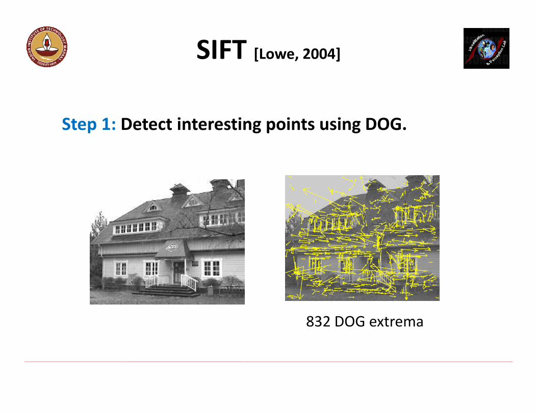
SIFT [Lowe, 2004]

Step 1: Detect interesting points using DOG.

832 DOG extrema

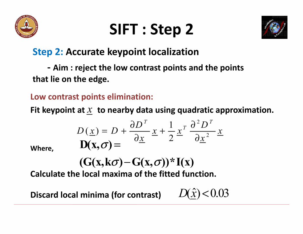
SIFT : Step 2Step 2: Accurate keypoint localization

- Aim : reject the low contrast points and the points that lie on the edge.

Low contrast points elimination:Fit keypoint at to nearby data using quadratic approximation.

Where,

Calculate the local maxima of the fitted function.

Discard local minima (for contrast)

2

21( )2

T TTD DD x D x x x

x x∂ ∂= + +∂ ∂

ˆ( ) 0.03D x <

x

)x(I*)),x(G)k,x(G(),x(D

σσσ

−=

Low contrast points elimination:Fit keypoint at to nearby data using quadratic approximation.

Calculate the local maxima of the fitted function { X = (x, y, σ)}.

2

21( )2

T TTD DD x D x x x

x x∂ ∂= + +∂ ∂

12

2ˆ D Dxx x

−∂ ∂= −∂ ∂

x

=

∂∂+

∂∂=

∂

∂∂+

∂∂+∂

=∂∂ 0

21

2

22

2

xxD

xD

x

xxDxx

xDD

xD

TT

T

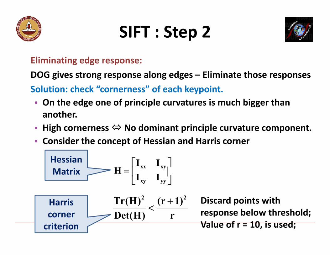
Eliminating edge response:DOG gives strong response along edges – Eliminate those responsesSolution: check “cornerness” of each keypoint.• On the edge one of principle curvatures is much bigger than

another.• High cornerness No dominant principle curvature component.• Consider the concept of Hessian and Harris corner

SIFT : Step 2

=

yyxy

xyxx

IIII

H

r)1r(

)H(Det)H(Tr 22 +<

Hessian Matrix

Harris corner

criterion

Discard points with response below threshold;Value of r = 10, is used;

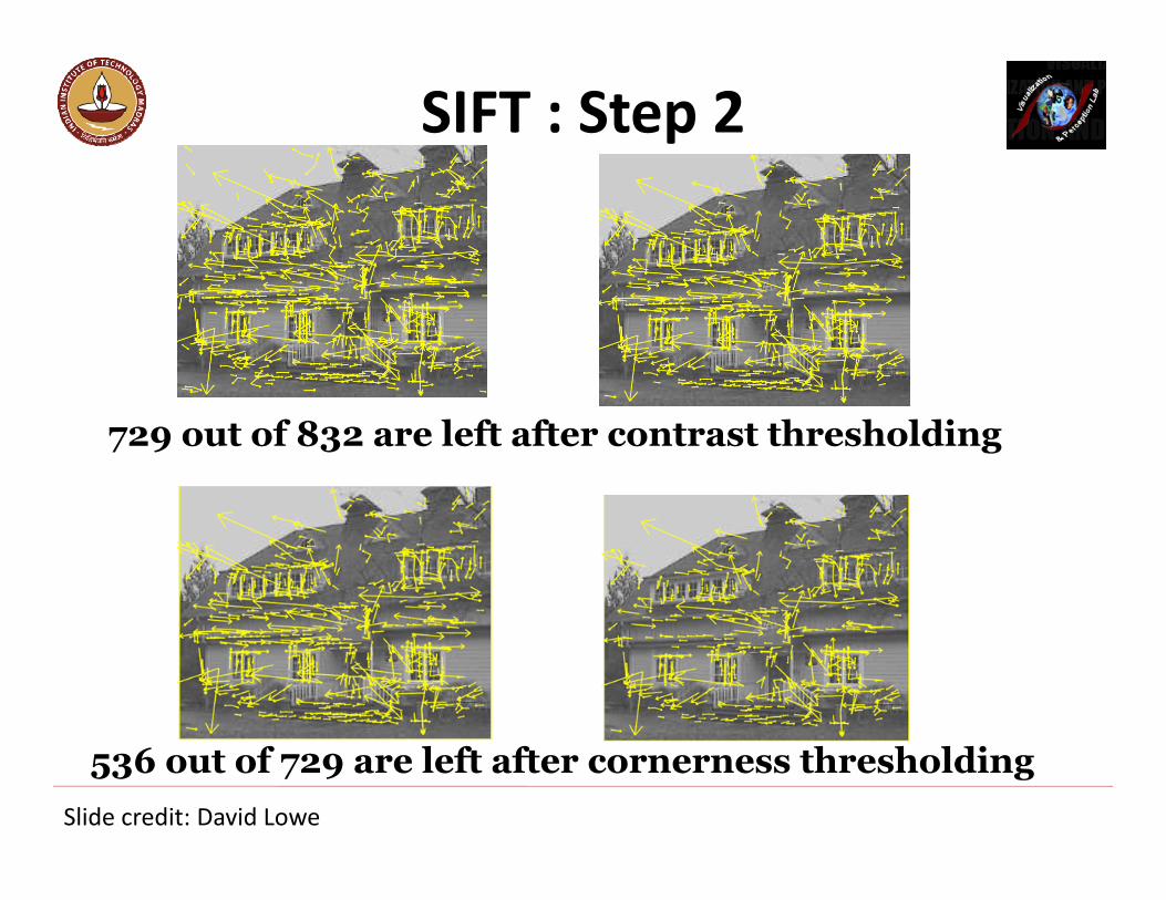
SIFT : Step 2

536 out of 729 are left after cornerness thresholdingSlide credit: David Lowe

729 out of 832 are left after contrast thresholding

SIFT : Step 3Step 3: Orientation Assignment

- Aim : Assign constant orientation to each keypoint based on local image property to obtain rotational invariance.

The magnitude and orientation of gradient of an image patch I(x,y) at a particular scale is:

22 ))1y,x(I)1y,x(I())y,1x(I)y,1x(I()y,x(m −−++−−+=

)y,1x(I)y,1x(I)1y,x(I)1y,x(Itan)y,x( 1

−−+−−+= −θ

To transform relative data accordingly

SIFT : Step 3Step 3: Orientation Assignment

• Create weighted (magnitude + Gaussian) histogram of local gradient directions computed at selected scale

• Assign dominant orientation of the region as that of the peak of smoothed histogram

• For multiple peaks create multiple key points

Slide credit: David Lowe

SIFT : Step 4

Step 4: Local image descriptorAim – Obtain local descriptor that is highly distinctive yet invariant to variation like illumination and affine change

• Consider a rectangular grid 16*16 in the direction of the dominant orientation of the region.• Divide the region into 4*4 sub-regions.• Consider a Gaussian filter above the region

which gives higher weights to pixel closerto the center of the descriptor.

Already obtained precise location, scale and orientation to each keypoin

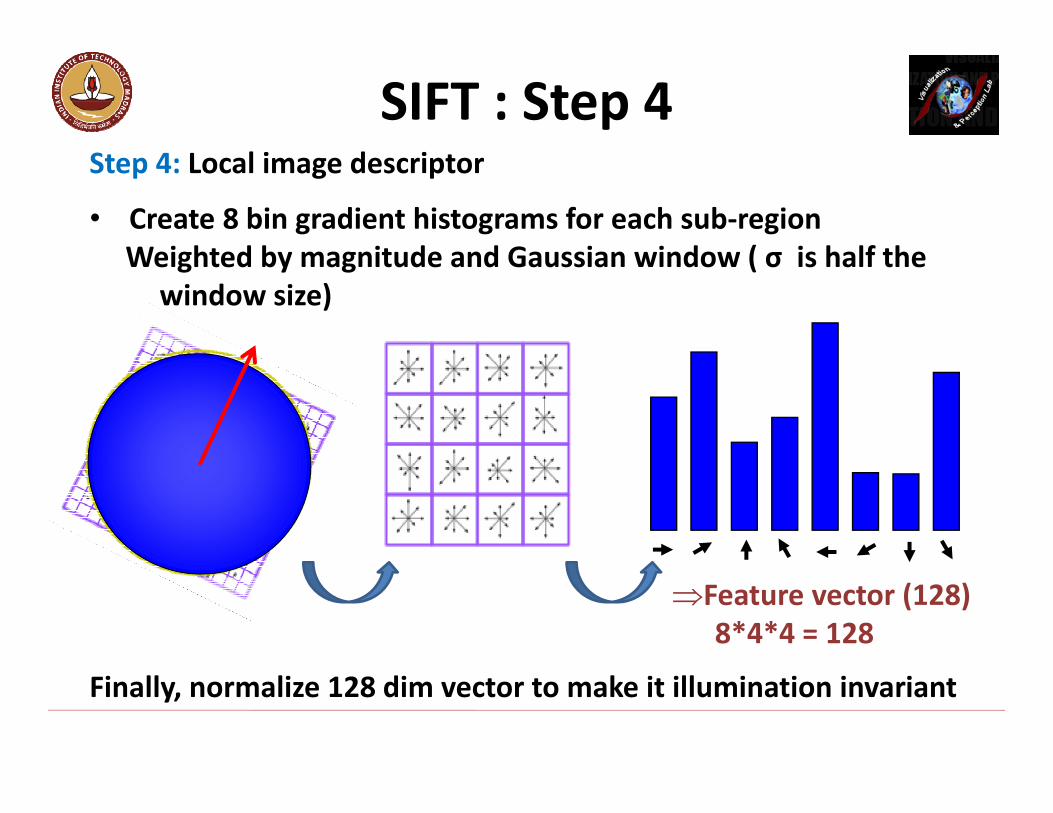
SIFT : Step 4Step 4: Local image descriptor

• Create 8 bin gradient histograms for each sub-regionWeighted by magnitude and Gaussian window ( σ is half the

window size)

Feature vector (128)8*4*4 = 128

Finally, normalize 128 dim vector to make it illumination invariant

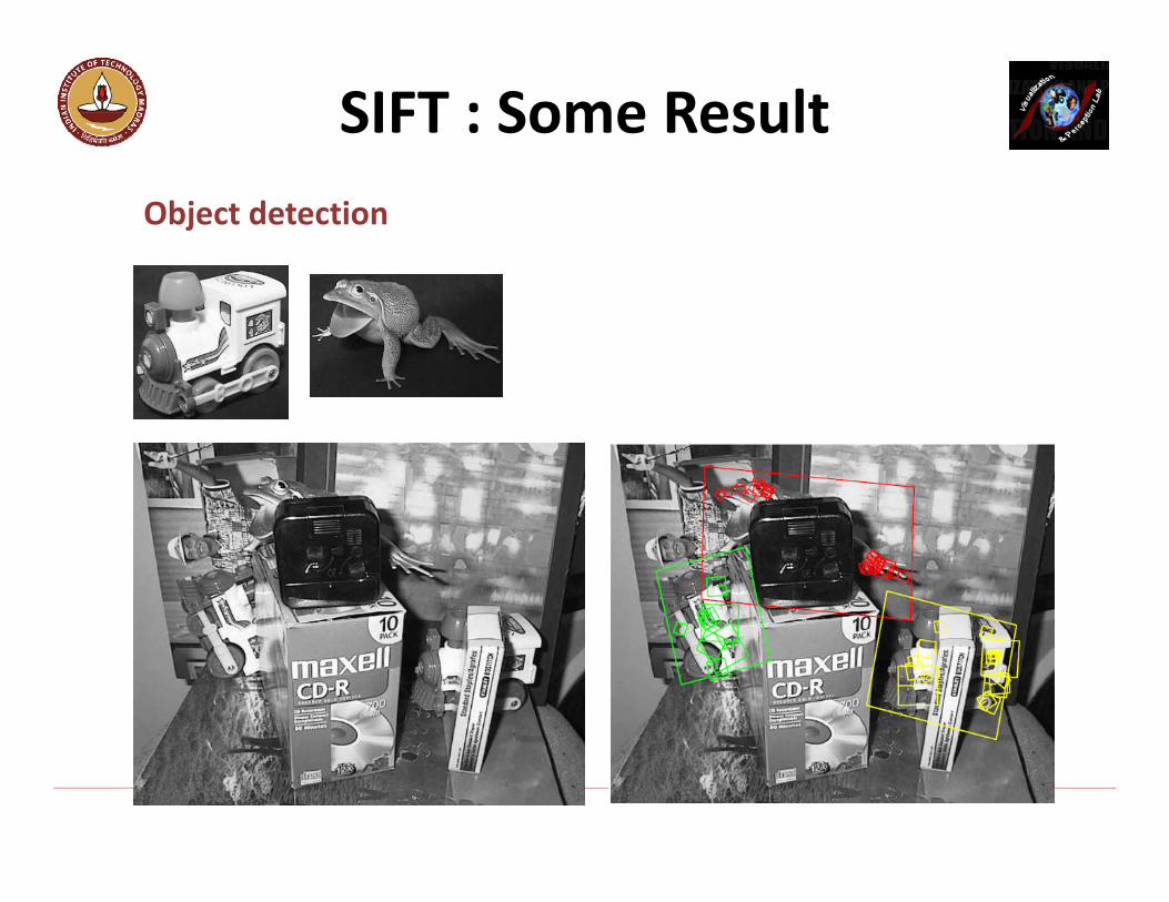
SIFT : Some ResultObject detection

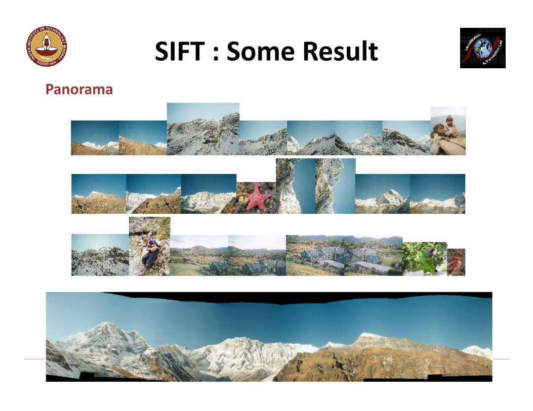
SIFT : Some ResultPanorama

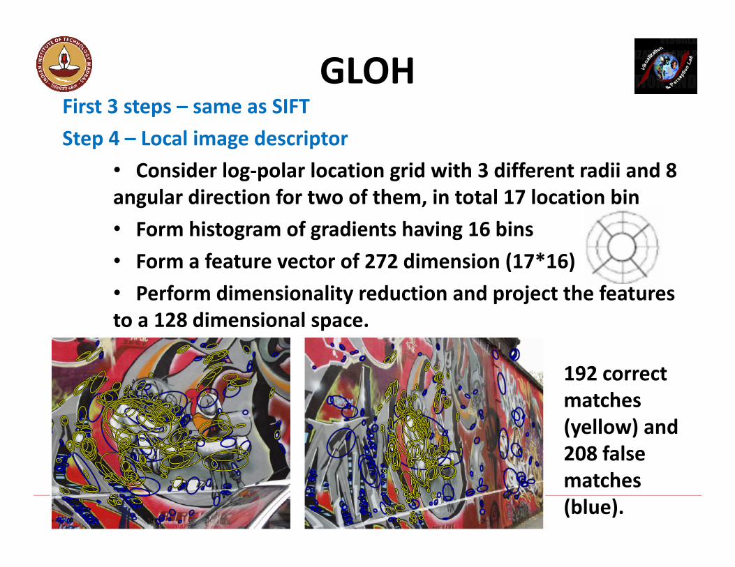
GLOHFirst 3 steps – same as SIFTStep 4 – Local image descriptor

• Consider log-polar location grid with 3 different radii and 8 angular direction for two of them, in total 17 location bin• Form histogram of gradients having 16 bins• Form a feature vector of 272 dimension (17*16)• Perform dimensionality reduction and project the features to a 128 dimensional space.

192 correct matches (yellow) and 208 false matches (blue).

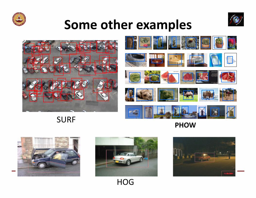
Some other examples

SURF

HOG

PHOW

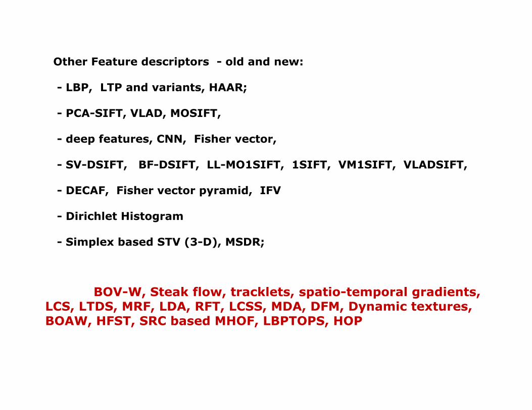
Other Feature descriptors - old and new:

- LBP, LTP and variants, HAAR;

- PCA-SIFT, VLAD, MOSIFT,

- deep features, CNN, Fisher vector,

- SV-DSIFT, BF-DSIFT, LL-MO1SIFT, 1SIFT, VM1SIFT, VLADSIFT,

- DECAF, Fisher vector pyramid, IFV

- Dirichlet Histogram

- Simplex based STV (3-D), MSDR;

BOV-W, Steak flow, tracklets, spatio-temporal gradients, LCS, LTDS, MRF, LDA, RFT, LCSS, MDA, DFM, Dynamic textures, BOAW, HFST, SRC based MHOF, LBPTOPS, HOP

Reference1. Kristen Grauman and Bastian Leibe, Visual Object Recognition, Synthesis Lectures

on Artificial Intelligence and Machine Learning, April 2011, Vol. 5, No. 2, Pages 1-181.

2. Beaudet, “Rotationally invariant image operators”, in International Joint Conference on Pattern Recognition, pp. 579-583., 1978.

3. Förstner, W. and Gülch, E., “A fast operator for detection and precise location of distinct points, corners and centers of circular features”, in ISPRS Inter commission Workshop’, pp. 281-305, 1987.

4. Harris, C. and Stephens, M., “A combined corner and edge detector”, in ‘Alvey Vision Conference’, pp. 147–151, 1988.

5. Lindeberg, T., ‘Scale-space theory: A basic tool for analyzing structures at different scales’, Journal of Applied Statistics 21(2), pp. 224–270, 1994.

6. Lowe, D., ‘Distinctive image features from scale-invariant keypoints’, International Journal of Computer Vision 60(2), pp. 91–110, 2004.

7. Mikolajczyk, K. and Schmid, C., ‘A performance evaluation of local descriptors’, IEEE Transactions on Pattern Analysis & Machine Intelligence 27(10), 31–37, 2005.

THANK YOU