local existence and exponential growth for a …
TRANSCRIPT

Advances in Differential Equations Volume 13, Numbers 11-12 (2008), 1051–1074
LOCAL EXISTENCE AND EXPONENTIAL GROWTH FORA SEMILINEAR DAMPED WAVE EQUATION WITH
DYNAMIC BOUNDARY CONDITIONS
Stephane GerbiLaboratoire de Mathematiques, Universite de Savoie
73376 Le Bourget du Lac, France
Belkacem Said-HouariLaboratoire de Mathematiques Appliquees, Universite Badji Mokhtar
B.P. 12 Annaba 23000, Algerie
(Submitted by: Juan Vazquez)
Abstract. In this paper we consider a multi-dimensional damped semi-linear wave equation with dynamic boundary conditions, related to theKelvin-Voigt damping. We firstly prove the local existence by using theFaedo-Galerkin approximations combined with a contraction mappingtheorem. Secondly, the exponential growth of the energy and the Lp
norm of the solution is presented.
1. Introduction
In this paper we consider the following semilinear damped wave equationwith dynamic boundary conditions:
utt −∆u− α∆ut = |u|p−2u, x ∈ Ω, t > 0u(x, t) = 0, x ∈ Γ0, t > 0
utt(x, t) = −[∂u∂ν
(x, t) +α∂ut∂ν
(x, t) + r|ut|m−2ut(x, t)]
x ∈ Γ1, t > 0u(x, 0) = u0(x), ut(x, 0) = u1(x) x ∈ Ω,
(1.1)where u = u(x, t), t ≥ 0, x ∈ Ω, ∆ denotes the Laplacian operator withrespect to the x variable, Ω is a regular and bounded domain of RN (N ≥ 1),∂Ω = Γ0 ∪ Γ1, mes(Γ0) > 0, Γ0∩Γ1 = ∅, ∂∂ν denotes the unit outer normalderivative, m ≥ 2, a, α and r are positive constants, p > 2 and u0, u1 aregiven functions.
Accepted for publication: July 2008.AMS Subject Classifications: 35L45, 35L70, 35B40.
1051

1052 Stephane Gerbi and Belkacem Said-Houari
From the mathematical point of view, these problems do not neglect ac-celeration terms on the boundary. Such types of boundary conditions areusually called dynamic boundary conditions. They are not only importantfrom the theoretical point of view but also arise in several physical appli-cations. In one space dimension, the problem (1.1) can model the dynamicevolution of a viscoelastic rod that is fixed at one end and has a tip mass at-tached to its free end. The dynamic boundary conditions represent Newton’slaw for the attached mass (see [5, 2, 11] for more details). In two-dimensionalspace, as showed in [26] and in the references therein, these boundary con-ditions arise when we consider the transverse motion of a flexible membraneΩ whose boundary may be affected by the vibrations only in a region. Alsosome dynamic boundary conditions as in problem (1.1) appear when we as-sume that Ω is an exterior domain of R3 in which homogeneous fluid is at restexcept for sound waves. Each point of the boundary is subjected to smallnormal displacements into the obstacle (see [3] for more details). This typeof dynamic boundary conditions are known as acoustic boundary conditions.
In the one-dimensional case and for r = 0, that is, in the absence ofboundary damping, this problem has been considered by Grobbelaar-VanDalsen [16]. By using the theory of B-evolutions and the theory of frac-tional powers developed in [27, 28], the author showed that the partial dif-ferential equations in the problem (1.1) give rise to an analytic semigroupin an appropriate functional space. As a consequence, the existence and theuniqueness of solutions was obtained. In the case where r 6= 0 and m = 2,Pellicer and Sola-Morales [25] considered the one-dimensional problem as analternative model for the classical spring-mass damper system, and by usingthe dominant eigenvalues method, they proved that for small values of theparameter a the partial differential equations in the problem (1.1) have theclassical second-order differential equation
m1u′′(t) + d1u
′(t) + k1u(t) = 0,
as a limit where the parameter m1, d1 and k1 are determined from the valuesof the spring-mass damper system. Thus, the asymptotic stability of themodel has been determined as a consequence of this limit. But they did notobtain any rate of convergence.
We recall that the presence of the strong damping term −∆ut in theproblem (1.1) makes the problem different from that considered in [15] andwidely studied in the literature [32, 29, 30, 14, 31] for instance. For thisreason fewer results were known for the wave equation with a strong dampingand many problems remained unsolved, especially the blow-up of solutionsin the presence of a strong damping and nonlinear damping at the same

Local existence and exponential growth 1053
time. Here we will give a partial answer to this question. That is to say,we will prove that the solution is unbounded and grows exponentially whentime goes to infinity.
Recently, Gazzola and Squassina [14] studied the global solution and thefinite time blow-up for a damped semilinear wave equation with Dirichletboundary conditions by a careful study of the stationary solutions and theirstability using the Nehari manifold and a mountain pass energy level of theinitial condition.
The main difficulty of the problem considered is related to the out ofthe ordinary boundary conditions defined on Γ1. Very little attention hasbeen paid to these types of boundary conditions. We mention only a fewparticular results in the one-dimensional space and for a linear damping in(m = 2) [18, 25, 12].
A problem related to (1.1) is the following:
utt −∆u+ g(ut) = f in Ω× (0, T )∂u
∂ν+K(u)utt + h(ut) = 0, on ∂Ω× (0, T )
u(x, 0) = u0(x) in Ωut(x, 0) = u1(x) in Ω,
where the boundary term h(ut) = |ut|ρ ut arises when one studies flows ofgas in a channel with porous walls. The term utt on the boundary appearsfrom the internal forces, and the nonlinearity K(u)utt on the boundary rep-resents the internal forces when the density of the medium depends on thedisplacement. This problem has been studied in [12, 13]. By using theFadeo-Galerkin approximations and a compactness argument they provedthe global existence and the exponential decay of the solution of the prob-lem.
We recall some results related to the interaction of an elastic medium withrigid mass. By using classical semigroup theory, Littman and Markus [21]established a uniqueness result for a particular Euler-Bernoulli beam rigidbody structure. They also proved asymptotic stability of the structure byusing the feedback boundary damping. In [22] the authors considered theEuler-Bernoulli beam equation which describes the dynamics of a clampedelastic beam in which one segment of the beam is made with viscoelastic ma-terial and the other of elastic material. By combining the frequency domainmethod with the multiplier technique, they proved exponential decay for thetransversal motion but not for the longitudinal motion of the model, whenthe Kelvin-Voigt damping is distributed only on a subinterval of the domain.

1054 Stephane Gerbi and Belkacem Said-Houari
In relation to this point, see also the work by Chen et al. [9] concerning theEuler-Bernoulli beam equation with the global or local Kelvin-Voigt damp-ing. Also models of vibrating strings with local viscoelasticity and Boltz-mann damping, instead of the Kelvin-Voigt one, were considered in [23] andan exponential energy decay rate was established. Recently, Grobbelaar-VanDalsen [17] considered an extensible thermo-elastic beam which is hangedat one end with rigid body attached to its free end, i.e., one-dimensionalhybrid thermoelastic structure, and showed that the method used in [24]is still valid to establish a uniform stabilization of the system. Concern-ing the controllability of the hybrid system we refer to the work by Castroand Zuazua[6], in which they considered flexible beams connected by pointmasses and the model takes account of the rotational inertia.
In this paper we consider the problem (1.1) where we have set for thesake of simplicity a = 1. Section 2 is devoted to the local existence anduniqueness of the solution of the problem (1.1). We will use a techniqueclose to the one used by Georgiev and Todorova in [15] and Vitillaro in[33, 34]: a Faedo-Galerkin approximation coupled to a fixed point theorem.
In section 3, we shall prove that the energy is unbounded when the initialdata are large enough. In fact, it will be proved that the Lp-norm of thesolutions grows as an exponential function. An essential ingredient of theproof is a lower bound in the Lp norm and the H1 seminorm of the solutionwhen the initial data are large enough, obtained by Vitillaro in [32]. Theother ingredient is the use of an auxiliary function L (which is a small pertur-bation of the energy) in order to obtain a linear differential inequality, thatwe integrate to finally prove that the energy is exponentially growing. Tothis end, we use Young’s inequality with suitable coefficient, interpolation,and Poincare’s inequalities.
Let us recall that the blow-up result in the case of a nonlinear damping(m 6= 2) is still an open problem.
2. Local existence
In this section we will prove the local existence and the uniqueness of thesolution of the problem (1.1). We will adapt the ideas used by Georgievand Todorova in [15], which consist in constructing approximations by theFaedo-Galerkin procedure in order to use the contraction mapping theorem.This method allows us to consider fewer restrictions on the initial data. Con-sequently, the same result can be established by using the Faedo-Galerkinapproximation method coupled with the potential well method [7].

Local existence and exponential growth 1055
2.1. Setup and notation. We present here some material that we shalluse in order to prove the local existence of the solution of problem (1.1).We denote H1
Γ0(Ω) =
u ∈ H1(Ω) : uΓ0 = 0
. By (., .) we denote the scalar
product in L2(Ω); i.e.,
(u, v)(t) =∫
Ωu(x, t)v(x, t)dx.
Also by ‖.‖q we mean the Lq(Ω) norm for 1 ≤ q ≤ ∞, and by ‖.‖q,Γ1 theLq(Γ1) norm.
Let T > 0 be a real number and X a Banach space endowed with norm‖.‖X . Lp(0, T ;X), 1 ≤ p <∞, denotes the space of functions f which are Lp
over (0, T ) with values in X, which are measurable with ‖f‖X ∈ Lp (0, T ).This space is a Banach space endowed with the norm
‖f‖Lp(0,T ;X) =(∫ T
0‖f‖pXdt
)1/p.
L∞ (0, T ;X) denotes the space of functions f : (0, T ) → X which are mea-surable with ‖f‖X ∈ L∞ (0, T ). This space is a Banach space endowed withthe norm
‖f‖L∞(0,T ;X) = ess sup0<t<T
‖f‖X .
We recall that if X and Y are two Banach spaces such that X → Y (con-tinuous embedding), then Lp (0, T ;X) → Lp (0, T ;Y ) , 1 ≤ p ≤ ∞. We willalso use the embedding (see [1, Theorem 5.8]):
H1Γ0
(Ω) → Lq(Γ1), 2 ≤ q ≤ q where q =
2(N−1)N−2 , if N ≥ 3
+∞, if N = 1, 2.
Let us denote V = H1Γ0
(Ω) ∩ Lm(Γ1).In this work, we cannot use “directly” the existence result of Georgiev and
Todorova [15] nor the results of Vitillaro [33, 34] because of the presence ofthe strong linear damping −∆ut and the dynamic boundary conditions onΓ1. Therefore, we have the next local existence theorem.
Theorem 2.1. Let 2 ≤ p ≤ q and max(2, qq+1−p) ≤ m ≤ q. Then given
u0 ∈ H1Γ0
(Ω) and u1 ∈ L2(Ω), there exist T > 0 and a unique solution u ofthe problem (1.1) on (0, T ) such that
u ∈ C([0, T ], H1
Γ0(Ω))∩C1
([0, T ], L2(Ω)
),
ut ∈ L2(0, T ;H1
Γ0(Ω))∩Lm
((0, T )× Γ1
).

1056 Stephane Gerbi and Belkacem Said-Houari
We will prove this theorem by using the Fadeo-Galerkin approximationsand the well-known contraction mapping theorem. In order to define thefunction for which a fixed point exists, we will consider first a related prob-lem. For u ∈ C
([0, T ], H1
Γ0(Ω))∩C1
([0, T ], L2(Ω)
)given, let us consider the
following problem:vtt −∆v − α∆vt = |u|p−2u, x ∈ Ω, t > 0v(x, t) = 0, x ∈ Γ0, t > 0
vtt(x, t) = −[∂v∂ν
(x, t) +α∂vt∂ν
(x, t) + r|vt|m−2vt(x, t)]
x ∈ Γ1, t > 0v(x, 0) = u0(x), vt(x, 0) = u1(x) x ∈ Ω.
(2.1)We have now to state the following existence result.
Lemma 2.1. Let 2 ≤ p ≤ q and max(2, qq+1−p) ≤ m ≤ q. Then given
u0 ∈ H1Γ0
(Ω) and u1 ∈ L2(Ω) there exist T > 0 and a unique solution v ofthe problem (2.1) on (0, T ) such that
v ∈ C([0, T ], H1
Γ0(Ω))∩C1
([0, T ], L2(Ω)
),
vt ∈ L2(0, T ;H1
Γ0(Ω))∩Lm
((0, T )× Γ1
)and satisfies the energy identity:
12[‖∇v‖22 + ‖vt‖22 + ‖vt‖22,Γ1
]ts
+ α
∫ t
s‖∇vt(τ)‖22dτ + r
∫ t
s‖vt(τ)‖mm,Γ1
dτ
=∫ t
s
∫Ω|u(τ)|p−2u(τ)vt(τ)dτdx
for 0 ≤ s ≤ t ≤ T .
In order to prove Lemma 2.1, we first study for any T > 0 and f ∈H1(0, T ;L2(Ω)) the following problem:
vtt −∆v − α∆vt = f(x, t), x ∈ Ω, t > 0v(x, t) = 0, x ∈ Γ0, t > 0
vtt(x, t) = −[∂v∂ν
(x, t) +α∂vt∂ν
(x, t) + r|vt|m−2vt(x, t)]
x ∈ Γ1, t > 0v(x, 0) = u0(x), vt(x, 0) = u1(x) x ∈ Ω.
(2.2)At this point, as done by Doronin et al. [13], we have to specify exactlywhat type of solutions of the problem (2.2) we expect.
Definition 2.1. A function v(x, t) such that
v ∈ L∞(0, T ;H1
Γ0(Ω)),
Local existence and exponential growth 1057
vt ∈ L2(0, T ;H1
Γ0(Ω))∩ Lm ((0, T )× Γ1) ,
vt ∈ L∞(0, T ;H1
Γ0(Ω))∩ L∞
(0, T ;L2(Γ1)
),
vtt ∈ L∞(0, T ;L2(Ω)
)∩ L∞
(0, T ;L2(Γ1)
),
v(x, 0) = u0(x),vt(x, 0) = u1(x),
is a generalized solution to the problem (2.2) if for any function ω ∈ H1Γ0
(Ω)∩Lm(Γ1) and ϕ ∈ C1(0, T ) with ϕ(T ) = 0, we have the following identity:∫ T
0(f, w)(t)ϕ(t)dt =
∫ T
0
[(vtt, w)(t) + (∇v,∇w)(t) + α(∇vt,∇w)(t)
]ϕ(t)dt
+∫ T
0ϕ(t)
∫Γ1
[vtt(t) + r|vt(t)|m−2vt(t)
]w dσ dt.
Lemma 2.2. Let 2 ≤ p ≤ q and 2 ≤ m ≤ q. Let u0 ∈ H2(Ω) ∩ V, u1 ∈H2(Ω) and f ∈ H1(0, T ;L2(Ω)), then for any T > 0, there exists a uniquegeneralized solution (in the sense of definition 2.1) v(t, x) of problem (2.2).
2.2. Proof of Lemma 2.2. To prove the above lemma, we will use theFaedo-Galerkin method, which consists in constructing approximations ofthe solution, then we obtain a priori estimates necessary to guarantee theconvergence of these approximations. Some difficulties appear deriving asecond-order estimate of vtt(0). To get rid of them, and inspired by theideas of Doronin and Larkin in [12] and Cavalcanti et al. [8], we introducethe following change of variables:
v(t, x) = v(t, x)− φ(t, x) with φ(t, x) = u0(x) + t u1(x).
Consequently, we have the following problem with the unknown v(t, x) andnull initial conditions:
vtt −∆v − α∆vt = f(x, t) + ∆φ+ α∆φt, x ∈ Ω, t > 0v(x, t) = 0, x ∈ Γ0, t > 0
vtt(x, t) = −[ ∂(v + φ)
∂ν(x, t) +
α∂(vt + φt)∂ν
(x, t)]
−(r|(vt + φt)|m−2(vt + φt)(x, t)
)x ∈ Γ1, t > 0
v(x, 0) = 0, vt(x, 0) = 0 x ∈ Ω.(2.3)
Remark 2.1. It is quite clear that if v is a solution of problem (2.3) on[0, T ], then v is a solution of problem (2.2) on [0, T ]. Moreover, writingthe problem in terms of v shows exactly the regularity needed on the initialconditions u0 and u1 to ensure the existence.

1058 Stephane Gerbi and Belkacem Said-Houari
Now we construct approximations of the solution v by the Faedo-Galerkinmethod as follows: For every n ≥ 1, let Wn = spanω1, . . . , ωn, whereωj(x)1≤j≤n is a basis in the space V . By using the Gram-Schmidt or-thogonalization process we can take ω = (ω1, . . . , ωn) to be orthonormal1 inL2(Ω) ∩ L2(Γ1). We define the approximations
vn(t) =n∑j=1
gjn(t)wj (2.4)
where vn(t) are solutions to the finite-dimensional Cauchy problem (writtenin normal form since ω is an orthonormal basis):∫
Ωvttn(t)wj dx+
∫Ω∇(vn + φ
)∇wj + α
∫Ω∇(vn + φ
)t∇wj dx
+∫
Γ1
(vttn(t) + r|(vn + φ)t|m−2(vn + φ)t
)wj dσ =
∫Ωfwj dx.
gjn(0) = g′jn(0) = 0, j = 1, . . . , n.
(2.5)
According to the Caratheodory theorem, see [10], the problem (2.5) has asolution (gjn(t))j=1,n ∈ H3(0, tn) defined on [0, tn). We need now to show:
• firstly that for all n ∈ N,, tn = T ;• secondly that these approximations converge to a solution of the
problem (2.3).To do this we need the two following a priori estimates: first-order a prioriestimates to prove the first point. But we will show that the presence of thenonlinear term |ut|m−2ut forces us to derive a second-order a priori estimateto pass to the limit in the nonlinear term. Indeed the key tool in our proofis the Aubin-Lions lemma which uses the compactness of the embeddingH
12 (Γ1) → L2(Γ1).
2.2.1. First order a priori estimates. Multiplying equation (2.5) by g′jn(t),integrating over (0, t) × Ω and using integration by parts we get: for everyn ≥ 1,
12[‖∇vn(t)‖22 + ‖vtn(t)‖22 + ‖vtn‖22,Γ1
]+∫ t
0
∫Ω∇φ∇vn dx
+ α
∫ t
0
∫Ω∇φt∇vtn dx+ α
∫ t
0‖∇vtn(s)‖22 ds (2.6)
1Unfortunately, the presence of the nonlinear boundary conditions excludes us fromusing the spatial basis of eigenfunctions of −∆ in H1
Γ0(Ω) as done in [14]

Local existence and exponential growth 1059
+ r
∫ t
0
∫Γ1
| (vn + φ)t |m−2(vn + φ)tvtn dσds =
∫ t
0
∫Ωf(t, x)vtn(s) dx ds.
By using Young’s inequality, there exists δ1 > 0 (in fact small enough) suchthat
α
∫ t
0
∫Ω∇φt∇vtndx ≤ δ1
∫ t
0
∫Ω|∇vtn|2dx+
14δ1
∫ t
0
∫Ω|∇φt|2dx (2.7)
and ∫ t
0
∫Ω∇φ∇vndx ≤ δ1
∫ t
0
∫Ω|∇vn|2dx+
14δ1
∫ t
0
∫Ω∇φ|2dx. (2.8)
By Young’s and Poincare’s inequalities, we can find C > 0, such that∫ t
0
∫Ωf(t, x)vtn(s)dxds ≤ C
∫ t
0
∫Ω
(f2 + |∇vtn(s)|2
)dxds. (2.9)
The last term in the left-hand side of equation (2.6) can be written as follows:∫ t
0
∫Γ1
| (vn + φ)t |m−2 (vn + φ)t vtndσds
=∫ t
0
∫Γ1
| (vn + φ)t |mdσds−
∫ t
0
∫Γ1
| (vn + φ)t |m−2 (vn + φ)t φtdσds.
Then Young’s inequality gives us, for δ2 > 0,∣∣∣ ∫ t
0
∫Γ1
| (vn + φ)t |m−2 (vn + φ)t φtdσds
∣∣∣ (2.10)
≤ δm2m
∫ t
0
∫Γ1
| (vn + φ)t |mdσds+
m− 1m
δ−m/(m−1)2
∫ t
0
∫Γ1
|φt|mdσds.
Consequently, using the inequalities (2.7), (2.8), (2.9) and (2.10) in equation(2.6), choosing δ1 and δ2 small enough, we may conclude that
12[‖∇vn(t)‖22 + ‖vtn(t)‖22 + ‖vtn(t)‖22,Γ1
](2.11)
+ α
∫ t
0‖∇vtn(s)‖22ds+ r
∫ t
0
∫Γ1
| (vn + φ)t |mdσds ≤ CT ,
where CT is a positive constant independent of n. Therefore, the last esti-mate (2.11) gives us, for all n ∈ N, tn = T , and
(vn)n∈N is bounded in L∞(0, T ;H1Γ0
(Ω)), (2.12)
(vtn)n∈N is bounded in (2.13)
L∞(0, T ;L2(Ω)) ∩ L2(0, T ;H1
Γ0(Ω))∩ L∞
(0, T ;L2(Γ1)
).

1060 Stephane Gerbi and Belkacem Said-Houari
Now, by using the following algebraic inequality:
(A+B)λ ≤ 2λ−1(Aλ +Bλ), A,B ≥ 0, λ ≥ 1, (2.14)
we can find c1, c2 > 0, such that∫ t
0
∫Γ1
|(vn + φ)t|mdσds ≥ c1
∫ t
0
∫Γ1
|vtn|mdσds− c2
∫ t
0
∫Γ1
|φt|mdσds.
(2.15)Then by the embedding H2(Ω) → Lm(Γ1) (2 ≤ m ≤ q), we conclude thatu1 ∈ Lm(Γ1). Therefore, from the inequalities (2.11) and (2.15), there existsC ′T > 0 such that ∫ t
0
∫Γ1
|vtn|mdσds ≤ C ′T .
Consequently,vtn is bounded in Lm((0, T )× Γ1). (2.16)
2.2.2. Second order a priori estimate. In order to obtain a second a prioriestimate, we will first estimate ‖vttn(0)‖22 and ‖vttn(0)‖22,Γ1
. For this purpose,considering wj = vttn(0) and t = 0 in the equation (2.5), we get
‖vttn(0)‖22 + ‖vttn(0)‖22,Γ1+∫
Ω∇φ(0)∇vttn(0)dx (2.17)
+ α
∫Ω∇φt(0)∇vttn(0)dx+ r
∫Γ1
|φt(0)|m−2φt(0)vttn(0)dσds
=∫
Ωf(0, x)vttn(0)dxds.
Since the following equalities hold:
φ(0) = u0, φt(0) = u1,∫Ω∇φt(0)∇vttn(0) = −
∫Ω
∆φt(0)vttn(0) +∫
Γ1
φt∂vttn∂ν
dσ,
as f ∈ H1(0, T ;L2(Ω)) and u0, u1 ∈ H2(Ω), by using Young’s inequalityand the embedding H2(Ω) → Lm(Γ1), we conclude that there exists C > 0independent of n such that
‖vttn(0)‖22 + ‖vttn(0)‖22,Γ1≤ C. (2.18)
Differentiating equation (2.5) with respect to t, multiplying the result byg′′jn(t) and summing over j, we get
12d
dt
[‖∇vtn(t)‖22 + ‖vttn(t)‖22 + ‖vttn(t)‖22,Γ1
]+∫
Ω∇φt∇vttndx (2.19)

Local existence and exponential growth 1061
+ α‖∇vttn(s)‖22 + r(m− 1)∫
Γ1
|(vn + φ)t|m−2(vn + φ)ttvttndσ
=∫
Ωft(t, x)vttn(s)dxds.
Since φtt = 0, the last term in the left-hand side of equation (2.19) can bewritten as follows:∫
Γ1
|(vn + φ)t|m−2(vn + φ)ttvttndσ =∫
Γ1
|(vn + φ)t|m−2(vttn + φtt)2dσ.
But we have ∫Γ1
|(vn + φ)t|m−2(vttn + φtt)2dσ
=4m2
∫Γ1
( ∂∂t
(|vtn(t) + φt|
m−22 (vtn(t) + φt
))2dσ.
Now, integrating equation (2.19) over (0, t), using the inequality (2.18) andYoung’s and Poincare’s inequalities (as in (2.10)), there exists CT > 0 suchthat
12
[‖∇vtn(t)‖22 + ‖vttn(t)‖22 + ‖vttn(t)‖22,Γ1
]+α
∫ t
0‖∇vttn(s)‖22
+4r (m− 1)
m2
∫Γ1
( ∂∂t
(|vtn(t) + φt|
m−22 (vtn(t) + φt
))2dσ ≤ CT .
Consequently, we deduce the following results:
(vttn(t))n∈N is bounded in L∞(0, T ;L2(Ω)
),
(vttn(t))n∈N is bounded in L∞(0, T ;L2 (Γ1)
),
(vtn(t))n∈N is bounded in L∞(0, T ;H1
Γ0(Ω)).
(2.20)
From (2.12), (2.13), (2.16), and (2.20), we have (vn)n∈N bounded in L∞(0, T ;H1
Γ0(Ω)). Then (vn)n∈N is bounded in L2(0, T ;H1
Γ0(Ω)). Since (vtn)n∈N is
bounded in L∞(0, T ;L2(Ω)), (vtn)n∈N is bounded in L2(0, T ; L2(Ω)). Con-sequently, (vn)n∈N is bounded in H1(0, T ;H1(Ω)). Since the embeddingH1(0, T ;H1(Ω)
)→ L2
(0, T ;L2(Ω)
)is compact, by using the Aubin-Lions
theorem, we can extract a subsequence (vµ)µ∈N of (vn)n∈N such that vµ →v strongly in L2
(0, T ;L2(Ω)
). Therefore, vµ → v strongly and almost every-
where on (0, T )×Ω. Following [19, Lemme 3.1], we get |vµ|p−2vµ → |v|p−2vstrongly and almost everywhere on (0, T ) × Ω. On the other hand, we al-ready have proved in the preceding section that (vtn)n∈N is bounded in
1062 Stephane Gerbi and Belkacem Said-Houari
L∞(0, T ;L2 (Γ1)
). From (2.12) and (2.20), since
‖vn(t)‖H
12 (Γ1)
≤ C‖∇vn(t)‖2 and ‖vtn(t)‖H
12 (Γ1)
≤ C‖∇vtn(t)‖2
we deduce that
(vn)n∈N is bounded in L2(0, T ;H
12 (Γ1)
),
(vtn)n∈N is bounded in L2(0, T ;H
12 (Γ1)
),
(vttn)n∈N is bounded in L2(0, T ;L2(Γ1)
).
Since the embedding H12 (Γ1) → L2(Γ1) is compact, again by using the
Aubin-Lions theorem, we conclude that we can extract a subsequence alsodenoted (vµ)µ∈N of (vn)n∈N such that
vtµ → vt strongly in L2(0, T ;L2(Γ1)
). (2.21)
Therefore, from (2.16), we obtain that
|vtµ|m−2vtµ χ weakly in Lm′((0, T )× Γ1) .
It suffices to prove now that χ = |vt|m−2vt. Clearly, from (2.21) we get
|vtµ|m−2vtµ → |vt|m−2vt strongly and a.e on (0, T )× Γ1.
Again, by using Lions’s lemma, [19, Lemme 1.3], we obtain χ = |vt|m−2vt.The proof now can be completed arguing as in [19, Theoreme 3.1].
2.2.3. Uniqueness. Let v, w be two solutions of the problem (2.2) which sharethe same initial data. Let us denote z = v − w. It is straightforward to seethat z satisfies
‖∇z‖22 + ‖∇zt‖22 + ‖zt‖22,Γ1+ 2α
∫ t
0‖∇z‖22ds (2.22)
+ 2r∫ t
0
∫Γ1
[|vt(s)|m−2vt(s)− |wt(s)|m−2wt(s)
](vt(s)− wt(s))dsdσ = 0.
By using the algebraic inequality
∀m ≥ 2, ∃ c > 0, ∀ a, b ∈ R,[|a|m−2a− |b|m−2b
](a− b) ≥ c|a− b|m (2.23)
equation (2.22) implies
‖zt‖22 + ‖∇z‖22 + ‖zt‖22,Γ1+ 2α
∫ t
0‖∇zt‖22ds
+ c
∫ t
0
∫Γ1
|vt (s)− wt(s)|mdsdσ ≤ 0
which implies z = 0. This finishes the proof of Lemma 2.2.

Local existence and exponential growth 1063
2.3. Proof of Lemma 2.1. We first approximate u ∈ C([0, T ], H1
Γ0(Ω))∩
C1([0, T ], L2(Ω)
)endowed with the standard norm
‖u‖ = maxt∈[0,T ]
‖ut(t)‖2 + ‖u(t)‖H1(Ω),
by a sequence (uk)k∈N ⊂ C∞([0, T ]×Ω) by standard convolution arguments(see [4]). It is clear that f
(uk)
= |uk|p−2uk ∈ H1(0, T ;L2(Ω)
). This type
of approximation has been already used by Vitillaro in [33, 34]. Next, weapproximate the initial data u1 ∈ L2(Ω) by a sequence (uk1)k∈N ⊂ C∞0 (Ω).Finally, since the space H2(Ω) ∩ V ∩H1
Γ0(Ω) is dense in H1
Γ0(Ω) for the H1
norm, we approximate u0 ∈ H1Γ0
(Ω) by a sequence (uk0)k∈N ⊂ H2(Ω) ∩ V ∩H1
Γ0(Ω).
We consider now the set of the following problems:
vktt −∆vk − α∆vkt = |uk|p−2uk, x ∈ Ω, t > 0vk(x, t) = 0, x ∈ Γ0, t > 0
vktt(x, t) = −[∂vk∂ν
(x, t) +α∂vkt∂ν
(x, t) + r|vkt |m−2vkt (x, t)]
x ∈ Γ1, t > 0
vk(x, 0) = uk0, vkt (x, 0) = uk1 x ∈ Ω.
(2.24)Since every hypothesis of Lemma 2.2 is satisfied, we can find a sequence ofunique solutions (vk)k∈N of the problem (2.24). Our goal now is to showthat (vk, vkt )k∈N is a Cauchy sequence in the space
YT =
(v, vt) : v ∈ C([0, T ] , H1
Γ0(Ω))∩ C1
([0, T ] , L2(Ω)
),
vt ∈ L2(0, T ;H1
Γ0(Ω))∩ Lm ((0, T )× Γ1)
endowed with the norm
‖(v, vt)‖2YT = max0≤t≤T
[‖vt‖22 + ‖∇v‖22
]+‖vt‖2
Lm(
(0,T )×Γ1
) +∫ t
0‖∇vt(s)‖22 ds.
For this purpose, we set U = uk − uk′ , V = vk − vk′ . It is straightforwardto see that V satisfies
Vtt −∆V −α∆Vt = |uk|p−2uk − |uk′ |p−2uk′
x ∈ Ω, t > 0V (x, t) = 0 x ∈ Γ0, t > 0
Vtt(x, t) = −[∂V∂ν
(x, t) +α∂Vt∂ν
(x, t)]
−r(|vkt |m−2vkt (x, t)− |vk′t |m−2vk
′t (x, t)
)x ∈ Γ1, t > 0
V (x, 0) = uk0 − uk′
0 , Vt(x, 0) = uk1 − uk′
1 x ∈ Ω.

1064 Stephane Gerbi and Belkacem Said-Houari
We multiply the above differential equations by Vt, we integrate over (0, t)×Ωand we use integration by parts to obtain
12
(‖Vt‖22 + ‖∇V ‖22 + ‖Vt‖22,Γ1
)+ α
∫ t
0‖∇Vt‖22 ds
+ r
∫ t
0
∫Γ1
(|vkt |m−2vkt − |vk
′t |m−2vk
′t
)(vkt − vk
′t
)dσds
=12(‖Vt(0)‖22 + ‖∇V (0)‖22 + ‖Vt(0)‖22,Γ1
)+
∫ t
0
∫Ω
(|uk|p−2uk − |uk′ |p−2uk
′)(
vkt − vk′t
)dxdτ, ∀t ∈ (0, T ) .
By using the algebraic inequality (2.23), we get
12(‖Vt‖22 + ‖∇V ‖22 + ‖Vt‖22,Γ1
)+ α
∫ t
0‖∇Vt‖22ds+ c1‖Vt‖mm,Γ1
≤ 12(‖Vt(0)‖22 + ‖∇V (0)‖22 + ‖Vt(0)‖22,Γ1
)+∫ t
0
∫Ω
(|uk|p−2uk − |uk′ |p−2uk
′)(
vkt − vk′t
)dxdτ, ∀t ∈ (0, T ) .
In order to find a majorant of the term∫ t
0
∫Ω
(|uk|p−2uk − |uk′ |p−2uk
′)(
vkt − vk′t
)dxdτ, ∀t ∈ (0, T ) ,
in the previous inequality, we use the result of Georgiev and Todorova [15](specifically their equations (2.5) and (2.6) in proposition 2.1). The hypoth-esis on p allows us to use exactly the same argument. Thus by applyingYoung’s inequality and the Gronwall inequality, there exists C dependingonly on Ω and p such that
‖V ‖YT ≤ C(‖Vt(0)‖22 + ‖∇V (0)‖22 + ‖Vt(0)‖22,Γ1
)+ CT‖U‖YT .
Let us now remark that from the notation used above, we have V (0) =uk0 − uk
′0 , Vt(0) = uk1 − uk
′1 , and U = uk − uk
′. Thus, since (uk0)k∈N is a
converging sequence in H1Γ0
(Ω), (uk1)k∈N is a converging sequence in L2(Ω)and (uk)k∈N is a converging sequence in C([0, T ], H1
Γ0(Ω))∩C1([0, T ], L2(Ω))
(thus in YT also), we conclude that (vk, vkt )k∈N is a Cauchy sequence in YT .Thus, (vk, vkt ) converges to a limit (v, vt) ∈ YT . Now by the same procedureused by Georgiev and Todorova in [15], we prove that this limit is a weaksolution of the problem (2.1). This completes the proof of Lemma 2.1.

Local existence and exponential growth 1065
2.4. Proof of theorem 2.1. In order to prove theorem 2.1, we use thecontraction mapping theorem.
For T > 0, let us define the convex closed subset of YTXT = (v, vt) ∈ YT : v(0) = u0, vt(0) = u1 .
Let us denote BR (XT ) = v ∈ XT : ‖v‖YT ≤ R . Then, Lemma 2.1 impliesthat, for any u ∈ XT , we may define v = Φ (u) to be the unique solution of(2.1) corresponding to u. Our goal now is to show that, for a suitable T > 0,Φ is a contractive map satisfying Φ (BR(XT )) ⊂ BR(XT ).
Let u ∈ BR(XT ) and v = Φ (u). Then, for all t ∈ [0, T ], we have
‖vt‖22 + ‖∇v‖22 + ‖vt‖22,Γ1+ 2
∫ t
0‖vt‖mm,Γ1
ds+ 2α∫ t
0‖∇vt‖22 ds (2.25)
= ‖u1‖22 + ‖∇u0‖22 + ‖u1‖22,Γ1+ 2
∫ t
0
∫Ω|u (τ) |p−2u (τ) vt (τ) dx dτ.
Using the Holder inequality, we can control the last term in the right-handside of the inequality (2.25) as follows:∫ t
0
∫Ω|u (τ) |p−2u (τ) vt (τ) dxdτ
≤∫ t
0‖u (τ) ‖p−1
2N/(N−2)‖vt (τ) ‖2N/(
3N−Np+2(p−1))dτ.
Since p ≤ 2NN−2 , we have
2N(3N −Np+ 2(p− 1)
) ≤ 2NN − 2
.
Thus, by Young’s and Sobolev’s inequalities, we conclude that, for all δ > 0,there exists C(δ) > 0, such that for all t ∈ (0, T ) ,∫ t
0
∫Ω|u (τ) |p−2u (τ) vt (τ) dxdτ ≤ C(δ)tR2(p−1) + δ
∫ t
0‖∇vt (τ) ‖22dτ.
Inserting the last estimate in the inequality (2.25) and choosing δ smallenough in order to counter-balance the last term of the left-hand side of theinequality (2.25) we get
‖v‖2YT ≤12R2 + CTR2(p−1).
Thus, for T sufficiently small, we have ‖v‖YT ≤ R. This shows that v ∈BR (XT ).
Next, we have to verify that Φ is a contraction. To this end, we setU = u − u and V = v − v, where v = Φ(u) and v = Φ(u) are the solutions

1066 Stephane Gerbi and Belkacem Said-Houari
of problem (2.1) corresponding respectively to u and u. Consequently, wehave
Vtt −∆V −α∆Vt = |u|p−2u− |u|p−2u x ∈ Ω, t > 0V (x, t) = 0 x ∈ Γ0, t > 0
Vtt(x, t) = −[∂V∂ν
(x, t) +α∂Vt∂ν
(x, t)]
−r(|vt|m−2vt(x, t)− |vt|m−2vt(x, t)
)x ∈ Γ1, t > 0
V (x, 0) = 0, Vt(x, 0) = 0 x ∈ Ω.
(2.26)
By multiplying the differential equation (2.26) by Vt and integrating over(0, t)× Ω, we get
12
(‖Vt‖22 + ‖∇V ‖22 + ‖Vt‖22,Γ1
)+ α
∫ t
0‖∇Vt‖22ds
+r∫ t
0
∫Γ1
(|vt|m−2vt − |vt|m−2vt
)(vt − vt)dσds
=∫ t
0
∫Ω
(|u|p−2u− |u|p−2u
)(vt − vt)dxdτ,∀t ∈ (0, T ).
Again, by using the algebraic inequality (2.23), we have
12(‖Vt‖22 + ‖∇V ‖22 + ‖Vt‖22,Γ1
)+ α
∫ t
0‖∇Vt‖22ds+ c1‖Vt‖mm,Γ1
≤∫ t
0
∫Ω
(|u|p−2u− |u|p−2u
)(vt − vt)dxdτ,∀t ∈ (0, T ) .
(2.27)
To estimate the term in the right-hand side of the inequality (2.27), let usdenote
I(t) :=∫ t
0
∫Ω
(|u|p−2u− |u|p−2u
)(vt − vt) dx dτ.
Using the algebraic inequality∣∣|u|p−2u− |u|p−2u∣∣ ≤ cp|u− u| (|u|p−2 + |u|p−2
),
which holds for any u, u ∈ R, where cp is a positive constant depending onlyon p, we find
I(t) ≤ cp∫ T
0
∫Ω|u− u|
(|u|p−2 + |u|p−2
)|Vt| dx dτ.
Following the same argument as Vitillaro in [34, equation 77], choosing p <r0 < q such that
q
q − p+ 1<
r0
r0 − p+ 1< m,
Local existence and exponential growth 1067
let s > 1 such that1m
+1r0
+1s
= 1.
Using Holder’s inequality we obtain
I(t) ≤ cp∫ T
0(‖u− u‖r0‖Vt‖m) .
(∫Ω
(|u|p−2 + |u|p−2
)s)1/s
. (2.28)
Therefore, the algebraic inequality (2.14) gives us(∫Ω
(|u|p−2 + |u|p−2
)s)1/s
≤ 2s−1(‖u‖(p−2)s
(p−2)s + ‖u‖(p−2)s(p−2)s
)1/s.
But since
(A+B)β ≤ Aβ +Bβ, ∀A, B ≥ 0 and 0 < β < 1
we get(∫Ω
(|u|p−2 + |u|p−2
)s)1/s
≤ 2s−1(‖u‖(p−2)
(p−2)s + ‖u‖(p−2)(p−2)s
). (2.29)
Consequently, inserting the inequality (2.28) in (2.29) and using Poincare’sinequality, we obtain
I(t) ≤ c2Rp−2
∫ T
0‖u− u‖r0‖∇Vt‖2ds.
Applying Holder’s inequality in time, we finally get
I(t) ≤ c2Rp−2T 1/2‖u− u‖L∞(0,T ;Lr0 (Ω))
(∫ T
0‖∇Vt‖22
)1/2
≤ c2
2Rp−2T 1/2
[‖u− u‖2L∞(0,T ;Lr0 (Ω)) +
∫ T
0‖∇Vt‖22
].
(2.30)
Lastly, by choosing T small enough in order to have α − c22 R
p−2T 1/2 > 0,we conclude by inserting the estimate (2.30) in the estimate (2.27) that
12(‖Vt‖22 + ‖∇V ‖22 + ‖Vt‖22,Γ1
)+ α
∫ t
0‖∇Vt‖22ds+ c1‖Vt‖mm,Γ1
≤ c2
2Rp−2T 1/2‖u− u‖2L∞(0,T ;Lr0 (Ω)).
(2.31)
Since r0 < q, using the embedding L∞(0, T ;H1
Γ0(Ω))→ L∞ (0, T ;Lr0(Ω))
in the estimate (2.31), we finally have
‖V ‖2YT ≤ c3Rp−2T 1/2‖U‖2YT . (2.32)
1068 Stephane Gerbi and Belkacem Said-Houari
By choosing T small enough in order to have c3Rp−2T 1/2 < 1, estimate
(2.32) shows that Φ is a contraction. Consequently the contraction mappingtheorem guarantees the existence of a unique v satisfying v = Φ(v). Theproof of theorem 2.1 is now completed.
Remark 2.2. To prove the existence and uniqueness of the solution to themore general problem
utt −∆u− α∆ut = f(u), x ∈ Ω, t > 0u(x, t) = 0, x ∈ Γ0, t > 0
utt(x, t) = −[∂u∂ν
(x, t) +α∂ut∂ν
(x, t) + g(ut)]
x ∈ Γ1, t > 0
u(x, 0) = u0(x), ut(x, 0) = u1(x) x ∈ Ω,
we can use the same method, provided that the functions f and g satisfyrespectively the conditions (H3) − (H7) and (H8) − (H9) of the paper ofCalvacanti et al. [8].
3. Exponential growth
In this section we consider the problem (1.1) and we will prove that whenthe initial data are large enough (in the energy point of view), the energygrows exponentially and thus the Lp norm does also.
In order to state and prove the result, we introduce the following notation.Let B be the best constant of the embedding H1
0 (Ω) → Lp(Ω) defined by
B−1 = inf‖∇u‖2 : u ∈ H1
0 (Ω), ‖u‖p = 1.
We also define the energy functional
E(u(t)) = E(t) =12‖∇u‖22 −
1p‖u‖pp +
12‖ut‖22 +
12‖ut‖22,Γ1
. (3.1)
Finally we define the following constant which will play an important rolein the proof of our result:
α1 = B−p/(p−2) and d = (12 −
1p)α2
1. (3.2)
In order to obtain the exponential growth of the energy, we will use thefollowing lemma (see Vitillaro [32], for the proof).
Lemma 3.1. Let u be a classical solution of (1.1). Assume that E(0) < dand ‖∇u0‖2 > α1. Then there exists a constant α2 > α1 such that
‖∇u(., t)‖2 ≥ α2, ∀t ≥ 0, (3.3)
and‖u‖p ≥ Bα2, ∀t ≥ 0. (3.4)
Local existence and exponential growth 1069
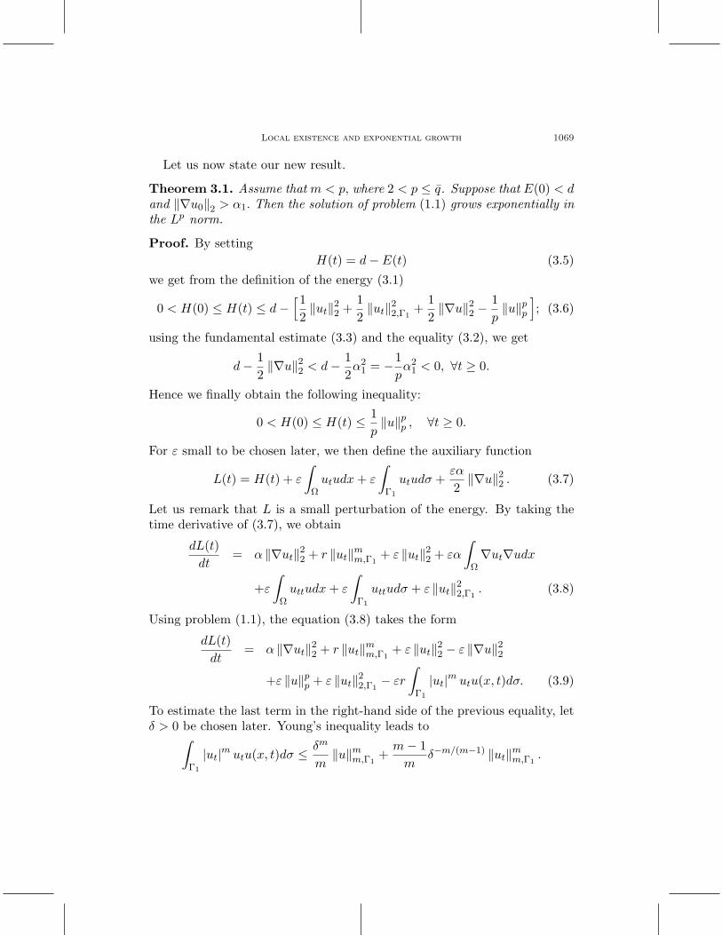
Let us now state our new result.
Theorem 3.1. Assume that m < p, where 2 < p ≤ q. Suppose that E(0) < dand ‖∇u0‖2 > α1. Then the solution of problem (1.1) grows exponentially inthe Lp norm.
Proof. By settingH(t) = d− E(t) (3.5)
we get from the definition of the energy (3.1)
0 < H(0) ≤ H(t) ≤ d−[1
2‖ut‖22 +
12‖ut‖22,Γ1
+12‖∇u‖22 −
1p‖u‖pp
]; (3.6)
using the fundamental estimate (3.3) and the equality (3.2), we get
d− 12‖∇u‖22 < d− 1
2α2
1 = −1pα2
1 < 0, ∀t ≥ 0.
Hence we finally obtain the following inequality:
0 < H(0) ≤ H(t) ≤ 1p‖u‖pp , ∀t ≥ 0.
For ε small to be chosen later, we then define the auxiliary function
L(t) = H(t) + ε
∫Ωutudx+ ε
∫Γ1
utudσ +εα
2‖∇u‖22 . (3.7)
Let us remark that L is a small perturbation of the energy. By taking thetime derivative of (3.7), we obtain
dL(t)dt
= α ‖∇ut‖22 + r ‖ut‖mm,Γ1+ ε ‖ut‖22 + εα
∫Ω∇ut∇udx
+ε∫
Ωuttudx+ ε
∫Γ1
uttudσ + ε ‖ut‖22,Γ1. (3.8)
Using problem (1.1), the equation (3.8) takes the form
dL(t)dt
= α ‖∇ut‖22 + r ‖ut‖mm,Γ1+ ε ‖ut‖22 − ε ‖∇u‖
22
+ε ‖u‖pp + ε ‖ut‖22,Γ1− εr
∫Γ1
|ut|m utu(x, t)dσ. (3.9)
To estimate the last term in the right-hand side of the previous equality, letδ > 0 be chosen later. Young’s inequality leads to∫
Γ1
|ut|m utu(x, t)dσ ≤ δm
m‖u‖mm,Γ1
+m− 1m
δ−m/(m−1) ‖ut‖mm,Γ1.
1070 Stephane Gerbi and Belkacem Said-Houari
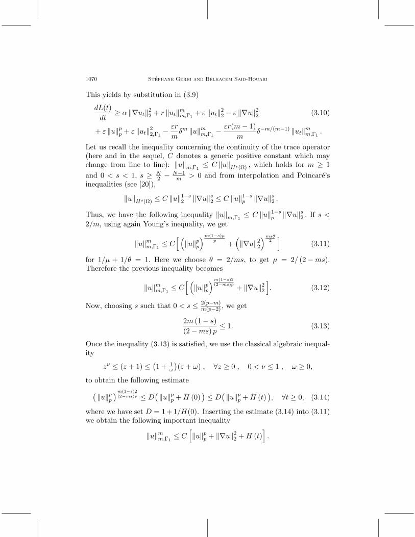
This yields by substitution in (3.9)
dL(t)dt≥ α ‖∇ut‖22 + r ‖ut‖mm,Γ1
+ ε ‖ut‖22 − ε ‖∇u‖22 (3.10)
+ ε ‖u‖pp + ε ‖ut‖22,Γ1− εr
mδm ‖u‖mm,Γ1
− εr(m− 1)m
δ−m/(m−1) ‖ut‖mm,Γ1.
Let us recall the inequality concerning the continuity of the trace operator(here and in the sequel, C denotes a generic positive constant which maychange from line to line): ‖u‖m,Γ1
≤ C ‖u‖Hs(Ω) , which holds for m ≥ 1and 0 < s < 1, s ≥ N
2 −N−1m > 0 and from interpolation and Poincare’s
inequalities (see [20]),
‖u‖Hs(Ω) ≤ C ‖u‖1−s2 ‖∇u‖s2 ≤ C ‖u‖
1−sp ‖∇u‖s2 .
Thus, we have the following inequality ‖u‖m,Γ1≤ C ‖u‖1−sp ‖∇u‖s2 . If s <
2/m, using again Young’s inequality, we get
‖u‖mm,Γ1≤ C
[ (‖u‖pp
)m(1−s)µp +
(‖∇u‖22
)msθ2]
(3.11)
for 1/µ + 1/θ = 1. Here we choose θ = 2/ms, to get µ = 2/ (2−ms).Therefore the previous inequality becomes
‖u‖mm,Γ1≤ C
[ (‖u‖pp
)m(1−s)2(2−ms)p + ‖∇u‖22
]. (3.12)
Now, choosing s such that 0 < s ≤ 2(p−m)m(p−2) , we get
2m (1− s)(2−ms) p
≤ 1. (3.13)
Once the inequality (3.13) is satisfied, we use the classical algebraic inequal-ity
zν ≤ (z + 1) ≤(1 + 1
ω
)(z + ω) , ∀z ≥ 0 , 0 < ν ≤ 1 , ω ≥ 0,
to obtain the following estimate(‖u‖pp
)m(1−s)2(2−ms)p ≤ D
(‖u‖pp +H (0)
)≤ D
(‖u‖pp +H (t)
), ∀t ≥ 0, (3.14)
where we have set D = 1 + 1/H(0). Inserting the estimate (3.14) into (3.11)we obtain the following important inequality
‖u‖mm,Γ1≤ C
[‖u‖pp + ‖∇u‖22 +H (t)
].
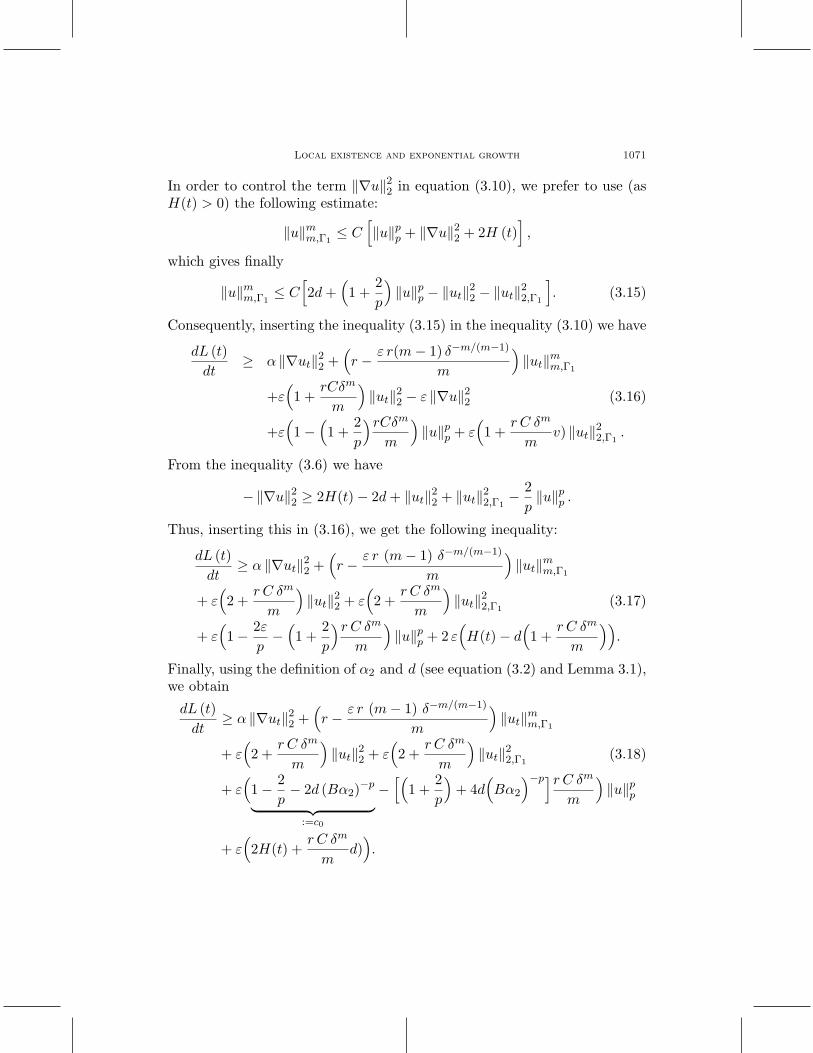
Local existence and exponential growth 1071
In order to control the term ‖∇u‖22 in equation (3.10), we prefer to use (asH(t) > 0) the following estimate:
‖u‖mm,Γ1≤ C
[‖u‖pp + ‖∇u‖22 + 2H (t)
],
which gives finally
‖u‖mm,Γ1≤ C
[2d+
(1 +
2p
)‖u‖pp − ‖ut‖
22 − ‖ut‖
22,Γ1
]. (3.15)
Consequently, inserting the inequality (3.15) in the inequality (3.10) we have
dL (t)dt
≥ α ‖∇ut‖22 +(r − ε r(m− 1) δ−m/(m−1)
m
)‖ut‖mm,Γ1
+ε(
1 +rCδm
m
)‖ut‖22 − ε ‖∇u‖
22 (3.16)
+ε(
1−(
1 +2p
)rCδmm
)‖u‖pp + ε
(1 +
r C δm
mv) ‖ut‖22,Γ1
.
From the inequality (3.6) we have
−‖∇u‖22 ≥ 2H(t)− 2d+ ‖ut‖22 + ‖ut‖22,Γ1− 2p‖u‖pp .
Thus, inserting this in (3.16), we get the following inequality:
dL (t)dt
≥ α ‖∇ut‖22 +(r − ε r (m− 1) δ−m/(m−1)
m
)‖ut‖mm,Γ1
+ ε(
2 +r C δm
m
)‖ut‖22 + ε
(2 +
r C δm
m
)‖ut‖22,Γ1
(3.17)
+ ε(
1− 2εp−(
1 +2p
)r C δmm
)‖u‖pp + 2 ε
(H(t)− d
(1 +
r C δm
m
)).
Finally, using the definition of α2 and d (see equation (3.2) and Lemma 3.1),we obtain
dL (t)dt
≥ α ‖∇ut‖22 +(r − ε r (m− 1) δ−m/(m−1)
m
)‖ut‖mm,Γ1
+ ε(
2 +r C δm
m
)‖ut‖22 + ε
(2 +
r C δm
m
)‖ut‖22,Γ1
(3.18)
+ ε(
1− 2p− 2d (Bα2)−p︸ ︷︷ ︸
:=c0
−[(
1 +2p
)+ 4d
(Bα2
)−p]r C δmm
)‖u‖pp
+ ε(
2H(t) +r C δm
md)).

1072 Stephane Gerbi and Belkacem Said-Houari
Setting c0 = 1− 2p − 2d (Bα2)−p, we have c0 > 0 since α2 > B−p/(p−2).
We choose now δ small enough such that
c0 −[(
1 + 2p
)+ 4d (Bα2)−p
]r C δmm
> 0.
Once δ is fixed, we choose ε small enough such that
r − εr (m− 1)m
δ−m/(m−1) > 0 and L(0) > 0.
Therefore, the inequality (3.18) becomes
dL (t)dt
≥ εη[H (t) + ‖ut‖22 + ‖ut‖22,Γ1
+ ‖u‖pp + d]
for some η > 0. (3.19)
Next, it is clear that, by Young’s inequality and Poincare’s inequality, weget
L (t) ≤ γ[H (t) + ‖ut‖22 + ‖ut‖22,Γ1
+ ‖∇u‖22]
for some γ > 0. (3.20)
Since H(t) > 0, we have, for all t > 0, 12 ‖∇u‖
22 ≤
1p ‖u‖
pp + d. Thus, the
inequality (3.20) becomes
L (t) ≤ ζ[H(t) + ‖ut‖22 + ‖ut‖22,Γ1
+ ‖u‖pp + d], for some ζ > 0. (3.21)
From the two inequalities (3.19) and (3.21), we finally obtain the differentialinequality
dL (t)dt
≥ µL (t) , for some µ > 0. (3.22)
Integrating the previous differential inequality (3.22) between 0 and t givesthe following estimate for the function L :
L (t) ≥ L (0) eµt. (3.23)
On the other hand, from the definition of the function L (and for smallvalues of the parameter ε), it follows that
L (t) ≤ 1p ‖u‖
pp . (3.24)
From the two inequalities (3.23) and (3.24) we conclude the exponentialgrowth of the solution in the Lp-norm.
Remark 3.1. We recall here that the condition∫Ωu0(x)u1(x)dx ≥ 0
appearing in [14, Theorem 3.12] is unnecessary for our result on the expo-nential growth.

Local existence and exponential growth 1073
Acknowledgments. The second author was partially supported by MIRA2007 project of the Region Rhone-Alpes. This author wishes to thank Univ.de Savoie of Chambery for its kind hospitality. Moreover, the two authorswish to thank the referee for his useful remarks and his careful reading ofthe proofs presented in this paper.
References
[1] R.A. Adams, “ Sobolev Spaces,” Academic Press, New York, 1975.[2] K.T. Andrews, K.L. Kuttler, and M. Shillor, Second order evolution equations with
dynamic boundary conditions, J. Math. Anal. Appl., 197 (1996), 781–795.[3] J.T. Beale, Spectral properties of an acoustic boundary condition, Indiana Univ. Math.
J., 25 (1976), 895–917.[4] Haım Brezis, “Analyse Fonctionnelle,” Masson, Paris, 1983.[5] B. M. Budak, A. A. Samarskii, and A. N. Tikhonov, “A Collection of Problems on
Mathematical Physics,” Translated by A. R. M. Robson. The Macmillan Co., NewYork, 1964.
[6] C. Castro and E. Zuazua, Boundary controllability of a hybrid system consisting in twoflexible beams connected by a point mass, SIAM J. Control Optimization, 36 (1998),1576–1595.
[7] M. M. Cavalcanti, V. N. Domingos Cavalcanti, and P. Martinez, Existence and decayrate estimates for the wave equation with nonlinear boundary damping and sourceterm, J. Differential Equations, 203 (2004), 119–158.
[8] M. M. Cavalcanti, V. N. Domingos Cavalcanti, J. A. Soriano, and L. A. Medeiros, Onthe existence and the uniform decay of a hyperbolic equation with non-linear boundaryconditions, Southeast Asian Bull. Math., 24 (2000), 183–199, 2000.
[9] S. Chen, K. Liu, and Z. Liu, Spectrum and stability for elastic systems with global orlocal kelvin-voigt damping, SIAM J. Appl. Math., 59 (1999), 651–668.
[10] E. A. Coddington and N. Levinson, “Theory of Ordinary Differential Equations,”McGraw-Hill Book Company, 1955.
[11] F. Conrad and O. Morgul, On the stabilization of a flexible beam with a tip mass,SIAM J. Control Optim., 36 (1998), 1962–1986, (electronic).
[12] G.G. Doronin and N. A. Larkin, Global solvability for the quasilinear damped waveequation with nonlinear second-order boundary conditions, Nonlinear Anal., TheoryMethods Appl., 8 (2002), 1119–1134.
[13] G.G. Doronin, N.A. Larkin, and A.J. Souza, A hyperbolic problem with nonlinearsecond-order boundary damping, Electron. J. Differ. Equ. 1998, paper 28, pages 1–10,1998.
[14] F. Gazzola and M. Squassina, Global solutions and finite time blow up for dampedsemilinear wave equations, Ann. I. H. Poincare, 23 (2006), 185–207.
[15] V. Georgiev and G. Todorova, Existence of a solution of the wave equation withnonlinear damping and source terms, J. Differential Equations, 109 (1994), 295–308.
[16] M. Grobbelaar-Van Dalsen, On fractional powers of a closed pair of operators anda damped wave equation with dynamic boundary conditions, Appl. Anal., 53 (1994),41–54.

1074 Stephane Gerbi and Belkacem Said-Houari
[17] M. Grobbelaar-Van Dalsen, Uniform stabilization of a one-dimensional hybrid thermo-elastic structure, Math. Methods Appl. Sci., 26 (12003), 1223–1240.
[18] M. Grobbelaar-Van Dalsen and A. Van Der Merwe, Boundary stabilization for theextensible beam with attached load, Math. Models Methods Appl. Sci., 9 (1999), 379–394.
[19] J.-L. Lions, “Quelques Methodes de Resolution des Problemes aux Limites Non-lineaires,” Dunod, 1969.
[20] J.L. Lions and E. Magenes, “Problemes aux Limites Non Homogenes et Applications,”Vol. 1, 2, Dunod, Paris, 1968.
[21] W. Littman and L. Markus, Stabilization of a hybrid system of elasticity by feedbackboundary damping, Ann. Mat. Pura Appl., IV. Ser., 152 (1988), 281–330.
[22] K. Liu and Z. Liu., Exponential decay of energy of the Euler-Bernoulli beam withlocally distributed Kelvin-Voigt damping, SIAM J. Control Optimization, 36 (1998),1086–1098.
[23] K. Liu and Z. Liu, Exponential decay of energy of vibrating strings with local viscoelas-ticity, Z. Angew. Math. Phys., 53 (2002), 265–280.
[24] K. Ono, On global existence, asymptotic stability and blowing up of solutions for somedegenerate nonlinear wave equations of Kirchhoff type with a strong dissipation, Math.Methods Appl. Sci., 20 (1997), 151–177.
[25] M. Pellicer and J. Sola-Morales, Analysis of a viscoelastic spring-mass model, J. Math.Anal. Appl., 294 (2004), 687–698.
[26] G. Ruiz Goldstein, Derivation and physical interpretation of general boundary condi-tions, Adv. Differ. Equ., 11 (2006), 457–480.
[27] N. Sauer, Linear evolution equations in two Banach spaces, Proc. Roy. Soc. EdinburghSect. A, 91 (1981/82), 287–303.
[28] N. Sauer, Empathy theory and the Laplace transform, in “Linear operators” (Warsaw,1994), volume 38 of Banach Center Publ., pages 325–338. Polish Acad. Sci., Warsaw,1997.
[29] G. Todorova, The occurence of collapse for quasilinear equations of parabolic andhyperbolic type, C. R. Acad Sci. Paris Ser., 326 (1998), 191–196.
[30] G. Todorova, Stable and unstable sets for the cauchy problem for a nonlinear wavewith nonlinear damping and source terms, J. Math. Anal. Appl., 239 (1999), 213–226.
[31] G. Todorova and E. Vitillaro, Blow-up for nonlinear dissipative wave equations in Rn,J. Math. Anal. Appl., 303 (2005), 242–257.
[32] E. Vitillaro, Global nonexistence theorems for a class of evolution equations with dis-sipation, Arch. Ration. Mech. Anal., 149 (1999), 155–182.
[33] E. Vitillaro, Global existence for the wave equation with nonlinear boundary dampingand source terms, J. Differential Equations, 186 (2002), 259–298.
[34] E. Vitillaro, A potential well theory for the wave equation with nonlinear source andboundary damping terms, Glasg. Math. J., 44 (2002), 375–395.