local development that money can’t buy: italy’s contratti ... · local development that money...

Local Development that Money Can’t Buy:Italy’s Contratti di Programma ◦

Monica Andini

Bank of Italy, Branch of Naples

Guido de Blasio

Bank of Italy, Structural Economic Analysis Department

15th February 2012

Abstract

The paper evaluates the effectiveness of a major Italy’s place-based policy (Contratti di Pro-gramma), through which the Government endorses and finances an industrialization planproposed by private firms. By using as counterfactuals the areas that will be exposed to thesame policy later in time, the study finds evidence of a positive impact on plants and employ-ment, which is however confined to a small area (municipality) and does not extent to thelocal labor market area (aggregation of few neighbouring municipalities).

JEL Classification: R11, R58, C14.

Keywords: Regional economic activity, location-based policies, program evaluation.

◦Part of this work was undertaken while Monica Andini was visiting the Structural Economics Analysis

Department. We thank Anna Giunta, Paolo Sestito, Marco Paccagnella, Francesco D’Amuri, Andrea Linarelloand the participants to the Seminario di analisi economica territoriale (Bank of Italy, December 2011) forcomments and suggestions. Usual disclaimers apply.

1

1. Introduction

The rationale of location-based (or place-based) policies is now under close scrutiny. Littleagreement, however, seems to be on the way. For instance, the World Bank’s World Develop-ment Report (World Bank, 2009) argues that economic growth in itself is going to be spatiallyunbalanced, and try to spread it out might likely end in discouraging it. On the other hand,the OECD Reports on regional growth (OECD, 2009a and 2009b) strongly argue in favor ofgrowth-enhancing policies that target lagging regions.1 Against this background, the evalua-tion analyses of implemented programs are going to make a difference. For instance, policiesproven to be effective in fostering local development will clearly suggest that the OECD vi-sion squares with the facts more than its World Bank counterpart. In contrast, a lack ofeffectiveness will argue in favor of the Washingtonian view.

Even though the evaluation industry has expanded steadily during the last years (see: Baner-jee and Duflo, 2009), the share of place-based policies that have been evaluated is still ex-traordinarily small compared to the thousands of programs implemented all over the world.2

Because of the presence of a large area of underdevelopment (the largest in Europe) and arestless policy attitude to move resources towards poor territories, Italy is an extraordinarysource of quasi-experimental evidence for evaluating location-based policies. This paper takesadvantage of this fact and evaluates the effectiveness of one of the most important Italy’sinterventions. The program is named Contratti di Programma (Planning Contracts, PCs)and has the aim of stimulating industrialization in lagged areas. It is an agreement betweenthe Central Government and the private firms, which can be both large firms established innon-lagged areas and SMEs already located in lagged territories. Public money follows theendorsement of a full-fledged industrial plan that sets targets mainly in terms of plants andemployment.

Evaluating the PCs can be of some interest for both the policy makers and the economists.

i) The policy is an example of old-fashion intervention, in which the agreement is between theprivate sector and a centralized authority: no local stakeholders’ involvement (ownership) isenvisaged. Therefore, it could be useful to have a sense of whether those types of place-basedprogram might work.3

ii) It is also important to acknowledge that the PCs were not implemented in a vacuum. Overthe same period in which the program was into operation, other location-based programswere also underway. In particular, there were other two programs explicitly targeted towardsterritories: the Territorial Pacts, which were based on a bottom-up approach with a substantialrole of the local community in agreeing on the development plan, and the Area Contracts,aimed at regenerating urban and industrial areas with large industrial plants in crisis. In

1A nice summary of these diverging views can be found in the discussion on Voeux.org between IndermitGill, on the one hand, and Fabrizio Barca and Philip McCann, on the other (see: Vox, 2010a and 2010b).More provocative arguments against location-based policies can be found in the posts of Henry Overman (see:SERC, 2011). On the role of development traps, which is the economic mechanism that helps to rationalizethe interventist view, see: Kline and Moretti, 2011.

2Overall, the evidence seems to point to a lack of effectiveness. However, the key lesson that emerges fromthis literature is that the devil is in the details. Similar program might have quite different effects, accordingto implementation features such as, for instance, the assignment mechanism, the types of recipients, and thetiming of the program. Therefore, the fact that the majority of the programs so far assessed have been mostlyineffective does not imply that all location based policies will invariably be so.

3These old-fashion interventions were basically dismissed before evaluation techniques made their appear-ance.

2

addition, there was a major incentive scheme, the Law 488, intended to subsidize firms thatwere located in lagged areas. The contemporary presence of many programs poses seriouschallenges (tackled in the empirical section below) in evaluating a single program. As for thepolicy recommendations, however, comparing the results of one program with those from thecontemporary ones (which refer to the same territories and are implemented over the sameperiod of time) can be seen as extremely valuable. The comparison might uncover the relativemerits of different types of programs, thereby providing useful hints for the design of locationbased policies.4

iii) Under the PC program two different aims are envisaged: a localization target (reputableproducers are paid out to locate in disadvantaged territories in order to bring industrialization)– and a cooperation goal (SMEs established in lagged areas get the money to work togetherin order to benefit from agglomeration economies). The twofold target of the PCs allows usto gauge the respective virtues of two approaches that have received lots of attention in thelong standing discussion on development tools.

Since 1986, the PCs have been implemented in a scattered way overtime. This is the aspect ofthe policy that we exploit to obtain identification. In particular, for the PCs financed startingfrom year 2000, on which the paper concentrates, we are able to compare PCs approved atthe beginning of the decade (2001-2003) with PCs that will be approved only after some years(starting from 2008). Therefore, we are left with a period of time (our estimation window,2001-2008) in which the group of treated municipalities is contrasted with a control groupof future PCs (that is, municipalities that will be exposed to the same policy later in time).As shown, in Busso et al. (2011) among others, if the endorsement process is similar at thebeginning and the end of the decade, this ought to yield a set of control municipalities withboth observable and unobservable characteristics similar to those of the treated units.

As underscored by Glaeser and Gottlieb (2009), place-based policies are likely to deliver effectsthat go beyond those related to the area involved into the treatment. An example is that oflocal multipliers (Moretti, 2010), through which the increase in economic activity triggeredby a program in one place might impact positively on the welfare of the surrounding places.On the other hand, the effects on the neighboring areas can be negative. This happens,for instance, when a program boosts economic activity in an assisted area at the expense ofdecreasing growth in an unassisted area. An important contribution of our study is to gaugewhether these sorts of effects are going on.

We estimate the program effect on the 2001-2008 growth rates of plants and employment inthe southern municipalities 5. Our results provide evidence in favor of a positive impact of theprogram, which is however limited to small areas (the municipalities). In particular, the effecton the cities involved in the policy amounts to a 2001-2008 cumulative 6.3 percent increase inplants and 7 percent increase in employment (corresponding to annual growth slightly above1 percent for both the outcomes). Unfortunately, the results do not survive to increasing thelevel of aggregation of the units of observation from municipalities to local labor markets,

4The Territorial Pacts have been evaluated by Accetturo and de Blasio (2011); the Law 488 by Bronziniand de Blasio (2006). Both exercises points to results of overall ineffectiveness. The evaluation of the AreaContracts is now underway by Accetturo, D’Ignazio and Franceschi (2011).

5In this period, the average annual GDP growth rate of the Mezzogiorno was equal to 0.2 percentagepoints, less than half of the Italian average annual GDP growth rate (0.7). All the southern regions showedhomogenous dynamics (with a standard deviation of 0.28). The average annual per-capita GDP growth rateshowed a similar pattern.

3

which include few surrounding municipalities. This happens because spatial crowding outeffects materialize: the increase in economic activity for the treated municipalities comesat the expenses of the development of the surrounding municipalities. Finally, to capturepotential impacts of the policy that might go beyond those on plants and employment, weuse as outcomes aggregate measures of local economic wellbeing (population and real estatevalues). We find that the result pointing to a lack of effectiveness receives additional support.

The rest of the paper is organized as follows. Section 2 describes the program. In particular,it focuses on the features of PCs that are most relevant for the evaluation exercise. Section3 describes the data and the identification strategy. Section 4 discusses the results. It firstpresents the baseline results together with extensive robustness. Then, it shows the findingsrelated to spatial spillovers and population and housing values outcomes. Section 5 concludes.

2. The program

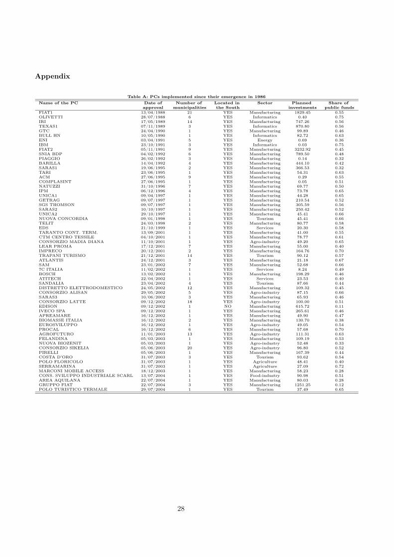
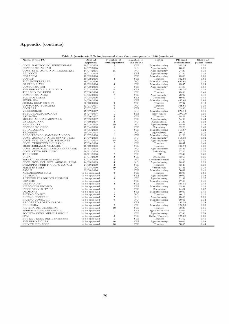
The Planning Contracts have the purpose to re-equilibrate development disparities by pro-moting large domestic and foreign industrial investments in the disadvantaged areas of theItalian territory. Table A in the Appendix lists the 121 PCs that have been implemented sincethe birth of the policy in 1986. Among the others, prominent PCs were those signed by Fiat(automobile), Barilla (food) and Texas Instruments (electronics).6

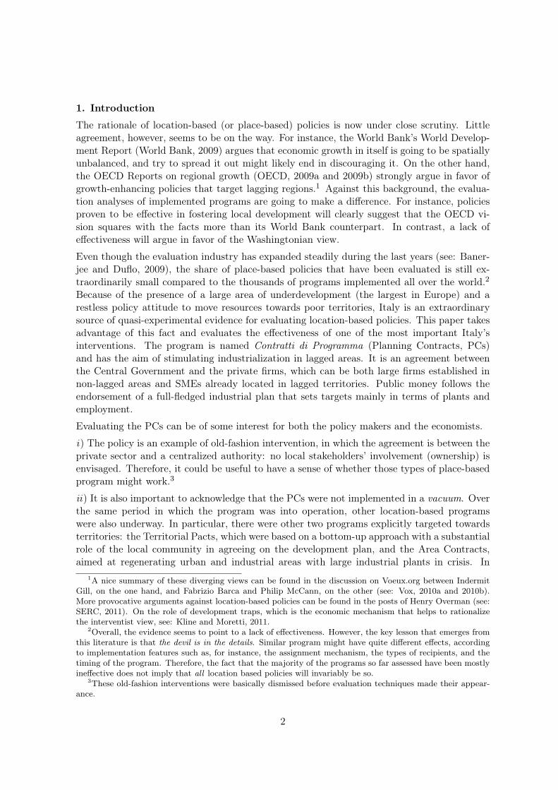
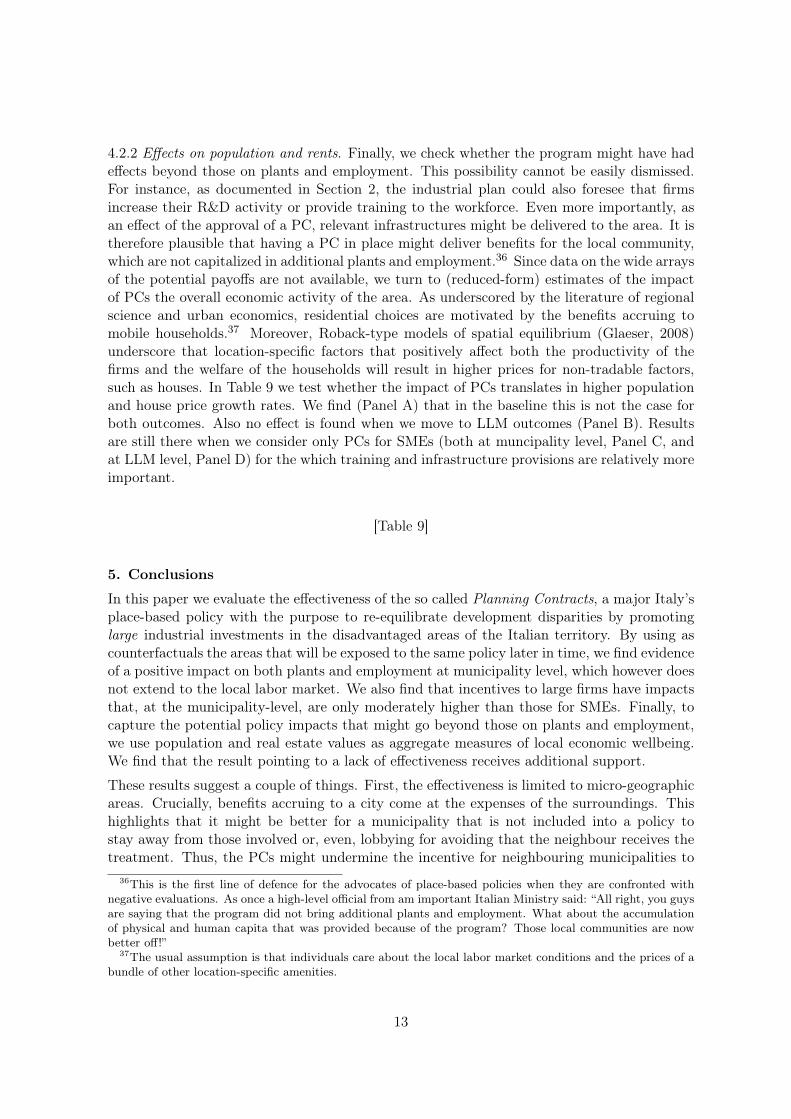
The date of approval has been quite dispersed over time (see also, Figure 1). The first twoPCs were endorsed in 1988. For more than a decade, there have been no more than few PCsapproved each year. Conversely, a surge in endorsements, also due to the availability of largerallocations following an EU decision 7, occurred at the beginning of the 2000s and in the lastyears of the decade.

[Figure 1]

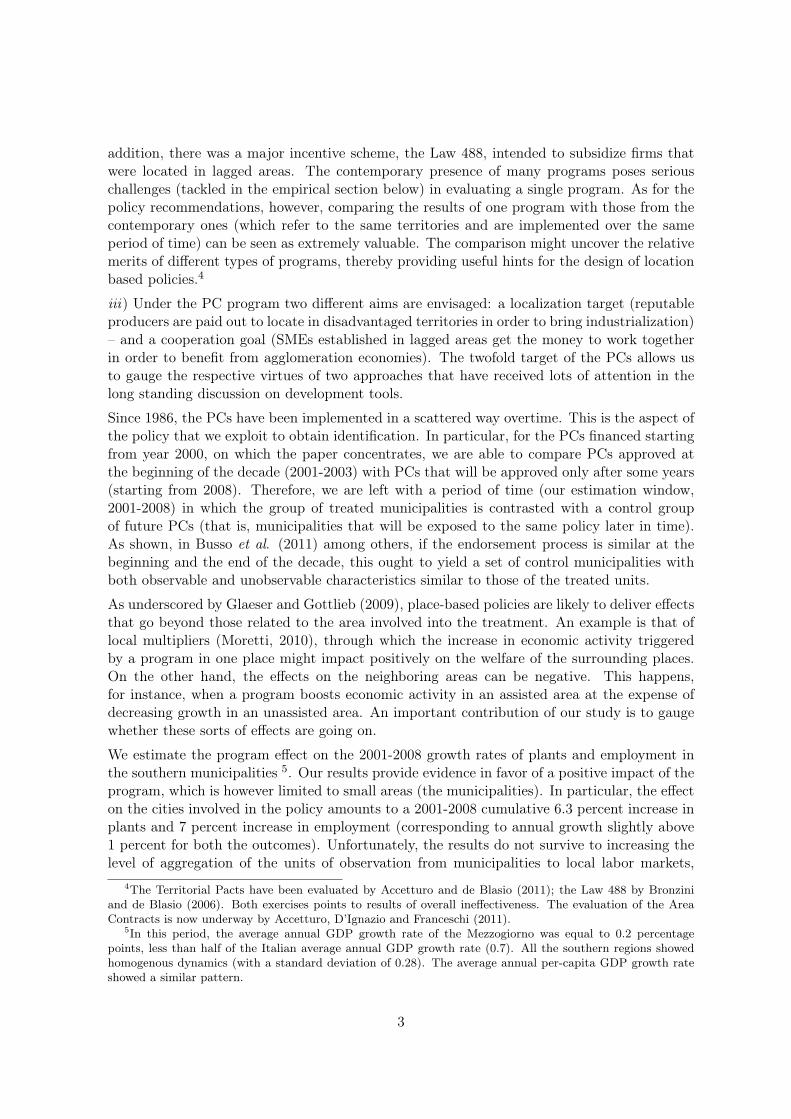
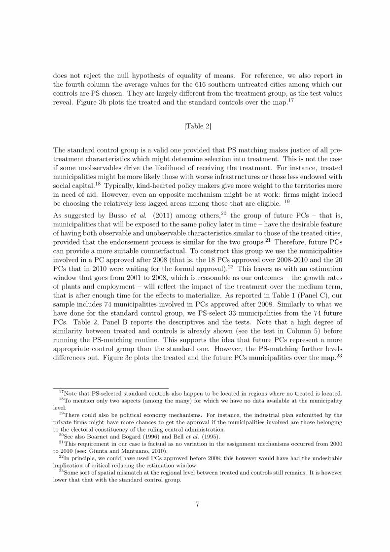
The PC initiative represents one of the major Italy’s place-based programs, in terms bothof geographic coverage and amounts involved. At the end of 2010, 413 municipalities wereexposed to the program. Total investments planned under the policy amounted to 21 billionsof Euro (40% of which are financed by public funds). As backwardness in Italy is concentratedin the South, this area is overwhelmingly considered under the policy. 103 out of the 121 PCsinclude at least one southern municipality while 67% of the overall involved municipalities arelocated in the Mezzogiorno; the share of public funds channeled towards this area is as highas 94%. Figure 2 maps, over the southern territory, the municipalities that receive the PCfinancing. All southern regions have been considered under the policy (Puglia, Sicilia and, toa lesser extent, Sardinia, have relatively been more exposed).

6The table also includes a number of PCs (20 of them) that (at the time we write the paper) were alreadyendorsed even though the formal approval had still to come (these PCs will be used, together with thoseendorsed since 2008, to construct the control groups of the future PCs; see: Section 3). The table does notinclude the 12 PCs for which the public disbursement was stopped as firms were not carrying out the investmentthat have pledged. These PCs are those that officially turned out in failures. They are not considered in theempirical exercise below. Excluding them from the exercise introduces a source of upward bias for the results.This however is not an issue, given the overall estimated ineffectiveness.

7A note of the EU Commission (n. SG (2000) D/105754) extended to PC some financing sources previouslylimited to other programs.

4

[Figure 2]

The program works on a bilateral “public-private” basis: it is an agreement between the CentralGovernment and the private firms. Once the Government announces the availability of theallocations, the firms interested in the program apply by presenting a full-fledged industrialplan, which singles out the targets mainly8 in terms of plants and employment9 and takes noteof the infrastructures needed.10 Then, a negotiation process between the two sides takes place.According to the official PC guidelines (see: Law 64/1986; CIPE deliberation 10/1994), thenegotiation process “follows the logic of the bilateral bargaining between public and privateagents to match the reciprocal goals”, and the contract is signed once the agreement is reached.On the features of the negotiate, little is known. The negotiation is conduced by an high-level policy committee (the Interdepartmental Committee for Economic Planning, CIPE ),which relies on the advices of a technical commission. During the negotiate, public authoritiesmight ask for variations to the initial plan submitted by the private firms. These requestsmight either be accommodated by the proponents or lead to refusal. Disbursement follows theendorsement according to an installment schedule, which is agreed at the time the contractis signed (and that can be stopped if the monitoring activity reveals that the firms are notcarrying out the investments that have pledged). In principle, PCs can be implemented inboth tradables and non tradables sectors. As a matter of fact, the bulk of initiatives refers tothe sectors of tourism, manufacturing and agro-industry.11 In 1990, the initiative, originallythought to stimulate large firms (or corporate groups) to locate in lagged areas, was madeavailable also to SMEs already located in depressed areas.

3. Data and empirical strategy

Information on PCs has been collected through the archive of deliberations of the Interdepart-mental Committee for Economic Planning. The effectiveness of the policy is mainly evaluatedin terms of plants and employment growth rates, for the sectors of industry and non financialservices. Data sources for both outcomes are from the Census, which is available for 2001, andthe ASIA-UL archive, which provides annually Census-type information from 2004 onwards.As the latter source only records municipalities with more than 5,000 inhabitants, our samplehas been accordingly restricted. We also make use of data on population and rents. Theyare taken, respectively, form the Italian Institute of Statistics (Istat) and the Observatory onReal Estate Market of the Territorial Agency.

The paper focuses on the PCs approved after year 2000. This allows us to get a sizable datasetby exploiting the fact that at the beginning of the decade (see: Figure 1) there was a boom

8Additional targets refer to research activity developed by the firms and training and re-qualification ofnew and old employees.

9Proponent firms must also present a detailed financial plan, which shows internal and external fundingsources.

10The industrial plan might require investment in local (material or immaterial) infrastructures, which willbe totally funded with public resources.

11Even though one of the aims of the PCs was to stimulate foreign direct investments, only 6 PCs weresigned with non Italian companies.

5

in approvals. Our treatment group is made up of PCs endorsed during the period 2001-2003.This permits us to consider the 2001 Census information as a reasonable pre-treatment date.12

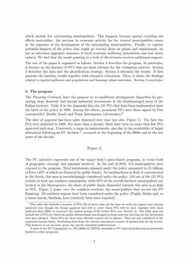
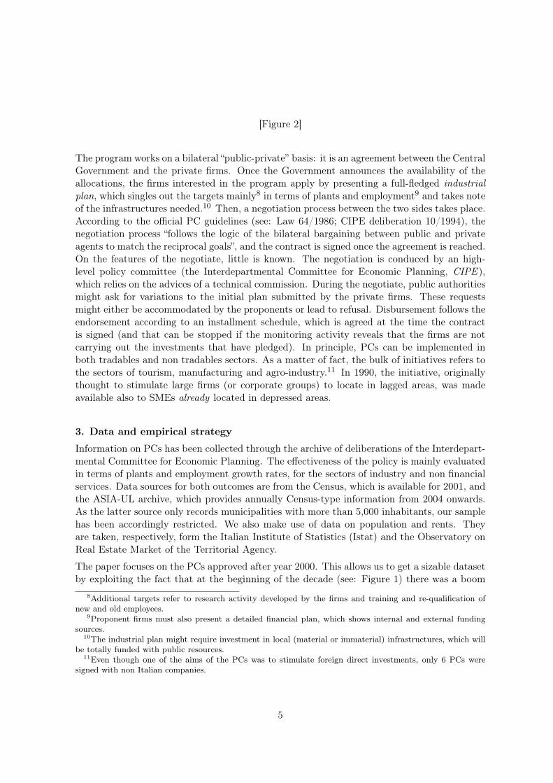
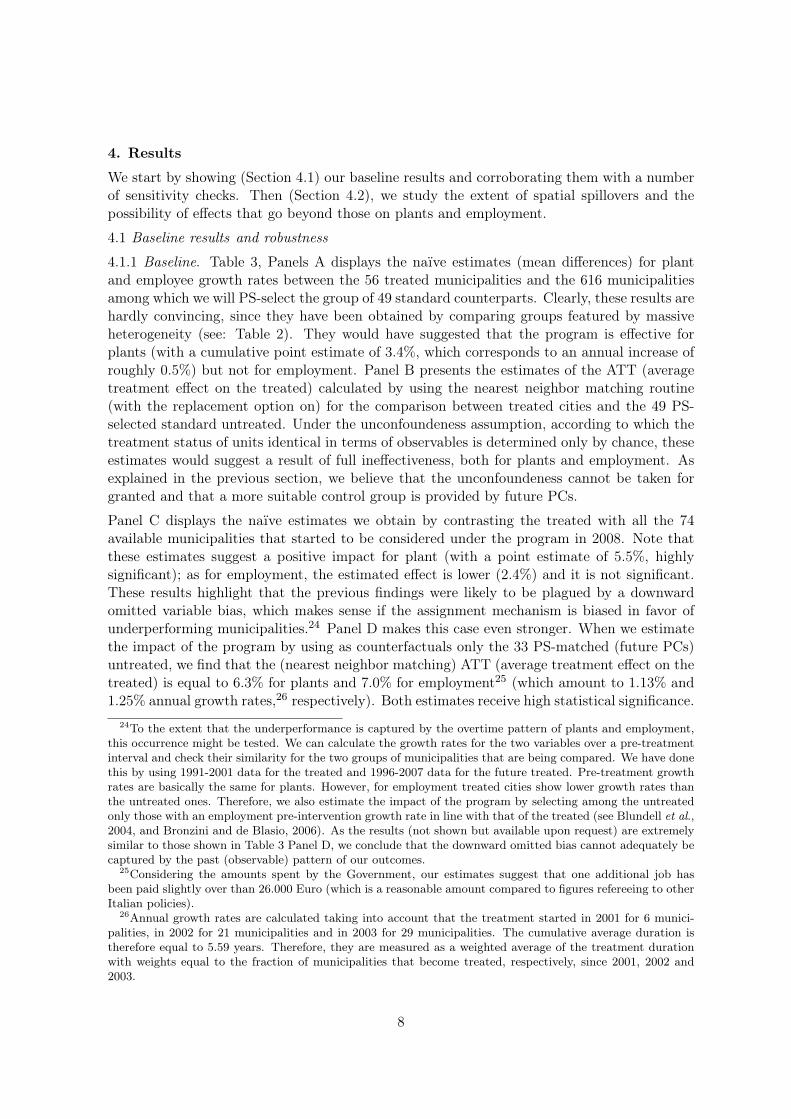
The unit of observation is the municipality.13 This represents the most detailed level of strati-fication available with the data at hand. We start with a sample of 106 municipalities involvedin 31 PCs approved in the period 2001-2003. Excluding the centre and north counterpartshas the advantage of providing a more homogenous sample, as the Mezzogiorno differs fromthe rest of the country for a multiplicity of factors, such as access to markets, infrastructures,geography, cultural habits, etc. Therefore, by focusing only on southern territories we min-imize the risk of mistakenly reflecting confounding factors, while the price we pay in termsof information loss is quite negligible (only 2 PCs14, including 4 municipalities are from theCentre North). As the program was implemented continuously from 1988 to 2010, we dropfrom the treatment group both the municipalities that are treated under PCs approved before2000 and those receiving additional treatment under PCs approved from 2004 onwards. Thisleaves us with 80 southern municipalities involved in 19 PCs approved in the period 2001-2003.As the data source for the outcomes of interest is the ASIA-UL archive, we can only focuson municipalities with more than 5,000 inhabitants. This leaves us with 56 treated cities.Table 1, Panel A summarizes the sample construction. Figure 3a plots the treatment groupover a map of the South of Italy. Treated municipalities are located in Campania, Basilicata,Calabria, Sardinia and Sicilia.

[Table 1]

[Figure 3]

Treated municipalities are contrasted with a group of control municipalities, i.e. a group ofmunicipalities that ought to mimic the behavior of the treated ones in absence of the program.The paper makes use of two control groups.

The first one is a standard one (Table 1, Panel B). It is made up of 49 municipalities selectedthrough a propensity score (PS) matching among the 616 southern municipalities that neverreceived the PC treatment. The PS-matching uses 2001 Census data at the city level for thefollowing variables: the (log of) employees, the (log of) number of plants, the (log of) surface,the activity rate, the unemployment rate, the labor productivity,15 the share of highly educatedpeople. Moreover, it uses a measure of local public spending inefficiency.16 Table 2, Panel Adescribes this sample. Pre-treatment values for the matching variables of the treated groupare described in first column. The corresponding values for the 49 control municipalities areprovided in the second column. For each variable, the p-value of the balancing property test

12Note also that the information available for our exercise is basically that provided in the Census, which isavailable only in 1981, 1991, 1996, and 2001. Therefore, only 26 out of 121 PCs approved between 1988 and2000 would have been adequately endowed with reasonable pre-treatment information.

13However, we will also provide estimates at the higher level of aggregation, which is the local labor marketthat includes the municipality (see: Section 4.2).

14One of which involves both North and South municipalities.15The productivity of labor is measured at the local labour market level.16This was generously provided by Guglielmo Barone. Details on this measure can be found in Barone and

Mocetti, 2011.

6

does not reject the null hypothesis of equality of means. For reference, we also report inthe fourth column the average values for the 616 southern untreated cities among which ourcontrols are PS chosen. They are largely different from the treatment group, as the test valuesreveal. Figure 3b plots the treated and the standard controls over the map.17

[Table 2]

The standard control group is a valid one provided that PS matching makes justice of all pre-treatment characteristics which might determine selection into treatment. This is not the caseif some unobservables drive the likelihood of receiving the treatment. For instance, treatedmunicipalities might be more likely those with worse infrastructures or those less endowed withsocial capital.18 Typically, kind-hearted policy makers give more weight to the territories morein need of aid. However, even an opposite mechanism might be at work: firms might indeedbe choosing the relatively less lagged areas among those that are eligible. 19

As suggested by Busso et al. (2011) among others,20 the group of future PCs – that is,municipalities that will be exposed to the same policy later in time – have the desirable featureof having both observable and unobservable characteristics similar to those of the treated cities,provided that the endorsement process is similar for the two groups.21 Therefore, future PCscan provide a more suitable counterfactual. To construct this group we use the municipalitiesinvolved in a PC approved after 2008 (that is, the 18 PCs approved over 2008-2010 and the 20PCs that in 2010 were waiting for the formal approval).22 This leaves us with an estimationwindow that goes from 2001 to 2008, which is reasonable as our outcomes – the growth ratesof plants and employment – will reflect the impact of the treatment over the medium term,that is after enough time for the effects to materialize. As reported in Table 1 (Panel C), oursample includes 74 municipalities involved in PCs approved after 2008. Similarly to what wehave done for the standard control group, we PS-select 33 municipalities from the 74 futurePCs. Table 2, Panel B reports the descriptives and the tests. Note that a high degree ofsimilarity between treated and controls is already shown (see the test in Column 5) beforerunning the PS-matching routine. This supports the idea that future PCs represent a moreappropriate control group than the standard one. However, the PS-matching further levelsdifferences out. Figure 3c plots the treated and the future PCs municipalities over the map.23

17Note that PS-selected standard controls also happen to be located in regions where no treated is located.18To mention only two aspects (among the many) for which we have no data available at the municipality

level.19There could also be political economy mechanisms. For instance, the industrial plan submitted by the

private firms might have more chances to get the approval if the municipalities involved are those belongingto the electoral constituency of the ruling central administration.

20See also Boarnet and Bogard (1996) and Bell et al. (1995).21This requirement in our case is factual as no variation in the assignment mechanisms occurred from 2000

to 2010 (see: Giunta and Mantuano, 2010).22In principle, we could have used PCs approved before 2008; this however would have had the undesirable

implication of critical reducing the estimation window.23Some sort of spatial mismatch at the regional level between treated and controls still remains. It is however

lower that that with the standard control group.

7

4. Results

We start by showing (Section 4.1) our baseline results and corroborating them with a numberof sensitivity checks. Then (Section 4.2), we study the extent of spatial spillovers and thepossibility of effects that go beyond those on plants and employment.

4.1 Baseline results and robustness

4.1.1 Baseline. Table 3, Panels A displays the naïve estimates (mean differences) for plantand employee growth rates between the 56 treated municipalities and the 616 municipalitiesamong which we will PS-select the group of 49 standard counterparts. Clearly, these results arehardly convincing, since they have been obtained by comparing groups featured by massiveheterogeneity (see: Table 2). They would have suggested that the program is effective forplants (with a cumulative point estimate of 3.4%, which corresponds to an annual increase ofroughly 0.5%) but not for employment. Panel B presents the estimates of the ATT (averagetreatment effect on the treated) calculated by using the nearest neighbor matching routine(with the replacement option on) for the comparison between treated cities and the 49 PS-selected standard untreated. Under the unconfoundeness assumption, according to which thetreatment status of units identical in terms of observables is determined only by chance, theseestimates would suggest a result of full ineffectiveness, both for plants and employment. Asexplained in the previous section, we believe that the unconfoundeness cannot be taken forgranted and that a more suitable control group is provided by future PCs.

Panel C displays the naïve estimates we obtain by contrasting the treated with all the 74available municipalities that started to be considered under the program in 2008. Note thatthese estimates suggest a positive impact for plant (with a point estimate of 5.5%, highlysignificant); as for employment, the estimated effect is lower (2.4%) and it is not significant.These results highlight that the previous findings were likely to be plagued by a downwardomitted variable bias, which makes sense if the assignment mechanism is biased in favor ofunderperforming municipalities.24 Panel D makes this case even stronger. When we estimatethe impact of the program by using as counterfactuals only the 33 PS-matched (future PCs)untreated, we find that the (nearest neighbor matching) ATT (average treatment effect on thetreated) is equal to 6.3% for plants and 7.0% for employment25 (which amount to 1.13% and1.25% annual growth rates,26 respectively). Both estimates receive high statistical significance.

24To the extent that the underperformance is captured by the overtime pattern of plants and employment,this occurrence might be tested. We can calculate the growth rates for the two variables over a pre-treatmentinterval and check their similarity for the two groups of municipalities that are being compared. We have donethis by using 1991-2001 data for the treated and 1996-2007 data for the future treated. Pre-treatment growthrates are basically the same for plants. However, for employment treated cities show lower growth rates thanthe untreated ones. Therefore, we also estimate the impact of the program by selecting among the untreatedonly those with an employment pre-intervention growth rate in line with that of the treated (see Blundell et al.,2004, and Bronzini and de Blasio, 2006). As the results (not shown but available upon request) are extremelysimilar to those shown in Table 3 Panel D, we conclude that the downward omitted bias cannot adequately becaptured by the past (observable) pattern of our outcomes.

25Considering the amounts spent by the Government, our estimates suggest that one additional job hasbeen paid slightly over than 26.000 Euro (which is a reasonable amount compared to figures refereeing to otherItalian policies).

26Annual growth rates are calculated taking into account that the treatment started in 2001 for 6 munici-palities, in 2002 for 21 municipalities and in 2003 for 29 municipalities. The cumulative average duration istherefore equal to 5.59 years. Therefore, they are measured as a weighted average of the treatment durationwith weights equal to the fraction of municipalities that become treated, respectively, since 2001, 2002 and2003.

8

We label this last set of results as our baseline.27

[Table 3]

4.1.2 Robustness to alternative routines. Table 4 provides a first robustness check. It showsthat our estimates are rather insensitive to using different routines to estimate the ATT (forall routines, results have been obtained under the common support restriction; see: Dehejiaand Wahba, 1999 and 2002). The nearest neighbor matching method matches each treatedwith the control unit that has the closest propensity score (i.e. the nearest neighbor) and,allowing for replacement, a control unit can be the best match for more than one treatedunit (as it happens in our case). The advantage of this method is that all treated units finda match but poor matches can occur if units with fairly different propensity score end upto be matched. Given this limitation, we follow the rule-of-thumb of double-checking thefindings with alternative routines. As highlighted by Ichino and Nannicini (2002), none ofthe available alternatives is a priori superior to the nearest neighbor matching; however, theirjoint adoption is useful to asses the robustness of the estimates. Panel A presents the resultswe obtain by using the stratification method. This method computes the ATT as a weightedaverage of the ATT computed in blocks such that within each block treated and controls haveon average the same propensity score, with weights given by the distribution of treated unitsacross blocks. This approach discards observations in blocks where either treated or controlsare absent. Panel B provides results obtained by using the radius matching method. The lattermatches treated units with controls whose propensity score belongs to a neighborhood (i.e.the radius) with a dimension that is arbitrarily chosen by the researcher. A small radius mightgenerate higher quality matches at the cost of unmatched treated units. A bigger radius mightincrease the number of matches at the cost of lower quality matches. We use a radius equalto 0.1, the minimum necessary in order not to loose unmatched treated observations. PanelC presents the results we obtain by using the kernel matching method. This routine matchesall treated units with a weighted average of all controls, with weights inversely proportionalto the distance between the propensity scores of treated and controls. As shown in the table,our evidence is robust to the choice of a particular routine, with the only exception of theestimation of the ATT for employment with the radius method.

[Table 4]

4.1.3 Robustness for concurrent programs. Next, we control for the confounding effects thatmight derive from the fact that, over our estimation period, other location-based programswere also underway. As explained in Section 1, the major concurrent programs were theTerritorial Pacts (TPs), the Area Contracts (ACs), and the Law 488 (L488). The presenceof concurrent initiatives might bias our results and the sign of the distortion is not known a

27To investigate the role of regional mismatch between treated and controls for the results reported, we havereplicated the specifications of Table 3 either by including a full set of regional fixed effects or imposing thata control must be located in the same region of its treated match (in this last experiment, the number ofuntreated PS-selected municipalities in both Panel B and Panel D are reduced). Results from these checks arehowever very similar to those shown in Table 3 (they are not reported but are available upon request).

9

priori : it will be an upward bias if treated receive also extra aid on the top of that providedby PCs; it will be a downward bias if controls are considered by the other location-basedinitiatives. Note that the overlap of programs in our sample is substantial: among the 56treated, 29 are involved in TPs, 5 in ACs, and 53 receive L488 funds (28 of which are involvedalso in the other two programs); among the 33 untreated, 18 are involved in PTs, 4 in ACs, and31 receive L488 funds (17 of which are involved also in the other two programs). Therefore,the overwhelming majority of our sample of municipalities is involved in concurrent programs.However, the extent of involvement is quite balanced between treated (96%) and controls(96%). The results shown in Table 5 are derived by computing the ATT via a weightedregression method (with the weights equal to those used to provide results in Table 3, PanelD) where, beyond the treatment indicator, we include a dummy that takes the value of oneif the city is included into a Territorial Pact, a dummy that takes the value of one if themunicipality belongs to an Area Contract and a dummy that takes the value of one if the cityreceived a non-zero share of Law 488 funds.28As matter of fact, controlling for the existenceof concomitant programs (Panel A), we find that the estimated effect of PCs is moderatelylower for both plants and employment, while remaining highly significant. Panel B presentsthe same exercise by using as measure for the L488 financing the share of funding received bythe municipality (instead of the dummy). These results are moderately higher than those ofthe baseline. All in all, it seems safe to conclude that the bias caused by concurrent policiescan be deemed as negligible for our results.

[Table 5]

4.1.4 Robustness for funding heterogeneity. An important check refers to the role of fundingfor the effectiveness. The distribution of public money across municipalities is not uniform: 3municipalities (Battipaglia, Bernalda, and Nocera Inferiore) receive an overwhelming share offunds. While the sample average amounts to 6.12 millions of Euro, dropping the 3 highest-subsidized municipalities (which correspond to the 95th percentile of the distribution of thefund shares) reduces the average injection of funds to 3.83 millions.29 Therefore, we areconcerned that these cities might be driving our results. Table 6, Panel A shows that thisis not the case: by dropping the municipalities corresponding to the 95th percentile of thefund shares distribution, the results nicely mirror those of the baseline. We also find thateffectiveness is lower for the municipalities that receive a relatively minor share of funds. PanelB estimates the impact of the program for a sample that excludes the 12 lowest-subsidizedcities (5th percentile of the distribution of funding). The results are consistently higher thanthose of the baseline. Finally, Panel C presents the results for a sample that drops boththe 5th and the 95th percentiles. The general impression is that effectiveness is higher forintermediates intensities of financing.

[Table 6]

28A more drastic robustness check would have been dropping municipalities treated under other programs(see: Accetturo and de Blasio, 2011). Given the low number of observations and the high degree of overlaps,this strategy is however not available with our data.

29A similar ranking is obtained by using the average per-capita subsidy.

10

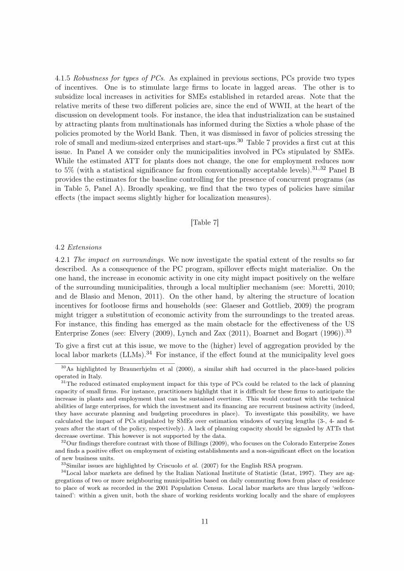
4.1.5 Robustness for types of PCs. As explained in previous sections, PCs provide two typesof incentives. One is to stimulate large firms to locate in lagged areas. The other is tosubsidize local increases in activities for SMEs established in retarded areas. Note that therelative merits of these two different policies are, since the end of WWII, at the heart of thediscussion on development tools. For instance, the idea that industrialization can be sustainedby attracting plants from multinationals has informed during the Sixties a whole phase of thepolicies promoted by the World Bank. Then, it was dismissed in favor of policies stressing therole of small and medium-sized enterprises and start-ups.30 Table 7 provides a first cut at thisissue. In Panel A we consider only the municipalities involved in PCs stipulated by SMEs.While the estimated ATT for plants does not change, the one for employment reduces nowto 5% (with a statistical significance far from conventionally acceptable levels).31,32 Panel Bprovides the estimates for the baseline controlling for the presence of concurrent programs (asin Table 5, Panel A). Broadly speaking, we find that the two types of policies have similareffects (the impact seems slightly higher for localization measures).

[Table 7]

4.2 Extensions

4.2.1 The impact on surroundings. We now investigate the spatial extent of the results so fardescribed. As a consequence of the PC program, spillover effects might materialize. On theone hand, the increase in economic activity in one city might impact positively on the welfareof the surrounding municipalities, through a local multiplier mechanism (see: Moretti, 2010;and de Blasio and Menon, 2011). On the other hand, by altering the structure of locationincentives for footloose firms and households (see: Glaeser and Gottlieb, 2009) the programmight trigger a substitution of economic activity from the surroundings to the treated areas.For instance, this finding has emerged as the main obstacle for the effectiveness of the USEnterprise Zones (see: Elvery (2009), Lynch and Zax (2011), Boarnet and Bogart (1996)).33

To give a first cut at this issue, we move to the (higher) level of aggregation provided by thelocal labor markets (LLMs).34 For instance, if the effect found at the municipality level goes

30As highlighted by Braunerhjelm et al (2000), a similar shift had occurred in the place-based policiesoperated in Italy.

31The reduced estimated employment impact for this type of PCs could be related to the lack of planningcapacity of small firms. For instance, practitioners highlight that it is difficult for these firms to anticipate theincrease in plants and employment that can be sustained overtime. This would contrast with the technicalabilities of large enterprises, for which the investment and its financing are recurrent business activity (indeed,they have accurate planning and budgeting procedures in place). To investigate this possibility, we havecalculated the impact of PCs stipulated by SMEs over estimation windows of varying lengths (3-, 4- and 6-years after the start of the policy, respectively). A lack of planning capacity should be signaled by ATTs thatdecrease overtime. This however is not supported by the data.

32Our findings therefore contrast with those of Billings (2009), who focuses on the Colorado Enterprise Zonesand finds a positive effect on employment of existing establishments and a non-significant effect on the locationof new business units.

33Similar issues are highlighted by Criscuolo et al. (2007) for the English RSA program.34Local labor markets are defined by the Italian National Institute of Statistic (Istat, 1997). They are ag-

gregations of two or more neighbouring municipalities based on daily commuting flows from place of residenceto place of work as recorded in the 2001 Population Census. Local labor markets are thus largely ‘selfcon-tained’: within a given unit, both the share of working residents working locally and the share of employees

11

hand in hand with a similar impact at the LLM level - which also includes surrounding mu-nicipalities - then positive spillovers are called for. Table 8, Panel A provides the estimates forthe baseline where the outcomes at the municipality-level have been replaced by the outcomesat the LLM-level for each of the 56 traded and 33 controls. These results point to an impactthat is quite reduced for plants and basically zero for employment.

The fact that the impact is lost by moving from city to LLM can in principle be due to the factthat the other municipalities in the control LLM receive aid from the concurrent location-basedprograms while this does not happen for the municipalities in the treated LLM. However, thisdoes not happen to be the case. Panel B provides the estimates obtained by controlling forthe presence of alterative funding at the level of LLM. In particular, we focus only on LLMsin which no other municipality (but the treated or the untreated cities, for which we have theappropriate controls – those of the specification of Table 5, Panel A – in place) is involved inconcurrent programs. Results suggest that the lack of impact at the LLM level is unlikely tobe driven by the existence of concurrent programs.

Note that the results in the first two panels of Table 8 are derived by replacing the outcomes atthe municipality level with the same outcomes at the LLM level for our sample of PS-selectedfuture PCs municipalities. These experiments highlight what happens at the higher level ofaggregation for the municipalities for which the analysis has been so far conducted. However,the appropriateness of the two groups of treated and controls can be questioned as it is derivedby comparing units at the municipality level (and not at the LLM one). To lesser this concern,Table 8, Panel C provides the results we obtain by replicating the entire exercise at the LLMlevel. Therefore, we start from the treated LLMs (over the 2001-2003 period) and comparethem with PS-selected LLMs among of future PCs. Again, for this sample (which includes30 treated and 14 untreated local labor markets) we find that the program at this level ofaggregation does not show to be effective in increasing both plants and unemployment.

In principle, the fact that the effect on municipalities evaporates by moving to local labor mar-kets might be due to the dilution of the treatment over a wider area (attenuation). However,by comparing the outcome performances of untreated municipalities located in treated LLMswith the performances of untreated municipalities located in untreated LLMs (Table 8, PanelD), we find that the first ones do worse than the latter.35 Altogether, these results suggestthat spatial substitution, not attenuation, is behind our findings.

[Table 8]

residing locally must be at least 75%. This definition is consistent with standard definitions of cities in urbaneconomics that define them through commuting patterns. It is also consistent with the notion of ‘functionalregion’, defined as ‘a territorial unit resulting from the organization of social and economic relations in that itsboundaries do not reflect geographical particularities or historical events’ (OECD, 2002). Italian local labormarkets also roughly follow the criteria used to define Metropolitan Statistical Areas in the US, Travel to WorkAreas in the UK, or Metropolitan areas and employment areas in France. Italian local labor markets span theentire national territory. In 2001, 686 of them were defined. They had an average population of 83,084 and astandard deviation of 222,418.

35Results are obtained by replacing each treated and control municipality outcome with weighted averagesof the outcomes for the surrounding untreated municipalities (with weights proportional to their surface andpopulation).

12

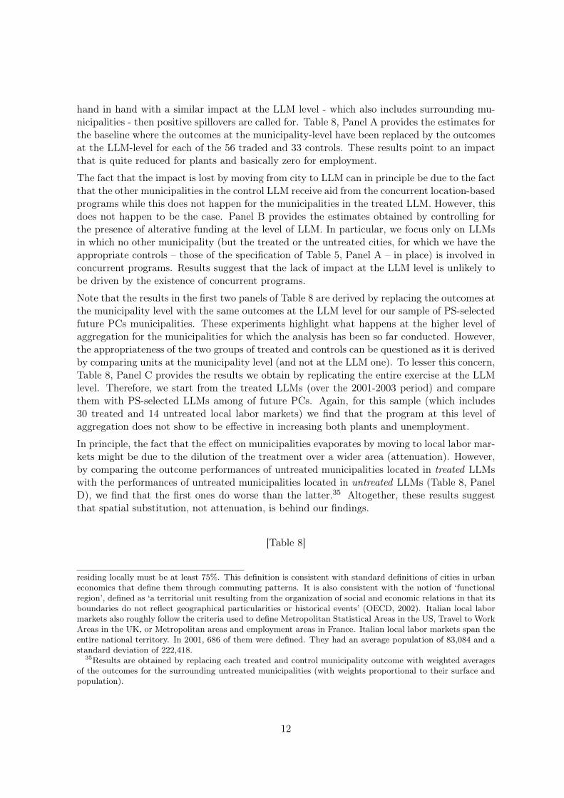
4.2.2 Effects on population and rents. Finally, we check whether the program might have hadeffects beyond those on plants and employment. This possibility cannot be easily dismissed.For instance, as documented in Section 2, the industrial plan could also foresee that firmsincrease their R&D activity or provide training to the workforce. Even more importantly, asan effect of the approval of a PC, relevant infrastructures might be delivered to the area. It istherefore plausible that having a PC in place might deliver benefits for the local community,which are not capitalized in additional plants and employment.36 Since data on the wide arraysof the potential payoffs are not available, we turn to (reduced-form) estimates of the impactof PCs the overall economic activity of the area. As underscored by the literature of regionalscience and urban economics, residential choices are motivated by the benefits accruing tomobile households.37 Moreover, Roback-type models of spatial equilibrium (Glaeser, 2008)underscore that location-specific factors that positively affect both the productivity of thefirms and the welfare of the households will result in higher prices for non-tradable factors,such as houses. In Table 9 we test whether the impact of PCs translates in higher populationand house price growth rates. We find (Panel A) that in the baseline this is not the case forboth outcomes. Also no effect is found when we move to LLM outcomes (Panel B). Resultsare still there when we consider only PCs for SMEs (both at muncipality level, Panel C, andat LLM level, Panel D) for the which training and infrastructure provisions are relatively moreimportant.

[Table 9]

5. Conclusions

In this paper we evaluate the effectiveness of the so called Planning Contracts, a major Italy’splace-based policy with the purpose to re-equilibrate development disparities by promotinglarge industrial investments in the disadvantaged areas of the Italian territory. By using ascounterfactuals the areas that will be exposed to the same policy later in time, we find evidenceof a positive impact on both plants and employment at municipality level, which however doesnot extend to the local labor market. We also find that incentives to large firms have impactsthat, at the municipality-level, are only moderately higher than those for SMEs. Finally, tocapture the potential policy impacts that might go beyond those on plants and employment,we use population and real estate values as aggregate measures of local economic wellbeing.We find that the result pointing to a lack of effectiveness receives additional support.

These results suggest a couple of things. First, the effectiveness is limited to micro-geographicareas. Crucially, benefits accruing to a city come at the expenses of the surroundings. Thishighlights that it might be better for a municipality that is not included into a policy tostay away from those involved or, even, lobbying for avoiding that the neighbour receives thetreatment. Thus, the PCs might undermine the incentive for neighbouring municipalities to

36This is the first line of defence for the advocates of place-based policies when they are confronted withnegative evaluations. As once a high-level official from am important Italian Ministry said: “All right, you guysare saying that the program did not bring additional plants and employment. What about the accumulationof physical and human capita that was provided because of the program? Those local communities are nowbetter off!”

37The usual assumption is that individuals care about the local labor market conditions and the prices of abundle of other location-specific amenities.

13

work together to improve their economic conditions. Second, this piece of evidence has tobe read against the background of the disappointing results of other place-based policies inItaly. This highlights that in the case of this country (very unfortunately) the devil is notin the details. On the contrary, irrespectively of the single details of the program (that isirrespectively of the bottom-up/top-down approach; the fact that money goes to large/smallfirms; the assignment mechanism; etc), a lack of effectiveness prevails.

14

References

Accetturo A. and de Blasio G. (2011), Policies for Local Development: an Evaluation of Italy’s«Patti Territoriali», Regional Science and Urban Economics, 42 (1-2):15-26.

Accetturo A., D’Ingrazio A. and Franceschi F. (2011), Make up for large industrial plantsclosures: assessing the effectiveness of an Italian policy, mimeo, Bank of Italy.

Banerjee A. V. and Duflo E. (2009), http: // ideas. repec. org/ a/ anr/ reveco/v1y2009p151-178. html , http://ideas.repec.org/s/anr/reveco.html, Annual Reviews,1(1): 151-178.

Barca F. and McCann P. (2010), The Place Based Approach: A Response to Mr. Gill, availableat: http://www.voxeu.org/index.php?q=node/5644.

Barone G. and Mocetti S. (2011), Tax Morale and Public Spending Inefficiency, InternationalTax and Public Finance, 18(6):724-749.

Bell S., Orr L., Blomquist J., and Cain G. (1995), Program Applicants as a Comparison Groupin Evaluating Training Programs: Theory and a Test. Kalamazoo, MI: W.E. Upjohn Institutefor Employment Research.

Billings S. (2009), Do Enterprise Zones Work? An Analysis at the Borders, Public FinanceReview, 37(1): 68-93.

Blundell R., Costa Dias M., Meghir C. and Van Reenen J. (2004), Evaluating the EmploymentImpact of a Mandatory Job Search Program, Journal of the European Economic Association,2(4): 569-606.

Boarnet M. and Bogart W. (1996), Enterprise Zones and Employment: Evidence from NewJersey, Journal of Urban Economics, 40, 198-215.

Braunerhjelm P., Faini R., Norman V., Ruane F. and Seabright P. (2000), Integration andthe Regiones of Europe: How the Right Policies Can Prevent Polarization, London, Centre forEconomic Policy Research.

Bronzini R. and de Blasio G. (2006), Evaluating the Impact of Investment Incentives: the Caseof Italy’s Law 488/92, Journal of Urban Economics, 60 (2): 327-349.

Busso M., Gregory J and Kline P (2011), http: // ideas. repec. org/ p/ cen/ wpaper/11-07. html , Working Paper 11-07, Center for Economic Studies, U.S. Census Bureau. (Pre-vious version: Busso M., Gregory J and Kline P (2010), http: // ideas. repec. org/ p/cen/ wpaper/ 11-07. html , http://ideas.repec.org/s/nbr/nberwo.html 16096, NationalBureau of Economic Research)

de Blasio G., and Menon C. (2011), Local effects of Manufacturing employment growth inItaly, Giornale degli Economisti, forthcoming.

Dehejia R. and Wahba S. (1999), Causal Effects in Non-Experimental Studies: Re-Evaluatingthe Evaluation of Training Programs, Journal of the American Statistical Association, 94:1053–1062.

Dehejia R. and Wahba S. (2002), Propensity Score-Matching Methods for Non-experimentalCausal Studies, The Review of Economics and Statistics, 84: 151-161.

Elvery J. (2009), Enterprise Zones and Resident Employment: An Evaluation of the EnterpriseZone Programs of California and Florida, Economic Development Quarterly, 23(1): 44-59.

15

Glaeser E. (2008), Cities, Agglomeration and Spatial Equilibrium, Oxford University Press.

Glaeser E. and Gottlieb J. (2009), The Wealth of Cities: Agglomeration Economies and SpatialEquilibrium in the United States, Journal of Economic Literature, 47(4): 983–1028.

Gill I. (2010), http: // www. voxeu. org/ index. php? q= node/ 5644 , available at: http://www.voxeu.org/index.php?q=node/5644.

Giunta A. and Mantuano M. (2010), Contratti di Programma: Evoluzione della Normativa edEfficacia Economica, Economia e Politica Industriale, 1: 151-166.

Holmes T. (1998), The Effects of State Policies on the Location of Industry: Evidence fromState Borders, Journal of Political Economy, 106(4): 667-705.

Ichino A. and Nannicini T. (2002), Estimation of Average Treatment Effects based on Propen-sity Scores, http://www.stata-journal.com (2002) 4(2): 358-377.

Kline P. and Moretti E. (2011), Local Economic Development, Agglomeration Economies andthe Big Push: 100 Years of Evidence from the Tennessee Valley Authority, mimeo.

Lynch D. and Zax J.S. (2011), http: // ideas. repec. org/ a/ sae/ pubfin/v39y2011i2p226-255. html , Public Finance Review, 39(2): 226-255.

Moretti E. (2010), Local Multipliers, American Economic Review: Papers and Proceedings,100: 1-7.

OECD (2009a), How Regions Grow: Trends and Analysis, OECD, Paris.

OECD (2009b), Regions at a Glance 2009, OECD, Paris.

Overman H. (2011), Blogspot of the LSE Spatial Econometrics Research Center,

available at: http://spatial-economics.blogspot.com/2011.

World Bank (2009), Reshaping Economic Geography : World Development Report, WorldBank, Washington, DC.

16

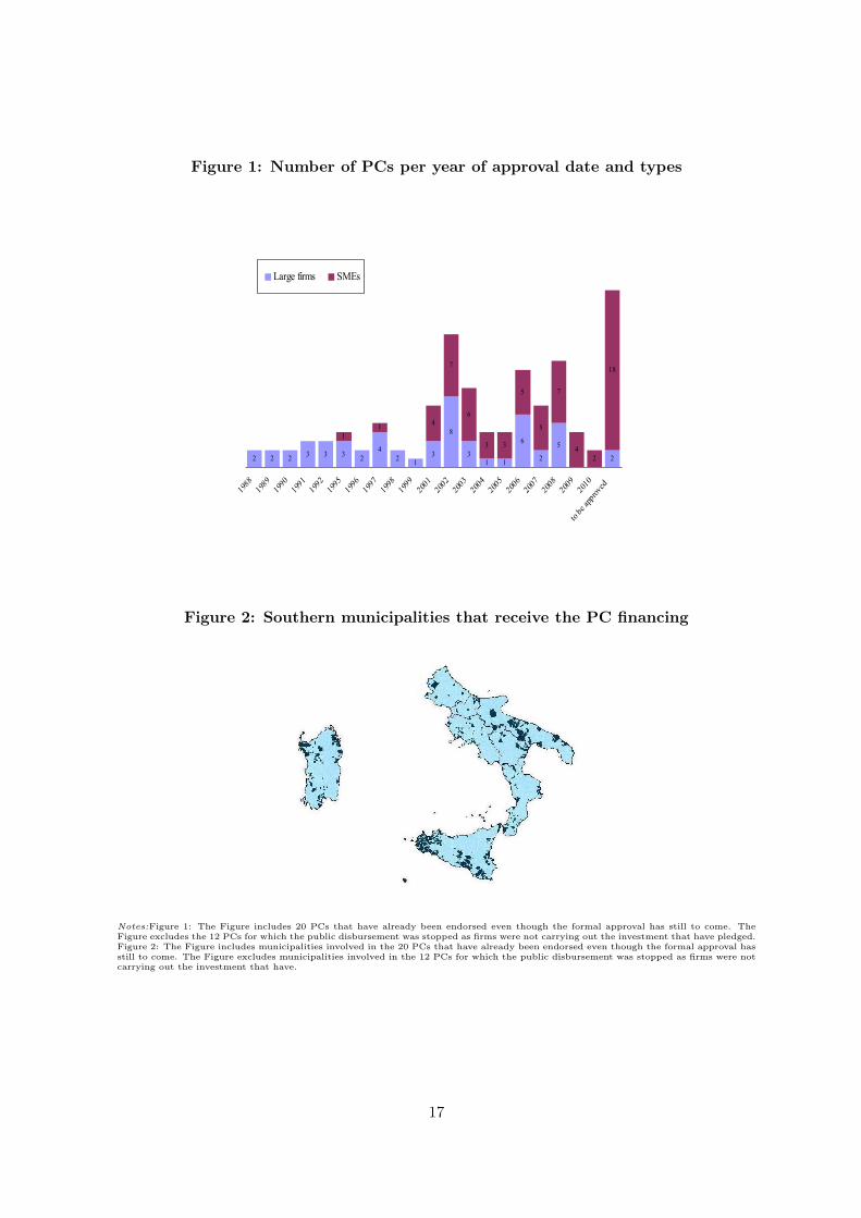
Figure 1: Number of PCs per year of approval date and types

2 2 2 3 3 3 24

2 13

8

31 1

6

2

5

2

11 4

7

6

3 3

5

5

7

42

18

1988

1989

1990

1991

1992

1995

1996

1997

1998

1999

2001

2002

2003

2004

2005

2006

2007

2008

2009

2010

to be

appro

ved

Large firms SMEs

Figure 2: Southern municipalities that receive the PC financing

Notes:Figure 1: The Figure includes 20 PCs that have already been endorsed even though the formal approval has still to come. TheFigure excludes the 12 PCs for which the public disbursement was stopped as firms were not carrying out the investment that have pledged.Figure 2: The Figure includes municipalities involved in the 20 PCs that have already been endorsed even though the formal approval hasstill to come. The Figure excludes municipalities involved in the 12 PCs for which the public disbursement was stopped as firms were notcarrying out the investment that have.

17

Figure 3: Municipalities in the sample

Figure 3a: Treated municipalities

Figure 3b: Treated and (PS-Selected Standard) Controls

Figure 3c: Treated and (PS-Selected Future PCs) Controls

Notes:Figure 3a: Treated group (56 municipalities involved in PCs in the period 2001-2003.) over the map of the South of Italy. Both themunicipalities that are treated under PCs approved before 2000 and those receiving additional treatment under PCs approved from 2004onwards have been excluded. Figures 3b: Treated municipalities (dark blue); PS-Selected Standard control municipalities (light blue).To construct the control group the PS-matching has been used. Figures 3c: Treated municipalities (dark blue); PS-Selected Future PCscontrol municipalities (light blue). To construct the control group we use the municipalities involved in the PCs approved after 2008. ThePS-matching uses 2001 Census data at the city level for the following variables: the (log of) employees, the (log of) number of plants, the(log of) surface, the activity rate, the unemployment rate, the labor productivity , the share of highly educated people, and a measure oflocal public spending inefficiency (provided by Barone and Mocetti, 2011).

18

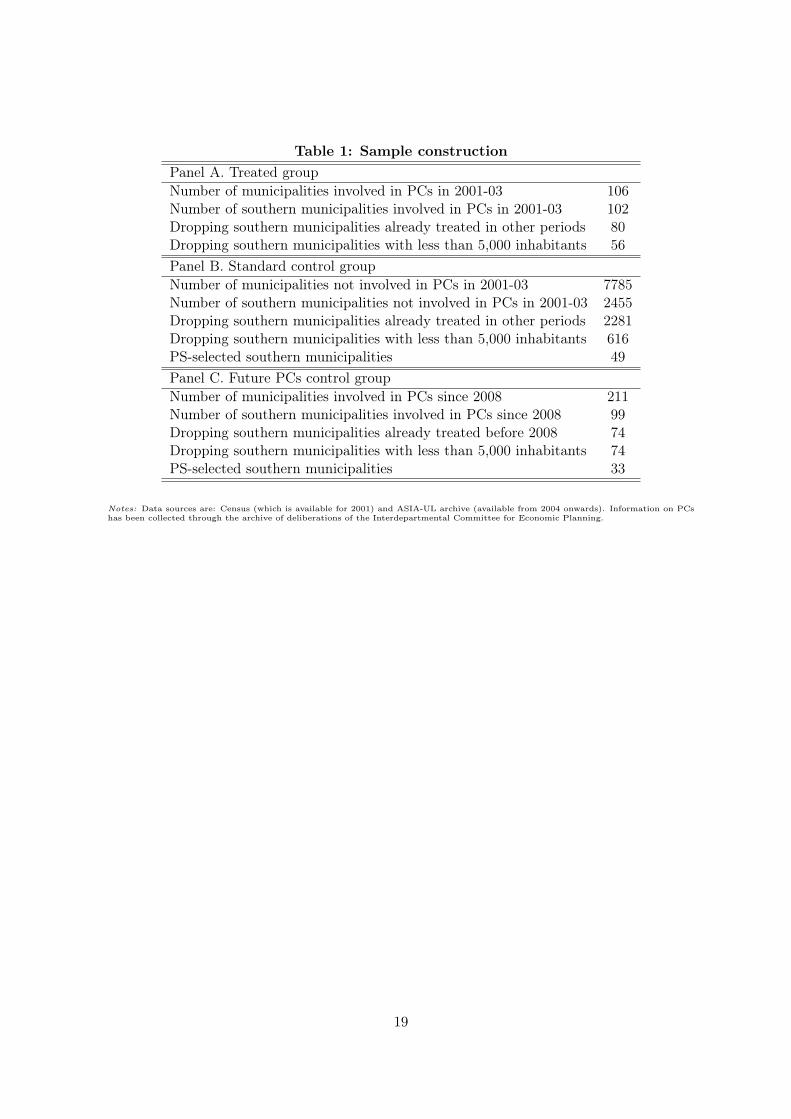
Table 1: Sample constructionPanel A. Treated groupNumber of municipalities involved in PCs in 2001-03 106Number of southern municipalities involved in PCs in 2001-03 102Dropping southern municipalities already treated in other periods 80Dropping southern municipalities with less than 5,000 inhabitants 56Panel B. Standard control groupNumber of municipalities not involved in PCs in 2001-03 7785Number of southern municipalities not involved in PCs in 2001-03 2455Dropping southern municipalities already treated in other periods 2281Dropping southern municipalities with less than 5,000 inhabitants 616PS-selected southern municipalities 49Panel C. Future PCs control groupNumber of municipalities involved in PCs since 2008 211Number of southern municipalities involved in PCs since 2008 99Dropping southern municipalities already treated before 2008 74Dropping southern municipalities with less than 5,000 inhabitants 74PS-selected southern municipalities 33

Notes: Data sources are: Census (which is available for 2001) and ASIA-UL archive (available from 2004 onwards). Information on PCshas been collected through the archive of deliberations of the Interdepartmental Committee for Economic Planning.

19

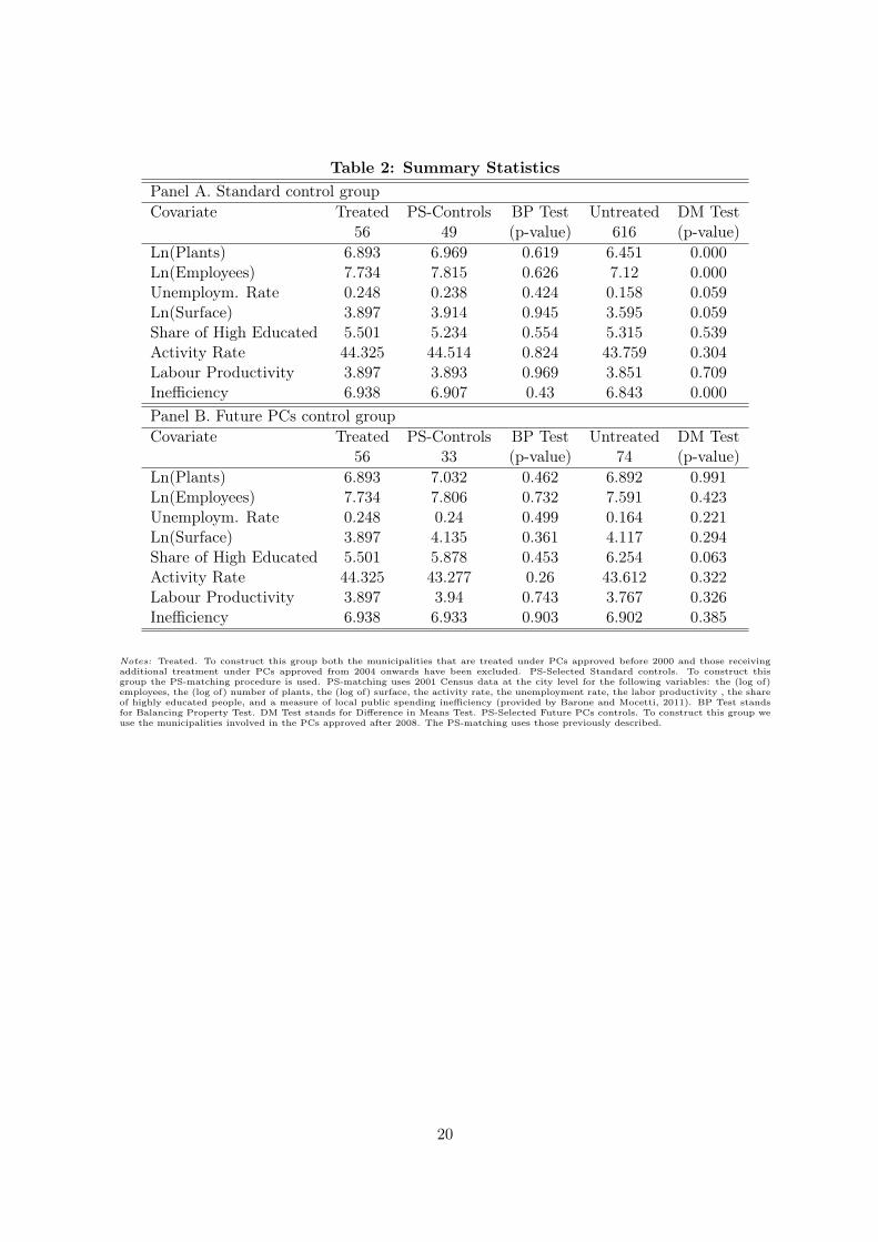
Table 2: Summary StatisticsPanel A. Standard control groupCovariate Treated PS-Controls BP Test Untreated DM Test

56 49 (p-value) 616 (p-value)Ln(Plants) 6.893 6.969 0.619 6.451 0.000Ln(Employees) 7.734 7.815 0.626 7.12 0.000Unemploym. Rate 0.248 0.238 0.424 0.158 0.059Ln(Surface) 3.897 3.914 0.945 3.595 0.059Share of High Educated 5.501 5.234 0.554 5.315 0.539Activity Rate 44.325 44.514 0.824 43.759 0.304Labour Productivity 3.897 3.893 0.969 3.851 0.709Inefficiency 6.938 6.907 0.43 6.843 0.000Panel B. Future PCs control groupCovariate Treated PS-Controls BP Test Untreated DM Test

56 33 (p-value) 74 (p-value)Ln(Plants) 6.893 7.032 0.462 6.892 0.991Ln(Employees) 7.734 7.806 0.732 7.591 0.423Unemploym. Rate 0.248 0.24 0.499 0.164 0.221Ln(Surface) 3.897 4.135 0.361 4.117 0.294Share of High Educated 5.501 5.878 0.453 6.254 0.063Activity Rate 44.325 43.277 0.26 43.612 0.322Labour Productivity 3.897 3.94 0.743 3.767 0.326Inefficiency 6.938 6.933 0.903 6.902 0.385

Notes: Treated. To construct this group both the municipalities that are treated under PCs approved before 2000 and those receivingadditional treatment under PCs approved from 2004 onwards have been excluded. PS-Selected Standard controls. To construct thisgroup the PS-matching procedure is used. PS-matching uses 2001 Census data at the city level for the following variables: the (log of)employees, the (log of) number of plants, the (log of) surface, the activity rate, the unemployment rate, the labor productivity , the shareof highly educated people, and a measure of local public spending inefficiency (provided by Barone and Mocetti, 2011). BP Test standsfor Balancing Property Test. DM Test stands for Difference in Means Test. PS-Selected Future PCs controls. To construct this group weuse the municipalities involved in the PCs approved after 2008. The PS-matching uses those previously described.

20

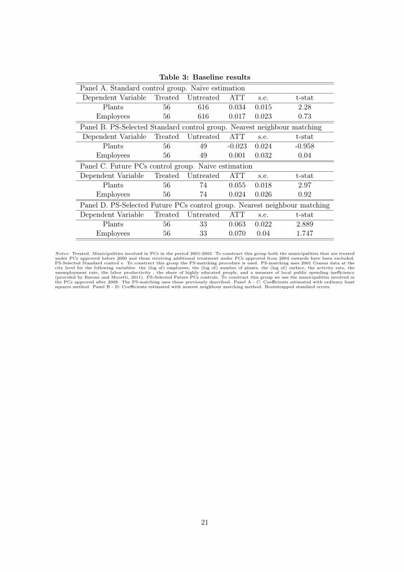
Table 3: Baseline resultsPanel A. Standard control group. Naive estimationDependent Variable Treated Untreated ATT s.e. t-stat

Plants 56 616 0.034 0.015 2.28Employees 56 616 0.017 0.023 0.73

Panel B. PS-Selected Standard control group. Nearest neighbour matchingDependent Variable Treated Untreated ATT s.e. t-stat

Plants 56 49 -0.023 0.024 -0.958Employees 56 49 0.001 0.032 0.04

Panel C. Future PCs control group. Naive estimationDependent Variable Treated Untreated ATT s.e. t-stat


Panel D. PS-Selected Future PCs control group. Nearest neighbour matchingDependent Variable Treated Untreated ATT s.e. t-stat


Notes: Treated. Municipalities involved in PCs in the period 2001-2003. To construct this group both the municipalities that are treatedunder PCs approved before 2000 and those receiving additional treatment under PCs approved from 2004 onwards have been excluded.PS-Selected Standard control s. To construct this group the PS-matching procedure is used. PS-matching uses 2001 Census data at thecity level for the following variables: the (log of) employees, the (log of) number of plants, the (log of) surface, the activity rate, theunemployment rate, the labor productivity , the share of highly educated people, and a measure of local public spending inefficiency(provided by Barone and Mocetti, 2011). PS-Selected Future PCs controls. To construct this group we use the municipalities involved inthe PCs approved after 2008. The PS-matching uses those previously described. Panel A - C: Coefficients estimated with ordinary leastsquares method. Panel B - D: Coefficients estimated with nearest neighbour matching method. Bootstrapped standard errors.

21

Table 4: Robustness for alternative matching routinesPanel A. Stratification matchingDependent Variable Treated Untreated ATT s.e. t-stat


Panel B. Radius matchingDependent Variable Treated Untreated ATT s.e. t-stat


Panel C. Kernel matchingDependent Variable Treated Untreated ATT s.e. t-stat


Notes: Treated. Municipalities involved in PCs in the period 2001-2003. To construct this group both the municipalities that are treatedunder PCs approved before 2000 and those receiving additional treatment under PCs approved from 2004 onwards have been excluded.PS-Selected Future PCs controls. To construct this group we use the municipalities involved in the PCs approved after 2008. The PS-matching uses 2001 Census data at the city level for the following variables: the (log of) employees, the (log of) number of plants, the (logof) surface, the activity rate, the unemployment rate, the labor productivity , the share of highly educated people, and a measure of localpublic spending inefficiency (provided by Barone and Mocetti, 2011). Panel B: ATT estimated with radius equal to 0.1. Bootstrappedstandard errors.

22

Table 5: Robustness for concurrent programsPanel A. Dummy for TP and AC; Dummy for Law 488Dependent Variable Treated Untreated ATT s.e. t-stat


Panel B. Dummy for TP and AC; Share of financing for Law 488Dependent Variable Treated Untreated ATT s.e. t-stat


Notes: Treated. Municipalities involved in PCs in the period 2001-2003. To construct this group both the municipalities that are treatedunder PCs approved before 2000 and those receiving additional treatment under PCs approved from 2004 onwards have been excluded.PS-Selected Future PCs controls. To construct this group we use the municipalities involved in the PCs approved after 2008. The PS-matching uses 2001 Census data at the city level for the following variables: the (log of) employees, the (log of) number of plants, the (logof) surface, the activity rate, the unemployment rate, the labor productivity , the share of highly educated people, and a measure of localpublic spending inefficiency (provided by Barone and Mocetti, 2011). ATT estimated with weighted regression method. Robust standarderrors.

23

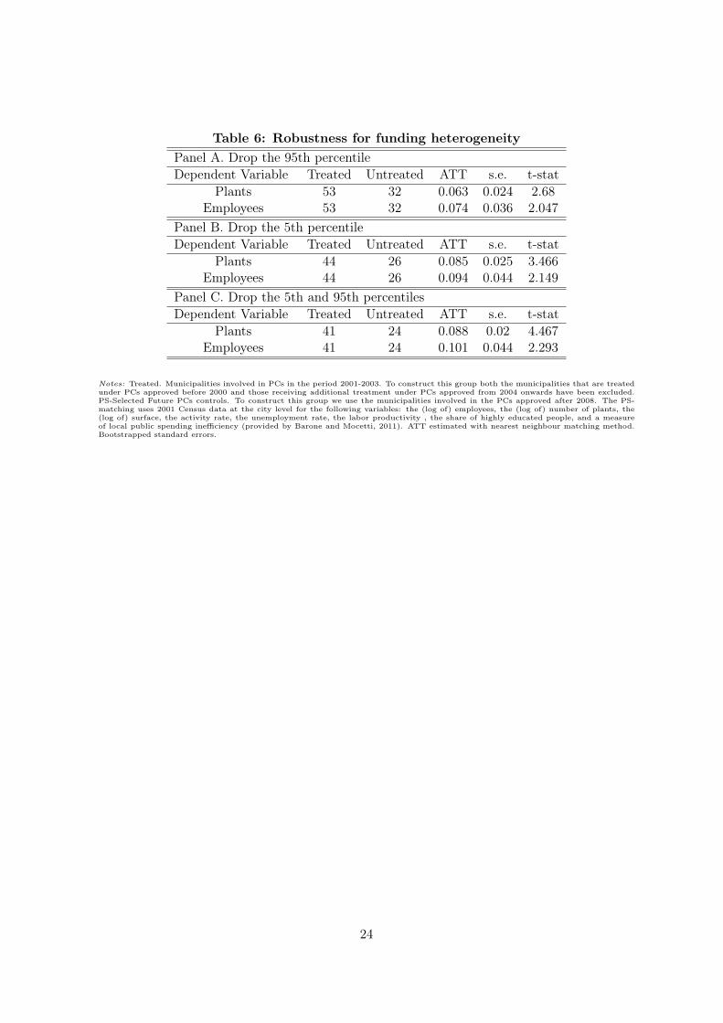
Table 6: Robustness for funding heterogeneityPanel A. Drop the 95th percentileDependent Variable Treated Untreated ATT s.e. t-stat


Panel B. Drop the 5th percentileDependent Variable Treated Untreated ATT s.e. t-stat


Panel C. Drop the 5th and 95th percentilesDependent Variable Treated Untreated ATT s.e. t-stat


Notes: Treated. Municipalities involved in PCs in the period 2001-2003. To construct this group both the municipalities that are treatedunder PCs approved before 2000 and those receiving additional treatment under PCs approved from 2004 onwards have been excluded.PS-Selected Future PCs controls. To construct this group we use the municipalities involved in the PCs approved after 2008. The PS-matching uses 2001 Census data at the city level for the following variables: the (log of) employees, the (log of) number of plants, the(log of) surface, the activity rate, the unemployment rate, the labor productivity , the share of highly educated people, and a measureof local public spending inefficiency (provided by Barone and Mocetti, 2011). ATT estimated with nearest neighbour matching method.Bootstrapped standard errors.

24

Table 7: Robustness for types of PCsPanel A. Only SMEsDependent Variable Treated Untreated ATT s.e. t-stat


Panel B. Only SMEs. Controlling for concurrent programsDependent Variable Treated Untreated ATT s.e. t-stat


Notes: Treated. Municipalities involved in PCs in the period 2001-2003. To construct this group both the municipalities that are treatedunder PCs approved before 2000 and those receiving additional treatment under PCs approved from 2004 onwards have been excluded.PS-Selected Future PCs controls. To construct this group we use the municipalities involved in the PCs approved after 2008. The PS-matching uses 2001 Census data at the city level for the following variables: the (log of) employees, the (log of) number of plants, the(log of) surface, the activity rate, the unemployment rate, the labor productivity , the share of highly educated people, and a measureof local public spending inefficiency (provided by Barone and Mocetti, 2011). ATT estimated with nearest neighbour matching method.Bootstrapped standard errors.

25

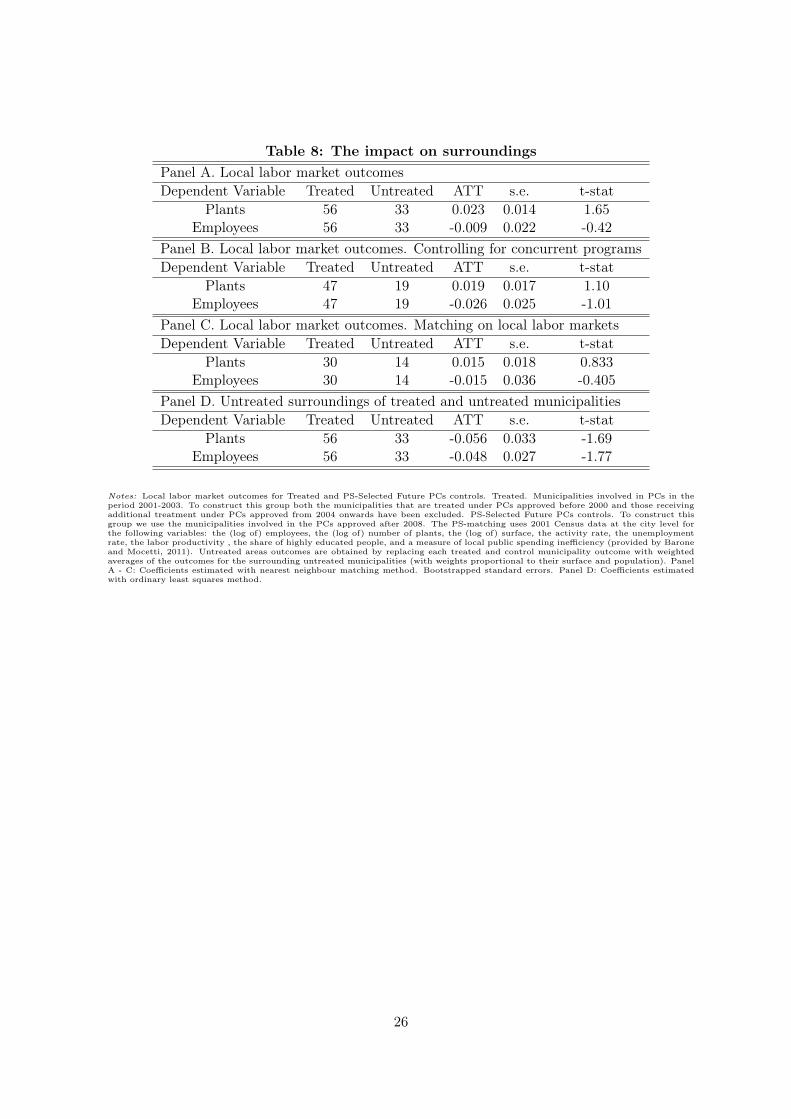
Table 8: The impact on surroundingsPanel A. Local labor market outcomesDependent Variable Treated Untreated ATT s.e. t-stat

Plants 56 33 0.023 0.014 1.65Employees 56 33 -0.009 0.022 -0.42

Panel B. Local labor market outcomes. Controlling for concurrent programsDependent Variable Treated Untreated ATT s.e. t-stat


Panel C. Local labor market outcomes. Matching on local labor marketsDependent Variable Treated Untreated ATT s.e. t-stat


Panel D. Untreated surroundings of treated and untreated municipalitiesDependent Variable Treated Untreated ATT s.e. t-stat

Plants 56 33 -0.056 0.033 -1.69Employees 56 33 -0.048 0.027 -1.77

Notes: Local labor market outcomes for Treated and PS-Selected Future PCs controls. Treated. Municipalities involved in PCs in theperiod 2001-2003. To construct this group both the municipalities that are treated under PCs approved before 2000 and those receivingadditional treatment under PCs approved from 2004 onwards have been excluded. PS-Selected Future PCs controls. To construct thisgroup we use the municipalities involved in the PCs approved after 2008. The PS-matching uses 2001 Census data at the city level forthe following variables: the (log of) employees, the (log of) number of plants, the (log of) surface, the activity rate, the unemploymentrate, the labor productivity , the share of highly educated people, and a measure of local public spending inefficiency (provided by Baroneand Mocetti, 2011). Untreated areas outcomes are obtained by replacing each treated and control municipality outcome with weightedaverages of the outcomes for the surrounding untreated municipalities (with weights proportional to their surface and population). PanelA - C: Coefficients estimated with nearest neighbour matching method. Bootstrapped standard errors. Panel D: Coefficients estimatedwith ordinary least squares method.

26

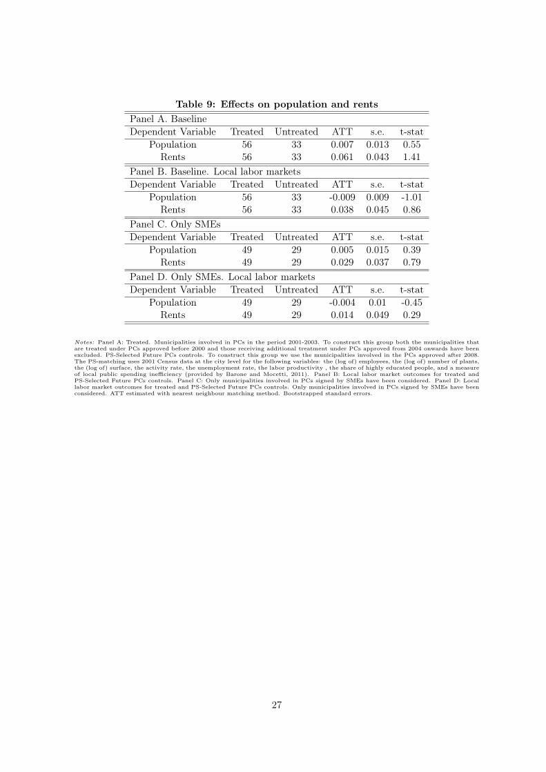
Table 9: Effects on population and rentsPanel A. BaselineDependent Variable Treated Untreated ATT s.e. t-stat

Population 56 33 0.007 0.013 0.55Rents 56 33 0.061 0.043 1.41

Panel B. Baseline. Local labor marketsDependent Variable Treated Untreated ATT s.e. t-stat

Population 56 33 -0.009 0.009 -1.01Rents 56 33 0.038 0.045 0.86

Panel C. Only SMEsDependent Variable Treated Untreated ATT s.e. t-stat

Population 49 29 0.005 0.015 0.39Rents 49 29 0.029 0.037 0.79

Panel D. Only SMEs. Local labor marketsDependent Variable Treated Untreated ATT s.e. t-stat

Population 49 29 -0.004 0.01 -0.45Rents 49 29 0.014 0.049 0.29

Notes: Panel A: Treated. Municipalities involved in PCs in the period 2001-2003. To construct this group both the municipalities thatare treated under PCs approved before 2000 and those receiving additional treatment under PCs approved from 2004 onwards have beenexcluded. PS-Selected Future PCs controls. To construct this group we use the municipalities involved in the PCs approved after 2008.The PS-matching uses 2001 Census data at the city level for the following variables: the (log of) employees, the (log of) number of plants,the (log of) surface, the activity rate, the unemployment rate, the labor productivity , the share of highly educated people, and a measureof local public spending inefficiency (provided by Barone and Mocetti, 2011). Panel B: Local labor market outcomes for treated andPS-Selected Future PCs controls. Panel C: Only municipalities involved in PCs signed by SMEs have been considered. Panel D: Locallabor market outcomes for treated and PS-Selected Future PCs controls. Only municipalities involved in PCs signed by SMEs have beenconsidered. ATT estimated with nearest neighbour matching method. Bootstrapped standard errors.

27

Appendix

Table A: PCs implemented since their emergence in 1986Name of the PC Date of Number of Located in Sector Planned Share of

approval municipalities the South investments public fundsFIAT1 13/04/1988 21 YES Manufacturing 1829.45 0.55OLIVETTI 28/07/1988 6 YES Informatics 0.40 0.75IRI 17/05/1989 14 YES Manufacturing 747.26 0.56TEXAS1 07/11/1989 3 YES Informatics 870.80 0.56GTC 24/04/1990 1 YES Manufacturing 99.89 0.46BULL HN 10/05/1990 1 YES Informatics 82.72 0.63ENI 03/04/1991 5 YES Energy 0.69 0.36IBM 23/10/1991 3 YES Informatics 0.03 0.75FIAT2 05/11/1991 9 YES Manufacturing 3232.92 0.45SNIA BDP 04/02/1992 6 YES Manufacturing 789.50 0.48PIAGGIO 26/02/1992 3 YES Manufacturing 0.14 0.32BARILLA 14/04/1992 4 YES Manufacturing 444.10 0.42SARAS1 19/06/1995 2 YES Manufacturing 366.53 0.32TARI 23/06/1995 1 YES Manufacturing 54.31 0.63ACM 27/06/1995 9 YES Manufacturing 0.29 0.55COMPLASINT 27/06/1995 1 YES Manufacturing 0.05 0.51NATUZZI 31/10/1996 7 YES Manufacturing 69.77 0.50IPM 06/12/1996 4 YES Manufacturing 73.78 0.65UNICA1 09/04/1997 1 YES Manufacturing 44.28 0.65GETRAG 09/07/1997 1 YES Manufacturing 210.54 0.52SGS THOMSON 09/07/1997 1 YES Manufacturing 305.59 0.56SARAS2 10/10/1997 1 YES Manufacturing 250.42 0.52UNICA2 29/10/1997 1 YES Manufacturing 45.41 0.66NUOVA CONCORDIA 09/01/1998 1 YES Tourism 45.41 0.66TELIT 24/03/1998 2 YES Manufacturing 80.77 0.58EDS 21/10/1999 1 YES Services 20.30 0.58TARANTO CONT. TERM. 13/09/2001 1 YES Manufacturing 41.00 0.55CTM CENTRO TESSILE 04/10/2001 1 YES Manufacturing 78.77 0.61CONSORZIO MADIA DIANA 11/10/2001 1 YES Agro-industry 49.20 0.65LEAR PROMA 17/12/2001 7 YES Manufacturing 55.00 0.40IMPRECO 20/12/2001 2 YES Manufacturing 164.76 0.70TRAPANI TURISMO 21/12/2001 14 YES Tourism 90.12 0.57ATLANTIS 24/12/2001 3 YES Manufacturing 21.18 0.67SAM 23/01/2002 7 YES Manufacturing 52.68 0.667C ITALIA 11/02/2002 1 YES Services 8.24 0.49BOSCH 13/02/2002 1 YES Manufacturing 198.29 0.46ATITECH 22/04/2002 1 YES Services 23.53 0.40SANDALIA 23/04/2002 4 YES Tourism 87.66 0.44DISTRETTO ELETTRODOMESTICO 24/05/2002 12 YES Manufacturing 109.32 0.45CONSORZIO ALISAN 29/05/2002 5 YES Agro-industry 87.15 0.66SARAS3 10/06/2002 3 YES Manufacturing 65.93 0.46CONSORZIO LATTE 09/12/2002 18 YES Agro-industry 100.00 0.51EDISON 09/12/2002 1 NO Manufacturing 615.72 0.11IVECO SPA 09/12/2002 1 YES Manufacturing 265.61 0.46APREAMARE 16/12/2002 1 YES Manufacturing 49.90 0.47BIOMASSE ITALIA 16/12/2002 2 YES Manufacturing 130.70 0.38EUROSVILUPPO 16/12/2002 1 YES Agro-industry 49.05 0.54PROCAL 16/12/2002 6 YES Manufacturing 57.68 0.70AGROFUTURO 11/01/2003 13 YES Agro-industry 111.31 0.63FELANDINA 05/03/2003 1 YES Manufacturing 109.19 0.53NUOVA BIOZENIT 05/03/2003 1 YES Agro-industry 52.48 0.33CONSORZIO SIKELIA 05/06/2003 20 YES Agro-industry 96.80 0.52PIRELLI 05/06/2003 1 YES Manufacturing 167.39 0.44COSTA D’ORO 31/07/2003 3 YES Tourism 93.62 0.54POLO FLORICOLO 31/07/2003 1 YES Agriculture 48.41 0.40SERRAMARINA 31/07/2003 1 YES Agriculture 27.09 0.72MARCONI MOBILE ACCESS 18/12/2003 1 YES Manufacturing 58.23 0.28CONS. SVILUPPO INDUSTRIALE SCARL 13/07/2004 1 YES Food-industry 90.98 0.51AREA AQUILANA 22/07/2004 1 YES Manufacturing 80.03 0.28GRUPPO FIAT 22/07/2004 3 YES Manufacturing 1251.25 0.12POLO TURISTICO TERMALE 29/07/2004 1 YES Tourism 37.49 0.65

28

Appendix (continue)

Table A (continue): PCs implemented since their emergence in 1986 (continue)Name of the PC Date of Number of Located in Sector Planned Share of

approval municipalities the South investments public fundsCONS. NAUTICO POLIFUNZIONALE 28/02/2005 2 YES Manufacturing 106.24 0.52CONSORZIO AQUAM 14/07/2005 1 NO Agro-industry 46.63 0.25CONS. SVIL. AGROIND. PIEMONTESE 14/07/2005 15 NO Agro-industry 27.30 0.39ALL COOP 28/07/2005 1 YES Agro-industry 27.30 0.39COLACEM 19/02/2006 1 YES Manufacturing 49.80 0.38COPRIT 19/02/2006 4 YES Tourism 102.99 0.61FIAT POWERTRAIN 19/02/2006 1 NO Manufacturing 647.60 0.13GRUPPO FIAT2 19/02/2006 4 YES Manufacturing 43.45 0.24CONSORZIO BSI 27/03/2006 1 YES Agro-industry 61.80 0.50SVILUPPO ITALIA TURISMO 27/03/2006 6 YES Tourism 199.26 0.39TIRRENO SVILUPPO 27/03/2006 11 YES Tourism 45.50 0.48CONSORZIO ALIM 04/05/2006 7 YES Agro-industry 28.97 0.48EQUIPOLYMERS 04/05/2006 1 YES Chemistry 89.99 0.40SEVEL SPA 04/05/2006 1 YES Manufacturing 455.63 0.09SICILIA GOLF RESORT 06/10/2006 2 YES Tourism 97.22 0.43CONSORZIO TUSCANIA 12/01/2007 9 NO Tourism 168.61 0.29CONFLAJ 17/07/2007 5 YES Tourism 53.45 0.36VIDEOCOLOR 25/07/2007 1 NO Manufacturing 274.12 0.16ST MICROELECTRONICS 26/07/2007 1 YES Electronics 1700.00 0.26PAUSANIA 05/09/2007 4 YES Tourism 48.29 0.48MOLISE AGROALIMENTARE 27/09/2007 8 YES Agro-industry 54.96 0.44LA LODIGIANA 04/10/2007 3 NO Agrizootech. 24.30 0.33FIORIFRUTTI 18/03/2008 19 NO Agro-industry 45.87 0.38CONSORZIO CREO 15/04/2008 3 YES Chemistry 32.28 0.43EURALLUMINA 09/05/2008 1 YES Manufacturing 113.67 0.24TROMBINI 29/05/2008 1 NO Agriculture 30.15 0.26POLO TECNOL. CAMPANIA NORD 11/07/2008 1 YES Manufacturing 41.20 0.48CONS. AGROIND. AREE SVANT. PIEM. 24/07/2008 34 NO Agro-industry 117.39 0.32CONS. SVIL. INDUSTR. PIEMONTE 24/07/2008 15 NO Agro-industry 32.56 0.23CONS. TURISTICO SICILIANO 17/09/2008 7 YES Tourism 48.47 0.49MEDITERRANEO VILLAGES 16/10/2008 5 YES Tourism 104.73 0.30CONS. AGROALIM. BASSO FERRARESE 26/11/2008 6 NO Agro-industry 75.33 0.29CONS. CITTÀ DEL LIBRO 26/11/2008 1 YES Publishing 37.20 0.50TECNESUD 26/11/2008 2 YES ICT 62.40 0.60CREA 27/01/2009 3 YES Chemistry 33.63 0.35SELEX COMMUNICATIONS 12/03/2009 2 NO Communication 93.80 0.30CONS. SVIL. INT. SIST. AGROAL. PIEM. 14/09/2009 4 NO Agro-industry 28.50 0.29SVILUPPO TURIST. GOLFO NAPOLI 24/09/2009 3 YES Tourism 63.40 0.39MADE IN ITALY 03/08/2010 10 NO Vitivinicole 63.45 0.29SAM II 03/08/2010 7 YES Manufacturing 50.62 0.40AGROERICINO SCPA to be approved 9 YES Tourism 46.93 0.50ALIMENTA to be approved 1 YES Agro-industry 40.00 0.38ANTICHE TRADIZIONI PUGLIESI to be approved 8 YES Agro-industry 31.99 0.37GENESIS to be approved 1 YES Manufacturing 77.66 0.48GRUPPO CIT to be approved 3 YES Tourism 194.56 0.48HIPPONIUM BIOMED to be approved 1 YES Manufacturing 63.98 0.35INEOS VINYLS ITALIA to be approved 2 YES Chemistry 44.87 0.37OROMARE to be approved 1 YES Manufacturing 50.00 0.40PICENO CONSID to be approved 5 NO Tourism 40.12 0.16PICENO CONSID II to be approved 7 NO Agro-industry 25.88 0.28PICENO CONSID III to be approved 9 NO Manufacturing 60.66 0.14PROGETTO PORTO NAPOLI to be approved 1 YES Tourism 186.53 0.38PROKEMIA to be approved 2 YES Manufacturing 124.53 0.35RIVIERA DEI GELSOMINI to be approved 10 YES Tourism 78.30 0.55SERRAMARINA ADDENDUM to be approved 1 YES Agric.&Tourism 32.64 0.47SOCIETÀ CONS. MELILLI GROUP to be approved 1 YES Agro-industry 87.80 0.58SPAS to be approved 3 YES Ortho/Floricult. 125.02 0.39STT LA TERRA DEL BENESSERE to be approved 5 YES Tourism 84.52 0.45SVILUPPO SICILIA to be approved 16 YES Agro-industry 49.05 0.54ULIVETI DEL SOLE to be approved 16 YES Tourism 50.65 0.44

29

local development that money can’t buy: italy’s contratti ... · local development that money...

Documents