local and global scaling reduce hubs in...

Journal of Machine Learning Research 13 (2012) 2871-2902 Submitted 8/11; Revised 6/12; Published 10/12

Local and Global Scaling Reduce Hubs in Space

Dominik Schnitzer DOMINIK [email protected]

Arthur Flexer [email protected]

Austrian Research Institute for Artificial Intelligence (OFAI)Freyung 6/6, 1010 Vienna, Austria

Markus Schedl [email protected]

Gerhard Widmer [email protected]

Department of Computational PerceptionJohannes Kepler UniversityAltenbergerstraße 69, 4040 Linz, Austria

Editor: Gert Lanckriet

Abstract‘Hubness’ has recently been identified as a general problem of high dimensional data spaces, man-ifesting itself in the emergence of objects, so-called hubs, which tend to be among thek nearestneighbors of a large number of data items. As a consequence many nearest neighbor relations inthe distance space are asymmetric, that is, objecty is amongst the nearest neighbors ofx but notvice versa. The work presented here discusses two classes ofmethods that try to symmetrize near-est neighbor relations and investigates to what extent theycan mitigate the negative effects of hubs.We evaluate local distance scaling and propose a global variant which has the advantage of beingeasy to approximate for large data sets and of having a probabilistic interpretation. Both local andglobal approaches are shown to be effective especially for high-dimensional data sets, which areaffected by high hubness. Both methods lead to a strong decrease of hubness in these data sets,while at the same time improving properties like classification accuracy. We evaluate the methodson a large number of public machine learning data sets and synthetic data. Finally we present areal-world application where we are able to achieve significantly higher retrieval quality.

Keywords: local and global scaling, shared near neighbors, hubness, classification, curse ofdimensionality, nearest neighbor relation

1. Introduction

In a recent publication in this journal, Radovanovic et al. (2010) describe the so-called ‘hubness’phenomenon and explore it as a general problem of machine learning in high-dimensional dataspaces. Hubs are data points which keep appearing unwontedly often asnearest neighbors of alarge number of other data points. This effect is particularly problematic in algorithms for similaritysearch (for example, similarity-based recommenders), as the same similar objects are found overand over again and other objects are never recommended. The effect has been shown to be a naturalconsequence of high dimensionality and as such is yet another aspect ofthe curse of dimensionality(Bellman, 1961).

A direct consequence of the presence of hubs is that a large number ofnearest neighbor rela-tions in the distance space are asymmetric, that is, objecty is amongst the nearest neighbors ofxbut not vice versa. A hub is by definition the nearest neighbor of a largenumber of objects, but

c©2012 Dominik Schnitzer, Arthur Flexer, Markus Schedl and Gerhard Widmer.

SCHNITZER, FLEXER, SCHEDL AND WIDMER

these objects cannot possibly all be the nearest neighbor of the hub. This observation connectsthe hub problem to methods that attempt to symmetrize nearest neighbor relations, such as ‘sharednear neighbors’ (Jarvis and Patrick, 1973) and ‘local scaling’ (Zelnik-Manor and Perona, 2005).While these methods require knowledge of the local neighborhood of every data point, we proposea global variant that combines the idea of ‘shared near neighbor’ approaches with a transformationof distances to nearest neighbor ‘probabilities’ to define a concept we call Mutual Proximity. Theapproach is unsupervised and transforms an arbitrary distance function to a probabilistic similarity(distance) measure. Contrary to the local variants, this new approach lends itself to fast approxima-tion for very large data bases and enables easy combination of multiple distance spaces due to itsprobabilistic nature.

In experiments with a large number of public machine learning databases we show that bothlocal and global scaling methods lead to: (i) a significant decrease of hubness, (ii) an increase ofk-nearest neighbor classification accuracy, and (iii) a strengthening of the pairwise class stability of thenearest neighbors. To demonstrate the practical relevance, we apply our global scaling algorithmto a real-world music recommendation system and show that doing so significantly improves theretrieval quality.

To permit other researchers to reproduce the results of this paper, all databases and the mainevaluation scripts used in this work have been made publicly available.1

2. Related Work

The starting point for our investigations is a field where the existence of hubs has been well doc-umented and established, namely, Music Information Retrieval (MIR). One of the central notionsin MIR is that of music similarity. Proper modeling of music similarity is at the heart of many ap-plications involving the automatic organization and processing of music data bases. In Aucouturierand Pachet (2004), hub songs were defined as songs which are, according to an audio similarityfunction, similar to very many other songs and therefore keep appearing unwontedly often in rec-ommendation lists, preventing other songs from being recommended at all. Such songs that do notappear in any recommendation list have been termed ‘orphans’. Similar observations about falsepositives in music recommendation that are not perceptually meaningful havebeen made elsewhere(Pampalk et al., 2003; Flexer et al., 2010; Karydis et al., 2010). The existence of the hub problemhas also been reported for music recommendation based on collaborative filtering instead of audiocontent analysis (Celma, 2008). Similar effects have been observed in image (Doddington et al.,1998; Hicklin et al., 2005) and text retrieval (Radovanovic et al., 2010), making this phenomenon ageneral problem in multimedia retrieval and recommendation.

In the MIR literature, Berenzweig (2007) first suspected a connection between the hub problemand the high dimensionality of the feature space. The hub problem was seenas a direct result ofthe curse of dimensionality (Bellman, 1961), a term that refers to a number ofchallenges related tothe high dimensionality of data spaces. Radovanovic et al. (2010) were able to provide more insightby linking the hub problem to the property ofconcentration(François et al., 2007) which occurs asa natural consequence of high dimensionality. Concentration is the surprising characteristic of allpoints in a high dimensional space to be at almost the same distance to all other points in that space.It is usually measured as a ratio between some measure of spread and magnitude. For example, theratio between the standard deviation of all distances to an arbitrary reference point and the mean of

1. Databases and scripts can be found athttp://www.ofai.at/~dominik.schnitzer/mp.

2872

LOCAL AND GLOBAL SCALING REDUCE HUBS IN SPACE

these distances. If this ratio converges to zero as the dimensionality goes to infinity, the distances aresaid to concentrate. For example, in the case of the Euclidean distance and growing dimensionality,the standard deviation of distances converges to a constant while the mean keeps growing. Thus theratio converges to zero and the distances are said to concentrate.

The effect of distance concentration has been studied for Euclidean spaces and otherℓp norms(Aggarwal et al., 2001; François et al., 2007). Radovanovic et al. (2010) presented the argument thatin the finite case, due to this phenomenon some points are expected to be closerto the data-set meanthan other points and are at the same time closer, on average, to all other points. Such points closerto the data-set mean have a high probability of being hubs, that is, of appearing in nearest neighborlists of many other points. Points which are further away from that mean havea high probability ofbeing ‘orphans’, that is, never appearing in any nearest neighbor list.

Nearest neighbor search is an essential method in many areas of computerscience, such as pat-tern recognition, multimedia search, vector compression, computational statistics and data mining(Shakhnarovich et al., 2006) and, of course, information retrieval and recommendation. It is a welldefined task: given an objectx, find the most similar object in a collection of related objects. In thecase of recommendation, thek most similar objects are retrieved withk<< n (n being the numberof all objects in the data base). Since hubs appear in very many nearest neighbor lists, they tendto render many nearest neighbor relations asymmetric, that is, a huby is the nearest neighbor ofx,but the nearest neighbor of the huby is another pointa (a 6= x). This is because hubs are nearestneighbors to very many data points but onlyk data points can be nearest neighbors to a hub sincethe size of a nearest neighbor list is fixed. This behavior is especially problematic in classificationor clustering ifx andy belong to the same class buta does not, violating what Bennett et al. (1999)called thepairwise stabilityof clusters. Radovanovic et al. (2010) coined the termbad hubsforpoints that show a disagreement of class information for the majority of data points they are nearestneighbors to. Figure 1 illustrates the effect: althougha is, in terms of the distance measure, thecorrect answer to the nearest neighbor query fory, it may be beneficial to use a distance measurethat enforces symmetric nearest neighbors. Thus a small distance between two objects should bereturned only if their nearest neighbors concur.

This links the hub problem to ‘shared near neighbor’ (SNN) approaches, which try to sym-metrize nearest neighbor relations. The first work to use common near neighbor information datesback to the 1970s. Jarvis and Patrick (1973) proposed a ‘shared near neighbor’ similarity measureto improve the clustering of ‘non-globular’ clusters. As the name suggests,the shared near neighbor(SNN) similarity is based on computing the overlap between thek nearest neighbors of two objects.Shared near neighbor similarity was also used by Ertöz et al. (2003) to find the most representativeitems in a set of objects. Pohle et al. (2006) define a related similarity measure based on the rank ofnearest neighbors. They call their method ‘proximity verification’ and useit to enhance audio sim-ilarity search. Jin et al. (2006) use the reverse nearest neighbor (RNN) relation to define a generalmeasure for outlier detection.

Related to SNN approaches are local scaling methods, which use local neighborhood informa-tion to rescale distances between data points. The intention is to find specific scaling parameters foreach point, to be used to tune the pairwise distances in order to account fordifferent local densities(scales) of the neighborhoods. Local scaling in this sense was first introduced as part of a spectralclustering method by Zelnik-Manor and Perona (2005). It transforms arbitrary distances using thedistance between objectx and itsk’th nearest neighbor (see Section 3.1 below). In the context of im-age retrieval, Jegou et al. (2010) describe a related method called ‘contextual dissimilarity measure’

2873


��

(a) Original nearest neighbor rela-tions

��

(b) Desired nearest neighbor rela-tions

Figure 1: Schematic plot of two classes (black/white filled circles). Each circle has its nearestneighbor marked with an arrow: (a) violates thepairwise stabilityclustering assumption,(b) fulfills the assumption. In many classification and retrieval scenarios, (b) would bethe desired nearest neighbor relation for the data set.

(CDM) and show that it reduces the error rates of the retrieval algorithmsignificantly, observingthat “the neighborhood symmetry rate increases”, while at the same time “the percentage of neverseen images decreases”, and in addition that “the most frequent image is returned 54 times in thefirst 10 positions with the CDM, against 1062 times using the standard L1 distance”. While they donot explicitly make reference to the notion of hubs, their observations indicate the potential of localdistance scaling to mitigate hub-related problems.

3. Scaling Methods

In the previous section we have seen that (i) the emergence of hubs leadsto asymmetric nearestneighbor relations and that (ii) literature already contains hints that local scaling methods seem toimprove the situation. However a detailed analysis of these facts and a systematic connection to theinvestigations of Radovanovic et al. (2010) has not yet been done.

In what follows we review the local scaling methods and introduce a new global variant, whichis also very simple to use. Due to its probabilistic modeling it possesses certain advantages over thelocal variant. Both methods are evaluated in regard to their effects on hubness in Section 4.

All the methods described here assume an underlying distance (divergence) measure with thefollowing properties:

Definition 1 Given a non-empty set M with n objects, each element mx ∈ M is assigned an indexx= 1. . .n. We define a divergence measure d: M×M →R satisfying the condition of non-negativityin its distances:

2874


• non-negativity: d(mx,my)≥ 0, mx,my ∈ M,

Individual objectsmx ∈ M are referenced in the text by their indexx. The distance between twoobjectsx andy is denoted asdx,y.

3.1 Local Scaling

Local scaling (Zelnik-Manor and Perona, 2005) transforms arbitrarydistances to so-calledaffinities(that is, similarities) according to:

LS(dx,y) = exp

(

− dx,y2

σx σy

)

, (1)

whereσx denotes the distance between objectx and itsk’th nearest neighbor.LS(dx,y) tends tomake neighborhood relations more symmetric by including local distance statisticsof both datapoints x and y in the scaling. The exponent in Equation 1 can be rewritten asdx,y

2/σx σy =(dx,y/σx)(dx,y/σy): only when both parts in this product are small will the locally scaled similarityLS(dx,y) be high. That is,x andy will be considered close neighbors only if the distancedx,y is smallrelative to both local scalesσx andσy. Jegou et al. (2007) introduce a closely related variant callednon-iterative contextual dissimilarity measure (NICDM). Instead of using the distance to thek’thnearest neighbor to rescale the distances, the average distance of thek nearest neighbors is used.This should return more stable scaling numbers and will therefore be used inall our evaluations.The non-iterative contextual dissimilarity measure (NICDM) transforms distances according to:

NICDM(dx,y) =dx,y√µxµy

,

whereµx denotes the average distance to thek nearest neighbors of objectx. The iterative versionof this algorithm performs the same transformation multiple times until a stopping criterion is met.Since these iterations yield only very minor improvements at the cost of increased computationtime, we used the non-iterative version in our evaluations.

3.2 Global Scaling - Mutual Proximity

In this section we introduce a global scaling method that is based on: (i) transforming a distancebetween pointsx andy into something that can be interpreted as the probability thaty is the closestneighbor tox given the distribution of the distances of all points tox in the data base; and (ii)combining these probabilistic distances fromx to y andy to x via their joint probability. The result isa general unsupervised method to transform arbitrary distance matrices tomatrices of probabilisticmutual proximity(MP). In contrast to local scaling methods, which use the local neighborhoodinformation, MP uses information about all objects—thus the term global scaling.

The general idea of MP is to reinterpret the original distance space so that two objects sharingsimilar nearest neighbors are more closely tied to each other, while two objectswith dissimilarneighborhoods are repelled from each other. This is done by reinterpreting the distance of twoobjects as a mutual proximity in terms of their distribution of distances.

2875


(a) Original space: A tight cluster(gray dots in the center) placed ina loose background cluster (blackdots).

(b) The affinity of two points inthe original space is indicated bythe thickness of the line connectingtwo points.

(c) Affinities after applying MutualProximity to the distances.

Figure 2: The effect of scaling techniques. Objects with similar nearest neighbors are tied togetherclosely, while objects with dissimilar neighbors are repelled.

Figure 2 illustrates the effect of this reinterpretation in an example. The effect which can be seenhere is similar to the intuitive repair of nearest neighbor relation as it was discussed in the beginningin Section 2 (Figure 1).

Figure 2a plots points from two classes on a two dimensional plane. A tight cluster (the graydots in the center) is placed in a loose background cluster (black dots). Figure 2b connects closeneighbors with lines according to a Delaunay triangulation.2 The thickness of the lines shows theaffinity of two neighboring points according to their Euclidean distance. Thethird plot (Figure 2c)plots the affinities after applying MP. It can be clearly seen that points fromthe loose cluster as wellas points from the tight cluster now both have a high intra-class affinity. However, at the clusterborders there is weak affinity and strong separation as points from the tight cluster have differentnearest neighbors than points from the background cluster.

This visible increase in class separation can also be measured in terms of classification rates.Simple two class k-nearest neighbor classification (tight vs. loose cluster)with this artificially gen-erated data yields the following results: In the original space 96.4% of the nearest neighbors (atk= 1) are classified correctly; after applying MP, all (100%) of the nearest neighbors can be classi-fied correctly. Fork= 5 the classification rate increases from 95.2% to 98.8%.

3.2.1 COMPUTING MUTUAL PROXIMITY (MP)

To compute MP, we assume that the distancesdx,i=1..n from an objectx to all other objects in ourcollection follow a certain probability distribution. For example, Casey et al. (2008) and Cai et al.(2007) show that theℓp distances they compute follow a Gamma distribution. Ferencz et al. (2005)used the Gamma distribution to modelℓ2 distances from image regions. Pekalska and Duin (2000)show in general that based on the central limit theorem and if the feature vectors are independent and

2. A Delaunay triangulation ensures that the circumcircle associated with each triangle contains no other point in itsinterior, that is, no lines cross. This restriction is helpful for visualization purposes.

2876


identically distributed (i.i.d.), theirℓ2 distances approximately follow a normal distribution. As realdata is not i.i.d., this can not be assumed. We, however, note that the accuracy of this approximationincreases with increasing intrinsic dimensionality (François et al., 2007).

Under the assumption that all distances in a data set follow a certain distribution, any distancedx,y can now be reinterpreted as the probability ofy being the nearest neighbor ofx, given theirdistancedx,y and the probability distributionP(X). P(X) is defined by the distances ofx to all otherobjects in the collection. In fact the probability that a randomly drawn elementzwill have a distancedx,z > dx,y can then be computed:

P(X > dx,y) = 1−P(X ≤ dx,y) = 1−Fx(dx,y).

Fx denotes the cumulative distribution function (cdf) which is assumed for the distribution ofdistancesdx,i=1..n. This way the probability of an element being a nearest neighbor ofx increaseswith decreasing distance.

For illustration purposes we assume that in our collection the distances are normally distributed.Figure 3a shows a schematic plot of the probability density function (pdf) that was estimated forthe distances of some objectx. The mean distance or expected distance fromx (µx) is in the centerof the density function. Objects with a small distance tox (that is, objects with high similarity inthe original space) find their distance towards the left of the density function. Note that the leftmostpossible distance in this sketch isdx,x = 0.3 Figure 3b plots the probability ofy being the nearestneighbor ofx givendx,y (the gray filled area). The probability increases the smaller the distance tox is, or the farther left its distance is on the x-axis of the pdf.

Note that this reinterpretation naturally leads to asymmetric probabilities for a given distance,as the distance distribution estimated forx may be different from the one estimated fory; x might bethe nearest neighbor ofy but not vice versa. Contrary to the original distances the probabilities nowencode this asymmetric information. This allows for a convenient way to combinethe asymmetricprobabilities into a single expression, expressing the probability ofx being a nearest neighbor ofyand vice versa.

Definition 2 We compute the probability that y is the nearest neighbor of x given P(X) (the pdfdefined by the distances dx,i=1...n) and x is the nearest neighbor of y given P(Y) (the pdf definedby the distances dy,i=1...n), with their joint distribution P(X,Y). The resulting probability is calledMutual Proximity (MP):

MP(dx,y) = P(X > dx,y∩Y > dy,x)

= 1−P(X ≤ dx,y∪Y ≤ dx,y)

= 1− [P(X ≤ dx,y)+P(Y ≤ dy,x)−P(X ≤ dx,y∩Y ≤ dy,x)] .

Figure 4 illustrates MP for the distancedx,y and the joint distance distribution ofX andY,P(X,Y). Each point of the plot refers to an object in the collection and its distance to pointsx andy.The shaded area (II) then defines the probability which is computed by MP.Sectors I+III correspond

3. Strictly speaking, then, the interpretation of this as a normal distribution is incorrect, since distances< 0 are notpossible. However, we find the interpretation useful as a metaphor that helps understand why it makes sense tocombine different views. We will do so in this section.

2877


X ~ N(µx, σ

x)

dx,x

f(dx,i

)

dx,i=1..n

µx

− σx

µx

µx+σ

x

(a) The closer other elements are tox, the more to the left is their distance located onthe x-axis of the density function plot. The leftmost possible observation in the datais the distancedx,x = 0.

X ~ N(µx, σ

x)f(d

x,i)

dx,i=1..n

dx,x

P(X > dx,y

)

dx,y

(b) The shaded area shows the probability thaty is the nearest neighbor ofx basedon the distancedx,y and X. The closery is to x (the smallerdx,y) the higher theprobability.

Figure 3: Schematic plot of the probability density function of a normal distribution which wasestimated from the distancesdx,i=1...n: X ∽ N(µx, σx).

to the probability ofx being the nearest neighbor ofy, IV+III to the probability ofy being a nearestneighbor ofx and III to their joint probability:

II = MP(dx,y) = 1− [(I + III )+(IV + III )− III ].

It is straightforward to compute MP using the empirical distribution, as illustratedin Figure 4.If the number of observations is large enough, we will tend to model the true underlying distributionclosely. Computing MP for a given distancedx,y in a collection ofn objects and using the empirical

2878


�

��

��

��

��

��

�

��

��

Figure 4: Visualizing the Mutual Proximity for the two pointsx, y, and their distancesdx,y, dy,x.

distribution boils down to simply counting the number of objectsj having a distance tox andywhich is greater thandx,y:

MP(dx,y) =

∣

∣

{

j : dx, j > dx,y}

∩{

j : dy, j > dy,x}∣

∣

n.

For distances where the underlying distribution is known, estimating its parameters can bestraightforward. For example, the parameters of normal distributionsN(µ, σ2), or Gamma distri-butionsΓ(k, θ) can be estimated quickly with the sample mean ˆµx and varianceσ2

x of the distancesdx,i=1..n:

Nx ∽ µx =1n

n

∑i=1

dx,i , σ2x =

1n

n

∑i=1

(dx,i − µx)2, (2)

Γx ∽ kx =µ2

x

σ2x, θx =

σ2x

µx.

In our experiments we will generally estimate MP directly from the empirical distribution. In ad-dition we will also evaluate MP with different underlying parametric distance distributions, such asthe Gauss or Gamma distribution (Section 4).

3.2.2 APPROXIMATIONS

The definition of MP (Definition 2) requires estimating a joint distributionP(X,Y) for all distancepairsdx,y, which is usually expensive to compute. On the other hand, if independence could be as-sumed between distributionsP(X) andP(Y), the computation of MP would simplify in accordancewith the product rule:

MPI (dx,y) = P(X > dx,y) ·P(Y > dy,x). (3)

2879


We will show in our experiments that assuming independence in the computation of MP does notaffect the results in an adverse way (Section 4).

In the base case where MP is computed from the empirical distribution as well asall other vari-ants presented so far, the computational cost of computing MP grows quadratically with the sizeof the data set as all methods require the full distance matrix (that is, all possible distances) to becomputed. To circumvent this, we propose to estimate the distribution parametersby randomly se-lecting a small fraction of objects to compute the mean and standard deviation of distances for eachobject using only the subset of objects. We denote MP where the parameters have been estimatedby sampling from the collection with MPS. The parameterSspecifies how many objects have beenrandomly sampled. The appropriate sample size is naturally dependent on theunderlying distri-bution. However if a normal distribution may be assumed, a sample size as small as S= 30 willalready yield stable results for MP.

The difference to the original estimation of the parameters in Equation 2 is that only a smallfraction of distances (S×n) needs to be computed, which, for constantS, reduces the complexityfrom quadratic to linear inn. This is also more efficient than local scaling, where the actual nearestneighbors of pointsx andy need to be identified. While local scaling methods can of course be usedwith fast nearest neighbor search algorithms indexing the high dimensionalspaces, the complexityis far higher than randomly sampling only a constant number of distances.

Experimental verification that these approximations of the original idea are still valid will bepresented in Section 4.

3.2.3 LINEAR COMBINATION OF DISTANCE MEASURES

Another nice property of MP which can be useful in some contexts is that MPyields[0,1]-normalizedsimilarities. Thus, the MP transformation can easily be used to linearly combine multiple differentdistance measuresd1 andd2 for some combination weightsω1,2:

d = ω1MP(d1)+ω2MP(d2).

Similar to a global zero-mean unit-variance normalization, each object’s distances are also stan-dardized by their respective mean and standard deviation. Thus, no distance measure can dominatethe other in this combination. This property is useful in scenarios where multipledifferent dis-tance measures (describing different aspects of a phenomenon) needto be linearly combined. Areal-world example where this is necessary is presented in Section 5.

4. Evaluation

To investigate the effects of using local neighborhood scaling methods andMP, we first evaluate themethods on 30 public machine learning data sets. Each data set is characterized by the followingparameters: name/origin, number of classes, size/number of itemsn and data dimensionalityd.For each data set we evaluate the original distance space and compare it tothe distances that aregenerated by the local scaling method and by MP.

After showing the impact of the scaling methods in regard to the hub problem onreal data setsin the first set of experiments, a second series of experiments investigatesthe effects of the methodsmore deeply. Synthetic as well as real data is used.

2880


4.1 Benchmarks

To quantify the impact of the two methods, a number of properties and quality measures are com-puted for the original and the new distances. The characteristics which wecompute for each dataset are:

4.1.1 LEAVE-ONE-OUT k-NEARESTNEIGHBOR CLASSIFICATION ACCURACY (Ck)

We report thek-nearest neighbor (kNN) classification accuracy using leave-one-out cross-validation,where classification is performed via a majority vote among thek nearest neighbors, with the classof the nearest neighbor used for breaking ties. We denote thek-NN accuracy asCk. In the contextof a retrieval problem, higher values would indicate better retrieval quality.4

To test for statistical significance differences in classification accuracybetween two algorithms,we use McNemar’s test (see Salzberg, 1997 and Dietterich, 1998 for a discussion of using this testin conjunction with leave-one-out classification). When comparing two algorithms A and B, onlyclassification instances where A and B disagree are being analyzed. More specifically, it is testedwhether the number of times that A classifies correctly and B does not is significantly different fromthe number of times B classifies correctly and A does not.

4.1.2 K-OCCURRENCE(Nk(x))

Defines thek-occurrences of objectx, that is, the number of timesx occurs in thek nearest neighborlists of all other objects in the collection.

4.1.3 HUBNESS(Sk)

We also compute thehubnessof the distance space of each collection according to Radovanovicet al. (2010). Hubness is defined as the skewness of the distribution ofk-occurrencesNk:

Sk =E[

(Nk−µNk)3]

σ3Nk

.

Positive skewness indicates high hubness, negative values low hubness.

4. To clarify the cross-validation (CV) process: We first compute the distance matrix for the entire data set ofn instances,transform this into an MP matrix, and then perform leave-one-out cross-validation on the data set ofn instances, ineach iterationi using one of then instances (xi) as a test case to be classified by its nearest neighbors among theremainingn− 1 instances. It might seem that the ‘test’ examplexi plays an undue role in this process, havingcontributed to the the normalization of the distance matrix before being used as a ‘new’ test case. However, in a‘real’ classification scenario, where we would have a fixed training setXn−1 (consisting ofn−1 instances) and arepresented with a new objectxi to classify (not contained inXn−1), we would also first have to compute the fulldistance matrix overXn−1∪{xi} in order to then be able to compute MP over this matrix. (That is because MP needsinformation about all distances to and fromxi .)

The result of this would be exactly the MP matrix we compute beforehand in our cross-validation process—andit is the exact same matrix for all other ‘test’ instances fromX. Thus, it is legitimate to compute this once and forall before the CV. On the other hand, the above means that using MP in a ‘real’ classification scenario is expensive,because before being able to classify a new instance, first a complete distance and MP matrix have to be computed.What makes this process feasible in practice is the MP approximation MPS described in Section 3.2.2.

2881


4.1.4 GOODMAN-KRUSKAL INDEX (IGK)

The Goodman-Kruskal Index (Günter and Bunke, 2003) is a clusteringquality measure that relatesthe number ofconcordant(Qc) anddiscordant(Qd) tuples (di, j , dk,l ) of a distance matrix.

• A tuple is concordant if its itemsi, j are from the same class, itemsk, l are from differentclasses anddi, j < dk,l .

• A tuple is discordant if its itemsi, j are from the same class, itemsk, l are from differentclasses anddi, j > dk,l .

• A tuple is not counted if it is neither concordant nor discordant, that is, ifdi, j = dk,l .

The Goodman-Kruskal Index (IGK) is defined as:

IGK =Qc−Qd

Qc+Qd.

IGK is bounded to the interval[−1,1], and the higherIGK, the more concordant and fewer dis-cordant quadruples are present in the data set. Thus a large index value indicates a good clustering(in terms ofpairwise stability—see Section 2).

Other indices to compare clustering algorithms like the classic Dunn’s Index orDavies-BouldinIndex (Bezdek and Pal, 1998) cannot be used here as their values donot allow a comparison acrossdifferent distance measures.

4.1.5 INTRINSIC DIMENSIONALITY (dmle)

To further characterize each data set we compute an estimate of the intrinsic dimensionality ofthe feature spaces. Whereas the embedding dimension is the actual number of dimensions of afeature space, the intrinsic dimension is the—often much smaller—number of dimensions necessaryto represent a data set without loss of information. It has also been demonstrated that hubnessdepends on the intrinsic rather than embedding dimensionality (Radovanovic et al., 2010). We usethe maximum likelihood estimator proposed by Levina and Bickel (2005), whichwas also used byRadovanovic et al. (2010) to characterize the data sets.

4.1.6 PERCENTAGE OF SYMMETRIC NEIGHBORHOOD RELATIONS

We call a nearest neighbor relation between two pointsx andy ‘symmetric’ if the following holds:objectx is a nearest neighbor ofy if and only if y is also the nearest neighbor ofx. As both exam-ined methods aim at symmetrizing neighborhood relations, we report the percentage of symmetricrelations at different neighborhood sizesk.

4.2 Public Machine Learning Data Sets

We evaluate the proposed method by applying it to 30 different public machinelearning data sets.The data sets include problems from the general machine learning field, andthe bio-medical, image,text and music retrieval domains. We use the following data sets:

2882


• The UCI Machine Learning Repository (UCI, see Frank and Asuncion, 2010) data sets:arcene, gisette, mfeat-pixels/karhunen/factors, dexter, mini-newsgroups, dorothea, reuters-transcribed.5

• The Kent Ridge bio-medical data sets (KR): amlall, lungcancerandovarian-61902.6

• The LibSVM data sets (LibSVM, see Chang and Lin, 2001):australian, diabetes, germannumbers, liver-disorders, breast-cancer, duke (train), heart, sonar, colon-cancer, fourclass,ionosphere, splice.7

• The Music Information Retrieval Evaluation eXchange (MIREX) data sets (Mirex, see Downie,2008):ballroomandismir2004.8

• Two music artist web pages and tweets data sets (CP, see Schedl, 2010):c1ka-twitterandc224a-web.9

For the general machine learning data sets from the statistical or biological domains no featureextraction is necessary. The feature vectors can be downloaded directly from the respective repos-itories. These general machine learning data sets use the standard Euclidean distance (denoted asℓ2) as similarity measure.

The text retrieval data sets (reuters-transcribed, c224a-web, movie-reviews, dexter,mini-newsgroups, c1ka-twitter) need to be preprocessed before evaluating them.10 To this end weemploy stop-word removal and stemming. They are transformed into the bag-of-words representa-tion, and standardt f · id f (term frequency· inverse document frequency) weights are computed (seefor example Baeza-Yates and Ribeiro-Neto, 1999). The word vectors are normalized to the averagedocument length. Individual document vectors are compared with the cosine distance (denoted ascos).

For the image retrieval data set (corel) normalized color histograms are computed as features.They show reasonable classification performance despite their simplicity, asChapelle et al. (1999)show. The three 64-dimensional color histograms are concatenated into a single vector and com-pared using the Euclidean distance (ℓ2).

To extract the features for the two music information retrieval data sets (ismir2004, ballroom) weuse a standard algorithm from Mandel and Ellis (2005) which computes MelFrequency CepstrumCoefficients (Logan, 2000) and models each object as a multivariate normal distribution over these.Objects (models) are compared using the symmetrized Kullback-Leibler divergence (denoted asskl).

4.3 Results

In the following experiments we compute all previously introduced benchmarknumbers for theoriginal data and the distance spaces after applying the scaling methods (NICDM, MP). We use MPas defined in Section 3.2 and model the distance distributions with the empirical distribution.

5. The UCI Repository can be found athttp://archive.ics.uci.edu/ml/.6. The Kent Ridge data sets can be found athttp://datam.i2r.a-star.edu.sg/datasets/krbd/.7. LibSVM can be found athttp://www.csie.ntu.edu.tw/~cjlin/libsvmtools/datasets/.8. The MIREX data sets can be found athttp://www.music-ir.org/mirex.9. These data sets can be found athttp://www.cp.jku.at/people/schedl/datasets.html.

10. Setc1ka-twitterequalsc3ka-twitterfrom CP, omitting artists classified as ‘rock’ to balance the data.

2883


Tables 1 and 2 show the results of the evaluations conducted on the 30 previously introducedpublic data sets. The collections have very diverse properties. There are collections likefourclassor liver-disorderswith very low dimensionality (d = 2 andd = 6), as well as data sets with veryhigh embedding dimensionality, such asdorothea(d = 100000) orc1ka-twitter(d = 49820). Re-lated to that, columndmle lists the intrinsic dimensionality according to the maximum likelihoodestimator. Using the intrinsic dimensionality estimate we can see that there are data sets where thedata is originally represented using high-dimensional feature vectors, although the data’s intrinsicdimensionality is quite low. For example theovarian_61902data set has an embedding dimensionof d = 15154 but its estimated intrinsic dimension is onlydmle= 9.

The evaluation results in Tables 1 and 2 are sorted by the hubnessSk=5 of the original distancespace (printed in bold). In subsequent plots individual collections are referenced by their numbersas given in Tables 1 and 2. The columnsCk=1/Ck=5 show thek-nearest neighbor classification ratesof the collections. The classification rates with the original distances, the local scaling (NICDM)and the global scaling (MP) are documented. For convenience the column+/- shows the differencein classification accuracy, in terms of absolute percentage points, betweenthe original distancesand NICDM/MP. All improvements compared to the original distances are printed in bold. Statis-tically significant differences are marked with an asterisk (McNemar’s test,df = 1, α = .05 errorprobability).

Looking at the tables, a first observation is that very high-dimensional data sets (in terms oftheir intrinsic as well as their embedding dimensionality) also tend to have high hubness. This is inagreement with the results of Radovanovic et al. (2010) and the theory that hubness is a consequenceof high dimensionality.

By looking at the classification rates (columnsCk=1 andCk=5) it can also clearly be observed thatthe higher the hubness and intrinsic dimensionality, the more beneficial, in terms of classificationaccuracy, NICDM and MP. For data sets with high hubness (in the collections we used, a valueabove 1.4 seems to be a limit) the increase in classification rates is notable. ForCk=1, the accuracygain ranges from rather moderate 1 to up to 7−8 percentage points, and in the case ofc1ka-twitteritis 15.9 percentage points for NICDM and 17.1 percentage points for MP. ForCk=5 the trend is evenclearer. Whereas only three changes in accuracy (relative to the original distances) are significantfor data sets with low hubness (Sk=5 ≤ 1.4, data sets 1–17), 34 changes in accuracy are significantfor data sets with high hubness (Sk=5 > 1.4, data sets 18–30). There is no statistically significantnegative change in terms of classification accuracies.

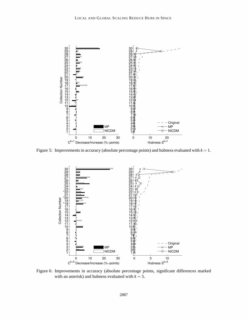
Figures 5 and 6 (left hand sides) present these results in bar plots where the y-axis shows theindex of the data sets (ordered according to hubness as in Tables 1 and 2) and the bars show theincrease or decrease of classification rates. The bar plots also directly show how MP compares toNICDM in terms of classification accuracy fork = 1,5. Generally speaking, results for MP andNICDM are very comparable. As fork = 1, MP and NICDM perform equally well and there isno statistically significant difference between MP and NICDM (McNemar’s test, df = 1, α = .05error probability). Based on the same statistical testing procedure, resultsfor NICDM andk= 5 aresignificantly better than for MP for data sets 18, 20, 22 (marked with asterisks in Figure 6). Thegeneral tendency of both MP and NICDM is comparable in the sense that if there is an improvementcompared to the original distances, it can be seen for both MP and NICDM.

Another observation from the results listed in Tables 1 and 2 is that both NICDM and MPreduce the hubness of the distance space for all data sets to relatively lowvalues. The hubnessSk=5

decreases from an average value of 2.5 (original) to 0.29 (MP) and 0.94(NICDM), indicating a

2884


Name/Src. Cls. n d dmle Dist. Ck=1 +/-Ck=5 +/-

Sk=5 IGK%-pts %-pts

fourclass (sc) 2 862 2 2 ℓ2 100% 100% 0.15 0.221. LibSVM NICDM 100% 0 100% 0 0.06 0.21

MP 100% 0 100% 0 0.04 0.23

arcene 2 100 10 000 399ℓ2 82.0% 75.0% 0.25 0.072. UCI NICDM 81.0% -1.0 77.0% 2.0 -0.27 0.06

MP 80.0% -2.0 81.0% 6.0 0.15 0.10

liver-disorders (sc) 2 345 6 6 ℓ2 62.6% 60.6% 0.39 0.003. UCI NICDM 63.2% 0.6 65.8% *5.2 -0.04 0.03

MP 62.9% 0.3 65.5% *4.9 -0.03 0.01

australian 2 690 14 3 ℓ2 65.5% 68.8% 0.44 0.134. LibSVM NICDM 65.7% 0.2 69.4% 0.6 -0.09 0.14

MP 65.4% -0.1 68.4% -0.4 0.08 0.14

diabetes (sc) 2 768 8 6ℓ2 70.6% 74.1% 0.49 0.205. UCI NICDM 69.8% -0.8 74.1% 0 0.04 0.15

MP 70.3% -0.3 73.2% -0.9 -0.02 0.19

heart (sc) 2 270 13 7 ℓ2 75.6% 80.0% 0.50 0.356. LibSVM NICDM 75.9% 0.3 79.3% -0.7 -0.00 0.27

MP 75.6% 0 80.4% 0.4 0.08 0.39

ovarian-61902 2 253 15 154 10ℓ2 95.3% 93.7% 0.66 0.207. KR NICDM 95.7% 0.4 93.3% -0.4 -0.10 0.19

MP 94.1% -1.2 94.1% 0.4 -0.28 0.19

breast-cancer (sc) 2 683 10 5ℓ2 95.6% 97.4% 0.71 0.898. LibSVM NICDM 95.8% 0.2 97.1% -0.3 0.19 0.42

MP 96.0% 0.4 97.1% -0.3 0.22 0.91

mfeat-factors 10 2 000 216 7ℓ2 95.0% 94.7% 0.79 0.719. UCI NICDM 94.8% -0.2 94.7% 0 0.15 0.76

MP 94.5% -0.5 94.9% 0.2 0.01 0.77

colon-cancer 2 62 2 000 11ℓ2 72.6% 77.4% 0.81 0.1910. LibSVM NICDM 69.4% -3.2 82.3% 4.9 0.08 0.18

MP 67.7% -4.9 82.3% 4.9 -0.11 0.19

ger.num (sc) 2 1 000 24 8ℓ2 67.5% 71.7% 0.81 0.0711. LibSVM NICDM 66.8% -0.7 72.0% 0.3 0.32 0.03

MP 67.6% 0.1 71.4% -0.3 0.11 0.07

amlall 2 72 7 129 32 ℓ2 91.7% 93.1% 0.83 0.3112. KR NICDM 93.1% 1.4 97.2% 4.1 0.56 0.33

MP 88.9% -2.8 91.7% -1.4 -0.01 0.34

mfeat-karhunen 10 2 000 64 15ℓ2 97.4% 97.4% 0.84 0.7613. UCI NICDM 97.2% -0.2 97.6% 0.2 0.27 0.74

MP 97.0% -0.4 97.5% 0.1 0.08 0.79

lungcancer 2 181 12 533 60ℓ2 98.9% 100% 1.07 0.5614. KR NICDM 99.4% 0.5 98.9% -1.1 0.31 0.50

MP 98.3% -0.6 97.8% -2.2 0.01 0.56

c224a-web 14 224 1 244 41 cos 86.2% 89.3% 1.09 0.7915. CP NICDM 87.9% 1.7 92.4% *3.1 0.42 0.89

MP 88.4% 2.2 92.4% 3.1 0.22 0.89

Table 1: Evaluation results ordered by ascending hubness (Sk=5) of the original distance space.This table reports data sets with small hubness. Each evaluated data set (Name/Src) isdescribed by its number of classes (Cls.), its size (n), its extrinsic (d) and intrinsic (dmle)data dimension and the distance measure used (Dist). ColumnsCk report the classificationaccuracies at a givenk, the respective adjacent column+/- the difference in classificationaccuracy between the original distances and NICDM/MP (in percentage points), columnIGK the Goodman-Kruskal Index. See Section 4.1 for an explanation of the individualbenchmarks.

2885


Name/Src. Cls. n d dmle Dist. Ck=1 +/-Ck=5 +/-

Sk=5 IGK%-pts %-pts

mfeat-pixels 10 2 000 240 12ℓ2 97.6% 97.7% 1.25 0.7516. UCI NICDM 97.2% -0.4 97.8% 0.1 0.28 0.75

MP 97.2% -0.4 97.5% -0.2 0.13 0.79

duke (train) 2 38 7 129 16 ℓ2 73.7% 68.4% 1.37 0.0217. UCI NICDM 81.6% 7.9 68.4% 0 0.43 0.06

MP 76.3% 2.6 68.4% 0 0.21 0.03

corel1000 10 1 000 192 9 ℓ2 70.7% 65.2% 1.45 0.3318. Corel NICDM 72.9% *2.2 72.0% *6.8 0.39 0.47

MP 71.6% 0.9 70.3% *5.1 0.31 0.50

sonar (sc) 2 208 60 11 ℓ2 87.5% 82.2% 1.54 0.0719. UCI NICDM 87.0% -0.5 87.0% 4.8 0.47 0.08

MP 87.5% 0 84.1% 1.9 0.32 0.08

ionosphere (sc) 2 351 34 13ℓ2 86.9% 85.5% 1.55 0.3120. UCI NICDM 92.3% *5.4 94.3% *8.8 0.28 0.07

MP 91.7% *4.8 89.7% *4.2 0.50 0.27

reuters-transcribed 10 201 2 730 70 cos 44.3% 49.3% 1.61 0.3821. UCI NICDM 45.3% 1.0 52.7% 3.4 0.63 0.32

MP 42.3% -2.0 55.2% *5.9 0.18 0.43

ballroom 8 698 820 12 skl 54.3% 48.1% 2.98 0.1522. Mirex NICDM 57.2% 2.9 51.6% *3.5 1.09 0.20

MP 56.6% 2.3 54.3% *6.2 0.30 0.18

ismir2004 6 729 820 25 skl 80.4% 74.1% 3.20 0.3723. Mirex NICDM 83.8% *3.4 79.0% *4.9 0.77 0.21

MP 83.4% *3.0 77.0% *2.9 0.46 0.45

movie-reviews 2 2 000 10 382 28 cos 71.1% 75.7% 4.07 0.0524. PaBo NICDM 72.0% 0.9 76.0% 0.3 1.22 0.07

MP 71.8% 0.7 76.7% 1.0 0.36 0.07

dexter 2 300 20 000 161 cos 80.3% 80.3% 4.22 0.1025. UCI NICDM 84.3% 4.0 86.0% *5.7 2.02 0.13

MP 83.0% 2.7 90.0% *9.7 0.58 0.13

gisette 2 6 000 5 000 149ℓ2 96.0% 96.3% 4.48 0.1626. UCI NICDM 97.2% *1.2 98.1% *1.8 0.78 0.20

MP 97.4% *1.4 97.9% *1.6 0.34 0.20

splice (sc) 2 1 000 60 27 ℓ2 69.6% 69.4% 4.55 0.0727. LibSVM NICDM 73.3% *3.7 79.3% *9.9 1.51 0.11

MP 72.4% 2.8 77.2% *7.8 0.48 0.10

mini-newsgroups 20 2 000 8 811 188 cos 64.4% 65.6% 5.14 0.4728. UCI NICDM 67.2% *2.8 68.5% *2.9 1.32 0.52

MP 67.7% *3.3 68.4% *2.8 0.60 0.57

dorothea 2 800 100 000 201ℓ2 90.6% 90.2% 12.91 0.2129. UCI NICDM 92.2% 1.6 93.0% *2.8 11.72 0.21

MP 91.5% 0.9 93.1% *2.9 1.66 0.20

c1ka-twitter 17 969 49 820 46 cos 31.9% 26.6% 14.63 0.0830. CP NICDM 47.8% *15.9 53.0% *26.4 2.94 0.33

MP 49.0% *17.1 50.8% *24.2 1.79 0.16

Table 2: Evaluation results ordered by ascending hubness (Sk=5) of the original distance space.This table reports data sets with large hubness. Each evaluated data set (Name/Src) isdescribed by its number of classes (Cls.), its size (n), its extrinsic (d) and intrinsic (dmle)data dimension and the distance measure used (Dist). ColumnsCk report the classificationaccuracies at a givenk, the respective adjacent column+/- the difference in classificationaccuracy between the original distances and NICDM/MP (in percentage points), columnIGK the Goodman-Kruskal Index. See Section 4.1 for an explanation of the individualbenchmarks.

2886


0 10 20 30

123456789

101112131415161718192021222324252627282930

Co

llectio

n N

um

be

r

Ck=1

Decrease/Increase (%−points)

MP

NICDM

0 10 20

123456789

101112131415161718192021222324252627282930

Hubness Sk=1

Original

MP

NICDM

Figure 5: Improvements in accuracy (absolute percentage points) and hubness evaluated withk= 1.

0 10 20 30

123456789

1011121314151617

*1819

*2021

*222324252627282930

Co

llectio

n N

um

be

r

Ck=5


MP

NICDM

0 5 10

123456789

101112131415161718192021222324252627282930

Hubness Sk=5

Original

MP

NICDM

Figure 6: Improvements in accuracy (absolute percentage points, significant differences markedwith an asterisk) and hubness evaluated withk= 5.

2887


1 2 3 4 5 6 7 8 9 10 11 12 13 14 15 16 17 18 19 20 21 22 23 24 25 26 27 28 29 300%

20%

40%

60%

80%

100%

Collection Number

Neig

hborh

ood S

ym

metr

y,

k=

5

Original

MP

NICDM

1 2 3 4 5 6 7 8 9 10 11 12 13 14 15 16 17 18 19 20 21 22 23 24 25 26 27 28 29 300%

20%

40%

60%

80%

100%

Collection Number

Neig

hborh

ood S

ym

metr

y, k=

10%

Original

MP

NICDM

Figure 7: Percentage of symmetric neighborhood relations atk = 5 (above) andk = 10% (below)of the respective collection size.

well balanced distribution of nearest neighbors. The impact of MP and NICDM on the hubness perdata set is plotted in Figures 5 and 6 (right hand sides). It can be seen that both MP and NICDMlead to lower hubness (measured forSk=1,5) compared to the original distances. The effect is morepronounced for data sets having large hubness values according to theoriginal distances.11

11. A notable exception is data set 29 (‘dorothea’) where the reduction inhubness is not so pronounced. This may bedue to the extremely unbalanced distribution of its two classes (9:1).

2888


More positive effects in the distances can also be seen in the increase of concordant (see Sec-tion 4 for the definition) distance quadruples indicated by higher Goodman-Kruskal index values(IGK). This index improves or remains unchanged for 27 out of 30 data sets in the case of using MP.The effect is not so clear for NICDM, which improves the index or leavesit unchanged for only 17out of 30 data sets. The effect of NICDM onIGK is especially unclear for data with low hubness(data sets 1–17).

Finally we also checked whether both MP and NICDM are able to raise the percentage of sym-metric neighborhood relations. Results fork = 5 andk set to 10% of the collection size (denotedby k = 10%) are shown in Figure 7. As can be seen, the symmetry in the nearest neighbors for alldata sets increases with both MP and NICDM. For NICDM there are two cases (data set 13 and 16)where the neighborhood symmetry does not increase. The average percentage of symmetric neigh-borhoods across all data sets fork= 5 is 46% for the original distances, 69% for MP, and 70.8% forNICDM. The numbers fork= 10% are 53% (original), 73.7% (MP), and 71.1% (NICDM).

4.4 Approximations

The general definition of MP (Definition 2, Section 3.2.1) allows for more specific uses if the under-lying distribution of distances is known. All experiments conducted up until now use MP with theall-purpose empirical distribution. This section evaluates the use of different distributions in MP.Specifically, we will compare a Gaussian and a Gamma modeling to using the empirical distribu-tion. For the two selected distributions, parameter estimation is straightforward (see Section 3.2.1).In case of the Gaussian, we will compute MP as it was defined. In our experiments this configura-tion will be denoted and referenced with ‘MP (Gauss)’. As this variant involves computing a jointdistribution in every step and this is expensive to calculate, there is no advantage to the originalMP. Where things get interesting from a computational point of view, is usingMP and assumingindependence (MPI , see Equation 3). In this case computing the joint distribution can be omitted.In our experiments we use the Gamma (denoted with, ‘MP (i.Gamma)’) and Gauss(denoted with‘MP (i.Gauss)’) distribution with MP assuming independence.

Figure 8 plots the result of this experiment in the same way as we have done in the previoussection. We compare the decrease/increase of classification accuraciesand hubness atk= 5. Look-ing at the results, we can see that all methods seem to perform equally in termsof reducing hubnessand increasing classification accuracies. More importantly, we notice that the simple variant (‘MP(i.Gauss)’), which assumes a Gaussian distribution of distances and independence, performs simi-larly to all other variants.

This leads to the next experiment where we compare MP to a very simple approximation MPS

(see Section 3.2.2). As discussed in Section 3.2.2, assuming a Gaussian or Gamma distance distri-bution requires only a small sample size (S= 30) for a good estimate of the distribution parameters.Paired with the already evaluated simplification of MP assuming independence when computingthe joint probability, MP is ready to be used instantly with any data collection. Figure 9 shows theresults of a comparison of MPS to MP. The classification accuracies are averages over ten approx-imations, that is, based on using ten times thirty randomly drawn data points for every data set.As can be seen, accuracy results are very comparable. We recordedthree statistically significantlydifferent results for MPS using the approximative Gamma and Gauss variant (data sets 2, 10, 21,McNemar’s test,df = 1, α = .05 error probability). We also notice that with a sample size ofS= 30the decrease in hubness is not as pronounced for MPS as for MP.

2889


0 10 20 30

1

2

3

4

5

6

7

8

9

10

11

12

13

14

15

16

17

18

19

20

21

22

23

24

25

26

27

28

29

30

Colle

ction N

um

ber

Ck=5


MP

MP (Gauss)

MP (i.Gauss)

MP (i.Gamma)

0 5 10

1

2

3

4

5

6

7

8

9

10

11

12

13

14

15

16

17

18

19

20

21

22

23

24

25

26

27

28

29

30

Hubness Sk=5

Original

MP

MP (Gauss)

MP (i.Gauss)

MP (i.Gamma)

Figure 8: Comparison of different distance distributions in MP in terms of classification rates andhubness.

2890


0 10 20 30

1

*2

3

4

5

6

7

8

9

*10

11

12

13

14

15

16

17

18

19

20

*21

22

23

24

25

26

27

28

29

30

Colle

ction

Num

ber

Ck=5


MP

MP (i.Gauss est.)

MP (i.Gamma est.)

0 5 10

1

2

3

4

5

6

7

8

9

10

11

12

13

14

15

16

17

18

19

20

21

22

23

24

25

26

27

28

29

30

Hubness Sk=5

Original

MP

MP (i.Gauss est.)

MP (i.Gamma est.)

Figure 9: Improvements in accuracy (absolute percentage points, significant differences markedwith an asterisk) and hubness evaluated withk= 5 for MP (black) and its approximativevariant MPS (gray).

2891


4.5 Further Evaluations and Discussion

The previous experimental results suggest that the considered distancescaling methods work wellas they tend to reduce hubness and improve the classification/retrieval accuracy. In the followingthree experiments we examine the scaling methods on artificial data as well as real data in order toinvestigate the following three questions:

1. Does NICDM/MP work by effectively reducing the intrinsic dimensionality ofthe data?

2. What is the impact of NICDM/MP on hubs and orphans?

3. Is the changing role of hubs responsible for improved classification accuracy?

The artificial data used in the experiments is generated by randomly sampling i.i.d.high-dimensionaldata vectors (n= 1000) in the hypercube[0,1]d from the standard uniform distribution. We use theEuclidean distance function and MP with the empirical distribution in all experiments.

4.5.1 DIMENSIONALITY

As we have already shown that hubs tend to occur in high dimensional spaces, the first experimentexamines the consequential question if the scaling methods actually reduce theintrinsic dimension-ality of the data. In order to test this hypothesis, the following simple experimentwas performed:We increase the dimensions of artificial data (generated as described above) to create high hubness,and measure the intrinsic dimensionality of the data spaces before and after scaling the distanceswith NICDM/MP.

We start with a low data dimensionality (d = 5) and increase the dimensionality to a maximumof d = 50. In each iteration we measure the hubness of the data and its intrinsic dimensionality.The maximum likelihood estimator proposed by Levina and Bickel (2005) is used to estimate theintrinsic dimensionality of the generated vector spaces.

In Figure 10a we can see that a vector space dimension as low as 30 already leads to a distancespace with very high hubness (Sk=5 > 2). We can further see that NICDM/MP are able to reducethe hubness of the data spaces as expected. Figure 10b shows the measured intrinsic dimensionalityof the original data. As anticipated it increases with its embedding dimensionality.However, tomeasure the intrinsic dimensionality of the data spaces created by MP and NICDM, we first have tomap their distance space to a vector space. We perform this vector mapping using multidimensionalscaling (MDS), doubling the target dimensionality to ensure a good mapping.

Figure 11 shows the results. For verification purposes, we (i) also map theoriginal distancespace with MDS and (ii) re-compute the hubness for the new data spaces (Figure 11a). Figure 11bfinally compares the measured intrinsic dimensionality. We can clearly see that neither MP orNICDM decreases the intrinsic dimensionality notably. In none of the experiments does the esti-mated intrinsic dimensionality of the new distance space fall below the one measured in the originalspace.

4.5.2 IMPACT ON HUBS/ORPHANS

In the second experiment, we evaluate the question of what exactly happens to the hub and anti-hub(orphan) objects. Do hubs, after scaling the distances, still remain hubs (but ‘less severely’ so), or dothey stop being hubs altogether? To look into this, we repeatedly generate a random, artificial, and

2892


10 20 30 40 500

0.5

1

1.5

2

2.5

3

3.5

4(a) Hubness

Extrinsic Dimensionality

Hu

bn

ess

10 20 30 40 500

5

10

15

20

25

30(b) Dimensionality

Extrinsic dimensionality

Intr

insic

dim

en

sio

na

lity

OriginalOriginal

MP

NICDM

Figure 10: Increasing the dimensionality of artificially generated random data. Measuring (a) hub-ness of the original and scaled data, (b) the intrinsic dimensionality of the original data.

20 40 60 80 1000

0.5

1

1.5

2

2.5

3

3.5

4(a) Hubness

Extrinsic Dimensionality

Hu

bn

ess

20 40 60 80 1000

5

10

15

20

25

30(b) Dimensionality

Extrinsic dimensionality

Intr

insic

dim

en

sio

na

lity

Original

MP

NICDM

Original

MP

NICDM

Figure 11: A vector space mapping of the distance spaces generated in Figure 10 allows to comparethe intrinsic dimensionality of the original, MP, and NICDM data-spaces. No decreaseof the intrinsic data dimensionality by using NICDM/MP can be observed.

high-dimensional (d = 50) data sample to (i) track hub and anti-hub objects and (ii) compute theirk-occurrence (Nk) in the original space and in the distance spaces created after applying MPandNICDM. We define ‘hub’ objects as objects with ak-occurrence in the nearest neighbors greater than5k and ‘orphan’ objects as having ak-occurrence of zero (k = 5). The experiment is repeated 100times and for each iteration the observed mean k-occurrence of hubs/orphans is plotted in Figure 12.

Looking at the figure we can confirm that for the two studied cases (hubs/orphans) a weakeningof the effects can be observed: after scaling the distances, hubs do not occur as often as nearestneighbors any more, while orphans re-appear in some nearest-neighbor lists. Thek-occurrence ofall other objects stays constant. Another observation is that in no instance of the experiment do hubsbecome orphans or orphans become hubs, as the measuredNk=5 never cross for the two classes.

2893


0 20 40 60 80 1000

10

20

30

40

Experiment

(a) Hubs

Nk=

5

0 20 40 60 80 100−1

−0.5

0

0.5

1

1.5

2

2.5

Experiment

Nk=

5

(b) Orphans

Original

MP

NICDM

Figure 12: The k-occurrence (Nk=5) of hub and orphan data points before and after applying any ofthe scaling methods (NICDM, MP). Orphans re-appear in the nearest neighbor lists andthe strength of hubs is reduced.

4.5.3 IMPACT OF HUBS/ORPHANS

In the final experiment we examine the increase in classification accuracieswe observed previouslywhen using NICDM or MP on the high dimensional machine learning data sets. To learn wherethe increase in classification accuracy came from, we distinguish between hubs, orphans, and allother objects. For each of the three classes we compute the so-called ‘badness’ (BNk=5) as definedby Radovanovic et al. (2010). Badness of an objectx is the number of its occurrences as nearestneighbor at a givenk where it appears with a different (that is, ‘bad’) class label. As this experimentmakes only sense in collections with more than one class showing high hubness, we select machinelearning data sets with high hubness ofSk=5 > 2 from the 30 previously used databases. Table 3documents the results of this experiment on the nine selected data sets.

For each collection the table shows the absolute number of hubs, orphans,and all other objectsin the original data space. We then compute their badness before (columnsOrig.) and after applyingMP and NICDM. It can be clearly seen that indeed in each of the tested collections the badness ofhubs decreases noticeably. In fact, on averageBNk=5 decreases more than 10 percentage pointsfrom 46.3% in the original space to 35.6% (NICDM) and 35.3% (MP). Another visible effect isthat orphans re-appear in the nearest neighbor lists (see previous experiment, Figure 12) with anaverage badness of 36.5% (NICDM) and 35.1% (MP). The measured badness of orphan objects iscomparable to the values reported for hubs, but is still notably higher than the numbers computedfor the rest of the objects (‘Other’). The badness of all other objects tends to stay the same: In threecases the badness increases slightly, in all other cases a slight decrease in badness can be observed.On average, badness decreases from 29.3% to 28.4% for both methods (MP and NICDM).

4.6 Summary of Results

Our main result is that both global (MP) and local (NICDM) scaling show very beneficial effectsconcerning hubness on data sets that exhibit high hubness in the originaldistance space. Bothmethods are able to decrease the hubness, raise classification accuracy, and improve other indicators

2894


Hubs, BNk=5 (%) Orphans, BNk=5 (%) Other, BNk=5 (%)

Data Set # Orig. NICDM MP # Orig. NICDM MP # Orig. NICDM MP

c1ka-twitter 13 83.5 54.0 55.7540 / 59.3 59.2 416 46.2 47.9 50.1dorothea 19 10.2 9.7 6.8 730 / 10.4 10.6 51 8.6 7.1 4.9mini-newsgroups 38 67.2 62.2 60.7304 / 45.6 43.5 1 658 42.2 41.5 41.6splice (sc) 28 36.5 29.3 28.6289 / 31.8 30.9 683 35.0 31.5 31.7gisette 49 18.9 10.9 9.8 635 / 7.9 8.1 5316 4.7 4.0 3.9dexter 11 44.3 27.9 28.4 80 / 33.5 30.5 209 18.2 18.1 17.7movie-reviews 50 37.5 35.4 36.2293 / 36.0 36.3 1 657 31.5 32.0 32.3ismir2004 10 50.3 27.8 27.3120 / 44.2 38.0 599 25.7 24.4 25.0ballroom 12 67.9 62.8 63.8 148 / 59.5 58.6 538 51.6 49.0 48.3

Average (%-points): 46.3 35.6 35.3 / 36.5 35.1 29.3 28.4 28.4

Table 3: Relative badness (BNk=5) of hub objects (Nk=5 > 5k), orphan objects (Nk=5 = 0), and allother objects. Data sets withSk=5 > 2.

like percentage of concordant distance quadruples or symmetric neighborhood relations. In case ofMP, its approximation MPS is able to perform at equal level with substantially less computationalcost (O(n), as opposed toO(n2) for both MP and local scaling). For data sets exhibiting lowhubness in the original distance space, improvements are much smaller or non-existent, but there isno degradation of performance.

We have also shown that while MP and NICDM reduce hubness, which tends to occur as aconsequence of high dimensional data, both methods do not decrease theintrinsic dimensionalityof the distance spaces (at least for the type of data and measure of intrinsic dimensionality used inour experiments). By enforcing symmetry in the neighborhood of objects, both methods are able tonaturally reduce the occurrence of hubs in nearest neighbor lists. Interestingly, at the same time asthe occurrence of hubs in nearest neighbor lists decreases, hubs also lose their badness in terms ofclassification accuracy.

5. Mutual Proximity and Content-Based Music Similarity

This section presents an application where we can use Mutual Proximity, its approximation MPS

(Section 3.2.2) and a linear combination of multiple similarity measures (Section 3.2.3)to improvethe retrieval quality of the similarity algorithm significantly. We chose to include thisexample as itdemonstrates how MPS with all its aspects introduced above can improve the quality of a real worldapplication: the FM4 Soundpark.

The FM4 Soundpark is a web platform run by the Austrian public radio stationFM4, a sub-sidiary of the Austrian Broadcasting Corporation (ORF).12 The FM4 Soundpark was launched in2001 and has gained significant public attention since then. Registered artists can upload and presenttheir music free of charge. After a short editorial review period, new tracks are published on thefront-page of the website. Older tracks remain accessible in the order of their publication date andin a large alphabetical list. Visitors of the website can listen to and download all the music at nocost. The FM4 Soundpark attracts a large and lively community interested in upand coming music,

12. FM4 Soundpark can be found athttp://fm4.orf.at/soundpark.

2895


Figure 13: The FM4 Soundpark music player web interface.

and the radio station FM4 also picks out selected artists and plays them on terrestrial radio. At thetime of writing, there are more than 11 000 tracks by about 5 000 artists listed in the on-line catalog.

Whereas chronological publishing is suitable to promote new releases, older releases tend todisappear from the users’ attention. In the case of the FM4 Soundpark this had the effect of usersmostly listening to music that is advertised on the front-page, and therefore missing the full musicalbandwidth. To allow access to the full database regardless of publication date of a song, we imple-mented a recommendation system using a content-based music similarity measure (see Gasser andFlexer, 2009 for a more detailed discussion of the system).

The user interface to the music recommender has been implemented as an AdobeFlash-basedMP3 player with integrated visualization of the five songs most similar to the one currently playing.This web player can be launched from within an artist’s web page on the Soundpark website byclicking on one of the artist’s songs. Additionally to offering the usual player interface (start, stop,skipping forward/backward) it shows songs similar to the currently playingone in a text list andin a graph-based visualization (see Figure 13). The similar songs are retrieved by using an audiosimilarity function.

The graph visualization displays an incrementally constructed nearest neighbor graph (numberof nearest neighbors = 5).

5.1 Similarity

The distance function used in the Soundpark to quantify music similarity was described by Pampalk(2006). To compute a similarity value between two music tracks (x, y), the method linearly combinesrhythmic (dr ) and musical timbre (dt) similarities into a single general music similarity (d) value. Tocombine the different similarities, they are normalized to zero-mean and unit-variance using static

2896


normalization values (µr /σr , µt /σt) precomputed from a fixed training collection:

d(x,y) = 0.3dr(x,y)−µr

σr+0.7

dt(x,y)−µt

σt. (4)

5.2 Limitations

The above algorithm for computing music similarity creates nearest neighbor lists which exhibitvery high hubness. In the case of the FM4 Soundpark application, whichalways displays the top-5nearest neighbors of a song, a similarity space with high hubness has an immediate negative impacton the quality of the results of the application. High hubness leads to circular recommendations andto the effect that some songs never occur in the nearest neighbor lists atall—hubs push out otherobjects from thek= 5 nearest neighbors. As a result of high hubness only 72.63% of the songs arereachable in the recommendation interface using the standard algorithm, that is, over a quarter ofsongs can never be reached in the application (more details are discussedin the next section).

In the following, we show that MP can improve this considerably. We use MP with two of theabove mentioned aspects: (i) the linear combination of multiple similarity measures to combinetimbre and rhythm similarities, and (ii) the approximation of the MP parameters, as computing allpairwise similarities would be highly impractical in a collection of this size.

5.3 Evaluation and Results

To evaluate the impact of MPS on the application, we use MPS in the linear combination of therhythmicdr and timbredt similarities:

dMPS(x,y) = 0.3MPS=30(dr(x,y)+0.7MPS=30(dt(x,y)),

and compare the result to the standard variant (Equation 4) of the algorithm.Table 5 shows theresults of the comparison (including a random baseline algorithm). As with the machine learningdata sets evaluated previously, we observe that the hubnessSk=5 (which is particularly relevant forthe application) decreases from 5.65 to 2.32. This is also visible in thek-occurrence (Nk) of thebiggest hub object,Nk

max, which fork= 5 decreases from 242, with the standard algorithm, to 70.We also compute theretrieval accuracy Rk (the average ratio of song genre labels matching the

query object’s genre) fork = 1,5,10. For a query songx and a list of recommendationsi = 1. . .k,the retrieval accuracy over their multiple genres is computed as:

Rk(x) =1k

k

∑i=1

|Genres(x)∩Genres(i)||Genres(x)∪Genres(i)| .

Similarly to the increase in classification accuracies for the machine learning data sets,Rk increasesin all configurations. The music genre labels used in this evaluations originatefrom the artists whouploaded their songs to the Soundpark (see Table 4 for the music genres and their distribution in thecollection).

The decrease of hubness produced by MPS leads to a concurrent increase in the reachabilityof songs in the nearest neighbor graphs. Instead of only 72.6%, 86.2%of all songs are reachablevia k = 5 nearest neighbor recommendation lists. If the application were to randomly sample 5recommendations from thek= 10 nearest neighbors, the reachability with MPS would even increase

2897


Pop Rock Electronica Hip-Hop Funk Reggae

37.6% 46.3% 44.0% 14.3% 19.7% 5.3%

Table 4: Music genre/class distribution of the songs in the FM4 Soundpark collection used forour experiments. Each artist can assign a newly uploaded song to one or more of thesepredefined genres. There are a total of 11 229 songs in our collection snapshot. As everysong is allowed to belong to more than one genre, the percentages in the table add up tomore than 100%.

0 5 10 15 20 250

500

1000

1500

2000

2500

3000

So

ng

s

(a) Original

0 5 10 15 20 250

500

1000

1500

2000

2500

3000

Nk=5

−Occurence

(b) Mutual Proximity

0 5 10 15 20 250

500

1000

1500

2000

2500

3000

(c) Random

Random

Standard

MP

Figure 14: Nk=5-occurrences of songs in the nearest neighbors for (a) the standard algorithm, (b)the linear combination using MPS, and (c) random distances.

to 93.7% (from 81.9%) while the retrieval accuracyRk for k= 10 would only slightly drop comparedto k= 5.

Figure 14 shows a histogram plot of theNk=5 occurrence of songs for the standard algorithmand MPS. The decrease of skewness is clearly visible as the number of songs thatare never rec-ommended drops from about 3000 to 1500—thus a more even distribution of objects in the nearestneighbors is achieved. The positive effects of using MPS in this application are thus clearly visible:we obtain an improvement of retrieval accuracy and a decrease of hubness, paired with an increaseof reachability in the nearest neighbors.

6. Conclusion

We have presented a possible remedy for the ‘hubness’ problems, whichtend to occur when learningin high-dimensional data spaces. Considerations on the asymmetry of neighbor relations involvinghub objects led us to evaluate a recent local scaling method, and to proposea new global variantnamed ‘mutual proximity’ (MP). In a comprehensive empirical study we showed that both scalingmethods are able to reduce hubness and improve classification accuracy as well as other perfor-mance indices. Local and global methods perform at about the same level.Both methods are fullyunsupervised and very easy to implement. Our own global scaling variant MP presented in this pa-per offers the additional advantage of being easy to approximate for large data sets which we showin an application to a real-world music recommendation service.

2898


Characteristic Standard MPS (Random)

Retrieval AccuracyRk=1 51.9% 54.5% 29.0%Retrieval AccuracyRk=5 48.2% 50.1% 28.5%Retrieval AccuracyRk=10 47.1% 48.6% 28.4%

HubnessSk=5 5.65 2.31 0.46Maximum Hub sizeNk=5

max 242 70 17Reachabilityk= 5 72.6% 86.2% 99.4%

HubnessSk=10 5.01 2.14 0.36Maximum Hub sizeNk=10

max 416 130 25Reachabilityk= 10 81.9% 93.7% 99.9%

Table 5: Evaluation results of the FM4 Soundpark data set comparing the standard method to MPS.A random algorithm is added as baseline.

Our results indicate that both global and local scaling show very beneficial effects concerninghubness on a wide range of diverse data sets. They are especially effective for data sets of highdimensionality which are most affected by hubness. There is only little impact but no degradationof performance with data sets of low dimensionality. It is our hope that this empirical study willbe the starting point of more theoretical work and consideration concerning the connection betweenhubness, asymmetric neighbor relations, and the benefits of similarity space transformations.

The main evaluation scripts used in this work are publicly available to permit reproduction ofour results.13

Acknowledgments

This research is supported by the Austrian Research Fund (FWF) (grants P22856-N23, P24095,L511-N15, Z159) and the Vienna Science and Technology Fund WWTF (Audiominer, project num-ber MA09-024). The Austrian Research Institute for Artificial Intelligence is supported by the Aus-trian Federal Ministry for Transport, Innovation and Technology. We would also like to thank ouranonymous reviewers for their comments, which helped to improve this publication substantially.

References

Charu Aggarwal, Alexander Hinneburg, and Daniel Keim. On the surprising behavior of distancemetrics in high dimensional space. InDatabase Theory - ICDT 2001, Lecture Notes in ComputerScience, pages 420–434. Springer Berlin/Heidelberg, 2001. doi: 10.1007/3-540-44503-X_27.

Jean-Julien Aucouturier and François Pachet. Improving timbre similarity: How high is the sky?Journal of Negative Results in Speech and Audio Sciences, 1(1), 2004.

Ricardo Baeza-Yates and Berthier Ribeiro-Neto.Modern Information Retrieval. Addison Wesley,1999.

13. The scripts can be found athttp://www.ofai.at/~dominik.schnitzer/mp.

2899


Richard Bellman.Adaptive Control Processes: A Guided Tour. Princeton University Press, 1961.

Kristin P. Bennett, Usama Fayyad, and Dan Geiger. Density-based indexing for approximatenearest-neighbor queries. InProceedings of the 5th International Conference on KnowledgeDiscovery and Data Mining (ACM SIGKDD), KDD ’99, pages 233–243, New York, NY, USA,1999. ACM. ISBN 1-58113-143-7. doi: 10.1145/312129.312236.

Adam Berenzweig.Anchors and Hubs in Audio-based Music Similarity. PhD thesis, ColumbiaUniversity, 2007.

James C. Bezdek and Nihil R. Pal. Some new indexes of cluster validity.Systems, Man, andCybernetics, Part B: Cybernetics, IEEE Transactions on, 28(3):301 –315, 1998. ISSN 1083-4419. doi: 10.1109/3477.678624.

Rui Cai, Chao Zhang, Lei Zhang, and Wei-Ying Ma. Scalable music recommendation by search. InProceedings of the 15th International Conference on Multimedia, pages 1065–1074, New York,NY, USA, 2007. ACM. ISBN 978-1-59593-702-5. doi: 10.1145/1291233.1291466.

Michael Casey, Christophe Rhodes, and Malcolm Slaney. Analysis of minimum distances in high-dimensional musical spaces.IEEE Transactions on Audio, Speech, and Language Processing, 16(5):1015–1028, 2008. doi: 10.1109/TASL.2008.925883.

Òscar Celma.Music Recommendation and Discovery in the Long Tail. PhD thesis, UniversitatPompeu Fabra, Barcelona, 2008.

Chih-Chung Chang and Chih-Jen Lin.LIBSVM: A Library for Support Vector Machines, 2001.Software available athttp://www.csie.ntu.edu.tw/~cjlin/libsvm.

Olivier Chapelle, Patrick Haffner, and Vladimir N. Vapnik. Support vector machines for histogram-based image classification.IEEE Transactions on Neural Networks, 10(5):1055 –1064, 1999.ISSN 1045-9227. doi: 10.1109/72.788646.

Thomas G. Dietterich. Approximate statistical tests for comparing supervised classification learningalgorithms.Neural computation, 10(7):1895–1923, 1998. doi: 10.1162/089976698300017197.

George Doddington, Walter Liggett, Alvin Martin, Mark Przybocki, and Douglas Reynolds. Sheep,goats, lambs and wolves a statistical analysis of speaker performance in theNIST 1998 speakerrecognition evaluation. InProceedings of the 5th International Conference on Spoken LanguageProcessing (ICSLP-98), 1998.

J. Stephen Downie. The music information retrieval evaluation exchange (2005–2007): A windowinto music information retrieval research.Acoustical Science and Technology, 29(4):247–255,2008.

Levent Ertöz, Michael Steinbach, and Vipin Kumar. Finding clusters of different sizes, shapes,and densities in noisy, high dimensional data. InProceedings of the Third SIAM InternationalConference on Data Mining, San Francisco, CA, 2003.

Andras Ferencz, Erik G. Learned-Miller, and Jitendra Malik. Building a classification cascade forvisual identification from one example. InProceedings of the 10th IEEE International Conferenceon Computer Vision, volume 1, pages 286–293. IEEE, 2005. doi: 10.1109/ICCV.2005.52.

2900


Arthur Flexer, Dominik Schnitzer, Martin Gasser, and Tim Pohle. Combining features reduces hub-ness in audio similarity. InProceedings of the 11th International Society for Music InformationRetrieval Conference (ISMIR), 2010.

Damien François, Vincent Wertz, and Michel Verleysen. The concentration of fractional distances.IEEE Transactions on Knowledge and Data Engineering, 19:873–886, 2007. ISSN 1041-4347.doi: 10.1109/TKDE.2007.1037.

Andrew Frank and Arthur Asuncion. UCI machine learning repository, 2010. Repository locatedat: http://archive.ics.uci.edu/ml.

Martin Gasser and Arthur Flexer. FM4 SoundPark: Audio-based music recommendation in ev-eryday use. InProceedings of the 6th Sound and Music Computing Conference, pages 23–25,2009.

Simon Günter and Horst Bunke. Validation indices for graph clustering.Pattern Recognition Let-ters, 24(8):1107 – 1113, 2003. ISSN 0167-8655. doi: DOI:10.1016/S0167-8655(02)00257-X.Graph-based Representations in Pattern Recognition.

Austin Hicklin, Craig Watson, and Brad Ulery.The Myth of Goats: How Many People have Fin-gerprints that are Hard to Match?US Dept. of Commerce, National Institute of Standards andTechnology (NIST), 2005.

R.A. Jarvis and Edward A. Patrick. Clustering using a similarity measure based on shared nearneighbors. IEEE Transactions on Computers, 22:1025–1034, 1973. ISSN 0018-9340. doi:10.1109/T-C.1973.223640.

Herve Jegou, Hedi Harzallah, and Cordelia Schmid. A contextual dissimilarity measure for accurateand efficient image search.IEEE Computer Society Conference on Computer Vision and PatternRecognition, 2007. doi: 10.1109/CVPR.2007.382970.

Herve Jegou, Cordelia Schmid, Hedi Harzallah, and Jakob Verbeek. Accurate image search us-ing the contextual dissimilarity measure.IEEE Transactions on Pattern Analysis and MachineIntelligence, 32(1), 2010. ISSN 0162-8828. doi: 10.1109/TPAMI.2008.285.

Wen Jin, Anthony Tung, Jiawei Han, and Wei Wang. Ranking outliers using symmetric neighbor-hood relationship. InAdvances in Knowledge Discovery and Data Mining, Lecture Notes in Com-puter Science, pages 577–593. Springer Berlin/Heidelberg, 2006. doi: 10.1007/11731139_68.

Ioannis Karydis, Miloš Radovanovic, Alexandros Nanopoulos, and Mirjana Ivanovic. Lookingthrough the "glass ceiling": A conceptual framework for the problems of spectral similarity.In Proceedings of the 11th International Society for Music Information Retrieval Conference(ISMIR), 2010.

Elizaveta Levina and Peter J. Bickel. Maximum likelihood estimation of intrinsic dimension. InAdvances in Neural Information Processing Systems 17, pages 777–784. MIT Press, Cambridge,MA, 2005.

Beth Logan. Mel frequency cepstral coefficients for music modeling. InProceedings of the firstInternational Symposium on Music Information Retrieval (ISMIR), Plymouth, MA, 2000.

2901


Michael Mandel and Dan Ellis. Song-level features and support vector machines for music clas-sification. InProceedings of the 6th International Conference on Music Information Retrieval(ISMIR), London, UK, 2005.

Elias Pampalk.Computational Models of Music Similarity and Their Application in Music Infor-mation Retrieval. PhD thesis, Vienna University of Technology, 2006.

Elias Pampalk, Simon Dixon, and Gerhard Widmer. On the Evaluation of Perceptual SimilarityMeasures for Music. InProceedings of the 6th International Conference on Digital Audio Effects(DAFx-03), pages 7–12, 2003.

Elzbieta Pekalska and Robert P.W. Duin. Classifiers for dissimilarity-basedpattern recognition.In Proceedings of the 15th International Conference on Pattern Recognition, volume 2, pages12–16. IEEE, 2000. doi: 10.1109/ICPR.2000.906008.

Tim Pohle, Peter Knees, Markus Schedl, and Gerhard Widmer. Automaticallyadapting the structureof audio similarity spaces. InProceedings of the First Learning the Semantics of Audio Signals(LSAS) International Workshop, Athens, Greece, 2006.

Miloš Radovanovic, Alexandros Nanopoulos, and Mirjana Ivanovic. Hubs in space: Popular nearestneighbors in high-dimensional data.Journal of Machine Learning Research, 11:2487–2531,December 2010. ISSN 1532-4435.

Steven Salzberg. On comparing classifiers: Pitfalls to avoid and a recommended approach.DataMining and Knowledge Discovery, 1:317–328, 1997. ISSN 1384-5810. doi: 10.1023/A:1009752403260.

Markus Schedl. On the Use of Microblogging Posts for Similarity Estimation and Artist Labeling.In Proceedings of the 11th International Society for Music Information Retrieval Conference(ISMIR), Utrecht, the Netherlands, August 2010.

Gregory Shakhnarovich, Trevor Darrell, and Piotr Indyk.Nearest-Neighbor Methods in Learningand Vision: Theory and Practice (Neural Information Processing). MIT press, 2006.

Lihi Zelnik-Manor and Pietro Perona. Self-tuning spectral clustering. In Advances in Neural Infor-mation Processing Systems, volume 17, pages 1601–1608. MIT Press, Cambridge, MA, 2005.

2902

local and global scaling reduce hubs in...

Documents