load frequency control of two-area smart grid

International Journal of Computer Applications (0975 – 8887)

Volume 117 – No.14, May 2015

1

Load Frequency Control of Two-Area Smart Grid

K. Saiteja

Electrical & Electronics Engineering Dept. V R Siddhartha Engineering College Vijayawada,

India 520007

M.S. Krishnarayalu Electrical & Electronics Engineering Dept.

V R Siddhartha Engineering College Vijayawada, India 520007

ABSTRACT

Nowadays electrical load demand is increasing day by day.

Conventional grids alone cannot meet the increasing load

demands as their generation is limited by natural resources

like coal, water etc. This results in frequency problems. Even

the existing Load Frequency Controllers may not solve this

problem. This resulted in Smart Grids with renewable

generation like wind, solar etc. and plug- in hybrid electric

vehicle (PHEV) which can supply the increased load demand

from different energy sources. Smart grids are a reality which

require good controllers. Hence different controllers like

Ziegler-Nichols tuned PID,PSO tuned PID, MATLAB tuned

PID and ADRC controllers are tested for a two-area smart

grid with PHEV and wind generation through simulations.

General Terms Voltage, frequency, power

Keywords

Load frequency control, Smart grid, Plug-in hybrid electric

vehicle, Vehicle-to-grid control, Battery state-of-charge,

Particle swarm optimization, PID controller, Active

disturbance rejection controller.

1. INTRODUCTION Load Frequency Control (LFC) problem in the power system

operation and control has a long history [1-4]. LFC is one of

the most important and recent topics of research in

interconnected power systems [5]. The generators in a control

area always vary their speed together (speed up or slow down)

for maintaining the frequency and the relative power angles to

the predefined values with tolerance limit in both static and

dynamic conditions. If any sudden change in load occurs in

any control area of an interconnected power system then there

will be frequency deviation as well as tie line power

deviation. Frequency should remain constant at rated value for

satisfactory operation of power system. Frequency deviations

can directly impact a power system operation, reliability and

efficiency. Large frequency deviations can damage

equipment, degrade load performance, overload transmission

lines and affect the performance of system protection

schemes. These large frequency deviation events can

ultimately lead to a system collapse. Variation in frequency

adversely affects the operation and speed control of induction

and synchronous motors. In domestic arena, refrigerator’s

efficiency goes down; television and air conditioners reactive

power consumption increases considerably with reduction in

power supply frequency. Hence it is very important to

maintain the frequency at rated value or within acceptable

range. Due to the dynamic nature of the load, continuous load

change cannot be avoided but the system frequency can be

kept within sufficiently small tolerance levels by adjusting the

generation continuously. A good LFC system maintains the

control area frequency and tie line power at their nominal and

scheduled values [2-5].

Power system security and reliability are becoming major

concern due to the increasing complexity of power system

operation. Smart grid usage makes the grid more secure and

reliable due to the intelligence added via advanced

information technology [6]. With the development of

renewable energy coming from such resources as sun and

wind, the number of distributed generations increased

dramatically. Due to the unpredictable nature of these

renewable energy sources, especially wind energy, a good

number of energy storage systems is highly desirable to make

such resources dependable. With the distributed generation

and energy storage system being connected to the power grid,

power network structure becomes more complex. The

complex power system becomes more difficult to control.

To reduce the global climate change and to enhance the

energy security, new technologies that reduce the CO2

emissions have been investigated for some years. The interest

in battery electric vehicles (BEVs) and plug-in hybrid electric

vehicles (PHEVs) has increased due to their ability to reduce

the CO2 pollution, low-cost charging, and reduced petroleum

usages. Compared with traditional hybrid electric vehicles

(HEVs), BEVs/PHEVs have an enlarged battery pack and an

intelligent converter. Using a plug, BEVs/PHEVs can charge

the battery using electricity from an electric power grid, which

is called as “grid-to-vehicle” (G2V) operation. Similarly

discharge of these vehicles to an electric power grid, during

the parking hours, is referred to as “vehicle-to-grid” (V2G)

operation. Many researchers have investigated the various

potential benefits and implementation issues of V2G [7–10].

The V2G control, based on the average battery State Of

Charge (SOC) deviation control, is applied to compensate the

LFC capacity in the power system. Reference [11]

concentrates on the autonomous distributed V2G control

considering the charging request and battery condition for

reducing the fluctuations of frequency and tie-line power flow

in the two-area interconnected power system. The battery

SOC is controlled by the SOC balance method. In addition,

the smart charging control technique is proposed for satisfying

the scheduled charging by the vehicle user [12]. However, the

V2G control and frequency controller parameters in [11,12]

are separately determined for each area. Hence they cannot

guarantee the well-coordinated control effects of V2G and

frequency controllers.

Particle Swarm Optimization (PSO) algorithm is an

optimization method that finds the best parameters for

controller in the uncertainty area of controller parameters and

results in an optimal controller. It has been used in many

sectors of industry and science. One of those areas is the load

frequency control [13].

PID controller is the most established controller in industry. It

is error activated and very simple to implement. It improves

both transient and steady state performances. The Active

Disturbance Rejection Controller (ADRC) is a novel robust


Volume 117 – No.14, May 2015

2

approach [14-18]. ADRC improvises the PID controller. The

ADRC controller is also being applied in many areas such as

aerospace, aviation, electricity, chemical industry and other

fields. Some of its merits are disturbance rejection, simple

algorithm, small settling time and little overshoot.

An extended state observer (ESO) that estimates disturbance

(internal plus external) d(t) present, is the heart of ADRC.

Later this estimation will be used to eliminate the impact of

d( ). All that remains to be handled by the actual controller is

a process with approximately integrating behavior which can

be accomplished easily by a simple proportional controller.

This paper presents a coordinated V2G control and a robust

frequency controller (ADRC) for LFC in an interconnected

power system with PHEVs and large wind farms. The battery

SOC is managed by controlling the optimized SOC deviation

based on the balanced SOC control. Simulation studies

present the coordinated control effects of the proposed V2G

control with PID controller tuned by Ziegler-Nichols, PSO,

MATLAB methods and ADRC controller.

2. SYSTEM MODELING Fig. 1 shows a smart multi-area interconnected power system

with large wind power generation. The V2G-based PHEVs

are applied to compensate the unequal real powers in each

area when the LFC capacity is not enough. A two-area

interconnected power system with large wind farms and

PHEVs is considered for the simulation study. Here each area

consists of the wind power, thermal power, LFC, PHEV and

load.

Due to the sudden power change from the intermittent wind

power and the load fluctuation, the thermal generator may not

compensate sufficiently the power because of its slow

dynamic response. The fast dynamic response of vehicle

battery based multiple PHEVs will compensate the real power

unbalance in the system when the LFC capacity is inadequate.

The dynamic response of the PHEV is faster than the turbine

and governor of thermal generator. Consequently, the

operational tasks are assigned according to the response speed

as follows. The PHEV is responsible for damping the peak

value of frequency oscillation rapidly. Subsequently, the

turbine and governor of thermal generator are utilized for

eliminating the steady state error of frequency fluctuation. A

SIMULINK model of the smart two-area interconnected

power system is shown in Fig. 2. Please note subsystems are

shown for Area 1 only. Similar subsystems are there for Area

2 also based on data [11] given in Tables 1 and 2.

Fig. 1. A smart multi-area interconnected power system.

Fig. 2. SIMULINK model of two area smart grid

Fig. 2a Subsystem of Primary Loop with different

generations of Area1


Volume 117 – No.14, May 2015

3

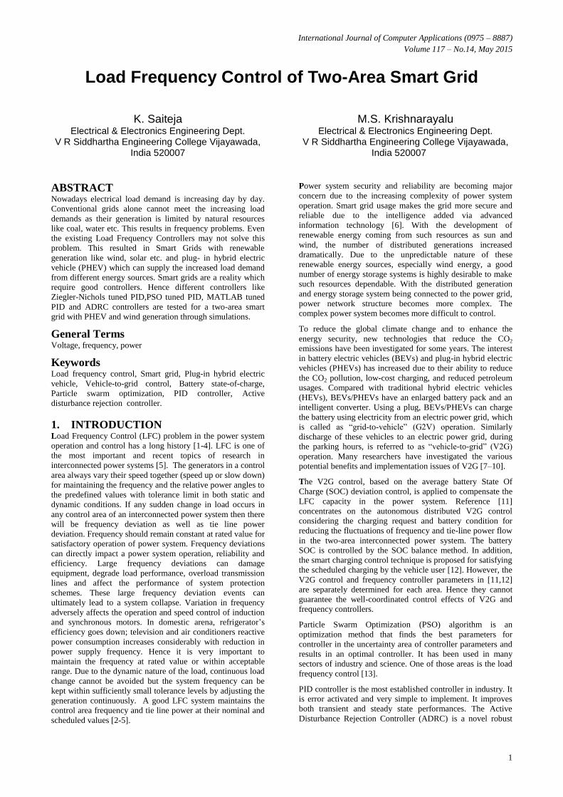
Fig. 2b Subsystem of V2G Model of Area1

Table 1: LFC data in areas 1 and 2

Parameter Area 1 Area 2 Load capacity, PL(MW) 33090

7090

Rated thermal power output, PO

(MW)

24252

5560

Inertia constant, H sec 8.58 9.02

Load damping coefficient,

D (p.u.MW/p,u.Hz)

2 2

Turbine time constant, Tt (sec) 0.25

0.25

Governor time constant, Tg (sec)

0.2 0.2

Re-heat time constant, Trh (sec)

9 9

Governor speed regulation, R (p.u.)

0.05 0.05

Synchronizing coefficient, T

(p.u./rad)

14 14

Load change, (p.u.)

0.2 0.1

Random Generation Range (p.u.) -1.1 ~ 2 -1.1 ~ 2

Random Load Range (p.u.) -0.9~ 0.8 -0.9~ 0.8

Table 2: V2G control data in areas 1 and 2

Parameter Area 1 Area 2 Maximum V2G Power, Pmax (kw)

5 5

Maximum V2G Gain, Kmax

(kw/Hz)

200 200

Design parameter: n

2 2

SOCmin(%) 10 10

SOClow(%) 20 20

SOChigh(%) 80 80

SOCmax(%) 90 90

Initial SOC(%),Target SOC(%) 20, 90 50, 50

Delay time, TPHEV(sec) 1 1

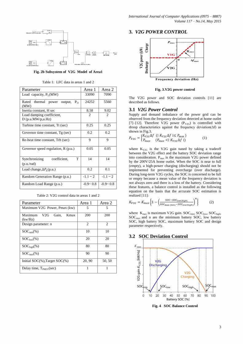
3. V2G POWER CONTROL

Fig. 3.V2G power control

The V2G power and SOC deviation controls [11] are

described as follows.

3.1 V2G Power Control Supply and demand imbalance of the power grid can be

observed from the frequency deviation detected at home outlet

[7]–[12]. Therefore V2G power (PV2G) is controlled with

droop characteristics against the frequency deviation(∆f) as

shown in Fig.3.

(1)

where KV2G is the V2G gain tuned by taking a tradeoff

between the V2G effect and the battery SOC deviation range

into consideration. Pmax is the maximum V2G power defined

by the 200V/25A home outlet. When the SOC is near to full

(empty), a high-power charging (discharging) should not be

implemented for preventing overcharge (over discharge).

During long-term V2G cycles, the SOC is concerned to be full

or empty because a mean value of the frequency deviation is

not always zero and there is a loss of the battery. Considering

these features, a balance control is installed as the following

equation on the basis that the accurate SOC estimation is

realized [11]:

(2)

where Kmax is maximum V2G gain. SOCmin, SOClow, SOChigh,

SOCmax and n are the minimum battery SOC, low battery

SOC, high battery SOC, maximum battery SOC and design

parameter respectively.

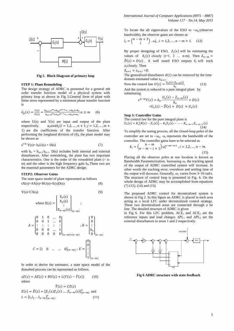
3.2 SOC Deviation Control

Fig. 4 SOC Balance Control


Volume 117 – No.14, May 2015

4

The SOC can be controlled by the SOC balance control as

shown in Fig. 4. Based on (1) and (2), PV2G can be controlled

by tuning the gain KV2G against the frequency deviation.KV2G

can be adjusted by the SOC deviation control within the

specified SOC range. Here, the initial SOC and target SOC in

area 1 are set at 20% and 90%, respectively. Also, in area 2,

the initial SOC and target SOC are set at 50% and 50%,

respectively.

4. CONTROLLERS PID and ADRC controllers are employed as secondary

controllers for the LFC problem. PID controller is tuned by a

number of methods as given below.

4.1 PID Controller Tuning The basic structure of a PID controller is

Gc(s) = KP+ KI/s + KDs (3)

where KP, KI and KD are proportional, integral and derivative

gain constants. Proportional control results in decrease of rise

time but also results in oscillatory performance. Derivative

control reduces the oscillations by providing proper damping

which results in improved transient performance and stability.

Integral control reduces the steady state error to zero.

Theoretically KP, KI and KD are to be selected from infinite

combinations. Proper selection KP, KI and KD is the tuning of

PID controller.

4.1.1Ziegler-Nichols (Z-N) Method In 1942 Ziegler and Nichols, who were engineers for a major

control hardware company in the United States (Taylor

Instruments Co), proposed tuning rules for the ”Optimum

settings for automatic controllers”. Based on their experience

with transients for many types of processes they developed a

method for tuning of closed-loop response. The principal

control effects found in PID-controller were examined and

practical names and units proposed for each effect. They

suggested that ultimate controller gain KU, and ultimate period

PU, were to be obtained from a closed-loop test of the actual

process. When the process is in steady state within the normal

level of operating, the integral and the derivative modes of the

PID-controller are removed leaving only the proportional

control. On some controllers, this might require setting the

deviate time to its minimal value and the integrating time to

its maximum value. Disturb the system by adding an

increasing value of proportional gain to the controller, until

the system response with a sustained constant oscillating

output. The corresponding KU is denoted as the ultimate gain,

and the period of oscillation is the ultimate period, PU. The Z-

N tuning rules [20], given in Table 3,are then used to set the

controller parameters for a Proportional (P), a Proportional-

integral (PI) or a Proportional-integral-derivative (PID)

controller. This Z-N method is very simple to implement.

Table 3: Z-N Tuning Method

Type of Controller KP TI TD

Proportional (P) 0.5 * KU ∞ 0

Proportional-integral (PI) 0.45 * KU

0

Proportional-integral-derivative

(PID)

0.6 * KU

KI = KP/TI ; KD = KP*TD

4.1.2 PSO Tuned PID Particle swarm optimization (PSO) is an evolutionary

computation technique developed by Dr. Eberhart and Dr.

Kennedy in 1995, inspired by social behavior of bird flocking

or fish schooling. PSO is a population based optimization

tool. The system is initialized with a population of random

solutions and searches for optima by updating generations. All

the particles have fitness values, which are evaluated by the

fitness function to be optimized, and have velocities, which

direct the flying of the particles. All particles fly through a

multidimensional search space where each particle is

adjusting its position according to its own experience and

neighbor’s experience. Each particle keeps track of its

coordinates in the solution space which are associated with

the best solution (fitness) that has achieved so far by that

particle. This value is called personal best, pbest. Another best

value that is tracked by the PSO is the best value obtained so

far by any particle in the neighborhood of that particle. This

value is called gbest. The basic concept of PSO lies in

accelerating each particle toward its pbest and the gbest

locations, with a random weighted acceleration at each time

step. Detailed algorithm is available in [13].

The objective function, J for PSO is taken as to minimize the

frequency deviations in areas 1 and 2 as:

J=

(4)

Subject to

4.1.3 MATLAB Tuned PID In MATLAB, the transfer function of PID controller is

(s)

/(s+N)} (5)

where N sets the pole location of derivative noise filter.

Default value of N is 100.PID controller tuning can be

achieved in three steps using MATLAB SIMULINK [19]. In

Step 1 select KP that results in a highly oscillatory stable

response with KD = KI = 0. In Step 2 fix the parameter KD, for

KP selected in Step1, to take care of transient performance. In

Step 3 acquire the parameter KI, for KP and KD selected in

Steps 1 and 2, to take care of steady state performance.

Actually this selection converges to a set of values of KP, KI

and KD. This completes the tuning of PID controller.

Following the above tuning methods the resulting parameters

of PID controller are given in Table 4.

Table 4: PID tuning results

Method Area 1 Area 2

KP KI KD KP KI KD

Z-N 3.307 2.755 1.6 3.307 2.755 1.6

PSO 4.932 0.965 2.7636 11 1.4 3.5

MATLAB 9.5 4.956 4.5 13 1.8 5.5

4.2 ADRC Design [17, 18] Here an (n+1)th-order ESO is used to estimate the n states and

disturbance (internal and external) in order to eliminate the

disturbance. The resulting system acts as an nth order

integrator


Volume 117 – No.14, May 2015

5

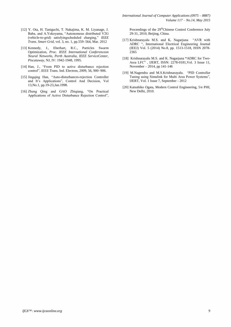
Fig 5. Block Diagram of primary loop

STEP 1: Plant Remodeling

The design strategy of ADRC is presented for a general nth order transfer function model of a physical system with primary loop as shown in Fig 5.General form of plant with finite zeros represented by a minimum phase transfer function is

, (6)

where U(s) and Y(s) are input and output of the plant

respectively.

are the coefficients of the transfer function. After

performing the longhand division of (6), the plant model may

be shown as

sn-m Y(s)= b0U(s) + D(s) (7)

with b0 = bm+1/an+1. D(s) includes both internal and external

disturbances. After remodeling, the plant has two important

characteristics. One is the order of the remodeled plant (= n-

m) and the other is the high frequency gain b0.These two are

the essential parameters for the ADRC design.

STEP2: Observer Gains

The state space model of plant represented as follows

sX(s)=AX(s)+BU(s)+E(s)D(s) (8)

Y(s)=CX(s) (9)

where

In order to derive the estimator, a state space model of the

disturbed process can be represented as follows.

(10)

where

and

. (11)

To locate the all eigenvalues of the ESO to (observer

bandwidth), the observer gains are chosen as

(12)

By proper designing of ESO, will be estimating the

values of closely (i 1, 2 … n-m). Then

. A well tuned ESO outputs will track

closely. Then

= .

The generalized disturbance can be removed by the time domain estimated value

Now the control law

(13)

And the system is reduced to a pure integral plant by substituting

=

Step 3: Controller Gains

The control law for the pure integral plant is (14)

To simplify the tuning process, all the closed-loop poles of the

controller are set to ωc represents the bandwidth of the

controller. The controller gains have to be selected as

(15)

Placing all the observer poles at one location is known as

Bandwidth Parameterization. Increasing ωc the tracking speed

of the output of ADRC controlled system will increase. In

other words the tracking error, overshoot and settling time of

the output will decrease. Generally, ωc varies from 3~10 rad/s.

The structure of control loop is presented in Fig. 6. On the

whole design of ADRC may be accomplished from equations

(7) (12), (14) and (15). The proposed ADRC control for decentralized system is shown in Fig 2. In this figure an ADRC is placed in each area acting as a local LFC under decentralized control strategy. These two decentralized areas are connected through a tie line. The detailed structure of ADRC is given

in Fig 6. For this LFC problem, ACE1 and ACE2 are the

reference inputs and load changes ΔPL1 and ΔPL2 are the

external disturbances in areas 1 and 2 respectively.

Fig 6 ADRC structure with state feedback


Volume 117 – No.14, May 2015

6

The transfer function of primary loop of area 1 is

Here n=5, m=2,n-m=3, = 0.54, =1.544.

Hence b0 = / = 2.85185.

From (7), controller design equation

Y(s) = 2.85185 U(s) + D(s)

The model of ESO is obtained as:

=

+

u+

y =

From (10), (11) and (12) ESO may be written in terms of

observer gains as

=

+

u(t)+

)

=

–

+

u(t)+

The ESO is derived for observer bandwidth = 20 rad/s.

Next controller gains are computed from (15) for controller

bandwidth = 10 rad/s, as

1 = 1000, 2 = 300, 3 = 30.

Similarly for area 2:

The transfer function of primary loop of area 2 is

Here n=5, m=2, n-m=3, = 0.54, =1.624.

Hence b0 = / =0.3325.

Observer Gains: l1=80; l2=2400; l3=32000; l4=160000.

Controller Gains: 1 = 1000; 2 = 300; 3 = 30.

5. SIMULATION RESULTS The SIMULINK model of a two area PHEV based smart grid

with V2G control and wind power generation is shown in Fig.

2. The controllers in areas 1 and 2 are either PID or ADRC

controllers based on the case. Here the system analysis is

carried out as two cases. In case 1 analysis of the system is

performed with step change in load and without wind power

generation. The results are shown in figures 7- 9. In case 2

analysis is executed including random wind power generation

and random load. These results are shown in figures 10-21.

Fig. 7- Frequency Deviations in Area 1

Fig.8-Frequency Deviations in Area 2

Fig.9-Tie-Line Power Deviations


Volume 117 – No.14, May 2015

7

Fig.10- Frequency Deviations in Area 1

Fig.11-Frequency Deviations in Area 2








Volume 117 – No.14, May 2015

8





6. CONCLUSIONS Recent trend in power system operation is smart grid.

Accordingly an attempt is made to provide a better controller

for two-area smart grid power systems. It is studied as two

cases. Incase 1, the behavior of two-area PHEV based smart

grid with V2G Control without wind power generation with

PID controller tuned by Z-N, PSO, MATLAB methods and

ADRC controller is studied. Next as case 2, the behavior of

two-area smart grid with PHEV includingV2G Control and

random wind power generation and random load with PID

and ADRC controllers as mentioned above is analyzed. From

the figures7-21it can be concluded that ADRC controller is

the best with good transient and steady state responses closely

followed by MATLAB tuned PID controller in both cases.

Further this work may be extended to multi-area smart power

grids with robust control as future extension.

7. ACKNOWLEDGMENTS We greatly acknowledge Siddhartha Academy of General and

Technical Education, Vijayawada for providing the facilities

to carry out this research.

8. REFERENCES [1] Hadi Saadat, Power System Analysis, Tata McGraw-Hill,

New Delhi, 2007

[2] Elgerd Ol. Electric energy system theory: an

introduction. 2/e. McGraw Hill, New York:,1983.

[3] Kundur P. Power system stability and control. 5th reprint.

Tata McGraw Hill; New Delhi: 2008.

[4] Kothari DP, Nagrath IJ. Modern power system

analysis.4/e. New Delhi: Tata McGraw Hill; 2011.

[5] Ibraheem, Kumar P, Kothari DP. Recent philosophies of

automatic generation control strategies in power systems.

IEEE Trans Power Syst 2005;20(1):346–57.

[6] U.S. Department of Energy (DOE), “Smart grid system

report,” Jul.2009 [Online]. Available:

http://www.oe.energy.gov/Documentsand-

Media/SGSRMain_090707_lowres.pdf

[7] Y. Ota et al., “Effect of autonomous distributed vehicle-to-

grid (V2G)on power system frequency control,” in Proc.

Int. Conf. Ind. Inf. Syst.(ICIIS), pp. 481–485.

[8] K. Shimizu et al., “Load frequency control in power

system using vehicle-to-grid system considering the

customer convenience of electric vehicles,” in Proc. Int.

Conf. 2010 Power Syst. Technol. (POWERCON),pp. 1–8.

[9] S. W. Hadley and A. Tsvetkova, “Potential impacts of

plug-in hybrid electric vehicles on regional power

generation,” Oak Ridge National Laboratory, Oak Ridge,

TN, ORNL/TM-2007/150, Jan. 2008.

[10] J. R. Pillai and B. Bak-Jensen, “Integration of vehicle-to-

grid in the Western Danish power system,” IEEE Trans.

Sustainable Energy, vol.2, no. 1, pp. 12–19, Jan. 2011.

[11] Sitthidet Vachirasricirikul and Issarachai Nigamroo

“Robust LFC in a Smart Grid with Wind

PowerPenetration by Coordinated V2G Control

andFrequency Controller”, IEEE Trans. Smart Grid, vol.

5, no. 1, pp.371–380, Jan 2014


Volume 117 – No.14, May 2015

9

[12] Y. Ota, H. Taniguchi, T. Nakajima, K. M. Liyanage, J.

Baba, and A.Yokoyama, “Autonomous distributed V2G

(vehicle-to-grid) satisfyingscheduled charging,” IEEE

Trans. Smart Grid, vol. 3, no. 1, pp.559–564, Mar. 2012

[13] Kennedy, J., Eberhart, R.C., Particles Swarm

Optimization, Proc. IEEE International Conferenceon

Neural Networks, Perth Australia, IEEE ServiceCenter,

Piscataway, NJ, IV: 1942-1948, 1995.

[14] Han, J., “From PID to active disturbance rejection

control”, IEEE Trans. Ind. Electron, 2009, 56, 900–906.

[15] Jingqing Han, “Auto-disturbances-rejection Controller

and It’s Applications”, Control And Decision, Vol

13,No.1, pp.19-23,Jan.1998.

[16] Zheng Qing and GAO Zhiqiang, “On Practical

Applications of Active Disturbance Rejection Control”,

Proceedings of the 29thChinese Control Conference July

29-31, 2010, Beijing, China.

[17] Krishnarayalu M.S. and K. Nagarjuna “AVR with

ADRC “, International Electrical Engineering Journal

(IEEJ) Vol. 5 (2014) No.8, pp. 1513-1518, ISSN 2078-

2365

[18] Krishnarayalu M.S. and K. Nagarjuna “ADRC for Two-

Area LFC” , IJERT, ISSN: 2278-0181,Vol. 3 Issue 11,

November – 2014, pp 141-146

[19] M.Nagendra and M.S.Krishnarayalu. “PID Controller

Tuning using Simulink for Multi Area Power Systems”,

IJERT, Vol. 1 Issue 7, September - 2012

[20] Katsuhiko Ogata, Modern Control Engineering, 5/e PHI,

New Delhi, 2010.

IJCATM : www.ijcaonline.org